influence of topographic complexity on solar insolation ... · influence of topographic...
TRANSCRIPT
Ecological Modelling 183 (2005) 157–172
Influence of topographic complexity on solar insolation estimatesfor the Colorado River, Grand Canyon, AZ
Michael D. Yarda,∗, Glenn E. Bennetta, Steve N. Mietza, Lewis G. Coggins Jr.a,Lawrence E. Stevensb, Susan Hueftlea, Dean W. Blinnc
a Grand Canyon Monitoring and Research Center, U.S. Geological Survey, Flagstaff, AZ 86001-1600, USAb Grand Canyon Wildlands Council, Flagstaff, AZ 86001-5467, USA
c Department of Biological Sciences, Northern Arizona University, Flagstaff, AZ 86011-5640, USA
Received 22 July 2003; received in revised form 4 May 2004; accepted 12 July 2004
Abstract
Rugged topography along the Colorado River in Glen and Grand Canyons, exemplifies features common to canyon-boundstreams and rivers of the arid southwest. Physical relief influences regulated river systems, especially those that are altered, andhave become partially reliant on aquatic primary production. We measured and modeled instantaneous solar flux in a topograph-ically complex environment to determine where differences in daily, seasonal and annual solar insolation occurred in this riversystem. At a system-wide scale, topographic complexity generates a spatial and temporal mosaic of varying solar insolation.This solar variation is a predictable consequence of channel orientation, geomorphology, elevation angles and viewshed. Mod-
synthetic
phicwinter.
ariation,itessted fortive stepfor other
eled estimates for clear conditions corresponded closely with observed measurements for both instantaneous photophoton flux density (PPFD:�mol m−2 s−1) and daily insolation levels (relative error 2.3%, CI±0.45, S.D. 0.3,n = 29,813).Mean annual daily insolation levels system-wide were estimated to be 36 mol m−2 d−1 (17.5 S.D.), and seasonally varied onaverage from 13.4–57.4 mol m−2 d−1, for winter and summer, respectively. In comparison to identical areas lacking topograeffect (idealized plane), mean daily insolation levels were reduced by 22% during summer, and as much as 53% duringDepending on outlying topography, canyon bound regions having east–west (EW) orientations had higher seasonal vaveraging from 8.1 to 61.4 mol m−2 d−1, for winter and summer, respectively. For EW orientations, 70% of mid-channel swere obscured from direct incidence during part of the year; and of these sites, average diffuse light conditions persi19.3% of the year (70.5 days), and extended upwards to 194 days. This predictive model has provided an initial quantitato estimate and determine the importance of autotrophic production for this ecosystem, as well as a broader applicationcanyon systems.© 2004 Published by Elsevier B.V.
Keywords:Solar incidence; PPFD; Topographic relief; GIS; Aquatic
∗ Corresponding author. Tel.: +1 928 779 1856.E-mail address:[email protected] (M.D. Yard).
0304-3800/$ – see front matter © 2004 Published by Elsevier B.V.doi:10.1016/j.ecolmodel.2004.07.027
158 M.D. Yard et al. / Ecological Modelling 183 (2005) 157–172
1. Introduction
Vertical relief interferes with incoming solar in-cidence and can dramatically affect ecosystem en-ergetics, particularly in canyon-bound regions oralong densely vegetated streams (Vanote et al., 1980;Hawkins et al., 1982; Monteith and Unsworth, 1990).Physical obstructions are recognized for having pro-nounced effects on daily, seasonal, and annual so-lar insolation levels (Hill, 1996). Subtle differencesin altitude angles, elevation surface gradients, sky-light, and orientation generate varying levels of spa-tio/temporal complexity (Kumar et al., 1997; Dozierand Frew, 1990). In GIS-modeled environments, solarradiation models have been used effectively to estimateinsolation differences on large-scale geographic sur-faces (mountainous and canyon terrain) (Dozier andOutclat, 1979; Rich et al., 1995). However, studieson topographic effects in river ecosystems are un-common, owing perhaps to methodological constraints(e.g., grid-size limitations, sampling devices) used todetermine photosynthetic photon flux density (PPFD:�mol m−2 s−1).
The Colorado River (CR) in Glen and GrandCanyons is representative of topographically complexriverine environments in the arid southwestern UnitedStates. Because of dam-regulation, some of the bio-logical resources in the CR ecosystem are highly af-fected (Blinn and Cole, 1991; Stevens et al., 1997a,1997b), and considerable evidence suggests that thisr u-t eta al.,1 han-n sem seds gp co-l ers.
ersi ri-z andL es Pow-e lenC re-la that
flows through an extensive geographic region wheresuspended-sediment supplied from tributaries limitssubaqueous PPFD (Shaver et al., 1997). Yet, these light-attenuating effects are subsequent to the influence thattopographic relief has on regulating the quantity of in-coming solar incidence received initially at the watersurface.
We examined the role topographic relief has onregulating daily, seasonal and annual solar insolationreaching the CR water surface. Geomorphic controlfunctions at regional and local scales to influence theincised characteristics of this canyon dominated riverby regulating channel meanders, orientation and topog-raphy (Schmidt, 1990; Gregory et al., 1991; Stevens etal., 1997a; Schmidt et al., 1998). Ecologists have facedsimilar problems in other aquatic systems; yet, beyondgeneral site-specific descriptions empirical efforts areoften quantitatively compromised by limited deploy-ment periods or spatial coverage. A number of pre-dictive solar models are available (Dubayah and Rich,1995; Kumar et al., 1997), although some are incom-plete, costly, complicated, or have considerable datarequirements. Thus, our study had multiple objectives:(1) develop a generalized model for estimating instan-taneous solar flux for large rivers containing topograph-ically complex environments and (2) determine wheredifferences in daily, seasonal and annual solar insola-tion occurred along the CR.
2
ns:G yon,a rc ghts,at unitsd iffer-e eris-te la-t amf
2
geo and
iver is light-limited and partially dependent on aotrophic production (Blinn and Cole, 1991; Shaverl., 1997; Stevens et al., 1997a, 1997b; Blinn et998; Benenati et al., 2000; Walters et al., 2000; Son et al., 2001). This condition is unusual, becauost large rivers are primarily an allochthonous ba
ystem (Haden et al., 1999); therefore, understandinhysical factors limiting PPFD has considerable e
ogical significance for this and other regulated rivThe CR is one of the most regulated large riv
n the US that flows 475 km through northern Aona between two large reservoirs, Lake Powellake Mead (Stevens et al., 1997a, 1997b). Becaususpended-sediment is now sequestered in Lakell reservoir, hypolimnetic flows released from Ganyon Dam (GCD) are highly transparent. Dam
eases typically fluctuate from 142 to 708 m3 s−1 ondiurnal schedule. This is a very turbulent river
. Methods
Study area includes four major canyon sectiolen Canyon, Marble Canyon, Central Grand Cannd Western Grand Canyon (Fig. 1). These largeanyon sections have varying channel widths, heind orientations (Stevens et al., 1997a, 1997b). Con-
ained within these major canyon sections are subescribed as geomorphic reaches, each having dnt topographic, stratigraphic and erosive charact
ics (Howard and Dolan, 1981; Schmidt, 1990; Stevenst al., 1997a) (Table 1). Locations are described in re
ion to distance in river kilometers (Rkm) downstrerom GCD (0.0 Rkm).
.1. Solar and ground incidence
Solar flux is distributed over a broad ranf wavelengths and peaks within the visible b
M.D. Yard et al. / Ecological Modelling 183 (2005) 157–172 159
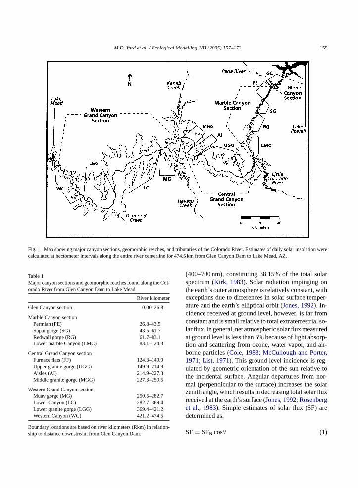
Fig. 1. Map showing major canyon sections, geomorphic reaches, and tributaries of the Colorado River. Estimates of daily solar insolation werecalculated at hectometer intervals along the entire river centerline for 474.5 km from Glen Canyon Dam to Lake Mead, AZ.
Table 1Major canyon sections and geomorphic reaches found along the Col-orado River from Glen Canyon Dam to Lake Mead
River kilometer
Glen Canyon section 0.00–26.8
Marble Canyon sectionPermian (PE) 26.8–43.5Supai gorge (SG) 43.5–61.7Redwall gorge (RG) 61.7–83.1Lower marble Canyon (LMC) 83.1–124.3
Central Grand Canyon sectionFurnace flats (FF) 124.3–149.9Upper granite gorge (UGG) 149.9–214.9Aisles (AI) 214.9–227.3Middle granite gorge (MGG) 227.3–250.5
Western Grand Canyon sectionMuav gorge (MG) 250.5–282.7Lower Canyon (LC) 282.7–369.4Lower granite gorge (LGG) 369.4–421.2Western Canyon (WC) 421.2–474.5
Boundary locations are based on river kilometers (Rkm) in relation-ship to distance downstream from Glen Canyon Dam.
(400–700 nm), constituting 38.15% of the total solarspectrum (Kirk, 1983). Solar radiation impinging onthe earth’s outer atmosphere is relatively constant, withexceptions due to differences in solar surface temper-ature and the earth’s elliptical orbit (Jones, 1992). In-cidence received at ground level, however, is far fromconstant and is small relative to total extraterrestrial so-lar flux. In general, net atmospheric solar flux measuredat ground level is less than 5% because of light absorp-tion and scattering from ozone, water vapor, and air-borne particles (Cole, 1983; McCullough and Porter,1971; List, 1971). This ground level incidence is reg-ulated by geometric orientation of the sun relative tothe incidental surface. Angular departures from nor-mal (perpendicular to the surface) increases the solarzenith angle, which results in decreasing total solar fluxreceived at the earth’s surface (Jones, 1992; Rosenberget al., 1983). Simple estimates of solar flux (SF) aredetermined as:
SF= SFN cosθ (1)
160 M.D. Yard et al. / Ecological Modelling 183 (2005) 157–172
where SFN is solar flux normal to surface, andθ iszenith angle, representing the angle between the di-rect beam and normal; therefore asθ increases, SF de-creases.
In addition toθ, the depth of the overlying air-massinfluences the degree of atmospheric absorption, reflec-tion, and refraction, such that SF decreases exponen-tially as a function of optical depth (Page and Sharples,1988; Kasten and Young, 1989). Beer’s law describesthis relationship as:
SF= SF0e(−Kz) (2)
where SF0 is initial solar flux,K is coefficient of at-mospheric light-attenuation, and SF is resulting in-tensity after a known optical depth (z) through agiven air-mass (Stine and Harrigan, 1985; Kasten andYoung, 1989). Yet, accounting for multiple-light at-tenuating factors requires considerable knowledge ofatmospheric conditions (e.g., climate, transmissivity,atmospheric pressure, and cloud cover), and for allpracticality atmospheric data are not sufficiently robustor available for most localities (List, 1971). This oftenprecludes using more conventional methods for esti-mating SF. We used an alternative approach wherebywe substituted SFN for a parameter called normal-ized ground incidence (GIN). This parameter representsmaximum SF received at ground surface followingatmospheric light-attenuation ifθ were normal (θ =0◦) and assumes that factors contributing to light-a mp-t ricc ee rrorv ev-e
r sur-f fora esf d fort -t uetS
2
t the
mathematical coordinate system used to estimate solarangles requires knowing the spatio/temporal relation-ships specific to a site location. Solar coordinates arebased on solar time (ST), thus differences among lo-cal standard time (LST) and ST must be considered.Converting LST to ST requires two adjustments. Thefirst accounts for differences in longitude among stan-dard meridianLST and observation locationLOB. Weused a correction of±4 min (i.e., positive east and neg-ative west) for every degree longitude (Rapp, 1981).Secondly, seasonal differences among LST and ST(±16 min) are related to the earth’s elliptical orbit andinclination relative to solar orbital plane. The equationof time (E) accounts for the earth-sun geometric rela-tionship, and is calculated from:
E = 9.87 sin
[2(360(Jday− 81))
365
]
− 7.53 cos
[360(Jday− 81)
365
]
− 1.5 sin
[360(Jday− 81)
365
](3)
where daily differences in ST relative to LST are cor-rected by Julian date (Jday) (Cousins, 1969). By com-bining temporal adjustments, ST is calculated from
ST = LST + 3.989(LST − LOB) + E (4)
where LST is local standard time,LST is standardmo
lartv ,1
δ
T uref -i rrectf udea r be-t atelye :
θ
ttenuation remain constant. Validity of this assuion is contingent on the variability of local atmospheonditions. Therefore, constancy of GIN requires sommpirical grounding to determine whether the earies systematically (spatio/temporal) or within lls acceptable to researchers.
To address this, we used data measured at wateace (LiCor, Inc., LI-190SA) representing PPFD
wide range ofθ angles collected at multiple sitor different years, seasons, and times. We solvehe best estimate of GIN using a non-linear optimizaion program and applying a minimization techniqhat reduced the sum of squared residuals (Frontlinesystems, Inc. 1999).
.2. Solar coordinates and zenith angle
The above relationships indicate thatθ is impor-ant for estimating daily solar insolation because
eridian,LOB is observed meridian, andE is equationf time.
Solar declination (δ) represents the earth’s anguilt to the sun, which shifts seasonally±23◦26′ betweenernal and autumnal equinoxes (Duffie and Beckman980). Declination is calculated using:
= 23.439 sin
[360
(283+ Jday
365
)]. (5)
he hour angle (ω) represents the angle of departrom solar noon (0◦), which varies±15 h−1, (i.e., postive east and negative west) and is used to coor temporal deviations due to differences in longitmong sites, and seasonal differences that occu
ween LST and ST. Since ST is needed to accurstimate solar coordinates,ω allowsθ to be estimated
= cos−1(sinδ sinϕ + cosδ cosϕ cosω), (6)
M.D. Yard et al. / Ecological Modelling 183 (2005) 157–172 161
where δ is declination angle,ϕ is observed latitudefor the observed site, andω is hour angle. For a morerigorous explanation of these predictive relationshipsrefer toForsythe et al. (1995), Mueller (1977), Rapp(1981), Stine and Harrigan (1985), andCampbell andNorman (1998).
2.3. Estimating photosynthetic photon flux density
Following effects from atmospheric light-attenuation, normal ground incidence GIN is par-titioned into sub-components, representing directbeam GIDB = GIN (x) and diffuse incidence GIDI= GIN (1 − x). The variable “x” is equivalent to aproportion of direct solar beam in relation to total solarincidence. The proportion of ground incidence (x =GIDB/GIN) received directly from direct solar beam isconsidered to be approximately 75% of the total solarflux (Monteith and Unsworth, 1990). Even thoughGIDB is highly directional relative to GIDI (downwardangle across the skylight) total ground incidence (GI)can be estimated
GI = cosθ(GIDB + GIDI). (7)
The temporal reference used for sunrise and sunset isa geometric definition based on the solar disc centerperpendicular to normal (θ = 90◦). Yet, unlike directsolar beam, atmospheric scattering of diffuse incidenceis measurable prior to sunrise and sunset time. There-f T)w T oc-ca omg termi un-s aren dif-f efineo6 ced cteda
ctor( win-t , ana ilyd ssed
by:
sd= 1 + cos
[((Jday− 3)
360
365.2422
)0.0344
](8)
where, 360 represents the earth’s solar rotation,365.2442 is number of days for an annual rotation, and±3.44% is a distance offset. This results in a linear cor-rection (astronomical units) to GIN between 1.0344%on 3 January, to 0.9674% by 5 July (Thekaekara, 1977).
Although solar coordinates for the geometric centerof sunrise and sunset can be derived, topographic reliefis important when obstructive features vary in eleva-tion along the solar ephemeris, as well as its influenceon the proportion of visible skylight, here after referredto as viewshed (VP). For this reason we estimated: (1)solar times for direct-rise and direct-set of the GIDBfor each Jday, (2)VP and (3) canyon orientation. Topo-graphic elevation angles were estimated using a geo-graphical information system (GIS) hillshade function(ESRI, Inc., 2002) on a digital elevation model (DEM,10 m cell size) for sites located on the CR centerlineat 100 m intervals from Glen Canyon Dam to PierceFerry (Mietz and Gushue, 2002).
Diffuse incidence increases at angles adjacent todirect angular beam, and conversely decreases withgreater zenith angles. Any decrease in viewshed re-duces the quantity of diffuse incidence, even thoughthe overall proportion may be small (≤25%) in rela-tion to the direct solar beam (Monteith and Unsworth,1 sst lg
G
2
adef s,r or ag voidc lti-t -s phicfm .a ver a
ore, the reference angle defined as civil twilight (Cas used to regulate direct beam exposure. The Curs when the center of the sun is 6◦ below horizonnd has approximately a 24 min time difference freometric sunrise and sunset time. The temporal
nitiating GIDB is based on geometric sunrise and set (θDB = θ) (temporal differences due to refractionot considered). However, to account for temporal
erences among diffuse and direct incidence, we dnset and end time for GIDI based on CT (θDI = θ −◦). Our relationship for estimating ground incidenoes not differentiate between proportions of reflelbedo to reflected skylight.
At northern latitudes, the shortest radius veearth center to sun center) distance occurs duringer periods. Because of earth’s asymmetric orbitdjustment to GIN must be made to account for daifferences in solar distance (sd). This is expre
990). Clearly, GIDI is not evenly distributed acroheVP, although we assume thatVP ≈ GIDI. The totaround incidence is estimated by:
I = [(cosθDB × GIDB) + (cosθDI × GIDI × VP)]
(9)
.4. Topographic complexity
We used an arc-info routine referred to as hillshunction (ESRI, Inc., 2002) to generate binary gridepresenting areas of shadow and illumination fiven set of azimuths and altitude angles. To aonfusion, we distinguish between two types of aude angles. Elevation angles (ΨE) refer to angles meaured from a horizontal surface relative to a topograeature, whereas illumination angles (Ψ I ) refer to theaximal angle between the topography and skylineΨ Ingles were sequentially searched incrementally o
162 M.D. Yard et al. / Ecological Modelling 183 (2005) 157–172
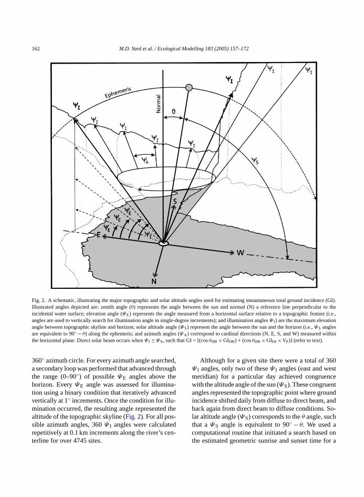
Fig. 2. A schematic, illustrating the major topographic and solar altitude angles used for estimating instantaneous total ground incidence (GI).Illustrated angles depicted are: zenith angle (θ) represents the angle between the sun and normal (N) a reference line perpendicular to theincidental water surface; elevation angle (ΨE) represents the angle measured from a horizontal surface relative to a topographic feature (i.e.,angles are used to vertically search for illumination angle in single-degree increments); and illumination anglesΨ I ) are the maximum elevationangle between topographic skyline and horizon; solar altitude angle (ΨS) represent the angle between the sun and the horizon (i.e.,ΨS anglesare equivalent to 90◦ − θ) along the ephemeris; and azimuth angles (ΨA) correspond to cardinal directions (N, E, S, and W) measured withinthe horizontal plane. Direct solar beam occurs whenΨ I ≤ΨS, such that GI = [(cosθDB × GIDB) + (cosθDB × GIDI ×VP)] (refer to text).
360◦ azimuth circle. For every azimuth angle searched,a secondary loop was performed that advanced throughthe range (0–90◦) of possibleΨE angles above thehorizon. EveryΨE angle was assessed for illumina-tion using a binary condition that iteratively advancedvertically at 1◦ increments. Once the condition for illu-mination occurred, the resulting angle represented thealtitude of the topographic skyline (Fig. 2). For all pos-sible azimuth angles, 360Ψ I angles were calculatedrepetitively at 0.1 km increments along the river’s cen-terline for over 4745 sites.
Although for a given site there were a total of 360Ψ I angles, only two of theseΨ I angles (east and westmeridian) for a particular day achieved congruencewith the altitude angle of the sun (ΨS). These congruentangles represented the topographic point where groundincidence shifted daily from diffuse to direct beam, andback again from direct beam to diffuse conditions. So-lar altitude angle (ΨS) corresponds to theθ angle, suchthat aΨS angle is equivalent to 90◦ − θ. We used acomputational routine that initiated a search based onthe estimated geometric sunrise and sunset time for a
M.D. Yard et al. / Ecological Modelling 183 (2005) 157–172 163
particular day. For every day, topographic direct-riseand direct-set times were determined by sequentiallycomparing allΨ I (direct rise and set) to knownΨS an-gles found within the solar ephemeris. This routine wasperformed in 1 min time increments until the congru-ent conditionΨ I ≥ΨS occurred. ResultingΨ I anglerepresented the angular location and solar time whentopography no longer obstructed direct solar beam. Allestimated times for direct solar beam were site depen-dent and varied daily due to changes in observed lati-tude, declination, and topographic relief; and based onthis temporal condition the term (cosθDB · GIDB) waseither used or excluded from Eq.(9).
Proportional area of the viewshed (VP) was deter-mined using analytical geometry (Anton, 1984), wherefor each azimuth angle (i), arc- or sky angle (αi) wasdetermined from the correspondingΨ Ii angle to nor-mal (αi = 90◦ −Ψ Ii), such that the total proportion ofvisible sky was described by:
VP =
360∑i=1αi/90
360
. (10)
Only one of four possible channel orientations is as-signed to each site, these cardinal directions included:north–south (NS), northwest–southeast (NW–SE),east–west (EW), and northeast–southwest (NE–SW).Channel orientation was determined for each site us-i glesa n thelp tingc
-j at-te go d fort de-r tan-t times overo lop am ano us-i d in-
stantaneous PPFD estimates at smaller time increments(Yard, 2003). Although, our approach lacks an elegantintegration of insolation, it allows us to dynamicallycontrol for other environmental variables operating atsmaller time increments.
2.5. Statistical analysis
Main effects ANOVA (Type VI unique) was used totest for seasonal mean differences and interactions ofdaily solar insolation among canyon sections, geomor-phic reaches, and channel orientation (Sokal and Rohlf,1995). Multiple comparison procedures (Single-factorANOVA and Tukey unequal NHSD) were used as posthoc tests to determine group mean differences. Simplelinear regressions and bootstrap techniques were usedto compare differences among observed and predictedestimates of GIN (Neter et al., 1996). We determinedrelative error in our modeled estimates from atmo-spheric influence under clear or cloudy conditions. Us-ing a bootstrap technique, observed data for a rangeof varying atmospheric conditions were analyzed todetermine relative error (RE = (E−O)/O) representingthe estimated error (E) relative to an observed mea-surement (O). Data used for this analysis were inde-pendent from data previously used for estimating pa-rameter GIN. Data were segregated, representing eitherclear skies or cloudy conditions. For each resample,500 random samples were selected from empirical datafor clear skies (n = 29,813) cloudy skies (n = 25,051),a si ot-s used( .,2
3
( dc oft atau om1 esf Ivd
ng a routine that searched all possible azimuth annd selected a discrete cardinal direction based o
owestΨ I angles encountered in theVP. Ortho-rectifiedhotos were used to validate method for estimahannel orientation.
Empirical data for PPFD (�mol m−2 s−1) were adusted to normal by accounting for differencesributed toθ (Eq. (6)) and solar distance (Eq.(8)). Westimated the parameter GIN (Eq. (9)) by regressinbserved against estimated incidence and solve
he best fit. Daily solar insolation estimates wereived using a numerical solution that estimated insaneous PPFD through summation over discreteteps (1 min intervals). We chose this approachther methods because our purpose was to deveethod for estimating aquatic primary production inptically and hydrologically variable environment
ng a discrete-state modeling approach that require
nd intermittent clouds (n = 9275). Median RE wateratively sampled with replacement for 10,000 botrap samples. Multiple statistical packages wereStatistica Statsoft, Inc., 1997; Resampling Stats, Inc001).
. Results
Our estimated GIN was 2326�mol m−2 s−1
r2 = 0.94, n= 4312, S.E.± 36.3) that representelear-sunny daytime conditions characteristichis large geographical region. Observed dsed for estimating this parameter varied fr321–2063�mol m−2 s−1, and included zenith angl
rom 12.79◦–49.79◦. Solar distance adjustment to GNaried linearly 2326± 80�mol m−2 s−1 over a 182.5ays period (Eq.(8)).
164 M.D. Yard et al. / Ecological Modelling 183 (2005) 157–172
3.1. Relative error in estimation of instantaneousincidence
Data were collected over a range of field con-ditions, and different years (1992–2001), seasons,and times and sites. Instantaneous PPFD averaged1052�mol m−2 s−1 and varied between 0.15 and2100�mol m−2 s−1. Although a strong correlation(p< 0.001,r2 = 0.987,n= 58,060) existed among ob-served and estimated data, variation in solar in-cidence increased during periods of continuous orintermittent cloud cover. Our median RE for ob-served incidence under clear skies for all seasonswas 2.3%, with a 95% bootstrap confidence inter-val (CI95%) of 1.85–2.75%; whereas, under cloudyconditions median RE was 100%, with a CI95%
of 92.5–107.5%. RE was most pronounced duringlate-July through September monsoons, and winter(December–March) when cloud cover was greatest.However, an inverse response occurred during inter-mittent cloud cover, which had an estimated inci-dence less than observed (−2%), and had a CI95% of−1.8 to −2.2%. This heightened response was per-haps due to enhanced atmospheric scattering (Kirk,1983).
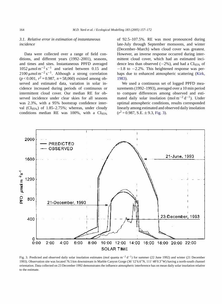
We used a continuous set of logged PPFD mea-surements (1992–1993), averaged over a 10 min periodto compare differences among observed and esti-mated daily solar insolation (mol m−2 d−1). Underoptimal atmospheric conditions, results correspondedlinearly among estimated and observed daily insolation(r2 = 0.987, S.E.± 9.3,Fig. 3).
F s (mol ber1 arble C elot
ig. 3. Predicted and observed daily solar insolation estimate993). Observation site was located 76.5 km downstream in M
rientation. Data collected on 23 December 1992 demonstrates the ino the estimate.
quanta m−2 d−1) for summer (22 June 1992) and winter (21 Decemanyon Gorge (36◦12′6.6′′N, 111◦48′0.3′′W) having a north-south chann
fluence atmospheric interference has on mean daily solar insolation relative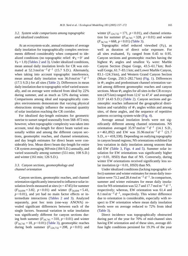
M.D. Yard et al. / Ecological Modelling 183 (2005) 157–172 165
3.2. System wide comparisons among topographicand idealized conditions
At an ecosystem-scale, annual estimates of averagedaily insolation for topographically complex environ-ments differed considerably when compared to ide-alized conditions (no topographic relief:ΨE = 0◦ andVP = 1.0) (Tables 2 and 3). Under idealized conditions,mean annual daily insolation levels for CR was esti-mated at 52.3 mol m−2 d−1 (15.7 S.D.). Alternately,when taking into account topographic interference,mean annual daily insolation was 36.0 mol m−2 d−1
(17.5 S.D.) for all sites (Table 2). Differences in meandaily insolation due to topographic relief varied season-ally, and on average were reduced from ideal by 22%during summer, and as much as 53% during winter.Comparisons among ideal and topographically com-plex environments demonstrate that varying physicalobstructions strongly influence the seasonal quantityof solar insolation reaching the CR corridor.
For idealized day-length estimates for geometricsunrise to sunset ranged seasonally from 568–872 min;however, when topographic complexity was taken intoaccount, total day-length for direct beam varied sea-sonally within and among the different canyon sec-tions, geomorphic reaches, and channel orientations,and day length estimates for direct beam were con-siderably less. Mean direct beam day-length for entireCR system averaging 369 min (184 S.D.) annually, andvaried seasonally among summer (551 min; 108 S.D.)a
3c
nnelo r in-s r(p in-ts re-v thes tionw ur-i r( sd
winter (F124,732= 171,p< 0.01), and channel orienta-tion for summer (F34,741= 328, p< 0.01) and winter(F34,741= 668,p< 0.01) (Table 3).
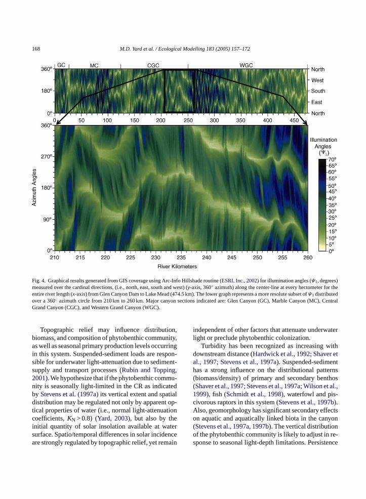
Topographic relief reduced viewshed (VP), aswell as duration of direct solar exposure. Forall sites evaluated,VP ranged from 0.45 to 0.95.Canyon sections and geomorphic reaches having thehighest Ψ I angles and smallestVP were: MarbleCanyon Section (Supai Gorge, 43.5–61.7 km; Red-wall Gorge, 61.7–83.1 km; and Lower Marble Canyon,83.1–124.3 km), and Western Grand Canyon Section(Muav Gorge, 250.5–282.7 km) (Fig. 1). Differencesin Ψ I angles and predominant channel orientation var-ied among different geomorphic reaches and canyonsections. MeanΨ I angles for all sites in the CR ecosys-tem (475 km) ranged from 12.6◦ to 47.4◦ and averaged33.9◦ (4.43 S.D.) (Table 2). Canyon sections and ge-omorphic reaches influenced the geographical distri-bution and variability ofΨ I angles within and amongsites, of these angles, and the sequence of repetitivepatterns occurring system-wide (Fig. 4).
Average annual insolation levels were not sig-nificantly different among channel orientations. NSorientation averaged 35.97 mol m−2 d−1 (14.1 S.D.,n= 461,892) and EW was 35.96 mol m−2 d−1 (21.7S.D.,n= 418,338). Depending on outlying topographyin canyon bound regions; NS orientations exhibited farless variation in daily insolation among seasons thandid EW (Table 3, Figs. 4 and 5). Summer solar in-solation for EW orientations was significantly higher( ingw so-l
ef-f nso-l ,s ola-tr and8 ced re-s tionl deal(
tedd itesh dif-f ear
nd winter (161 min; 126 S.D.).
.3. Canyon sections, geomorphology andhannel orientation
Canyon sections, geomorphic reaches, and charientation significantly interacted to influence solaolation levels measured at sites (n= 4745) for summeF54,694= 3.82, p< 0.01) and winter (F54,694= 5.41,< 0.01), and yet had no main factor effects or
ermediate interactions (Tables 2 and 3). Analyzedeparately, post hoc tests (one-way ANOVA)ealed significant differences between each ofingle factors. Seasonal variation in solar insolaas significantly different for canyon sections d
ng both summer (F34,741= 310,p< 0.01) and winteF34,741= 18,p< 0.01) (Table 3), geomorphic reacheuring both summer (F124,732= 208, p< 0.01) and
p< 0.01, HSD) than that of NS. Conversely, durinter EW orientations received significantly less
ar insolation (p< 0.01, HSD) than NS.Under idealized conditions (lacking topographic
ect) summer and winter estimates for mean daily iation were 73.2 and 28.4 mol m−2 d−1. In comparisonummer and winter estimates for mean daily insion for NS orientation was 52.7 and 17.7 mol m−2 d−1,espectively; whereas, EW orientation was 61.4.1 mol m−2 d−1, respectively. This winter differenue to orientation is considerable, especially withpect to EW orientation where mean daily insolaevels were on average reduced to 72% from iTable 3).
Direct incidence was topographically obstrucuring part of the year for 70% of mid-channel saving EW orientation and of these sites, average
use light conditions persisted for 19.3% of the y
166M.D.Yardetal./E
colog
icalM
odellin
g183(2005)157–172
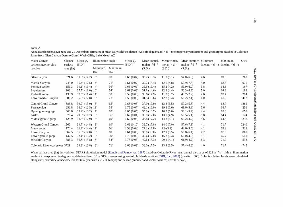
Table 2Annual and seasonal (21 June and 21 December) estimates of mean daily solar insolation levels (mol quanta m−2 d−1) for major canyon sections and geomorphic reaches in ColoradoRiver from Glen Canyon Dam to Grand Wash Cliffs, Lake Mead, AZ
Major Canyonsections geomorphicreaches
Channelsurfacearea (ha)
MeanψE
(S.D.)Illumination angle MeanVp
(S.D.)Mean annual,mol m−2 d−1
(S.D.)
Mean winter,mol m−2 d−1
(S.D.)
Mean summer,mol m−2 d−1
(S.D.)
Minimum(mol m−2 d−1)
Maximum(mol m−2 d−1)
Sites
Minimum(ψI )
Maximum(ψI )
Glen Canyon 321.6 31.3◦ (14.2) 3◦ 70◦ 0.65 (0.07) 35.2 (18.3) 11.7 (6.1) 57.0 (6.8) 4.6 69.0 268
Marble Canyon 743.0 35.4◦ (12.5) 4◦ 71◦ 0.61 (0.07) 32.2 (15.4) 12.5 (4.8) 50.9 (7.3) 4.0 68.3 975Permian section 156.3 30.1◦ (13.4) 4◦ 56◦ 0.68 (0.06) 36.6 (15.4) 15.2 (4.2) 55.9 (6.0) 5.8 68.3 167Supai gorge 103.1 37.7◦ (11.0) 10◦ 54◦ 0.61 (0.03) 31.8 (14.6) 12.3 (4.4) 50.3 (6.3) 5.0 64.3 182Redwall gorge 130.9 37.5◦ (11.4) 11◦ 53◦ 0.59 (0.06) 30.6 (14.9) 11.2 (3.7) 48.7 (7.2) 4.6 62.4 214Lower marble Canyon 386.2 35.5◦ (12.8) 5◦ 71◦ 0.59 (0.06) 31.5 (15.6) 12.2 (5.4) 50.2 (7.1) 4.0 61.9 412
Central Grand Canyon 886.8 34.2◦ (13.0) 6◦ 65◦ 0.68 (0.06) 37.9 (17.9) 13.3 (6.5) 59.2 (5.3) 4.4 68.7 1262Furnace flats 256.8 36.6◦ (12.5) 11◦ 55◦ 0.75 (0.07) 42.1 (16.0) 19.8 (5.6) 61.6 (5.8) 5.6 68.7 256Upper granite gorge 360.8 35.2◦ (13.2) 7◦ 65◦ 0.65 (0.05) 35.9 (18.7) 10.2 (5.6) 58.1 (5.4) 4.4 65.8 650Aisles 76.4 29.3◦ (10.7) 6◦ 55◦ 0.67 (0.01) 38.0 (17.0) 13.7 (4.9) 58.5 (5.1) 5.8 64.4 124Middle granite gorge 125.9 31.5◦ (12.9) 6◦ 60◦ 0.69 (0.03) 38.8 (17.2) 14.2 (5.1) 60.2 (3.2) 5.6 64.8 232
Western Grand Canyon 1562 34.7◦ (14.8) 8◦ 69◦ 0.66 (0.10) 36.7 (17.8) 14.0 (7.0) 57.6 (7.3) 4.1 71.7 2240Muav gorge 170.4 36.7◦ (14.4) 11◦ 66◦ 0.53 (0.03) 27.2 (17.8) 7.0 (3.1) 48.6 (9.5) 4.1 63.2 322Lower Canyon 662.5 36.0◦ (14.8) 8◦ 69◦ 0.64 (0.09) 35.0 (18.0) 12.1 (6.5) 56.8 (6.4) 4.2 67.0 867Lower granite gorge 142.5 32.4◦ (15.2) 8◦ 59◦ 0.70 (0.05) 39.4 (17.0) 15.2 (6.4) 60.0 (4.0) 5.1 65.7 518Western Canyon 586.3 30.8◦ (13.8) 8◦ 54◦ 0.75 (0.05) 42.6 (15.3) 20.1 (4.1) 61.9 (4.2) 6.3 71.7 533
Colorado River ecosystem 3721 33.9◦ (13.8) 3◦ 71◦ 0.66 (0.09) 36.0 (17.5) 13.4 (6.5) 57.4 (6.8) 4.0 71.7 4745
Water surface area (ha) derived from STARS simulation model (Randle and Pemberton, 1987) based on Colorado River mean annual discharge of 323 m−3 s−1. Mean illuminationangles (ψI ) expressed in degrees, and derived from 10 m GIS coverage using arc-info hillshade routine (ESRI, Inc., 2002) (n= site× 360). Solar insolation levels were calculatedalong river centerline at hectometers for total year (n= site× 366 days) and season (summer and winter solstice;n= site× days).
M.D. Yard et al. / Ecological Modelling 183 (2005) 157–172 167
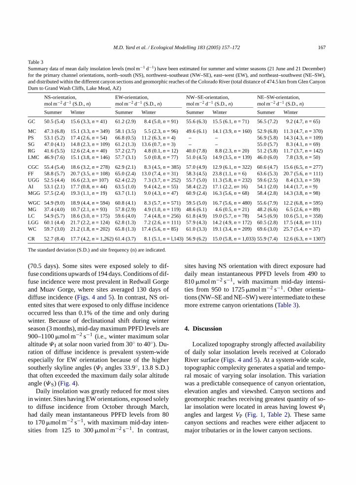
Table 3Summary data of mean daily insolation levels (mol m−1 d−1) have been estimated for summer and winter seasons (21 June and 21 December)for the primary channel orientations, north–south (NS), northwest–southeast (NW–SE), east–west (EW), and northeast–southwest (NE–SW),and distributed within the different canyon sections and geomorphic reaches of the Colorado River (total distance of 474.5 km from Glen CanyonDam to Grand Wash Cliffs, Lake Mead, AZ)
NS-orientation,mol m−2 d−1 (S.D.,n)
EW-orientation,mol m−2 d−1 (S.D.,n)
NW–SE-orientation,mol m−2 d−1 (S.D.,n)
NE–SW-orientation,mol m−2 d−1 (S.D.,n)
Summer Winter Summer Winter Summer Winter Summer Winter
GC 50.5 (5.4) 15.6 (3.3,n = 41) 61.2 (2.9) 8.4 (5.0,n = 91) 55.6 (6.3) 15.5 (6.1,n = 71) 56.5 (7.2) 9.2 (4.7,n = 65)
MC 47.3 (6.8) 15.1 (3.3,n = 349) 58.1 (3.5) 5.5 (2.3,n = 96) 49.6 (6.1) 14.1 (3.9,n = 160) 52.9 (6.8) 11.3 (4.7,n = 370)PS 53.1 (5.2) 17.4 (2.6,n = 54) 66.8 (0.5) 11.2 (6.3,n = 4) – – 56.9 (5.8) 14.3 (4.3,n = 109)SG 47.0 (4.1) 14.8 (2.3,n = 109) 61.2 (1.3) 13.6 (0.7,n = 3) – – 55.0 (5.7) 8.3 (4.1,n = 69)RG 41.6 (5.5) 12.6 (2.4,n = 40) 57.2 (2.7) 4.8 (0.1,n = 12) 40.0 (7.8) 8.8 (2.3,n = 20) 51.2 (5.8) 11.7 (3.7,n = 142)LMC 46.9 (7.6) 15.1 (3.8,n = 146) 57.7 (3.1) 5.0 (0.8,n = 77) 51.0 (4.5) 14.9 (3.5,n = 139) 46.0 (6.0) 7.8 (3.9,n = 50)
CGC 55.4 (5.4) 18.6 (3.2,n = 278) 62.9 (2.1) 8.3 (4.5,n = 385) 57.0 (4.9) 12.9 (6.1,n = 322) 60.6 (4.7) 15.6 (6.5,n = 277)FF 58.8 (5.7) 20.7 (3.5,n = 108) 65.0 (2.4) 13.0 (7.4,n = 31) 58.3 (4.5) 23.8 (1.1,n = 6) 63.6 (5.3) 20.7 (5.6,n = 111)UGG 52.5 (4.4) 16.6 (2.3,n= 107) 62.4 (2.2) 7.3 (3.7,n = 252) 55.7 (5.0) 11.3 (5.8,n = 232) 59.6 (2.5) 8.4 (3.3,n = 59)AI 53.1 (2.1) 17.7 (0.8,n = 44) 63.5 (1.0) 9.4 (4.2,n = 55) 58.4 (2.2) 17.1 (2.2,n= 16) 54.1 (2.0) 14.4 (1.7,n = 9)MGG 57.5 (2.4) 19.3 (1.1,n = 19) 63.7 (1.1) 9.0 (4.3,n = 47) 60.9 (2.4) 16.3 (5.6,n = 68) 58.4 (2.8) 14.3 (3.8,n = 98)
WGC 54.9 (9.0) 18.9 (4.4,n = 594) 60.8 (4.1) 8.3 (5.7,n = 571) 59.5 (5.0) 16.7 (5.6,n = 480) 55.6 (7.9) 12.2 (6.8,n = 595)MG 37.4 (4.0) 10.7 (2.1,n = 93) 57.8 (2.9) 4.9 (1.0,n = 119) 48.6 (6.1) 4.6 (0.5,n = 21) 48.2 (6.6) 6.5 (2.6,n = 89)LC 54.9 (5.7) 18.6 (3.0,n = 175) 59.6 (4.0) 7.4 (4.8,n = 256) 61.8 (4.9) 19.0 (5.7,n = 78) 54.5 (6.9) 10.6 (5.1,n = 358)LGG 60.1 (4.4) 21.7 (2.2,n = 124) 62.8 (1.3) 7.2 (2.6,n = 111) 57.9 (4.3) 14.2 (4.9,n = 172) 60.5 (2.8) 17.5 (4.8,n= 111)WC 59.7 (3.0) 21.2 (1.8,n = 202) 65.8 (1.3) 17.4 (5.6,n = 85) 61.0 (3.3) 19.1 (3.4,n = 209) 69.6 (3.0) 25.7 (5.4,n = 37)
CR 52.7 (8.4) 17.7 (4.2,n = 1,262) 61.4 (3.7) 8.1 (5.1,n = l,143) 56.9 (6.2) 15.0 (5.8,n = 1,033) 55.9 (7.4) 12.6 (6.3,n = 1307)
The standard deviation (S.D.) and site frequency (n) are indicated.
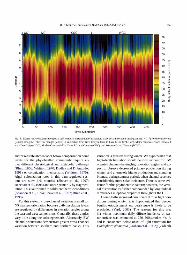
(70.5 days). Some sites were exposed solely to dif-fuse conditions upwards of 194 days. Conditions of dif-fuse incidence were most prevalent in Redwall Gorgeand Muav Gorge, where sites averaged 130 days ofdiffuse incidence (Figs. 4 and 5). In contrast, NS ori-ented sites that were exposed to only diffuse incidenceoccurred less than 0.1% of the time and only duringwinter. Because of declinational shift during winterseason (3 months), mid-day maximum PPFD levels are900–1100�mol m−2 s−1 (i.e., winter maximum solaraltitudeΨ I at solar noon varied from 30◦ to 40◦). Du-ration of diffuse incidence is prevalent system-wideespecially for EW orientation because of the highersoutherly skyline angles (Ψ I angles 33.9◦, 13.8 S.D.)that often exceeded the maximum daily solar altitudeangle (ΨS) (Fig. 4).
Daily insolation was greatly reduced for most sitesin winter. Sites having EW orientations, exposed solelyto diffuse incidence from October through March,had daily mean instantaneous PPFD levels from 80to 170�mol m−2 s−1, with maximum mid-day inten-sities from 125 to 300�mol m−2 s−1. In contrast,
sites having NS orientation with direct exposure haddaily mean instantaneous PPFD levels from 490 to810�mol m−2 s−1, with maximum mid-day intensi-ties from 950 to 1725�mol m−2 s−1. Other orienta-tions (NW–SE and NE–SW) were intermediate to thesemore extreme canyon orientations (Table 3).
4. Discussion
Localized topography strongly affected availabilityof daily solar insolation levels received at ColoradoRiver surface (Figs. 4 and 5). At a system-wide scale,topographic complexity generates a spatial and tempo-ral mosaic of varying solar insolation. This variationwas a predictable consequence of canyon orientation,elevation angles and viewshed. Canyon sections andgeomorphic reaches receiving greatest quantity of so-lar insolation were located in areas having lowestΨ Iangles and largestVP (Fig. 1, Table 2). These samecanyon sections and reaches were either adjacent tomajor tributaries or in the lower canyon sections.
168 M.D. Yard et al. / Ecological Modelling 183 (2005) 157–172
Fig. 4. Graphical results generated from GIS coverage using Arc-Info Hillshade routine (ESRI, Inc., 2002) for illumination angles (Ψ I , degrees)measured over the cardinal directions, (i.e., north, east, south and west) (y-axis, 360◦ azimuth) along the center-line at every hectometer for theentire river length (x-axis) from Glen Canyon Dam to Lake Mead (474.5 km). The lower graph represents a more resolute subset ofΨ I distributedover a 360◦ azimuth circle from 210 km to 260 km. Major canyon sections indicated are: Glen Canyon (GC), Marble Canyon (MC), CentralGrand Canyon (CGC), and Western Grand Canyon (WGC).
Topographic relief may influence distribution,biomass, and composition of phytobenthic community,as well as seasonal primary production levels occurringin this system. Suspended-sediment loads are respon-sible for underwater light-attenuation due to sediment-supply and transport processes (Rubin and Topping,2001). We hypothesize that if the phytobenthic commu-nity is seasonally light-limited in the CR as indicatedby Stevens et al. (1997a)its vertical extent and spatialdistribution may be regulated not only by apparent op-tical properties of water (i.e., normal light-attenuationcoefficients,KN > 0.8) (Yard, 2003), but also by theinitial quantity of solar insolation available at watersurface. Spatio/temporal differences in solar incidenceare strongly regulated by topographic relief, yet remain
independent of other factors that attenuate underwaterlight or preclude phytobenthic colonization.
Turbidity has been recognized as increasing withdownstream distance (Hardwick et al., 1992; Shaver etal., 1997; Stevens et al., 1997a). Suspended-sedimenthas a strong influence on the distributional patterns(biomass/density) of primary and secondary benthos(Shaver et al., 1997; Stevens et al., 1997a; Wilson et al.,1999), fish (Schmidt et al., 1998), waterfowl and pis-civorous raptors in this system (Stevens et al., 1997b).Also, geomorphology has significant secondary effectson aquatic and aquatically linked biota in the canyon(Stevens et al., 1997a, 1997b). The vertical distributionof the phytobenthic community is likely to adjust in re-sponse to seasonal light-depth limitations. Persistence
M.D. Yard et al. / Ecological Modelling 183 (2005) 157–172 169
Fig. 5. Planar view represents the spatial and temporal distribution of maximum daily solar insolation (mol quanta m−2 d−1) for the entire year(y-axis) along the entire river length (x-axis) in kilometers from Glen Canyon Dam to Lake Mead (474.5 km). Major canyon sections indicatedare: Glen Canyon (GC), Marble Canyon (MC), Central Grand Canyon (CGC), and Western Grand Canyon (WGC).
and/or reestablishment at or below compensation pointlevels for the phytobenthic community require ei-ther different physiological and metabolic pathways(Blum, 1956; Whitton, 1970; Dudley and D’Antonio,1991) or colonization mechanisms (Whitton, 1970).Algal colonization rates in this dam-regulated sys-tem are slow (>6 months) (Shaver et al., 1997;Benenati et al., 1998) and occur primarily by fragmen-tation. This is attributed to cold stenothermic conditions(Shannon et al., 1994; Shaver et al., 1997; Blinn et al.,1998).
For this system, cross-channel variation is small forNS channel orientation because daily insolation levelsare regulated by differences in elevation angles alongthe east and west canyon rims. Generally, these anglesvary little along the solar ephemeris. Alternately, EWchannel orientations demonstrate greater cross-channelvariation between southern and northern banks. This
variation is greatest during winter. We hypothesize thatlight-depth limitation should be most evident for EWoriented channels having high elevation angles, and ex-pect to observe decreased primary production duringwinter, and alternately higher production and standingbiomass during summer periods when channel receivesconsiderably more solar incidence. There is some evi-dence for this phytobenthic pattern; however, the verti-cal distribution is further compounded by longitudinaldifferences in optical properties throughout the CR.
Owing to the increased duration of diffuse light con-ditions during winter, it is hypothesized that deeperbenthic establishment and persistence is likely to beprecluded (Yard, 2003). The reasons for this are:(1) winter maximum daily diffuse incidence at wa-ter surface was estimated at 250–300�mol m−2 s−1,and is considered below onset of light saturation forCladophora glomerata(Graham et al., 1982); (2) depth
170 M.D. Yard et al. / Ecological Modelling 183 (2005) 157–172
distribution of algae persisting at or above metabolicmaintenance may be limited solely to the varial zonebecause PPFD decreases exponentially as a functionof depth (Blinn et al., 1995); (3) algal growth in thiszone is susceptible to diel flow fluctuations and desic-cation (Blinn et al., 1995; Shaver et al., 1997; Stevens etal., 1997a) and (4) solar insolation estimates are over-estimated during winter due to increased atmosphericinterference.
We demonstrate that topographic relief affects dailyand seasonal solar incidence in different canyon sec-tions and geomorphic reaches; and hypothesize thatsystem-wide primary production varies spatially andtemporally (Figs. 4 and 5). Secondly, we argue that thephytobenthic response is regulated by solar insolation,colonization constraints, underwater light-attenuation,and desiccation by regulated flow fluctuations (Blinnet al., 1995; Shaver et al., 1997; Worm et al., 2001,Yard, 2003). Additionally, solar insolation has broaderecological implications to the CR ecosystem. Patternsof daily solar insolation correspond to total radia-tion transmission, and probably explain some of thedistribution and phenology of xeric and riparian vege-tation in the deep canyon ecosystem (Clover and Jot-ter, 1994; Jones, 1992; Evett et al., 1994; Stevens etal., 1995). Findings suggest that future comparisonsmade among different regulating mechanisms (turbid-ity and geomorphology) should also include temporalvariation in solar insolation, as both local and canyon-wide geomorphology, and canyon orientation are inter-c tion.
5
nda eredw es-p n-m , andp oralv la-t andp to at-m artsf uml rals ual-
ities, developing estimates having greater accuracy andprecision across all scales should be objective based.Although problematic, it is resolvable empirically us-ing remote sensors with appropriate density and distri-bution.
We developed a computational program that numer-ically solves for solar time, spatial coordinates and solarinsolation so that other researchers may resolve simi-lar questions in this and other topographically com-plex systems. The solar insolation model was written inVisual Basic for applications (Microsoft Visual Basic,1999), with several subroutines designed for an Excelworksheet environment (Microsoft Excel, 2000). Doc-umentation, downloading, and page access to updatesare available at:http://www.gcmrc.gov.
We recommend that users determine whether or notour estimated GIN is an appropriate estimate for theirlocality, partly because transmissivity differences mayrequire adjustments to GIN. Additionally, the modeldoes not account for subtle differences in solar in-cidence when the ephemeris follows the topographicskyline and/or multiple topographic direct-rise anddirect-set times during a single day. Even though al-titude angles at specific sites were determined us-ing 10 m DEM in a GIS-environment, other alter-nate methods are just as practical for geo-referencingand calculating elevation angles. Technological meth-ods range from conventional surveying to handheldprotractors.
A
erec itor-i rvey.P op-e Ari-z sis-t nksa old,T A.M al-s hoa tudy,a Na-t onalP
orrelated with seasonal differences in solar insola
. Conclusion
Determining the availability of daily, seasonal annual solar insolation levels should be considhen characterizing aquatic primary production,ecially in topographically complex riverine enviroents. The approach we used is one such methodrovides an effective means to quantify spatio/tempariability of incoming solar insolation. However, reive error for instantaneous values among observedredicted demonstrates model overestimation dueospheric interference. Although this method dep
rom observed, it provides an estimate for a maximimit within or among different spatial and tempocales. Because climate often lacks deterministic q
cknowledgements
Geographic data presented in this paper wollected and analyzed by Grand Canyon Monng and Research Center at US Geological Suartial research funding was obtained from a corative agreement 98-FC-40-0540 to Northernona University. We appreciate the editorial asance from two anonymous reviewers. Also, thand appreciation are extended to D. Baker, B. G. Gushue, G.A. Haden, B. Hungate, G. Koch,artinez, D. McKinnon, R. Parnell, P. Price, B. R
ton, S. Wyse, M. Williams, and many others wssisted and supported certain aspects of this snd the National Park Service at Glen Canyon
ional Recreational Area and Grand Canyon Natiark.
M.D. Yard et al. / Ecological Modelling 183 (2005) 157–172 171
References
Anton, H., 1984. Calculus with Analytical Geometry, second ed.John Wiley and Sons, New York, NY.
Benenati, P.L., Shannon, J.P., Blinn, D.W., 1998. Desiccation andrecolonization of phytobenthos in a regulated desert river: Col-orado River at Lees Ferry, Arizona, USA. Regul. Riv. 14, 519–532.
Benenati, P.E., Shannon, J.P., Blinn, D.W., Wilson, K.P., Hueftle, S.J.,2000. Reservoir–river linkages: Lake Powell and the ColoradoRiver, Arizona. J. N. Am. Benthol. Soc. 19, 742–755.
Blinn, D.W., Cole, G.A., 1991. Algal and invertebrate biota in theColorado River: comparison of pre- and post-dam conditions. In:Marzolf, G.R. (Ed.), Colorado River Ecology and Dam Manage-ment: Proceedings of a Symposium. National Academy Press,Washington, DC, pp. 102–123.
Blinn, D.W., Shannon, J.P., Stevens, L.E., Carver, J.P., 1995. Con-sequences of fluctuating discharge for lotic communities. J. N.Am. Benthol. Soc. 14, 233–248.
Blinn, D.W., Shannon, J.P., Benenati, P.L., Wilson, K.P., 1998. Algalecology in tailwater stream communities: the Colorado Riverbelow Glen Canyon Dam, Arizona. J. Phycol. 34, 734–740.
Blum, J.L., 1956. The ecology of river algae. Bot. Rev. 22, 291–341.Campbell, G.S., Norman, J.M., 1998. An Introduction to Environ-
mental Biophysics, second ed. Springer-Verlag, New York.Clover, E., Jotter, L., 1994. Floristic studies in the canyon of the
Colorado and tributaries. Am. Midl. Nat. 32, 591–642.Cole, G.A., 1983. Textbook of limnology, third ed. Waveland Press,
Inc., Prospect Heights, IL.Cousins, F.W., 1969. Sundials: A Simplified Approach by Means of
the Equatorial Dial. John Baker Publishers, London.Dozier, J., Frew, J., 1990. Rapid calculation of terrain parameters
for radiation modeling from digital elevation data. IEEE Trans.Geosci. Remote Sens. 28, 963–969.
Dozier, J., Outclat, S.I., 1979. An approach toward energy balance
D dels
D tex-nt in
D mal
E NFO
E Inc.,
E nceSci.
F eld,n of
F 3.5.
G olog-
Huron: 4. Photosynthesis and respiration as functions of light andtemperature. J. Great Lakes Res. 8, 100–111.
Gregory, S.V., Swanson, F.J., McKee, W.A., Cummins, K.W., 1991.An ecosystem perspective of riparian zones, focus on links be-tween land and water. Bioscience 41, 540–551.
Haden, G.A., Blinn, D.W., Shannon, J.P., Wilson, K.P., 1999. Drift-wood: an alternative habitat for macroinvertebrates in a largedesert river. Hydrobiologia 397, 179–186.
Hardwick, C.G., Blinn, D.W., Usher, H.D., 1992. Epiphytic diatomsonCladophora glomeratain the Colorado River, Arizona: longi-tudinal and vertical distribution in a regulated river. SouthwesternNaturalist 37, 17–30.
Hawkins, C.P., Murphy, M.L., Anderson, N.H., 1982. Effects ofcanopy, substrate composition, and gradient on the structure ofmacroinvertebrate communities in Cascade Range streams ofOregon. Ecology 63, 1840–1856.
Hill, W., 1996. Factors affecting benthic algae. Effects of light. In:Stevenson, R.J., Bothwell, M.I., Lowe, R.L. (Eds.), Algal Ecol-ogy: Freshwater Benthic Ecosystems. Academic Press, Inc., SanDiego, CA, pp. 121–144.
Howard, A., Dolan, R., 1981. Geomorphology of the Colorado Riverin Grand Canyon. J. Geol. 89, 269–298.
Jones, H.G., 1992. Plants and Microclimate: A Quantitative Ap-proach to Environmental Plant Physiology, second ed. Cam-bridge University Press, Cambridge, UK.
Kasten, F., Young, A.T., 1989. Revised optical air mass ta-bles and approximation formula. Appl. Opt. (28), 4735–4738.
Kirk, J.T.O., 1983. Light and Photosynthesis in Aquatic Ecosystems.Cambridge University Press, Cambridge.
Kumar, L., Skidmore, A.K., Knowles, E., 1997. Modeling topo-graphic variation in solar radiation in a GIS environment. Int.J. Geogr. Infor. Syst. 11, 475–497.
List, R.J., 1971. Smithsonian Meteorological Tables. SmithsonianInstitution Press, Washington, USA.
M olar52,
M .0.
M nd,
M Mea-Re-
M ntal
M d to
N 996.go,
P Baseild-
R TARSs of
simulation over rugged terrain. Geogr. Anal. 11, 65–85.ubayah, R., Rich, P.M., 1995. Topographic solar radiation mo
for GIS. Int. J. Geogr. Infor. Syst. 9, 405–413.udley, T.L., D’Antonio, C.M., 1991. The effects of substrate
ture, grazing and disturbance on macroalgal establishmestreams. Ecology 72, 297–309.
uffie, J.A., Beckman, W.A., 1980. Solar Engineering of TherProcesses. John Wiley and Sons, New York, NY.
nvironmental Systems Research Institute, Inc., 2002. ARC/IVersion 8.21. Redlands, CA, USA.
SRI, Inc., 2002. Environmental Systems Research Institute,ARC/INFO Version 8.21. Redlands, CA, USA.
vett, S.R., Warrick, A.W., Matthias, A.D., 1994. Energy balamodel of spatially variable evaporation from bare soil. Soil.Soc. Am. J. 58, 1604–1611.
orsythe, W.C., Rykiel Jr., E.J., Stahl, R.S., Wu, H., SchoolfiR.M., 1995. A model comparison for daylength as a functiolatitude and day of year. Ecol. Model. 80, 87–95.
rontline Systems, Inc., 1999. NLP/NSP Solver DLL VersionIncline Village, NV.
raham, J.M., Auer, M.T., Canale, R.P., Hoffman, J.P., 1982. Ecical studies and mathematical modeling ofCladophorain Lake
cCullough, E.C., Porter, W.P., 1971. Computing clear day sradiation spectra for the terrestrial environment. Ecology1008–1015.
icrosoft Corp., 1999. Microsoft Visual Basic for Windows 6Redmond, WA, USA.
icrosoft Corp., 2000. Microsoft Excel for Windows 9.0. RedmoWA, USA.
ietz, S.N., Gushue, T., 2002. Colorado River Centerline andsurement System. USGS, Grand Canyon Monitoring andsearch Center, Flagstaff, AZ.
onteith, J.L., Unsworth, M.H., 1990. Principles of EnvironmePhysics, second ed. Edward Arnold, London, England.
ueller, I.I., 1977. Spherical and Practical Astronomy as ApplieGeodesy. Ungar, New York.
eter, J., Kutner, M.H., Nachtsheim, C.J., Wasserman, W., 1Applied Linear Statistical Analysis, fourth ed. Irwin, ChicaUSA.
age, J.K., Sharples, S., 1988. The SERC Meterological DataVolume II: Algorithm Manual, second ed. Department of Buing Science, University of Sheffield.
andle, T.J., Pemberton, E.L., 1987. Results and analysis of S(Sediment Transport and River Simulation) modeling effort
172 M.D. Yard et al. / Ecological Modelling 183 (2005) 157–172
Colorado River in Grand Canyon. Glen Canyon EnvironmentalStudies Technical Report, NTIS no. PB88-183421.
Rapp, D., 1981. Solar Energy. Prentice-Hall, Inc., Englewood Cliffs,NJ.
Resampling Stats, Inc., 2001. Arlington, Virginia, USA.Rich, P.M., Hetrick, W.A., Savings, S.C., 1995. Modeling Topo-
graphical Influences on Solar Radiation: Manual for the SO-LARFLUX model. LA-12989-M, Los Alamos National Labo-ratories, Los Alamos, NM.
Rosenberg, N.J., Blad, B.L., Verma, S.B., 1983. Microclimate, TheBiological Environment. John Wiley & Sons, New York, USA.
Rubin, D.M., Topping, D.J., 2001. Quantifying the relative im-portance of flow regulation and grain size regulation of sus-pended sediment transport� and tracking changes in grainsize of bed sediment�. Water Resources Res. 37, 133–146.
Schmidt, J.C., 1990. Recirculating flow and sedimentation in theColorado River in Grand Canyon, Arizona. J. Geol. 98, 709–724.
Schmidt, J.C., Webb, R.H., Valdez, R.A., Marzolf, G.R., Stevens,L.E., 1998. Science and values in river restoration in the GrandCanyon: there is no restoration or rehabilitation strategy thatwill improve the status of every riverine resource. Bioscience48, 735–750.
Shaver, M.L., Shannon, J.P., Wilson, K.P., Benenati, P.L., Blinn,D.W., 1997. Effects of suspended sediment and desiccation onthe benthic tailwater community in the Colorado River, USA.Hydrobiologia 357, 63–72.
Shannon, J.P., Blinn, D.W., Stevens, L.E., 1994. Trophic interactionsand benthic animal community structure in the Colorado River,AZ, USA. Freshwater Biol. 31, 213–220.
Shannon, J.P., Blinn, D.W., Haden, G.A., Benenati, E.P., Wilson,K.P., 2001. Food web implications of*13C and*15N variabil-ity over 370 km of the regulated Colorado River, USA. IsotopesEnviron. Health Stud. 37, 179–191.
Sokal, R.R., Rohlf, F.J., 1995. Biometry the Principles and Practice ofStatistics in Biological Research. W.H. Freeman and Company,New York, USA.
Statsoft, Inc., 1997. Statistica for Windows. Version 5.1, Tulsa, OK,USA.
Stevens, L.E., Schmidt, J.C., Ayers, T.J., Brown, B.T., 1995. Flowregulation, geomorphology and Colorado River marsh develop-ment in the Grand Canyon, Arizona. Ecol. Appl. 6, 1025–1039.
Stevens, L.E., Shannon, J.P., Blinn, D.W., 1997a. Colorado Riverbenthic ecology in Grand Canyon, Arizona, USA: dam, tributaryand geomorphological influences. Regul. Riv. 13, 129–149.
Stevens, L.E., Buck, K.A., Brown, B.T., Kline, N.C., 1997b. Dam andgeomorphological influences on Colorado River waterbird distri-bution, Grand Canyon, Arizona, USA. Regul. Riv. 13, 151–169.
Stine, W.B., Harrigan, R.W., 1985. Solar Energy Fundamentals andDesign with Computer Applications. John Wiley and Sons Inc.,New York, NY.
Thekaekara, M.P., 1977. Solar irradiance, total and spectral. In:Sayigh, A.A.M. (Ed.), Solar Energy Engineering. AcademicPress, New York, NY.
Vanote, R.L., Minshall, G.W., Cummins, K.W., Sedell, J.R., Cushing,C.E., 1980. The river continuum concept. Can. J. Fish Aquat. Sci.37, 130–137.
Whitton, B.A., 1970. Biology ofCladophorain freshwaters. WaterRes. 4, 457–476.
Wilson, K.P., Shannon, J.P., Blinn, D.W., 1999. Effects of suspendedsediment on biomass and cell morphology ofCladophora glom-erata (Chlorophyta) in the Colorado River, Arizona. J. Phycol.35, 35–41.
Walters, C., Korman, J., Stevens, L.E., Gold, B., 2000. Ecosystemmodeling for evaluation of adaptive management policies in theGrand Canyon. Conser. Ecol. 4, 1–65.
Yard, M.D., 2003. Light availability and aquatic primary production:Colorado River, Glen and Grand Canyons, AZ. Ph.D. Disserta-tion. Northern Arizona University, Flagstaff, AZ.