introduction to seismic inversion methods || 7. part 7 - inversion applied to thin-beds

Introduction to Seismic Inversion Methods Brian Russell

PART 7 - INVERSION APPLIED TO THIN BEDS

Part 7 - Inversion applied to Thin Beds Page 7- I

Dow

nloa

ded

09/1

8/13

to 1

34.1

53.1

84.1

70. R

edis

trib

utio

n su

bjec

t to

SEG

lice

nse

or c

opyr

ight

; see

Ter

ms

of U

se a

t http

://lib

rary

.seg

.org

/

Intro4uction to Seismic Inversion Methods Brian Russell

7.1 Thin Bed Analysis

One of the problems that we have identified in the inversion of seismic traces is the loss of resolution caused by the convolution of the seismic

wavelet with the earth's reflectivity. As the time separation between

reflection coefficients becomes smaller, the interference between overlapping

wavelets becomes more severe. Indeed, in Figure 6.19 it was shown that the

effect of reflection coefficients one sample apart and of opposite sign is to

simply apply a phase shift of 90 degrees to the wavelet. In fact, the effect is more of a differentiation of the wavelet, which alters the amplitude

spectrum as wel 1 as the phase spectrum. In this section we will look closer at the effect of wavelets on thin beds and how .effectively we can invert these

thin bed s.

The first comprehensive l'ook at thin bed effects was done by Widess (1973). In this paper he used a model which has become the standard for

discussing thin beds, the wedge model. That is, consider a high velocity laye6 encased in a low velocity layer (or vice versa) and allow the thickness of the layer to pinch out to zero. Next create the reflectivity response from the impedance, and convolve with a wavelet. The thickness of the layer is given in terms of two-way time through the layer and is then related to the dominant period of the wavelet. The usual wavelet used is a Ricker because of the simpl i city of its shape.

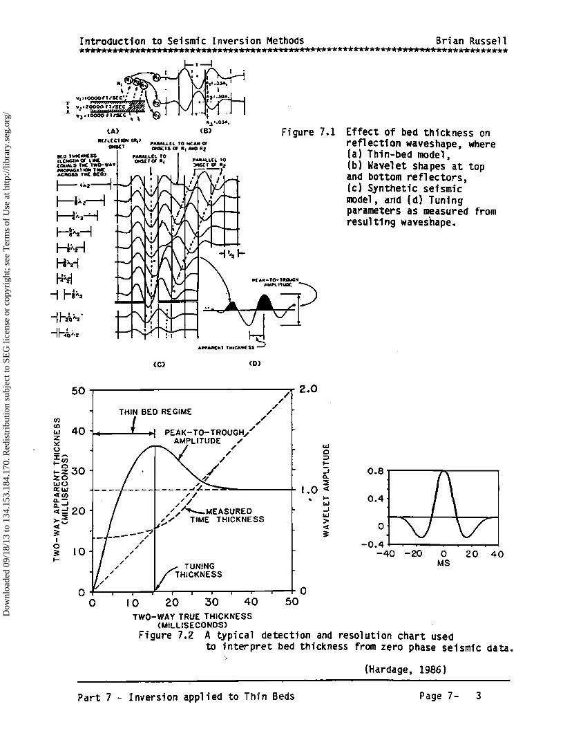
Figure 7.1 is taken from Widess' paper and shows the synthetic section as the thickness of the layer decreases from twice the dominant period of the

wavelet to 1/ZOth of the dominant period. (Note that what is refertea to as a

wavelength in his plot i s actual ly twice the dominant period). A few important points can be noted from Figure 7.1. First, the wavelets start interfering with eack other at a thickness just below two dominant periods, but remain Clistinguishable down to about one period.

Part 7 - Inversion applied to Thin Beds Page 7- g

Dow

nloa

ded

09/1

8/13

to 1

34.1

53.1

84.1

70. R

edis

trib

utio

n su

bjec

t to

SEG

lice

nse

or c

opyr

ight

; see

Ter

ms

of U

se a

t http

://lib

rary

.seg

.org

/


PI•OPAGA ! ION I NdC ACnOSS TK arO) .

•'------ •).z _1 I

--t

Figure 7.1 Effect of bed thickness on reflection waveshape, where (a) Thin-bed model, (b) Wavelet shapes at top and bottom re fl ectors, (c) Synthetic seismic model, anU (d) Tuning parameters as measured from resul ting waveshape.

(C) (D)

5O , ,.

THIN BED REGIME

J PEAK-TO-TROUGH/ AMPLITUDE

2.0

1.0 <

0.8

0.4

/ \ -0.4 ,• i . . . . .

-40 0 20 40 MS

TWO-WAY TRUE THICKNESS (MILLISECONDS)

Figure 7.2 A typical detection and resolution cha•t used to interpret bed thickness from zero phase seismic data.

('Hardage, 1986 ) . .. _ i i ,, , i _ - - - -_- - _ - _ ..... l. _

Part 7 - Inversion applied to Thin Beds Page 7- 3

Dow

nloa

ded

09/1

8/13

to 1

34.1

53.1

84.1

70. R

edis

trib

utio

n su

bjec

t to

SEG

lice

nse

or c

opyr

ight

; see

Ter

ms

of U

se a

t http

://lib

rary

.seg

.org

/


Below a thickness value of one period the wavelets Start merging into a single wavelet, and an amplitude increase is observe•. This amplitude

increase is a maximum at 1/4 period, and decreases from this point down... The

amplitude is appraoching zero at 1/•0 period, but note that the resulting waveform is a gO degree phase shifted version of the original wavelet.

A more quantitative way to measure this information is to plot the peak to trough amplitude difference and i sochron across the thin bed. This is done

in Figure 7.•, taken from Hardage (1986). This diagram quantifies what has

already been seen qualitatively the seimsic section. That is that the

amplitude is a maximum at a thickness of 1/4 the wavelet dominant period, and

also that this is the lower isochron limit. Thus, 1/4 the dominant period is considered to be the thin bed threshhold, below which it is difficult to

obtain fully resolved reflection coefficients.

7.2 In. version Camparison of T.hin Bees

ß

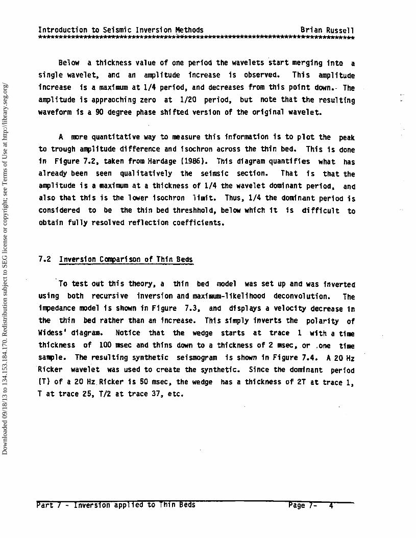
To test out this theory, a thin bed model was set up and was inverted

using both recursire inversion and maximum-likelihood aleconvolution. The

impedance model is shown in Figure 7.3, and displays a velocity decrease in

the thin bed rather than an increase. This simply inverts the polarity of Widess' diagram. Notice that the wedge starts at trace 1 with a time thickness of 100 msec and thins down to a thickness of 2 msec,.or .one time

sample. The resulting synthetic seismogram is shown in Figure 7.4. A 20 Hz

'Ricker wavelet was used to create the synthetic. Since the dominant period (T) of a 20 Hz Ricker is 50 msec, the wedge has a thickness of 2T at trace 1, T at trace 25, T/2 at trace 37, etc.

Parl• '7 - 'inverslYn 'ap'pl led 1•o Thin'- Beds ..... Page 7 --'4 '•-

Dow

nloa

ded

09/1

8/13

to 1

34.1

53.1

84.1

70. R

edis

trib

utio

n su

bjec

t to

SEG

lice

nse

or c

opyr

ight

; see

Ter

ms

of U

se a

t http

://lib

rary

.seg

.org

/


lOO

200

3OO

400

500

4 8 12 16 20 24 28 32 36 40 44 48

ß

Figure 7.3 True impedance from wedge model.

o

lOO

200

.

300

ß

400

500

Figure 7.4 Wedge model reflectivity convol ved with 20 HZ Ricker wavelet.

Part 7 - Inversion applied to Thin BeUs Page 7- 5

Dow

nloa

ded

09/1

8/13

to 1

34.1

53.1

84.1

70. R

edis

trib

utio

n su

bjec

t to

SEG

lice

nse

or c

opyr

ight

; see

Ter

ms

of U

se a

t http

://lib

rary

.seg

.org

/


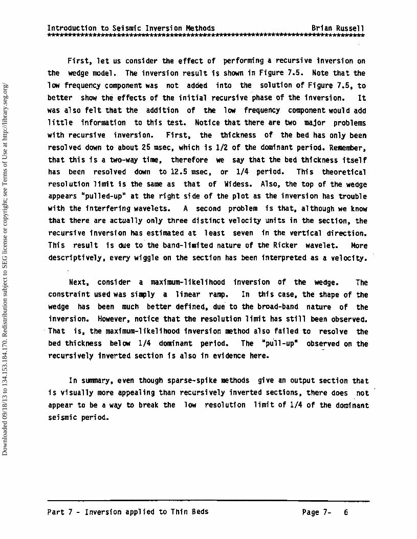
First, let us consider the effect of performing a recursire inversion on

the wedge model. The inversion result is shown in Figure 7.5. Note that the

low frequency component was not added into the solution of Figure 7.5, to better show the effects of the initial recursire phase of the inversion. It

was also felt that the addition of the low frequency component would ado

little information to this test. Notice that there'are two major problems

with recursire inversion.. First, the thickness of the beU has only been

resolved down to about 25 msec, which is 1/2 of the dominant period. Remember,

that this is a two-way time, therefore we say that the bed thickness itself

has been resolved down to 12.5 msec, or 1/4 period. This theoretical

resolution limit is the same as that of Widess. Also, the top of the weUge appears "pulled-up" at the right side of the plot as the inversion has trouble

with the interfering wavelets. A second problem is that, although we know

that there are actually only three distinct velocity units in the section, the recursire inversion has estimate• at least seven in the vertical =irection.

ß

This result is Uue to the banu-limited nature of the Ricker wavelet. More

Uescriptively, every wiggle on the section has been interpreted as a velocity. ß

Next, consider a maximum-likelihood inversion of the weOge. The

constraint used was simply a linear ramp. In this case, the shape of the ß

wedge has been much better defined, due to the broad-band nature of the

inversion. However, notice that the resolution limit has still been observeU.

That is, the maximum-likelihood inversion method also failed to resolve the

bed thickness below 1/4 dominant period. The "pUll-up" observed on the recursively inverted section is also in evidence here.

In summary, even though sparse-spike methods give an output section that

is visually more appealing than recursively inverted sections, there does not

appear to be a way to break the low resolution limit of 1/4 of the dominant

se i smi c peri od.

Part 7 - Inversion applied to Thin Beds

_ i _ i mk

Page 7- 6

Dow

nloa

ded

09/1

8/13

to 1

34.1

53.1

84.1

70. R

edis

trib

utio

n su

bjec

t to

SEG

lice

nse

or c

opyr

ight

; see

Ter

ms

of U

se a

t http

://lib

rary

.seg

.org

/

Introduction to Seismic Inversi.on Methods Brian Russell

4 8 12 16 20 24 28 32 36 40 44 48 o

300-

400.

Figure 7.5 Recursive inversion of wedge model shown in Figure 7.4.

4 8 12 16 20 24 28 32 36 40 44 48 ' ' • i ' ' I i

100 -. .................

300

400

500 ,, .

Figure 7.6 Maximum-likelihood derived impedance of wedge moUel shown i n Figure 7.4.

Part 7 - Inversion applied to Thin Beds - 7

Dow

nloa

ded

09/1

8/13

to 1

34.1

53.1

84.1

70. R

edis

trib

utio

n su

bjec

t to

SEG

lice

nse

or c

opyr

ight

; see

Ter

ms

of U

se a

t http

://lib

rary

.seg

.org

/

introduction to seismic inversion methods || 7. part 7 - inversion applied to thin-beds

Documents