introduction to reliability and sensitivity...

Introduction to Reliability and Sensitivity Analysis Armen Der KiureghianUC Berkeley

OpenSees WorkshopUC BerkeleyAugust 23, 2011

Outline

Formulation of structural reliability problem Solution methods Uncertainty propagation Response sensitivity analysis Sensitivity/importance measures Methods implemented in OpenSees Example – probabilistic pushover analysis Stochastic nonlinear dynamic analysis Example – fragility analysis of hysteretic system Summary and conclusions

Formulation of structural reliability

Vector of random variables

Distribution of X

Failure domain

Failure probability∫Ω

=

Ω

=

x

xx

x

X

X

x

X

dfp

f

X

X

f

n

)(

)(

1

x1

x2

fX(x) ΩX

pf

Formulation of structural reliability

Component reliability problem

0)( ≤≡Ω xx g

System reliability problem

≤≡Ω∈

0)(xx ik Ci

gk

)(),( xx igg limit-state functions (must be continuously differentiable)

e.g., failure due to excessive ith story drift)()( xx icrig δ−δ=

Solution by First-Order Reliability Method (FORM)

( )β−Φ≅

∇∇

−=

⋅=β

≤=

→=

=

fp

GG

G

Gg

*)()(

indexy reliabilit

)(minarg

)()(),(

*

*

uu

u

uuα

uα

0uuu

uxxTu

x1

x2

fX(x) ΩX

u1

u2

ΩU β

αu*

FORMapprox

Der Kiureghian, A. (2005). First- and second-order reliability methods. Chapter 14 in Engineering design reliability handbook, E. Nikolaidis, D. M. Ghiocel and S. Singhal, Edts., CRC Press, Boca Raton, FL.

cte=ϕ )(u

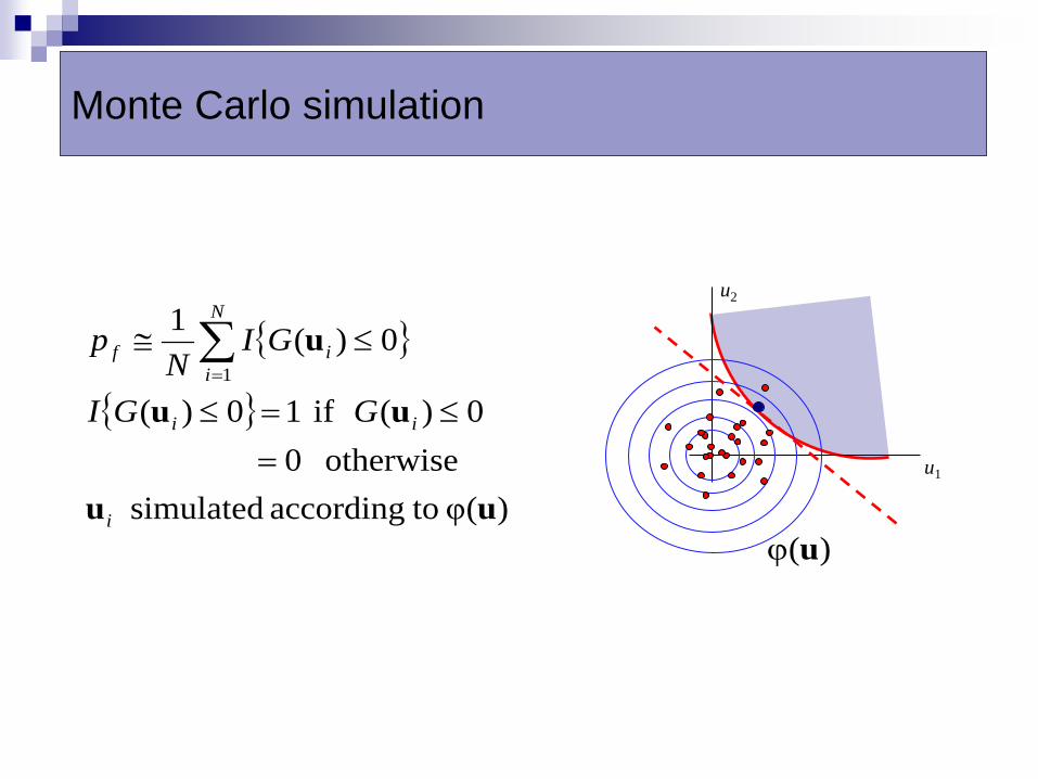
Monte Carlo simulation

)(φ toaccording simulated otherwise 0

0)( if 10)(

0)(11

uu

uu

u

i

ii

N

iif

GGI

GIN

p

=≤=≤

≤≅ ∑=

u1

u2

)(uϕ

Solution by importance sampling

)( toaccording simulated

)()(0)(1

1

uu

uuu

h

hGI

Np

i

i

iN

iif ∑

=

≤≅

u1

u2

)(uh

)(uϕ

Uncertainty propagation

response quantity of interest

∂∂

∂∂

=∇

Σ

∇∇≅

≅

=

nxxδδδ

δδσ

)(δμ

)(δδ

1

T2δ

δ

X

XX

X

XXXX

X

M

Σ

M

X

mean vector

covariance matrix

gradient row-vector

First-order approximations:

Response sensitivity analysis

For both FORM and FOSM, we needix∂

δ∂ )(x

Available methods in OpenSees:

Finite difference

Direct Differentiation Method (DDM)Differentiate equations of motion and solve for response derivative equations as adjoint to the equations of motion. Equations for the response derivative are linear, even for nonlinear response.

DDM is more stable, accurate and efficient than finite difference.

Zhang, Y., and A. Der Kiureghian (1993). Dynamic response sensitivity of inelastic structures. Comp. Methods Appl. Mech. Engrg., 108(1), 23-36.

Haukaas, T., and A. Der Kiureghian (2005). Parameter sensitivity and importance measures in nonlinear finite element reliability analysis. J. Engineering Mechanics, ASCE, 131(10): 1013-1026.

Brief on DDM

Linear static problems:

∂∂

−∂∂

=∂∂

∂∂

=∂∂

+∂∂

=

− δKPKδ

PδKδK

xPxδxK

xxx

xxx

1

)()()(

Brief on DDM

Nonlinear static problems:

Ω∂

∂=

∂∂

=∂

∂=

∂∂

−∂∂

=∂∂

∂∂

=∂

∂+

∂∂

∂∂

=

∑∫

−

−

dx

xx

x

xx

xxx

xxx

xx

xx

e

T

t

t

ε

vσvBδRδδRK

δRPKδ

PδRδδδR

xPδR

fixed

1

1

),()(),(

matrix stiffness tangent ),(

),(

),(),(

)()),((

Sensitivity/Importance measures

FOSM:

FORM:

valuesstdev of importancey reliabilit

smean value of importancey reliabilit

variables of importance relative variables of importance relative

)(

=

σσ∂β∂

=

=

σµ∂β∂

=

=

=

σ∂δ∂

ii

ii

iix

η

δ

Xγuα

x

Haukaas, T., and A. Der Kiureghian (2005). Parameter sensitivity and importance measures in nonlinear finite element reliability analysis. J. Engineering Mechanics, ASCE, 131(10): 1013-1026.

Methods implemented in OpenSees

Propagation of uncertainty:

Estimate second moments of response

First-Order Second-Moment (FOSM)Monte Carlo sampling (MCS)

First-Order Reliability Method (FORM)Importance Sampling (IS)Second-Order Reliability Method (SORM)

The Direct Differentiation Method (DDM)Finite Difference scheme (FD)

• Mean• Standard deviation• Correlation• Parameter importanceat mean point

• “Design point”• Probability of failure• Parameter importance/ sensitivity measures

•

(Used in FOSM and FORM analysis)

parameter response

∂∂

Reliability analysis:

Estimate probability of events defined in terms of limit-state functions

Response sensitivity analysis:Determine derivative of response with respect to input or structural properties

320 random variables

The I-880 Testbed Bridge

2590 mm

2440 mm

R 1170 mm

127 mm

51 mm

36 - 43 mm bars

8 - 16 mm bars

Hoop Transverse Reinforcement 25 mm bars at 102 mm on center

9.3 m

15.6 m

1.7 m1.7 m

12 - 35 mm bars(6 each side)

8 - 11 mm bars

32 - 57 mm bars

20 - 44 mm bars

Section 1

Section 2

Section 1

Section 2

g1 = uo - u(λo)g2 = λo - λ(uo)g3 = u(20% tangent) - uog4 = λ(20% tangent) - λ o

First-Order Second-Moment Analysis

Second-moment response statistics for u(λo)

Second-moment response statistics for λ(uo)

FORM Analysis, g1, λo=0.20

Parameter Importance 1 -0.603 Element 141 σy2 -0.538 Element 142 σy3 -0.280 Element 151 σy4 0.240 Element 142 f'c5 0.232 Element 142 εcu6 -0.188 Element 152 σy7 -0.177 Element 1502 E8 0.135 Element 142 f'c9 -0.122 Element 1602 E

10 -0.100 Element 161 σy11 0.091 Element 141 f'c12 0.083 Element 152 f'c13 -0.073 Element 141 b14 -0.058 Element 142 εc15 -0.056 Element 162 σy16 -0.048 Element 142 b17 0.046 Element 142 εc18 0.040 Element 152 εcu19 -0.040 Element 1502 E20 0.040 Element 152 f'c21 -0.032 Element 141 E22 0.031 Element 162 f'c23 0.029 Element 151 f'c24 -0.027 Node 14002 y-crd.25 0.026 Element 141 εc26 0.026 Node 14005 y-crd.27 -0.023 Element 1602 E28 -0.022 Element 142 E29 -0.022 Element 151 b30 0.021 Element 162 εc

171 172

161 162

151 152

141 142

g1 = 0.35 - u(λ=0.2)

FORM Analysis, g2, uo=0.30

Continuity of response derivative

FORM Analysis, g3 and g4

Haukaas, T., and A. Der Kiureghian (2007). Methods and object-oriented software for FE reliability and sensitivity analysis with application to a bridge structure. Journal of Computing in Civil Engineering, ASCE, 21(3):151-163.

g3 = u(20% tangent) - uog4 = λ(20% tangent) - λ o

21

it1i-t

1+itt

si(t) normalized response of a time-dependent filter

q(ti)ui

Stochastic nonlinear dynamic analysis

Spectral nonstationarityTemporal nonstationarity

Stochasticity

Representation of stochastic ground motion

usu )()()()(),(1

ttqutstqtA n

i ii == ∑ =

22

Representation of stochastic ground motion

usu )()()()(),(1

ttqutstqtA n

i ii == ∑ =


-10.0

-5.0

0.0

5.0

10.0

0 10 20 30 40

time(s)

acc (m

/s2)

Rezaeian, S. and A. Der Kiureghian (2009). Simulation of synthetic ground motions for specified earthquake and site characteristics. Earthquake Engineering & Structural Dynamics, 39:1155-1180.

23

xtX =),( u

1u

2u

*u

),( txa),(β tx


[ ]),(Pr utXx ≤ tail probability for threshold x at time t

Solution of the above problem by FORM leads to identification of a Tail-Equivalent Linear System (TELS).

TELS is solved by linear random vibration methods to obtain response statistics of interest, e.g., distribution of extreme peak response, fragility curve.

Fujimura, K., and A. Der Kiureghian (2007). Tail-equivalent linearization method for nonlinear random vibration. Probabilistic Engineering Mechanics, 22:63-76.

24

Node 1

Node 2

Node 5

Node 4

Node 3

Node 6

m=3.0×104kg for all nodes

k0=5.5×104kN/m

k0=2.0×104kN/m

k0=6.5×104kN/m

k0=4.0×104kN/m

k0=7.0×104kN/m

k0=7.5×104kN/m

Application to MDOF hysteretic system

Disp. (m)6th story

-0.04

0.04-300

300

0.0

Force (kN)

Disp. (m)1st story

-0.04 0.04-1000

1000

0.0

Force (kN)

Smooth bilinear hysteresis model

25

Fragility curves for story drifts

1.0E-5

1.0E-4

1.0E-3

1.0E-2

1.0E-1

1.0E+0

0 0.5 1 1.5 21.0E-5

1.0E-4

1.0E-3

1.0E-2

1.0E-1

1.0E+0

0 0.5 1 1.5 2 2.5

Sa(T = 0.576s, ζ = 0.05) in g’s Sa(T = 0.576s, ζ = 0.05) in g’s

Pr[x

<max

t∈(0

,20)

|X(t)

|]

1% drift

2%

3%

1%2%

3%

First story Sixth story

Der Kiureghian, A., and K. Fujimura (2009). Nonlinear stochastic dynamic analysis for performance-based earthquake engineering. Earthquake Engineering and Structural Dynamics, 38:719-738.

26

Summary and conclusions

Reliability analysis requires specification of uncertain quantities, their distributions, and definition of performance via limit-state function(s). It provides probability of exceeding specified performance limit(s).

Uncertainty propagation provides first-order approximation of mean, variance and correlations of response quantities.

Sensitivity and importance measures provide insight into the relative importance of variables and parameters.

Stochastic dynamic analysis is performed via tail-equivalent linearization. TELM can be used to generate fragility functions (e.g., in lieu of performing IDAs).

introduction to reliability and sensitivity...

Documents