introduction to mesoscale meteorology: part...
TRANSCRIPT
Introduction to Mesoscale Meteorology: Part II
Jeremy A. Gibbs
School of Meteorology
January 15, 2015
1 / 70
Overview
Administrative Follow-UpHomeworkExamsTerm Project
Introduction to Mesoscale, ContinuedSynoptic ScaleMesoscaleClassification of ScalesDefinition of Scales via Scale Analysis on Equations of MotionSummary
2 / 70
Homework
Homework 1
I Distributed on February 3rd
I Due on February 17th
Homework 2
I Distributed on March 3rd
I Due on March 24th (extra week for Spring Break)
Homework 3
I Distributed on April 9th
I Due on April 23rd
I The dates for this homework may change slightly
3 / 70
Exams
Exam 1
I In class on Tuesday, February 24th from 11:30 am - 12:45 pm
I This will cover the first three chapters of material (intro,mountain waves, boundary layer)
Exam 2
I Time to be announced later
I This will cover the fourth chapter of material (convection,single/multi-cell storms, squall lines, supercells, tornadoes,etc.)
Final Exam
I Thursday May 7 in NWC 5600 from 10:30 am - 12:30 pm
4 / 70

Term Project
I Project will be a review of a mesoscale topic of your choice
I Distributed on Tuesday, March 10 - more info then
I Due on the last day of class (April 30th)
5 / 70
Synoptic Scale
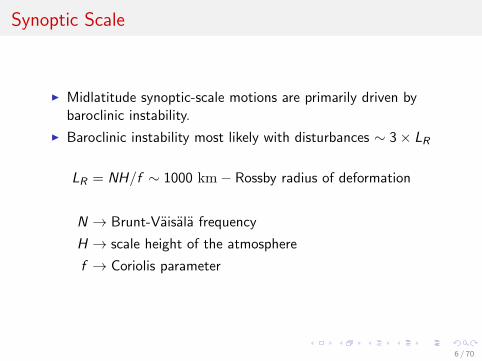
I Midlatitude synoptic-scale motions are primarily driven bybaroclinic instability.
I Baroclinic instability most likely with disturbances ∼ 3× LR
LR = NH/f ∼ 1000 km− Rossby radius of deformation
N → Brunt-Vaisala frequency
H → scale height of the atmosphere
f → Coriolis parameter
6 / 70
Synoptic Scale
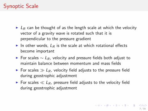
I LR can be thought of as the length scale at which the velocityvector of a gravity wave is rotated such that it isperpendicular to the pressure gradient
I In other words, LR is the scale at which rotational effectsbecome important
I For scales ∼ LR , velocity and pressure fields both adjust tomaintain balance between momentum and mass fields
I For scales � LR , velocity field adjusts to the pressure fieldduring geostrophic adjustment
I For scales � LR , pressure field adjusts to the velocity fieldduring geostrophic adjustment
7 / 70
Synoptic Scale
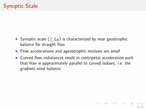
I Synoptic scale (& LR) is characterized by near geostrophicbalance for straight flow
I Flow accelerations and ageostrophic motions are small
I Curved flow imbalances result in centripetal acceleration suchthat flow is approximately parallel to curved isobars, i.e. thegradient wind balance.
8 / 70
Mesoscale
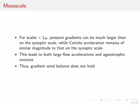
I For scales < LR , pressure gradients can be much larger thanon the synoptic scale, while Coriolis acceleration remains ofsimilar magnitude to that on the synoptic scale
I This leads to both large flow accelerations and ageostrophicmotions
I Thus, gradient wind balance does not hold
9 / 70
Mesoscale
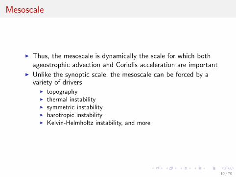
I Thus, the mesoscale is dynamically the scale for which bothageostrophic advection and Coriolis acceleration are important
I Unlike the synoptic scale, the mesoscale can be forced by avariety of drivers
I topographyI thermal instabilityI symmetric instabilityI barotropic instabilityI Kelvin-Helmholtz instability, and more
10 / 70
Mesoscale
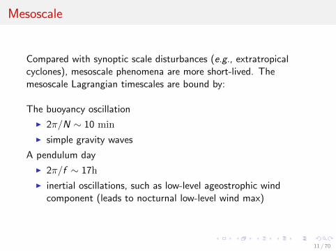
Compared with synoptic scale disturbances (e.g., extratropicalcyclones), mesoscale phenomena are more short-lived. Themesoscale Lagrangian timescales are bound by:
The buoyancy oscillation
I 2π/N ∼ 10 min
I simple gravity waves
A pendulum day
I 2π/f ∼ 17h
I inertial oscillations, such as low-level ageostrophic windcomponent (leads to nocturnal low-level wind max)
11 / 70
A Rough Definition
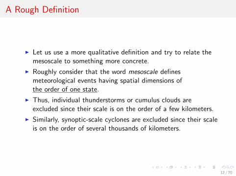
I Let us use a more qualitative definition and try to relate themesoscale to something more concrete.
I Roughly consider that the word mesoscale definesmeteorological events having spatial dimensions ofthe order of one state.
I Thus, individual thunderstorms or cumulus clouds areexcluded since their scale is on the order of a few kilometers.
I Similarly, synoptic-scale cyclones are excluded since their scaleis on the order of several thousands of kilometers.
12 / 70
Classification of Scales
13 / 70
Classification of Scales
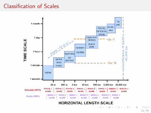
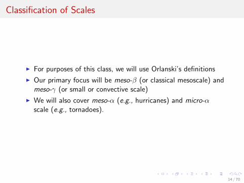
I For purposes of this class, we will use Orlanski’s definitions
I Our primary focus will be meso-β (or classical mesoscale) andmeso-γ (or small or convective scale)
I We will also cover meso-α (e.g., hurricanes) and micro-αscale (e.g., tornadoes).
14 / 70
Time Scales
Some temporal scales in the atmosphere are obvious.
I diurnal cycle
I annual cycle
I inertial oscillation period - due to Earth’s rotation, the Coriolisparameter f
I advective time scale - time taken to advect over certaindistance
15 / 70
Space Scales
Some space scales in the atmosphere are obvious.
I global - related to earth’s radius
I scale height of the atmosphere - related to the total mass ofthe atmosphere and gravity
I scale of fixed geographical features - mountain height, width,width of continents, oceans, lakes
16 / 70
Scale Analysis
Scale analysis is a very useful method for establishing theimportance of various processes in the atmosphere and terms inthe governing equations.
Based on the relative importance of these processes/terms, we candeduce much of the behavior of motion at such scales.
17 / 70
Scale Analysis
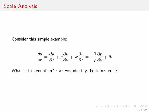
Consider this simple example:
du
dt=∂u
∂t+ u
∂u
∂x+ w
∂u
∂z= −1
ρ
∂p
∂x+ fv
What is this equation? Can you identify the terms in it?
18 / 70
Scale Analysis
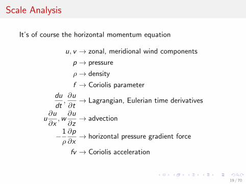
It’s of course the horizontal momentum equation
u, v → zonal, meridional wind components
p → pressure
ρ→ density
f → Coriolis parameter
du
dt,∂u
∂t→ Lagrangian, Eulerian time derivatives
u∂u
∂x,w
∂u
∂z→ advection
−1
ρ
∂p
∂x→ horizontal pressure gradient force
fv → Coriolis acceleration
19 / 70
Scale Analysis
du
dt=∂u
∂t+ u
∂u
∂x+ w
∂u
∂z= −1
ρ
∂p
∂x+ fv
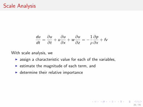
With scale analysis, we
I assign a characteristic value for each of the variables,
I estimate the magnitude of each term, and
I determine their relative importance
20 / 70
Scale Analysis
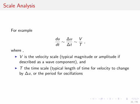
For example
du
dt∼ ∆u
∆t∼ V
T,
where ,
I V is the velocity scale (typical magnitude or amplitude ifdescribed as a wave component), and
I T the time scale (typical length of time for velocity to changeby ∆u, or the period for oscillations
21 / 70
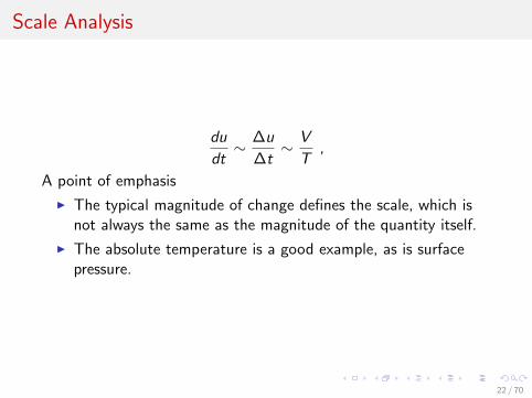
Scale Analysis
du
dt∼ ∆u
∆t∼ V
T,
A point of emphasis
I The typical magnitude of change defines the scale, which isnot always the same as the magnitude of the quantity itself.
I The absolute temperature is a good example, as is surfacepressure.
22 / 70
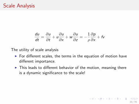
Scale Analysis
du
dt=∂u
∂t+ u
∂u
∂x+ w
∂u
∂z= −1
ρ
∂p
∂x+ fv
The utility of scale analysis
I For different scales, the terms in the equation of motion havedifferent importance.
I This leads to different behavior of the motion, meaning thereis a dynamic significance to the scale!
23 / 70
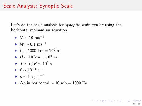
Scale Analysis: Synoptic Scale
Let’s do the scale analysis for synoptic scale motion using thehorizontal momentum equation
I V ∼ 10 ms−1
I W ∼ 0.1 ms−1
I L ∼ 1000 km = 106 m
I H ∼ 10 km = 104 m
I T ∼ L/V ∼ 105 s
I f ∼ 10−4 s−1
I ρ ∼ 1 kgm−3
I ∆p in horizontal ∼ 10 mb = 1000 Pa
24 / 70
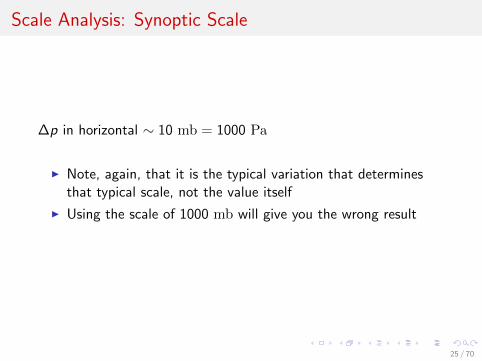
Scale Analysis: Synoptic Scale
∆p in horizontal ∼ 10 mb = 1000 Pa
I Note, again, that it is the typical variation that determinesthat typical scale, not the value itself
I Using the scale of 1000 mb will give you the wrong result
25 / 70
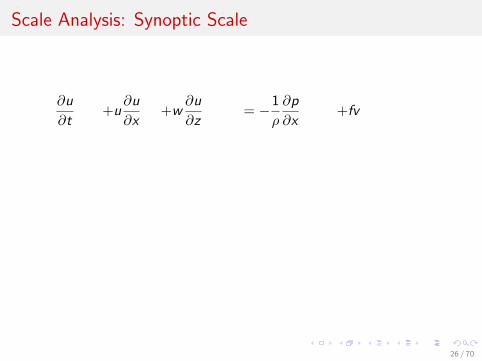
Scale Analysis: Synoptic Scale
∂u
∂t+u
∂u
∂x+w
∂u
∂z= −1
ρ
∂p
∂x+fv
26 / 70
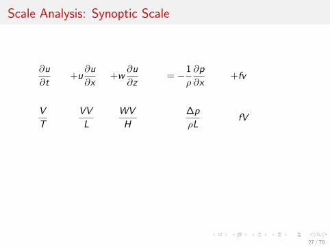
Scale Analysis: Synoptic Scale
∂u
∂t+u
∂u
∂x+w
∂u
∂z= −1
ρ
∂p
∂x+fv
V
T
VV
L
WV
H
∆p
ρLfV
27 / 70
Scale Analysis: Synoptic Scale
∂u
∂t+u
∂u
∂x+w
∂u
∂z= −1
ρ
∂p
∂x+fv
V
T
VV
L
WV
H
∆p
ρLfV
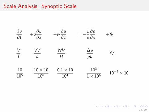
10
10510× 10
1060.1× 10
104103
1× 10610−4 × 10
28 / 70
Scale Analysis: Synoptic Scale
∂u
∂t+u
∂u
∂x+w
∂u
∂z= −1
ρ
∂p
∂x+fv
V
T
VV
L
WV
H
∆p
ρLfV
10
10510× 10
1060.1× 10
104103
1× 10610−4 × 10
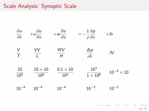
10−4 10−4 10−4 10−3 10−3
29 / 70
Scale Analysis: Synoptic Scale
∂u
∂t+u
∂u
∂x+w
∂u
∂z= −1
ρ
∂p
∂x+fv
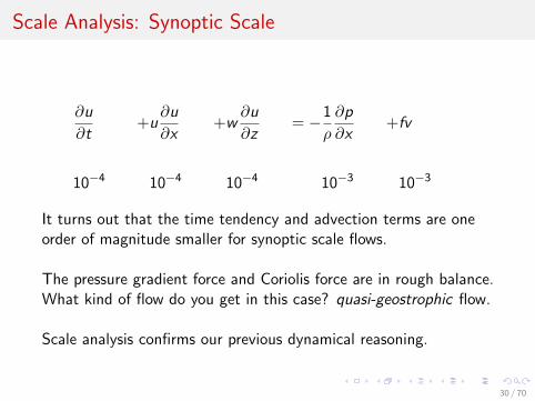
10−4 10−4 10−4 10−3 10−3
It turns out that the time tendency and advection terms are oneorder of magnitude smaller for synoptic scale flows.
The pressure gradient force and Coriolis force are in rough balance.What kind of flow do you get in this case? quasi-geostrophic flow.
Scale analysis confirms our previous dynamical reasoning.
30 / 70
Scale Analysis: Synoptic Scale
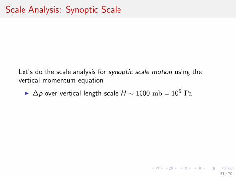
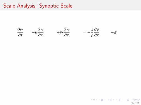
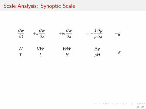
Let’s do the scale analysis for synoptic scale motion using thevertical momentum equation
I ∆p over vertical length scale H ∼ 1000 mb = 105 Pa
31 / 70
Scale Analysis: Synoptic Scale
∂w
∂t+u
∂w
∂x+w
∂w
∂z= −1
ρ
∂p
∂z−g
32 / 70
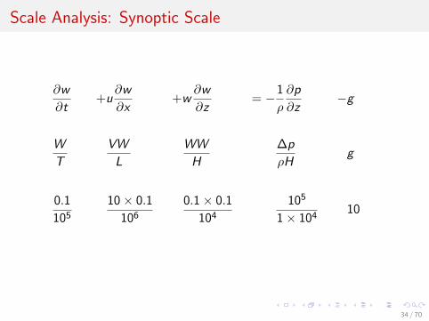
Scale Analysis: Synoptic Scale
∂w
∂t+u
∂w
∂x+w
∂w
∂z= −1
ρ
∂p
∂z−g
W
T
VW
L
WW
H
∆p
ρHg
33 / 70
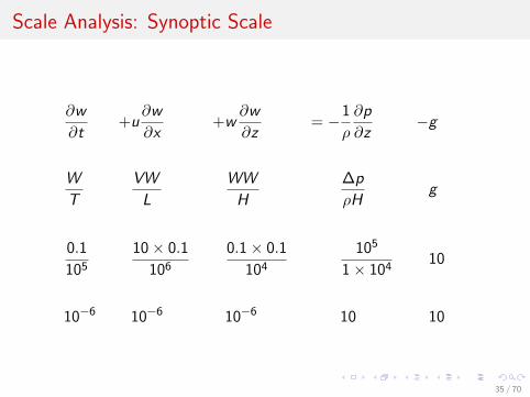
Scale Analysis: Synoptic Scale
∂w
∂t+u
∂w
∂x+w
∂w
∂z= −1
ρ
∂p
∂z−g
W
T
VW
L
WW
H
∆p
ρHg
0.1
10510× 0.1
1060.1× 0.1
104105
1× 10410
34 / 70
Scale Analysis: Synoptic Scale
∂w
∂t+u
∂w
∂x+w
∂w
∂z= −1
ρ
∂p
∂z−g
W
T
VW
L
WW
H
∆p
ρHg
0.1
10510× 0.1
1060.1× 0.1
104105
1× 10410
10−6 10−6 10−6 10 10
35 / 70
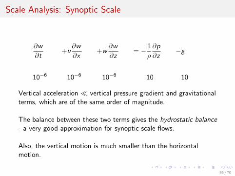
Scale Analysis: Synoptic Scale
∂w
∂t+u
∂w
∂x+w
∂w
∂z= −1
ρ
∂p
∂z−g
10−6 10−6 10−6 10 10
Vertical acceleration � vertical pressure gradient and gravitationalterms, which are of the same order of magnitude.
The balance between these two terms gives the hydrostatic balance- a very good approximation for synoptic scale flows.
Also, the vertical motion is much smaller than the horizontalmotion.
36 / 70
Scale Analysis: Synoptic Scale
We saw a good example of horizontal scale determining thedynamics of motion!
In summary, synoptic (and up) scale flows are
I quasi-two-dimensional (because w << u )
I hydrostatic (we can see it by performing scale analysis forvertical equation of motion)
I Coriolis force is a dominant term in the equation of motionand it is in rough balance with the PGF
I the flow is quasi-geostrophic
37 / 70
Scale Analysis: Mesoscale
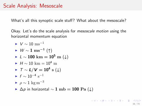
What’s all this synoptic scale stuff? What about the mesoscale?
Okay. Let’s do the scale analysis for mesoscale motion using thehorizontal momentum equation
I V ∼ 10 ms−1
I W ∼ 1 ms−1 (↑)
I L ∼ 100 km = 105 m (↓)
I H ∼ 10 km = 104 m
I T ∼ L/V = 104 s (↓)
I f ∼ 10−4 s−1
I ρ ∼ 1 kgm−3
I ∆p in horizontal ∼ 1 mb = 100 Pa (↓)
38 / 70
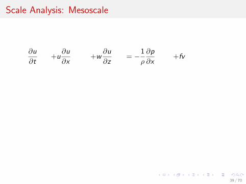
Scale Analysis: Mesoscale
∂u
∂t+u
∂u
∂x+w
∂u
∂z= −1
ρ
∂p
∂x+fv
39 / 70
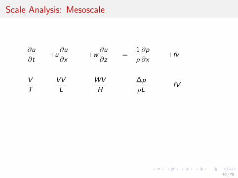
Scale Analysis: Mesoscale
∂u
∂t+u
∂u
∂x+w
∂u
∂z= −1
ρ
∂p
∂x+fv
V
T
VV
L
WV
H
∆p
ρLfV
40 / 70
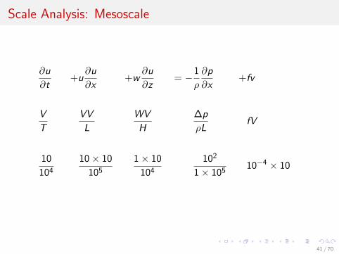
Scale Analysis: Mesoscale
∂u
∂t+u
∂u
∂x+w
∂u
∂z= −1
ρ
∂p
∂x+fv
V
T
VV
L
WV
H
∆p
ρLfV
10
10410× 10
1051× 10
104102
1× 10510−4 × 10
41 / 70
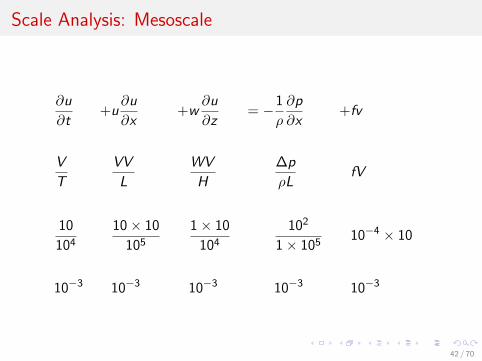
Scale Analysis: Mesoscale
∂u
∂t+u
∂u
∂x+w
∂u
∂z= −1
ρ
∂p
∂x+fv
V
T
VV
L
WV
H
∆p
ρLfV
10
10410× 10
1051× 10
104102
1× 10510−4 × 10
10−3 10−3 10−3 10−3 10−3
42 / 70
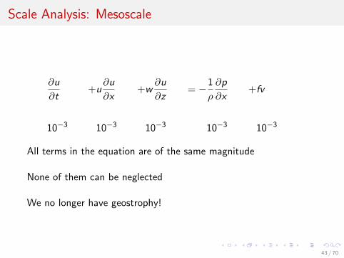
Scale Analysis: Mesoscale
∂u
∂t+u
∂u
∂x+w
∂u
∂z= −1
ρ
∂p
∂x+fv
10−3 10−3 10−3 10−3 10−3
All terms in the equation are of the same magnitude
None of them can be neglected
We no longer have geostrophy!
43 / 70
Scale Analysis: Mesoscale
Let’s do the scale analysis for mesoscale motion using the verticalmomentum equation
I The hydrostatic approximation is still reasonable for themesoscale
44 / 70
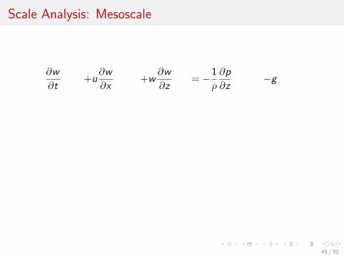
Scale Analysis: Mesoscale
∂w
∂t+u
∂w
∂x+w
∂w
∂z= −1
ρ
∂p
∂z−g
45 / 70
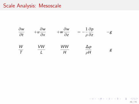
Scale Analysis: Mesoscale
∂w
∂t+u
∂w
∂x+w
∂w
∂z= −1
ρ
∂p
∂z−g
W
T
VW
L
WW
H
∆p
ρHg
46 / 70
Scale Analysis: Mesoscale
∂w
∂t+u
∂w
∂x+w
∂w
∂z= −1
ρ
∂p
∂z−g
W
T
VW
L
WW
H
∆p
ρHg
1
10410× 1
1051× 1
104105
1× 10410
47 / 70
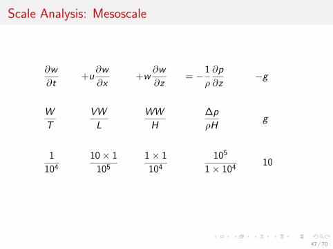
Scale Analysis: Mesoscale
∂w
∂t+u
∂w
∂x+w
∂w
∂z= −1
ρ
∂p
∂z−g
W
T
VW
L
WW
H
∆p
ρHg
1
10410× 1
1051× 1
104105
1× 10410
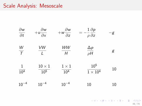
10−4 10−4 10−4 10 10
48 / 70
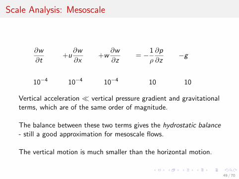
Scale Analysis: Mesoscale
∂w
∂t+u
∂w
∂x+w
∂w
∂z= −1
ρ
∂p
∂z−g
10−4 10−4 10−4 10 10
Vertical acceleration � vertical pressure gradient and gravitationalterms, which are of the same order of magnitude.
The balance between these two terms gives the hydrostatic balance- still a good approximation for mesoscale flows.
The vertical motion is much smaller than the horizontal motion.
49 / 70
Scale Analysis: Mesoscale
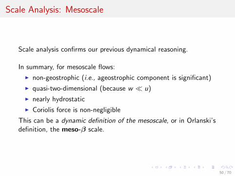
Scale analysis confirms our previous dynamical reasoning.
In summary, for mesoscale flows:
I non-geostrophic (i.e., ageostrophic component is significant)
I quasi-two-dimensional (because w � u)
I nearly hydrostatic
I Coriolis force is non-negligible
This can be a dynamic definition of the mesoscale, or in Orlanski’sdefinition, the meso-β scale.
50 / 70
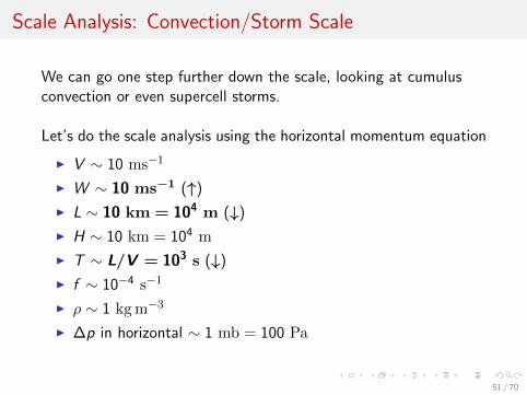
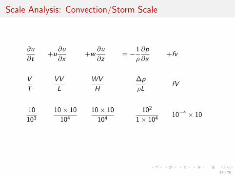
Scale Analysis: Convection/Storm Scale
We can go one step further down the scale, looking at cumulusconvection or even supercell storms.
Let’s do the scale analysis using the horizontal momentum equation
I V ∼ 10 ms−1
I W ∼ 10 ms−1 (↑)
I L ∼ 10 km = 104 m (↓)
I H ∼ 10 km = 104 m
I T ∼ L/V = 103 s (↓)
I f ∼ 10−4 s−1
I ρ ∼ 1 kgm−3
I ∆p in horizontal ∼ 1 mb = 100 Pa
51 / 70
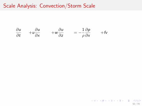
Scale Analysis: Convection/Storm Scale
∂u
∂t+u
∂u
∂x+w
∂u
∂z= −1
ρ
∂p
∂x+fv
52 / 70
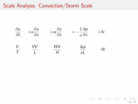
Scale Analysis: Convection/Storm Scale
∂u
∂t+u
∂u
∂x+w
∂u
∂z= −1
ρ
∂p
∂x+fv
V
T
VV
L
WV
H
∆p
ρLfV
53 / 70
Scale Analysis: Convection/Storm Scale
∂u
∂t+u
∂u
∂x+w
∂u
∂z= −1
ρ
∂p
∂x+fv
V
T
VV
L
WV
H
∆p
ρLfV
10
10310× 10
10410× 10
104102
1× 10410−4 × 10
54 / 70
Scale Analysis: Convection/Storm Scale
∂u
∂t+u
∂u
∂x+w
∂u
∂z= −1
ρ
∂p
∂x+fv
V
T
VV
L
WV
H
∆p
ρLfV
10
10310× 10
10410× 10
104102
1× 10410−4 × 10
10−2 10−2 10−2 10−2 10−3
55 / 70
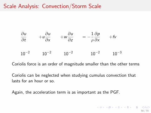
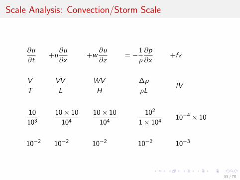
Scale Analysis: Convection/Storm Scale
∂u
∂t+u
∂u
∂x+w
∂u
∂z= −1
ρ
∂p
∂x+fv
10−2 10−2 10−2 10−2 10−3
Coriolis force is an order of magnitude smaller than the other terms
Coriolis can be neglected when studying cumulus convection thatlasts for an hour or so.
Again, the acceleration term is as important as the PGF.
56 / 70
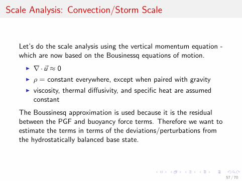
Scale Analysis: Convection/Storm Scale
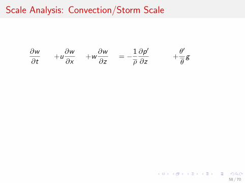
Let’s do the scale analysis using the vertical momentum equation -which are now based on the Bousinessq equations of motion.
I ∇ · ~u ≈ 0
I ρ = constant everywhere, except when paired with gravity
I viscosity, thermal diffusivity, and specific heat are assumedconstant
The Boussinesq approximation is used because it is the residualbetween the PGF and buoyancy force terms. Therefore we want toestimate the terms in terms of the deviations/perturbations fromthe hydrostatically balanced base state.
57 / 70
Scale Analysis: Convection/Storm Scale
∂w
∂t+u
∂w
∂x+w
∂w
∂z= −1
ρ
∂p′
∂z+θ′
θg
58 / 70
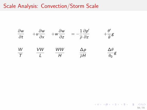
Scale Analysis: Convection/Storm Scale
∂w
∂t+u
∂w
∂x+w
∂w
∂z= −1
ρ
∂p′
∂z+θ′
θg
W
T
VW
L
WW
H
∆p
ρH
∆θ
θ0g
59 / 70
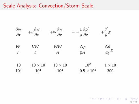
Scale Analysis: Convection/Storm Scale
∂w
∂t+u
∂w
∂x+w
∂w
∂z= −1
ρ
∂p′
∂z+θ′
θg
W
T
VW
L
WW
H
∆p
ρH
∆θ
θ0g
10
10310× 10
10410× 10
104102
0.5× 1041× 10
300
60 / 70
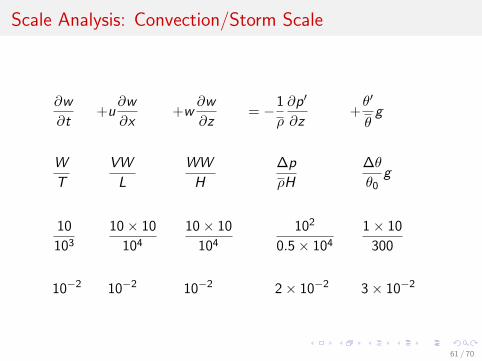
Scale Analysis: Convection/Storm Scale
∂w
∂t+u
∂w
∂x+w
∂w
∂z= −1
ρ
∂p′
∂z+θ′
θg
W
T
VW
L
WW
H
∆p
ρH
∆θ
θ0g
10
10310× 10
10410× 10
104102
0.5× 1041× 10
300
10−2 10−2 10−2 2× 10⁻² 3× 10⁻²
61 / 70
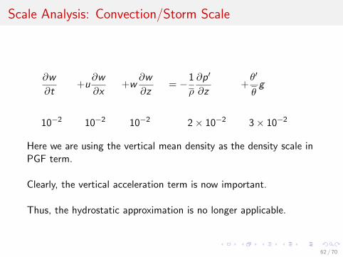
Scale Analysis: Convection/Storm Scale
∂w
∂t+u
∂w
∂x+w
∂w
∂z= −1
ρ
∂p′
∂z+θ′
θg
10−2 10−2 10−2 2× 10⁻² 3× 10⁻²
Here we are using the vertical mean density as the density scale inPGF term.
Clearly, the vertical acceleration term is now important.
Thus, the hydrostatic approximation is no longer applicable.
62 / 70
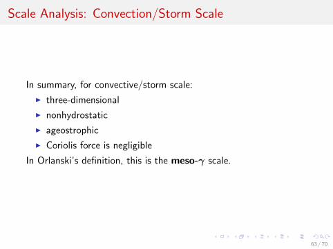
Scale Analysis: Convection/Storm Scale
In summary, for convective/storm scale:
I three-dimensional
I nonhydrostatic
I ageostrophic
I Coriolis force is negligible
In Orlanski’s definition, this is the meso-γ scale.
63 / 70
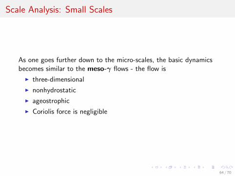
Scale Analysis: Small Scales
As one goes further down to the micro-scales, the basic dynamicsbecomes similar to the meso-γ flows - the flow is
I three-dimensional
I nonhydrostatic
I ageostrophic
I Coriolis force is negligible
64 / 70
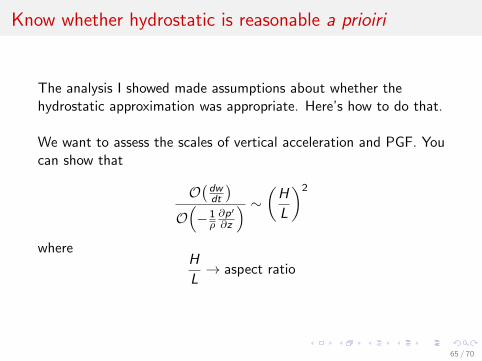
Know whether hydrostatic is reasonable a prioiri
The analysis I showed made assumptions about whether thehydrostatic approximation was appropriate. Here’s how to do that.
We want to assess the scales of vertical acceleration and PGF. Youcan show that
O(dwdt
)O(−1ρ∂p′
∂z
) ∼ (H
L
)2
whereH
L→ aspect ratio
65 / 70
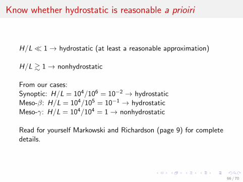
Know whether hydrostatic is reasonable a prioiri
H/L� 1→ hydrostatic (at least a reasonable approximation)
H/L & 1→ nonhydrostatic
From our cases:Synoptic: H/L = 104/106 = 10−2 → hydrostaticMeso-β: H/L = 104/105 = 10−1 → hydrostaticMeso-γ: H/L = 104/104 = 1→ nonhydrostatic
Read for yourself Markowski and Richardson (page 9) for completedetails.
66 / 70
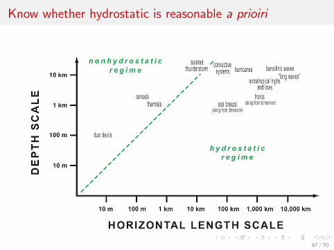
Know whether hydrostatic is reasonable a prioiri
67 / 70
Summary
There are more than one way to define the scales of weathersystems.
I Time/space scales of the system.
I Physically meaningful non-dimensional parameters (e.g.,Rossby number).
68 / 70
Summary
The most important thing to know is the key characteristicsassociated with weather systems/disturbances at each of thesescales!
Don’t get caught up in arbitrary names scientists give to thescales. Focus on physical features.
69 / 70

The End
Have a Great Weekend
70 / 70