introduction dirac operator v - harvard department of …knill/seminars/providence/ilas.pdfthe dirac...

THE DIRAC OPERATOR OF A GRAPH

OLIVER KNILL

Abstract. We discuss some linear algebra related to the Diracmatrix D of a finite simple graph G = (V,E).

1. Introduction

These are expanded preparation notes to a talk given on June 5, 2013at ILAS. References are in [4, 5, 3, 9, 2, 1, 10, 8, 6, 7, 2, 12, 11]. Itis a pleasure to thank the organizers of ILAS and especially LeslieHogben and Louis Deaett, the organizers of the matrices and graphtheory minisymposium for their kind invitation to participate.

2. Dirac operator

Given a finite simple graph G = (V,E), let Gk be the set of Kk+1

subgraphs and let G =⋃k=0 Gk be the union of these sub-simplices.

Elements in G are also called cliques in graph theory. The Diracoperator D is a symmetric v × v matrix D, where v is the cardi-nality of G. The matrix D acts on the vector space Ω = ⊕k=0Ωk,where Ωk is the space of scalar functions on Gk. An orientation ofa k-dimensional clique x ∼ Kk+1 is a choice of a permutation of its(k + 1) vertices. An orientation of the graph is a choice of ori-entations on all elements of G. We do not require the graph to beorientable; the later would require to have an orientation which iscompatible on subsets or intersections of cliques and as a triangular-ization of the Moebius strip demonstrates, the later does not alwaysexist. The Dirac matrix D : Ω → Ω is zero everywhere except forDij = ±1 if i ⊂ j or j ⊂ i and |dim(x) − dim(y)| = 1 and where thesign tells whether the induced orientations of i and j match or not.The nonnegative matrix |Dij|,when seen as an adjacency matrix, de-fines the simplex graph (G,V) of (G, V ). The orientation-dependentmatrix D is of the form D = d+ d∗, where d is a lower triangular v× vmatrix satisfying d2 = 0. The matrix d is called exterior derivative

Date: June 9, 2013.1991 Mathematics Subject Classification. Primary: 05C50,81Q10 .Key words and phrases. Linear Algebra, Graph theory, Dirac operator.

1

2 OLIVER KNILL

and decomposes into blocks dk called signed incidence matrices ingraph theory. The operator d0 is the gradient, d1 is the curl, andthe adjoint d∗0 is the divergence and div(grad(f)) = d∗0d0f restrictedto functions on vertices is the scalar Laplacian L0 = B − A, whereB is the diagonal degree matrix and A is the adjacency matrix. TheLaplace-Beltrami operator D2 = L is a direct sum of matrices Lkdefined on Ωk, the first block being the scalar Laplacian L0 acting onscalar functions. To prove d d = 0 in general, take f ∈ Ω,x ∈ Gkand compute d df(x) = d(

∑i f(xi)σ(xi)) =

∑i,j σ(i)σ(j(i)))f(xij),

where xi is the simplex with vertex i removed. Now, independentof the chosen orientations, we have σ(i)σ(j(i)) = −σ(j)σ(i(j)) be-cause permutation signatures change when the order is switched. Forexample, if x is a tetrahedron, then the xij is an edge and each ap-pears twice with opposite orientation. This just given definition ofd could be done using antisymmetric functions f(x0, . . . , xn), wheredf(x0, ..., xn+1) =

∑n+1i=0 (−1)if(x0, . . . xi, . . . , xn+1) but the use of ordi-

nary functions on simplices is more convenient to implement, comeshistorically first and works for any finite simple graph. A basis for allcohomology groups of any graph is obtained less than two dozen linesof Mathematica code without referring to any external libraries. In-stead of implementing a tensor algebra, we can use linear algebra andgraph data structures which are already hardwired into modern soft-ware. Some source code is at the end. Dirac operators obtained fromdifferent orientations are unitary equivalent - the conjugation is givenby diagonal ±1 matrices, even so choosing an orientation is like pick-ing a basis in any linear algebra setting or selecting a specific gauge inphysics. Choosing an orientation fixes a “spin” value at each vertex ofG and does not influence the spectrum of D, nor the entries of L. Likespin or color in particle physics, it is irrelevant for quantum u = iLuor wave mechanics u = −Lu and only relative orientations matter forcohomology. While the just described notions in graph theory are closeto the notions in the continuum, the discrete setup is much simpler incomparison: while in the continuum, the Dirac operator must be re-alized as a matrix-valued differential operator, it is in the discrete asigned adjacency matrix of a simplex graph.

3. Calculus

Functions on vertices V = G0 form the v0-dimensional vector spaceΩ0 of scalar functions. Functions on edges D = G1 define a v1-dimensional vector space Ω1 of 1-forms, functions on triangles forma v2-dimensional vector space Ω2 etc. The matrix d0 : Ω0 → Ω1 is

THE DIRAC OPERATOR OF A GRAPH 3

the gradient. As in the continuum, we can think of d0f as a vectorfield, a function on the edges given by d0(f(a, b)) = f(b)− f(a), thinkof the value of d0f on an edge e as a directional derivative in thedirection e. The orientation on the edges tells us in which directionthis is understood. If a vertex x is fixed and an orientation is chosenon the edges connected to x so that all arrows point away from x,then df(x, y) = f(y)− f(x), an identity which explains a bit more thename “gradient”. The matrix d1 : Ω1 → Ω2 maps a function on edgesto a function on triangles. It is called the curl because it sums upthe values of f along the boundary of the triangle and is a discrete lineintegral. As in the continuum, the “velocity orientations” chosen on theedges and the orientation of the triangle play a role for line integrals.We check that curl(grad(f)) = 0 because for every triangle the resultis a sum of 6 values which pairwise cancel. Now look at the adjointmatrices d∗0 and d∗1. The signed incidence matrix d∗0 maps a functionon edges to a function on vertices. Since it looks like a discretization ofdivergence - we count up what “goes in” or “goes out” from a vertex- we write d∗0f = div(f). We have d∗0d0 = div(grad(f)) = ∆f = L0f .The Laplacian L1 acting on one-forms would correspond to ∆F forvector fields F . We have seen already that the matrix D2 restrictedto Ω0 is the combinatorial Laplacian L0 = B − A, where B is thediagonal degree matrix and A is the adjacency matrix. The story ofmulti-variable calculus on graphs is quickly told: if C is a curve inthe graph and F a vector field, a function on the oriented edges, thenthe line integral

∫CF dr is a finite sum

∑e F (e) where e′ = 1 if the

path goes with the orientation and e′ = −1 otherwise. The functione′ on the edges of the path is the analogue of the velocity vector.The identity

∫C∇f dr = f(b)− f(a) is due to cancellations inside the

path and called the fundamental theorem of line integrals. Asurface S is a collection of triangles in G for which the boundary δSis a graph. This requires that orientations on intersections of trianglescancel; otherwise we would get a chain. Abstract simplicial complexesis the frame work in which the story is usually told but this structureneeds some mathematical maturity to be appreciated, while restrictingto calculus on graphs does not. Given a function F ∈ Ω2, define the flux∫SF dS as the finite sum

∑t∈S F (t)σ(t), where σ(t) is the sign of the

orientation of the simplex t. While δS is a chain in general, element inthe free group generated by G, the assumption that δS is a graph leadsimmediately to Stokes theorem

∫SdF dS =

∫δSF dr. If the surface

S has no boundary, then the sum is zero. An example is when S is agraph which is a triangularization of a compact orientable surface andthe triangles inherit the orientation from the continuum. The exterior

4 OLIVER KNILL

derivative dk is the block part of D mapping Ωk to Ωk+1. It satisfiesdk+1dk = 0. Stokes theorem in general assures that

∫Rdf =

∫δRf if

f is in Ωk−1 and R is a subset in Gk for which δR is a graph. Fork = 3, where R is a collection of K4 subgraphs for which the boundaryS = δR is a graph, the later has no boundary and

∫Rdf =

∫Sf is the

divergence theorem. We have demonstrated in this paragraph thattools built by Poincare allow to reduce calculus on graphs to linearalgebra. In general, replacing continuum structures by finite discreteones can reduce some analysis to combinatorics, and some topology tograph theory.

4. Cohomology

The v-dimensional vector space Ω decomposes into subspaces ⊕nk=0Ωk,where Ωk is the vector space of k-forms, functions on the set Gk ofk-dimensional simplices in G. If the dimension of Ωk is vk, thenv =

∑k=0 vk and vk is the number of k-dimensional cliques in G. The

matrices dk which appear as lower side diagonal blocks in D belongto linear maps Ωk → Ωk+1. The identity dk dk−1 = 0 for all k isequivalent to the fact that L = D2 has a block diagonal structure.The kernel Ck of dk : Ωk → Ωk+1 is called the vector space of co-cycles. It contains the image Zk−1 of d : Ωk−1 → Ωk, the vectorspace of coboundaries. The quotient space Hk(G) = Ck(G)/Zk−1(G)is called the k’th cohomology group of the graph. Its dimensionbk is called the k’th Betti number. With the clique polynomialv(x) =

∑k=0 vkx

k and the Poincare polynomial p(x) =∑

k=0 bkxk,

the Euler-Poincare formula tells that v(−1) − p(−1) = 0, we havev(1) = v and p(1) = dim(ker(D)) so that v(1)− p(1) is the number ofnonzero eigenvalues of D. Linear algebra relates the topology of thegraph with the matrix D. The proof of the Euler-Poincare formulaneeds the rank-nullity theorem vk = zk+rk, where zk = ker(dk) andrk = im(dk) as well as the formula bk = zk − rk−1 which follows fromthe definition Hk(G) = Ck(G)/Zk−1(G): the dimension of a quotientvector space is equal to the dimension of the orthogonal complement.If we add up these two equations, we get vk − vk = rk − rk−1. Thesum over k, using r0 = rn+1 = 0, telescopes to 0. We have proventhe Euler-Poincare formula. For example, if G has no tetrahe-dra, then the Euler-Poincare formula tells for a connected graph thatv − e + f = v0 − v1 + v2 = 1 − b1 + b2. If G is a triangularization ofa surface of genus g, then b2 = 1, b1 = 2g which leads to the formulav − e + f = 2 − 2g. An other example is the circular graph G = Cn,where v0 = v1 = n and b0 = b1 = 1. A constant nonzero function on


the vertices is a representative of H0(G) and a constant nonzero func-tion on the edges is a representative of H1(G). If H0(G) and Hn(G)are both one-dimensional and all other Hk(G) are trivial, the graphis called a homology sphere graph. It can be a triangularizationof the usual sphere but does not need to be as a triangularization ofthe Poincare homology sphere. For triangularizations of compact n-dimensional manifolds, we have the Poincare duality bk = bn−k, thereason being that the dual triangularization has the same Poincarepolynomial and that the dual triangularization is homotopic, leadingto the same cohomologies. This can be generalized to graph theory:whenever G has the property that there exists a dual graph which ishomotopic, then Poincare duality holds. The Betti numbers bk aresignificant because they are independent of homotopy deformations ofthe graph as we will see below. We will also see that they can be readoff as dim(ker(Lk)), so that everything is reduced to linear algebra.These ideas were all known to Poincare, who used finite-dimensionalcombinatorial theory to understand what was later called de Rhamcohomology of differential forms on compact smooth manifolds. His-torically, the setup in the continuum needed more work and Georgesde Rham was among the mathematicians who made the connection be-tween the discrete and the continuum rigorous. This paragraph shouldhave shown that the cohomology theory on graphs just needs someknowledge of linear algebra.

5. Super symmetry

The vector space Ω is the direct sum of the Bosonic subspace Ωb =⊕Ω2k and the Fermionic subspace, the span of all Ω2k+1. Let P bethe diagonal matrix which is equal to 1 on Ωb and equal to −1 on Ωf .For any linear map on A, define the super trace str(A) = tr(AP).The relations L = D2, 1 = P 2, DP + PD = 0 define what Wittencalled super symmetry in 0 dimensions. We prove here two sym-metries of the spectrum of D: the first is the symmetry λ ↔ −λ.The spectrum of D is symmetric with respect to 0 because if λ isan eigenvalue of D then −λ is an eigenvalue: if Df = λf , thenDPf = −PDf = −Pλf = −λPf . The vector Pf is the ”an-tiparticle” to the ”particle” f . Apply P again to this identity to getD(Pf) = −λ(Pf). Therefore, Pf is an eigenvector to the eigenvalue−λ. Now, we show that if λ is an eigenvalue of L to the eigenvector fthen it is also an eigenvalue of L to the eigenvector Df . If Lf = λf ,then L(Df) = DLf = Dλf = λ(Df). The two eigenvectors f,Dfbelonging to the eigenvalue λ are perpendicular if we have chosen a

6 OLIVER KNILL

basis so that Ωf and Ωb are perpendicular. The nonzero eigenvaluesin Ωb therefore pair with nonzero eigenvalues in Ωf . This leads to theidentity str(Lk) = 0 for all k > 0 and to the McKean-Singer for-mula str(e−tL) = χ(G). More generally, str(exp(f(D))) = χ(G) forany analytic function which satisfies f(0) = 0. The reason is that theeven part of exp(f(D)) can be written as g(L) and that the odd partis zero anyway because there are only zeros in the diagonal. By conti-nuity and Weierstrass, it is even true for all continuous functions. Tosummarize, we have seen that the spectrum σ(D) of D is determined

by the spectrum of L and given as ±√σ(L) as a set. Because every

nonzero eigenvalue of D comes as pair −λ, λ, each nonzero eigenvalueof L had to appear twice. The McKean-Singer symmetry gave evenmore information: the pairs belong to different subspaces Ωf and Ωb.Let us mention more anti-commutation structure which goes under thename “super symmetry”. Let A,B = AB + BA denote the anti-commutator of two square matrices A,B. We have dk, dl = 0 andDk, Dl = 2δklgk, where Dk = dk + d∗k and gk = dkd

∗k + d∗kdk. While

this again reflects the fact that D2 = L is block diagonal, it explains abit the relation with the gamma matrices γk introduced in the con-tinuum to realize the anti-commutation relations γk, γl = −2δlk andwhich was the starting point of Dirac to factor the d’Alembert Lapla-cian −∆. The first order differential operator D =

∑i γ

iδi is now thesquare root of L. Such gymnastics is not necessary in the discrete be-cause the exterior derivative and exterior bundle formalism are alreadybuilt into the graph G.

6. Hodge theory

Vectors in the kernel of Lk are called harmonic k-forms. For graphs,where L is a finite matrix, the Hodge theory is part of linear alge-bra. Our goal is to prove the Hodge theorem, which states that thedimension dim(ker(Lk)) of the harmonic k-forms is equal to bk. Thetheorem also assures that cohomology classes are represented by har-monic forms. Because of 〈d0f, d0f〉 = 〈f, Lf〉, the kernel of L0 = d∗0d0is the same as the kernel of d0, which consists of all functions f whichare locally constant. The number b0 therefore has an interpretationas the number of connected components of G. But lets start with theproof: first of all, we know that Lf = 0 is equivalent to the intersectionof df = 0 and d∗f = 0 because 〈f, Lf〉 = 〈df, df〉 + 〈d∗f, d∗f〉 showsthat Lf = 0 is equivalent to df = d∗f = 0. We know already thatthe kernel of L and the image of L are perpendicular because L is asymmetric matrix. We also know from 〈dg, d∗h〉 = 〈d2g, h〉 = 0 that


the image of d and the image of d∗ are perpendicular. They obviouslytogether span the image of D and so the image of L = D2. We thereforehave an orthogonal decomposition Rv = im(d) + im(d∗) + ker(L) whichis called the Hodge decomposition. We use this decomposition tosee that any equivalence class [f ] of a cocycle f satisfying df = 0 canbe associated with a unique harmonic form h, proving so the Hodgetheorem. To do so, split f = du + d∗v + h into a vector du in im(d)a vector d∗v in im(d∗) and a vector h in the kernel of L. We see thatf is in the same cohomology class than d∗v + h. But since df = 0 anddh = 0 imply dd∗v = 0 and because of d∗d∗v = 0, also d∗v must bein ker(H). Being in the kernel while also being perpendicular to thekernel forces d∗v to be zero. This means that the equivalence classesare the same [f ] = [h]. The just constructed linear map φ : [f ]→ h isinjective because a nontrivial kernel vector f satisfying φ(f) = 0 wouldmean f = du and so [f ] = 0 in Hk(G). Hodge theory is useful: wenot only have obtained the dimension bk(G) of the k’th cohomologygroup, a basis for the kernel of Lk gives us a concrete basis of Hk(M).Furthermore, the heat kernel e−tL converges in the limit t→∞ to aprojection K onto the kernel of L, the reason being that on a subspaceto a positive eigenvalue the heat kernel decays exponentially. We alsosee the connection with Euler-Poincare: for t = 0, the heat kernel isthe identity which has the super trace v0 − v1 + v2 − · · · . In the limitt → ∞, we get the super trace of the projection K which is equal tob0 − b1 + . . . .

7. Perturbation theory

If G1, G2 are two graphs on the same set of vertices, we can comparethe spectra of their Dirac matrices or Laplacians. Comparing the Diracoperators is easier because the entries only take the values 1,−1 or 0.A nice tool to study perturbations is Lidskii theorem which assuresthat if A,B are symmetric with eigenvalues α1 ≤ α2 ≤ · · · ≤ αn andβ1 ≤ β2 ≤ · · · ≤ βn, then (1/n)

∑nj=1 |αj−βj| ≤ (1/n)

∑ni,j=1 |A−B|ij.

The left hand side is a spectral distance. We have rescaled so thatd(A, 0) = tr(|A|)/n, makes sense for graph limits obtained from finerand finer triangularizations of manifolds. Define the simplex dis-tance d(G,H) of two graphs G,H with vertex set V as (1/v) timesthe number of simplices of G,H which are different in the completegraph with vertex set V . If simplex degree of x ∈ Gk is definedas the number of matrix entries in the column Dx which are notzero. We immediately get that d(σ(G), σ(H)) ≤ deg · d(G,H). Ilearned the above inequality from Yoram Last who reduced it to a

8 OLIVER KNILL

theorem of Lidskii, which deals with the sum of the eigenvalues γiof the difference C = A − B of two selfadjoint matrices A,B. Hereis Yoram’s argument: if U is the orthogonal matrix diagonalizing C,then

∑j |αj − βj| ≤

∑i |γi| =

∑i(−1)miγi for some integers mi. This

is equal to =∑

i,k,l(−1)miUikCklUil ≤∑

k,l |Ckl| · |∑

i(−1)miUikUil|≤∑

k,l |Ckl|. The statement has so be reduced to the classical Lid-

skii theorem∑

j |αj − βj| ≤∑

i |γi| whose proof can be found in BarrySimon’s trace ideal book. Having been a student in Barry’s trace idealcourse he gave in 1995, I should be able to give a proof of the later too:it uses that a matrix A(t) which depends on a parameter t satisfies theRayleigh formula λ′ = 〈u,A′u〉 if u is a normalized eigenfunction.Proof: differentiate Au = λu to get A′u+Au′ = λ′u+λu′ and take thedot product of this identity with u, using that |u|2 = 1 gives 〈u, u′〉 = 0and that the symmetry of A implies 〈u,Au′〉 = 〈Au, u′〉 = λ〈u, u′〉 = 0.Using Rayleigh, we can now estimate how an eigenvalue λ(t) of A(t)changes along the path A(t) = A+tC with constant velocity A′(t) = Cconnecting A with B. If u(t) is a normalized eigenfunction of A(t), thenλ′(t) = 〈u(t), Cu(t)〉. By writing u(t) =

∑k ak(t)vk, where vk is the

eigen basis of C, we have∑n

k=1 a2k = 1. We see that λ′(t) =

∑k a

2kγk

with∑a2k = 1 implying the existence of a path of stochastic matri-

ces S(t) such that λ′i(t) =∑

j Sij(t)γj. Integrating this shows that

αi − βi =∑

j Sijγj where S is doubly sub stochastic meaning thatall row or column sums are ≤ 1. Since such a matrix is a contractionin the l1 norm,

∑j |αj − βj| ≤

∑i |γi| follows.

8. Cospectral graphs

The McKean-Singer result assures that some isospectral graphs for thegraph Laplacian inherit the isospectral property for the Dirac opera-tor. The question of Dirac isospectrality is also studied well in thecontinuum. Berger mentions in his “Panorama” that Milnor’s exam-ples of isospectral tori already provided examples of manifolds whichare isospectral with respect to the Hodge Laplacian L. Finding andstudying isospectral manifolds and graphs has become an industry.One reason why the story appears similar both in the continuum anddiscrete could be that typically isospectral sets of compact Riemann-ian manifolds are discrete and for hyperbolic manifolds it is alwaysimpossible to deform continuously. We can use the McKean-Singersymmetry to see why it is not uncommon that an isospectral graphfor L0 is also isospectral for L. This is especially convenient, if thegraph has no K4 subgraphs and only a few isolated triangles. Thisassures that L2 are isospectral. By McKean-Singer, then also L1 has


to be Dirac isospectral. An other example is given by trees which haveno triangles so that L = L0 + L1. Therefore, if a tree is isospectralwith respect to L0, it is also Dirac isospectral. There are various otherexamples of Dirac isospectral graphs which are not graph isomorphic.The simplest examples are Dehn twisted flat tori: take a triangular-ization of a two-dimensional torus, cut it along a circle, twist it alongthe circle, then glue them together again. Again, the reason is supersymmetry: there is isospectrality with respect to L0 and because L2 isthe same, also the L1 are isospectral by McKean Singer. A concretepair of graphs which is isospectral with respect to the Dirac operatoris an example given by Hungerbuhler and Halbeisen. Their examplesare especially interesting because it was not brute force search, butan adaptation of a method of Sunada in the continuum which led tothese graphs. There are also examples of graphs which are isospectralwith respect to L0 but not with respect to L1. Again, this can be seenconveniently without any computation from McKean-Singer, if one hasa pair for which L2 are not isospectral, then also L1 is not isospectral.Most open problems from the Laplacian go over to the Dirac case: howmuch information about the geometry of G can be extracted from thespectrum of the Dirac operator? To which degree does the spectrumdetermine the graph? Are Dirac isospectral graphs necessarily homo-topic in the sense of Ivashchenko discussed below? The examples wehave seen are. While the Dirac spectrum determines the Betti numbersby counting zero eigenvalues, one can ask to which degree the traces ormore generally the values of the zeta function determine the topology.

9. Homotopy deformations

Lets call a graph with one vertex contractible. Inductively, lets calla graph G simply contractible if there is a vertex x of G such thatits unit sphere S(x) is contractible and G without x and connectingedges is simply contractible. A homotopy expansion is an additionof a new vertex x and connections to G such that in the sub graphS(x) in the new graph is contractible. A homotopy reduction is theremoval of a vertex and all its edges for which S(x) is contractible.Two graphs are called homotopic if there is a sequence of homotopysteps which brings one into the other. A graph is called contractibleif it is homotopic to a one vertex graph. These notion shadow thedefinitions in the continuum and indeed, Ivashchenko who defined thisfirst, was motivated by analogous notions put forward by Whitehead.The definitions since been simplified by Chen-Yau-Yeh. Discrete homo-topy is simple and concrete and can be implemented on a computer.

10 OLIVER KNILL

It is useful theoretically and also in applications to reduce the com-plexity to calculate things. It motivates the notion of “critical points”and “category” and “index” of a critical point. Morse theory andLusternik-Schnirelmann theory go over almost verbatim. For afunction f on the vertex set V , a vertex x is called a critical pointif S−(x) = S(x) ∩ y | f(y) < f(x) is not contractible. The in-dex of a critical point is defined as if (x) = 1 − χ(S−(x)), where χis the Euler characteristic. As in the continuum there can be criticalpoints which have zero index. By induction, building a graph up one byone one can see that the Poincare-Hopf theorem

∑x if (x) = χ(G)

holds. This is completely analogue to Morse theory, where manifoldschange by adding handles when a critical point is reached by a gra-dient flow of a Morse function f . When averaging the index if (x)over functions we obtain curvature K(x). Curvature is defined forany simple graph and defined as follows: if Vk(x) the number of sub-graphs Kk+1 of the unit sphere S(x) with the assumption V−1 = 1then K(x) is defined as

∑∞k=0(−1)kVk−1(x). The Gauss-Bonnet for-

mula∑

xK(x) = χ(G) is a direct consequence of the Euler hand-shaking lemma

∑x∈V Vk−1(x) = (k + 1)vk. Curvature becomes more

geometric if graphs have a geometric structure. While Gauss-Bonnet issurprisingly simple, it is also astonishingly hard to prove that K is iden-tically zero for odd dimensional graphs, where every sphere S(x) hasEuler characteristic 2. The vector space Ω has also an algebra struc-ture. This exterior product produces the cup product on cohomology.There is a relation between cup length which is an algebraic notion,and Lusternik-Schnirelmann category and the minimal number ofcritical points a function f on a graph homotopic to G can have. Therelation between Morse theory, homotopy, category and the algebraappear here in a finite setting. Homotopy is an equivalence relation ongraphs. It is probably an impossible task to find a formula for the num-ber homotopy types there are on graphs with n vertices. While mostof these notions are known in one way or the other in the continuum,they are much more complicated in the later. The index averaging re-sult E[if (x)] = K(x) has no natural continuum analogue yet, notablybecause we have no natural probability space of Morse functions ona manifold yet. For Riemannian manifolds M embedded in an ambi-ent Euclidean space (which is always possible by Nash), one can usea finite dimensional space of linear functions in the ambient space toinduce functions on M and see the differential geometric curvature asthe expectation of the index if (x) of functions. This provides a nat-ural integral geometric proof of the Gauss-Bonnet-Chern for compact


Riemannian manifolds. Seeing curvature as expectation has other ad-vantages like that if we deform a structure, then we can push forwardthe measure on functions and get new curvature without having to dragalong the Riemannian formalism. Different measures define differentcurvatures for which Gauss-Bonnet holds automatically.

10. Simplex combinatorics

Let degp(x) be the number (p+1)-dimensional simplices which containthe p-dimensional simplex x. This generalizes deg0(x), which is theusual degree of a vertex x. For p > 0 we have degp(x) = Lp(x, x)− (p+1), the reason being that Lp(x, x) counts also the p+1 connections withthe p + 1, p − 1 dimensional simplices in the simplex x. For example,if x is a triangle, where p = 2, then there are three one-dimensionalsub-simplices given by edges inside x which are connected to x in G.We also have deg0(x) = L0(x, x). It follows that tr(Lp) = (p + 2)vp+1.A path in G =

⋃Gk is a sequence of simplices contained in Gk ∪ Gk+1

or Gk ∪Gk−1 such that no successive i = xk, j = xk+1 have the propertythat Dij 6= 0. In other words, it is a path in the graph G. If k starts atan even dimensional simplex, then the path is called even, otherwiseodd. The integer |D|kxy is the number of paths of length k in G starting

at a simplex x and ending at a simplex y. The entry Lkxx = [D2k]xx isthe number of closed paths of length 2n. Note that D2k+1

xx = 0 whichreflects the fact that any step changes dimension and that the startand end dimension is the same. The trace tr(Lk) = tr(D2k) is thereforetotal number of closed paths in G which have length 2k. Becausestr(Lk) = 0, we get as a combinatorial consequence of the McKean-Singer symmetry that the number of odd paths is the same than thenumber of even paths. Since for any graph G, the simplex graph G isa new graph, one could ask what the simplex graph of G looks like.But this is not interesting since G has no triangles. For a triangleG = K3 for example, G is the cube graph with one vertex removed.Its simplex graph is a subdivision of it where every edge has got a newvertex. Repeating that leads to more and more subdivisions and allthese graphs are what one calls homomorphic. They are also homotopicsince in general, homomorphic graphs are homotopic. By the Kirchhoffmatrix tree theorem applied to G, the pseudo determinant of B − |D|divided by v is the number of spanning trees in G, where B is thediagonal degree matrix in G. There is a better matrix tree theorem inG which relates the pseudo determinant of L = D2 with the number oftrees in G. We will look at it below.

12 OLIVER KNILL

11. Variational questions

Since graphs are finite metric spaces, one can look at various quan-tities and try to extremize them. One can look for example at thecomplexity Det(L0) which is n times the number of spanning trees inG, or the Euler characteristic χ(G) = str(exp(−L)) for which the ques-tion of minimal χ(G) looks interesting. Well studied is the smallestpossible rank, a matrix with nonzero entries at nonzero entries of theadjacency matrix can take. Recently, one has looked at the magni-tude |G| =

∑i,j Z

−1ij , defined by the matrix Zij = exp(−d(i, j)), where

d(i, j) is the geodesic distance between to vertices i and j. This quantitywas forward by Solow and Polasky. We numerically see that among allconnected graphs, the complete graph has minimal magnitude and thestar graph maximal magnitude. The magnitude defined for any metricspace so that one can look for a general metric space at the supremumof all |G| where G is a finite subset with induced metric. The convexmagnitude conjecture of Leinster-Willington claims that for convexsubsets of the plane, |A| = χ(A) + p(A)/4− a(A)/(2π), where p is theperimeter and a the area. The sum

∑i,j exp(−tL0)ij is always equal

to v0 but∑

i,j exp(−tD)ij resembles the magnitude. One can also look

at∑

i,j,p(−1)p exp(−tLp)ij. Other variational problems are to find the

graph with maximal Laplacian permanent per(L), the adjacency matrixpermanent per(A(G)) or maximal Dirac permanent per(D). The per-manent has been studied and is combinatorially interesting because fora complete graph Kn, the integer per(A(Kn)) is the set of permutationsof n elements without fixed point. In all cases for which we have com-puted per(D), the later only took a few values and most often 0. Alsoper(D) = 4 occurred relatively often for some non-contractible graphs.Since it is difficult however to compute the permanent per(D) even forsmaller graphs, we have no clue yet how a distribution of per(D(G))would look like nor what the relation is to topology. An other quan-tity motivated from the continuum are notions of torsion. McKean-Singer implies that the η-function η(s) =

∑λ6=0(−1)kλ−s is always 0

for graphs. The number exp(−η′(0)), the analogue of the analytictorsion, is therefore always equal to 1. Analytic torsion for D can berewritten as τ(G) = exp(str(log(Det(L)))) = (

∏λ∈σb λ)/(

∏λ∈σf λ) = 1,

where σf , σb are the Fermionic and Bosonic eigenvalues. In the con-tinuum, one has looked at functionals like (

∏λ∈σb λ

p(λ))/(∏

λ∈σf λp(λ)),

where p(λ) = p if λ is an eigenvalue of Lp. Maybe this leads to inter-esting functionals for graphs; interesting meaning that it is invariantunder homotopy deformations of the graph.


12. Matrix tree theorem

The pseudo determinant of a matrix D is defined as the prod-uct of the nonzero eigenvalues of D. It is a measure for the com-plexity of the graph. The classical matrix tree theorem relates thepseudo determinant of the graph Laplacian L0 with the number ofspanning trees in G. There is an analogue combinatorial descrip-tion for the pseudo determinant Det(L) of the Laplace-Beltrami op-erator L. The result is based on a generalization of the Cauchy-Binet formula for pseudo determinants Det(A). While the identitydet(AB) = det(A) det(B) is false for pseudo determinants Det, we havefound that Det2(A) =

∑P det2(AP), where the sum is over all matrices

AP of A for which b =∑

i bi redundant columns and rows have beendeleted. The classical Kirchhoff matrix tree theorem gives an inter-pretation of Det(L0)/n as the number of spanning trees of the graph.An interpretation of Det(L) is given as a weighted number of spanningtrees of a double cover of the simplex graph G where trees are countednegative if they have different type on the two branches and positiveif they have the same type. This is just a combinatorial descriptionof what det2(AP ) means. Our new Cauchy-Binet result is actuallymore general and gives the coefficients of the characteristic polynomialp(x) = det(A− x) of A = F TG for two n×m matrices F,G as a prod-uct of minors: pk = (−1)k

∑P det(FP ) det(GP ) where P runs over all

possible k × k minors P = P (IJ) of F,G. This is a quadratic ana-logue of the well known trace formula pk(A) = (−1)k

∑P det(AP ) of

the characteristic polynomial det(A−x) = pk(−x)k+... of a square ma-trix A as the sum of symmetric minors P = P (II) of size k = rank(A).The Cauchy-Binet theorem implies that pk(A

2) = (−1)k∑

P det(AP )2,where P runs over all possible k × k minor masks P = P (IJ). Itimplies the Pythagoras theorem for pseudo determinants: ifA = A∗ has rank k, then Det2(A) =

∑P det2(AP), where det(AP )

runs over all k × k minors P = P (IJ) of A defined by choosingrow and column subsets I, J of cardinality k. Having looked hardto find this Pythagoras result in the literature, we could not find itanywhere. Note that it is a quadratic relation unlike the well knownDet(A) =

∑P det(AP), where AP runs over all symmetric minors P of

rank(A) and where no matrix multiplication is involved. Cauchy-Binetby definition deals with the matrix product. The proof of this generalCauchy-Binet result is quite elegant with multi-linear algebra becausethe trace formula for A = F TG shows that pk = (−1)ktr(ΛkF TG) =∑

I

∑K det(FIK) det(GKI) is just a reinterpretation of what the ma-

trix product in ΛkM(m,n) × ΛkM(n,m) → ΛkM(m,m) means. The

14 OLIVER KNILL

entries of (ΛkA)IJ of ΛkA are labeled by subsets I, J ⊂ 1, . . . , n and are given by (ΛkA)IJ = det(AIJ), where the later is the mi-nor obtained by taking the determinant of the intersection of the Jcolumns with I rows of A. While per(AB) 6= per(A)per(B) in gen-eral, I learned at the Providence meeting that there are Cauchy-Binetversions for permanents. The analogue of the pseudo determinantwould be (−1)kak of the permanental characteristic polynomialp(x) = per(A− x) = akx

k + ak+1xk+1 + .... Minc’s book suggests that

the proof done for the exterior algebra could have an analogue whenusing a completely symmetric tensor algebra.

13. Differential equations

For A ∈ Ω1, the 2-form F = dA satisfies the Maxwell equationsdF = 0, d∗F = j. If A has a Coulomb gauge meaning that d∗A = 0,then the equation is LA = j so that if j is in the ortho-complementof the kernel of L then A can be found satisfying this system of lin-ear equations. The equation LA = j is the discrete analogue of thePoisson equation. In the vacuum case j = 0, it reduces to theLaplace equation Lu = 0. The transport equation ut = iDuis a Schrodinger equation. As in one dimensions, the wave equationutt = −Lu is a superposition of two transport equations ut = iDuand ut = −iDu. The heat equation ut = −Lu has the solutione−Ltu(0). The Fourier idea is to solve it using a basis of eigenfunctionsof L. The matrix e−Lt is the heat kernel. It is significant becausefor t → ∞ it converges to a projection operator P from Ω onto thelinear space of harmonic functions. The wave equation utt = −Luhas the solutions u(t) = cos(Dt)u(0) + i sin(Dt)D−1u′(0), which worksif the velocity is in the ortho-complement of the kernel of L. Thename ”wave mechanics” for quantum mechanics is justified because ifwe write ψ = u(0) + iD−1u′(0), then eiDtψ = ψ(t) so that the waveequation for real waves is equivalent to the Schrodinger equation forthe Dirac operator. All equations mentioned far are linear. A non-linear integrable system D = [B,D] will be discussed below. Othernonlinear system are Sine-Gordon type equations like Lu = sin(u)for v variables and for which one can wonder about the structure ofthe nonzero solutions u. Or one could look at systems utt+Lu = sin(u)for which it is natural to ask whether it is an integrable Hamiltoniansystem. Back to the wave equation, we can ask what the significanceis of the evolution of waves on Ωk. In classical physics, one first looksat the evolution on scalar functions. For a two-dimensional membrane,McKean-Singer actually shows that the evolution on Ω0 determines the


rest, the reason being that L2, L0 behave in the same way and that L1 isthe only Fermionic component which is then determined. The block L1

of L is however important in electromagnetism: the Maxwell equationsdF = 0, d∗F = j determine the electromagnetic field F = dA from thecurrent j are given by L1A = j. In the continuum, where the equationslive in space-time and L1 is a d’Alembert operator, the equationL1f = 0 already is the wave equation and a harmonic 1-form solvingit provides a solution F = df of the Maxwell equations. In the graphgeometrical setup, this solution F is a function on triangles. In a fourdimensional graph, one has then on any of the K5 simplices x, there are6 triangles attached to a fixed vertex and the function values on thesetriangles provide 3 electric E1(x), E2(x), E3(x) and 3 magnetic com-ponents B1(x), B2(x), B3(x). Now we can produce “light” in a purelygraph theoretical setup. Give a current j in the orthocomplement ofthe kernel of L1 - this can be seen as a conservation law requirement -then L1A = j can be solved for A providing us with a field F = dA.If the graph is simply connected, in which case L1 is invertible, we canalways solve this. The simplest four dimensional “universe” on whichwe can “switch on light” is K5. Given any function j on its edges, wecan find a function F on the 10 triangles. The electromagnetic fieldF (x) at a vertex x is then given by the values of function on the 6triangles attached to x. But it is a small,small world!

14. Graph automorphisms

A graph endomorphism T on a graph G induces a linear map Tk onthe cohomology group Hk(G). If T is invertible it is called a graphautomorphism. The set of all automorphisms forms a group and aclassical theorem of Frucht assures that any finite group can occuras an automorphism group of a graph. We have looked at the questionof fixed points of automorphisms in order to see whether results likethe famous Brouwer fixed point theorem can be translated to graphtheory. It initially looks discouraging: simple examples like a rotationon a triangular graph show that there are no fixed vertices even fornice automorphisms on nice graphs which are contractible. But if onelooks at simplices as basic points, then the situation changes and allthe results go over to the discrete. The Lefschetz number L(T ) =∑

k(−1)ktr(Tk) can be written as a sum of indices iT (x) of fixed pointsx, where (−1)dim(x)sign(T |x) is the discrete analogue of the Brouwerindex. As for the Gauss-Bonnet or Poincare-Hopf theorems for graphsmentioned above, the main challenge had been to find the right notionof index. This required a lot of searching with the help of the computer

16 OLIVER KNILL

to check examples. The Lefshetz fixed point theorem L(T ) =∑

x iT (x)implies that if G is contractible in the sense that Hk(G) = 0 except fork = 0 forcing L(T ) = 1, every automorphism has a fixed simplex. If Tis the identity, then every simplex is a fixed point and since tr(Tk) isbk in that case, the result reduces then to the Euler-Poincare formula.For contractible graphs, it is a discrete analogue of the Brouwer fixedpoint theorem. For the proof it is crucial to look at the orbits ofsimplices. Also this result shows how fundamental the concept of asimplex is in a graph. For many practical situations, it does not reallymatter whether we have a fixed vertex or a fixed simplex. Lets lookat a reflection T on a circular graph C5. The map T0 is the identitybecause every equivalence class of cocycles in H0(G) is constant. Themap T1 maps an equivalence class f in H1(G) to −f . This implies thattr(T1) = −1 and L(T ) = 2. The Lefshetz fixed point theorem assuresthat there are two fixed points. Indeed, a reflection on C5 always hasa fixed vertex and a fixed edge. The fixed vertex has dimension 0 andindex 1. The fixed edge has dimension 1 and index (−1)1 · (−1) = 1because T restricted to x induces an odd permutation with negativesignature. The sum of the two indices is equal to the Lefshetz numberL(T ) = 2. The zeta function ζT (z) = exp(

∑∞n=1 L(T n) z

n

n) is a rational

function with a computable product formula. It is an adaptation ofthe Ruelle Zeta function to graph theory. The Ruelle Zeta function onthe other hand builds on the Artin-Mazur zeta function. If A is theautomorphism group of G, we have a zeta function ζ(G) =

∏T∈A ζ(T ).

15. Dimension

Since a simplex Kk+1 is k-dimensional, a graph contains in general dif-ferent dimensional components. How to define dimension for a generalgraph? Traditionally, algebraic topology and graph theory treat graphsas one-dimensional objects, ignoring the higher dimensional structuregiven by its sub-simplices. Indeed, standard topological notions of di-mension either lead to the dimension 0 or 1 for graphs. The notionsimplicial complexes are then introduced to build higher dimensionalstructures. One can do just fine in a purely graph theoretical setting.The Menger-Uryson dimension can be adapted to graph and be-comes meaningful. The notion is inductive: by defining dim(G) =1|G|∑

x∈V 1 + dim(S(x)) with the assumption that dim() = −1. A

graph is called geometric of dimension k, if each sphere S(x) is a geo-metric graph of dimension k− 1 and has Euler characteristic of dimen-sion 1 + (−1)k. A one-dimensional geometric graph is a circular graph


Cn with n ≥ 4. While C3 is two-dimensional, it is not geometric be-cause the unit spheres are one-dimensional of Euler characteristic 1 andnot 0 as required. Examples of two-dimensional geometric graphs arethe icosahedron and octahedron or any triangularization of a smoothcompact two-dimensional surface. A two-dimensional torus graph isan example of a non-planar graph. There are planar graphs like K4

which are three dimensional. Two dimensional geometric graphs areeasier to work with than planar graphs. The four color theorem forexample is easy to prove for such graphs. Lake constructions done bytaking a vertex and removing all its edges or pyramid constructionson triangles by adding a tetrahedron above a triangle does not changethe colorability. Two dimensional graphs modified like this are richenough to model any country map on a two dimensional manifold. Di-mension is defined for any graph and can be a fraction. The truncatedcube for example has dimension 2/3 because each of its vertices hasdimension 2/3. Dimension works naturally in a probabilistic setup be-cause we can pretty explicitly compute the average dimension (as wecan compute the average Euler characteristic) in Erdos-Renyi probabil-ity spaces. We mentioned dimension also because it is unexplored yethow much dimension information we can read off from the spectrumof D. It would probably be too much to ask to read of the dimensionfrom the spectrum, but there should certainly be inequalities as in thecontinuum.

16. Dirac Zeta function

The zeta function of a matrix with nonnegative eigenvalues is de-fined as ζ(s) =

∑λ 6=0 λ

−s =∑

λ 6=0 e−s log(λ), where λ runs through all

nonzero eigenvalues. As a finite sum of analytic functions, it is al-ways analytic. If A has only nonnegative eigenvalues, then there is noambiguity with log and ζ(s) is unambiguously defined. In the Diraccase, the eigenvalues take both positive and negative values and λ−s

has to be fixed. One can do that by defining λ−s = (1 + e−iπs)|λ|−s ifλ < 0. The Dirac zeta function of a graph is then the zeta functionof D2 multiplied by (1 + e−2πis). This removes some poles also in thecontinuum. The Dirac zeta function of the circle is (1 + eiπs)ζR(s),where ζR is the Riemann zeta function because D = i∂x has eigenval-ues n with eigenfunctions e−inx. For the circular graph Cn, which hasthe eigenvalues 2 sin(πk/n), k = 0, . . . , n − 1, the Dirac zeta functionof Cn is ζ(s) = (1 + e−iπs)

∑n−1k=1 sins(πk/n). The pseudo determi-

nant of D is a regularized determinant because Det(A) = exp(−ζ ′(0)).The later formula follows from −d/dsλ−s = −d/ds exp(−s log(λ)) =

18 OLIVER KNILL

log(λ) exp(−s log(λ)) which is log(λ) for s = 0. By definition of thezeta function, we have ζ(−n) = tr(Dn) for positive n. The chosenbranch is compatible with that and gives a zero trace if n is odd. Thisrelation and the fact that the knowledge of the traces determines theeigenvalues shows that knowing the zeta function is equivalent to theknowledge of the eigenvalues. In topology, one looks at the η function∑

p(−1)pζk(p), where ζp is the zeta function of Lp. The analytic tor-

sion exp(−η′(0)) is always equal to 1 and only becomes more interestingfor more general operators on Dirac complexes allowing to distinguishmanifolds which are cohomologically and homotopically identical likea cylinder and a Mobius strip. There should be Dirac zeta functionswhich enable to distinguish such differences.

17. Isospectral deformation

Given D = d+d∗ look at B = d−d∗. The Lax pair D = [B,D] definesan isospectral deformation of the Dirac operator. As for any Lax pair,the unitary operator U ′ = BU has the property that it conjugatesD(t) with D(0): the proof is d

dtU∗(t)D(t)U(t) = U∗B∗DU + U∗D′U +

U∗DBU = 0 and the fact that for U(0) = 1. The deformed operatorD(t) is of the form D = d + d∗ + b. We can rewrite the differentialequations as d′ = db − bd, b′ = dd∗ − d∗d.They preserve d2 = (d∗)2 =0 and L = d, d∗ . We also have d, b = d∗, b = 0 for alltimes. If df = 0 is a cocycle, and f ′ = b(t)f(t) then d(t)f(t) = 0 sothat f(t) remains a cocycle. If f = dg is a coboundary and g′ = bgthen f(t) = d(t)g(t) so that f(t) remains a coboundary. The systemtherefore deforms cohomology: graph or de Rham cohomology doesnot change if we use d(t) instead of d. The matrix D(t) has gainedsome block diagonal part b(t) at the places where the Laplace-Beltramioperator L has its blocks. This has not prevented the relation D2 =L to remain true. The later operator L does not move under thedeformation because L′ = [B,L] which is zero because B2 = −L.What is exciting however that nevertheless the deformation changesthe geometry. The deformation defines a new exterior derivative d(t)and a new Dirac operator C = d + d∗. We can show that tr(C2)is monotonically decreasing so that d(t) converges to zero and D(t)converges to a block diagonal matrix b which has the property that V =d2 agrees with the Laplacian. The above system has a scattering nature.It can be modified by defining B = d − d∗ + ib. Now, the nonlinearunitary flow U(t) will asymptotically converge to the linear Dirac floweib(t) which also leads to a solution of the wave equation on the graph.We can show that the trace of M(t) = (d(t) + d(t)∗)2 goes to zero


monotonically so that M(t) goes to zero monotonically. This leads toan expansion of space with an inflationary fast start. To show this, oneproves that tr(M(t)) goes to zero monotonically. This requires to lookat the change of the eigenvalues. The Hamiltonian system consideredhere is interesting also because its Hamiltonian is the sum of the squaresof the eigenvalues of D. As a consequence of the matrix tree resultfollowing the Cauchy-Binet result, we can interpret the energy as thesum over all k×k minors squared of D, if D has rank k. This is a signedsum over trees in a double cover of the graph. There is an infinite-dimensional family of isospectral Hamiltonian deformations like thatbut all have the same features. In a Riemannian manifold setting, theanalysis is infinite dimensional but essentially the same. An interestingquestion is what the effect on the geometry is. The Dirac operatordetermines the metric in the graph and if we take C(t) as the new Diracoperator, then space expands. Why does the evolution take place atall? The answer is ”why not?”. If a system has a symmetry then itwould be a particular strange situation if the system would not move.A rigid body in space rotates. Unless locked to an other rock leadingto friction the probability to have zero angular momentum is zero.The isospectral deformation considered here is a Noether symmetryof quantum mechanics which is to a great deal invisible becauseL and so any wave, heat or Schrodinger dynamics is not affected. Itonly affects the Dirac operator D. Besides the expansion with initialinflation, the evolution has an other interesting effect: super symmetryis present, but not visible. With the full Dirac operator D(t) whichhas developed a diagonal part, the super pairs f,D(t)f are no moreperpendicular for nonzero t. Actually, their angle is exponentially smallin t. If f was a Boson, then Df is no more a Fermion. We do not see thesuper symmetry any more. It would therefore surprise if we ever coulddetect super-symmetry in experiments except early in the evolution. Asmentioned before, the unitary U(t) defined by the deformation pushesforward measures on functions and so allows to define curvature in adeformed setting as the deformed expectation. We have only startedto look yet at the question what happens with the geometry underdeformation.

18. An example

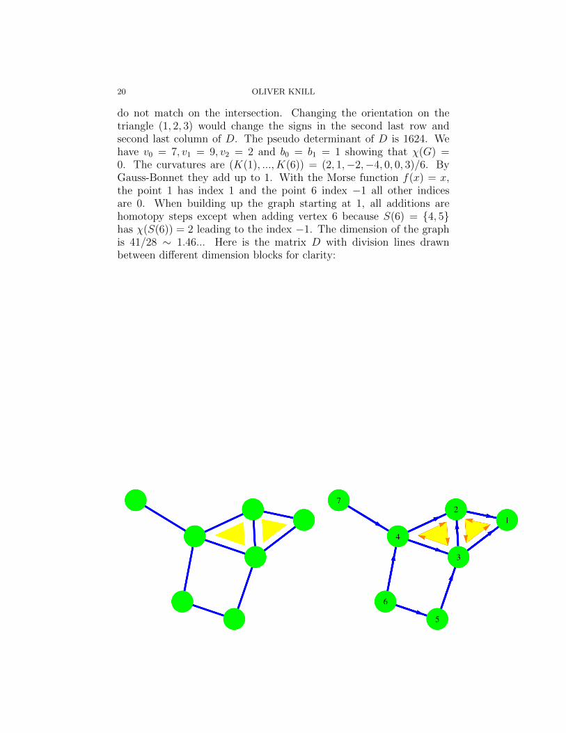
The figure shows at a graph with 7 vertices and 9 edges homotopic toC4. Since G has 2 triangles, the Euler characteristic is 0. The secondpicture shows it with the orientation used to generate the matrix D.The two triangles do not form a surface because their orientations

20 OLIVER KNILL

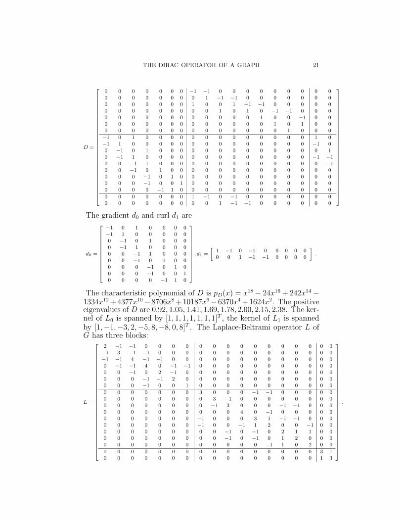
do not match on the intersection. Changing the orientation on thetriangle (1, 2, 3) would change the signs in the second last row andsecond last column of D. The pseudo determinant of D is 1624. Wehave v0 = 7, v1 = 9, v2 = 2 and b0 = b1 = 1 showing that χ(G) =0. The curvatures are (K(1), ..., K(6)) = (2, 1,−2,−4, 0, 0, 3)/6. ByGauss-Bonnet they add up to 1. With the Morse function f(x) = x,the point 1 has index 1 and the point 6 index −1 all other indicesare 0. When building up the graph starting at 1, all additions arehomotopy steps except when adding vertex 6 because S(6) = 4, 5has χ(S(6)) = 2 leading to the index −1. The dimension of the graphis 41/28 ∼ 1.46... Here is the matrix D with division lines drawnbetween different dimension blocks for clarity:


D =

0 0 0 0 0 0 0 −1 −1 0 0 0 0 0 0 0 0 0

0 0 0 0 0 0 0 0 1 −1 −1 0 0 0 0 0 0 0

0 0 0 0 0 0 0 1 0 0 1 −1 −1 0 0 0 0 00 0 0 0 0 0 0 0 0 1 0 1 0 −1 −1 0 0 0

0 0 0 0 0 0 0 0 0 0 0 0 1 0 0 −1 0 0

0 0 0 0 0 0 0 0 0 0 0 0 0 1 0 1 0 00 0 0 0 0 0 0 0 0 0 0 0 0 0 1 0 0 0

−1 0 1 0 0 0 0 0 0 0 0 0 0 0 0 0 1 0

−1 1 0 0 0 0 0 0 0 0 0 0 0 0 0 0 −1 0

0 −1 0 1 0 0 0 0 0 0 0 0 0 0 0 0 0 10 −1 1 0 0 0 0 0 0 0 0 0 0 0 0 0 −1 −10 0 −1 1 0 0 0 0 0 0 0 0 0 0 0 0 0 −10 0 −1 0 1 0 0 0 0 0 0 0 0 0 0 0 0 00 0 0 −1 0 1 0 0 0 0 0 0 0 0 0 0 0 0

0 0 0 −1 0 0 1 0 0 0 0 0 0 0 0 0 0 0

0 0 0 0 −1 1 0 0 0 0 0 0 0 0 0 0 0 0

0 0 0 0 0 0 0 1 −1 0 −1 0 0 0 0 0 0 00 0 0 0 0 0 0 0 0 1 −1 −1 0 0 0 0 0 0

The gradient d0 and curl d1 are

d0 =

−1 0 1 0 0 0 0

−1 1 0 0 0 0 00 −1 0 1 0 0 0

0 −1 1 0 0 0 0

0 0 −1 1 0 0 00 0 −1 0 1 0 0

0 0 0 −1 0 1 0

0 0 0 −1 0 0 10 0 0 0 −1 1 0

, d1 =

[1 −1 0 −1 0 0 0 0 0

0 0 1 −1 −1 0 0 0 0

].

The characteristic polynomial of D is pD(x) = x18 − 24x16 + 242x14 −1334x12 + 4377x10− 8706x8 + 10187x6− 6370x4 + 1624x2. The positiveeigenvalues of D are 0.92, 1.05, 1.41, 1.69, 1.78, 2.00, 2.15, 2.38. The ker-nel of L0 is spanned by [1, 1, 1, 1, 1, 1, 1]T , the kernel of L1 is spannedby [1,−1,−3, 2,−5, 8,−8, 0, 8]T . The Laplace-Beltrami operator L ofG has three blocks:

L =

2 −1 −1 0 0 0 0 0 0 0 0 0 0 0 0 0 0 0−1 3 −1 −1 0 0 0 0 0 0 0 0 0 0 0 0 0 0

−1 −1 4 −1 −1 0 0 0 0 0 0 0 0 0 0 0 0 00 −1 −1 4 0 −1 −1 0 0 0 0 0 0 0 0 0 0 0

0 0 −1 0 2 −1 0 0 0 0 0 0 0 0 0 0 0 0

0 0 0 −1 −1 2 0 0 0 0 0 0 0 0 0 0 0 00 0 0 −1 0 0 1 0 0 0 0 0 0 0 0 0 0 0

0 0 0 0 0 0 0 3 0 0 0 −1 −1 0 0 0 0 0

0 0 0 0 0 0 0 0 3 −1 0 0 0 0 0 0 0 0

0 0 0 0 0 0 0 0 −1 3 0 0 0 −1 −1 0 0 00 0 0 0 0 0 0 0 0 0 4 0 −1 0 0 0 0 0

0 0 0 0 0 0 0 −1 0 0 0 3 1 −1 −1 0 0 0

0 0 0 0 0 0 0 −1 0 0 −1 1 2 0 0 −1 0 00 0 0 0 0 0 0 0 0 −1 0 −1 0 2 1 1 0 0

0 0 0 0 0 0 0 0 0 −1 0 −1 0 1 2 0 0 00 0 0 0 0 0 0 0 0 0 0 0 −1 1 0 2 0 0

0 0 0 0 0 0 0 0 0 0 0 0 0 0 0 0 3 10 0 0 0 0 0 0 0 0 0 0 0 0 0 0 0 1 3

.

22 OLIVER KNILL

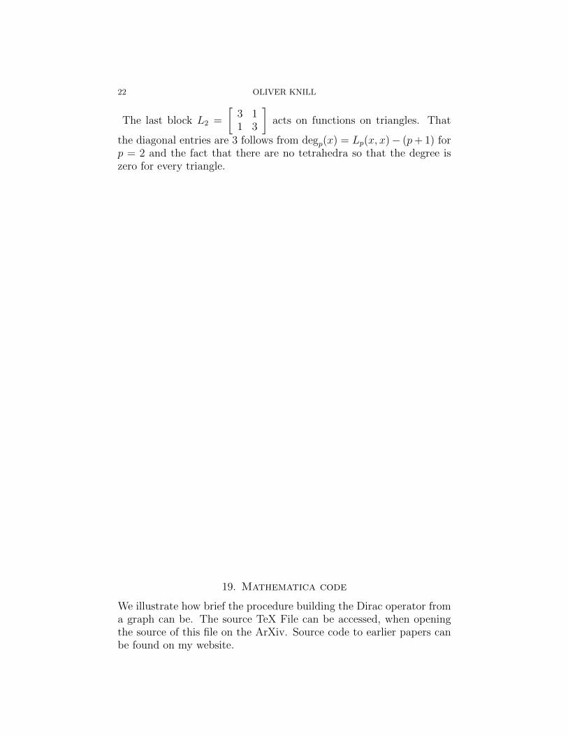
The last block L2 =

[3 11 3

]acts on functions on triangles. That

the diagonal entries are 3 follows from degp(x) = Lp(x, x)− (p+ 1) forp = 2 and the fact that there are no tetrahedra so that the degree iszero for every triangle.

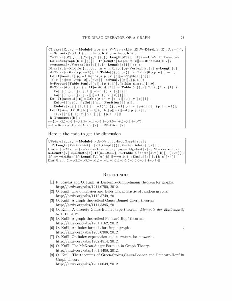
19. Mathematica code

We illustrate how brief the procedure building the Dirac operator froma graph can be. The source TeX File can be accessed, when openingthe source of this file on the ArXiv. Source code to earlier papers canbe found on my website.


Cl iques [ K , k ] :=Module [n , u ,m, s ,V=VertexLi s t [K] ,W=EdgeList [K] ,U, r= ,s=Subsets [V, k , k ] ; n=Length [V ] ; m=Length [W] ;

Y=Table [W[ [ j , 1 ] ] ,W[ [ j , 2 ] ] , j ,Length [W] ] ; I f [ k==1,r=V, I f [ k==2,r=Y,Do[ u=Subgraph [K, s [ [ j ] ] ] ; I f [Length [ EdgeList [ u]]==Binomial [ k , 2 ] ,r=Append [ r , Ver texLi s t [ u ] ] ] , j ,Length [ s ] ] ] ] ; r ] ;

Dirac [ s ] :=Module [ a , b , q , l , n , v ,m,R, t , d , q=VertexL i s t [ s ] ; n=Length [ q ] ;

d=Table [0 ,p , n−1 ] ; l=Table [ ,p , n ] ; v=Table [ 0 ,p , n ] ; m=n ;Do[ I f [m==n , l [ [ p ] ]= Cl iques [ s , p ] ; v [ [ p ] ]=Length [ l [ [ p ] ] ] ;I f [ v [ [ p ]]==0 ,m=p−2 ] ] ,p , n ] ; t=Sum[ v [ [ p ] ] , p , n ] ;b=Prepend [Table [Sum[ v [ [ p ] ] , p , 1 , k ] , k ,Min [ n ,m+1 ] ] , 0 ] ;R=Table [ 0 , t , t ] ; I f [m>0, d [ [ 1 ] ] = Table [ 0 , j , v [ [ 2 ] ] , i , v [ [ 1 ] ] ] ;

Do[ d [ [ 1 , j , l [ [ 2 , j , 1 ] ] ] ]= −1 , j , v [ [ 2 ] ] ] ;Do[ d [ [ 1 , j , l [ [ 2 , j , 2 ] ] ] ] = 1 , j , v [ [ 2 ] ] ] ] ;

Do[ I f [m>=p , d [ [ p ] ]=Table [ 0 , j , v [ [ p+1] ] , i , v [ [ p ] ] ] ;Do[ a=l [ [ p+1, i ] ] ;Do[ d [ [ p , i , Position [ l [ [ p ] ] ,Delete [ a , j ] ] [ [ 1 , 1 ] ] ] ] = ( − 1 ) ˆ j , j , p+1 ] , i , v [ [ p+1 ] ] ] ] , p , 2 , n−1 ] ;

Do[ I f [m>=p ,Do[R [ [ b [ [ p+1]]+ j , b [ [ p ] ]+ i ] ]=d [ [ p , j , i ] ] , i , v [ [ p ] ] , j , v [ [ p+1 ] ] ] ] , p , n−1 ] ;

R+Transpose [R ] ] ;s=1−>2,2−>3,3−>1,3−>4,4−>2,3−>5,5−>6,6−>4,4−>7;s=UndirectedGraph [ Graph [ s ] ] ; DD=Dirac [ s ] Here is the code to get the dimensionUSphere [ s , a ] :=Module [ , b=NeighborhoodGraph [ s , a ] ;I f [Length [ Ver texLi s t [ b ] ]<2 ,Graph [ ] , VertexDelete [ b , a ] ] ] ;

Dim [ s ] :=Module [ v=VertexLi s t [ s ] , u , n ,m, e=EdgeList [ s ] , VL=VertexLi s t ;n=Length [ v ] ;m=Length [ e ] ; I f [ n==0,u= ,u=Table [ USphere [ s , v [ [ k ] ] ] , k , n ] ] ;I f [m==0,0,Sum[ I f [Length [VL[ u [ [ k ] ] ] ]==0 ,0 ,1 ]+Dim [ u [ [ k ] ] ] , k , n ] / n ] ] ;

Dim [ Graph[1−>2,2−>3,3−>1,3−>4,4−>2,3−>5,5−>6,6−>4,4−>7]] References

[1] F. Josellis and O. Knill. A Lusternik-Schnirelmann theorem for graphs.http://arxiv.org/abs/1211.0750, 2012.

[2] O. Knill. The dimension and Euler characteristic of random graphs.http://arxiv.org/abs/1112.5749, 2011.

[3] O. Knill. A graph theoretical Gauss-Bonnet-Chern theorem.http://arxiv.org/abs/1111.5395, 2011.

[4] O. Knill. A discrete Gauss-Bonnet type theorem. Elemente der Mathematik,67:1–17, 2012.

[5] O. Knill. A graph theoretical Poincare-Hopf theorem.http://arxiv.org/abs/1201.1162, 2012.

[6] O. Knill. An index formula for simple graphs .http://arxiv.org/abs/1205.0306, 2012.

[7] O. Knill. On index expectation and curvature for networks.http://arxiv.org/abs/1202.4514, 2012.

[8] O. Knill. The McKean-Singer Formula in Graph Theory.http://arxiv.org/abs/1301.1408, 2012.

[9] O. Knill. The theorems of Green-Stokes,Gauss-Bonnet and Poincare-Hopf inGraph Theory.http://arxiv.org/abs/1201.6049, 2012.

24 OLIVER KNILL

[10] O. Knill. A Brouwer fixed point theorem for graph endomorphisms. Fixed PointTheory and Applications, 85, 2013.

[11] O. Knill. Cauchy-Binet for pseudo determinants.http://arxiv.org/abs/1306.0062, 2013.

[12] O. Knill. An integrable evolution equation in geometry.http://arxiv.org/abs/1306.0060, 2013.

Department of Mathematics, Harvard University, Cambridge, MA, 02138

introduction dirac operator v - harvard department of …knill/seminars/providence/ilas.pdfthe dirac...

Documents