arX

iv:1

206.

4090

v1 [

astr

o-ph

.GA

] 1

8 Ju

n 20

12

Interstellar extinction and interstellar polarization: old

and new models

N.V. Voshchinnikov

Sobolev Astronomical Institute, St. Petersburg University, Universitetskii prosp., 28,

St. Petersburg, 198504 Russia

Abstract

The review contains an analysis of the observed and model curves of theinterstellar extinction and polarization. The observations mainly give in-formation on dust in diffuse and translucent interstellar clouds. The fea-tures of various dust grain models including spherical/non-spherical, homo-geneous/inhomogeneous particles are discussed. A special attention is de-voted to the analysis of the grain size distributions, alignment mechanismsand magnetic field structure in interstellar clouds. It is concluded that theinterpretation of interstellar extinction and polarization is not yet complete.

Keywords: Light scattering, Nonspherical particles, Composite particles,Extinction, Polarization, Magnetic field

1. Introduction

The properties of cosmic dust grains in various objects from comets todistant galaxies are derived from observations of interstellar extinction, in-terstellar polarization, scattered radiation, infrared (IR) continuum emissionand IR features. Modelling of these observations is aimed at estimates ofthe grain size, chemical composition, shape, structure, and alignment. Theobserved wavelength dependencies of interstellar extinction and polarization(interstellar extinction A(λ) and polarization P (λ) curves) still remain themain sources of information on dust in diffuse and translucent interstellarclouds.

Email address: nvv@astro.spbu.ru (N.V. Voshchinnikov)

Preprint submitted to JQSRT November 3, 2018

In this review, we discuss observations and modelling of the interstellarextinction and polarization curves. Special attention is paid to various dustgrain models. For an extended consideration of the properties of dust indifferent astronomical objects see [1, 2, 3, 4, 5]. Excellent historical reviewson dust astrophysics are given by Dorschner [6] and Li [7].

2. Extinction

2.1. Extinction curve: production and fitting

The normalized extinction curves A(n)(λ−1) commonly studied can becalculated as the ratio of the colour excess of a star behind the dusty cloudE(λ− V ) to the colour excess E(B − V )

A(n)(λ−1) ≡E(λ− V )

E(B − V )=A(λ) − AV

AB − AV

. (1)

Here, AB and AV is the extinction in the B and V bands, respectively. Some-times, the normalization of the extinction curve on AV or extinction in an-other band is used.

In such a manner we can determine only the “selective” extinction (red-dening), i.e. the difference of extinction at two wavelengths. The absolutevalue of extinction can be found as

AV = RVE(B − V ), (2)

where the coefficient RV is often evaluated from observations in the visibleand IR taking into account that Aλ → 0 when λ → ∞. From Eq. (1), itfollows that

RV =AV

E(B − V )= −

E(∞− V )

E(B − V ). (3)

In the diffuse medium on average RV = 2.4 − 3.6 [8].In general, the interstellar extinction curve has a power law-like rise from

the IR to the visible, a prominent feature (bump) near λ 2175 A, and a steeprise in the far-UV. This rise is a manifestation of the very strong featurewith a maximum near λ ≈ 700 A [9]. Figure 1 shows the extinction curveaveraged over 243 Galactic B and late–O stars [8]. In the near IR-visible partof the spectrum, the distinction between the extinction curves of differentstars is rather small. The IR extinction at wavelengths λ = 0.7–5µm wasapproximated by the power-law dependence: A(λ) ∝ λ−β with β = −1.84

2

0 2 4 6 8 10

λ−1, µm-1

-5

0

5

10

E(λ

-V)/

E(B

-V)

Average curve, RV=3.00, c4=0.32, c5=6.10

HD 147933, RV=4.41, c4=0.27, c5=6.06

HD 148579, RV=4.01, c4=0.38, c5=6.05

HD 147701, RV=4.03, c4=0.58, c5=5.97

Oph-Sco

0 2 4 6 8 10

λ−1, µm-1

-5

0

5

10

E(λ

-V)/

E(B

-V)

Average curve, RV=3.00, c4=0.32, c5=6.10

HD 147165, RV=3.60, c4=0.41, c5=7.50

HD 144470, RV=3.71, c4=0.47, c5=7.36

HD 148579, RV=4.01, c4=0.38, c5=6.05

Oph-Sco

Figure 1: The average extinction curve for 243 Galactic stars with 2.4 < RV < 3.6 and theextinction curves in the direction of six stars in Sco-Oph [8]. The values of the coefficientRV and the UV fitting coefficients c4 and c5 (Eq. (4)) are indicated in the legend. Theeffect of variations of coefficients c4 (left panel) and c5 (right panel) is illustrated. Adaptedfrom [8].

[10]. Fitzpatrick and Massa [11] found that the index β was RV -dependent:β > 2 ifRV < 3 and β < 1.5 ifRV > 3. The mid-IR extinction at wavelengthsλ >∼ 3µm measured in the Galactic plane [12] and toward the Galactic centre[13] becomes grayer than the near-IR extinction.

In the UV region, the extinction curves differ strongly [8, 14, 15] (see alsoFig. 1) demonstrating that the mean curve in the UV obviously has littlemeaning. The position of the UV bump center varies a little from star tostar and occurs at λ0 = 2174 ± 17 A or λ−1

0 = 4.599 ± 0.012µm−1. Thetotal half-width of the bump is W = 0.992± 0.058µm−1 that corresponds to470 ± 27 A [16].

Dorschner [17] was the first who suggested to approximate the shapeof the bump profile by the classical (Lorentzian) dispersion profile. Afterexamination of the IUE extinction curves for many lines of sight, Fitzpatrickand Massa [8, 16, 18] deduced a single analytical expression with a smallnumber of parameters describing extinction in the region 1150 A ≤ λ <

3

2700 A (x ≡ λ−1)

A(n)(x) =E(λ− V )

E(B − V )=

c1 + c2x + c3D(x,W, x0), x ≤ c5,c1 + c2x + c3D(x,W, x0) + c4(x− c5)

2, x > c5,(4)

where

D(x,W, x0) =x2

(x2 − x20)2 + x2W 2

. (5)

Originally, the value of c5 was fixed at 5.9µm−1 [18]. Equation (4) consists of:i) a Lorentzian-like bump term (requiring three parameters, correspondingto the bump width W , position x0, and strength c3), ii) a far-UV curvatureterm (two parameters c4 and c5; see Fig. 1 for illustration), and iii) a linearterm underlying the bump and the far-UV (two parameters c1 and c2). Theparameters of the average extinction curve presented in Fig. 1 are: RV =3.001, x0 = 4.592µm−1, W = 0.922µm−1, c1 = −0.175, c2 = 0.807, c3 =2.991, c4 = 0.319, c5 = 6.097 [8].

Fitzpatrick and Massa [8] note that there is no correlation between theUV and IR portions of the Galactic extinction curves. This fact is illustratedby Fig. 2 where the dependence of the coefficient RV on the quantity describ-ing the strength of the far-UV extinction curvature ∆1250 = c4(8.0 − c5)

2 isshown. Absence of the correlation between RV and ∆1250 contradicts theoften used representation of the extinction curves from the UV to IR as aone-parameter family dependent on RV (so called CCM model introducedby Cardelli, Clayton and Mathis [19, 20]). As mentioned in [8], the relationsbetween RV and UV extinction found in [19, 20] can arise from sample selec-tion and methodology. Evidently, some bias relates to the number of cloudsavailable in the line of sight, i.e. to the distance to the star. There exists awide scatter of the data for nearby stars in comparison with the distant stars(see Fig. 2). A large difference in extinction for the nearby stars observedthrough single clouds was first noted by Kre lowski and Wegner [21]. It shouldbe mentioned that the major part of anomalous or peculiar extinction sight-lines studied so far are related to not very distant stars [22, 23, 24, 25, 26].

2.2. Interpretation: homogeneous spheres

The extinction of stellar radiation at the wavelength λ after passing adust cloud is equal to

A(λ) = −2.5 log I(λ)/I0(λ) ≈ 1.086τ(λ), (6)

4

0 2 4 6

2

3

4

5

6

7

RV

Data from Fitzpatrick & Massa (2007)Stars with D ≤1kpc (120)Stars with D>1kpc (201)Mean curve

∆1250Figure 2: The coefficient RV in dependence on the quantity ∆1250 = c4(8.0−c5)

2 showingthe strength of the far-UV extinction curvature in the direction of 321 stars with knowndistances from [8]. Filled and open circles show data for stars with the distancesD ≤ 1 kpcand D > 1 kpc, respectively. Cross corresponds to the average Galactic extinction curve.

where I0(λ) is the source (star) intensity, τ(λ) the optical thickness whichcan be found as the total extinction cross-section of all particles types alongthe line of sight in a given direction. Interpretation of the interstellar ex-tinction is often performed using homogeneous spherical particles of varioussize distributions. Then, the wavelength dependence of extinction can becalculated as

A(λ) = 1.086∑

j

∫ D

0

rs,max,j∫

rs,min,j

Cext,j(m, rs, λ)nj(rs) drs,j dl. (7)

Here, nj(rs) is the size distribution of spherical dust grains of the typej and radius rs with the lower cut-off rs,min and the upper cut-off rs,max,Cext(...) = πr2s Qext(...) the extinction cross-section, Qext the extinction effi-

5

ciency factor, m the refractive index, D the distance to a star. From Eq. (7),an important conclusion follows: the wavelength dependence of interstellarextinction is completely determined by the wavelength dependence of theextinction efficiency Qext.

0

1

2

3

4

5Qext

rs=0.005µm

rs=0.01µm

rs=0.02µm

rs=0.05µm

rs=0.1µm

rs=0.3µm

astrosil

λ-1.33

0 2 4 6 8 10

λ-1, µm-1

0

1

2

3

4

5Qext

amorphous carbon (AC1)

λ-1.33

Figure 3: Wavelength dependence of the extinction efficiency factors for homogeneousspherical particles of different sizes consisting of astronomical silicate and amorphous car-bon. The dashed segment shows the approximate wavelength dependence of the meanGalactic extinction curve at optical wavelengths. Adapted from [2].

The average interstellar extinction curve in the visible-near UV can beapproximated by the power law A(λ) ∝ λ−1.3 [8]. Such wavelength depen-dence can be produced by submicron-sized particles of the typical radius〈r〉 ≈ 0.05 − 0.1µm. In this case, for more absorbing materials like amor-phous carbon or iron we have smaller particles and for less absorbing ma-terials like silicate or ice we need larger particles (see Fig. 3). So, from the

6

wavelength dependence of extinction only the product of the typical particlesize and the refractive index 〈r〉 |m − 1| ≈ const. can be determined, butnot the size or chemical composition of dust grains separately. In order tosolve this problem, the dust-phase abundances of the main elements formingdust (C, O, Mg, Si and Fe) need to be taken into account and to reproducethe absolute extinction. Unfortunately, despite numerous observations of theinterstellar absorption lines (see a compilation of Gudennavar et al. [27])abundances with good accuracy are known just for a restricted number ofdiffuse and translucent clouds [28, 29, 30].

Another problem having many solutions is identification of the UV bumpnear λ 2175 A. Various materials with isotropic and anisotropic propertiessuch as silicate (enstatite), irradiated quartz, oxides (MgO, CaO), organicmolecules have been considered as carrier candidates (see discussion in [1, 2]).However, the position and width of the bump are strongly suggestive ofπ → π∗ transitions in graphitic or aromatic carbonaceous species domi-nating by sp2 bonding. Therefore, small graphite particles and polycyclicaromatic hydrocarbons (PAH molecules) are considered as the favourite ma-terials [31, 32, 33]. Unfortunately, the reliable identification of the carrierremains unknown. The attempts to find the UV or visual bands of PAHshave failed [34, 35]. We cannot even determine the size of graphite spheresresponsible for the λ 2175 A feature (see Fig. 4). The profiles with the centralposition near λ−1

0 = 4.6µm−1 can be obtained if we take particles with theradius rs ≈ 0.015µm (Fig. 4, left panel). Although for single-size particlesthe width of the calculated profiles is smaller than the observed one, a simplebi-modal size distribution allows a fit to both the position and the width ofthe mean Galactic profile (Fig. 4, right panel).

The far-UV extinction can be explained by tiny particles of the typicalradius 〈r〉 ≈ 0.01 − 0.03 µm (see Fig. 3). The number density of such grainsis ∼ 1000 times large than the submicron particles producing the visual-near-IR extinction [36]. Because of temperature fluctuations, such particlesare protected from growth by accretion in the interstellar clouds. The far-UV rise of extinction may be also fitted as the low-energy side of σ → σ∗

transitions in PAHs (see [37] for discussion).By using particles of different chemical composition and applying Eq. (7)

it is possible to interpret the interstellar extinction and to reconstruct thedust size distribution. In the pioneer work of Oort and van de Hulst [38]the size distribution of icy grains was found in the tabular form. Later,Greenberg [39] fitted it with an exponential function. By using minimiza-

7

3.5 4.0 4.5 5.0 5.5 6.0

λ-1, µm-1

0.4

0.6

0.8

1.0

1.2

rs=0.005µm

rs=0.010µm

rs=0.015µm

rs=0.020µm

rs=0.030µm

observations

Qex

t/Qex

t(λ21

75)

graphite, 2/3-1/3

3.5 4.0 4.5 5.0 5.5 6.0

λ-1, µm-1

0.4

0.6

0.8

1.0

1.2

1/2[Qext

(0.005µm)+Qext

(0.03µm)]

observations

Qex

t/Qex

t(λ21

75)

graphite, 2/3-1/3

Figure 4: Normalized extinction efficiencies for graphite spheres. The curve marked as“observations” corresponds to the wavelength dependence of the UV bump given by themean Galactic extinction curve. The central position of the observed UV bump and itsrange of variations are marked. The left panel shows extinction of single size graphitespheres. The right panel shows the summary extinction of two graphite spheres withradii rs = 0.005µm and rs = 0.03µm (from left panel) taken in equal proportions. Allcalculations were made in the “2/3–1/3” approximation for the averaged extinction factorsQext = 2/3Qext(ε⊥) + 1/3Qext(ε||), where ε⊥ and ε|| are the dielectric functions for twocases of orientation of the electric field relative to the basal plane of graphite. Adaptedfrom [2].

tion of the χ2 statistic, Mathis et al. [41] reconstructed the power-law sizedistribution for silicate and graphite particles. These two simplest size distri-butions contain the only parameter (except for the lower and upper cut-offs,see Table 1). More complicated two-parameter distributions were applied byWickramasinghe and Guillaume [42] and Wickramasinghe and Nandy [43] inorder to fit the mean extinction curve with graphite grains and a mixture ofgraphite, iron and silicate grains, respectively. A comprehensive discussionof the early attempts to model the interstellar extinction can be found in thereview of Wickramasinghe and Nandy [44].

The size distributions of dust grains can be also found from extinctionmeasurements by solving the inverse problem. It has been made by themaximum entropy method [45] and by Tikhonov’s method of regulariza-tion [47, 48, 49]. The obtained size distributions were approximated byrather complicated functions containing up to 14 parameters (see Table 1).Complexity of the size distributions used in [31, 47] is explained by the chal-lenge in reproducing the diffuse Galactic IR emission as well.

8

Table 1: Dust size distributions used for interpretation of interstellar extinction.

Author(s) (year) reference; size distribution function Nparameters

Greenberg (1968) [39]; exponential

n(rs) ∝ exp[

−5 (rs/rs0)3] 1

Isobe (1973) [40]; exponentialn(rs) ∝ exp [− (rs/rs0)] 1

Mathis et al. (1977) [41]; power-law; MRN mixturen(rs) ∝ r−q

s 1

Wickramasinghe and Guillaume (1965) [42]; normal

n(rs) ∝ exp[

− (rs − rs)2 /(2σ2)

]

2

Wickramasinghe and Nandy (1971) [43]; lognormal

n(rs) ∝ rr1s exp[

−1/2 (rs/r2)3] 2

Kim et al. (1994) [45]; power-law with exponential decayn(rs) ∝ r−γ

s exp(−rs/rsb) 2

Mathis (1996) [46]; power-law with exponential decayn(rs) ∝ r−γ0

s exp[−(γ1rs + γ2/rs + γ3/r2s )] 4

Weingartner and Draine (2001) [31]; two lognormal

n(rs) ∝ DC(rs) +CC, Si

rs

(

rsrt; C, Si

)αC, Si

×

1 + βC, Sirs/rt; C, Si, β ≥ 0(1 − βC,Sirs/rt; C,Si)

−1, β < 0

×

1, 3.5 A < rs < rt; C, Si

exp−[(rs − rt; C, Si)/rt; C,Si]3, rs > rt; C,Si

11

Zubko et al. (2004) [47];log n(rs) = c0 + b0 log(rs) − b1| log(rs/a1)|

m1

−b2| log(rs/a2)|m2 − b3|rs − a3|

m3 − b4|rs − a4|m4 14

9

2.3. Interpretation: inhomogeneous and composite particles

Progress in observations, the light scattering and grain growth theoriesgave rise to new dust models with grains more complicated than homogeneousspheres.

Wickramasinghe [50, 51] was the first who studied the optical propertiesof core-mantle grains which could grow in interstellar clouds due to accre-tion of volatile elements on refractory particles. He calculated extinctionproduced by graphite core–ice mantle and silicate core–ice mantle spheres.Extensive calculations of extinction for graphite core–ice mantle particleswere also made by Greenberg [39] who later proposed the existence of parti-cles with silicate cores coated by a layer of organic material in diffuse cloudsand silicate-organic-ice grains in molecular clouds [36]. Such grains were acomponent of the dust mixture reproducing interstellar extinction [52].

The growth of interstellar grains due to their coagulation in dense molec-ular cloud cores may result in formation of grain aggregates with large voids[53]. The internal structure of such composite grains can be very compli-cated, and their optical properties cannot be described by the model of core–mantle spheres. Exact calculations are possible for complex aggregates ofrather small sizes [54, 55, 56]. Therefore, very complicated particles are re-placed by more simple “optically equivalent” ones. A very popular approachis to make calculations using the Mie theory for homogeneous spheres with anaverage refractive index derived from one of the mixing rules of the effectivemedium theory (EMT; see, e.g., [46, 47, 57] and Table 2). Another possibil-ity to treat composite aggregate grains is to consider multi-layered particles.As shown by Voshchinnikov and Mathis [60] for spheres and by Farafonovand Voshchinnikov [63] for spheroids, the scattering characteristics of layeredparticles slightly depend on the order of materials and become close to some“average” ones, when the number of layers exceeds 15 − 20. According toestimates made in [64], the optical properties of layered particles resemblethose of heterogeneous particles having inclusions of various sizes while theEMT-Mie approach can be used if the particles have small (in comparisonwith the wavelength of the incident radiation) “Rayleigh” inclusions.

Inhomogeneous and composite particles have an advantage over homo-geneous ones as there exists the possibility of including vacuum as one ofthe materials. The new dust models with fluffy, porous particles are able toproduce the same extinction with a smaller amount of solid material thandust models with compact particles. The amount of vacuum in a particle

10

Table 2: Models of inhomogeneous spherical grains used for interpretation of interstellarextinction.

Author(s) (year) reference Model

Wickramasinghe (1963) [50]; graphite core–ice mantleGreenberg (1968) [39]

Wickramasinghe (1970)[51] silicate core–ice mantle

Greenberg, Li (1996) [52] silicate core–organic mantle

Mathis and Whiffen (1989) [57]; EMT-Mie: silicate + amorphousMathis (1996) [46] carbon + iron + voids

Zubko et al. (1998, 2004) [47, 49] EMT-Mie: silicate + organicrefractory + water ice + voids

Vaidya et al. (2001) [58] silicates with graphite inclusions

Voshchinnikov and Mathis (1999) [60]; multi-layered: vacuum/silicate/Voshchinnikov et al. (2006) [61] amorpous carbon

Iatı et al. (2008) [62]; four-layered: vacuum–Cecchi-Pestellini et al. (2010) [37]; silicate–sp2-carbon–Zonca et al. (2011) [24] sp3-carbon

Rai and Rastogi (2012) [26] nanodiamonds coated byamorpous carbon or graphite

can be characterized by its porosity P (0 ≤ P < 1)

P = Vvac/Vtotal = 1 − Vsolid/Vtotal. (8)

The role of porosity in extinction is seen from Fig. 5 that gives the wavelengthdependence of the normalized cross section

C(n)ext =

Cext(porous grain)

Cext(compact grain of same mass)=

(1 − P)−2/3 Qext(porous grain)

Qext(compact grain of same mass). (9)

This quantity shows how porosity influences the extinction cross section. Asfollows from Fig. 5, as P increases the model predicts a growth of extinctionof porous particles in the far-UV and a decrease in the visual–near-UV. In

11

0 1 2 3 4 5 6 7 8 9 10

0

1

2

3

λ-1, µm-1

extC(n) layered sphere, r

s=0.1µm

=0.0

=0.1

=0.3

=0.5

=0.7

=0.9

Figure 5: Wavelength dependence of the normalized extinction cross section (see Eq. (9))for multi-layered spherical particles with rs, compact = 0.1µm. The particles are of the

same mass but of different porosity. If C(n)ext > 1, extinction of a porous particle is larger

than that of a compact one of the same mass. Adapted from [61].

comparison with compact grains, layered particles can also produce ratherlarge extinction in the near-IR. This is especially important for the expla-nation of the flat extinction across the 3 − 8µm wavelength range measuredfor several lines of sight (see [13, 61] for discussion). It is also seen fromFig. 5 that an addition of vacuum into particles does not lead to a growthof extinction at all wavelengths and material saving1. Evidently, the finalconclusion can be made after detailed comparison of the observations withtheoretical calculations at many wavelengths.

Table 2 contains information about models of inhomogeneous sphericalgrains used for the interpretation of interstellar extinction. Inhomogeneousnon-spherical particles of the simplest shapes (cylinders, spheroids) are alsoused for simultaneous interpretation of interstellar extinction and polariza-tion (see Table 4). In this case major attention has been paid to the modelling

1This supports a conclusion of Li [65] that an interpretation of the observed interstellarextinction curve using only very porous grains should not give any gain in dust-phaseabundances.

12

of polarization because extinction usually has only a slight dependence onthe particle shape and orientation [2, 66].

The models discussed in this Section were first applied to interpretat-ing the average Galactic extinction curve. Modelling of extinction in severalsightlines has been also performed [22, 23, 26, 31, 48, 49, 61, 67, 68, 69, 70].The models include multi-component mixtures of bare particles with a rathercomplicated size distribution function or/and inhomogeneous particles andPAHs and often took into account abundance restrictions. Especially popu-lar is the direction to the halo star HD 210121 with very high UV extinction.The extinction for this star has been modeled by Li and Greenberg [69] witha mixture of silicate core–organic mantle spheres, bare spheres and PAHs, byLarson et al. [70] and by Clayton et al. [71] with two-component (silicate,graphite) and three-component (silicate, graphite, amorphous carbon) mod-els, by Weingartner and Draine [31] who considered the mixture of carbona-ceous and silicate grains with the size distribution given in Table 1, and byRai and Rastogi [26] who used a silicate-graphite mixture and nanodiamondscoated by carbon. This list illustrates the non-uniquiness of parameters ofdust grains obtained from modelling.

A similar conclusion about the ambiguity of the modelling follows fromseveral attempts to interpret the peculiar extinction curves characterized bya broad λ 2175 A bump and a steep far-UV rise or a sharp λ 2175 A bumpand flat far-UV extinction (see Fig. 1). Using the model of Weingartner andDraine [31] (see Table 1), Mazzei and Barbaro [23] derived the parameters ofthe size distribution for 64 stars. Variations of the parameters were attributedto the selective grain destruction in both shocks and grain-grain collisions.Zonca et al. [24] found an excellent fit for different extinction curves for15 sightlines with the mixture of layered porous grains for reproduction ofthe near-IR-visual extinction and PAHs to account for the bump and far-UVextinction. Large grains consisting of silicates coated by layers from graphiticand polymeric amorphous carbons (see Table 2) were suggested in the modelof Jones et al. [72] (see [73] for more details). Rai and Rastogi [26] analyzedanomalous extinction curves in the direction of 10 stars and showed that avery good match with the far-UV rise of extinction was obtained if to includenanodiamonds coated by graphite or amorphous carbon as a component ofthe silicate-graphite mixture.

Summarizing this discussion of the interstellar extinction, it should benoted that there is a wide diversity in the models and the non-uniqueness inthe results. In spite of numerous attempts to use very complicated inhomo-

13

geneous particles, the Mie theory for homogeneous spheres keeps its leadingposition as a main tool for the interpretation of interstellar extinction. Fur-ther progress in the investigations should include a clear role for PAHs andmodelling of the extinction on the basis of interstellar abundances in selecteddirections. A sofisticated undertstanding of the origin of UV extinction, theavailable solid-state material and the grain growth process would stimilategoing from simple Mie theory to justified models of complex particles.

3. Polarization

3.1. Observations: Serkowski curve and polarizing efficiency

Interstellar linear polarization is caused by the linear dichroism of the in-terstellar medium due to the presence of non-spherical aligned grains. Dustgrains must have sizes close to the wavelength of the incident radiation andspecific magnetic properties to efficiently interact with the interstellar mag-netic field. The direction of alignment must not coincide with the line of sightand there must be no cancellation of polarization during the propagation ofradiation through the interstellar medium.

Interstellar polarization was discovered in 1949 by Hiltner [74], Hall [75]and Dombrovskii [76] in the course of the search for the Sobolev-Chandrase-khar effect2. The wavelength dependence of polarization P (λ) in the vis-ible part of spectrum is described by an empirical formula suggested bySerkowski [77]

P (λ)/Pmax = exp[−K ln2(λmax/λ)]. (10)

This formula has three parameters: the maximum degree of polarizationPmax, the wavelength corresponding to it λmax and the coefficient K char-acterizing the width of the Serkowski curve. Initially, the coefficient K waschosen by Serkowski [77, 78] to be equal to 1.15(3).

2Sobolev and Chandrasekhar have shown that the polarization of radiation at the limbof a star due to the electronic (Thomson) scattering should reach∼ 12%. Eclipsing binarieswith extended atmospheres have been suggested in order to observe the effect.

3The Serkowski curve is just one of possible approximations of the observed dependenceP (λ). For example, Wolstencroft and Smith [79] have suggested the representation

P (λ)/Pmax = 2K(λ/λmax + λmax/λ)−K.

When K = 2.25 this curve lies within 1% of the Serkowski curve with K = 1.15 in thewavelength interval 0.22− 1.40 µm.

14

The values of Pmax in the diffuse interstellar medium usually do not exceed10%. The ratios Pmax/E(B − V ) and Pmax/AV determine the polarizingefficiency of the interstellar medium in a selected direction. There existempirically found upper limits on these ratios [78]

Pmax/E(B − V ) <∼ 9%/mag and Pmax/AV<∼ 3%/mag . (11)

The mean value of λmax is 0.55µm although there are directions for whichλmax is smaller than 0.4µm or larger than 0.8µm [80] (see also Fig. 6).

Using observations of about 50 southern stars Whittet and van Breda[81] established a relation between the parameters of the extinction and po-larization curves RV = (5.6 ± 0.3) λmax, where λmax is in µm. However,further investigations of separate clouds questioned this correlation (e.g.,[67, 82, 83]).

The connection between the coefficient K and the width of the normalizedcurve of interstellar linear polarization W is given by the relation

W = exp[(ln 2/K)1/2] − exp[−(ln 2/K)1/2].

Treating K as a third free parameter of the Serkowski curve, Whittet etal. [84] evaluated the dependence between K and λmax on the basis of obser-vations for 109 stars

K = (1.66 ± 0.09)λmax + (0.01 ± 0.05). (12)

The coefficients of the linear function (12) for different regions may stronglydeviate from the average values (see Fig. 6 where the data for the Taurusdark cloud and the ρ Oph cloud are plotted).

In parallel with the positive correlation between K and λmax, the negativecorrelation between the polarization efficiency Pmax/AV and λmax for stars inseparate interstellar clouds and associations is observed [82, 88, 89] (see alsodiscussion in Sect. 3.3).

The IR continuum polarization for λ > 2.5µm cannot be represented bythe Serkowski curve with three parameters. The polarization seems to have a

Another approximation has been proposed by Efimov [80]

P (λ)/Pmax = [(λ/λmax) exp(1− λ/λmax)]β ,

where the index β is proportional to K.

15

0.5 0.6 0.7 0.8

0.5

1.0

1.5

Taurus (cloud 1)

K=1.33λmax +0.21

ρ Oph cloud

K=2.09λmax -0.32

K=0.69λmax +0.71

28225

30168

283637

283642

283643

283757

283800

283812

283815

283855

283879

29835

283701

283877

147888

147889

147932

145502

147084

147283

147933

150193

λmax, µm

K

Figure 6: The coefficients K of the Serkowski curve (10) in dependence on the wavelengthof the maximum polarization λmax. The data were taken from [80, 82] for the Taurus darkcloud and from [85] for ρ Oph cloud. The HD numbers of stars are marked. Taurus cloud1 contains 14 stars with similar positional angles of polarization θgal. = 145 − 175 (see[86] for details). HD 150193 is Herbig Ae/Be star with intrinsic polarization [87]. Thelinear fits for ρ Oph cloud are shown for cases with and without HD 150193.

common, universal functional form independent of the value of λmax and itswavelength dependence is given by a power law P (λ) ∝ λ−(1.6−2.0) [10, 85].The UV polarization for 28 lines of sight in the Galaxy has been analyzedby Martin et al. [90] and fitted by a Serkowski-like curve.

As interstellar extinction and interstellar polarization have different wave-length dependencies, the polarizing efficiency P (λ)/A(λ) has a maximum inthe near-IR. Note that the polarizing efficiency generally increases with wave-length for λ <∼ 1 µm. It may be approximated by the power-law dependenceP/A ∝ λǫ. For stars presented in Fig. 7 the values of ǫ vary from 1.41 forHD 197770 to 2.06 for HD 99264.

Variations of the polarizing efficiency in cold dark clouds and star-formingregions are of special interest. It was found that in several dark clouds the

16

0 1 2 3 4 5 6 7 8

0

1

2

3

4

λ-1, µm-1

HD 24263HD 62542HD 99264HD 147933HD 197770

P(λ

)/A(λ

), %

Figure 7: The polarizing efficiency of the interstellar medium in the direction of five stars.Observational data were taken from [14] (extinction) and [91, 92] (polarization). Adaptedfrom [66].

rise of polarization with growing extinction was stopped at some value ofAV [93, 94] and that the polarizing efficiency Pmax/AV or PK/AK declinesrapidly with increasing extinction [82, 83, 95, 96, 97]. This fact is usuallyconsidered as the evidence for the lower efficiency of grain alignment in darkclouds in comparison with diffuse clouds [98]. But it is possible to propoundmany other factors influencing the polarization degree. They are discussedqualitatively by Goodman et al. [93] (see their Table 4). Netherveless, thereexists the direct evidence for grain alignment in cold dense environments.For example, Hough et al. [99, 100], using spectropolarimetry of the 3.1 µmand 4.67 µm solid H2O and CO features along the line of sight to Elias 16, afield star background to the Taurus dark cloud, found that the features werepolarized. This indicates the presence of multi-layered nonspherical grainsin molecular clouds because solid CO survive at T < 20 K and solid H2O athigher temperatures.

An error often made is ignoring the foreground polarization. This canbe well illustrated by the observational data of Messenger et al. [101] whoanalysed the interstellar polarization in the Taurus dark cloud. The authors

17

applied a two-component model and excluded the foreground polarizationfor star HD 29647. Using the data from Tables 1 and 3 of Messenger et al.

Table 3: Polarization efficiency for stars in Taurus dark cloud∗.

Star Pmax,% AV Pmax/AV ,% Comment

HD 283812 6.30 1.91 3.30 cloud 1 (foreground)HD 29647 2.30 3.32 0.69 clouds 1 + 2HD 29647 6.17 1.41 4.38 only cloud 2 (background)

∗ data from Messenger et al. [101]

[101] it is possible to estimate the polarizing efficiency in the foreground andbackground clouds. As follows from Table 3, the polarization efficiency incloud 2 (background) is very high (cf. (Eq. 11)). Therefore, interpretation ofthe observed polarization instead of the true polarization in the backgroundcloud is a large mistake for HD 29647.

3.2. Interpretation: particles and alignment

The interpretation of polarimetric observations includes computations ofthe polarization cross sections and their averaging over given particles sizeand orientation distributions. The linear polarization of non-polarized stellarradiation passing through a cloud with a homogeneous magnetic field androtating particles can be found as (cf. Eq. (7))

P (λ) =∑

j

∫ D

0

rV,max,j∫

rV,min,j

Cpol,j(m, rV , λ)nj(rV ) drV,j dl · 100 % , (13)

Cpol,j(λ) =2

π2

∫ π/2

0

∫ π

0

∫ π/2

0

1

2(CTM

ext,j − CTEext,j) fj(ξ, β) cos 2ψ dϕdωdβ , (14)

where nj(rV ) is the size distribution of non-spherical dust grains of the typej, rV radius of equivolume sphere (for infinite circular cylinders the parti-cle radius rcyl is used). The superscripts TM and TE denote two cases oforientation of the electric vector of the incident radiation relative to the par-ticle axis [102]. The average polarization cross sections Cpol, j depend on thealignment function f(ξ, β) with the alignment parameter ξ. Here, β is the

18

precession-cone angle for the angular momentum ~J which spins around thedirection of the magnetic field ~B, ϕ the spin angle, ω the precession angle(see Fig. 8). In general, the particles are assumed to be partially aligned: themajor axis of the particle rotates in the spinning plane which is perpendic-ular to the angular momentum which spins (processes) around the directionof the magnetic field. The angle between the line of sight and the magneticfield is Ω (0 ≤ Ω ≤ 90).

X

Z

Y

B

J

N

k

β

ω

ϕ

ψ

α

Φ

O2

O1

Ω

θ

Figure 8: Geometrical configuration of a spinning and wobbling prolate spheroidal grain.The major (symmetry) axis of the particle O1O2 is situated in the spinning plane NO1O2

which is perpendicular to the angular momentum ~J . The direction of light propagation~k is parallel to the Z-axis and makes the angle α with the particle symmetry axis. Theangle between the line of sight and the magnetic field is Ω. After [103].

The cross sections CTM,TEext = πr2V Q

TM,TEext in Eq. (14) can be calculated by

using the light scattering theory for non-spherical particles. To facilitate thecalculations, particles of simple shapes are usually considered (see Table 4).

19

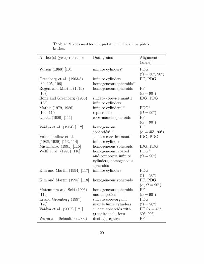
Table 4: Models used for interpretation of interstellar polar-ization.

Author(s) (year) reference Dust grains Alignment(angle)

Wilson (1960) [104] infinite cylinders∗ PDG(Ω = 30, 90)

Greenberg et al. (1963-8) infinite cylinders, PF, PDG[39, 105, 106] homogeneous spheroids∗∗

Rogers and Martin (1979) homogeneous spheroids PF[107] (α = 90)Hong and Greenberg (1980) silicate core–ice mantle IDG, PDG[108] infinite cylindersMathis (1979, 1986) infinite cylinders∗∗∗ PDG+

[109, 110] (spheroids) (Ω = 90)Onaka (1980) [111] core–mantle spheroids PF

(α = 90)Vaidya et al. (1984) [112] homogeneous PF

spheroids∗∗∗∗ (α = 45, 90)Voshchinnikov et al. silicate core–ice mantle IDG, PDG(1986, 1989) [113, 114] infinite cylindersMishchenko (1991) [115] homogeneous spheroids IDG, PDGWolff et al. (1993) [116] homogeneous, coated PDG+

and composite infinite (Ω = 90)cylinders, homogeneousspheroids

Kim and Martin (1994) [117] infinite cylinders PDG(Ω = 90)

Kim and Martin (1995) [118] homogeneous spheroids PF, PDG(α, Ω = 90)

Matsumura and Seki (1996) homogeneous spheroids PF[119] and ellipsoids (α = 90)Li and Greenberg (1997) silicate core–organic PDG[120] mantle finite cylinders (Ω = 90)Vaidya et al. (2007) [121] silicate spheroids with PF (α = 45,

graphite inclusions 60, 90)Wurm and Schnaiter (2002) dust aggregates PF

20

Table 4: (Continued.)

Author(s) (year) reference Dust grains Alignment(angle)

[122] consisting of 4–64 (α = 90)monomers

Voshchinnikov et al. (1990- homogeneous spheroids IDG, PDG2010) [66, 123, 124, 103]Draine and Fraisse (2009) oblate spheroids PDG++

[125] (Ω = 90)

PF — picket fence orientation

PDG — perfect Davis–Greenstein (2D) orientation

IDG — imperfect Davis–Greenstein orientation

α, (Ω) — angle between the line of sight and the direction of grain alignment in

the case of PF (PDG) orientation∗ in Rayleigh-Gans approximation;∗∗ in Rayleigh approximation;∗∗∗ efficiency factors tabulated by Wickramasinghe [126] were taken; polarization

for prolate spheroids was computed as for cylinders;∗∗∗∗ the figures of Asano [127] were used;+ large silicate grains are assumed to be perfectly aligned (see Eq. (18));++ only grains with sizes r > rcut are assumed to be perfectly aligned (see Eq. (19)).

Early models dealt with homogeneous infinitely long circular cylinders [105,106, 109, 110]4. This is the simplest model of non-spherical particles. So-lution to the light scattering problem for infinite cylinders was obtained bythe separation of variables method in the cylindrical coordinate system [128].Later, more advanced models with silicate core-ice mantle cylindrical parti-cles based on the solution from [129] were developed [108, 113, 114]. Theprogress in the light scattering theory allowed one to apply the model ofhomogeneous prolate and oblate spheroids of different size and shape for cal-culations of the polarizing efficiency, visual and UV polarization (see, e.g.,[107, 118, 103, 125]). Spheroidal particles are characterized by the aspectratio a/b where a and b are the major and minor semiaxes. The optical

4Another simplification was the use of the wavelength-independent refractive index.

21

properties of spheroids can be found by using different technique. The mostpopular methods widely applied in astronomical modelling are the separationof variables method [124, 130], the T-matrix method [115] and the discretedipole approximation [131]. Comparison of the methods and benchmarkresults are given in [132, 133]5. More complicated non-spherical particles(coated spheroids, ellipsoidal particles, composite spheroids) were consideredso far for illustrative calculations [111, 119, 121].

The polarization cross sections must be averaged over rotations takinginto account an alignment mechanism. According to standard concepts [1,134], the alignment of interstellar grains may be magnetic or radiative. A verypopular alignment mechanism is the magnetic alignment (Davis–Greenstein(DG) type orientation [135]) based on the paramagnetic relaxation of grainmaterial containing about one percent of iron impurities. For the imperfectDavis–Greenstein (IDG) orientation, the alignment function f(ξ, β) can bewritten as [108, 114]

f(ξ, β) =ξ sin β

(ξ2 cos2 β + sin2 β)3/2. (15)

The parameter ξ depends on the particle size rV , the imaginary part of thegrain magnetic susceptibility χ′′ (= κωd/Td, where ωd is the angular velocityof grain), gas density ng, the strength of magnetic field B and dust (Td) andgas (Tg) temperatures

ξ2 =rV + δ0(Td/Tg)

rV + δ0, where δIDG

0 = 8.23 1023 κB2

ngT1/2g Td

µm. (16)

If the grains are not aligned ξ = 1 and f(ξ, β) = sin β; in the case of theperfect rotational orientation ξ = 0. Unfortunately, only a limited number ofmodels including the combined particle size/shape/orientation analysis havebeen developed (see Table 4).

For simplicity, many investigators assumed that the direction of the mag-netic field (direction of grain alignment) was perpendicular to the line ofsight, i.e., α, Ω = 90 (e.g., [110, 118, 125]). Frequently, non-rotating parti-cles of the same orientation are considered (see Table 4). In this case, calledthe “picket fence” (PF) orientation, there are no integrals over the angles

5see also Database of Optical Properties (DOP): http://www.astro.spbu.ru/DOP

22

ϕ, ω and β in Eq. (14). The polarization degree is proportional to the polar-ization cross-section P ∝ Cpol = 1/2[CTM

ext (Ω) − CTEext (Ω)], where Ω = α and

f(ξ, β) = δ(α)6. The dichroic polarization efficiency is defined by the ratioof the polarization cross-section (factor) to the extinction one

(

P

τ

)

PF

=Cpol

Cext

=CTM

ext − CTEext

CTMext + CTE

ext

· 100% =QTM

ext −QTEext

QTMext +QTE

ext

· 100%. (17)

A more complicated case is the perfect rotational (2D) orientation (or perfectDavis–Greenstein orientation, PDG) when the major axis of a non-sphericalparticle always lies in the same plane. For the 2D orientation, integration isperformed over the spin angle ϕ only and f(ξ, β) = δ(β).

Polarization produced by perfectly aligned particles is much larger thanthat observed (cf. Figs. 9 and 10 with Eq. (11)). Nevertheless, the modelswith the PF or PDG orientation are useful for investigations of the normal-ized polarization (the Serkowski curves) as the wavelength dependence ofpolarization is only slightly influenced by the particle refractive index, sizeor shape (cf. left panels in Figs. 9 and 10). As a crude approximation of the

0 1 2 3 4 5 6 7 8 9 10

0

10

20

30

40

λ-1, µm-1

rV=0.05µm

rV=0.10µm

rV=0.15µm

P(λ

)/τ(λ

), %

astrosil, prolate, a/b=2, α=900

0 1 2 3 4 5 6 7 8 9 10

0

10

20

30

40

λ-1, µm-1

prolate, α=450

prolate, α=900

oblate, α=450

oblate, α=900

P(λ

)/τ(λ

), %

astrosil, a/b=2, rV=0.10µm

Figure 9: Wavelength dependence of the polarization efficiency for homogeneous spheroidsconsisting of astrosil for the PF orientation (see Eq. (17)). The effect of variations of theparticle size (left panel), type and orientation (right panel) is illustrated. Adapted from[2].

polarization efficiency for particles with the IDG orientation, the followingrelation is used (see, e.g., [107])

(

P

τ

)

IDG

= R sin2 Ω

(

P

τ

)

PF

,

6δ(z) is the Dirac delta function.

23

0 1 2 3 4 5 6 7 8 9 10

0

1

2

3

4

5

6

λ-1, µm-1

rV=0.05µm

rV=0.10µm

rV=0.20µm

rV=0.30µm

P(λ

)/A(λ

), %

astrosil, Ω=900

prolate, a/b=2, IDG, δ0=0.196µm

0 1 2 3 4 5 6 7 8 9 10

0

5

10

15

20

25

λ-1, µm-1

IDG, δ0=0.196µm

IDG, δ0=1.96µm

IDG, δ0=19.6µmPDG

P(λ

)/A(λ

), %

astrosil, Ω=900

prolate, rV=0.10µm,a/b=2 IDG, δ0=0.196µm

Figure 10: Wavelength dependence of the polarization efficiency for homogeneous rotatingspheroidal particles of the astronomical silicate. The effect of variations of particle size (leftpanel), and degree of alignment (right panel) is illustrated. The open circles and squaresshow the observational data for stars HD 24263 and HD 99264, respectively. Adaptedfrom [66].

where R = 1/2(3〈cos2 β〉 − 1) is the Rayleigh reduction factor [39, 136] and〈〉 denotes the ensemble average. It should be emphasized that applicationof this approximation as well as the Rayleigh reduction factor can lead tomisinterpretation of observational curves P (λ).

In the case of the IDG mechanism, smaller grains are aligned better thanlarger grains (see Eq. (16)). However, the models with an opposite type oforientation of small and large particles have been also suggested. Mathis [110]assumed that rotating silicate grains were perfectly aligned if they containat least one super-paramagnetic inclusion. Carbonaceous grains and silicategrains without inclusions are randomly oriented in space (3D orientation).The probability of perfect alignment is

f(rV , r′V ) = 1 − exp(−rV /r

′V )3. (18)

Draine and Fraisse [125] considered the model of silicate and amorphouscarbon spheroids with randomly oriented small particles and perfectly alignedlarge particles. In this case the alignment function is size dependent

f(β, rV ) =

sin β for rV ≤ rV, cut,δ(β) for rV > rV, cut,

(19)

where rV,cut is a cut-off parameter.Computations made by Das et al. [103] (see their Fig. 2) demonstrate

that the observational data can be fitted by using the models with different

24

alignment functions (e.g., given by Eqs. (15), (18) or (19)), especially if amore complex size distribution function as discussed in Sect. 2.2 is chosen.However, this complicates the model. To avoid the models with many pa-rameters new ideas about the nature of polarizing grains and physics of grainalignment should be included.

The DG mechanism of the paramagnetic relaxation requires a strongermagnetic field than average Galactic magnetic field (∼3 – 5µG; [137]). Be-cause of this problem, it has been suggested that the polarizing grains containsmall clusters of iron, iron sulfides, or iron oxides with super-paramagneticor ferromagnetic properties [138]. This leads to an enhancement of the imag-inary part of the magnetic susceptibility of grain material χ′′ by a factor 10– 100 and alignment can occur through the DG mechanism. This scenario issupported by laboratory experiments [139, 140]. A significant enhancementof χ′′ is also possible in mixed MgO/FeO/SiO grains [141] or in H2O icemantle grains containing magnetite (Fe3O4) precipitates [142, 143].

Another possibility to align interstellar grains is the radiative torquealignment (RAT alignment). It arises from an azimuthal asymmetry of thelight scattering by non-spherical particles. Magnetic inclusions can enhanceRAT alignment [144]. The theory of RAT alignment is well developed [145].Recent observations of interstellar polarization in the vicinity of luminousstars [146, 147, 148] have been used for confirmation of the RAT alignmentmechanism. However, the discussed models are phenomenological, they arenot based on correct light scattering calculations of interstellar polarization.One of the reasons is that the alignment function for the RAT mechanismis unknown. Another reason is a requirement of advanced light scatteringmethods because fast rotation can only occur for grains of very specific (he-lical) shape [145, 149]. This is highly improbable from the point of view ofgrain growth in the interstellar medium.

Since both magnetic alignment and radiative alignment depend on ironinclusions, we can expect that polarization and/or polarization efficiencyshould increase with the growth of iron fraction in dust grains. This ideawas investigated by Voshchinnikov et al. [150] by using available data oninterstellar polarization and element abundances previously compiled in [29].It was suggested that the interstellar polarization was probably related to theamount of iron in dust grains. Assuming that all silicon and all magnesiumare embedded into amorphous silicates of olivine composition (Mg2xFe2−2xSiO4,where x = [Mg/H]d/(2[Si/H]d) as is a part of iron. The remaining part of Fe

25

can be found as

[Fe(rest)/H]d = [Fe/H]d − (2 [Si/H]d − [Mg/H]d). (20)

As indicated in Fig. 11 (left panel), there is a negative correlation between

Figure 11: Interstellar polarization in dependence on remaining dust phase abundance ofFe as given by Eq. (20) (left panel) and dust phase abundance of silicon (right panel).Halo stars with |b| > 30 and disk stars with |b| ≤ 30 and low (E(B − V ) ≤ 0.2) andhigh (E(B − V ) > 0.2) reddening are shown with different symbols. Number of stars isindicated in parentheses in the legend. Adapted from [150].

the polarization degree P and the amount of remaining iron. This is incon-sistent with the common suggestion about the great role of iron-rich grains inthe production of polarization. Since P is proportional to the column densityof polarizing grains, we can conclude that the increase of the iron content innon-silicate grains does not enhance polarization.

Because in calculating [Fe(rest)/H]d we removed all Si and Mg and apart of Fe from the dust phase, we expect a positive correlation betweenthe polarization and the abundances of the eliminated elements. There isonly a weak correlation between P and [Fe/H]d or [Mg/H]d (see [150] formore discussion) and a strong correlation between P and [Si/H]d (Fig. 11,right panel). Therefore, it can be established that polarization is more likelyproduced by silicates. These findings are evidence in favour of the assumptionof Mathis [110] that only the silicate grains are aligned and contribute to the

26

observed polarization, while the carbonaceous grains are either spherical orrandomly aligned. Another verification of this suggestion is the absence ofany correlation between the polarization efficiency P/E(B−V ) or P/AV anddust phase abundances of elements (see [150]). This is because dust grains ofall types (silicate, carbonaceous, iron-rich, etc.) contribute to the observedextinction, while only the silicates seems to be responsible for the observedpolarization. Thus, the absence of correlation between RV and λmax (seediscussion in Sect. 3.1) can be easily understood. These discoveries can beexplained if the silicate grains aligned by the radiative mechanism are mainlyresponsible for the observed interstellar linear polarization7.

Analysing models presented in Table 4, it is possible to say that the majorpart of models includes perfect grain alignment and one angle of alignmentand merely a few of them with the IDG orientation can be used for inter-pretation of observations of individual stars. Indeed, the previous modellingof interstellar polarization was mainly focused on the explanation of the av-erage wavelength dependence (Serkowski curve) [109, 110, 117, 118]. OnlyLi and Greenberg [69] applied their model of coated cylinders to explainthe normalized polarization curve in the direction of HD 210121 and Daset al. [103] interpreted interstellar extinction and polarization observationsof seven stars using a mixture of carbonaceous and silicate spheroids. Thisfact causes deep dissatisfaction because a great amount of observations ofinterstellar polarization in different areas exists and continuously grows.

3.3. Interpretation: dust grains and magnetic field in the Taurus dark cloud

In this section we present the quantitative interpretation of observationsof interstellar polarization for a group of stars8. Our model of spheroidalgrains with imperfect alignment [66, 103] is supplemented by the subroutinecalculating three parameters of the Serkowski curve. We also assume thatpolarization is mainly produced by silicate grains and the degree of alignmentof carbonaceous grains is small (see discussion in previous section).

As an example we refer to the Taurus dark cloud (TDC) — the complex ofinterstellar clouds where active star formation is in progress. This complex

7Polarization in IR features also supports the idea of separate populations of polarizing(silicate) and non-polarizing (carbonaceous) grains. This follows from the observed polar-ization of silicate features at 10 µm and 18 µm and the lack of polarization in the 3.4 µmhydrocarbon feature (see [151, 152] and references therein).

8More detailed discussion can be found in [86].

27

lies sufficiently far from the Galactic plane (b ≈ −15) at a distance of∼ 140 pc and comprise several dozens dark nebulae, clouds and clumps [153,154]. It suffers negligible foreground and background extinction [155, 156]and is the subject of numerous investigations of molecular gas [157, 158, 159,160, 161].

The polarimetric observations of several hundreds stars in the regionaround the Taurus dark cloud complex have been performed at visual andred wavelengths [160, 162, 163] and in the H and K bands [95, 164, 165, 166].The obtained polarization maps give an insight into the structure of theplane-of-the-sky component of interstellar magnetic field but are of littleuse for studies of grain properties and alignment. To find these latter, thewavelength dependence of polarization must be involved. Whittet et al. [82]presented the polarimetric and photometric observations of 27 stars in a widespectral range in the TDC (l ≈ 170÷ 176, b ≈ –10÷ –17) and calculatedthe fit parameters of the Serkowski curve Pmax, λmax and K as well as the val-ues of RV . Our initial analysis of these data is based on the two-componentmodel of Messenger et al. [101] and Whittet et al. [167] (see also discussionof Table 3 in Sect. 3.1). It made possible to form two groups of stars withrelatively uniform distribution of positional angles of polarization: cloud 1(14 stars, θgal. = 145 − 175) and cloud 2 (13 stars, θgal. = 2 − 40).

Firstly, we should concentrate on stars in cloud 1 located inside or be-hind the “diffuse–screen” component of the TDC. These stars are distributedaround Heiles Cloud 2 (l ≈ 174.4, b ≈ –13.4, area 15.8 pc2 [161]) — a densecondensation containing TMC-1 (Taurus molecular cloud). Observationaldata for stars in the cloud 1 plotted in Figs. 12, 13 indicate positive correla-tion between K and λmax (the width of the polarization curve W decreaseswith increasing λmax) and negative correlation between the polarization effi-ciency Pmax/AV and λmax. The first dependence is well known (see Fig. 6 anddiscussion in [84]). Its qualitative explanation is a systematic reduction inthe relative number of small, aligned grains in regions of high λmax [82, 90].The sole quantitative modelling was attempted by Aannestad and Greenberg[168]. However, to reduce computational efforts they ruled out the integra-tion over the angle ω in Eqs. (14) which led to wrong results for W [114].A systematic trend toward smaller polarizing efficiency for larger λmax wasdetected for nearby stars closely located on the sky [82, 88, 89]. It has beeninterpreted as a result of the decrease of the angle Ω between the directionof the magnetic field and the line of sight [114].

The results of theoretical modelling are shown in Figs. 12, 13 by open cir-

28

0.4 0.5 0.6 0.7 0.8

0.5

1.0

1.5

cloud 1 (stars with θgal=145o-175o)

models

1

3

4

5

6

7

8

9

10

11

12

13

14-1

-1.5

-2

-2.5

-3

-0.5

1530

45

607590

2

λmax, µm

K rcorr.=0.656

0.4 0.5 0.6 0.7 0.8

0.5

1.0

1.5

cloud 1 (stars with θgal.=145o-175o)

models

1

3

4

5

6

7

8

9

10

11

12

13

14

0.07

0.030.05

0.09

0.1

0.12 153045607590

2

λmax, µm

K rcorr.=0.656

Figure 12: The coefficients K of the Serkowski curve (10) in dependence on the wavelengthof maximum polarization λmax for 14 stars in cloud 1 in Taurus with the similar positionalangles of polarization. The numbers of stars correspond to the increasing HD numbersof stars in Fig. 6, i.e. 1 = HD 28225, . . . , 14 = HD 283879. The Pearson correlationcoefficient between K and λmax is given. Open circles with line show model calculationswith different alignment angles Ω = 15(15)90. The values of Ω increase from right toleft as marked for the top model. Left panel illustrates the effect of variations of the powerindex q in the power-law size distribution (q varies from –0.5 to –3). Right panel illustratesthe effect of variations of the lower cut-off rV,min in the power-law size distribution (rV,min

varies from 0.03µm to 0.12µm). Other model parameters are: prolate spheroids, a/b = 3,rV,max = 0.35µm, rV,min = 0.07µm (left panel), q = −2 (right panel).

cles connected with solid line. The particle shape was fixed: prolate spheroidswith the aspect ratio a/b = 3. Under assumptions made the main parametersof our model influencing the polarization are: the lower and upper cut-offsrV,min and rV,max and the power index q in the power-law size distribution forsilicate particles and the degree (parameter δIDG

0 , see Eq. (16)) and direction(angle Ω) of alignment. Left and right panels in Fig. 12 illustrate the vari-ations of the index q and lower cut-off rV,min, respectively. The rise of theseparameters may be associated with the growth of dust grains by coagulation(q) or accretion (rV,min). In both cases the mean size of grains is bigger atthe right upper corner of Fig. 12 in comparison with its left bottom corner.It is interesting that the stars NN 1, 5, 6, 8, 11, 14 located at the right uppercorner apparently are embedded in Heiles Cloud 2 or situated at its boundary

29

0.4 0.5 0.6 0.7 0.8

0

1

2

3

4

5

cloud 1 (stars with θgal=145o-175o)

models

1

3

4

56

7

8

9

10

11

12

13

14

-2.5

-3

-2

-1.5-1 -0.5

15

30

45

60

75

90

2

Pm

ax/A

V, %

λmax, µm

rcorr=-0.735

0.4 0.5 0.6 0.7 0.8

0

1

2

3

4

5

cloud 1 (stars with θgal=145o-175o)

models

1

3

4

56

7

8

9

10

11

12

13

14

0.070.10.03 0.12

15

30

45

60

75

90

2

Pm

ax/A

V, %

λmax, µm

rcorr=-0.735

Figure 13: The polarizing efficiency Pmax/AV in dependence on the wavelength of maxi-mum polarization λmax for 14 stars in cloud 1 in Taurus. The Pearson correlation coeffi-cient between Pmax/AV and λmax is given. Open circles with line show model calculationswith different alignment angles Ω = 15(15)90. The values of Ω increase from bottomto top as marked for the right model. Left panel illustrates the effect of variations ofthe power index q in the power-law size distribution (q varies from –0.5 to –3). Rightpanel illustrates the effect of variations of the lower cut-off rV,min in the power-law sizedistribution (rV,min varies from 0.03µm to 0.12µm). Other model parameters are: prolatespheroids, a/b = 3, rV,max = 0.35µm, rV,min = 0.07µm (left panel), q = −2 (right panel).

(see Fig. 14). Note also that variations of alignment parameters δIDG0 and Ω

only do not allow explaining the observed correlation between K and λmax.The opposite situation occurs with the correlation between the polariza-

tion efficiency Pmax/AV and λmax (Fig. 13). In this case to explain bothhigh and low values of Pmax/AV it is not sufficient to change the grain sizeonly, variations of parameters δIDG

0 and Ω must be taken into account. Thetheoretical points plotted in Fig. 13 were obtained for δIDG

0 = 3µm. Smallervalues of δIDG

0 do not reproduce the data for directions with high polarizationefficiency (stars NN 2, 3, 10). It is evident that the obtained grain parametersare model-dependent (e.g., it is possible to use particles of another shape).However, with our model of interstellar dust the trends in variations of thegrain size, shape, alignment can be determined.

We attribute the variations of Pmax/AV in Fig. 13 to the changes in thedirection of magnetic field (direction of grain alignment). Stars can be di-

30

176 174 172 170

-16

-14

-12

-10

Ω=300-450

Ω=450-600

Ω=600-900

Turner, Heiles, 2006 (C4H, Zeeman)

Crutcher et al., 2010 (OH, Zeeman)

6

5

4

7

14

11

1

8

12

13

9

102

3

L1521

B217-2L1521E

TMC-1

B18-5

B220L1534

l, deg.

b, d

eg.

2%

Figure 14: Linear polarization map of the cloud 1 in Taurus containing 14 stars with similarpositional angles. The lengths of the lines are proportional to the percent polarization.The sizes of the circles are proportional to the alignment angle Ω. The dashed contourrepresents the regions with different visual extinction: 1.m6 < AV < 19.m6 inside contourand 0.m4 < AV < 1.m6 outside contour [156, 169]. The cross corresponds to the clump inTMC-1 where Turner and Heiles [170] have searched the C4H Zeeman effect. The opencircles show the positions of dark clouds where the OH Zeeman effect has been observed[171].

vided into three groups with close values of Ω (see right panel in Fig. 13).These groups of stars are shown in Fig. 14 by filled circles of different sizes.This Figure gives the positions and polarization of stars in cloud 1 and ap-proximate contours of Heiles Cloud 2. It is intriguing that all six stars withthe larger values of Ω (the magnetic field is mainly perpendicular to the lineof sight) are closely located on the sky outside of Heiles Cloud 2. Other eightstars where the magnetic field is significantly tilted to the line of sight aresituated near the boundary of the cloud. An indirect support to our interpre-tation is provided by Zeeman observations. Turner and Heiles [170] obtainedan upper limit for magnetic field toward the cold dense TMC-1 cyanopolyynepeak core B‖ = B cos Ω = 14.5 ± 14µG. A possible reason for this result is

31

that the magnetic field is directed close to the plane of the sky. Crutcher etal. [171] compiled the Zeeman data for many dark clouds. Several of themlocated near or inside Heiles Cloud 2 are marked as large open circles inFig. 14. In almost all cases the data are within 1σ error. Only for B217-2(close to the positions of stars NN 5, 6) the component of the magnetic fieldparallel to the line of sight has been detected (B‖ = 13.5 ± 3.7µG).

The structure and evolution of magnetic field in Heiles Cloud 2 have beendiscussed by Heyer et al. [160] and Tamura et al. [164]. It was suggested thatthe contraction and formation of the cloud from the placental Taurus darkcloud with homogeneous magnetic structure occurred along the magneticfield. The gas motions in Heiles Cloud 2 can be described in terms of arotating ring with the rotation axis coinciding with the magnetic field [157].Our findings infer that the magnetic field is tilted with respect to the line ofsight at the boundaries of Heiles Cloud 2, i.e., magnetic field has a spindel-like structure. Apparently, the area disturbed by contraction of Heiles Cloud2 terminates at the place where the magnetic field is almost perpendicularto the line of sight (stars NN 2, 3, 9, 10, 12, 13).

4. Conclusions

All modern investigations of cosmic dust in protoplanetary disks, denseclouds, distant galaxies are based on the modelling of “classical” observationsof the interstellar extinction and polarization. Our examination shows thatthe interpretation of these basic observations still remains incomplete. Newgeneration models should include a consideration of interstellar abundancesin given directions and accurate treatment of light scattering by physicallyfeasible particles with realistic alignment.

Acknowledgments

I am grateful to organizers F. Borghese, M.A. Iatı and R. Saija for invitingme to present this review. I am thankful to the referees for useful comments,L. Cambresy and P. Padoan for sending the extinction map in numerical form,I.S. Yakovlev and H.K. Das for assistance in calculations and to V.B. Il’in forproduction Serkowski fitting subroutine and careful reading of manuscript.The work was partly supported by the grant RFBR 10-02-00593a of theRussian Federation.

32

References

[1] Whittet DCB. Dust in the Galactic Environments. 2nd ed. Bristol:Institute of Physics Publishing; 2003.

[2] Voshchinnikov NV. Optics of Cosmic Dust. I. Astrophys Space PhysRev 2004;12:1–182.

[3] Witt AN, Clayton GC, Draine BT, editors. Astrophysics of Dust. ASPConf. Ser. 309, 2004.

[4] Henning Th, Grun E, Steinacker J, editors. Cosmic Dust – Near andFar. ASP Conf. Ser. 414, 2009.

[5] Henning Th, editor. Astromineralogy. 2nd ed. Heidelberg: Springer;Lect Notes Phys 815, 2010.

[6] Dorschner J. From dust astrophysics towards dust mineralogy — ahistorical review. In: Henning Th, editor. Astromineralogy, 2nd ed.Heidelberg: Springer; 2010, Lect Notes Phys 815, p. 1–60.

[7] Li A. Interstellar Grains — The 75th Anniversary. In: Saija R, Cecchi-Pestellini C, editors, Light, Dust and Chemical Evolution. Bristol: In-stitute of Physics Publishing; J. Phys. Conf. Ser. 2005;6:229–248.

[8] Fitzpatrick EL, Massa DL. An Analysis of the Shapes of InterstellarExtinction Curves. V. The IR-Through-UV Curve Morphology. Astro-phys J 2007;663:320–341.

[9] Voshchinnikov NV, Il’in VB. Interstellar extinction curve in the far andextreme ultraviolet. Sov Astron 1993;37:21–25.

[10] Martin PG, Whittet DCB. Interstellar extinction and polarization inthe infrared. Astrophys J 1990; 357:113–124.

[11] Fitzpatrick EL, Massa DL. An Analysis of the Shapes of Interstel-lar Extinction Curves. VI. The near-IR exctinction law. Astrophys J2009;699:1209–1222.

[12] Indebetouw R, Mathis JS, Babler BL, Meade MR, Watson C, WhitneyBA. et al. The wavelength dependence of interstellar extinction from1.25 to 8.0 µm using GLIMPSE data. Astrophys J 2005;619:931–938.

33

[13] Fritz TK, Gillessen S, Dodds-Eden K, Lutz D, Genzel R, Raab W. et al.The derived infrared extinction toward the Galactic center. AstrophysJ 2011;737:73(21pp).

[14] Valencic LA, Clayton GC, Gordon KD. Ultraviolet extinction proper-ties in the Milky Way. Astrophys J 2004;616:912–924.

[15] Gordon KD, Cartledge S, Clayton GC. FUSE measurements of far-ultraviolet extinction. III. The dependence on R(V ) and discrete fea-ture limits from 75 Galactic sightlines. Astrophys J 2009;705:1320–1335.

[16] Fitzpatrick EL, Massa DL. An Analysis of the Shapes of InterstellarExtinction Curves. I. The 2175 A bump. Astrophys J 1986;307:286–294.

[17] Dorschner J. Properties of the λ 2200 A interstellar absorber. Astro-phys Sp Sci 1973;25:405–411.

[18] Fitzpatrick EL, Massa DL. An Analysis of the Shapes of InterstellarExtinction Curves. III. An atlas of ultravilet extinction curves. Astro-phys J Suppl Ser 1990;72:163–189.

[19] Cardelli JA, Clayton GC, Mathis JS. The determination of ultravioletextinction from optical and near–infrared. Astrophys J 1988;329:L33–L37.

[20] Cardelli JA, Clayton GC, Mathis JS. The relationship between in-frared, optical, ultraviolet extinction. Astrophys J 1989;345:245–256.

[21] Kre lowski J, Wegner W. Interstellar exctinction curves originated insingle clouds. Astron Nachr 1989;310:281–287.

[22] Mazzei P, Barbaro G. Dust properties along anomalous extinctioncurves. Mon Not R Astron Soc 2008;390:706–714.

[23] Mazzei P, Barbaro G. Dust properties along anomalous extinctioncurves. II. Studying extinction curves with dust models. Astron As-trophys 2011;527:A34(16pp).

[24] Zonca A, Cecchi-Pestellini C., Mulas G, Malocci G. Modelling peculiarextinction curves. Mon Not R Astron Soc 2011;410:1932–1938.

34

[25] Kre lowski J, Strobel A. Limited diversity of the interstellar extinctionlaw. Astron Nachr 2012;333:60–70.

[26] Rai RK, Rastogi S. Modeling anomalous/non-CCM extinction usingnanodiamonds. Mon Not R Astron Soc 2012; doi: 10.1111/j.1365-2966.2012.21109.x.

[27] Gudennavar SB, Bubbly SG, Preethi K, Murthy J. A compilation ofinterstellar column densities. Astrophys J Suppl Ser 2012;199:8(14pp).

[28] Jenkins EB. A unified representation of gas-phase elemet depletions inthe interstellar medium. Astrophys J 2009;700:1299–1348.

[29] Voshchinnikov NV, Henning Th. From interstellar abundances to graincomposition: the major dust constituents Mg, Si, and Fe. Astron As-trophys 2010;517:A45(15pp).

[30] Parvathi VS, Sofia UJ, Murthy J, Babu SRS. Understanding the roleof carbon in ultraviolet extinction along Galactic sight lines. AstrophysJ 2012;in press.

[31] Weingartner JC, Draine BT. Dust grain-size distribution and extinc-tion in the Milky Way, Large Magellanic Cloud, and Small MagellanicCloud. Astrophys J 2001;548:296–309.

[32] Li A, Draine BT. Infrared emission from interstellar dust. II. The dif-fuse interstellar medium. Astrophys J 2001;554:778–802.

[33] Cecchi-Pestellini C, Malocci G, Mulas G, Joblin C, Williams DA. Therole of the charge state of PAHs in ultraviolet extinction. Astron. As-trophys 2008;486:L25–L29.

[34] Clayton GC, Gordon KD, Salama F, Allamandola LJ, Martin PG,Snow TP. et al. The role of polycyclic aromatic hydrocarbons in ultra-violet extinction. I. Probing small molecular polycyclic aromatic hy-drocarbons. Astrophys J 2003;592:947–952.

[35] Gredel R, Carpenter Y, Rouille G, Steglich M, Huisken F, HenningTh. Abundances of the PAHs in the ISM: confronting observationswith experimental results. Astron. Astrophys 2011;530:A26(15pp).

35

[36] Greenberg JM. Interstellar Grains. In: McDonnell JAM, editor. CosmicDust, New York: Wiley; 1978, p. 187–294.

[37] Cecchi-Pestellini C, Cacciola A, Iatı MA, Saija R, Borghese F, DentiP. et al. Stratified dust grains in the interstellar medium – II. Time-dependent interstellar extinction. Mon Not R Astron Soc 2010;408:535–541.

[38] Oort JH, van de Hulst HC. Gas and smoke in interstellar space. BullAstron Inst Netherlandes 1946;10:187–204.

[39] Greenberg JM. Interstellar Grains. In: Middlehurst BM, Aller LH, ed-itors. Stars and Stellar Systems, Vol. VII, Chicago: Univ. ChicagoPress; 1968, p. 221–364.

[40] Isobe S. Evaporation of dirty ice particles surrounding early type stars.IV. Various size distributions. Publ Astron Soc Japan 1973;25:101–109.

[41] Mathis JS, Rumpl W, Nordsieck KH. The size distribution of interstel-lar grains. Astrophys J 1977;217:425–433.

[42] Wickramasinghe NC, Guillaume C. Interstellar extinction by graphitegrains. Nature 1965;207:366–368.

[43] Wickramasinghe NC, Nandy K. Optical properties of graphite–iron–silicate grain mixtures. Mon Not R Astron Soc 1971;153:205–227.

[44] Wickramasinghe NC, Nandy K. Recent work on interstellar grains. RepProgr Phys 1972;35:157–234.

[45] Kim S-H, Martin PG, Hendry PD. The size distribution of inter-stellar dust particles as determined from extinction. Astrophys J1994;422:164–175.

[46] Mathis JS. Dust models with tight abundance constraints. AstrophysJ 1996;472:643–655.

[47] Zubko VG, Dwek E, Arendt G. Interstellar dust models consistent withextinction, emission, and abundance constraints. Astrophys J Suppl Ser2004;152:211–249.

36

[48] Zubko VG, Kre lowski J, Wegner W. The size distribution of dust grainsin single clouds — I. The analysis of extinction using multicomponentmixtures of bare spherical grains. Mon Not R Astron Soc 1996;283:577–588.

[49] Zubko VG, Kre lowski J, Wegner W. The size distribution of dust grainsin single clouds — II. The analysis of extinction using inhomogeneousgrains. Mon Not R Astron Soc 1998;294:548–556.

[50] Wickramasinghe NC. On graphite particles as interstellar grains, II.Mon Not R Astron Soc 1963;126:99–114.

[51] Wickramasinghe NC. Extinction curves for graphite–silicate grain mix-tures. In: Houziaux L, Butler HE, editors. Ultraviolet stellar spectraand ground based observations, Dordrecht: Reidel; 1970; IAU Symp36:42–49.

[52] Greenberg JM, Li A. The core–mantle interstellar dust model. In:Greenberg JM, editor, The Cosmic Dust Connection, Dordrecht:Kluwer; 1996, p. 43–70.

[53] Dorschner J, Henning Th. Dust metamorphosis in the galaxy. AstronAstrophys Rev 1995;6:271–333.

[54] Farafonov VG, Il’in VB. Single light scattering: computational meth-ods. In: Kokhanovsky AA, editor. Light Scattering Reviews, Berlin:Springer; 2006, vol. 1, p. 125–177.

[55] Borghese F, Denti P, Saija R. Scattering by model non-spherical par-ticles. 2nd ed. Heidelberg: Springer; 2007.

[56] Min M. Optical properties of dust grains in the infrared: our view oncosmic dust. In: Henning Th, Grun E, Steinacker J, editors. CosmicDust – Near and Far, 2009, ASP Conf. Ser. vol. 414, p. 356–371.

[57] Mathis JS, Whiffen G. Composite interstellar grains. Astrophys J1989;341:808–822.

[58] Vaidya DB, Gupta R, Dobbie JS, Chylek P. Interstellar extinction bycomposite grains. Astron Astrophys 2001;375:584–590.

37

[59] Gupta R, Mukai T, Vaidya DB, Sen AK, Okada Y. Interstellar extinc-tion by spheroidal dust grains. Astron Astrophys 2005;441:555–561.

[60] Voshchinnikov NV, Mathis JS. Calculating Cross Sections of CompositeInterstellar Grains. Astrophys J 1999;526:257–264.

[61] Voshchinnikov NV, Il’in VB, Henning Th, Dubkova DN. Dust extinc-tion and absorption: the challenge of porous grains. Astron Astrophys2006;445:167–177.

[62] Iatı MA, Cecchi-Pestellini C, Williams DA, Borghese F, Denti P, SaijaR. et al. Stratified dust grains in the interstellar medium – I. An ac-curate computational method for calculating their optical properties.Mon Not R Astron Soc 2008;384:591–598.

[63] Farafonov VG, Voshchinnikov NV. Light scattering by a multilayeredspheroidal particle. Appl Opt 2012;51:1586–1597.

[64] Voshchinnikov NV, Il’in VB, Henning Th. Modelling the optical prop-erties of composite and porous interstellar grains. Astron Astrophys2005;429:371–381.

[65] Li A. Can fluffy dust alleviate the subsolar interstellar abundance prob-lem? Astrophys J 2005;622:965–969.

[66] N.V. Voshchinnikov, and H.K. Das, Modelling interstellar extinctionand polarization with spheroidal grains. J Quantitative Spectrosc RadTransfer 2008;109:1527–1537.

[67] Chini R, Krugel E. Abnormal extinction and dust properties in M 16,M 17, NGC 5357 and the Ophiuchus dark cloud. Astron Astrophys1983;117:289–296.

[68] Aannestad PA. Ultraviolet extinction to 10.8 inverse microns. Astro-phys J 1995;443:653–663.

[69] Li A, Greenberg JM. The dust extinction, polarization and emis-sion in the high-latitude cloud toward HD 210121. Astron Astrophys1998;339:591–600.

38

[70] Larson KA, Wolff MJ, Roberge WG, Whittet DCB, He L. The sizedistribution of dust toward HD 210121 as determined from extinction.Astrophys J 2000;532:1021–1028.

[71] Clayton GC, Wolff MJ, Sofia UJ, Gordon KD, Misselt KA. Dust grainsize distributions from MRN to MEM. Astrophys J 2003;588:871–880.

[72] Jones AP, Duley WW, Williams DA. The structure and evolution ofhydrogeneted amorphous carbon grains and mantles in the interstellarmedium. Quart J Roy Astron Soc 1990;31:567–582.

[73] Cecchi-Pestellini C, Iatı MA, Williams DA. The nature of interstellardust as revealed by light scattering. this issue.

[74] Hiltner WA. Polarization of light from distant stars by interstellarmedium. Science 1949;109:165–165.

[75] Hall JS. Observations of the polarized light from stars. Science1949;109:166–167.

[76] Dombrovskii VA. On the polarization of radiation of early-type stars.Doklady Akad Nauk Armenia. 1949;10:199–203.

[77] Serkowski K. Interstellar polarization. In: Greenberg JM, Hayes DS,editors, Interstellar Dust and Related Topics, Dordrect: Reidel; 1973,IAU Symp vol. 52, p. 145–152.

[78] Serkowski K, Mathewson DS, Ford VL. Wavelength dependence of in-terstellar polarization and ratio of total to selective extinction. Astro-phys J 1975;196:261–290.

[79] Wolstencroft RD, Smith RJ. High precision spectropolarimetry of starsand olanets — III. The wavelength dependence of interstellar polariza-tion. Mon Not R Astron Soc 1984;208:461–480.

[80] Efimov YuS. Interstellar polarization: new approximation. Bull CrAO2009;105:82–114.

[81] Whittet DCB, van Breda IG. The correlation of the interstellar extinc-tion law with the wavelength of maximum polarization. Astron Astro-phys 1978;66:57–63.

39

[82] Whittet DCB, Gerakines PA, Hough JH, Shenoy SS. Interstellar ex-tinction and polarization in the Taurus dark clouds: the optical prop-erties of dust near the diffuse/dense cloud interface. Astrophys J2001;547:872–884.

[83] Andersson B-G, Potter SB. Observational constraints on interstellargrain alignment. Astrophys J 2007;665:369–389.

[84] Whittet DCB, Martin PG, Hough JH, Rouse MF, Bailey JA, AxonDJ. Systematic variations in the wavelength dependence of interstellarlinear polarization. Astrophys J 1992;386:562–577.

[85] Martin PG, Adamson AJ, Whittet DCB, Hough JH, Bailey JA, Kim S-H. et al. Interstellar polarization from 3 to 5 microns in reddened stars.stars with extreme values of λmax. Astrophys J 1992;392:691–701.

[86] Voshchinnikov NV, Yakovlev IS, Il’in VB, Das HK. Serkowski polar-ization curve calibrated with spheroidal grains. Mon Not R Astron Soc2012; in preparation.

[87] Rodrigues CV, Sartori MJ, Gregorio-Hetem J, Magalhaes M. The align-ment of the polarization Herbig Ae/Be stars with interstellar magneticfield. Astrophys J 2008;698:3031–2035.

[88] Whittet DCB, Gerakines PA, Carkner AL, Hough JH, Martin PG,Prusti T. et al. A study of the Chamaeleon I dark cloud and T-association – VI. Interstellar polarization, grain alignment and mag-netic field. Mon Not R Astron Soc 1994;268:1–12.

[89] Voshchinnikov NV, Yakovlev IS. The relationship between grain shapeand interstellar polarization. In: Muinonen K, Pehnttila A, LindquistH, Nousiainen T, Videen G, editors, Electromagnetic and Light Scat-tering: Theory and Applications, XII, Helsinki: University of Helsinki;2010, p. 318–321.

[90] Martin PG, Clayton GC, Wolff MJ. Ultraviolet interstellar linear polar-ization. V. Analysis of the final data set. Astrophys J 1999;510:905–914.

[91] Wilking BA, Lebofsky MJ, Kemp JC, Martin PG, Rieke GH. Thewavelength dependence of interstellar linear polarization. AstrophysJ 1980;235:905–910.

40

[92] Andersen CM, Weitenbeck AJ, Code AD, Nordsieck KH, Meade MR,Babler BL. et al. Ultraviolet interstellar linear polarization of galacticstarlight I. Observations by the Wisconsin Ultraviolet Photo Polarime-ter Experiment. Astronom J 1996;112:2726–2743.

[93] Goodman AA, Jones TT, Lada EA, Myers PC. Does near–infraredpolarimetry reveal the magnetic field in cold dark cloud? Astrophys J1995;448:748–765.

[94] Arce HG, Goodman AA, Bastien P, Manset N, Sumner M. The po-larizing power of the interstellar medium in Taurus. Astrophys J1998;499:L93–L97.

[95] Gerakines PA, Whittet DCB, Lazarian A. Grain alignment in Taurusdark cloud. Astrophys J 1995;455:L71–L75.

[96] Whittet DCB. Polarization observations of molecular clouds. In:Adamson A, Aspin C, Davis CJ, Fujiyoshi T, editors, Astronomical Po-larimetry: current status and future directions. ASP Conf. Ser. 2005;v. 343: p. 321–331.

[97] Whittet DCB, Hough JH, Lazarian A, Hoang T. The efficiency of grainalignment in dense interstellar clouds: a reassessment of constraintsfrom near-infrared polarization. Astrophys J 2008;674:304–315.

[98] Lazarian A, Goodman AA, Myers PC. On the efficiency of grain align-ment in dark clouds. Astrophys J 1997;490:273–280.

[99] Hough JH, Sato S, Tamura M, Yamashita T, McFadzean AD, RouseMF. et al. Sectropolarimetry of the 3-µm ice band in Elias 16 (TaurusDark Cloud). Mon Not R Astron Soc 1988;230:107–115.

[100] Hough JH, Aitken DK, Whittet DCB, Adamson AJ, Chrysostomou A.Grain alignment in dense cold environments: spectropolarimetry of the4.67 µm CO-ice feature in the field star Elias 16 (Taurus dark cloud).Mon Not R Astron Soc 2008;387:797–802.

[101] Messenger DW, Whittet DCB, Roberge WG. Interstellar polarizationin the Taurus dark clouds: wavelength–dependent position angles andcloud structure near TMC-1. Astrophys J 1997;487:314–319.

41

[102] Bohren CF, Huffman DR. Absorption and Scattering of Light by SmallParticles. John Wiley and Sons: New York: 1983.

[103] Das HK, Voshchinnikov NV, Il’in VB. Interstellar extinction and po-larization – A spheroidal dust grain approach perspective. Mon Not RAstron Soc 2010;404:265–274.

[104] Wilson R. The relation between interstellar extinction and polarization.Mon Not R Astron Soc 1960;120:51–63.

[105] Greenberg JM, Lind AC, Wang RT, Libelo LF. The polarization ofstarlight by oriented nonspherical particles. In: Kerker M, editor, Elec-tromagnetic Scattering. New York: Pergamon Press; 1963; p. 123–134.

[106] Greenberg JM, Shah G. A unified model of interstellar extinction andpolarization. I. Astrophys J 1966;145:63–74.

[107] Rogers C, Martin PG. On the shape of interstellar grains. Astrophys J1979;228:450–464.

[108] Hong SS, Greenberg JM. A unified model of interstellar grains: aconnection between alignment efficiency, grain model size, and cosmicabundance. Astron Astrophys 1980;88:194–202.

[109] Mathis JS. The size distribution of interstellar grains. II. Polarization.Astrophys J 1979;232:747–753.

[110] Mathis JS. The alignment of interstellar grains. Astrophys J1986;308:281–287.

[111] Onaka T. Light scattering by spheroidal grains. Ann Tokyo Astron Obs1980;18:1–54.

[112] Vaidya DB, Bhatt HC, Desai JN. Interstellar extinction and polariza-tion by spheroidal dust grains. Astrophys Space Sci 1984;104:323–336.

[113] Voshchinnikov NV, Il’in AE, Il’in VB. Light extinction and polariza-tion by dust grains in the interstellar medium: the interstellar linearpolarization. Astrophysics 1986;24:299–305.

42

[114] Voshchinnikov NV. Determination of and magnetic fields from po-larimetric and photometric observations of stars. Astron Nachr1989;310:265–271.

[115] Mishchenko MI. Extinction and polarization of transmitted light bypartially aligned nonspherical grains. Astrophys J 1991;367:561–574.

[116] Wolff MJ, Clayton GC, Meade MR. Ultraviolet interstellar linearpolarization I. Applicability of current grain models. Astrophys J1993;403:722–735.

[117] Kim S-H, Martin PG. The size distribution of interstellar dust parti-cles as determined from polarization: infinite cylinders. Astrophys J1994;431:783–796.

[118] Kim S-H, Martin PG. The size distribution of interstellar dust particlesas determined from polarization: spheroids. Astrophys J 1995;444:293–305.

[119] Matsumura M, Seki M. Extinction and polarization by ellipsoidal par-ticles in the infrared. Astrophys J 1996;456:557–565.

[120] Li A, Greenberg JM, A unified model of interstellar dust. Astron As-trophys 1997;323:566–584.

[121] Vaidya DB, Gupta R, Snow TP. Composite interstellar grains. MonNot R Astron Soc 2007;379:791–800.

[122] Wurm G, Schnaiter M. Coagulation as unifying element for interstellarpolarization. Astrophys J 2002;567:370–375.

[123] Voshchinnikov NV. Optical properties of the spheroidal dust grains.Forward transmitted radiation. Sov Astron 1990;34:535–541.

[124] Voshchinnikov NV, Farafonov VG. Optical properties of spheroidal par-ticles. Astrophys Space Sci 1993;204:19–86.

[125] Draine BT, Fraisse AA. Polarized far-infrared and submillimeter emis-sion from interstellar grains. Astrophys J 2009;626:1–11.

[126] Wickramasinghe NC. Light scattering functions with applications inastronomy. Hilger: 1973.

43

[127] Asano S. Light scattering properties of spheroidal particles. Appl Op-tics 1979;18:712-723.

[128] Lind AC, Greenberg JM. Electromagnetic scattering by obliquely ori-ented cylinders. J Appl Phys 1966;37:3195–3203.

[129] Shah GA. Scattering of plane electromagnetic waves by infinite con-centric circular cylinders at oblique incidence. Mon Not R Astron Soc1970;148:93–102.

[130] Asano S, Yamamoto G. Light scattering a spheroidal particle. ApplOptics 1975;14:29-49.

[131] Draine BT. The Discrete Dipole Approximation for light scattering byirregular targets. In: Mishchenko MI, Hovenier JW, Travis LD, editors.Light Scattering by Nonspherical Particles, San Francisco: AcademicPress; 2000, p. 131–145.

[132] Hovenier JW, Lumme K, Mishchenko MI, Voshchinnikov NV, Mack-owski DW, Rahola J. Computations of scattering matrices of four typesof non-spherical particles using diverse methods. J Quant SpectroscRadiat Transfer 1996;55:695–705.

[133] Voshchinnikov NV, Il’in VB, Henning Th, Michel B, Farafonov VG.Extinction and Polarization of Radiation by Absorbing Spheroids:Shape/Size Effects and Some Benchmarks. J Quant Spectrosc RadiatTransfer 2000;65:877–893.

[134] Krugel, E. The Physics of Interstellar Dust London: Institute of PhysicsPublishing; 2003.

[135] Davis L, Greenstein JL. The polarization of starlight by aligned dustgrains. Astrophys J 1951;114:206–239.

[136] Roberge WG, Lazarian A. Davis–Greenstein alignment of oblatespheroidal grains. Mon Not R Astron Soc 1999;305:615–630.

[137] Heiles C, Crutcher R. Magnetic Fields in Diffuse H I and MolecularClouds. In: Wielebinski R, Beck R, editors. Cosmic Magnetic Fields,Berlin: Springer; 2005, Lect Notes Phys 664, p. 137–182.

44

[138] Jones RV, Spitzer L. Magnetic alignment of interstellar grains. Astro-phys J 1967;147:943–964.

[139] Djouadi G, Gattacecca J, d’Hendecourt L, Rochette P, Jones AP,Davoisne C. et al. Ferromagnetic inclusions in silicate thin films: in-sights into the magnetic properties of cosmic grains. Astron Astrophys2007;468:L9–L13.

[140] Belley F, Ferre EC, Martın-Hernandez F, Jackson MJ, Dyar MD,Catlos EJ. The magnetic properties of natural and synthetic(Fex,Mg1−x)2SiO4 olivines. Earth Plan Sci Lett 2009;284:516–526.

[141] Duley WW. Magnetic alignment of interstellar grains. Astrophys J1978;219:L129–L132.

[142] Sorrell WH. Origin of superparamagnetism in core–mantle grains. MonNot R Astron Soc 1994;268:40–48.

[143] Sorrell WH. Interstellar polarization and magnetic alignment of pin-wheel dust grains. II. Grain alignment efficiency. Mon Not R AstronSoc 1995;273:187–200.

[144] Lazarian A, Hoang T. Alignment of dust with magnetic inclusions: ra-diative torques and superparamagnetic Barnett and nuclear relaxation.Astrophys J 2008;676:L25–L28.

[145] Lazarian A, Hoang T. Radiative torques: analytical model and basicproperties. Mon Not R Astron Soc 2007;378:910–946.

[146] Andersson B-G, Potter SB. Observations of enhanced radiative grainalignment nera HD 97300. Astrophys J 2010;720:1045–1054.

[147] Matsumura M, Kameura Y, Kawabata KS, Akitaya H, Isogai M, SekiM. Correlation between interstellar polarization and dust temperature:alignment of grains by radiative torques is ubiquitous? Publ Astron SocJapan 2011;63:L43–L47.

[148] Andersson B-G, Pintado O, Potter SB, Straizys V, Charcos-LlorensM. Angle–dependent radiative grain alignment. Confimation of a mag-netic field — radiation anisotropy angle dependence on the efficiencyof interstellar grain alignment. Astron Astrophys 2011;534:A19(6pp).

45

[149] Dolginov AZ, Gnedin YuN, Silant’ev NA. Propagation and Polarizationof Radiation in Cosmic Medium. Moscow: Nauka; 1979.

[150] Voshchinnikov NV, Henning Th, Prokopjeva MS, Das HK. Interstellarpolarization and grain alignment: the role of iron and silicon. AstronAstrophys 2012;541:A52(10pp).

[151] Hough JH, Aitken DK. Infrared polarimetry of interstellar dust. In:Videen G, Yatskiv Y, Mishchenko M, editors. Photopolarimetry in Re-mote Sensing, NATO Science Series 2004; v. 161: p. 325–350.

[152] Chair JE, Adamson AJ, Whittet DCB, Chrysostomou A, Hough JH,Kerr TH. et al. Sectropolarimetry of the 3.4 µm feature in the dif-fuse ISM toward the Galactic center quintuplet cluster. Astrophys J2006;651:268–271.

[153] Kenyon SJ, Gomez M, Whitney BA. Low mass star formation in theTaurus–Auriga clouds. In: Reipurth B, editor. Handbook of star form-ing regions. ASP 2008; v. 1: p. 405–458.

[154] Dobashi K, Uehara H, Kandori R, Sakurai T, Kaiden M. Atlas andcatalog of dark clouds based on dgitized sky survey I. Publ Astron SocJapan 2005;57:S1–S386.

[155] Straizys V, Meistas E. Interstellar extinction in the dark Taurus clouds.I. Acta Astron 1980;30:541–552.

[156] Padoan P, Cambresy L, Langer W. Structure function scaling of a2MASS extinction map of Taurus. Astrophys J 2002;580:L57–L60.

[157] Schloerb FP, Snell RL. Large–scale structure of molecular gas in HeilesCloud 2: a remarkable rotating ring. Astrophys J 1984;283:129–139.

[158] Gaida M, Ungerechts H, Winnewisser G. Ammonia observations andstar counts in the Taurus dark cloud complex. Astron Astrophys1984;137:17–25.

[159] Crutcher RM. Optical and radio study of the Taurus molecular cloudtoward HD 29647. Astrophys J 1985;288:604–617.

46

[160] Heyer MH, Vrba FJ, Snell RL, Schloerb FP, Strom SE, GoldsmithPF. et al. The magnetic evolution of the Taurus molecular clouds. I.Large–scale properties. Astrophys J 1987;321:855–876.

[161] Goldsmith PF, Heyer MH, Narayanan G, Snell R, Li D, Brunt C.Large–scale structure of the molecular gas in Taurus revealed by highlinear dynamic range spectral line mapping. Astrophys J 2008;680:428–445.

[162] Moneti A, Pipher JL, Helfer HL, McMillan RS, Perry ML. Magneticfield structure in the Taurus dark cloud. Astrophys J 1984;282:508–515.

[163] Goodman AA, Bastien P, Myers PC, Menard F. Optical polarizationmaps of star–forming regions in Perseus, Taurus, and Ophiuchus. As-trophys J 1990;359:363–377.

[164] Tamura M, Nagata T, Sato S, Tanaka M. Infrared polarimetry of darkclouds – I. Magnetic field structure in Heiles Cloud 2. Mon Not RAstron Soc 1987;224:413–423.

[165] Goodman AA, Jones TJ, Lada EA, Myers PC. The structure of mag-netic fields in dark cloud: infrared polarimetry in B216–217. AstrophysJ 1992;399:108–113.

[166] Chapman NL, Goldsmith PF, Pineda JL, Clemens DP, Li D, Krco M.The magnetic field in Taurus probed by infrared polarization. Astro-phys J 2011;741:21(20pp).

[167] Whittet DCB, Shenoy SS, Clayton Gc, Gordon KD. The ultravioletextinction curve of intraclump dust in Taurus (TMC-1): constraintson the 2175 A bump absorber. Astrophys J 2004;602:291–297.

[168] Aannestad PA, Greenberg JM. Interstellar polarization, grain growth,and alignment. Astrophys J 1983;272:551–562.

[169] Lee D-H, Yuk I-S, Jin H, Seon K-I, Edelstein J, Korpela J. et al.Diffuse far-ultraviolet observations of the Taurus region. Astrophys J2006;644:L181–L184.

[170] Turner BE, Heiles C. The C4H Zeeman effect in TMC-1: understandinglow-mass star formation. Astrophys J Suppl Ser 2006;162:388–400.

47

[171] Crutcher RM, Wandelt B, Heiles C, Falgarone E, Troland TH. Mag-netic fields in interstellar clouds from Zeeman observations: inter-ference of total field strengths by Bayesian analysis. Astrophys J2010;725:466–479.

48

0.4 0.5 0.6 0.7 0.8

0

1

2

3

4

5

cloud 1 (stars with θgal=145o-175o)

models

1

3

4

56

7

8

9

10

11

12

13

14

-2.5

-3

-2

-1.5-1 -0.5

15

30

45

60

75

90

2

Pm

ax/A

V, %

λmax, µm

rcorr=-0.735