Civil and Environmental Engineering FacultyPublications Civil & Environmental Engineering

2009

Interpreting Surface-Wave Data for a Site withShallow BedrockDaniel W. CastoTechnos, Inc.

Barbara LukeUniversity of Nevada, Las Vegas, barbara.luke@unlv.edu

Carlos Calderon-MaciasGX Technology, ccalderon@gxt.com

Ronald KaufmannION-GX Technology

Follow this and additional works at: http://digitalscholarship.unlv.edu/fac_articles

Part of the Environmental Engineering Commons, Geophysics and Seismology Commons, andthe Other Civil and Environmental Engineering Commons

This Article is brought to you for free and open access by the Civil & Environmental Engineering at Digital Scholarship@UNLV. It has been acceptedfor inclusion in Civil and Environmental Engineering Faculty Publications by an authorized administrator of Digital Scholarship@UNLV. For moreinformation, please contact digitalscholarship@unlv.edu.

Citation InformationCasto, D. W., Luke, B., Calderon-Macias, C., Kaufmann, R. (2009). Interpreting Surface-Wave Data for a Site with Shallow Bedrock.Journal of Environmental and Engineering Geophysics, 14(3), 115-127.http://dx.doi.org/10.2113/JEEG14.3.116

Interpreting Surface-wave Data for a Site with Shallow Bedrock

Daniel W. Casto1, Barbara Luke2, Carlos Calderon-Macıas3 and Ronald Kaufmann1

1Technos, Inc., 10430 NW 31st Terrace, Doral, Fl. 33172

Email: info@technos-inc.com2Applied Geophysics Center, University of Nevada Las Vegas, 4505 Maryland Parkway,

Box 454015, Las Vegas, Nv. 891543ION-GX Technology, 2105 Cit West Blvd., Building III, Suite 900, Houston, Tex. 77042

ABSTRACT

The inversion of dispersive Rayleigh-wave data has been shown to be successful in

providing reliable estimated shear-wave velocities within unconsolidated materials in the near

surface. However, in a case where the multi-channel analysis of surface waves method was

applied to a site consisting of clay residuum overlying basalt bedrock, inversion for the

fundamental-mode Rayleigh wave resulted in shear-wave velocities within the rock that are less

than half of expected values. Forward modeling reveals that the fundamental-mode dispersioncurve is hardly sensitive to bedrock velocity perturbations over a practical range of wavelengths,

leading to poorly constrained solutions. Standard surface-wave methods can fail because of a

shortage of phase-velocity estimates at the low frequencies that are necessary to properly

constrain shear-wave velocities at depth. The commonly used guideline that maximum

investigation depth is roughly half of the largest recorded wavelength can be misleading. Data at

much lower frequencies (i.e., longer wavelengths) than typically acquired might be required to

obtain a meaningful shear-wave velocity profile, particularly for a site with a high-velocity half-

space beneath a low-velocity layer. For such cases, layer geometry appears to have a largeimpact on inversion results. Consequently, Rayleigh-wave methods can be effective in

determining depth to bedrock in simple, layered geologies (e.g., soft sediment over hard

bedrock) when independent information of shear-wave velocity is available. Analysis techniques

that address higher modes of Rayleigh-wave propagation may be useful for more accurately

resolving depth and velocity of a high-velocity half-space. In the studied case, higher modes

can theoretically reach the asymptotic high-velocity limits within the range of recorded

frequencies.

Introduction

The inversion of dispersive Rayleigh-type surface-

wave data has been shown to be successful in providing

reliable estimated shear-wave velocity profiles for use in

geotechnical investigations (e.g., Stokoe et al., 1994).

Two methodologies that are used to provide shallow

shear-wave velocity profiles are the spectral analysis of

surface waves (SASW; Stokoe et al., 1994) and the

multi-channel analysis of surface waves (MASW; Song

et al., 1989; Miller et al., 1999). In both cases, subsurface

shear-wave velocity profiles are estimated through an

inversion approach, such as least-squares minimization,

to match simulated dispersion curves to dispersion

curves extracted from the recorded seismic data. The

surface-wave data presented here have been collected

and processed using MASW methods.

The MASW method allows for rapid reconnais-

sance surveying over large areas. Typically with this

method, a series of closely spaced one dimensional (1-D)

shear-wave velocity profiles are created from data

collected along survey lines and then contoured to

provide a ‘‘2-D’’ cross-section of shear-wave velocity.

The depth of investigation is largely a function of the

geophone array length, source-receiver offset, and

source and receiver characteristics. MASW data acqui-

sition utilizes a fixed receiver array and an impact source

(for active-source surveys). A multi-channel system with

an active seismic source (e.g., sledgehammer or acceler-

ated weight drop) can typically be used to create shear-

wave velocity profiles for the uppermost 30 m. A multi-

channel coherency measure applied in the frequency

domain is used to calculate the amplitude spectra of

phase velocity with frequency from which a Rayleigh-

115

JEEG, September 2009, Volume 14, Issue 3, pp. 115–127

wave dispersion curve is extracted (Park et al., 1998). An

advantage of the MASW approach is the separation of

Rayleigh-wave energy from other wave types (e.g., body

waves, backscattered waves and ambient noise).

For unconsolidated materials, numerous case

studies have shown that shear-wave velocities derived

from surface-wave data correlate well with velocities

obtained using other methods (e.g., cross-hole seismic

and seismic cone penetrometer measurements). For

example, in a comparison of MASW measurements

and borehole measurements in unconsolidated materi-

als, Xia et al. (2002) showed that MASW velocity

models agree to within 15% of values derived from

borehole measurements. To date, however, there has not

been much published research evaluating surface-wave

modeled velocities of hard rock buried beneath uncon-

solidated sediments.

The MASW method has been used for evaluating

depth to bedrock and locating anomalous bedrock

conditions (Miller et al., 1999; Ivanov, et al., 2006).

Topographic variations and discontinuities in the top-

of-rock and/or within bedrock (e.g., fault zones,

fractures, weathered zones, voids, etc.) can be of great

geotechnical concern. In many cases, the authors have

observed an increased shear-wave velocity gradient with

depth at the interface between the overburden (e.g.,

soils, sediments and highly-weathered bedrock) and

indurated bedrock. This higher gradient is usually a

good indicator of the top-of-rock, as has been confirmed

by boring information. However, the shear-wave veloc-

ities derived for the bedrock are often much lower than

expected values.

The field data example discussed here illustrates

underestimated shear-wave velocities derived from a

MASW survey conducted at a site consisting of clay

residuum over hard bedrock. The aim of this article is to

highlight some of the complexities of developing shear-

wave velocity profiles from surface-wave data, collected

and processed using industry-standard techniques, that

arise for sites with shallow bedrock. Most importantly,

it reveals the problem of having insufficient low-

frequency phase-velocity estimates to determine shear-

wave velocities at depth. This study can serve as a

reference to application geophysicists, as the lack of low-

frequency data can be quite common in practice. This

article expands upon a recent conference paper (Casto et

al., 2008) by incorporating additional numerical studies

that better illustrate and explain our observations.

Inversion Method

The surface-wave data were collected using

MASW field methods. Subsequent Rayleigh-wave dis-

persion curve extraction and shear-wave velocity inver-

sion were carried out using SurfSeis software (Kansas

Geological Survey, 2006). An image of the amplitude

spectra, referred to as an ‘‘overtone image’’, is used to

extract the dispersion curve of the fundamental-mode

Rayleigh wave. The overtone image allows one to

distinguish the fundamental-mode Rayleigh wave from

other energy, such as higher-mode surface waves, body

waves, backscattered waves, etc. The fundamental-mode

dispersion curve that is manually picked from the image

is run through an inversion to derive a shear-wave

velocity profile. The inversion uses an iterative process

known as the Levenberg-Marquardt least-squares algo-

rithm (Xia et al., 1999), which requires Poisson’s ratio,

density and layer geometry to be fixed a priori. An

appropriate initial earth model must be specified as a

starting point for the iterative inversion process. Among

body wave velocities, density, and layer thickness, shear-

wave velocity is the parameter that has the most

significant effect on the inversion result (Xia et al.,

1999). As a result, it is typical in practice to use a multi-

layer model with fixed layer thicknesses and densities

(generally within 25% of true values) and solve for

shear-wave velocity. Initial shear-wave velocities are

automatically calculated in SurfSeis on the basis of the

fundamental-mode dispersion curve that the user has

picked.

Field Data Case

Site Geology and Geophysical Data

The data set examined comes from a seismic

survey conducted in the southern Panama Canal region,

Pacific Ocean side. Several survey line-kilometers of

MASW and seismic refraction data were acquired. The

general geology in this region is composed of Miocene-

age sedimentary and volcanic rocks covered by residu-

um overburden. The geology can be quite complex and

the area is considered to be tectonically active. Late

Miocene basalts are present and occur as sills, dikes,

plugs, and flows with a hard, fine to medium-grained

texture.

The MASW acquisition layout consisted of a

Geometrics StrataVisor NZ seismograph and twenty-

four 4.5-Hz geophones mounted in a landstreamer

configuration. The geophones were spaced at 1.5-m

increments for a total array length of 34.5 m. An elastic

weight drop (EWD) was used as the source of seismic

energy, and consisted of an 80-lb weight that was

accelerated into the ground with a large elastic band. An

optimal minimum source-receiver offset of 6 m was

determined from a series of walkaway tests performed

prior to the survey. This offset provided the best defined

dispersion curve over the largest range of frequencies at

the test location. The landstreamer was pulled along a

116

Journal of Environmental and Engineering Geophysics

survey line with a vehicle while maintaining a constant

6-m minimum source-receiver offset. For each shot

record, the seismic data were stacked from three to five

times to improve the signal-to-noise ratio. The survey

line for the data discussed below was located along a

gravel road. This road allowed for good seismic

coupling between the earth and the geophones mountedon the landstreamer. Shots were spaced at 9-m intervals

along each survey line. The seismograph recorded 1-s

records for each shot point at a 0.5-ms sample rate.

Figure 1 (top) shows the shear-wave velocity

model resulting from a segment of one of the MASW

survey lines. For the sake of simplicity, the data for this

study come from analysis of a single shot gather (Fig. 2)

recorded in the area next to boring TP1C-33, which islocated approximately 10 m from the survey line (see

Fig. 1). This shot gather is representative of other shot

gathers in the area. A geologic log from boring TP1C-33

shows clay overburden to a depth of 5.1 m above

unweathered basalt. The overburden is described as

residual, lateritic clay with very few gravel fragments,

and shows Standard Penetration Test (SPT) blow counts

ranging from 2 to 23 that generally increase with depth.

The top-of-rock is described as a hard, strong, slightlyweathered, coarse- to very coarse-grained igneous rock

with some jointing present. The log indicates the presence

of unweathered basalt to a total boring depth of 50 m.

Seismic refraction data were recorded along the

same survey line as the MASW data using a similar

land-streamer approach during data acquisition. The

first-arriving energy along all of the shot records was

chosen and then imported into SeisImager/2D software(OYO Corporation, 2006). An iterative, least-squares

inversion routine was used to provide a tomographic

Figure 1. Shear-wave velocity model derived from the MASW survey (top) and P-wave velocity model derived along the

same survey line using seismic refraction tomography (bottom). The surface wave data presented in this paper come from a

single shot-gather located near boring TP1C-33. The P-wave model reveals general trends in the depth to top-of-

rock (basalt).

117

Casto et al.: Interpreting Surface-wave Data for a Site with Shallow Bedrock

model of compressional-wave (P-wave) velocity (Fig. 1,

bottom).

The seismic refraction model (Fig. 1, bottom)

shows some lateral variations in an interpreted top-of-

rock elevation along the survey line. At the location of

boring TP1C-33, there is no clear jump in velocity

evident at the top-of-rock depth (5.1 m) reported in the

boring log. While tomographic cross-sections such as

this one provide a good representation of the overall

subsurface bulk P-wave velocities, they smooth out

distinct boundaries between layers of contrasting

velocities (e.g., soil-bedrock interface). Other refraction

solutions, such as the generalized reciprocal method

(GRM), might be superior for estimating bulk P-wave

velocities and layer interfaces; however, such analyses

are beyond the scope of this work. Near boring TP1C-

33, the refraction model suggests that the depth to top-

of-rock is close to 7.5 m, with P-wave velocities ranging

from approximately 440 to 2,000 m/s within the

overburden, and approximately 2,400 to 5,400 m/s

within the basalt. The average modeled P-wave velocity

of the overburden is approximately 900 m/s, while the

average P-wave velocity within the basalt is approxi-

mately 3,600 m/s. According to Press (1966), P-wave

velocities for basalt generally range from around 5,400–

6,400 m/s. This range represents rock that has not been

affected by weathering or significant stress perturbations

(e.g., fracturing, jointing and faulting). The lower

velocities found in the refraction model are likely to be

more representative of the true, in situ bulk character-

istics of the shallow bedrock.

Velocity Models

The fundamental-mode Rayleigh-wave dispersion

curve was picked manually from the overtone image

that ranges in frequencies from approximately 13 Hz to

50 Hz (Fig. 2). The dispersion curve was defined using

50 points spaced at equal wavelength increments.

Surface-wave phase velocities range from 260 m/s at

the higher frequencies to 862 m/s at the lowest

reasonably discernable frequency in the overtone image.

At 13 Hz, the maximum resolvable wavelength is 66 m,

based upon the defined phase velocity of 862 m/s; this is

nearly twice the geophone spread length. In practice, the

authors have often observed that the maximum defin-

able wavelength is approximately twice the geophone

spread length when using acquisition field parameters

similar to those presented in this case study. Below

13 Hz, the dispersion curve becomes increasingly

ambiguous, a result of the limitations that the geophone

array length and the seismic source characteristics place

on low-frequency data resolution.

Four separate data inversions (Cases 1 through 4)

were run. The following conditions are common to all

four inversions: 1) the shear wave velocity profile

geometry is defined by nine model blocks (layers) with

fixed thicknesses increasing 25% with depth, plus a model

half-space; 2) the depth to the model half-space is 23 m,

corresponding to approximately one-third of the maxi-

mum resolvable wavelength; 3) a maximum of 10

iterations is possible, and an option exists to stop the

inversion process early when some pre-programmed

convergence criteria are met; and 4) densities are set to

2.0 g/cm3 for all layers. The choice of inverting a multi-

layer model instead of a simple two-layer model

(overburden over rock) arises from the aim of the

investigation, which was to study industry-standard data

processing techniques that more often than not incorpo-

rate multi-layer models with fixed geometries. In addition,

while a two-layer model may fit well very close to the

logged borehole, it may not necessarily fit elsewhere along

the several line-kilometers of data where the site geology is

Figure 2. Shot record and calculated amplitude spectra of phase velocity as a function of frequency, or ‘‘overtone image’’.

A well-defined fundamental-mode Rayleigh-wave dispersion curve ranging in frequencies from 13 to 50 Hz was easily

extracted from the image. Below 13 Hz, the perceptible dispersion curve becomes rather ambiguous.

118

Journal of Environmental and Engineering Geophysics

too complex to warrant such a simple assumption for

stratigraphy everywhere. Furthermore, there is value in

knowing the velocity gradients in the overburden and

shallow bedrock.

The four data inversions differed from one another

through their starting model shear-wave velocities and/

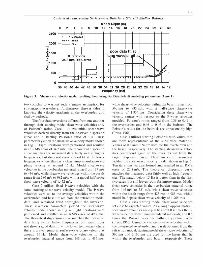
or Poisson’s ratios. Case 1 utilizes initial shear-wave

velocities derived directly from the observed dispersion

curve and a starting Poisson’s ratio of 0.4. These

parameters yielded the shear-wave velocity model shown

in Fig. 3. Eight iterations were performed and resulted

in an RMS error of 34.2 m/s. The theoretical dispersion

curve matches the measured data fairly well at higher

frequencies, but does not show a good fit at the lower

frequencies where there is a clear jump in surface-wave

phase velocity at around 16 Hz. Model shear-wave

velocities in the overburden material range from 137 m/s

to 436 m/s, while shear-wave velocities within the basalt

range from 380 m/s to 982 m/s, with a model half-space

shear-wave velocity of 1,452 m/s.

Case 2 utilizes fixed P-wave velocities with the

same starting shear-wave velocity model. The P-wave

velocities were set to the average velocities within the

overburden and basalt taken from the refraction model

data, and remained fixed throughout the inversion.

These inversion parameters yielded the shear-wave

velocity model shown in Fig. 4. Eight iterations were

performed and resulted in an RMS error of 49.9 m/s.

The theoretical dispersion curve matches the measured

data fairly well at higher frequencies, but, again, does

not show a good data fit at the lower frequencies where

there is a clear jump in surface-wave phase velocity at

around 16 Hz. Model shear-wave velocities in the

overburden material range from 146 m/s to 416 m/s,

while shear-wave velocities within the basalt range from

560 m/s to 935 m/s, with a half-space shear-wave

velocity of 1,954 m/s. Considering these shear-wave

velocity ranges with respect to the P-wave velocities

modeled, Poisson’s ratios ranged from 0.36 to 0.49 in

the overburden and 0.46 to 0.49 in the bedrock. The

Poisson’s ratios for the bedrock are unreasonably high

(Press, 1966).

Case 3 utilizes starting Poisson’s ratio values that

are more representative of the subsurface materials.

Values of 0.3 and 0.24 are used for the overburden and

the basalt, respectively. The starting shear-wave veloc-

ities correspond again to the ones derived from the

target dispersion curve. These inversion parameters

yielded the shear-wave velocity model shown in Fig. 5.

Ten iterations were performed and resulted in an RMS

error of 20.8 m/s. The theoretical dispersion curve

matches the measured data fairly well at high frequen-

cies. The match below 15 Hz is better than in the first

two cases, but still leaves room for improvement. Model

shear-wave velocities in the overburden material range

from 146 m/s to 531 m/s, while shear-wave velocities

within the basalt range from 423 m/s to 985 m/s, with a

model half-space shear-wave velocity of 1,965 m/s.

Case 4 uses starting model shear-wave velocities

set close to expected values. As a rough approximation,

shear-wave velocities are equal to about 0.4 times the P-

wave velocities within unconsolidated materials, and 0.6

times the P-wave velocities within crystalline rocks

(Press, 1966). Using the average P-wave velocities within

the interpreted overburden and basalt obtained from the

refraction model, starting model shear-wave velocities of

360 m/s and 2,160 m/s are used for the layers that lie

within the overburden and basalt, respectively. These

Figure 3. Shear-wave velocity model resulting from using SurfSeis default modeling parameters (Case 1).

119

Casto et al.: Interpreting Surface-wave Data for a Site with Shallow Bedrock

inversion parameters yielded the shear-wave velocity

model shown in Fig. 6. Ten iterations were performed

and resulted in an RMS error of 15.8 m/s, the lowest of

the four trials. The theoretical dispersion curve matches

the measured data very well at all sampled frequencies,

including where there is a clear jump in surface-wave

phase velocity at around 16 Hz. Model shear-wave

velocities in the overburden material range from 180 m/s

to 657 m/s, while shear-wave velocities within the basalt

range from 2,163 m/s to 2,175 m/s, with a model half-

space shear-wave velocity of 2,206 m/s.

Discussion of Field Data Outcomes

Figure 7 compares all inverted shear-wave velocity

models. Most models show a gentle increase in shear-

wave velocity beginning at depths between 7 and 10 m.

This corresponds well with the seismic refraction data,

and reasonably well with the lithology log that shows

clay overburden to a depth of 5.1 meters above

unweathered basalt. However, with the exception of

Case 4, which used the expected site conditions as the

starting model, all of the inversions failed to converge

Figure 5. Shear-wave velocity model resulting from using a starting Poisson’s ratio of 0.3 for the overburden and 0.24 for

the basalt (Case 3).

Figure 4. Shear-wave velocity model resulting from using fixed P-wave velocity constraints (Case 2). The P-wave

velocities for the overburden and the basalt were set to average velocities obtained from the seismic refraction

tomography model.

120

Journal of Environmental and Engineering Geophysics

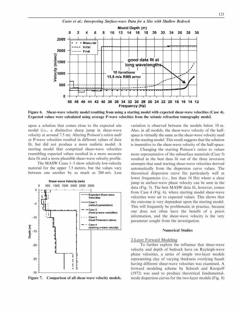
upon a solution that comes close to the expected site

model (i.e., a distinctive sharp jump in shear-wave

velocity at around 7.5 m). Altering Poisson’s ratios and/

or P-wave velocities resulted in different values of data

fit, but did not produce a more realistic model. A

starting model that comprised shear-wave velocities

resembling expected values resulted in a more accurate

data fit and a more plausible shear-wave velocity profile.

The MASW Cases 1–3 show relatively low-velocity

material for the upper 7.5 meters, but the values vary

between one another by as much as 260 m/s. Less

variation is observed between the models below 10 m.

Also, in all models, the shear-wave velocity of the half-

space is virtually the same as the shear-wave velocity used

in the starting model. This result suggests that the solution

is insensitive to the shear-wave velocity of the half-space.

Changing the starting Poisson’s ratios to values

more representative of the subsurface materials (Case 3)

resulted in the best data fit out of the three inversion

attempts that used starting shear-wave velocities derived

automatically from the dispersion curve values. The

theoretical dispersion curve fits particularly well at

lower frequencies (i.e., less than 16 Hz) where a clear

jump in surface-wave phase velocity can be seen in the

data (Fig. 5). The best MASW data fit, however, comes

from Case 4 (Fig. 6), where starting model shear-wave

velocities were set to expected values. This shows that

the outcome is very dependent upon the starting model.

This will frequently be problematic in practice, because

one does not often have the benefit of a priori

information, and the shear-wave velocity is the very

parameter sought from the investigation.

Numerical Studies

2-Layer Forward Modeling

To further explore the influence that shear-wave

velocity and depth of bedrock have on Rayleigh-wave

phase velocities, a series of simple two-layer models

representing clay of varying thickness overlying basalt

having different shear-wave velocities was examined. A

forward modeling scheme by Schwab and Knopoff

(1972) was used to produce theoretical fundamental-

mode dispersion curves for the two-layer models (Fig. 8)

Figure 6. Shear-wave velocity model resulting from using a starting model with expected shear-wave velocities (Case 4).

Expected values were calculated using average P-wave velocities from the seismic refraction tomography model.

Figure 7. Comparison of all shear-wave velocity models.

121

Casto et al.: Interpreting Surface-wave Data for a Site with Shallow Bedrock

having shear-wave velocities for basalt of 1,000 m/s,

2,000 m/s and 3,000 m/s, and overburden thicknesses of

2.5 m (Fig. 8, top), 5 m (Fig. 8, middle) and 10 m

(Fig. 8, bottom). The shear-wave velocity of the

overburden is constant for all models (284 m/s), and is

obtained from the observed surface-wave phase veloc-

ities at higher frequencies (i.e., the average velocity of

the asymptote observed in the overtone image). It

becomes clear in Fig. 8 that, for an overburden

thickness (i.e., depth to bedrock) greater than 5 m,

there is little observable change in surface-wave phase

velocity within the range of measured wavelengths

(maximum of 69 m). In other words, the wavelength at

which the fundamental-mode dispersion curves stop

exhibiting sensitivity to the overburden is larger than the

maximum wavelength sampled in our field data test. This

suggests why, given a fixed layer geometry, models having

a broad range of shear-wave velocities in the second layer

can all provide a good fit to the fundamental-mode

dispersion curves defined over the measured wavelengths.

Figure 8. Theoretical fundamental-mode dispersion curves for an overburden thickness of 2.5 m (top), 5 m (middle) and

10 m (bottom) and varying half-space shear-wave velocities.

122

Journal of Environmental and Engineering Geophysics

For a simple layered model, the low-frequency

limit of the fundamental-mode Rayleigh-wave phase

velocity will asymptotically approach a value slightly

less than the shear-wave velocity of the half-space (e.g.,

Xia and Xu, 2005). For the model that best represents

our field study, this would require data at frequencies

much lower than the observed limit of 13 Hz, perhaps

even less than 5 Hz (see Fig. 8). For the assumed phase

velocities, this corresponds to wavelengths greater than

400 m, which are far greater than the maximum

achieved with the survey equipment and geometry used.

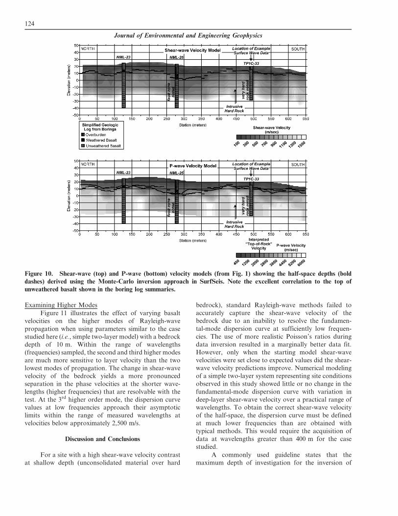
Solving for Depth

Figure 9 illustrates that surface-wave phase veloc-

ities for the same two-layer model are highly affected by

depth to bedrock. The curves in Fig. 9 represent the

theoretical fundamental-mode dispersion curves with

phase velocity as a function of wavelength for a fixed-

velocity half-space (VS 5 2,160 m/s, based upon the

modeled P-wave values) at depths ranging from 2.5 to

20 m. Within the range of the measured wavelengths

from the field data case (those less than 69 m), there is a

clear separation in phase velocities among the various

depth models.

To exploit the sensitivity of phase velocities to

layer thickness, an inversion of the field data was

performed in SurfSeis using a general Monte-Carlo

approach. The Monte-Carlo approach coded in SurfSeis

uses the overtone image directly to find the best-

matching solution through a random search. The

purpose of this test was to determine how effective the

MASW method can be in determining depth to bedrock

using a simple, fixed velocity structure. The shear-wave

velocities for the first layer and half-space were set to

284 m/s and 2,160 m/s, respectively, based upon the

data and the average modeled P-wave velocity displayed

in Fig. 1. Poisson’s ratios of 0.3 and 0.24 were fixed for

layer 1 and the half-space, respectively. Density was held

constant at 2.0 g/cm3. The inversion was directed to

match the overtone image, with data weighting propor-

tionate to the relative spectral amplitude at each

frequency. Figure 10 shows the shear-wave (top) and

P-wave (bottom) velocity models presented in Fig. 1

with the derived half-space depths overlain. There is

excellent correlation between the reported depth to the

top of unweathered basalt in the boring logs and the

calculated depths. This outcome demonstrates that a

combination of surface-wave studies utilizing funda-

mental-mode Rayleigh-wave dispersion with supplemen-

tary geological or geophysical data, such as borehole

lithologic data or seismic refraction data, would provide

a more accurate characterization of shallow bedrock

than would the use of fundamental-mode surface-wave

data alone.

Figure 9. Theoretical fundamental-mode dispersion curves for a range of overburden thicknesses (i.e., half-space depths)

and a half-space velocity of 2,160 m/s.

123

Casto et al.: Interpreting Surface-wave Data for a Site with Shallow Bedrock

Examining Higher Modes

Figure 11 illustrates the effect of varying basalt

velocities on the higher modes of Rayleigh-wave

propagation when using parameters similar to the case

studied here (i.e., simple two-layer model) with a bedrock

depth of 10 m. Within the range of wavelengths

(frequencies) sampled, the second and third higher modes

are much more sensitive to layer velocity than the two

lowest modes of propagation. The change in shear-wave

velocity of the bedrock yields a more pronounced

separation in the phase velocities at the shorter wave-

lengths (higher frequencies) that are resolvable with the

test. At the 3rd higher order mode, the dispersion curve

values at low frequencies approach their asymptotic

limits within the range of measured wavelengths at

velocities below approximately 2,500 m/s.

Discussion and Conclusions

For a site with a high shear-wave velocity contrast

at shallow depth (unconsolidated material over hard

bedrock), standard Rayleigh-wave methods failed to

accurately capture the shear-wave velocity of the

bedrock due to an inability to resolve the fundamen-

tal-mode dispersion curve at sufficiently low frequen-

cies. The use of more realistic Poisson’s ratios during

data inversion resulted in a marginally better data fit.

However, only when the starting model shear-wave

velocities were set close to expected values did the shear-

wave velocity predictions improve. Numerical modeling

of a simple two-layer system representing site conditions

observed in this study showed little or no change in the

fundamental-mode dispersion curve with variation in

deep-layer shear-wave velocity over a practical range of

wavelengths. To obtain the correct shear-wave velocity

of the half-space, the dispersion curve must be defined

at much lower frequencies than are obtained with

typical methods. This would require the acquisition of

data at wavelengths greater than 400 m for the case

studied.

A commonly used guideline states that the

maximum depth of investigation for the inversion of

Figure 10. Shear-wave (top) and P-wave (bottom) velocity models (from Fig. 1) showing the half-space depths (bold

dashes) derived using the Monte-Carlo inversion approach in SurfSeis. Note the excellent correlation to the top of

unweathered basalt shown in the boring log summaries.

124

Journal of Environmental and Engineering Geophysics

fundamental-mode Rayleigh waves is roughly equal to

half of the largest recorded wavelength. However, our

study of a high-velocity layer beneath a low-velocity

layer shows that the guideline does not ensure that

shear-wave velocity estimates will be accurate to this

depth. While it may be possible to predict the depth of

an interface up to the anticipated maximum depth,

based upon an observed increase in velocity gradient,

data at much lower frequencies (i.e., longer wavelengths)

may be required to resolve the shear-wave velocity

profile.

This study also demonstrated that the inversion

results are highly sensitive to choices for layer geometry

in the case of a high-velocity half-space beneath a low-

velocity layer. Numerical studies and tests on the field

data suggest that surface-wave methods can resolve

Figure 11. Theoretical dispersion curves for an overburden thicknesses of 10 m and varying half-space shear-wave

velocities for the 1st higher order (top), 2nd higher order (middle) and 3rd higher order (bottom) modes of Rayleigh-wave propagation.

125

Casto et al.: Interpreting Surface-wave Data for a Site with Shallow Bedrock

depth to bedrock in simple, layered geologies (e.g., soft

sediment over hard bedrock) when bulk velocities can be

inferred from supplementary data.

Practitioners of surface-wave techniques should be

aware of the constraint that the low-frequency limit

imposes upon resolution of both layer boundaries and

shear wave velocities at depth. The lack of low-

frequency data is common in practice. The lower

frequency, fundamental-mode data necessary to accu-

rately model shear-wave velocities to desired depths

might be acquired using longer geophone arrays with

stronger sources, or possibly by adding passive-source

techniques (Park et al., 2005; Park et al., 2007).

Dispersion data from higher modes of Rayleigh-

wave propagation, if available, may have been useful for

resolving depth and velocity of the high-velocity half-

space in the studied case, because the higher modes

theoretically reach the asymptotic high-velocity limits

within the range of recorded frequencies. Some relatively

recent published literature show that higher-mode phase

velocities of Rayleigh-waves appear to be more sensitive

to shear-wave velocities at greater depths for a given

frequency, and incorporating higher-mode dispersion

data in the inversion improves the accuracy of inversion

results (Beaty et al., 2002; Xia et al., 2003; Luo et al.,

2007; Supranata et al., 2007). The greatest benefit from

multiple-mode inversion techniques may be realized with

irregular subsurface velocity profiles (e.g., where stiffer

layers are underlain by softer layers) (Supranata et al.,

2007). Nevertheless, interpretation of higher-mode phase

velocities poses some challenges, as they are not always

easy to separate from the fundamental mode and possibly

from other scattered energy (e.g., Zhang and Chang,

2003). In practice, the occurrence of a high-velocity half-

space beneath lower-velocity materials or the presence of

stiff layers (Luke and Calderon-Macıas, 2007) is com-

monly encountered. Consequently, there is a real need by

practitioners for the availability of improved processing

and inversion techniques that incorporate higher-mode

dispersion data.

References

Beaty, K.S., Schmitt, D.R., and Sacchi, M., 2002, Simulated

annealing inversion of multimode Rayleigh wave dis-

persion curves for geological structure: Geophysical

Journal International, 151(2), 622–631.

Casto, D.W., Luke, B., Calderon-Macıas, C., and Kaufmann,

R., 2008, Considerations for interpreting surface wave

data in sites with shallow bedrock: in Expanded

Abstracts: 21st Annual Symposium on the Applications

of Geophysics to Engineering and Environmental

Problems (SAGEEP), 13 pp.

Ivanov, J., Miller, R.D., Lacombe, P., Johnson, C.D., and

Lane, J.W. Jr., 2006, Delineating a shallow fault zone

and dipping bedrock strata using multichannel analysis

of surface waves with a landstreamer: Geophysics, 71(5),

A39–A42.

Kansas Geological Survey, 2006, SurfSeis v2.0 MASW:

Kansas Geological Survey, Lawrence, Kansas.

Luke, B., and Calderon-Macıas, C., 2007, Inversion of seismic

surface wave data to resolve complex profiles: Journal

of Geotechnical and Geoenvironmental Engineering,

133(2), 155–165.

Luo, Y., Xia, J., Liu, J., Liu, Q., and Xu, S., 2007, Joint

inversion of high-frequency surface waves with funda-

mental and higher modes: Journal of Applied Geophys-

ics, 62(4), 375–384.

Miller, R.D., Xia, J., Park, C.B., and Ivanov, J., 1999,

Multichannel analysis of surface waves to map bedrock:

in The Leading Edge, 18(12), 1392–1396.

Oyo Corporation, 2006, SeismImager/2D, v3.2: Oyo Corpo-

ration, Japan.

Park, C.B., Miller, R.D., and Xia, J., 1998, Imaging dispersion

curves of surface waves on multi-channel record: in

Expanded Abstracts: 68th Annual International Meet-

ing, Society of Exploration Geophysics, 1377–1380.

Park, C.B., Miller, R.D., Ryden, N., Xia, J., and Ivanov, J.,

2005, Combined use of active and passive surface waves:

Journal of Environmental and Engineering Geophysics,

10(3), 323–334.

Park, C.B., Miller, R.D., Xia, J., and Ivanov, J., 2007,

Multichannel analysis of surface waves (MASW)—

active and passive methods: in The Leading Edge,

26(1), 60–64.

Press, F., 1966, Seismic velocities: in Handbook of physical

constants, revised edition, Clark, S.P., Jr. (ed.), Geolog-

ical Society of America Memoir, 97, 97–173.

Schwab, F.A., and Knopoff, L., 1972, Fast surface wave and

free mode computations: in Methods in Computational

Physics, Bolt, B.A. (ed.), Academic Press, 87–180.

Song, Y.Y., Castagna, J.P., Black, R.A., and Knapp, R.W.,

1989, Sensitivity of near-surface shear-wave velocity

determination from Rayleigh and Love waves: in

Expanded Abstracts: 59th Annual International Meet-

ing, Society of Exploration Geophysics, 509–512.

Stokoe, K.H. II, Wright, S.G., Bay, J.A., and Roesset, J.M.,

1994, Characterization of geotechnical sites by SASW

method: in Geophysical characterization of sites,

Woods, R.D. (ed.), Oxford & IBH Publishing Company,

New Delhi, India, 15–25.

Supranata, Y.E., Kalinski, M.E., and Ye, Q., 2007, Improving

the uniqueness of surface wave inversion using multiple-

mode dispersion data: International Journal of Geome-

chanics, 7(5), 333–343.

Xia, J., Miller, R.D., and Park, C.B., 1999, Estimation of near-

surface shear-wave velocity by inversion of Rayleigh

waves: Geophysics, 64, 691–700.

Xia, J., Miller, R.D., Park, C.B., Hunter, J.A., Harris, J.B.,

and Ivanov, J., 2002, Comparing shear-wave velocity

profiles inverted from multichannel surface wave with

borehole measurements: Soil Dynamics and Earthquake

Engineering, 22, 181–190.

126

Journal of Environmental and Engineering Geophysics

Xia, J., Miller, R.D., Park, C.B., and Tian, G., 2003, Inversion of

high frequency surface waves with fundamental and higher

modes: Journal of Applied Geophysics, 52(1), 45–57.

Xia, J., and Xu, Y., 2005, Discussion on some practical

equations with implications to high-frequency surface-

wave techniques: in Expanded Abstracts: 18th Annual

Symposium on the Applications of Geophysics to

Engineering and Environmental Problems (SAGEEP),

1089–1104.

Zhang, S.X., and Chan, L.S., 2003, Possible effects of

misidentified mode number on Rayleigh wave inversion:

Journal of Applied Geophysics, 53(1), 17–29.

127

Casto et al.: Interpreting Surface-wave Data for a Site with Shallow Bedrock