interpreting multiple correspondence analysis as a...

Marketing Letters 3:3, (1992): 259-272 © 1992 Kluwer Academic Publishers, Manufactured in the Netherlands.

Interpreting Multiple Correspondence Analysis as a Multidimensional Scaling Method

DONNA L. HOFFMAN* S«hool of Management, University of Texas at Dallas, JO 5.1, Riehardson, TX 75083-0688, (2t4) 690-2545, E-mail: [email protected]

JAN DE LEEUW Department of Mathematics, 7228 MSB, UCLA, Los Angeles CA 90024-1555, (213) 825-9550, E- mail: [email protected]

Key words: Graphical Representation of Categorical Data, Homogeneity, Nonlinear Multivariate Analysis

[January 1992]

Abstract

We formulate multiple correspondence analysis (MCA) as a nonlinear multivariate analysis method that integrates ideas from multidimensional scaling. MCA is introduced as a graphical technique that minimizes distances between connecting points in a graph plot. We use this geometrical approach to show how questions posed of categorical marketing research data may be answered with MCA in terms of closeness. We introduce two new displays, the star plot and line plot, which help illustrate the primary geometric features of MCA and enhance interpretation. Out approach, which extends Gifi (1981, 1990), emphasizes easy-to-interpret and managerially relevant MCA maps.

Multiple correspondence analysis (MCA) is weil on its way to becoming a popular tool in marketing research (Hoffman & Franke, 1986). For example, Green, Krie- ger, and Carroll (1987) use MCA to analyze the relationship between consumers' choice profile predictions from a conjoint task and consumer demographic characteristics. In a similar vein, Kaciak and Louviere (1990) illustrate how MCA may be used to analyze data from discrete choice experiments. Carroll and Green (1988) apply individual differences MDS to normalized Burt matrices (a principal data matrix in MCA) to determine the relationship between consumer demograph- ics and automobile characteristics with respect to number of cars in the house- hold. More recently, Valette-Florence and Rapacchi (1991) perform an MCA on the attributes-consequences-values matrix derived from a laddering task to construct a product positioning map and Hoffman and Batra (1991) apply MCA to study the association between television program types and audience viewing be- haviors.

*The authors thank J. Douglas Carroll, Don Lehmann, Donald Morrison, and two anonymous reviewers for their helpful comments on a previous version of this manuscript.

260 DONNA L. HOFFMAN AND JAN DE LEEUW

We focus in this paper on the interpretation of MCA maps. The fundamental issue concerns the appropriate way to represent both the objects corresponding with the rows and variables corresponding with the columns of the data matrix in the same map. This problem has become increasingly more important because the three major statistical packages now have MCA modules in which the choice of scaling of row and column coordinates is left largely to the user (BMDP 1988; SAS Institute Inc. 1988; SPSS Inc. 1989). In addition, the variety of commercially available PC-based programs offer numerous options but little guidance to the user (BMDP 1988; Greenacre 1986; Nishisato and Nishisato 1986; SAS Institute Inc. 1988; Smith, 1988; see also Hoffman (1991) for a review).

We present a geometrical approach to MCA that provides for enhanced representation and interpretation of MCA maps. Our work extends the treatment in Girl (1981, 1990) by placing increased emphasis on the geometry. Two new in- terpretive maps are introduced: star plots and the variable line plot. MCA is de- veloped as an MDS method that minimizes the distances between connecting points in a graph plot. We feel that these additional geometric properties make MCA easier to understand.

1. Correspondence analysis as a model

What is multiple correspondence analysis? The French literature (see, for example, Benzécri et al. 1973) discusses it in the context of metric multidimensional scaling suitable for frequency matrices, contingency tables, or cross-tables. Oth- ers formulate MCA as factorial analysis of qualitative data using scale analysis (e.g., Nishisato 1980) or principal component analysis (e.g., de Leeuw 1973) per- spectives.

We formulate MCA in terms of connecting objects, brands say, with all the variable categories they are in and use a least-squares loss function as the rule to do this. Then, interpretation sterns not from terms of chi-square distance or profiles (cf. Hoffman and Franke 1986), but rather, follows from le principe bary- centrique, the centroid principle, which says that brands close to each other are similar to each other. Our approach thus emphasizes the geometrical aspects of multiple correspondence analysis.

2. M C A as an MDS method

The concept of homogeneity serves as the basis for our development of multiple correspondence analysis. Homogeneity refers to the extent to which different variables measure the same characteristic or characteristics (Girl 1981, 1990). Ho- mogeneity thus specifies a type of similarity. There are different measures of homogeneity and different approaches to find mäps; the particular choice of loss function defines the former and the specific algorithm employed determines the latter.

INTERPRETING MULTIPLE CORRESPONDENCE ANALYS1S 261

Suppose we think of a rectangular data matrix as a multivariable representat ion (i.e., as a joint map of the brands and the variable categories) in two-dimensional Euclidean space. The map will be more appealing if brands are close to the categories of the variables that they occur in. This is the basic premise of multiple correspondence analysis. By the triangle inequality this implies that brands with similar profiles (i.e., brands that are offen in the same categories) will be close, and categories containing roughly the same brands will be close as well. We now formalize these ideas by defining a suitable loss function to be minimized.

2.1. Maximizing variable homogeneity

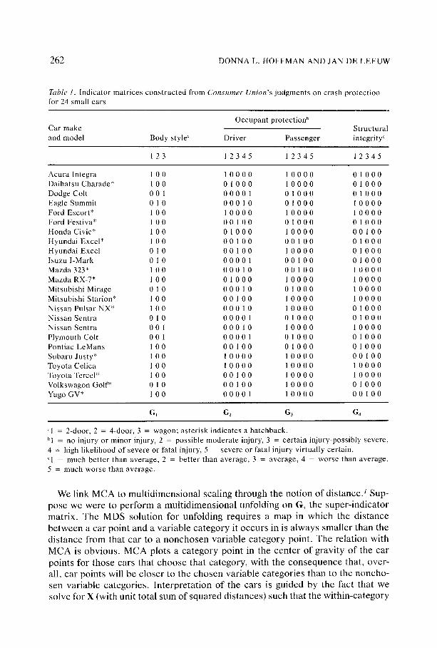
Let the data be m categorical variables on n objects, with the jth variable taking on k i different values, its categories. We code the variables using indicator matrices to allow for easy expression in matrix notation. An indicator matri× is a binary matrix (exactly one element equal to one in each row) that indicates the category an object is in for a particular variable. Thus, if variable j has kj categories, then Gj, the indicator matrix for this variable is n × k~ and each row of Gj sums to one. More specifically, consider the example of G = [Gj] . . . IG,,] in table 1, with m = 4, n = 24, kl = 3, k2 = 5, k3 = 3, and k4 = 3. Here, the objects are 24 small cars that Consumers Union judged by degree of crash protect ion (Consumers Union, 1989). These judgments are based on Consumers Union's analysis of National Highway Traffic Safety Administration crash-test data. The two occupant protection variables indicate how well the car protected a driver dummy and a passenger dummy during crash tests. Structural integrity indicates how weil the passenger compar tment held up to the forces of a crash; bet ter performance is associated with a greater chance of avoiding injuries other than those caused by the imme- diate forces of a crash. The remaining categorical variable indicates car body style.

The purpose of multiple correspondence analysis is to construct a jo in t map of cars and variable categories in such a way that a car is relatively close to a category it is in, and relatively far from the categories is it not in. By the triangle inequality, this implies that cars mostly occurring in the same categories rend to be close, while categories sharing mostly the same cars tend to be close, as well. The extent to which a particular scaling X of the cars and particular scalings Y« of the categories, satisfy this is quantified by the loss of homogeneity, a least squares loss function:

~r(X;Y, ..... Ym) = Zj S S Q ( X - G f f ) (l)

where SSQ(.) is shorthand for the sum of squares of the elements of a matrix or vector. The loss function in (1), giving the sum of squares of the distances between cars and the categories they occur in, measures departure from perfect homogeneity or similarity. Quite simply, muRiple correspondence analysis produces the map with the smallest possible loss (Girl 1981; 1990).

262 D O N N A L. H O F F M A N AND JAN DE LEEUV~

Table I. lndicator matrices constructed from C o n s u m e r Union's judgments on crash protection for 24 small cars

Occupant protection b Car make Structural and model Body style" Driver Passenger integrity c

1 2 3 1 2 3 4 5 1 2 3 4 5 1 2 3 4 5

A c u r a l n t e g r a 1 0 0 1 0 0 0 0 1 0 0 0 0 0 1 0 0 0 Daiha t suCharade* 1 0 0 0 1 0 0 0 1 0 0 0 0 0 1 0 0 0 Dodge Colt 0 0 1 0 0 0 0 1 0 1 0 0 0 0 1 0 0 0 Eag leSummi t 0 1 0 0 0 0 1 0 0 1 0 0 0 1 0 0 0 0 Ford Escort* 1 0 0 1 0 0 0 0 1 0 0 0 0 1 0 0 0 0 FordFes t iva* 1 0 0 0 0 1 0 0 0 1 0 0 0 0 1 0 0 0 HondaCiv ic* 1 0 0 0 1 0 0 0 1 0 0 0 0 0 0 1 0 0 Hyunda iExce l* 1 0 0 0 0 1 0 0 0 0 1 0 0 0 1 0 0 0 Hyunda iExce l 0 1 0 0 0 1 0 0 1 0 0 0 0 0 1 0 0 0 I s u z u I - M a r k 0 1 0 0 0 0 0 1 0 0 1 0 0 0 1 0 0 0 Mazda323* 1 0 0 0 0 0 1 0 0 0 1 0 0 1 0 0 0 0 MazdaRX-7* 1 0 0 0 1 0 0 0 1 0 0 0 0 1 0 0 0 0 MitsubishiMirage 0 1 0 0 0 0 1 0 0 1 0 0 0 1 0 0 0 0 Mitsubishi Starion* I 0 0 0 0 1 0 0 1 0 0 0 0 I 0 0 0 0 N i s s a n P u l s a r N X * 1 0 0 0 0 0 1 0 1 0 0 0 0 0 1 0 0 0 N i s s a n S e n t r a 0 1 0 0 0 0 0 1 0 1 0 0 0 0 ! 0 0 0 N i s s a n S e n t r a 0 0 1 0 0 0 1 0 1 0 0 0 0 1 0 0 0 0 P lymouthCol t 0 0 1 0 0 0 0 1 0 1 0 0 0 0 1 0 0 0 Pon t i a cLeMans 1 0 0 0 0 1 0 0 0 1 0 0 0 0 1 0 0 0 S u b a r u J u s t y * 1 0 0 1 0 0 0 0 1 0 0 0 0 0 0 1 0 0 Toyota Celica 1 O0 1 0 0 0 0 1 0 0 0 0 1 0 0 0 0 Toyota Tercel* I O0 O01 O0 1 0 0 0 0 1 0 0 0 0 VolkswagonGolf* 0 1 0 O01 O0 1 0 0 0 0 0 1 0 0 0 Yugo GV* I O0 0 0 0 0 1 1 0 0 0 0 O01 O0

Gj G2 Gj G 4

"l = 2-door, 2 - 4-door, 3 = wagon; asterisk indicates a hatchback. bi = no injury or minor injury, 2 = possible moderate injury, 3 = certain injury-possibly severe, 4 = high likelihood of severe or fatal injury, 5 severe or fatal injury virtually certain. ~1 = rauch better than average, 2 = bet tet than average, 3 = average, 4 = worse than average,

5 = much worse than average.

We link MCA to multidimensional scaling through the notion of d i s tanceJ Sup- pose we were to per form a multidimensional unfolding on G, the super-indicator matrix. The MDS solution for unfolding requires a map in which the distance between a car point and a variable category it occurs in is always smaller than the distance f rom that car to a nonchosen variable category point. The relation with MCA is obvious. MCA plots a category point in the center of gravity of the car points for those cars that choose that category, with the consequence that, over- all, car points will be closer to the chosen variable categories than to the nonchosen variable categories. Interpretat ion of the cars is guided by the fact that we solve for X (with unit total sum of squared distances) such that the within-category

INTERPRETING MULTIPLE CORRESPONDENCE ANALYSIS 263

squared Euclidean distances are as small as possible (or, equivalently, that the between-category squared Euclidean distances are as large as possible). Note that this amounts to the same thing as performing multidimensional scaling on a similarity matrix S = {su} with s•= 1 if there is a match between the similarity of car i and variable category j, and 0 otherwise. The primary difference between MCA and MDS is that the MCA solution is obtained at the expense of stronger normalization conditions and a metric interpretation of the data. However , MDS methods for unfolding make weaker assumptions, but also tend to produce degen- erate solutions. 2

The MCA algorithm, implemented in the SPSS-X program CATEGORIES (SPSS Inc. 1989), is exceedingly simple and relies on alternating least squares (or, equivalently, reciprocal averaging (Hirschfeld 1935; Horst 1935)). The optimal variable category coordinates are computed as the averages or centroids of the (optimal) coordinates of the cars in that category:

v r : I ) # % ' x (3)

with Gj defined as above, and Dj = G/Gj the k~ x kj diagonal matrix containing the univariate marginals of variable j. Similarly, the optimal car coordinates are the centroids of the (optimal) coordinates of the categories containing that car:

X = m 1ZiG«Y j (4)

3. Multiple correspondence analysis of the car data

3.1. The graph plot

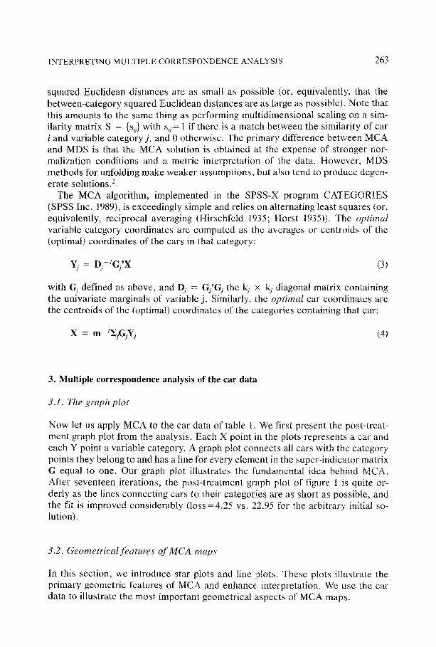
Now let us apply MCA to the car data of table 1. We first present the post-treatment graph plot from the analysis. Each X point in the plots represents a car and each Y point a variable category. A graph plot connects all cars with the category points they belong to and has a line for every element in the super-indicator matrix G equal to one. Out graph plot illustrates the fundamental idea behind MCA. After seventeen iterations, the post- treatment graph plot of figure 1 is quite or- derly as the lines connecting cars to their categories are as short as possible, and the fit is improved considerably (loss = 4.25 vs. 22.95 for the arbitrary initial solution).

3.2. Geometrical features of MCA maps

In this section, we introduce star plots and line plots. These plots illustrate the primary geometric features of MCA and enhance interpretation. We use the car data to illustrate the most important geometrical aspects of MCA maps.


X

X

Figure 1. Post-Treatment Graph Plot

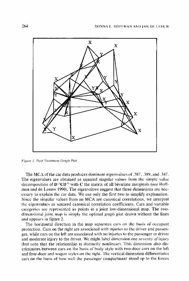
The MCA of the car data produces dominant eigenvalues of .587, .389, and .347. The eigenvalues are obtained as squared singular values from the simple value decomposit ion of D-'/-'CD -'/-' with C the matrix of all bivariate marginals (see Hoff- man and de Leeuw 1990). The eigenvalues suggest that three dimensions are nec- essary to explain the car data. We use only the first two to simplify explanation. Since the singular values from an MCA are canonical correlations, we interpret the eigenvalues as squared canonical correlation coefficients. Cars and variable categories are represented as points in a joint low-dimensional map. The two- dimensional joint map is simply the optimal graph plot drawn without the lines and appears in figure 2.

The horizontal direction in the map separates cars on the basis of occupant protection. Cars on the right are associated with injuries to the driver and passenger, while cars on the left are associated with no injuries to the passenger or driver and moderate injury to the driver. We might label dimension one severity of in jury (but note that the relationship is distinctly nonlinear). This dimension also discriminates between cars on the basis of body style with two-door cars on the left and four-door and wagon styles on the right. The vertical dimension differentiates cars on the basis of how well the passenger compar tment stood up to the forces


¢~ 0.4 Œ

o

Œ o E "1= 0.2

0 • 0 "

-0.2

-0.4 - 0 . 4

Figure 2. Joint Map

[ ]

mazda 323 [] ser inj dr eagle summit

. mitsubishi mirage

mitsubishi starion [] nissan centra toyota tercel a rauch better

ford escort nissan pulsar nx toyota celica [] cer7 injpas

[ ] [ ] .

mazda rx-7 hyundai excel • 4 - d o o r [] [] [] hyundai excel [ ] ~ c e r t inj dr [] v o l k s w a g e n .¢lo, lf .

• . 7..aoor . " m o a mjpos no in jdr n o m j p a s [] isuzu J-marK

~' ford festivai better == m o d inj dr acura integnpontia c lemans «wagon

u el

daithatsu charade []

subaru j us t y

[ ] [ ] average honda eivic

[ ] yugo gv

| !

- 0 . 2 0 .0

œ

nissan centra m

fa t ißi dr [ ]

p lymouth col t do¢lge coR

0 .2 0 .4

d i m e n s i o n I

of a crash. Structural integrity is best for cars at the top of the map and worsens (to average) as we move to the |ower left.

The distance between two car points is related to the homogeneity (i.e., the similarity) of their profiles, or more generally, their response-patterns/Cars with identical patterns are plotted as identical points. This is iIlustrated in figure 2 for, among others, Plymouth Colt and Dodge Colt in the lower right and Eagle Summit and Mitsubishi Mirage in the upper right, which have identical profiles in G. Two very similar cars are the two Hyundai Excels near the center right of figure 2.

Another feature of the map is indicated by the positions, for example, of the categories average structural integrity and wagon styte. These point locations indicate that a category point with low marginal frequency will be plotted towards the edge of the map, while a category with high marginal frequency (two-door style, no injury to passenger, and better structural integrity) wiil be plotted nearer to the origin of map. As a corollary, cars with response patterns similar to the average response pattern will be piotted more towards the origin (the two-door and four-door Hyundai Excels and Volkswagon GolD, while cars with unique patterns (for example, Mazda 323 and Yugo GV) appear near the edges.

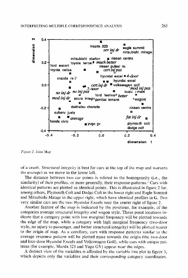
A distinct view of the variables is afforded by the variable line plot in figure 3, which depicts only the variables and their corresponding category coordinates.


N

c-

O

c -

o

E

0.3

0.2

0,1

0.0

-0.1

-0.2

-0.3 -0 .3

A ;TZ ,njor, much better integrity/ ~

/ ~ e e r t a i n injury passenger ~ - d o o r

no injury t ~ o ~ , , , ..... \ N ~ d r i v e r ......--.~11~"~ drlve'r .... '~." \

r /no injury k moderate injury [ / ' - better integrity / Dassenaer ~.Passe~er~l " / . . \ wagon

moderate injury \ driver/ ~ ,

fatal injury average integrity d river

I I I I I

-0.2 -0.1 0.0 0.1 0.2 0.3 dimension 1

Figure 3. Line Plot

Table 2. The discrimination measures per variable per dimension

Variable Dimension

One Two

Body Style .621 ,082 Driver Protection .714 .750 Passenger Protection ,642 .043 Structural Integrity .373 .681

h .587 .389

The line plot illustrates the spread of the category points for each variable. A variable discriminates bet ter to the extent that its category points are further apart. The line plot thus show how well each variable discriminates, as visualized by the sum of the squared distances between the category points for a variable and the origin. Discrimination measures are quantified as the squared correlations between the car coordinates X and the optimally t ransformed variables, G;Yj, and are interpreted as squared factor loadings. We show them in table 2. The larger

[NTERPRETING MULTIPLE CORRESPONDENCE ANALYSIS 267

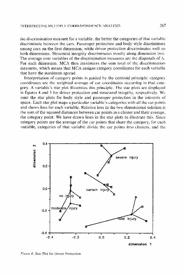
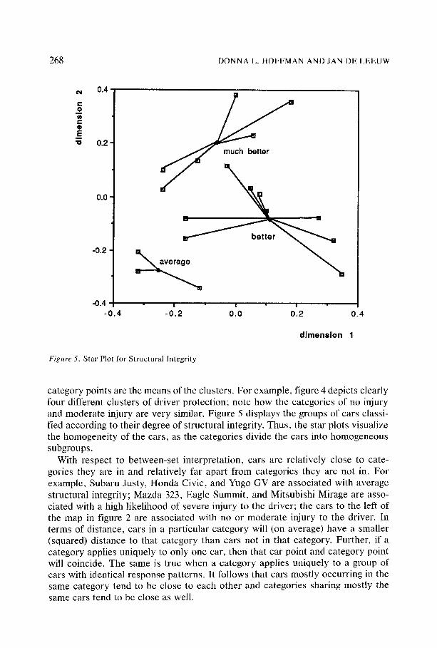
the discrimination measure for a variable, the better the categories of that variable discriminate between the cars. Passenger protection and body style discriminate among cars on the first dimension, while driver protection discriminates well on both dimensions. Structural integrity discriminates mostly along dimension two. The average over variables of the discrimination measures are the diagonals of A. For each dimension, MCA thus ma×imizes the sum total of the discrimination measures, which means that MCA assigns category coordinates for each variable that have the maximum spread.

Interpretation of category points is guided by the centroid principle: category coordinates are the weighted average of car coordinates occurring in that category. A variable's star plot illustrates this principle. The star plots are displayed in figures 4 and 5 for driver protection and structural integrity, respectively. We omit the star plots for body style and passenger protection in the interests of space. Each star plot maps a particular variable's categories with all the car points and shows loss for each variable. Relative loss in the two-dimensional solution is the sum of the squared distances between car points in a cluster and their average, the category point. We have drawn lines in the star plots to illustrate this. Since category points are the average of the car points that share the category, for each variable, categories of that variable divide the car points into clusters, and the

Œ

0

t -

O

E m "O

0.4

0.2

0.0

ù0.2 m ode~e//inju r'~y

-0.4 !

-0.4 -0.2

I ~ e injury

0.0 0.2 0.4 dimension 1

Fi~,m'e 4. Star Plot for Driver Protection


Œ 0 œ c- O E

"0

0.4

0.2'

0.0

-0.2

-0.4 I

-0 .4 -0=.2 010 0.2

dimension

Figure 5. Star Plot for Structural Integrity

0.4

1

category points are the means of the clusters. For example, figure 4 depicts clearly four different clusters of driver protection; note how the categories of no injury and moderate injury are very similar. Figure 5 displays the groups of cars classi- fied according to their degree of structural integrity. Thus, the star plots visualize the homogenei ty of the cars, as the categories divide the cars into homogeneous subgroups.

With respect to between-set interpretation, cars are relatively close to categories they are in and relatively far apart from categories they are not in. For example, Subaru Justy, Hondä Civic, and Yugo GV are associated with average structural integrity; Mazda 323, Eagle Summit, and Mitsubishi Mirage are associated with a high likelihood of severe injury to the driver; the cars to the left of the map in figure 2 are associated with no or moderate injury to the driver. In terms of distance, cars in a particular category will (on average) have a smaller (squared) distance to that category than cars not in that category. Further, if a category applies uniquely to only one car, then that car point and category point will coincide. The same is true when a category applies uniquely to a group of cars with identical response patterns. It follows that cars mostly occurring in the same category tend to be close to each other and categories sharing mostly the same cars tend to be close as weil.


4. Discussion

4.1. Graphical representation

In our framework, distances corresponding to ls in G must be small (compared to distances corresponding to 0s), but this requirement alone is not sufficient to produce a map, since the trivial solution satisfies it. Hence, we need a normalization. A natural normalization would be to examine all the distances and simply minimize the between-set distances (i.e., the sum of squares) keeping all other distances fixed. Unfortunately, this always leads to a one-dimensional solution. Thus, we require something stricter, so we impose dimension orthogonality and normalization constraints. Which way we choose to normalize (i.e., normalize the objects X and leave the variables Y: free, or the reverse) is immaterial geometri- cally, since the problem is formulated in a joint space. However, choice of normalization affects interpretation. Therefore, the researcher must make a choice with substantive considerations the guide.

The centroid principle defines graphical representation and interpretation of the MCA map. Its rationale lies in the inherent asymmetry of multivariate data. Al- most all of the applications of MCA that we have seen, and consequently almost all interpretations, are inherently asymmetric since multivariate data are by definition row or column conditional. In other words, in the context of a specific marketing analysis, we treat rows and columns differently since each represents distinct entities we wish to characterize graphically.

Consider the matrix with rows defined by a set of brands and columns a set of attributes describing the brands. Row conditionality implies that we primarily wish to emphasize the brands and scale them such that in the map, brands are closer together to the extent that they are more similar with respect to the attributes. This suggests that it is logical to think of ordering brands by attributes. Columns, i.e., attribute categories, are the center of gravity of the brands. Prac- tically speaking, choosing the normalization implied by row conditional data means that brands will be equally spread in all directions in the map, with attribute category points indicating the weighted averages of the brands in that category. In other words, brands are sorted into their respective categories of an attribute. This leads, as in our car data example, to a single map for the brands and a set of star plots for each separate variable.

Thus, for row conditional data, we normalize the set of object coordinates X and leave the variable category coordinates y: free. We denote this Case 1. This means that the variable categories Y: are found by the centroid principle. In this case, the optimal scaling of a variable category (equation 3) satisfy Y~'DjYj = X'GjD:-~G/X and thus Y'DY = mX'P.X = mA, with P. the average of the GjDiIGj. Quite simply, in words, a variable category coordinate is the centroid of the coordinates of the objects in that category. Gift (1981, 1990) calls this the first centroid principle.

Now consider that rows are consumers and columns are a set of categorical variables which the consumers have evaluated. Column conditionality implies


that we primarily wish to represent the variable categories as points in a map and scale them such that variables close together are more similar with respect to the consumers in the matrix. This normalization of MCA orders variables by these individuals. Then, we obtain a single map for all the variable categories and, if desired, a set of star plots for each individual with categories of all variables in the plots. Now, variable categories are equally dispersed in all directions and the centroid interpretation applies to the individuals. As applications in this context often involve very large numbers of individuals, we typically omit the star plots and focus research attention on the graph plot of variables only. Accordingly, we normalize the set of variables and teave the objects free. In this Case H, the X are found by the centroid principle and the optimal scaling of the objects (equation 4) satisfies X'X = m-1Y'DYA = A. In words, the optimal coordinate of an object is the centroid of the coordinates of the variable categories the object occurs in. Girl (1981, 1990) calls this the second centroid principle.

It will almost always be the case that primary focus is on either the rows or the columns, but not both equally. However, we may normalize according to Case III, in which both the objects and the variable categories are normalized. Some- times referred to as the French scaling, this option treats rows and columns sym- metrically and drops the centroid principle. Within-set relations are interpretable as chi-square distances, 4 but no between-set interpretation is possible. For example, Greenacre (1989) prefers to normalize according to Case III (symmetri- cally scaling both sets of points in principal coordinates) and emphasize the within-set chi square distances at the expense of any between-set interpretation. Carroll, Green, and Scharfer (1986) recommend a variant of Case III, the so-called CGS scaling, which they argue provides for interpretation of all distances (but see Greenacre (1989) for a dissenting view). What should be clear from out discussion, however, is that the aims of the investigation guide the researcher's choice of representation and interpretation.

4.2. Concluding remark

Our geometric approach suggests that MCA is fruitfully thought of as a nonlinear multivariate analysis method that seeks to minimize the distance between lines connecting objects with all the categories they are in, rather than as a method to represent chi-square distances. Out bias suggests that simple CA may be more naturally thought of as a special case of MCA with the number of variables equal to two than as a method to approximate within-set chi-square distance. Finally, we believe that if marketing researchers consider the relationship between correspondence analysis and multidimensional scaling through MCA (and the graph plot), rather than through CA (and the chi-square distance metric), they should have little difficulty interpreting the results from this powerful multivariate meth- odology.

~NTERPRETING MULTIPLE CORRESPONDENCE ANALYSIS 271

Notes

1. We can also reformulate the MCA problem in discriminant analysis or ANOVA terms. This development connects MCA to classical multivariate analysis. See Hoffman and de Leeuw (1990) for a fulter treatment.

2. But see DeSarbo and Rao (1984, 1986) for a multidimensional unfolding solution, incorporating reparameterization, which avoids the degeneracy problem. DeSarbo and Hoffinan (1986, 1987) extend the model to binary data and compare the solutions with correspondence analysis.

3. Note that the reverse will not necessarily be true. Two car points that are dose together in a map of the first two-dimensions may be far apart in higher dimensionalities.

4. The "chi-square" distance between two row points, say, is equal to the weighted sum of squared differences between row "profi le" values, with weights equal to the inverse of the relative fre- quencies of the columns. A similar definition holds for column points. These within-set distances are denoted chi-square because if the data a r e a contingency table, then the numerator creates squared differences between conditional row probabilities (the profilesL while the de- nominator weights the squared differences by inverse relative column marginals; thus. as Novak and Hoffman (1990) show, distances can be interpreted in terms of a) standardized residuals (components of chi-square), b) O - E~/E ~, observed minus expected counts under the log-!inear model of independence as a proportion of expected counts under independence, and c) "profiles" (conditional probabilities).

References

Benzécri, Jean-Paul, et al. (1973). L'Analyse des Données. (2 vols.) Paris: Dunod. BMDP Statistical Software, Inc. (1988). CA: Correspondence Analysis. Technical Report No. 87.

Los Angeles, CA. Carroll, J. Douglas, and Paul E. Green. (1988). "An INDSCAL-Based Approach to Muttiple Cor-

respondence Analysis," Journal of Marketing Research 25 (May), I93-203. Carroll, J. Douglas, Paul E. Green, and Catherine M. Scharfer. (1986). "Interpoint distance Com-

parisons in Correspondence Analysis," Journal of Marketing Research 23 (August), 271-280. Consumers Union. (1989). "Which Cars Do Bet te t in a Crash?" Consumer Reports April, 208-

211. de Leeuw, Jan. (1973). Canonical Analysis of Categorical Data. Unpublished doctoral disserta-

tion, Psychological Institute, University of Leiden, The Netherlands. Reissued DSWO-Press, Leiden, 1984.

DeSarbo, Wayne S., and Donna L. Hoffman. (1986). "Simple and Weighted Unfolding Threshold Models for the Spatial Representation of Binary Choice Data" Applied Psychotogical Measure- ment 10 (September), 247-264.

DeSarbo, Wayne S., and Donna L. Hoffman. (1987). "Constructing MDS Joint Spaces from Binary Choice Data. A New Multidimensional Unfolding Model for Marketing Research," Jonrnal oj Marketing Research 24 (February), 40-54.

DeSarbo, Wayne S., and Vithala Rao. (1984). "GENFOLD2: A Set of Models and Algorithms for the GENeral unFOLDing Analysis of Preference/Dominance Data ," Journal ofClassification l (Winter), 147-186.

DeSarbo, Wayne S., and Vithala Rao. (1986). "A Constrained Unfolding Model for Product Posi- tioning Analysis," Marketing Science 5 (Winter), 1-19.

Girl, Albert. (1981). Non-linear Muttivariate Analysis. Leiden: Department of Data Theory. Girl, Albert. (1990). Non-linear Multivariate Analysis. New York: Wiley. Green, Paul E., Abba M. Krieger, and J. Douglas Carroll. (1987). "Multidimensional Scaling: A

Complementary Approach," Joarnal ofAdvertising Research October/November, 21-27.


Greenacre, Michael J. (1986). "SIMCA: A Program to Perform Simple Correspondence Analysis," American Statistician 51,230-231.

Greenacre, Michael J. (1989). "The Carroll-Green Scharfer Scaling in Correspondence Analysis: A Theoretical and Empirical Appraisal," Journal of Marketing Research 26 (August), 358-365.

Hirschfeld, H. O. (1935). "A Connection between Correlation and Contingency," Proceedings oJ the Cambridge Philosophical Society 31 (October), 520-524.

Hoffman, Donna L. (1991). "Review of Four Correspondence Analysis Programs for the IBM PC," American Statistician 45 (4), November, 305-311.

Hoffman, Donna L., and Rajeev Batra. (1991). "Viewer Response to Programs: Dimensionality and Concurrent Behavior," Journal ofAdvertising Research August/September, 46-56.

Hoffman, Donna L., and Jan de Leeuw. (1990). "Geometrical Aspects of Multiple Correspondence Analysis: Implications for the Coordinate Scaling Debate," UCLA Statistics Series, No. 49.

Hoffman, Donna L., and George R. Franke. (1986). "Correspondence Analysis: Graphical Rep- resentation of Categorical Data in Marketing Research," Journal of Marketing Research 23 (Au- gust), 213-227.

Horst, Paul. (1935). "Measuring Complex Attitudes," Journal ofSocial Psychology 6 (3), 369-374. Kaciak, Eugene, and Jordan Louviere. (1990). "Multiple Correspondence Analysis of Multiple

Choice Data," Journal of Marketing Research 27 (November), 455-465. Lebart, Ludovic, Alain Morineau, and Kenneth M. Warwick. (1984). Multivariate Descriptive Sta-

tistical Analysis. New York: John Wiley & Sons, Inc. Nishisato, Shizuhiko. (1980). The Analysis of Categorical Data. Dual Scaling and its Application.

Toronto: University of Toronto Press. Nishisato, Shizuhiko, and Ira Nishisato. (1986). "DUAL3 Users' Guide," MicroStats. Toronto,

Canada. Novak, Thomas P., and Donna L. Hoffman. (1990). "Residual Scaling: An Alternative to Corre-

spondence Analysis for the Graphical Representation of Residuals from Log-Linear Models," Multivariate Behavioral Research 25 (3), 351-370.

SAS Institute Inc. (1988). "SAS ® Technical Report: P-179 Additional SAS/STAT ® Procedures Re- lease 6.03," Cary, NC.

Smith, Scott M. (1988). PC-MDS: Multidimensional Statistics Package. Institute of Business Man- agement, Brigham Young University, Provo, Utah.

SPSS Inc. (1989). "SPSS-X: CATEGORIES," Chicago, IL. Valette-Florence, Pierre and Bernard Rapacchi. (1991). "Improvements in Means-End Chain Anal-

ysis Using Graph Theory and Correspondence Analysis," Journal ofAdvertising Research Feb- ruarv/March, 30-45.

interpreting multiple correspondence analysis as a...

Documents