interpolation i
TRANSCRIPT
TU Munchen
3. Interpolation
Closing the Gaps of Discretization . . . – Polynomials
Miriam Mehl: 3. Interpolation
Closing the Gaps of Discretization . . . – Polynomials , November 23, 2012 1
TU Munchen
3.1. Preliminary Remark
The Approximation Problem
• Problem: Approximate a (fully or partially unknown or just complicated) functionf (x) with a function p(x) that is simple to construct and to deal with (evaluate,differentiate, integrate). p(x) is called approximant.
• The difference f − p should not exceed a certain tolerance either pointwise or inan averaging norm (e.g. least squares sum or Euclidean norm) or it should fulfillcertain design criteria.
• Examples:
– In computers, functions such as the exponential function or the trigonometricfunctions are approximated up to computing accuracy by extremely fastconverging series consisting of suitable polynomials and are computed thisway. The well-known Taylor polynomials are generally not suited for this kindof approximation, because they don’t converge fast enough, i.e., too manyterms are needed to reach the required accuracy. The construction of moreappropriate series (or rather families of functions, often orthogonalpolynomials) is a problem of approximation theory.
Miriam Mehl: 3. Interpolation
Closing the Gaps of Discretization . . . – Polynomials , November 23, 2012 2
TU Munchen
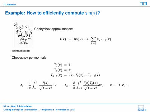
Example: How to efficiently compute sin(x)?
animaatjes.de
Chebyshev approximation:
f (x) := sin(πx) ≈n∑
k=0
ak · Tk (x)
Chebyshev polynomials:
T0(x) = 1
T1(x) = x
Tk+1(x) = 2x · Tk (x)− Tk−1(x)
a0 =1π
∫ 1
−1
f (x)√1− x2
dx , ak =2π
∫ 1
−1
f (x)Tk (x)√1− x2
dx , k = 1, 2, . . .
Miriam Mehl: 3. Interpolation
Closing the Gaps of Discretization . . . – Polynomials , November 23, 2012 3
TU Munchen
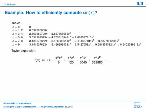
Example: How to efficiently compute sin(x)?
Table:n = 0 : 0n = 1, 2 : 0.592306858xn = 3, 4 : 2.569980700x − 2.667666686x3
n = 5, 6 : 3.091392515x − 4.753313948x3 + 1.668517810x5
n = 7, 8 : 3.139276852x − 5.136388641x3 + 2.434667195x5 − 0.4377996486x7
n = 9 : 3.141527662x − 5.166399408x3 + 2.5427059x5 − 0.5818513224x7 + 0.6402296612x9
Taylor expansion:
f (x) ≈ πx −π3x3
6+π5x5
120−π7x7
5040+
π9x9
362880− . . .
Miriam Mehl: 3. Interpolation
Closing the Gaps of Discretization . . . – Polynomials , November 23, 2012 4

TU Munchen
Example: How to efficiently compute sin(x)?
Chebyshev Polynomials – Convergence
Miriam Mehl: 3. Interpolation
Closing the Gaps of Discretization . . . – Polynomials , November 23, 2012 5

TU Munchen
Example: How to efficiently compute sin(x)?
Taylor Polynomials – Convergence
Miriam Mehl: 3. Interpolation
Closing the Gaps of Discretization . . . – Polynomials , November 23, 2012 6
TU Munchen
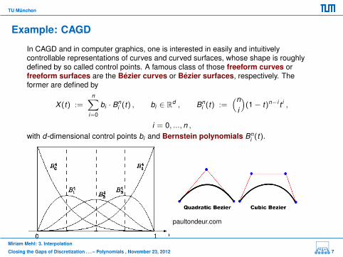
Example: CAGD
In CAGD and in computer graphics, one is interested in easily and intuitivelycontrollable representations of curves and curved surfaces, whose shape is roughlydefined by so called control points. A famous class of those freeform curves orfreeform surfaces are the Bezier curves or Bezier surfaces, respectively. Theformer are defined by
X(t) :=n∑
i=0
bi · Bni (t) , bi ∈ Rd , Bn
i (t) :=(n
i
)(1− t)n−i t i ,
i = 0, ..., n ,with d-dimensional control points bi and Bernstein polynomials Bn
i (t).
paultondeur.com
Miriam Mehl: 3. Interpolation
Closing the Gaps of Discretization . . . – Polynomials , November 23, 2012 7
TU Munchen
The Interpolation Problem
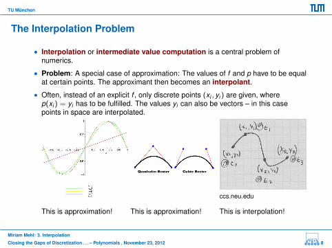
• Interpolation or intermediate value computation is a central problem ofnumerics.
• Problem: A special case of approximation: The values of f and p have to be equalat certain points. The approximant then becomes an interpolant.
• Often, instead of an explicit f , only discrete points (xi , yi ) are given, wherep(xi ) = yi has to be fulfilled. The values yi can also be vectors – in this casepoints in space are interpolated.
ccs.neu.edu
This is approximation! This is approximation! This is interpolation!
Miriam Mehl: 3. Interpolation
Closing the Gaps of Discretization . . . – Polynomials , November 23, 2012 8
TU Munchen
The Interpolation Problem
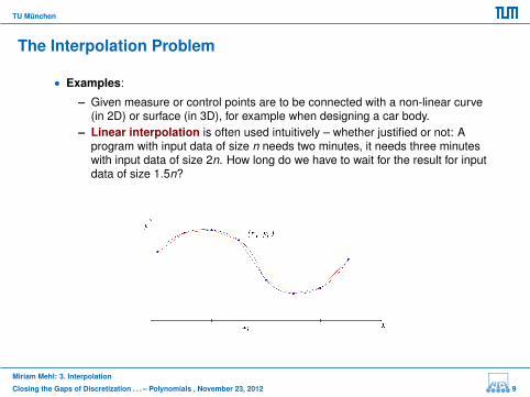
• Examples:
– Given measure or control points are to be connected with a non-linear curve(in 2D) or surface (in 3D), for example when designing a car body.
– Linear interpolation is often used intuitively – whether justified or not: Aprogram with input data of size n needs two minutes, it needs three minuteswith input data of size 2n. How long do we have to wait for the result for inputdata of size 1.5n?
Miriam Mehl: 3. Interpolation
Closing the Gaps of Discretization . . . – Polynomials , November 23, 2012 9
TU Munchen
Notation for the Problem of Interpolation
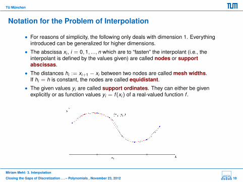
• For reasons of simplicity, the following only deals with dimension 1. Everythingintroduced can be generalized for higher dimensions.
• The abscissa xi , i = 0, 1, ..., n which are to “fasten” the interpolant (i.e., theinterpolant is defined by the values given) are called nodes or supportabscissas.
• The distances hi := xi+1 − xi between two nodes are called mesh widths.If hi = h is constant, the nodes are called equidistant.
• The given values yi are called support ordinates. They can either be givenexplicitly or as function values yi = f (xi ) of a real-valued function f .
Miriam Mehl: 3. Interpolation
Closing the Gaps of Discretization . . . – Polynomials , November 23, 2012 10
TU Munchen
• The pairs (xi , yi ) are called support points.
• Because of their simple structure, polynomials are particularly popular asinterpolants:
– Pn refers to the vector space of all polynomials with real coefficients ofdegree less or equal to n in a variable x .
– It holds that dim(Pn) = n + 1. An example for a basis is provided by themonomials x i , i = 0, ..., n:
p(x) :=n∑
i=0
ai · x i .
– As it is generally known, with the differential operator Dk for the k -thderivative with respect to x it holds:
Dn+1p = 0 ∀p ∈ Pn .
• However, the polynomial interpolation is far from being the only option:
– It is possible to glue together piecewise polynomials in order to get polynomialsplines, which have several essential advantages (see section 3.3).
– It is also possible to interpolate with rational functions (especially favored inCAGD), with trigonometric functions (see section 3.4), or with exponentialfunctions.
Miriam Mehl: 3. Interpolation
Closing the Gaps of Discretization . . . – Polynomials , November 23, 2012 11
TU Munchen
Variations of the Interpolation Problem
• There are different ways to be faced with the problem of interpolation in concreteapplications. The two most common amongst them are the following:
• simple nodes:
– This is the only case examined in this chapter.– For each of the pairwise different xi , a value yi is prescribed.– This problem of interpolation is called Lagrange interpolation– Example: Determine the quadratic polynomial p with p(−1) = p(1) = 1 and
p(0) = 0; solution: p(x) = x2.
• multiple nodes:
– For each node xi , function value yi and derivative y ′i are specified.– This interpolation problem is called Hermite interpolation.– Example: Determine the quadratic polynomial q with q(0) = q′(0) = 0 and
q′′(0) = 2; solution: q(x) = x2.– Specifying values of derivatives can be used to smoothly glue together the
polynomial pieces (i.e., without sharp bends etc.).
Miriam Mehl: 3. Interpolation
Closing the Gaps of Discretization . . . – Polynomials , November 23, 2012 12

TU Munchen
3.2. Interpolation with Polynomials
The Polynomial Interpolant and its Error
• The interpolation problem in case of polynomials:
– p ∈ Pn is called polynomial interpolant for f for the nodesa = x0 < x1 < x2 < ... < xn = b, if
p(xi ) = f (xi ) =: yi ∀i ∈ {0, 1, ..., n} .
– The definition is done analogously if, instead of a function to be interpolated,only a discrete set of data y0, . . . , yn is given.
– Therefore, the number of nodes determines the degree of the interpolationpolynomial: p has degree n, if the support points (xi , yi ) do not belong to apolynomial of lower degree.
– Thus, a large number of nodes usually results in polynomials of high degrees,which – as we will see soon – are a source of numerical problems.
– The existence and uniqueness of the solution of this interpolation problem isknown from calculus. There is always exactly one polynomial p(x) of minimaldegree that interpolates the n + 1 given points.
Miriam Mehl: 3. Interpolation
Closing the Gaps of Discretization . . . – Polynomials , November 23, 2012 13
TU Munchen
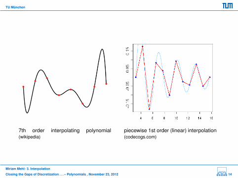
7th order interpolating polynomial(wikipedia)
piecewise 1st order (linear) interpolation(codecogs.com)
Miriam Mehl: 3. Interpolation
Closing the Gaps of Discretization . . . – Polynomials , November 23, 2012 14
TU Munchen
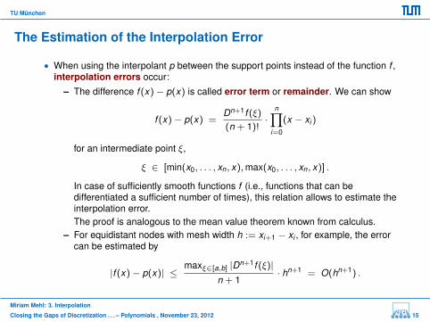
The Estimation of the Interpolation Error
• When using the interpolant p between the support points instead of the function f ,interpolation errors occur:
– The difference f (x)− p(x) is called error term or remainder. We can show
f (x)− p(x) =Dn+1f (ξ)
(n + 1)!·
n∏i=0
(x − xi )
for an intermediate point ξ,
ξ ∈ [min(x0, . . . , xn, x),max(x0, . . . , xn, x)] .
In case of sufficiently smooth functions f (i.e., functions that can bedifferentiated a sufficient number of times), this relation allows to estimate theinterpolation error.The proof is analogous to the mean value theorem known from calculus.
– For equidistant nodes with mesh width h := xi+1 − xi , for example, the errorcan be estimated by
|f (x)− p(x)| ≤maxξ∈[a,b] |Dn+1f (ξ)|
n + 1· hn+1 = O(hn+1) .
Miriam Mehl: 3. Interpolation
Closing the Gaps of Discretization . . . – Polynomials , November 23, 2012 15
TU Munchen
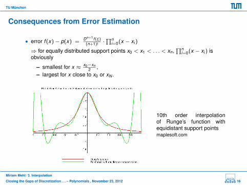
Consequences from Error Estimation
• error f (x)− p(x) = Dn+1f (ξ)(n+1)!
·∏n
i=0(x − xi )
⇒ for equally distributed support points x0 < x1 < . . . < xn,∏n
i=0(x − xi ) isobviously
– smallest for x ≈ x0−xn2 ,
– largest for x close to x0 or xN .
10th order interpolationof Runge’s function withequidistant support pointsmaplesoft.com
Miriam Mehl: 3. Interpolation
Closing the Gaps of Discretization . . . – Polynomials , November 23, 2012 16
TU Munchen
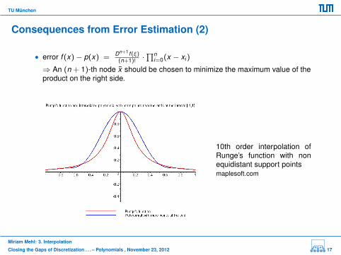
Consequences from Error Estimation (2)
• error f (x)− p(x) = Dn+1f (ξ)(n+1)!
·∏n
i=0(x − xi )
⇒ An (n + 1)-th node x should be chosen to minimize the maximum value of theproduct on the right side.
10th order interpolation ofRunge’s function with nonequidistant support pointsmaplesoft.com
Miriam Mehl: 3. Interpolation
Closing the Gaps of Discretization . . . – Polynomials , November 23, 2012 17
TU Munchen
Representation 1: Lagrange Polynomials
• The simplest approach for construction is the familiar point or incidencesampling:
– Put up p(x) with general coefficients:
p(x) :=n∑
i=0
ai · x i .
– Insert for every data point (xi , yi ) the respective value pair and solve theresulting system of n + 1 equations for the n + 1 unknowns a0, ..., an.
• An alternative approach uses Lagrange polynomials Lk (x) of degree n,
Lk (x) :=∏i:i 6=k
x − xi
xk − xi,
to determine the interpolant:
p(x) :=n∑
k=0
yk · Lk (x) .
Miriam Mehl: 3. Interpolation
Closing the Gaps of Discretization . . . – Polynomials , November 23, 2012 18
TU Munchen
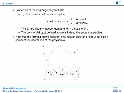
• Properties of the Lagrange polynomials:– Lk disappears at all nodes except xk :
Lk (xi ) = δik =
{1 for i = k0 otherwise.
– The Lk are linearly independent and form a basis of Pn.– The polynomial p(x) defined above is indeed the sought interpolant.
• Note that the formula above does not only deliver p(x) for a fixed x but also acompact representation of the polynomial.
Miriam Mehl: 3. Interpolation
Closing the Gaps of Discretization . . . – Polynomials , November 23, 2012 19
TU Munchen
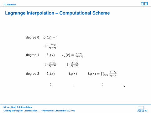
Lagrange Interpolation – Computational Scheme
degree 0 L1(x) = 1
↓ · x−x2x1−x2
degree 1 L1(x) L2(x) = x−x1x2−x1
↓ · x−x3x1−x3
↓ · x−x3x2−x3
degree 2 L1(x) L2(x) L3(x) =∏
j 6=3x−xjx3−xj
......
.... . .
Miriam Mehl: 3. Interpolation
Closing the Gaps of Discretization . . . – Polynomials , November 23, 2012 20

TU Munchen
Lagrange Interpolation – Pseudocode
for i=0 to nL[i] := 1;for j=0 to nif i neq jL[i] := L[i]*((x-x[j])/(x[i]-x[j]));
od;od;p := p + y[i]*L[i];
od;
Miriam Mehl: 3. Interpolation
Closing the Gaps of Discretization . . . – Polynomials , November 23, 2012 21
TU Munchen
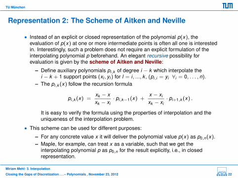
Representation 2: The Scheme of Aitken and Neville
• Instead of an explicit or closed representation of the polynomial p(x), theevaluation of p(x) at one or more intermediate points is often all one is interestedin. Interestingly, such a problem does not require an explicit formulation of theinterpolating polynomial p beforehand. An elegant recursive possibility forevaluation is given by the scheme of Aitken and Neville:
– Define auxiliary polynomials pi,k of degree i − k which interpolate thei − k + 1 support points (xl , yl ) for l = i, ..., k , (pi,i = yi ∀i = 0, . . . , n).
– The pi,k (x) follow the recursion formula
pi,k (x) =xk − xxk − xi
· pi,k−1(x) +x − xi
xk − xi· pi+1,k (x) .
It is easy to verify the formula using the properties of interpolation and theuniqueness of the interpolation problem.
• This scheme can be used for different purposes:
– For any concrete value x it will deliver the polynomial value p(x) as p0,n(x).– Maple, for example, can treat x as a variable, such that we get the
interpolating polynomial p as p0,n for the result explicitly, i.e., in closedrepresentation.
Miriam Mehl: 3. Interpolation
Closing the Gaps of Discretization . . . – Polynomials , November 23, 2012 22
TU Munchen
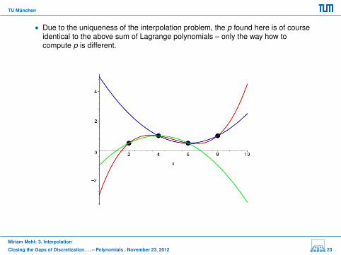
• Due to the uniqueness of the interpolation problem, the p found here is of courseidentical to the above sum of Lagrange polynomials – only the way how tocompute p is different.
Miriam Mehl: 3. Interpolation
Closing the Gaps of Discretization . . . – Polynomials , November 23, 2012 23
TU Munchen
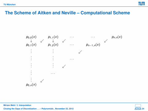
The Scheme of Aitken and Neville – Computational Scheme
p0,0(x) p1,1(x) · · · · · · pn,n(x)↓ ↙ ↓ ↙ ↙
p0,1(x) p1,2(x) · · · pn−1,n(x)...
... ↙...
... · · ·...
... ↙... · · ·... ↙
p0,n(x)
Miriam Mehl: 3. Interpolation
Closing the Gaps of Discretization . . . – Polynomials , November 23, 2012 24

TU Munchen
The Scheme of Aitken and Neville – Pseudocode
for i=0 to n dop[i,i] := y[i];
od;for k=1 to n do
for i=0 to n-k dop[i,k] := (x[k]-x)/(x[k]-x[i])*p[i,k-1] +
(x-x[i])/((x[k]-x[i])*p[i+1,k];od;
od;
Miriam Mehl: 3. Interpolation
Closing the Gaps of Discretization . . . – Polynomials , November 23, 2012 25
TU Munchen
The Scheme of Aitken and Neville
• It basically depends on the concrete problem whether the specification of a closedrepresentation for p pays off:
– If polynomial values are only to be specified for one or a few nodes, the directcomputation of the values p(x) is the better choice.
– If many evaluations are needed, the explicit computation of the polynomial(i.e., of all its coefficients) can pay off.
Miriam Mehl: 3. Interpolation
Closing the Gaps of Discretization . . . – Polynomials , November 23, 2012 26
TU Munchen
Representation 3: Newton’s Interpolation Formula
• Another possibility of representing the polynomial interpolant requires theso-called divided differences.
• With this approach, we replace the recursion for the interpolation polynomials by arecursion for the polynomial coefficients:
– From Aitken-Neville, we know
pi,k (x) =xk − xxk − xi
pi,k−1(x) +x − xi
xk − xipi+1,k
=xk
xk − xipi,k−1(x)−
xi
xk − xipi+1,k︸ ︷︷ ︸
∈Pi−k−1
+pi+1,k (x)− pi,k−1(x)
xk − xix .
– If we denote coefficient of xk−i of the polynomial pi,k by
[xi , ..., xk ]f
(called divided difference of f of order k for xi , ..., xk ), we get a recursionformula for these divided differences:
[xi , . . . , xk ]f =[xi+1, . . . , xk ]f − [xi , . . . , xk−1]f
xk − xi.
Miriam Mehl: 3. Interpolation
Closing the Gaps of Discretization . . . – Polynomials , November 23, 2012 27
TU Munchen
Newton’s Interpolation Formula (2)
• To express the polynomial p(x) using the divided differences[x0]f , . . . , [x0, . . . , xn]f , we reconsider Aitken-Neville:
p0,n(x) =xn
xn − x0p0,n−1(x) +
x0
xn − x0p1,n(x) +
p1,n(x)− p0,n−1(x)
xn − x0x
= p0,n−1 +p1,n(x)− p0,n−1(x)
xn − x0︸ ︷︷ ︸= 0 for all x ∈ {x1, . . . , xn−1}coefficient of xn−1 : [x0, . . . , xn]f
(x−x0)
= p0,n−1 + [x0, . . . , xn]fn−1∏i=0
(x − xi ).
• Thus, we get a closed representation for p(x), Newton’s interpolation formula:
p(x) := [x0]f +
[x0, x1]f · (x − x0) +
. . .
[x0, . . . , xn]f ·n−1∏i=0
(x − xi )
Miriam Mehl: 3. Interpolation
Closing the Gaps of Discretization . . . – Polynomials , November 23, 2012 28
TU Munchen
Newton’s Interpolation Formula (3)
• The appeal of this representation is its incremental character:
– When adding another node xn+1, only another summand
[x0, . . . , xn+1]f ·n∏
i=0
(x − xi )
has to be added to the actual interpolant for x0, ..., xn in its Newton form.– The computations so far do not get lost when subsequently increasing the
degree of the polynomial.– This is true neither for the Lagrange nor the Aitken-Neville representation.– The recursion formula for the divided differences also leads to a Neville-like
triangular tableau.– Neither for the scheme of Aitken and Neville nor for the divided differences
the order of nodes is relevant.
Miriam Mehl: 3. Interpolation
Closing the Gaps of Discretization . . . – Polynomials , November 23, 2012 29
TU Munchen
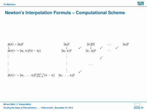
Newton’s Interpolation Formula – Computational Scheme
p(x) = [x0]f [x0]f [x1][f ] · · · [xn]f↓ ↓ ↙ ↓ ↙ ↙p(x)+ = [x0, x1]f (x − x0) [x0, x1]f [x1, x2]f · · ·...
... ↙...
... · · ·...
... ↙p(x)+ = [x0, . . . , xn]f
∏n−1i=0 (x − xi ) [x0, . . . , xn]f
Miriam Mehl: 3. Interpolation
Closing the Gaps of Discretization . . . – Polynomials , November 23, 2012 30
TU Munchen
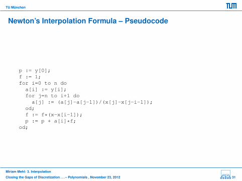
Newton’s Interpolation Formula – Pseudocode
p := y[0];f := 1;for i=0 to n do
a[i] := y[i];for j=n to i+1 doa[j] := (a[j]-a[j-1])/(x[j]-x[j-i-1]);
od;f := f*(x-x[i-1]);p := p + a[i]*f;
od;
Miriam Mehl: 3. Interpolation
Closing the Gaps of Discretization . . . – Polynomials , November 23, 2012 31
TU Munchen
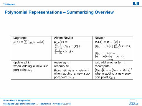
Polynomial Representations – Summarizing Overview
Lagrange Aitken-Neville Newtonp(x) =
∑ni=0 yi · Li (x) p0,n(x) =
xn−xxn−x0
· p0,n−1(x)+x−x0xn−x0
· p1,n(x)
pn(x) = pn−1(x)+
[x0, . . . , xn]f∏n−1
i=0 (x−xi ),
[x0, . . . , xn]f =[x1,...,xn ]f−[x0,...,xn−1]f
xn−x0update all Liwhen adding a new sup-port point xn+1
reuse p0,n,recomputep1,n+1, p2,n+1, . . . , pn,n+1when adding a new sup-port point xn+1
just add another term,recompute[xn+1]f , . . . , [x0, . . . , xn+1]fwhenn adding a new sup-port point xn+1.
Miriam Mehl: 3. Interpolation
Closing the Gaps of Discretization . . . – Polynomials , November 23, 2012 32
TU Munchen
The Condition of Polynomial Interpolation
• How well-conditioned or ill-conditioned is the problem of interpolation?
– Input data: the nodes xi , the sampling values yi , as well as the intermediatepoint x at which the function value is to be reconstructed by interpolation.
– Solution: the value y := p(x)
• Therefore, there are different ’condition numbers’ – depending on the input datawith respect to which the sensitivity is to be examined.
• It is easiest to describe the sensitivity of p(x) regarding variations in the point ofevaluation x – it is just described by p′(x) and, hence, it is bounded on [a, b] in thecase of polynomials, but it can become very big, particularly with high degrees ofp(x).
Miriam Mehl: 3. Interpolation
Closing the Gaps of Discretization . . . – Polynomials , November 23, 2012 33
TU Munchen
The Condition of Polynomial Interpolation (2)
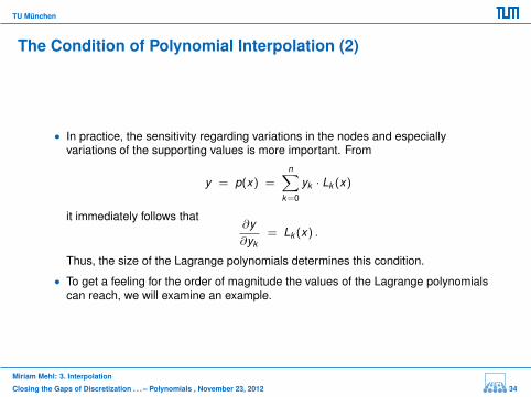
• In practice, the sensitivity regarding variations in the nodes and especiallyvariations of the supporting values is more important. From
y = p(x) =n∑
k=0
yk · Lk (x)
it immediately follows that∂y∂yk
= Lk (x) .
Thus, the size of the Lagrange polynomials determines this condition.
• To get a feeling for the order of magnitude the values of the Lagrange polynomialscan reach, we will examine an example.
Miriam Mehl: 3. Interpolation
Closing the Gaps of Discretization . . . – Polynomials , November 23, 2012 34
TU Munchen
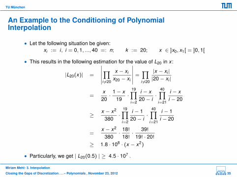
An Example to the Conditioning of PolynomialInterpolation
• Let the following situation be given:xi := i, i = 0, 1, ..., 40 =: n; k := 20; x ∈ ]x0, x1[ = ]0, 1[
• This results in the following estimation for the value of L20 in x :
|L20(x)| =
∣∣∣∣∣∣∏i 6=20
x − xi
x20 − xi
∣∣∣∣∣∣ =∏i 6=20
|x − xi ||20− xi |
=x20·
1− x19
·19∏
i=2
i − x20− i
·40∏
i=21
i − xi − 20
≥x − x2
380·
19∏i=2
i − 120− i
·40∏
i=21
i − 1i − 20
=x − x2
380·
18!
18!·
39!
19! · 20!
≥ 1.8 · 108 · (x − x2)
• Particularly, we get | L20(0.5) | ≥ 4.5 · 107 .
Miriam Mehl: 3. Interpolation
Closing the Gaps of Discretization . . . – Polynomials , November 23, 2012 35

TU Munchen
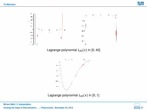
• This is an fundamental result: Small errors in central supporting values aredramatically increased at the borders of the examined interval by polynomialinterpolation.
• For large n (7 or 8 and up), polynomial interpolation is extremely ill-conditionedand therefore basically useless.
• For this reason, better methods must be found in this regard.
Miriam Mehl: 3. Interpolation
Closing the Gaps of Discretization . . . – Polynomials , November 23, 2012 36
TU Munchen
Lagrange polynomial L20(x) in [0, 40]
Lagrange polynomial L20(x) in [0, 1]
Miriam Mehl: 3. Interpolation
Closing the Gaps of Discretization . . . – Polynomials , November 23, 2012 37