international trade policy
TRANSCRIPT

1
LECTURE NOTES
in
INTERNATIONAL TRADE POLICY (*)
(ITR402)
Cevat Gerni
Beykent University/İstanbul
2010
(*) These lecture notes mostly depend on the textbooks of Dominick Salvatore (International Economics, 9e), Paul R.Krugman & Maurice Obstfeld (International Economics, 3e), Gregory Mankiw (Principals of Economics, 4e) and Halil Seyidoğlu (Uluslararası İktisat, 17e), with our own contributions.

2
1. Introduction
In the international Economics course, we examined the theoretical basis of trade among
nations:
- Why do nations trade?
- What are the gains of nations from trade?
- At what prices do they trade (terms of trade)?
- And, some related subjects (transportation costs, environmental standards,
economic growth/development – trade interactions, and so on)
In this course of International Trade Policy, we will analyze the trade policies.
Before analyzing the effects of trade policies, we should learn the tools of welfare economics,
because we will use them to understand the effects of trade policies.
In this context, we will learn
Consumer surplus
Producer surplus
Market efficiency
The deadweight loss
After this introductory information, some of the subjects of trade policies are following:
How free trade affect welfare in an “exporting country”?
How free trade affect welfare in an “importing country”?
The effects of a “tariff” (who gains and who loses from a tariff imposition?)
The effects of a “quota” (who gains and who loses from a quota limitation?)
The arguments for restricting trade (for protectionism)
The rate of effective protection
Theory of economic integration
3
2. Tools of welfare economics
What is the best price that maximizes the total welfare of consumers and
producers?
To answer this question, we should know the concepts of consumer surplus and
producer surplus.
Yet, before analyzing the consumer and producer surplus, let’s give the answer
to the question above:
‘The equilibrium of supply and demand in a market maximizes the total
benefits received by buyers and sellers.’
In other words, ‘the price that balances the supply and demand for a
commodity is the best one because it maximizes the total welfare of the
consumers and producers.’
2a. Consumer Surplus
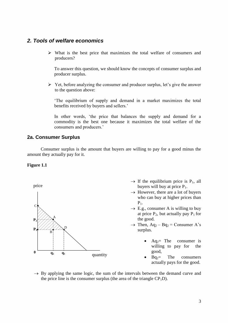
Consumer surplus is the amount that buyers are willing to pay for a good minus the
amount they actually pay for it.
Figure 1.1
If the equilibrium price is P1, all
buyers will buy at price P1.
However, there are a lot of buyers
who can buy at higher prices than
P1.
E.g., consumer A is willing to buy
at price P2, but actually pay P1 for
the good.
Then, Aq2 – Bq2 = Consumer A’s
surplus.
Aq2= The consumer is
willing to pay for the
good,
Bq2= The consumers
actually pays for the good.
By applying the same logic, the sum of the intervals between the demand curve and
the price line is the consumer surplus (the area of the triangle CP1D).
0 q2 q1
A
D
C
B P1
P2
price
quantity

4
Figure 1.2
At price P1, the consumer surplus
is AP1C.
At price P2, the consumer surplus
is AP2D.
A lower price raises
consumer surplus. On the
contrary, a higher price falls
consumer surplus.
2b. Producer Surplus
Figure 1.3
We apply the same logic.
All producers (sellers) sell at price
P1. (Equilibrium price)
But there are many producers who
can sell at lower prices.
E.g. producer A, whose cost is Aq2
(=P2) is able to sell at price P2 but
she actually sells at price P1)
Then, P1-P2 (Bq2- Aq2) is the
producer A’s surplus.
All producers up to point C on the
supply curve benefit from the
difference between the actual price
and the price they are willing to
sell.
Then, P1CD is the producer surplus,
the area above the supply curve and
below the price line.
q
P
A
P2 D
C
q1 q2
P1
0
P
q
A
B C
q1 q2
S
D
0
P1
P2

5
Figure 1.4
A higher price raises the producer
surplus.
Because when price rises, the less
efficient firms can meet their high costs and
start to produce. Plus, initial firms produce
more to earn more.
At price P1, the producer surplus is
the area of the triangle P1AC. (Initial
producer surplus)
When price rises (from P1 to P2), the
producer surplus increases by the
area of P1ABP2.
* P1ADP2 is the increase in
initial producers’ surplus.
(Additional producer surplus
to initial producers)
* ABD is the producer surplus
to new producers.
2c. Total Surplus
Figure 1.5
Total Surplus - the sum of consumer
and producer surplus - is the area
between the supply and demand
curves up to the equilibrium quantity.
Additional
producer surplus to
initial producers’
Producer
surplus to new producers
Initial producer
surplus
A
B
C
D
q1 q2
S
P2
P1
D
S
E
q Equilibrium
quantity
q
P
P
Equilibrium
price
Consumer
surplus
Producer
surplus

6
Figure 1.6
Recall that the demand curve
reflects ‘the value to buyers’
and that the supply curve
reflects ‘the cost to sellers’.
At quantities less than the
equilibrium quantity, the value
to buyers exceeds the cost to
sellers.
At quantities greater than the
equilibrium quantity, the cost to
sellers exceeds the value to
buyers.
Therefore, the market
equilibrium maximizes the sum
of producer and consumer
surplus.
As a result, any policy imposing
a price less or greater than
equilibrium price causes a
decrease in total surplus.
2d. Market Efficiency and Market Failure
Keep in mind that these analyses depend on the assumptions of freely
competitive markets.
When the assumptions of perfectly competitive market do not hold, our
conclusion that the market equilibrium is efficient may no longer be true.
‘Market power’ and ‘externalities’ can distort the market efficiency.
This phenomenon is called ‘market failure’.
When markets fail, public policy can potentially remedy the problem and
increase economic efficiency.
Despite the possibility of market failure, the invisible hand of the marketplace
is extraordinarily important.
In many markets the assumptions of free markets work well, and the
conclusion of market efficiency applies directly.
The analysis of market efficiency can be used to shed light on the effects of
various government policies.
Two policies will be considered; taxation policy and international trade policy.
0
Value
to
buyers
cost to
sellers
cost to
sellers
Value
to
buyers
qe
equilibrium
quantity
E
S
D
q
P
Value to
buyers is
greater than
cost to sellers
Value to
buyers is less
than cost to
sellers

7
3. The Deadweight Loss of Taxation
Figure 1.7 (The effect of a Tax)
Note: For simplicity, the shift of the
supply curve to the left with the effect of
tax will not be shown in other graphs.
Figure 1.8 (Tax Revenue)
Now, what happened with the tax?
With the tax,
The quantity sold in the
market decreased (from q1
to q2)
The price that buyers pay
differentiated from the
price that sellers receive.
The total surplus decreased
by the area of triangle
ABE.
This area (ABE) is called
deadweight loss. Because
the market contracted by
the amount of q1q2; some
sellers and buyers left the
market.
Price
sellers
receive
Price
without
tax
Price
buyers
pay
size of
tax
E1
E2
P1
P3
P2
q2 q1
quantity
without tax
quantity
with tax
S’
S
D
q
P
A
PS
E
PB
S
B
Tax
revenue
( Txq2 )
x
0
D
Size of the tax
( quantity
sold )
( the size of
the tax) = Tax revenue that the
government collects
q2 q1

8
Figure 1.9 (Welfare effects of a tax)
WITHOUT
TAX
WITH TAX CHANGE
Consumer Surplus A+B+C A -(B+C)
Producer Surplus D+E+F F -(D+E)
Tax Revenue None B+D +(B+D)
Total Surplus A+B+C+D+E+F A+B+D+F
-(C+E)*
* : The area C+E shows the fall in total surplus and is the deadweight loss of the tax.
Definition of Deadweight Loss :
It is the fall in total surplus that results from a market distortion, such as a tax.
4. The Determinants of Deadweight Loss
What determines whether the deadweight loss from a tax is large or small?
The answer is the price elasticities of supply & demand.
Figure 1.10
size of
tax
(b)
q
D
deadweight
loss is large
elastic
supply
P
Ps
P1
PB
PB
S
D
F
E D
C B
A
q2 q1
P
D
q
(a)
inelastic
supply
deadweight
loss is small
size of
the tax

9
The Result: the greater (smaller) the elasticities of supply and demand,
the greater (smaller) the deadweight loss of a tax.
5. The Deadweight Loss and Tax Revenue As Taxes Vary
What happens to the deadweight loss and tax revenue when the size of a tax changes?
Figure 1.11
In these three panels, the
demand and supply curves are
held constant.
Only the ‘size of tax’
changes, in order to show
how tax revenue changes
when the size of tax
changes.
PS
B
PB
B
P
q2 q1
deadweight
loss
tax
revenue
S
D
deadweight
loss is large
S
size
of
tax
q
P elastic
demand S
size
of
tax
q
P
deadweight
loss is small
(c)
inelastic
demand
PS
B
PB
B
q2 q1
S
D
q
P
deadweight
loss
tax
revenue
P
(a) small tax
q2 q1
D
S P
deadweight
loss
q
tax
rev
en
ue
(d)
q
(b) medium tax
(c) large tax

10
Note that, for the small tax in panel (a), the area of deadweight loss triangle is quite
small.
But as the size of the tax rises in panel (b) and (c), the deadweight loss grows
larger and larger. (ah / 2 → 2a.2h / 2 = 2ah = 4 x (ah / 2) (Area of a triangle is half the
base times the height. If you increase the base twice, the area, the deadweight loss,
increases four times.)
Indeed the deadweight loss of a tax rises even more rapidly than the size of the tax.
From this analysis, we can conclude that as the tax size rises, first the tax revenue gets
larger and then it gets smaller because the market shrinks.
This case can be illustrated by the ‘Laffer Curve’. (Because Arthur Laffer first
pointed out this fact in 1974).
Figure 1.12
As it is shown in Figure 1.12, the tax revenue rises to a certain size of the tax
and after that it starts to fall.
The Reagan Administration adopted this policy in 1980s. (R. Reagan,
republican, 1980-89)
But subsequent history failed to confirm Laffer’s conjecture that lower tax
rates would raise tax revenue.
When Reagan cut taxes after he was elected, the result was less tax revenue,
not more.
The views of Laffer and Reagan became known as ‘supply-side economics’
The validity of supply-side economics is debated. However, there is no debate
about the general lesson:
‘How much revenue the government gains or loses from a tax change cannot
be computed just by looking at tax rates. It also depends on how the tax change
affects people’s behavior.’ (Elasticities are important.)
To
Tax size
Tax
Revenue

11
CHAPTER 2
AN APPLICATION FOR WELFARE ECONOMICS
(International Trade)
In this chapter we will see:
How international trade affects economic well-being,
Who gains and who loses from free trade among countries, and
How do the gains compare to the losses?
To answer these questions we’ll use the tools of supply, demand, consumer and
producer surplus and so on.
In the following analyses, we suppose the country is Turkey, and the good is steel.
2.1. The Equilibrium without International Trade
Figure 2.1
When Turkey cannot
trade in world
markets, the price
adjusts to balance
domestic supply and
demand.
This figure shows
consumer and
producer surplus in
equilibrium without
international trade for
the steel market.
Producer
surplus
E
Consumer surplus
Price
of
steel
q*
P*
P*=equilibrium price
q*=equilibrium quantity
Domestic
Supply
Domestic
Demand
quantity of steel

12
2.2 The Winners and Losers from Trade
Figure 2.2 (In the case of exporting country)
We suppose that Turkey is an
exporting country. And
assume that it is a small
country, which means that its
actions do not affect world
price. It is a price taker.
Once trade is allowed, the
domestic price rises to equal
the world price.
2.3. How Free Trade Affects Welfare in an ‘Exporting Country’?
We should compare the changes in producer and consumer surplus before and after trade.
Figure 2.3
Before Trade After Trade Change
Consumer Surplus A+B A -B
Producer Surplus C B+C+D +(B+D)
Total Surplus A+B+C A+B+C+D +D* *: The area D shows the increase in total surplus and represents the gains from trade.
E
D
Price
before
trade
exports
Price
after
trade
Domestic
quantity
supplied
Domestic
quantity
demanded
Domestic
Demand
world price
Domestic
Supply
C
B
A exports
Price
before
trade
Price
after
trade
Price of
steel
Domestic
Demand
World price
Domestic
Supply
quantity of steel

13
This analysis of an exporting country yields two conclusions:
1) When a country allows trade and becomes an exporter of a good, domestic producers
of the good are better off, and domestic consumers of the good are worse off.
2) Trade raises the economic well-being of a nation in the sense that the gains of the
winners (B+D) exceed the losses of the losers. (-B)
2.4. How free trade affects welfare in an ‘importing country’?
Again, we should compare the changes in producer and consumer surplus before and
after trade.
Figure 2.4.
Turkey is a small country.
It is a price taker.
Once trade is allowed, the
domestic price falls to
equal the world price.
Before Trade After Trade Change
Consumer Surplus A A+B+D +(B+D)
Producer Surplus B+C C -B
Total Surplus A+B+C A+B+C+D +D*
*: The area D shows the increase in total surplus and represents the gains from trade.
This analysis of an importing country yields two conclusions parallel to those for an
exporting country:
1) When a country allows trade and becomes an importer of a good, domestic
consumers of the good are better off, and domestic producers of the good are
worse off.
2) Trade raises the economic well-being of a nation in the sense that the gains of
the winners (B+D) exceed the losses of the losers (-B)
Now that we have completed our analysis of trade, we can conclude that ‘trade can
make everyone better off’
world price
C
domestic
quantity
demanded
domestic
quantity
supplied
imports
D B
A
Price
after
trade
Price
before trade
Price
of
steel
quantity of
steel
domestic
demand
domestic
supply
14
If Turkey opens up its steel market to international trade the change will create
winners and losers, regardless of whether Turkey ends up exporting or importing steel.
In either case, however, the gains of the winners exceed the losses of the losers, so
the winners could compensate the losers and still be better off.
In this case, trade can make everyone better off. But will trade make everyone
better off? Probably NOT.
In practice, compensation for the losers from international trade is rare.
Without such compensation, opening up to international trade is a policy that
expands the size of the economic pie, while perhaps leaving some participants in the
economy with a small slice.
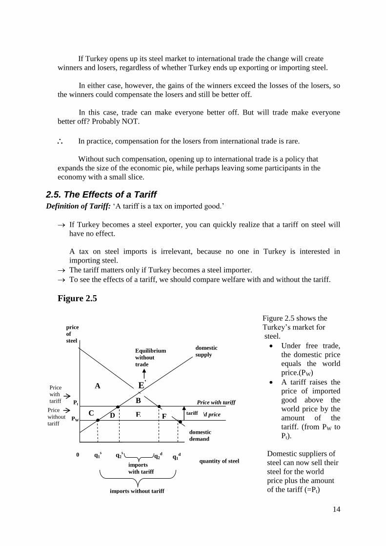
2.5. The Effects of a Tariff
Definition of Tariff: ‘A tariff is a tax on imported good.’
If Turkey becomes a steel exporter, you can quickly realize that a tariff on steel will
have no effect.
A tax on steel imports is irrelevant, because no one in Turkey is interested in
importing steel.
The tariff matters only if Turkey becomes a steel importer.
To see the effects of a tariff, we should compare welfare with and without the tariff.
Figure 2.5
Figure 2.5 shows the
Turkey’s market for
steel.
Under free trade,
the domestic price
equals the world
price.(PW)
A tariff raises the
price of imported
good above the
world price by the
amount of the
tariff. (from PW to
Pt).
Domestic suppliers of
steel can now sell their
steel for the world
price plus the amount
of the tariff (=Pt)
Pt
Orld price D
PW
Price
with
tariff
Price
without
tariff
0
Equilibrium
without
trade
imports without tariff
imports
with tariff
q1d q2
d q2s
q1s
E’
price
of
steel
F E
B
C
A
tariff
Price with tariff
domestic
demand
domestic
supply
quantity of steel

15
Thus the price of steel -both imported and domestic- rises by the amount of tariff
and is, therefore, closer to the price that would prevail without trade.
The change in price affects the behavior of domestic buyers and sellers
Prices and quantities:
Without tariff:
PW is the world price.
q1s
is the quantity supplied by domestic sellers.
q1d is the quantity demanded by domestic buyers.
q1s- q1
d is the amount which is imported (under free trade/with no restriction).
With tariff:
Pt is the price with tariff
q2s is the quantity supplied by the domestic seller after the tariff.(Because
price rose/because of the law of supply)
q2d is the quantity demanded by the domestic buyers after the tariff.
(Because of the law of demand)
q2s-q2
d is the amount which is imported after the tariff.
Thus, ‘the tariff reduces the quantity of imports and moves the domestic
market closer to its equilibrium without trade’.
Now consider the gains and losses from the tariff:
Because the tariff raises the domestic price, domestic sellers are better
off, and domestic buyers are worse off.
The government raises revenue.
To measure these gains and losses, we look at the changes in consumer surplus,
producer surplus and government revenue.
Before Tariff After Tariff Change
Consumer Surplus A+B+C+D+E+F A+B -(C+D+E+F)
Producer Surplus G C+G +C
Government Revenue None E +E
Total Surplus A+B+C+D+E+F+G A+B+C+E+G -(D+F)* *: The area D+F shows the fall in total surplus and represents the deadweight loss of the tariff.
Area D represents the deadweight loss from the ‘overproduction’ of
steel. (Because some resources are used at higher costs)
Area F represents the deadweight loss from the
‘underconsumption’.(Because the society reduces its consumption)
2.6 The Effects of an Import Quota
Definition of Import Quota: ‘An import quota is a limit on the quantity of imports’.
Imagine that the Turkish government distributes a limited number of import licenses.
Each license gives the license holder the right to import 1 ton of steel into Turkey
from abroad.
16
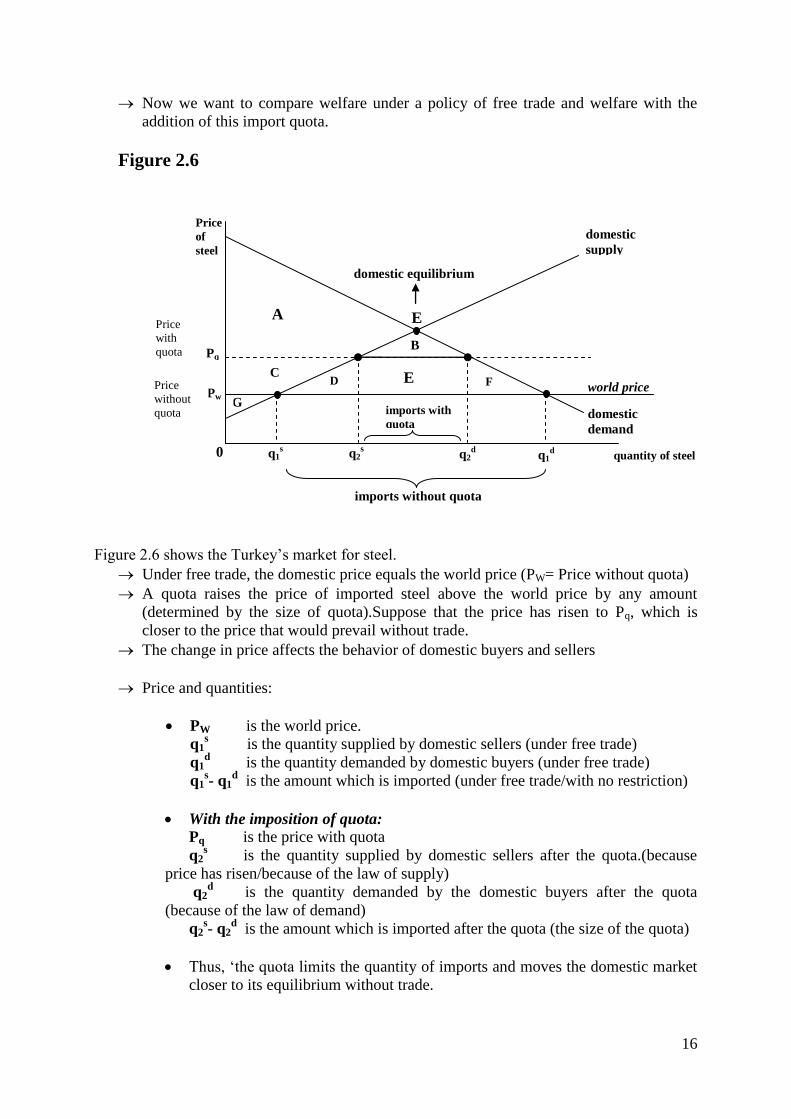
Now we want to compare welfare under a policy of free trade and welfare with the
addition of this import quota.
Figure 2.6
Figure 2.6 shows the Turkey’s market for steel.
Under free trade, the domestic price equals the world price (PW= Price without quota)
A quota raises the price of imported steel above the world price by any amount
(determined by the size of quota).Suppose that the price has risen to Pq, which is
closer to the price that would prevail without trade.
The change in price affects the behavior of domestic buyers and sellers
Price and quantities:
PW is the world price.
q1s is the quantity supplied by domestic sellers (under free trade)
q1d is the quantity demanded by domestic buyers (under free trade)
q1s- q1
d is the amount which is imported (under free trade/with no restriction)
With the imposition of quota:
Pq is the price with quota
q2s is the quantity supplied by domestic sellers after the quota.(because
price has risen/because of the law of supply)
q2d is the quantity demanded by the domestic buyers after the quota
(because of the law of demand)
q2s- q2
d is the amount which is imported after the quota (the size of the quota)
Thus, ‘the quota limits the quantity of imports and moves the domestic market
closer to its equilibrium without trade.
0
domestic equilibrium
imports without quota
imports with
quota
F
q1d q2
d q2s
q1s
D E
B
G
C
A E
Pw
Price
with
quota Pq
quantity of steel
Price
of
steel
world price
domestic
demand
domestic
supply
Price
without
quota

17
Now consider the gains and losses from the quota:
Note that the effects are identical with those of a tariff.
Because the quota raises the domestic price, domestic sellers are better
off, and domestic buyers are worse off.
However, the surplus from the quota is different from the case of a tariff.
(This is important and the distinctive character of a quota from a tariff).
To measure the gains and losses, we look at the changes in consumer surplus, producer
surplus, and quota surplus.
(Because a quota is distributed to the license holders, the surplus from the quota can be
called ‘License-holder surplus’).
Before Quota After Quota Change
Consumer Surplus A+B+C+D+E+F A+B -(C+D+E+F)
Producer Surplus G C+G +C
Lisence-Holder Surplus None E +E
Total Surplus A+B+C+D+E+F+G A+B+C+E+G -(D+F)*
*: The area D+F shows the fall in total surplus and represents the deadweight loss of the quota.
Again, if you compare the analysis of import quotas in Figure 2.6 with the analysis of
tariffs in Figure 2.5, you will see that they are essentially identical.
Both tariffs and import quotas,
raise the domestic price of the good,
reduce the welfare of domestic consumers,
increase the welfare of domestic producers, and
cause deadweight losses.
There is only one difference between these two types of trade restriction:
A tariff raises revenue for the government, whereas
An import quota creates surplus for license holders.
But tariffs and import quotas can be made to look even more similar by using
some mechanism to allocate the import licenses.
One mechanism is that the government can set the license fee as high as
the price differential (between the world price and the domestic price
with quota)
If the government does this, the license fee for imports works exactly
like a tariff.
On the other hand, when the government imposes a quota, the licenses
will go to those who spend the most resources lobbying the
government. In this case, there is an ‘implicit license fee’-the cost of
lobbying.
The revenues from this fee are spent on lobbying expenses. Then the deadweight
losses from this type of quota include not only the losses from overproduction

18
(area D) and underconsumption (area F) but also whatever part of the license-
holder surplus (E) is wasted on the cost of lobbying.
2.7 The Lessons for Trade Policy
By considering the analyses so far, we can arrive at some conclusions: (Suppose the
traded good is steel, the country is Turkey).
Once trade is allowed (i.e., in case of free trade), the
price of steel is driven to equal the price prevailing
around the world.
Two cases are possible:
First, if the world price is higher than the price
in Turkey;
Our price rises,
We consume less (because of the law of
demand)
Our suppliers produce more,
Turkey becomes a steel exporter, (This
occurs because Turkey has a comparative
advantage in producing steel)
Second, conversely, if the price is lower than the price
in Turkey;
Our price falls,
We consume more (because of the law of
demand)
Our suppliers produce less ( because of the
law of supply)
Turkey becomes a steel importer (This
occurs because other countries have a
comparative advantage in producing steel.)
The answer depends on whether the price rises or
falls when trade is allowed.
(In other words, it depends on whether Turkey
becomes an exporting or importing country).
1) If the price rises (i.e., Turkey exports),
-producers of steel gain,
-consumers of steel lose.
2) If the price falls (i.e., Turkey imports),
-consumers gain,
-producers lose.
1. What
happens to
domestic
price?
2. What
happens to the
quantity?
3. Who gains and
who losses from free
trade, and do the
gains exceed the
losses

19
3) In both cases, the gains are larger than the
losses. Thus, free trade raises the total welfare
of Turkish people.
A tariff, like most taxes, has deadweight losses:
The revenue raised can be smaller than the losses to
the buyers and sellers.
An import quota works much like a tariff and cause similar deadweight
losses.
Thus, the best policy, from the standpoint of efficiency, is to allow trade
without a tariff or an import quota.
Then, why do countries restrict trade? We will see the arguments! But, before that, we
need to consider other benefits of trade beyond those emphasized in the standard analysis.
2.8 Other Benefits of International Trade
Our conclusions so far have been based on the standard analysis of international
trade.
As we have seen, there are winners and losers when a nation opens itself up to trade,
but the gains to the winners exceed the losses of the losers.
Yet, the case for free trade can be made even stronger. There are several other
economic benefits of trade beyond those explained in the standard analysis.
Here are some of these other benefits (in short) (Dynamic Benefits)
Increased variety of goods: Goods produced in different countries are not exactly the same. Free trade
gives consumers in all countries greater variety from which to choose.
Lower costs through economies of scale: Some goods can be produced at low cost only if they are produced in large
quantities-a phenomenon called ‘economies of scale’.
Free trade gives firms in small countries access to larger world markets and
allows them to realize economies of scale more fully.
Increased Competition: A company shielded (defended) from foreign competitors is more likely to
have market power. This is a type of market failure.
Opening up trade fosters competition and gives the invisible hand a better
chance to work its magic.
4. Should a tariff or
an import quota be
part of the trade
policy?

20
Enhanced Flow of Ideas: Technological advances, managerial skills and like are available through
international trade.
For example, the best way for a poor nation to learn about the computer
revolution is to buy some computers from abroad, rather than trying to make them
domestically.
2.9 The Arguments for Restricting Trade
Why do governments restrict trade?
Put differently, why do the representatives of some industries want their production to
be protected from foreign producers?
Here are the main arguments for trade restrictions:
1) The Jobs Argument
2) The National Security Argument
3) The Infant Industry Argument
4) The Unfair Competition Argument
5) The Protection As a Bargaining-Chip Argument
1) The Jobs Argument
-Opponents of free trade often argue that
‘Trade with other countries destroys
domestic jobs’
(It reduces employment in the steel industry)
(some workers will be laid off.)
-Advocates of free trade claim that
Yet free trade ‘creates’ new jobs at the
same time.
Under comparative advantage, workers
will eventually find new jobs. Even though
the transition may impose hardship on some
workers in the short run, free trade allows a
high standard of living as a whole.
2) The National Security Argument
When an industry is threatened with competition from other countries,
-Opponents of free trade often argue that
The industry is ‘vital’ for national
security.
(e.g., steel is used to make guns and
weapons. If a war broke down, the nation
might be unable to produce enough steel and
weapons to defend their country).
-Economists acknowledge that
Protecting key industries may be
‘appropriate’ when there are ‘legitimate
concerns’ over national security.

21
Yet, this argument may be used too
quickly by producers eager to gain at
consumers’ expense.
(e.g., the U.S. watch making industry long
argued that it was vital for national security,
claiming that its skilled workers would be
necessary in war time.)
It is tempting for those in an industry to exaggerate their role in order to obtain
protection from foreign competition.
3) The Infant-Industry Argument
-New industries sometimes argue for
‘temporary’ trade restrictions. Because
After a period of protection, these
industries will ‘mature’ and ‘be able to
compete’ with foreign competitors.
-Similarly, older industries sometimes argue
that
They need ‘temporary protection’ to
help them adjust to new conditions.
-Economists are often ‘skeptical’ about
such claims. Because
First, this argument is difficult to
implement in practice: which industries will
eventually be profitable.
So, ‘picking winners’ is extraordinarily
difficult.
Second, it is made even more difficult
by the ‘political process’.
(Politically powerful industries can obtain
protection permanently.)
Third, theoretically, even though an
industry is young and unable to compete
against foreign rivals, it can be profitable in
the long run. Therefore, ‘protection is not
necessary for an industry to grow’ (many
industries incur temporary losses in the hope
of becoming profitable in the future, and
many firms succeed without protection; such
as internet firms).

22
4. The Unfair Competition Argument
-A common argument is that
Free trade is desirable only if all
countries play by the same rules.
If firms in different countries are subject
to different rules, then it is unfair to expect
the firms to compete in international
marketplace. Therefore, domestic industry
facing unfair competition should be
protected.
(Subsidies are an example of this case…)
-Advocates of free trade say that
Certainly, domestic producers would
suffer from subsidized prices. But ‘domestic
consumer would benefit from the low price’.
‘And the taxpayers of subsidizing
country bear the burden.’
5. The Protection as a Bargaining-Chip Argument
-This argument (for trade restrictions)
concerns
The strategy of bargaining
This argument claims that
‘Trade restrictions can be useful when
we bargain with our trading partners.’
This argument claims that
The threat of a trade restriction can help
‘remove’ a trade restriction already imposed
by a foreign government.
(A country might threaten to impose a tariff
on its imported goods unless its trading
partner removes restrictions on the goods of
that country).
An example of this occurred in
23
1999.The U.S. government accused
Europeans of restricting the import of U.S.
bananas. The United States placed 100
percent tariffs on a range of European
products.
In the end, not only were Europeans
denied the benefits of American bananas, but
also Americans were denied the benefits of
European cheese!
The problem with this bargaining strategy is
that
‘The threat may not work’
If it doesn’t work, the country has a
difficult choice:
- either it implements the trade
restriction, and accordingly reduces its own
economic welfare,
- or it can back down from its threat,
and accordingly loses prestige in
international affairs.
CONCLUSION: Economists and the general public often ‘disagree’ about the
‘free trade’. There is an eternal battle between opponents and advocates of free
trade.
2.10 The New Protectionism
So far, we examined
The traditional trade barriers (tariffs and quotas) and their welfare effects (static
effects)
Other benefits of trade (dynamic effects) and
Arguments for restricting trade.
While tariffs and quotas are traditional tools for the purpose mainly to protect
domestic industries, there are other barriers which have become more important in the
world of today.
These trade barriers are seen as ‘the tools of new protectionism’.
The tools of new protectionism are :
1) Voluntary export restraints,
2) Technical, administrative, and other regulations,
3) International cartels,
4) Dumping,
5) Export Subsidies.

24
1) Voluntary Export Restraints (VERs):
With such an arrangement, an importing country induces another nation to reduce its
exports of a commodity ‘voluntarily’.(under the threat of higher all-round
restrictions).
VERs sometimes called ‘orderly marketing arrangements’
When VERs are successful, they have all the economic effects of equivalent import
quotas, except that :
They are administered by the exporting country,
So the revenue effect is captured by foreign exporters.
Voluntary export restraints might be less effective in limiting imports than import
quotas because the exporting nations agree only reluctantly to curb their exports.
Foreign exporters also tend to fill their quota with higher-quality and higher-priced
units of their product over time. This product upgrading was clearly evident in the
case of Japanese voluntary restraint on automobile exports to the United States.(For
an example of VERs, see Case Study 9-1, p. 33 of this Lecture Notes)
There were such agreements between industrial countries (U.S., E.U. and Canada)
and developing countries (see p.291-293, Salvatore, 9e). The Uruguay Round
required the phasing out of all VERs by the end of 1999 and the prohibition on the
imposition of new VERs.
2) Technical, Administrative and Other Regulations:
These include:
Safety Regulations (for automobile and electrical equipment)
Health Regulations (for the hygienic production and packing of imported food
products)
Labeling Requirements (showing origin and contents)
Note: While many of these regulations serve legitimate purposes, some are only
veiled disguises for restricting imports.
Government Procurement policies (laws requiring governments to buy from
domestic suppliers)
25
Border Taxes (rebates for internal ‘indirect taxes’ given to exporters and
imposed - in addition to the tariff - on importers); e.g. sales and value-added
taxes.
International Commodity Agreements (for the stabilization of export prices,
they restrict the production and selling of the certain commodities; e.g.
International Tin Agreement, set up in 1956, ).
Multiple Exchange Rates (higher exchange rates on luxury and nonessential
imports and lower exchange rates on essential imports).
3) International Cartels:
An international cartel is an organization of suppliers of a commodity located
in different nations that agrees to restrict output and exports of the commodity
with the aim of increasing the total profit.
The power of international cartels cannot easily be countered because they do
not fall under the jurisdiction of any one nation.
OPEC is the example.
4) Dumping:
Dumping is the export of a commodity at below cost or at least the sale of a
commodity at a lower price abroad then domestically.
Dumping is classified into three types:
o Persistent Dumping: (International Price Discrimination;
continuous tendency)
o Predatory Dumping: (Yıkıcı Damping)
It is the temporary sale of a commodity at below cost or at a lower
price abroad to drive foreign producers out of business.
o Sporadic Dumping:
It is the ‘occasional sale of a commodity at below cost (or at a lower
price abroad then domestically) in order to unload an unforeseen and
temporary surplus of the commodity without having to reduce
domestic prices.
Trade restrictions are applied to protect domestic industries from unfair
competition (dumping) from abroad.
The restrictions usually take the form of ‘antidumping’ duties.

26
5) Export Subsidies:
Export Subsidies include:
direct payments to exporters,
“granting of tax relief” and “subsidized loans” (to the nation’s
exporters or potential exporters),
low-interest loans to foreign buyers
so as to stimulate the nation’s exporters.
As such, export subsidies can be regarded as a form of dumping.
Though export subsidies are illegal by international agreements, many
nations provide them
In disguised forms and
Not-so-disguised forms
For instance, almost all industrial nations give foreign buyers low
interest loans to finance the purchase through agencies called Export-
Import Bank.
Figure 2.7 : Partial equilibrium effect of an export subsidy
A B C D
0
Sx (Domestic Supply)
World Price + Subsidy
World Price
Dx (Domestic Demand)
P
x
Pw+
s Pw
q d2 q d1
q s1
q s2
X

27
Without Subsidy With Subsidy
World price : Pw Pw rises to Pw + s ( for domestic consumers & producers!)
Exports : qd1 qs1 ( Note that world price doesn’t change!)
- Nation produces 0qs2
- Nation consumes 0qd2
- Nation exports qd2qs2
- A+B → Decrease in domestic consumer surplus
- Domestic producers gain by the area of A+B+C
- Government subsidy is B+C+D
- Deadweight loss is B+D
(B→ is the consumption cost)
(D → is the production cost)
2.11 Some Concepts Used in Trade Policy Debates
The rate of effective protection and the optimum tariff are the two concepts which are
widely used in discussing tariff structure and protection.
A-The Role of Effective Protection:
If Turkey imposes a tax of 10 percent on a final good, this is called ‘the rate of
nominal tariff’ and the domestic production of that good is said to be protected by 10
% nominally.
Economists developed another concept called ‘the rate of effective protection’
considering the tariff rates levied on the imported inputs of the substitutes produced
domestically.
Consider an example. Suppose that Turkey imports wool for the production of suit.
Free trade price of suit = $100
The imported wool used for the production of suit = $80
Nominal tariff rate imposed on each imported suit = 0.10 (10 percent)

28
The price of suits to domestic consumers = $110 (of this, $80 represents
imported wool, $20 is domestic value added, $10 is the tariff.)
Nominal tariff rate = 0.10 (10 percent)=
= $10 (tariff) / $100 (free trade price)
(Nominal tariff is calculated on the price of the final commodity)
Effective tariff rate = 0.50 (50 percent) =
=$10 (tariff) / $20 (domestic value added)
(Effective tariff rate is calculated on the value added domestically to the suit)
In this example, there is no tariff imposed on imported inputs.
This represents a much greater degree of protection than the 10 percent
nominal tariff rate.
This high degree of protection provides a competition advantage for the
domestic producers.
The rate of effective protection is usually calculated by the following formula:
g: rate of effective protection
t: nominal tariff rate
ai: ratio of imported input to final commodity
ti: nominal tariff rate on imported input.
Rate of Effective Protection = Nominal tariff rate - (Ratio of imported input to final commodity X Nominal tariff rate on imported input)
__________________________________________________________________________________
1 - Ratio of imported input to final commodity
t - aiti
g = -------------------------------
1-ai
= 0.10 - (0,80 x 0) / (1-0,8)
= 0, 50 (or 50 percent)
Now, let’s suppose that the nominal tariff rate on the imported input was raised to 5
percent (that is, ti: 0.05). What would be the effective tariff rate?

29
g = (t - aiti) / 1-ai
= 0.10 - (0,80 x 0.05) /(1-0.8)
= 0.30 (or 30%)
(The rate of effective protection decreased.)
With ti = 20 percent,
g= 0.10-(0.80 x 0.20) / (1-0.80)
= - 0.30 (or, - 30 percent)
(The rate of effective protection became negative!)
From examining the formula and the results obtained with it, we can reach the
following important conclusions or the relationship between the rate of effective
protection (g) and the nominal tariff rate (t) on the final good.
1. If ai = 0, g = t
If there is no imported input, then ‘the effective protection’ equals ‘the nominal
protection’.
2. g is larger, the greater is the value of t.
If the nominal tariff rate (t) increases, the effective rate of protection (g)
increases as well (for given values of ai and ti).
3. g is larger, the greater is the value of ai.
If the ratio of imported inputs to final commodity increases, the effective rate
of protection increases as well.
g= 0.10 - (0.90 x 0.05) / (1-0.9)
= (0.10- 0.045) / 0.10
=0.055 / 0.1
= 0.55 (for given values of t and ti)

30
4. g gets smaller as the value of ti gets larger;
g = 0.1-(0.8 x 0.1) / (1-0.8)
= (0.1- 0.08) / 0.2
= 0.02 / 0.2
= 0.10
Even g might be negative with high nominal tariff rates on the imported inputs
(as in the following case).
5. g is negative when aiti exceeds t.
When the value of the ratio of imported inputs and nominal tariff rate on them
together exceeds the nominal tariff rate, the effective rate of protection
becomes negative.
g= 0.10-(0.80 x 0.20) / (1-0.8)
= - 0, 06 / 0.2
= - 0.30 (-30 %)
The meaning of negative protection:
Note that a tariff on imported inputs is a tax on domestic producers that increases
their costs of production, and reduces the rate of effective protection.
Therefore, it discourages domestic production.
As we have just seen above, the nominal tariff on imported inputs might be so high
that makes effective protection negative.
In this case, less of the commodity is produced domestically than would be under
free trade.
How can we illustrate the effective rate of protection’s effect when it reduces the domestic
production less than would be under free trade?

31
Figure 2.8: Graphical illustration of negative protection (When g is negative)
C
1) qsd : quantity supplied domestically under free trade.
qd : quantity demanded under free trade
AB: quantity imported under free trade
Pw+Tx: world price + tariff size
Pdc : price that domestic consumers face after tariff imposition
A’B’: quantity imported after tariff
2)
→ Negative effective rate of protection increases the cost of domestic production.
→ This means that domestic supply curve (S) shifts to the left (S’)
→ At price Pw+Tx, domestic producers can sell (or produce) by the amount q’sd.
→ q’sd is less than the case of free trade.
→ Quantity imported may increase.
Consequently, the nominal tariff rate can be very deceptive and does not give even a
rough idea of the degree of protection actually provided to domestic producers of the
import-competing product.
S
S’
A’ B’
B
A
P
Pdc
0 q’sd qsd Q qd
d
D
Pw+Tx
Pw

32
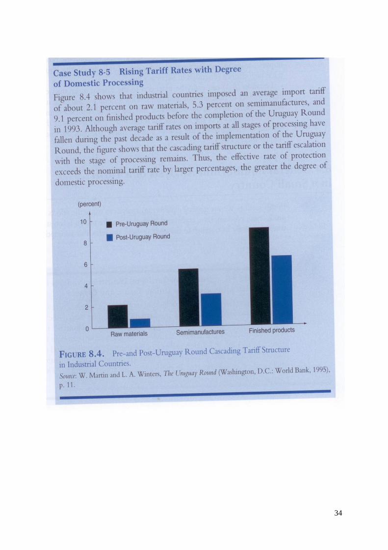
Furthermore, most industrial nations have a ‘cascading’ tariff structure with very low
or zero nominal tariffs on raw materials and higher and higher rates the greater is the
degree of processing.
The highest rates of effective protection in industrial nations are often found
on simple labor-intensive commodities, such as textiles, in which developing
countries have a comparative advantage.
(Read and discuss case study 8-5, page 34)
B- The Optimum Tariff
When a large nation imposes an import tariff, its volume of trade decreases, but the
nation’s terms of trade improve.
The optimum tariff is one that maximizes the net benefit resulting from improvement
in the nation’s terms of trade against the negative effect resulting from reduction in the
volume of trade.
However, since the nation’s benefit comes at the expense of other nations, the latter are
likely to retaliate. In the end, all nations usually lose.

33
34

35
Chapter Three ECONOMIC INTEGRATION
3.1 Introduction:
In this chapter, we examine ‘economic integration’ in general and ‘customs unions’
in particular.
The theory of economic integration refers to the commercial policy of discriminatively
reducing or eliminating trade barriers only among the nations joining together.
There are various degrees of economic integrations ranging from preferential trade
arrangements to economic unions.
After definitions of the types of economic integrations, we’ll explain the effects of
custom unions, and the theory of second best.
3.2 Degrees (types) of Economic Integrations:
a) Preferential Trade Arrangements:
This type of integrations provides lower barriers on trade among participating nations
than on trade with nonmember nations.
This is the loosest form of economic integration.
The best example of this type is the ‘British Commonwealth Preference
System’.
(It was established in 1932 by the United Kingdom with members and some
former members of British Empire. (for detail, see (http://tr.wikipedia.org)-
İngiliz Milletler Topluluğu.)
b) Free Trade Area:
It is the form of economic integration wherein all barriers are removed on trade
among members, but each nation retains its own barriers to trade with nonmembers.
The best examples are :
European Free Trade Association (EFTA)
Formed in 1960.
By the United Kingdom, Austria, Denmark, Norway, Portugal,
Sweden and Switzerland (with Finland joining as associate
member in 1961)
The North American Free Trade Agreement (NAFTA)
Formed in 1993 by the United States, Canada, and Mexico.

36
c) Customs Union:
A customs union allows no tariffs or other barriers on trade among members (as in
a free trade area), and in addition it harmonizes trade policies (such as the setting of common
tariff rates) toward the rest of the world.
The most famous example is the ‘European Union (EU)’, or ‘European
Common Market’.
Formed in 1957.
By West Germany, France, Italy, Belgium, the Netherlands,
Luxembourg. (Now, 27 members)
d) Common Market:
A common market goes beyond a customs union by also allowing the free
movement of labor and capital among member nations.
Example: The European Union (EU) achieved the status of a common market
at the beginning of 1993.
e) Economic Union:
It goes still further by ‘harmonizing or even ‘unifying’ the monetary and fiscal
policies of member states.
This is the most advanced type of economic integration.
An example of ‘complete economic and monetary union’ is the United States.
Benelux is another example (formed by Belgium, the Netherlands, and
Luxembourg after World War II and now part of the EU).
The European Union has made strides in forming an economic union to a great
extent.
f) Duty-free Zones (or free economic zones):
There are areas set up to attract foreign investments by allowing raw materials and
intermediate products duty free.
Such areas can be set up in different locations of a country.

37
3.3 Trade Creating and Trade Diverting Effects of a Customs Union
A customs union results in two opposite effects: trade creation and trade diversion.
The net effect on the world welfare is measured by comparing of these two effects.
A. Trade Creation:
Trade creation occurs when some domestic production in a member nation is
replaced by lower-cost imports from another member nation.
This increases the welfare of member nations because it leads to greater
specialization in production based on comparative advantage (assuming that all
economic resources are fully employed before and after formation of the
customs union.)
A trade-creating customs union also increases the welfare of nonmembers
because some of the increase in its real income spills over into increased
imports from the rest of the world.
Illustration of a trade creating customs union:
Suppose that there are only three nations in the world.
The commodity produced and traded is X.
Nation 1 can produce commodity X at a cost of $1.
Nation 2 can produce commodity X at a cost of $3.
Nation 3 can produce commodity X at a cost of $1,5.
Nation 2 initially imposes a nondiscriminatory ad valorem tariff of
100 percent on the imports of commodity X.
In this case, only Nation 1, whose price also represents the world
price, can sell commodity X to Nation 2 at Px=$2, as shown in figure
3.1.

38
Figure 3.1 Nation 2
Nation 2 does not import commodity X from Nation 3 because the tariff-inclusive
price of commodity X imported from Nation 3 would be PX = $3.
Now, Nation 2 forms a customs union with Nation 1.That is, Nation 2
removes tariffs on its imports from Nation 1 only.
Then, PX=$1 in Nation 2.
In this case,
Nation 2 consumes 70X (AB) of commodity X.
Nation 2 produces 10X domestically.
Nation 2 imports 60X from Nation 1.
Nation 2 collects no tariff revenue.
The benefit to consumers in Nation 2 (resulting from the formation of the
customs union) is equal to AGHB. (i.e. increase in consumer surplus).
However, only part of this represents a net gain for Nation 2 as a whole.
Because,
AGJC represents a reduction in producer surplus.
MJHN represents the loss of tariff revenues.
Nation 1’s
price + tariff S1+T
A 1
2
3
4
5
0 10 20 30 40 50 60 70
B C
C
E
H G
M
J
N S1
DX
SX
PX($)
X (unit)
Nation 1’s
price
(5)
(15)
(10)
(30)

39
In this case, the net gain for Nation 2 equals:
[Increase in consumer surplus (AGHB)] - [reduction in producer surplus (AGJC)] + [the loss
of tariff revenues (MJHN)]
That is, it is equal to ‘CJM’ + ‘BHM’. Here, ‘CJM’ refers to the production
effect and ‘BHM’ refers to the consumption effect.
As you can recall, the sum of the areas of shaded triangles (CJM+BHN)
represents deadweight loss in case of tariff imposition.
In other words, deadweight loss before customs union becomes net gain for the
importing nation afterwards.
B. Trade Diversion:
Trade diversion occurs when lower-cost imports from outside the customs union are
replaced by higher-cost imports from a union member.
Trade diversion reduces welfare because it shifts production from more efficient
producers outside the customs union to less efficient producers inside the union.
Thus, trade diversion worsens the international allocation of resources and shifts
production away from comparative advantage.
A trade diverting customs union results in both
Trade creation and
Trade diversion
And therefore can increase or reduce the welfare of union members, depending on
relative strength of these two opposing forces.
40
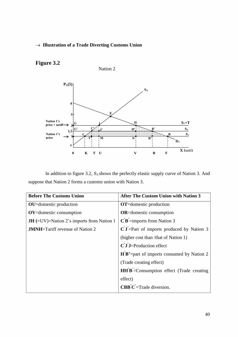
Illustration of a Trade Diverting Customs Union
Figure 3.2 Nation 2
In addition to figure 3.2, S3 shows the perfectly elastic supply curve of Nation 3. And
suppose that Nation 2 forms a customs union with Nation 3.
Before The Customs Union After The Custom Union with Nation 3
OU=domestic production OT=domestic production
OV=domestic consumption OR=domestic consumption
JH (=UV)=Nation 2’s imports from Nation 1 C’B
’=imports from Nation 3
JMNH=Tariff revenue of Nation 2
C’J
’=Part of imports produced by Nation 3
(higher cost than /that of Nation 1)
C’J
’J=Production effect
H’B’=part of imports consumed by Nation 2
(Trade creating effect)
HH’B
’=Consumption effect (Trade creating
effect)
CBB’C
’=Trade diversion.
T’
C
C
C’
Nation 1’s
price + tariff S1+T
G’
1
2
3
4
0 K T U V R F
B
E
H G
M
J
N
S1
DX
SX
PX($)
X (unit)
Nation 1’s
price
J’ H’
R’
B’ S3 1,5
z

41
Of this trade diversion,
CT’C
’=deadweight loss resulting from production.
BR’B
’=deadweight loss resulting from consumption.
C’T
’R
’B
’=welfare loss resulting from higher- costs production
than that of Nation 1.
So, C’J
’J + HH
’B
’ is compared to CBB
’C’ to measure the net effect of the customs
union.
If C’J
’J + HH
’B’ > CBB
’C
’, then net effect is positive.
If C’J
’J + HH
’B’< CBB
’C
’, then net effect is negative.
The several attempts to measure the static welfare effects resulting from the formation
of the European Union all came up with surprisingly small ‘net static’ welfare gains.
C. Dynamic Benefits from a Customs Union
Beside the static welfare effects discussed above, the nations forming a customs union
are likely to receive several important ‘dynamic’ benefits.
These are due to:
Increased competition
Economies of scale
Stimulus to investment, and
Better utilization of economic resources.

42
Chapter Four SPECIFIC TRADE REGIMES
4.1 Introduction → Goods imported by a nation are, as a rule, subject to the import regime of the nation, and
the tariffs are paid for them according to the customs tariff schedule.
→ However, some foreign trade transactions, because of their specifications, are realized
without being subject to normal customs procedures of the country.
In this chapter, these specific customs regimes will be explained briefly.
4.2 Temporary Imports and Temporary Exports 4.2a Temporary Imports (Inward processing regime): Temporary imports regime are
applied for the goods which are imported with the condition that they will be taken out of the
country after a certain time. Under this regime, imported goods are not subject to tariffs.
Examples:
- Overseas goods that will be repaired or improved.
- Construction equipment and machinery lease from abroad.
- Goods brought into the country from a foreign country for fairs and
demonstrations.
- Tools brought by circus and theatrical companies.
- Model products, packages, films and like.
4.2b Temporary Exports (Outward processing regime): As opposed to temporary
imports, under this regime, the goods that are exported are brought into the home country
after a certain time.
For example: Bringing back of mineral ore which is exported in order to be melted.

43
4.3 Free Zones
→ Free zones are the areas set up within the national borders but regarded outside the
customs area.
→ Legal and administrative rules in effect of the country are either not applied or applied to a
certain extend in these areas (free zones).
→ Types of free zones:
Free Trade Zones: This type of free zones is set up rather for
commercial purposes. Goods stored in these zones are sent to
importing countries later on.
Free Production Zones: This type of zones is set up for the
production and assembling (montage) of light products. These
zones are sometimes called “export processing zones” because
the aim is to attract foreign investments by allowing raw
materials and intermediate products duty-free, thereby to
increase exports.
Free Ports: These zones are set up in the main arteries of
commerce for the commercial activities such as export, import,
re-export and transit trade.
Free ports are critically important for landlocked countries in
order to stand out to ocean trade roads.
→ Why free zones to establish:
In short,
1. To produce with lower costs benefiting from incentives and advantages provided by the
home country, and thereby to increase the exports.
2. To attract foreign investments and technologies.
3. To obtain raw materials and intermediate goods in time and easily.
44
4. To ease the “transit merchandise trade”.
5. To raise employment level.
6. To increase foreign currency inflow.
→ In Turkey,
The first free zones were established in Mersin and Antalya in
1987. There are 19 free zones (2010). There were 21 in 2009.
Total trade volume was $ 24.5 billion in 2007 and $ 18.5 billion
in 2010.
Of this volume, more than 30 percent are exported to European
Union countries.
Total employment is 48 684 people (2010).
4.4 Warehouses (Entrepot, Storehouse)
→ Warehouses are closed spaces where goods are stored under the customs authority for a
long time.
→ There is no tariff payment for these goods as long as they are stored in the warehouse. The
goods are subject to customs duty when they are imported by the host country.
→ Warehouses provide many facilities for road trade (as well as free zones for maritime
trade).
- The buyers (importers) can see the goods on-site, and have a chance to import in
parts.
- The sellers (exporters), on the other side, have a chance to wait for selling their
goods at favorable prices.
- The importers do not have to pay all customs duties in one go when they import in
parts.
45
4.5 Transit Transportation
→ Transit transportation means that goods sent from one country to another are gone through
the borders of a third country.
→ Today , the main principle in transit transportation is “the right of free entry”.
→ Among the multilateral agreements regulating transit transportations, TIR Agreement
(Transit International Routier) of 1959 holds the first place.
Transit transportation is sometimes confused with “transit merchandise trade.”
Reexport, exportation and importation from free zones are regarded as transit
merchandise trade.
Transit merchandise trade is benefited from export incentives as well as exports of
other goods and services.
4.6 Border and Coastal Trade
It is a type of trade that a nation trades with the nations they have common land and
sea frontiers, which is subject to a specific regime.
The aim of border and coastal trade is to meet the needs of people living on both sides
of the frontiers.
In this type of trade, import and export certificates are not needed. Also, there is no
need for “bill of entry” and “certificate of clearance outward.”
4.7 Unpaid Non-Quota Imports (Unpaid Importations)
Unpaid importation includes imports of some personal and non-traded goods bought
by income that is earned abroad, and with no transfer of foreign exchange from the
country.
In this type of importation, only custom duty is not paid; but,
other taxes such as value added and private consumption taxes are levied.