international supply chains and trade elasticity in times ... · staff working paper ersd-2010-08...

Staff Working Paper ERSD-2010-08 Date: February 2010

World Trade Organization Economic Research and Statistics Division

International Supply Chains and Trade Elasticity in Times of Global Crisis

Hubert Escaith: Economic Research and Statistics, WTO

Nannette Lindenberg: Institute of Empirical Economic Research, University of Osnabrück

Sébastien Miroudot: Trade and Agriculture Directorate, Trade Policy Linkages and Services Division, OECD

Manuscript date: 1 February 2010

Acknowledgements: The authors thank Christophe Degain and Andreas Maurer for their suggestions and cooperation during the preparation of this research, and IDE-Jetro for providing the Asian Input-Output tables. The views expressed in this document, which has not been submitted to formal editing, are those of the authors and do not represent a position, official or unofficial, of the OECD, the WTO Secretariat or WTO Members and OECD Member countries. Disclaimer: This is a working paper, and hence it represents research in progress. This paper represents the opinions of the authors, and is the product of professional research. It is not meant to represent the position or opinions of the WTO or its Members, nor the official position of any staff members. Any errors are the fault of the authors. Copies of working papers can be requested from the divisional secretariat by writing to: Economic Research and Statistics Division, World Trade Organization, Rue de Lausanne 154, CH 1211 Geneva 21, Switzerland. Please request papers by number and title.

International Supply Chains and Trade Elasticity

in Times of Global Crisis Abstract: The paper investigates the role of global supply chains in explaining the trade collapse of 2008-2009 and the long-term variations observed in trade elasticity. Building on the empirical results obtained from a subset of input-output matrices and the exploratory analysis of a large and diversified sample of countries, a formal model is specified to measure the respective short-term and long-term dynamics of trade elasticity. The model is then used to formally probe the role of vertical integration in explaining changes in trade elasticity. Aggregated results on long-term trade elasticity tend to support the hypothesis that world economy has undertaken in the late 1980s a "traverse" between two underlying economic models. During this transition, the expansion of international supply chains determined an apparent increase in trade elasticity. Two supply chains related effects (the composition and the bullwhip effects) explain also the overshooting of trade elasticity that occurred during the 2008-2009 trade collapse. But vertical specialization is unable to explain the heterogeneity observed on a country and sectoral level, indicating that other contributive factors may also have been at work to explain the diversity of the observed results. Keywords: international supply chain, trade elasticity, global crisis, trade collapse, input-output analysis, error-correction-model JEL: C67, F15, F19

- 1 -

INTRODUCTION The crisis that, after several months of gestation in the US financial sphere, irrupted into the international scene in September 2008 has been dubbed the "Great Trade Collapse" for its impact on international commerce. The shock, emanating from the largest world financial centre, spread very quickly and almost simultaneously to most industrial and emerging countries. The collapse of world trade has been unprecedented, even in comparison with the Great Depression of the 1930s (Eichengreen and O’Rourke, 2009). During the first quarter of 2009, world exports in value terms were 31 percent lower than one year before and world imports 30 percent lower. Also significant is the fact that freight rates for containers shipped from Asia to Europe have reached zero in the middle of January 2009 for the first time in history. International trade, which dropped five times more rapidly than global GDP, was both a casualty of the 2008-2009 crisis and one of its main channels of transmission. While a decrease in trade is expected when world output falls following a severe financial crisis, the magnitude of the collapse has surprised observers. This overreaction is reflected in high trade elasticities. Moreover, the trade collapse was not only sudden and severe, but also synchronized, which is another distinguishing feature of the current crisis. One prominent and often discussed new element in world production is the emergence of global supply chains. The recent phase of globalization, to be identified with the emblematic 1989 year, saw the emergence of new business models that built on new opportunities to develop comparative advantages (Krugman, 1995; Baldwin, 2006).1 With the opening of new markets, the technical revolution in IT and communications, and the closer harmonization of economic models worldwide, trade became much more than just a simple exchange of merchandise across borders. It developed into a constant flow of investment, of technologies and technicians, of goods for processing and business services, in what has been called the "Global Supply Chain". While providing renewed opportunities for increasing productivity and promoting industrialization in developing countries, the greater industrial interconnection of the global economy has created newer and faster channels for the propagation of adverse external shocks. Referring to the breakdown of 2008-2009, some authors have pointed out that they may explain the abrupt decrease in trade or the synchronization of the trade collapse. The question is of importance for its economic and financial implications, but also for its social impact as the reorganization of global supply chains implies the destruction and creation of jobs at different locations. But has the impressive collapse in world trade really been caused by global supply chains? If the answer is yes, we should expect a deeper decrease of trade in those countries and sectors that participate in global production networks and a smoother reaction in those that produce mainly for the domestic market. Moreover, we should also expect that global supply chains play a role in the synchronization of the trade collapse and its size. One reason for this is the inherent magnification effect of global production networks: intermediate inputs cross the border several times before the final product is shipped to the final costumer. All the different production stages of the global supply chain rely on each other – as suppliers and as customers. Thus, if a shock occurs in one of the participating sectors or countries, the shock is transmitted quickly to the other stages of the supply chain through both backward and forward linkages. These transmission channels apply both to financial shocks, e.g. a credit crunch in

1 1989 is known for the fall of the Berlin Wall, which brought down the barriers that had split the post-

WWII world; it should also be reminded for the Brady Bonds, which put an end to the decade-long debt crisis that plagued many developing countries. In continuation, the 1990s saw the conclusion of the Uruguay Round and the birth of the WTO, which brought down many trade barriers and led to further liberalization in areas like telecommunications, financial services and information technologies.

- 2 -

one country, and to trade policy shocks, e.g. rising tariffs and non-tariff barriers, or implementing "buying local” campaigns. Another explanation of why trade has been affected harder than GDP is the composition effect. Trade flows are composed mainly of durable goods (about two thirds or more), while GDP consists mainly of services. Trade in goods was strongly impacted by the crisis while services showed some resilience to the crisis (Borchert and Mattoo, 2009). Lastly, there is an accounting bias, as GDP is measured as value-added and trade in gross values. The reminder of the paper is organized as follows. The first section gives a brief overview of the related literature. The next section identifies stylized facts on vertical integration and trade multipliers compiled from international input-output statistics. Section three extends the exploration of trade data patterns by estimating import multipliers for a larger selection of countries, regions and sectors. Section four develops a formal dynamic model incorporating short-run and long-term components. The last section concludes and provides the main policy implications of the analysis. I. A BRIEF REVIEW OF THE LITERATURE

Trade in tasks and the fragmentation of production along global supply chains has challenged the validity of the traditional Ricardian models, based on the exchange of final goods, each country specializing in a certain type of products. Contrary to the Ricardian model, countries that are similar in factor endowment and technology have developed a significant part of their trade in the same products, and trade intermediate goods between their industries (Box 1). The new trade theory, by introducing imperfect competition, consumer preference for variety and economies of scale, looks at explaining divergence from this traditional model. An early appraisal of the extent of outsourcing can be found in Feenstra (1998) who compares several measures of outsourcing and argues that all have risen since the 1970s. Always on the descriptive side, Agnese and Ricart (2009) provide details on the extent of offshoring during 1995-2000 for several countries throughout the world and show that offshoring is not only a phenomenon among large developed economies. Besides, the authors provide evidence that offshoring is much more prominent in the manufacturing sector. 2 An illustrative example of a globalized supply chain can be found in Linden et al. (2007), who study the case of Apple's iPod. Hanson et al. (2005) conduct a firm-level analysis with US multinationals and analyze the driving forces of inter-firm trade in intermediate inputs. Paul and Wooster (2008) study the financial characteristics of outsourcer firms in the US; they find that compared to non-outsourcing firms the former have higher costs and lower profitability and have to perform in more competitive industries. Coucke and Sleuwaegen (2008), who analyze a firm data set of the Belgian manufacturing sector, argue that firms that engage in offshoring activities improve their chances of survival in a globalizing industry. Nordås (2005) gives a review of vertical specialization and presents six country case studies, namely of Brazil, China, Germany, Japan, South Africa and the USA, analyzing production sharing in the automotive and the electronics industry. Sturgeon and Gereffi (2009) contribute to the understanding of the phenomenon from a business perspective, providing an overview of the micro-economic evidence and the role of outsourcing in industrial upgrading and competitiveness, while pointing-out some crucial data issues. On the conceptual side, the critic of the traditional Ricardian hypotheses and the development of new concepts have led to a vast literature (see Helpman, 2006 and WTO, 2008a for a review). We will focus on a few articles that have a direct relation to our analysis.

2 Although service offshoring has been rising significantly in recent years, it still accounts only for a small fraction of total offshoring; see OECD (2008) for an overview.

- 3 -

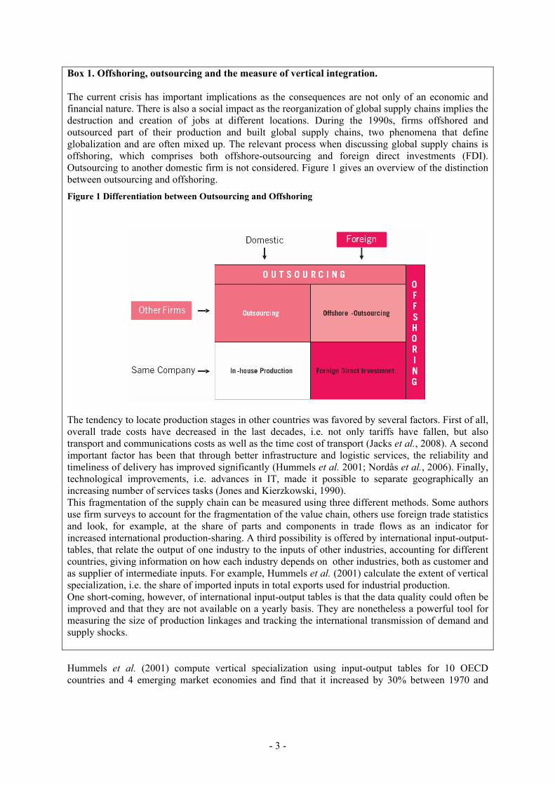
Box 1. Offshoring, outsourcing and the measure of vertical integration. The current crisis has important implications as the consequences are not only of an economic and financial nature. There is also a social impact as the reorganization of global supply chains implies the destruction and creation of jobs at different locations. During the 1990s, firms offshored and outsourced part of their production and built global supply chains, two phenomena that define globalization and are often mixed up. The relevant process when discussing global supply chains is offshoring, which comprises both offshore-outsourcing and foreign direct investments (FDI). Outsourcing to another domestic firm is not considered. Figure 1 gives an overview of the distinction between outsourcing and offshoring. Figure 1 Differentiation between Outsourcing and Offshoring

The tendency to locate production stages in other countries was favored by several factors. First of all, overall trade costs have decreased in the last decades, i.e. not only tariffs have fallen, but also transport and communications costs as well as the time cost of transport (Jacks et al., 2008). A second important factor has been that through better infrastructure and logistic services, the reliability and timeliness of delivery has improved significantly (Hummels et al. 2001; Nordås et al., 2006). Finally, technological improvements, i.e. advances in IT, made it possible to separate geographically an increasing number of services tasks (Jones and Kierzkowski, 1990). This fragmentation of the supply chain can be measured using three different methods. Some authors use firm surveys to account for the fragmentation of the value chain, others use foreign trade statistics and look, for example, at the share of parts and components in trade flows as an indicator for increased international production-sharing. A third possibility is offered by international input-output-tables, that relate the output of one industry to the inputs of other industries, accounting for different countries, giving information on how each industry depends on other industries, both as customer and as supplier of intermediate inputs. For example, Hummels et al. (2001) calculate the extent of vertical specialization, i.e. the share of imported inputs in total exports used for industrial production. One short-coming, however, of international input-output tables is that the data quality could often be improved and that they are not available on a yearly basis. They are nonetheless a powerful tool for measuring the size of production linkages and tracking the international transmission of demand and supply shocks. Hummels et al. (2001) compute vertical specialization using input-output tables for 10 OECD countries and 4 emerging market economies and find that it increased by 30% between 1970 and

- 4 -

1990.3 Yi (2003) builds on these findings and proposes a dynamic Ricardian trade model of vertical specialization that can explain the bulk of the growth of trade. A stock-taking of offshore outsourcing and the way it is perceived by economists and non-economists is made in Mankiw and Swagel (2006). A straightforward introduction to the economics of offshoring, the underlying motivations and effects is given in Smith (2006). Grossman and Rossi-Hansberg (2008) present a model of offshoring where the production process is represented as a continuum of tasks. The authors, thus, focus on tradable tasks rather than on trade of finished goods, i.e. during the production process, different countries participate in global supply chains by adding value. Yet another model of offshoring is proposed by Harms et al. (2009) who allow for variations of the cost saving potential along the production chain and consider transportation costs for unfinished goods. Within this framework they can explain large changes in offshoring activities with small variations of the parameters of their model. The link between the offshoring literature and the research on firm heterogeneity is established in Mitra and Ranjan (2008). They construct an offshoring model with firm heterogeneity and externalities and study the effects of temporary shocks on offshoring activities. Grossman and Helpman (2005) develop a model to study outsourcing decisions focusing on equilibria where some firms outsource in the home country and others abroad. In an earlier paper (Grossman and Helpman, 2002) the authors propose a general equilibrium model of the "make-or-buy-decision", i.e. the decision between insourcing and outsourcing. A model that allows firms to choose between vertical integration and outsourcing, as well as between locating the production at home or in the low-wage South is proposed by Antràs and Helpman (2004). They point out that the more productive firms source inputs in low-cost countries whereas less productive firms in the high-cost countries of the North. Besides, if both types of firms acquire inputs in the same country, the former insource and the latter outsource. An explanation for the steady increase in outsourcing activities is offered by Şener and Zhao (2009), who analyze the globalization process by setting up a dynamic model of trade with endogenous innovation, where a local-sourcing-targeted and an outsourcing-targeted R&D race take place at the same time. The latter represents the so called "iPod cycle" where firms combine innovation activity with simultaneous outsourcing, a form of R&D strategy which becomes more and more important. Ornelas and Turner (2008) propose another model that explains the current trend towards foreign outsourcing and intra-firm trade. That the motivation for outsourcing can also be strategic rather than cost-motivated is shown by Chen et al. (2004). They model strategic outsourcing as a response to trade liberalization in the intermediate-product market. Of particular relevance for the present analysis, various papers help to understand the volatility linked to globalized activities. Du et al. (2009) elaborate a model on bi-sourcing, i.e. simultaneous outsourcing and insourcing for the same set of inputs, a strategy that is more and more often adopted by multinational enterprises. The use of this strategy, with the inherent options of preferring either the external or the internal source of intermediate inputs, may explain part of the reduction of trade flows in times of economic crisis. A model of in-house competition, i.e. between the different facilities of a multiplant firm, is introduced by Kerschbamer and Tournas (2003). Their model shows that in downturns firms may decide to produce in the establishment that has higher costs even when it would also be possible to locate production to the lower cost facility. The stability of supply chain networks is studied in Ostrovsky (2008), who proposes a model of matching in supply chains. The author deduces the sufficient conditions for the existence of stable networks which, however, rely on the assumptions of the model of same-side substitutability and cross-side complementarity. Bergin et al. (2009) analyze empirically the volatility of the Mexican export-processing industry compared to their US

3 An update for 2005 and 40 countries is provided in Miroudot and Ragoussis (2009). An alternative methodology based on international I/O tables can be found in Inomata (2008).

- 5 -

counterparts with a difference-in-difference approach; they find that, on average, the fluctuations in value added in the Mexican outsourcing industries are twice as high as in the US. In addition, the authors propose a theoretical model of outsourcing that can explain this stylized fact. Box 2. Trade Elasticities. Elasticities measure the responsiveness of demand or supply to changes in income, prices, or other variables. Two prominent representatives of elasticities are the income elasticity and the price elasticity of demand. While the former measures the percentage change in the quantity demanded resulting from a one-percent increase in income, the latter measures the percentage change in the quantity demanded resulting from a change of one percent in its price.

IQ

QI

IIQQEand

PQ

QP

PPQQE IP Δ

Δ=

ΔΔ

=ΔΔ

=ΔΔ

=//

// ,

with E = elasticity, Q = quantity demanded, P = price, and I = income.

In consumer theory, price elasticity is complemented by elasticity of substitution between competing goods and services, leading to the concept of indifference curves. In this paper we will focus on the macro-economic income elasticities of trade, in short, trade elasticities.

It is important to remember that in most of the literature reviewed in this paper, neither price effects nor substitutions effects are explicitly taken into consideration in this context. Thus, the trade elasticities are reflecting the pure effect of a change in domestic income (measured by GDP) to the quantity of imports. It is also the convention that we will adopt in the rest of the paper.

The variation in the relative price of exports and imports is, nonetheless, implicitly taken into consideration in the calculation of the domestic product. Because GDP, on the demand side, is equal to the sum of consumption, investment and the net balance between exports minus imports (X-M), any changes in the terms of trade that affect (X-M) will be reflected, ceteris paribus, into the domestic product. The terms of trade effect is immediate when GDP is computed at current prices; it is formally imputed by national accounts when elaborated at constant prices.

Finally, Tanaka (2009) and Yi (2009), among others, explain the collapse of trade during the current world wide crisis as a systematic over-shooting due to the globalization of supply chains. However, Bénassy-Quéré et al. (2009), using a multi-region/multi-sector CGE model, reject this hypothesis. Freund (2009) analyzes the effect of a global downturn on trade with a historical perspective. She finds that the elasticity of trade to GDP (see Box 2) has increased significantly in the last 50 years and that in times of crisis trade is even more responsive to GDP. McKibbin and Stoeckel (2009) point out that the distinction between durable and non durable goods is fundamental to explain the overreaction of trade to the contraction of GDP in the current crisis. Borchert and Mattoo (2009) emphasize that services trade is much less affected in the crisis than goods trade. They argue that this can probably be explained by lower demand cyclicality and less dependence on external finance. Escaith and Gonguet (2009) study the transmission of financial shocks by international supply chains and propose an indicator of supply-driven shocks. A series of studies in Inomata and Uchida (2009) look at the various dimensions (trade, employment, finance) of the global crisis in the Asian Pacific region. II. STYLIZED FACTS AND TRADE MULTIPLIERS FROM AN INPUT-OUTPUT

PERSPECTIVE

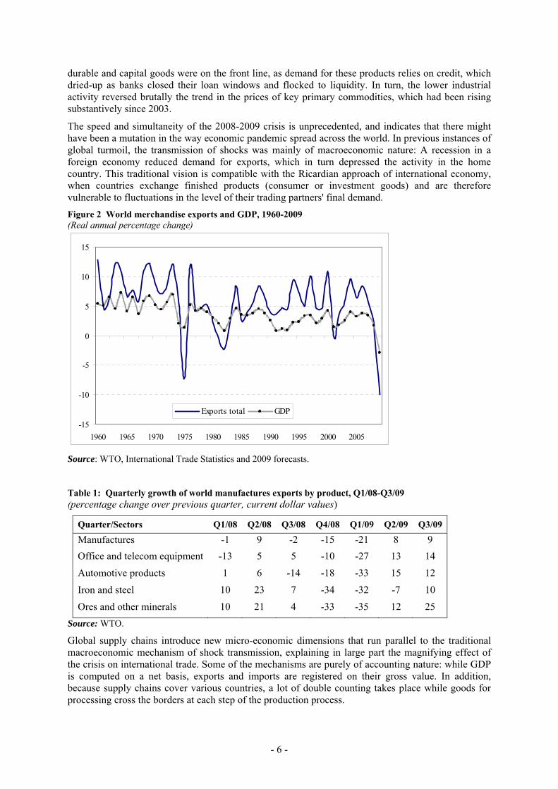
As mentioned in the introduction, trade reacted very strongly to the first signals of recession in 2008 (Figure 2). The sectors most affected were fuels and minerals, due to a strong price effect, and machinery and transport equipment because of a strong demand effect (Table 1). Indeed, consumer

- 6 -

durable and capital goods were on the front line, as demand for these products relies on credit, which dried-up as banks closed their loan windows and flocked to liquidity. In turn, the lower industrial activity reversed brutally the trend in the prices of key primary commodities, which had been rising substantively since 2003.

The speed and simultaneity of the 2008-2009 crisis is unprecedented, and indicates that there might have been a mutation in the way economic pandemic spread across the world. In previous instances of global turmoil, the transmission of shocks was mainly of macroeconomic nature: A recession in a foreign economy reduced demand for exports, which in turn depressed the activity in the home country. This traditional vision is compatible with the Ricardian approach of international economy, when countries exchange finished products (consumer or investment goods) and are therefore vulnerable to fluctuations in the level of their trading partners' final demand. Figure 2 World merchandise exports and GDP, 1960-2009 (Real annual percentage change)

-15

-10

-5

0

5

10

15

1960 1965 1970 1975 1980 1985 1990 1995 2000 2005

Exports total GDP

Source: WTO, International Trade Statistics and 2009 forecasts.

Table 1: Quarterly growth of world manufactures exports by product, Q1/08-Q3/09 (percentage change over previous quarter, current dollar values)

Quarter/Sectors Q1/08 Q2/08 Q3/08 Q4/08 Q1/09 Q2/09 Q3/09

Manufactures -1 9 -2 -15 -21 8 9 Office and telecom equipment -13 5 5 -10 -27 13 14 Automotive products 1 6 -14 -18 -33 15 12 Iron and steel 10 23 7 -34 -32 -7 10 Ores and other minerals 10 21 4 -33 -35 12 25

Source: WTO.

Global supply chains introduce new micro-economic dimensions that run parallel to the traditional macroeconomic mechanism of shock transmission, explaining in large part the magnifying effect of the crisis on international trade. Some of the mechanisms are purely of accounting nature: while GDP is computed on a net basis, exports and imports are registered on their gross value. In addition, because supply chains cover various countries, a lot of double counting takes place while goods for processing cross the borders at each step of the production process.

- 7 -

But the core of the explanation is to be found in the economic implications of the structural changes that affected world production since the late 1980s. In the contemporaneous context, adverse external shocks affect firms not only through their sales of finished goods (the final demand of national accounts), but also through fluctuations in the supply and demand of intermediate inputs. It has therefore been tempting to attribute the large trade-GDP elasticity, close to 5 in 2009, to the leverage effect induced by this geographical fragmentation of production.

• Vertical integration and trade magnifier

In the following section, we focus on the USA and Asia, a sub-set that epitomizes the vertical integration phenomenon from both a micro and macro perspective. The investigation, based on observed data, relies on national accounts and statistics on inter-sectoral trade in inputs produced by IDE-Jetro for various benchmark years.4 The information is presented as a set of interlinked input-output tables to form an estimate of the composition of intermediate and final flows of goods and services between home and foreign countries. The calculation of a "Leontief inverse matrix" derived from these IO matrices is used to estimate the resulting effect of the series of direct and indirect effects on all domestic sectors of activity. This procedure allows to estimate the imported content of exports and to measure the vertical integration of productive sectors.

As seen in Table 2, the observations on the USA and Asia, one of the most dynamic trade compact in the recent history of international trade, tend to support the "magnifying hypothesis". While exports of final products (consumer and investment goods) increased 7% in annual average over the 1990-2008 period, exports of inputs (intermediate consumption, in the national account terminology) raised by more than 10% per year. In the same time, imports of such intermediate goods increased by 9%.5 Table 2: Asia and the USA: Annual growth of intermediate inputs and exports, 1990-2008

Exports

Total Imported intermediates Intermediate inputs Final goods and services Total

Agriculture 9.5 3.5 13.0 5.9 Mining quarrying 15.6 7.6 ... 7.9

Manufacturing 9.0 10.7 6.6 9.1 Total sectors 9.1 10.2 7.1 9.1

Note: Sum of China, Indonesia, Japan, Korea, Malaysia, Taipei, Philippines, Singapore, Thailand, and the USA in nominal values in US dollar; Total sectors include services and other sectors; 2008 estimates. Imports and exports include exchanges with the rest of the world. Source: Authors calculation, based on IDE-Jetro Asian Input-Output matrices. Because intermediate goods include commodities, in particular fuels, and are valuated at nominal prices, imports of intermediate goods show the highest growth rate for mining and quarrying. But manufacturing is the sector where exports of intermediate products increased most since 1990, comforting the hypothesis that vertical integration and trade in intermediate goods drove international trade in the recent past, and explained the trade collapse after September 2008.

Retrospectively, there is a clear signal that export-led growth among developing economies has been associated with higher reliance on imported inputs. To mention a recent study on production sharing and the value added content of trade (Johnson and Noguera, 2009), countries systematically shift towards manufacturing exports, which have lower value added content on average, as they grow richer and this depresses the aggregate value added to export ratio per unit value.6 These authors show

4 We used the 7 sectors aggregation for 1990, 1995, 2000 and 2008 matrices. The data for 2008 are estimates, other years are derived from national accounts and countries' official statistics. For a presentation and evaluation, see IDE-Jetro (2006), Oosterhaven, Stelder and Inomata (2007), and Inomata and Uchida (2009).

5 Differences between imports and exports are due to the rest of the world (ROW). Within an international IO, trade is symmetric (bilateral exports should equal bilateral imports).

6 Obviously, this strategy of diversifying into manufacture allows the developing countries to increase labour productivity and generate more income per capita. Thus richer countries are not defined by the intensity of the creation of value added, but by its extension.

- 8 -

that the largest exporters among developed countries (Germany and USA) see their value added content scaled down due to a more integrated production structure with their respective regional partners (NAFTA for the US, and EU for Germany).

These findings support the claim that supply chains and the fragmentation of manufacture production explain the over-shooting of trade elasticity during the crisis (Tanaka, 2009; Yi, 2009). Other experts, nevertheless, contest the hypothesis that higher demand elasticity behind the Great Trade Collapse could have been caused by vertical integration (Bénassy-Quéré et al., 2009) because it affects only the relative volume of trade in relation to GDP (levels), while elasticity should remain constant in a general equilibrium context.

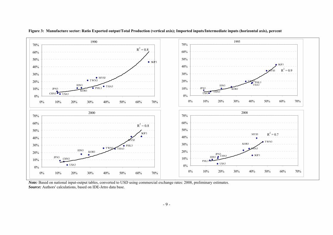
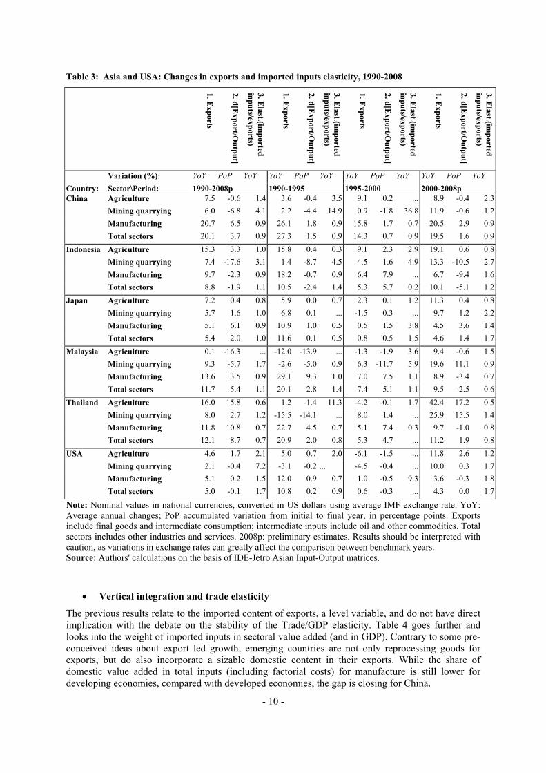
The data compiled from national accounts data on Asian economies and the USA since 1990 (Table 3) confirms the positive relationship between export orientation (share of export over total output) and reliance on imported inputs. Figure 3 shows that the relationship is rather stable over time between 1990 and 2000, at least on manufactured products where it is stronger than for other product groups. 7 Table 3 indicates also that all the Asian economies increased their exposure to exports during the 1990-2008 period while the USA registered a slight reduction, especially before 2000.

The ratio of imported inputs in relation to total exports (all sectors together) is stable for most economies (aggregated results for column 3 –growth rate of imported inputs / growth rate of exports– are close to 1). The exceptions are the USA and Japan where elasticity is about 1.7 percentage points (i.e., an increase in 1 percentage point of exports necessitates a 1.7% increase in imported inputs). Considering the size of these economies, this would indicate that the increase in the weight of intermediate goods in world trade is the result of the change in business models in developed economies, rather than due to the emergence of developing countries. Moreover, the latter may both result and explain the former, as the recent industrialization phase of developing countries is closely linked to the outsourcing strategy of transnational corporations (Sturgeon and Gereffi, 2009).

7 The data for 2008 tend to indicate a reduction in the reliance on imported inputs. Yet, because the

2008 data are based on estimates rather than official national account statistics, this result should be taken with care.

- 9 -

Figure 3: Manufacture sector: Ratio Exported output/Total Production (vertical axis); Imported inputs/Intermediate inputs (horizontal axis), percent

Note: Based on national input-output tables, converted to USD using commercial exchange rates: 2008, preliminary estimates. Source: Authors' calculations, based on IDE-Jetro data base.

CHN3

IDN3JPN3

KOR3

MYS3TWN3

PHL3

SGP3

THA3

USA3

R2 = 0.8

0%

10%

20%

30%

40%

50%

60%

70%

0% 10% 20% 30% 40% 50% 60% 70%

1990

CHN3

IDN3JPN3 KOR3

MYS3

TWN3PHL3

SGP3

THA3

USA3

R2 = 0.9

0%

10%

20%

30%

40%

50%

60%

70%

0% 10% 20% 30% 40% 50% 60% 70%

1995

USA3

THA3

SGP3

PHL3TWN3

MYS3

KOR3

JPN3

IDN3

CHN3

R2 = 0.8

0%

10%

20%

30%

40%

50%

60%

70%

0% 10% 20% 30% 40% 50% 60% 70%

2000

USA3

THA3

SGP3

PHL3

TWN3

MYS3

KOR3

JPN3IDN3 CHN3

R2 = 0.7

0%

10%

20%

30%

40%

50%

60%

70%

0% 10% 20% 30% 40% 50% 60% 70%

2008

- 10 -

Table 3: Asia and USA: Changes in exports and imported inputs elasticity, 1990-2008

1. Exports

2. d[Export/O

utput]

3. Elast.(im

ported inputs/exports)

1. Exports

2. d[Export/O

utput]

3. Elast.(im


1. Exports

2. d[Export/O

utput]

3. Elast.(im


1. Exports

2. d[Export/O

utput]

3. Elast.(im


Variation (%): YoY PoP YoY YoY PoP YoY YoY PoP YoY YoY PoP YoY Country: Sector\Period: 1990-2008p 1990-1995 1995-2000 2000-2008p China Agriculture 7.5 -0.6 1.4 3.6 -0.4 3.5 9.1 0.2 ... 8.9 -0.4 2.3

Mining quarrying 6.0 -6.8 4.1 2.2 -4.4 14.9 0.9 -1.8 36.8 11.9 -0.6 1.2 Manufacturing 20.7 6.5 0.9 26.1 1.8 0.9 15.8 1.7 0.7 20.5 2.9 0.9 Total sectors 20.1 3.7 0.9 27.3 1.5 0.9 14.3 0.7 0.9 19.5 1.6 0.9

Indonesia Agriculture 15.3 3.3 1.0 15.8 0.4 0.3 9.1 2.3 2.9 19.1 0.6 0.8 Mining quarrying 7.4 -17.6 3.1 1.4 -8.7 4.5 4.5 1.6 4.9 13.3 -10.5 2.7 Manufacturing 9.7 -2.3 0.9 18.2 -0.7 0.9 6.4 7.9 ... 6.7 -9.4 1.6 Total sectors 8.8 -1.9 1.1 10.5 -2.4 1.4 5.3 5.7 0.2 10.1 -5.1 1.2

Japan Agriculture 7.2 0.4 0.8 5.9 0.0 0.7 2.3 0.1 1.2 11.3 0.4 0.8 Mining quarrying 5.7 1.6 1.0 6.8 0.1 ... -1.5 0.3 ... 9.7 1.2 2.2 Manufacturing 5.1 6.1 0.9 10.9 1.0 0.5 0.5 1.5 3.8 4.5 3.6 1.4 Total sectors 5.4 2.0 1.0 11.6 0.1 0.5 0.8 0.5 1.5 4.6 1.4 1.7

Malaysia Agriculture 0.1 -16.3 ... -12.0 -13.9 ... -1.3 -1.9 3.6 9.4 -0.6 1.5 Mining quarrying 9.3 -5.7 1.7 -2.6 -5.0 0.9 6.3 -11.7 5.9 19.6 11.1 0.9 Manufacturing 13.6 13.5 0.9 29.1 9.3 1.0 7.0 7.5 1.1 8.9 -3.4 0.7 Total sectors 11.7 5.4 1.1 20.1 2.8 1.4 7.4 5.1 1.1 9.5 -2.5 0.6

Thailand Agriculture 16.0 15.8 0.6 1.2 -1.4 11.3 -4.2 -0.1 1.7 42.4 17.2 0.5 Mining quarrying 8.0 2.7 1.2 -15.5 -14.1 ... 8.0 1.4 ... 25.9 15.5 1.4 Manufacturing 11.8 10.8 0.7 22.7 4.5 0.7 5.1 7.4 0.3 9.7 -1.0 0.8 Total sectors 12.1 8.7 0.7 20.9 2.0 0.8 5.3 4.7 ... 11.2 1.9 0.8

USA Agriculture 4.6 1.7 2.1 5.0 0.7 2.0 -6.1 -1.5 ... 11.8 2.6 1.2 Mining quarrying 2.1 -0.4 7.2 -3.1 -0.2 ... -4.5 -0.4 ... 10.0 0.3 1.7 Manufacturing 5.1 0.2 1.5 12.0 0.9 0.7 1.0 -0.5 9.3 3.6 -0.3 1.8 Total sectors 5.0 -0.1 1.7 10.8 0.2 0.9 0.6 -0.3 ... 4.3 0.0 1.7

Note: Nominal values in national currencies, converted in US dollars using average IMF exchange rate. YoY: Average annual changes; PoP accumulated variation from initial to final year, in percentage points. Exports include final goods and intermediate consumption; intermediate inputs include oil and other commodities. Total sectors includes other industries and services. 2008p: preliminary estimates. Results should be interpreted with caution, as variations in exchange rates can greatly affect the comparison between benchmark years. Source: Authors' calculations on the basis of IDE-Jetro Asian Input-Output matrices.

• Vertical integration and trade elasticity

The previous results relate to the imported content of exports, a level variable, and do not have direct implication with the debate on the stability of the Trade/GDP elasticity. Table 4 goes further and looks into the weight of imported inputs in sectoral value added (and in GDP). Contrary to some pre-conceived ideas about export led growth, emerging countries are not only reprocessing goods for exports, but do also incorporate a sizable domestic content in their exports. While the share of domestic value added in total inputs (including factorial costs) for manufacture is still lower for developing economies, compared with developed economies, the gap is closing for China.

- 11 -

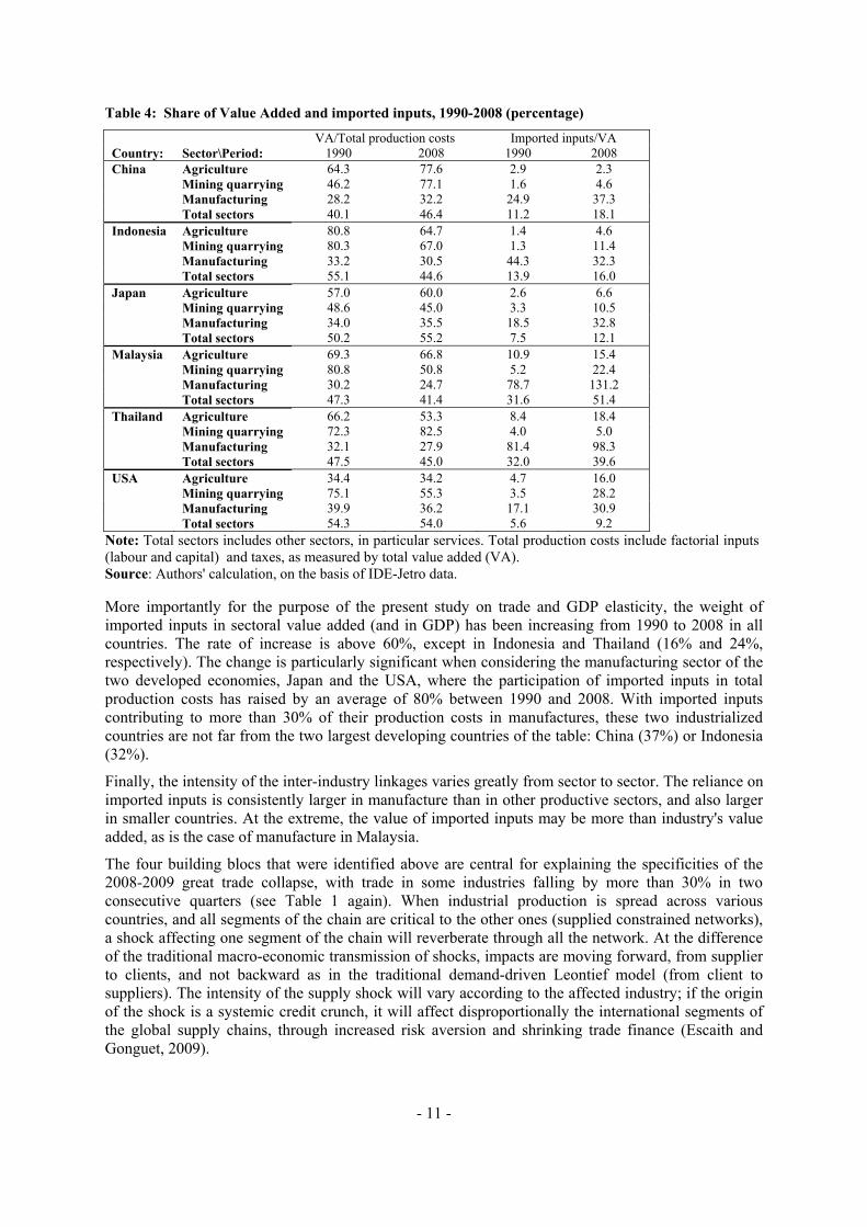
Table 4: Share of Value Added and imported inputs, 1990-2008 (percentage)

VA/Total production costs Imported inputs/VA Country: Sector\Period: 1990 2008 1990 2008 China Agriculture 64.3 77.6 2.9 2.3 Mining quarrying 46.2 77.1 1.6 4.6 Manufacturing 28.2 32.2 24.9 37.3 Total sectors 40.1 46.4 11.2 18.1 Indonesia Agriculture 80.8 64.7 1.4 4.6 Mining quarrying 80.3 67.0 1.3 11.4 Manufacturing 33.2 30.5 44.3 32.3 Total sectors 55.1 44.6 13.9 16.0 Japan Agriculture 57.0 60.0 2.6 6.6 Mining quarrying 48.6 45.0 3.3 10.5 Manufacturing 34.0 35.5 18.5 32.8 Total sectors 50.2 55.2 7.5 12.1 Malaysia Agriculture 69.3 66.8 10.9 15.4 Mining quarrying 80.8 50.8 5.2 22.4 Manufacturing 30.2 24.7 78.7 131.2 Total sectors 47.3 41.4 31.6 51.4 Thailand Agriculture 66.2 53.3 8.4 18.4 Mining quarrying 72.3 82.5 4.0 5.0 Manufacturing 32.1 27.9 81.4 98.3 Total sectors 47.5 45.0 32.0 39.6 USA Agriculture 34.4 34.2 4.7 16.0 Mining quarrying 75.1 55.3 3.5 28.2 Manufacturing 39.9 36.2 17.1 30.9 Total sectors 54.3 54.0 5.6 9.2

Note: Total sectors includes other sectors, in particular services. Total production costs include factorial inputs (labour and capital) and taxes, as measured by total value added (VA). Source: Authors' calculation, on the basis of IDE-Jetro data. More importantly for the purpose of the present study on trade and GDP elasticity, the weight of imported inputs in sectoral value added (and in GDP) has been increasing from 1990 to 2008 in all countries. The rate of increase is above 60%, except in Indonesia and Thailand (16% and 24%, respectively). The change is particularly significant when considering the manufacturing sector of the two developed economies, Japan and the USA, where the participation of imported inputs in total production costs has raised by an average of 80% between 1990 and 2008. With imported inputs contributing to more than 30% of their production costs in manufactures, these two industrialized countries are not far from the two largest developing countries of the table: China (37%) or Indonesia (32%).

Finally, the intensity of the inter-industry linkages varies greatly from sector to sector. The reliance on imported inputs is consistently larger in manufacture than in other productive sectors, and also larger in smaller countries. At the extreme, the value of imported inputs may be more than industry's value added, as is the case of manufacture in Malaysia.

The four building blocs that were identified above are central for explaining the specificities of the 2008-2009 great trade collapse, with trade in some industries falling by more than 30% in two consecutive quarters (see Table 1 again). When industrial production is spread across various countries, and all segments of the chain are critical to the other ones (supplied constrained networks), a shock affecting one segment of the chain will reverberate through all the network. At the difference of the traditional macro-economic transmission of shocks, impacts are moving forward, from supplier to clients, and not backward as in the traditional demand-driven Leontief model (from client to suppliers). The intensity of the supply shock will vary according to the affected industry; if the origin of the shock is a systemic credit crunch, it will affect disproportionally the international segments of the global supply chains, through increased risk aversion and shrinking trade finance (Escaith and Gonguet, 2009).

- 12 -

The following equations formalize these empirical observations from a demand-oriented input-output perspective.8 In absence of structural changes affecting production function (i.e., when technical coefficients, as described by an input-output matrix, are constant), the relationship linking demand for intermediate inputs with an external shock can be described by the following linear relationship:

ΔmIC = u' . M°. (I-A)-1 . ΔD Eq. 1

Where, in the case of a single country with "s" sectors: 9 ΔmIC : variation in total imported inputs (scalar) u': summation vector (1 x s) M°: diagonal matrix of intermediate import coefficients (s x s) (I-A)-1 : Leontief inverse, where A is the matrix of fixed technical coefficients (s x s) ΔD : initial shock on final demand (s x 1) 10

Similarly, changes in total production caused by the demand shock (including the intermediate inputs required to produce the final goods) is obtained from:

ΔQ = A . ΔQ + ΔD Eq. 2

Solving for ΔQ yields the traditional result:

ΔQ = (I-A)-1 . ΔD Eq. 3

Aggregating impacts across all sectors "s", the total additional output derived from this demand shock is equal to:

Δq = u' . ΔQ Eq. 4

The comparison between equations 1 and 4 is illustrative. Since [M°. (I-A)-1] is a linear combination of fixed coefficients, the ratio (ΔmIC / Δq) is a constant, and trade elasticity is 1. This results is consistent with the critics advanced by Bénassy-Quéré et al. (2009) against the hypothesis of the large trade multiplier observed during the crisis being attributed to supply chains and vertical integration.11

• Trade elasticity and the composition effect

The “steady-state approach” imbedded in structural input-output relationships tells only part of the story.12 We should remember that the initial shock ΔD is not a scalar, but a vector (s x 1). The individual shocks affecting each particular sector do not need to be always in the same proportion from one year to another one. We already saw on the Asian-USA case that the reliance on imported

8 Analysing the supply-shocks from the quantity space would pose a series of methodological issues

(Escaith and Gonguet, 2009). Notation uses macroeconomic practices and differs from usual IO conventions. 9 The model can be extended easily to the case of "n" countries by modifying accordingly the matrix A,

extending the IO relationship to include inter-sectoral international transactions of intermediate goods, and adapting the summation vector "u".

10 In this traditional IO framework considering one country and the rest of the world, exports of intermediate goods are considered as being part of the final demand. The situation differs when extending the IO relationship to include international transactions of intermediate consumptions, as in equation 1.

11 Using a slightly different approach, the authors conclude that “the growth rate of imports of domestic goods is the same as that of domestic GDP. ... When the trend of globalization is correctly accounted for, the income elasticity of imports is generally close to unity.” (page 15). Exploring the potential impact of the 2008-2009 downturn using a CGE model, using appropriate benchmarks for trade and GDP, the authors do not find any multiplier effect on trade.

12 “Steady-state” is used here in a loose sense of structurally stable dynamics; we are aware that the coexistence of such a Walrasian concept with the Keyenesian model of Leontief is particularly un-natural. Despite the conceptual contradiction, it is better suited to the CGE approach used by most contemporaneous trade analysts.

- 13 -

inputs is sector specific. As the sectoral import requirements [M°s] differ from sector to sector, then the apparent import elasticity for the national economy will change according to the sectoral distribution of the shock. 13

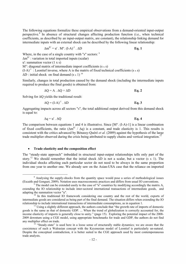
It was in particular the case after the financial crisis of September 2008, as demand for consumer durable and investment goods (consumer electronics, automobile and transport equipment, office equipment and computers, etc.) was particularly affected by the sudden stop in bank credits. Because these sectors are also vertically integrated, the impact on international trade in intermediate and final goods was high. Table 5 shows that the coefficient of imported inputs, derived from equation [1] are much larger than in other sectors, for example agriculture or services.

Table 5: Asia and USA: imported inputs coefficients, 2008.

Sector/ Country China Indonesia Japan Malaysia Thailand USA Agriculture 0.08 0.07 0.06 0.25 0.16 0.09 Mining quarrying 0.11 0.04 0.06 0.17 0.09 0.10 Manufacturing 0.24 0.25 0.14 0.71 0.50 0.17 Services 0.12 0.09 0.03 0.25 0.15 0.04 Total sectors 0.22 0.17 0.12 0.60 0.42 0.12 Note: Normalized imported inputs requirements (ΔmIC / Δd). Total sectors includes other sectors. Source: Authors' calculations on the basis of IDE-Jetro Asian Input-Output matrices.

Services sectors, which are the main contributors to GDP in developed countries and also the less dependent on imported inputs, were more resilient to the financial crisis than manufacture. But services and other non-tradable sector will eventually be affected by the external shock.

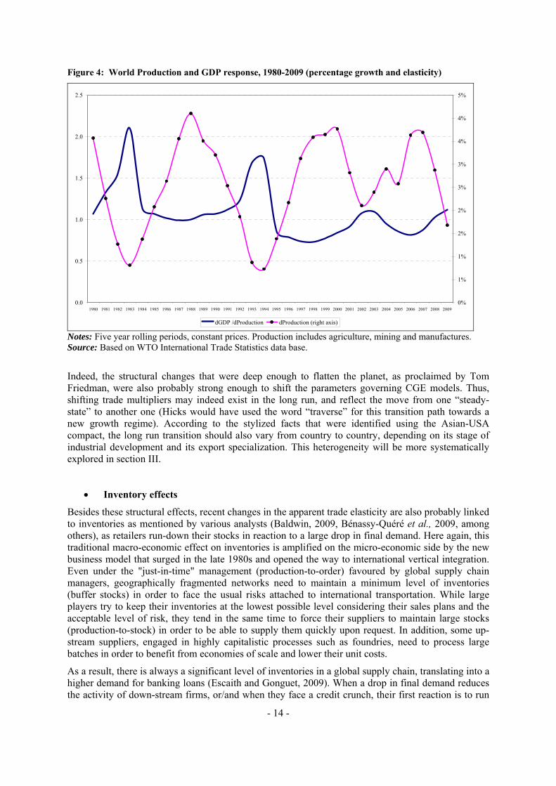
Because the initial shock was concentrated on manufacture and other tradable goods, the most vertically integrated sectors, the apparent Trade-GDP elasticity soared to approximately 5 (Figure 4). In a second phase, the initial shock reverberates through the rest of the economy, transforming the global financial crisis into a great recession. GDP continues to slow down but the decrease in trade tends to decelerate as the import content of services sectors (its sectoral imported input-VA ratio, as shown before in Table 4) is much lower than for manufacturing sectors.

After the initial overshooting of trade, it is therefore normal to expect a regression to normality of the trade elasticity for 2010. Or, to use the language of an econometrician, the data generation process should follow an error correction model (ECM). This hypothesis will be tested in Section IV. Nevertheless, as we also shall see in this essay (Section III) this does not mean that observed trade multipliers should be constant in the long run, as in the steady-case situation.

13 The more complex the production process, the more potential gains in outsourcing part of it; thus it is

natural to expect much more vertical integration in the manufacturing sector. Miroudot and Ragoussis (2009) show that manufacturing sectors in OECD countries generally use more imported inputs than other industrial and services sectors. It is specially the case for final consumer goods like ‘motor vehicles’ and ‘radio, TV and communication equipments’, or computers. Services are, as expected, less vertically integrated into the world economy. But even these activities show an upward trend in the use of imported services inputs (e.g. business services).

- 14 -

Figure 4: World Production and GDP response, 1980-2009 (percentage growth and elasticity)

0.0

0.5

1.0

1.5

2.0

2.5

1980 1981 1982 1983 1984 1985 1986 1987 1988 1989 1990 1991 1992 1993 1994 1995 1996 1997 1998 1999 2000 2001 2002 2003 2004 2005 2006 2007 2008 20090%

1%

1%

2%

2%

3%

3%

4%

4%

5%

dGDP /dProduction dProduction (right axis) Notes: Five year rolling periods, constant prices. Production includes agriculture, mining and manufactures. Source: Based on WTO International Trade Statistics data base.

Indeed, the structural changes that were deep enough to flatten the planet, as proclaimed by Tom Friedman, were also probably strong enough to shift the parameters governing CGE models. Thus, shifting trade multipliers may indeed exist in the long run, and reflect the move from one “steady-state” to another one (Hicks would have used the word “traverse” for this transition path towards a new growth regime). According to the stylized facts that were identified using the Asian-USA compact, the long run transition should also vary from country to country, depending on its stage of industrial development and its export specialization. This heterogeneity will be more systematically explored in section III.

• Inventory effects

Besides these structural effects, recent changes in the apparent trade elasticity are also probably linked to inventories as mentioned by various analysts (Baldwin, 2009, Bénassy-Quéré et al., 2009, among others), as retailers run-down their stocks in reaction to a large drop in final demand. Here again, this traditional macro-economic effect on inventories is amplified on the micro-economic side by the new business model that surged in the late 1980s and opened the way to international vertical integration. Even under the "just-in-time" management (production-to-order) favoured by global supply chain managers, geographically fragmented networks need to maintain a minimum level of inventories (buffer stocks) in order to face the usual risks attached to international transportation. While large players try to keep their inventories at the lowest possible level considering their sales plans and the acceptable level of risk, they tend in the same time to force their suppliers to maintain large stocks (production-to-stock) in order to be able to supply them quickly upon request. In addition, some up-stream suppliers, engaged in highly capitalistic processes such as foundries, need to process large batches in order to benefit from economies of scale and lower their unit costs.

As a result, there is always a significant level of inventories in a global supply chain, translating into a higher demand for banking loans (Escaith and Gonguet, 2009). When a drop in final demand reduces the activity of down-stream firms, or/and when they face a credit crunch, their first reaction is to run

- 15 -

down their inventories. Thus, a slow-down in activity transforms itself into a complete stand-still for the supplying firms that are located up-stream.

These amplified fluctuations in ordering and inventory levels result in what is known as "bullwhip effect" in the management of production-distribution systems (Stadtler, 2008). This effect is more sensitive in an international setting. Alessandria et al. (2009) provide direct evidence that participants in international trade face more severe inventory management problems. Importing firms have inventory ratios that are roughly twice those of firms that only purchase materials domestically, and the typical international order tends to be about 50 percent larger and half as frequent as the typical domestic one. The related international trade flows, at the micro-economic level, are therefore lumpy and infrequent. As long as the down-stream inventories of imported goods have not been reduced to their new optimum level, foreign suppliers are facing a sudden stop in their activity and must reduce their labour force or keep them idle.

The timing and intensity of the international transmission of supply shocks may differ from traditional demand shocks applying on final goods. For example, the supply-side transmission index proposed by Escaith and Gonguet (2009) implicitly assumes that all secondary effects captured by the IO matrix occur simultaneously, while these effects may actually propagate more or less quickly depending on the length of the production chain. Also, there might be contractual pre-commitments for the order of parts and material that manufacturers have to place well in advance in order to secure just-in-time delivery in accordance to their production plans (Uchida and Inomata, 2009).

Nevertheless, in closely integrated networks, these mitigating effects are probably reduced, especially when the initial shock is large. A sudden stop in final demand is expected to reverberate quickly thorough the supply chain, as firms run-down their inventories in order to adjust to persistent changes in their market. This inventory effect magnifies demand shocks and is principally to blame for the initial collapse of trade in manufacture that characterized the world economy from September 2008 to June 2009. A study on the electronic equipment sector during the crisis (Dvorak, 2009) indicates that a fall in consumer purchase of 8% reverberated into a 10% drop in shipments of the final good and a 20% reduction in shipments of the related intermediate inputs (e.g., computer chips and other parts). The velocity of the cuts was much faster than in previous slumps, as reordering is now done on a weekly basis, instead of the monthly or quarterly schedules that prevailed up to the early 2000s.

III. GLOBAL, SECTORAL AND REGIONAL TRADE ELASTICITY PATTERNS

The preceding sections provided information on the diversity of country/sectoral situation in an epitome (the USA-Asian compact), using accounting relationships. In this section, we extend the data analysis to the rest of the world, in order to identify patterns illustrative of the GDP elasticity of imports and the putative role of supply chains. We start by extracting stylized facts at world level using a set of standard regressions, then analyzing how the parameters of interest vary according to specific groupings of observations, or change with time. It should be noted that the results presented in this section are exploratory, and do not pretend to provide a strong statistical basis for confirmatory inferences or predictions. For this purpose, more formal dynamic specifications will be presented in the last section of this paper.

The data supporting the exploration are obtained from the IMF's World Economic Outlook 2009. World GDP weighted at market exchange rates 14 is constructed by combining World GDP at 2000 prices from the WDI database (World Bank) with GDP growth rates (market exchange rate) from the WEO2009 (IMF). Our sample comprises annual data between 1980 and 2009.

14 World GDP is usually weighted with PPP, which, however, is inadequate when investigating demand on international markets (i.e. GDP-trade elasticity).

- 16 -

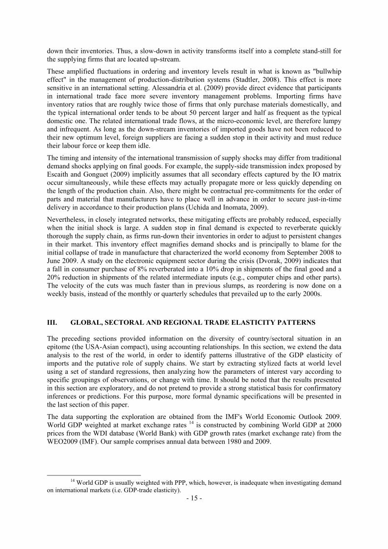
• Global patterns The GDP elasticity of imports aggregated at world level is estimated in a first step by OLS:

ttt ym εβα ++= Eq. 5

with tm = logarithmized imports, ty = logarithmized GDP and tε = residuals.

We obtain an elasticity of 2.28 for the full sample (R²= 0.99 for 30 observations).

As a robustness check and to provide a benchmark for subsequent calculations, we estimate a state space object containing GDP and imports, to which we apply a Kalman Filter, with maximum likelihood:

Signal: ttttt ym εβα ++= Eq. 6 State: ttt νββ += −1 Eq. 7

The estimated elasticity is also 2.28.

To explore and validate the likelihood of the hypothesis of global supply chains having led to an increase of the GDP elasticity of imports — transition from one steady state (without global supply chains) to another one (with global supply chains — we should observe changing elasticities patterns over time and across the sample.

To visualize the changing characteristics over time, we redo the estimations both with OLS and Kalman Filter for rolling time windows of each 10 years, i.e. the estimation sample subsequently changes by one year, the first sample comprising 1980 – 1989, the second 1981 – 1990 and so forth. Results are displayed graphically in Figure 5.

Each data point of the graph reflects the estimated coefficient for the previous 10 years, e.g. the displayed value in the year 2000 reflects the GDP elasticity of imports computed for the 10-year window between 1991 and 2000. Both graphs show clearly, that the GDP elasticity of imports is not at all constant and changes over the years.

The graphs feature quite closely the trend that should be expected if the hypothesis of the impact of global supply chains on trade elasticities and a traverse from one steady state to another one were correct. From 1989 to 1998, we can observe a steady increase in the elasticity from about 1.6 to 3.0, which in the following six years decreases again.

Figure 5 GDP Elasticity of Imports – World (constant prices)

1.6

2.0

2.4

2.8

3.2

90 92 94 96 98 00 02 04 06 08

GDP Elasticity of ImportsOLS Estimation

Rolling Windows of 10 years

World

1.6

2.0

2.4

2.8

3.2

90 92 94 96 98 00 02 04 06 08

GDP Elasticity of ImportsKalman filter


World

Source: Author’s calculations. Data description see text.

- 17 -

Between 2004 and 2008 a stabilization at a level of about 2.3 has taken place, before a predicted decrease in the crisis year 2009. Thus, the observed data patterns seem to strengthen the hypothesis that trade elasticity has increased in the years of rising globalization in the 1990s and turned back to a new steady state that has been reached around 2004.

But even if these results seem to support the hypothesis of a structural change in world trade – compatible with the role of supply chains in explaining the increased elasticity of imports to GDP – it should be pointed out that the conducted analysis does not give any information on the causes of the observed change. Therefore, we continue the explorative data analysis by looking at sub-groups of countries. If the global supply chains were the cause for the observed change in elasticities, the results should be similar for countries participating heavily in global supply chains and a different trend should be observed in the rest of countries.

• Exploring country patterns

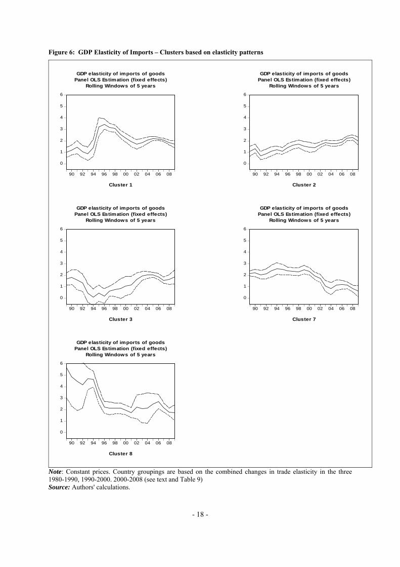
The objective of the section is to explore in more details the data generation process and identify possible clusters of countries. We conduct the following analysis with the group of the 50 most important exporters15 as listed in WTO (2008b, p.12 Table I.8). For the analysis, we use data from the IMF's World Economic Outlook 200916, namely imports of goods (volume) and gross domestic product (in constant prices) in a sample from 1980 to 2009. In order to address the trade-off between number of observations and disaggregation, we take advantage of the panel dimension of our data and cluster the countries in an appropriate way.17

As a first approach to defining groups among countries, we cluster them according to observed data patterns. For this purpose, we estimate the elasticity of imports to GDP using a state space object for each individual country and apply a Kalman Filter for three different samples: 1980-1990, 1990-2000, and 2000-2008. The results provide a first idea of how the elasticity of imports is evolving for each country in the sample. Then, we construct up to 9 different clusters (3 x 3) 18 with the following logic:

- Does the elasticity from sample one to sample three increase, remain stable or decrease (3 options)? - If so, does the elasticity of the second sample lay above, in between or beneath the two other elasticities (another 3 possible cases)?

15 Chinese Taipei is excluded due to data availability. Thus, we analyze the remaining 49 countries of

the group of the 50 leading exporters in world merchandise trade in 2007, namely Algeria, Argentina, Australia, Austria, Belgium, Brazil, Canada, Chile, China, Czech Republic, Denmark, Finland, France, Germany, Hong Kong, China, Hungary, India, Indonesia, Iran, Ireland, Israel, Italy, Japan, Korea, Kuwait, Malaysia, Mexico, Netherlands, Nigeria, Norway, Philippines, Poland, Portugal, Russian Federation, Saudi Arabia, Singapore, Slovak Republic, South Africa, Spain, Sweden, Switzerland, Thailand, Turkey, Ukraine, United Arab Emirates, United Kingdom, United States, Venezuela, and Viet Nam.

16 From 1980 - 1991 data for GDP and imports for Russia and the Ukraine are missing in WEO2009. These missing values are replaced with the corresponding values from WEO2008. As all GDP values of Russia in WEO2009 were multiplied with 1.1362 (in comparison to the WEO2008) the added values were also multiplied with the same factor.

17 It is important to point out that contrary to the world aggregate, where countries are weighted by their GDP; all countries have the same weight in the following clusters. Thus, comparison with the results of Figure 5 is somehow biased.

18 Actual number of cluster (see Tables 8 and 9 in Annex) is smaller as no country pertains to clusters 4, 5 or 6, which have in common that the elasticity from sample one to sample three remains stable. Cluster 9 (decrease, with the second elasticity beneath the first and the third elasticity) is omitted, as only one country falls in this category.

- 18 -

Figure 6: GDP Elasticity of Imports – Clusters based on elasticity patterns

0

1

2

3

4

5

6

90 92 94 96 98 00 02 04 06 08

GDP elasticity of imports of goodsPanel OLS Estimation (fixed effects)


Cluster 1

0

1

2

3

4

5

6

90 92 94 96 98 00 02 04 06 08



Cluster 2

0

1

2

3

4

5

6

90 92 94 96 98 00 02 04 06 08



Cluster 3

0

1

2

3

4

5

6

90 92 94 96 98 00 02 04 06 08



Cluster 7

0

1

2

3

4

5

6

90 92 94 96 98 00 02 04 06 08



Cluster 8

Note: Constant prices. Country groupings are based on the combined changes in trade elasticity in the three 1980-1990, 1990-2000. 2000-2008 (see text and Table 9) Source: Authors' calculations.

- 19 -

We arrive at the following country groups (see Table 9 in the appendix). Cluster 1: countries with an increasing elasticity over the full sample, which overshoots in the middle of the sample; cluster 2: countries with an increasing elasticity over the full sample; cluster 3: countries with an increasing elasticity over the full sample, but with a drop in the middle of the sample; cluster 7: countries with a decreasing elasticity over the full sample, but with an increase in the middle of the sample; and cluster 8: countries with a decreasing elasticity over the full sample. The results of the panel OLS estimation with fixed cross-section effects and rolling windows of 5 years are displayed in Figure 6.

As the data show, only the first cluster of countries features a trend compatible with our hypothesis of global supply chains being the cause for the change in elasticities. If this cluster contained all the countries that participate in global supply chains, the before mentioned hypothesis would be enormously strengthened. Table 9 in the appendix shows that many of the participants of global supply chains are actually in the cluster. However, many others which are known for their participation in global supply chains, like Germany, China or Mexico, are missing, which suggest that it might be just coincidence that some of the countries show the data structure that confirms the above mentioned hypothesis.

Overall, given these findings, we rather tend not to accept the hypothesis that global supply chains explain all by themselves the changes in trade-income elasticity. However, this does not imply that the emergence of global production networks since the late 1980s did not play a role, only that other factors may also be at work to explain the results observed when estimating equations 5 to 7.

• Clustering by export specialization

As the clustering by pure elasticity patterns cannot confirm the hypothesis of global supply chains being the driving force behind the change in the GDP elasticity of imports, we cluster the countries in an alternative way, based on some economic rational. We will group all those countries together, that have the same export specialization. Main export activities are given by UNCTAD in its table "Country trade structure by product group" (UNCTAD, 2008, Table 3.1). Thus, we obtain the following five clusters (details are given in Table 9 in the appendix): fuel exporters; ores, metals, precious stones and non-monetary gold exporters; manufactured goods exporters; machinery and transport equipment exporters; and other manufactured goods exporters.19 Results of panel OLS estimations with fixed cross-section effects and rolling windows of 5 years are displayed graphically in Figure 7..

Again, the patterns of the calculated elasticities change significantly among the different clusters of countries. The elasticity of the group of fuel exporters increases steadily, which however is certainly a terms-of-trade effect and has nothing to do with the globalization of supply chains. For the manufacturing sector, both for the aggregate (manufacturing exporters) and for the two subgroups (machinery exporters and other manufactured goods exporters) there have been three peaks in trade elasticity, the first one in 1990, the second in 1998, and the third in 2005.

Each time, elasticity has decreased in between. This however, does not support the hypothesis of an impact of supply chains on the elasticity either. Thus, we still do not find supporting evidence for the implication of the globalized supply chains in the changes of trade elasticities.20

19 The following three product groups were not considered in the analysis, as they comprise less than three countries: all food items; agricultural raw materials; chemical products.

20 Yet another way of clustering the countries by export specialization, using the main export products of each country, does not change the result qualitatively either: the hypothesis of an impact of the global supply chains on the changes in GDP elasticity of imports can still not be confirmed by our explorative data analysis. The results of this robustness check can be found in the appendix in Figure 10 and Figure 11.

- 20 -

Figure 7: GDP Elasticity of Imports – Cluster based on export specialization

Note: Constant prices. See text and Tables 8 and 9 for methodology and groupings Source: Authors' calculations.

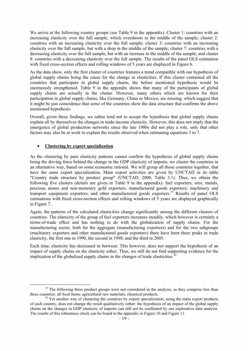
• Clustering by regions To complete the exploration of trade elasticity patterns, we cluster the countries by (geographical) regions. Within one regional cluster the countries often dispose of a similar endowment and may, accordingly, have assumed a similar role in the world economy. For example, the literature often

0

1

2

3

90 92 94 96 98 00 02 04 06 08



Cluster Fuels Exporters

0

1

2

3

90 92 94 96 98 00 02 04 06 08



Cluster Mining Exporters

0

1

2

3

90 92 94 96 98 00 02 04 06 08



Cluster Manufacturing Exporters

0

1

2

3

90 92 94 96 98 00 02 04 06 08



Cluster Machinery Exporters

0

1

2

3

90 92 94 96 98 00 02 04 06 08



Cluster Other Manufactured Products Exporters

- 21 -

Figure 8: GDP Elasticity of Imports - Regions

Note: Constant prices. See text and Table 9 for methodology and groupings. Source: Authors' calculations.

0

1

2

3

4

90 92 94 96 98 00 02 04 06 08



Cluster Western European Countries

0

1

2

3

4

90 92 94 96 98 00 02 04 06 08



Cluster G7 Countries

0

1

2

3

4

90 92 94 96 98 00 02 04 06 08



Cluster Emerging Asia

0

1

2

3

4

90 92 94 96 98 00 02 04 06 08



Cluster New EU Members

0

1

2

3

4

90 92 94 96 98 00 02 04 06 08



Cluster Latin America

0

1

2

3

4

90 92 94 96 98 00 02 04 06 08



Cluster Middle East

- 22 -

refers to Central and Eastern European Countries (CEEC) or Emerging Asia as one entity when discussing offshoring. Therefore, we construct the following set of clusters: Latin America, Emerging Asia, New EU-Member States, Middle East, G7-Countries, and Western European Countries (see Table 9 in the appendix). Results of the panel OLS estimation with fixed cross-section effects for rolling windows of five years of the GDP elasticity of imports are displayed graphically in Figure 8.

As can be observed, elasticities vary substantially between the different regions but, overall, there is no evidence for a strengthening of the supply-chain hypothesis. The evolution of the elasticity of the New EU-Member countries could be an illustration of a transition that has taken place, but at the same time the graph for the countries of the Middle East clearly allude to the limitations of the trade elasticity approach: the exploration of the data patterns does not say anything about the causes of the change in elasticity. In the case of the latter group of countries, the increase in elasticity most probably is due to changes in relative prices and is not related at all to the globalization of supply chains.

To sum up, even ignoring the known limitations of the model, we cannot find strong evidence for the role of global supply chains for the changes in the GDP elasticity of imports. Although on the aggregated world level trade elasticity is changing in a way that one could be tempted to interpret like confirming evidence (trade elasticity increased in the years of rising globalization in the 1990s, then fall back to lower level in the mid-2000s), the disaggregated analysis does not support this hypothesis. Some countries that are part of global supply chains do not show significant differences in the evolution of their elasticities, while countries less integrated in global production networks tend to do so. Trade elasticities are in general quite volatile, but the exploration of elasticity patterns does not support the hypothesis that deeper vertical integration is "the" driving force behind this development. There are probably more causal factors at work. We mentioned the changes in relative prices which inflated the value of primary commodities. Other factors among others could include the lowering of trade barriers after the conclusion of the Uruguay Round in 1995, or the increasing taste of consumers for diversity as their income increased.

IV. AN ESTIMATION WITH THE ERROR CORRECTION MODEL

The previous sections were exploratory and no formal assumption was made on the kind of relationship existing between imports and GDP. We now assume that there is a long-run equilibrium relationship between the growth of trade and the growth of GDP, i.e. the elasticity is stable in the long-run. As described in the introduction and evidenced in the above mentioned Figure 5, we expect the elasticity of trade to GDP to have increased during the 1990s because of outsourcing and offshoring but to have decreased afterwards, once a new steady state had been reached. The elasticity that we measure through trade and GDP data is a short-run elasticity that reflects both the long-run equilibrium and the stochastic fluctuations leading to volatility, such as those illustrated in section II (sequential nature of sectoral shocks, inventory effects, etc.).

We use an Error Correction Model (ECM) to account for this and to estimate the steady-state elasticity. We work with quarterly data from the OECD National Accounts database over the period 1961-200921 in order to have a consistent dataset with time-series for the OECD area (based on 24 OECD economies) and individual data for 30 OECD countries. The data, in constant prices, allow to control for the changes in relative price, one of the source of fluctuations identified in the previous sections.

21 Year-on-year change, volumes in USD (fixed PPPs, OECD reference year), seasonally adjusted.

Market exchange rates are used for the OECD aggregation.

- 23 -

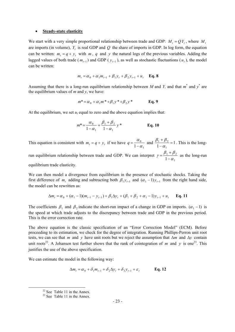
• Steady-state elasticity We start with a very simple proportional relationship between trade and GDP: tt YQM = , where tM are imports (in volume), tY is real GDP and Q the share of imports in GDP. In log form, the equation can be written: tt yqm += with m , q and y the natural logs of the previous variables. Adding the lagged values of both trade ( 1−tm ) and GDP ( 1−ty ), as well as stochastic fluctuations ( tu ), the model can be written:

ttttt uyymm ++++= −− 121110 ββαα Eq. 8

Assuming that there is a long-run equilibrium relationship between M and Y, and that m* and y* are the equilibrium values of m and y, we have:

**** 2110 yymm ββαα +++= Eq. 9

At the equilibrium, we set ut equal to zero and the above equation implies that:

*11

*1

21

1

0 ymαββ

αα

−+

+−

= Eq. 10

This equation is consistent with tt yqm += if we have 1

0

1 αα−

=q and 11 1

21 =−+αββ

. This is the long-

run equilibrium relationship between trade and GDP. We can interpret 1

21

1 αββ

γ−+

= as the long-run

equilibrium trade elasticity.

We can then model a divergence from equilibrium in the presence of stochastic shocks. Taking the first difference of tm adding and subtracting both 11 −tyβ and 11 )1( −− tyα from the right hand side, the model can be rewritten as:

tttttt uyyymm +−+++Δ+−−+=Δ −−− 112111110 )1())(1( αβββαα Eq. 11

The coefficients 1β and 2β indicate the short-run impact of a change in GDP on imports. )1( 1 −α is the speed at which trade adjusts to the discrepancy between trade and GDP in the previous period. This is the error correction rate.

The above equation is the classic specification of an “Error Correction Model” (ECM). Before proceeding to its estimation, we check for the degree of integration. Running Phillips-Perron unit root tests, we can see that m and y have unit roots but we reject the assumption that mΔ and yΔ contain unit roots22. A Johansen test further shows that the rank of cointegration of m and y is one23. This justifies the use of the above specification.

We can estimate the model in the following way:

ttttt yymm εδδδα ++Δ++=Δ −− 132110 Eq. 12

22 See Table 11 in the Annex. 23 See Table 11 in the Annex.

- 24 -

The latter equation is similar to the former one with 1211 ,1 βδαδ =−= and 213 ββδ += . The advantage of the specification is that we can derive directly the long-run equilibrium trade elasticity

from the estimated coefficients: 1

3

1

21

1 δδ

αββ

γ =−

+= . Furthermore, 1δ is the speed at which imports

adjust to trade and 2δ is the short-term impact of GDP on trade (short-term elasticity).

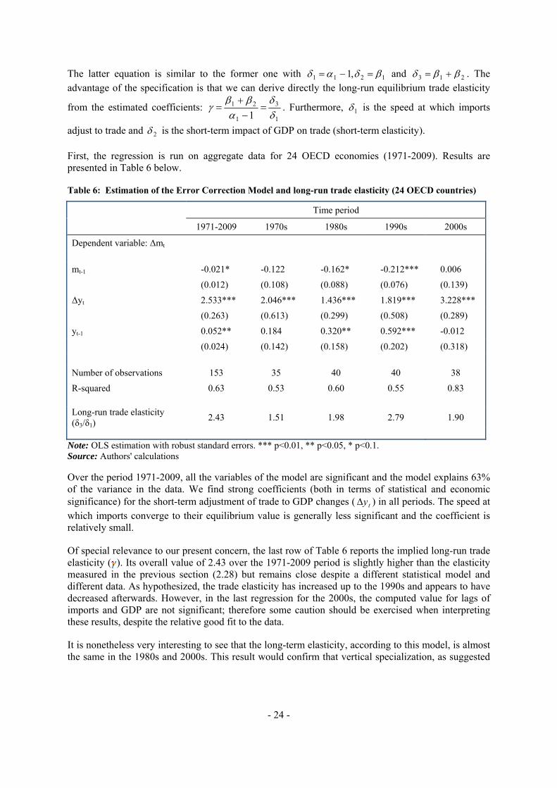
First, the regression is run on aggregate data for 24 OECD economies (1971-2009). Results are presented in Table 6 below.

Table 6: Estimation of the Error Correction Model and long-run trade elasticity (24 OECD countries)

Time period

1971-2009 1970s 1980s 1990s 2000s

Dependent variable: Δmt mt-1 -0.021* -0.122 -0.162* -0.212*** 0.006

(0.012) (0.108) (0.088) (0.076) (0.139)

Δyt 2.533*** 2.046*** 1.436*** 1.819*** 3.228***

(0.263) (0.613) (0.299) (0.508) (0.289)

yt-1 0.052** 0.184 0.320** 0.592*** -0.012

(0.024) (0.142) (0.158) (0.202) (0.318) Number of observations 153 35 40 40 38

R-squared 0.63 0.53 0.60 0.55 0.83 Long-run trade elasticity (δ3/δ1)

2.43 1.51 1.98 2.79 1.90

Note: OLS estimation with robust standard errors. *** p<0.01, ** p<0.05, * p<0.1. Source: Authors' calculations Over the period 1971-2009, all the variables of the model are significant and the model explains 63% of the variance in the data. We find strong coefficients (both in terms of statistical and economic significance) for the short-term adjustment of trade to GDP changes ( tyΔ ) in all periods. The speed at which imports converge to their equilibrium value is generally less significant and the coefficient is relatively small.

Of special relevance to our present concern, the last row of Table 6 reports the implied long-run trade elasticity ( ). Its overall value of 2.43 over the 1971-2009 period is slightly higher than the elasticity measured in the previous section (2.28) but remains close despite a different statistical model and different data. As hypothesized, the trade elasticity has increased up to the 1990s and appears to have decreased afterwards. However, in the last regression for the 2000s, the computed value for lags of imports and GDP are not significant; therefore some caution should be exercised when interpreting these results, despite the relative good fit to the data.

It is nonetheless very interesting to see that the long-term elasticity, according to this model, is almost the same in the 1980s and 2000s. This result would confirm that vertical specialization, as suggested

- 25 -

by theory, has no reason to increase the equilibrium elasticity of trade to GDP and that the 1990s, with their higher trade elasticity, can be interpreted as a transition period to a new "steady-state". 24

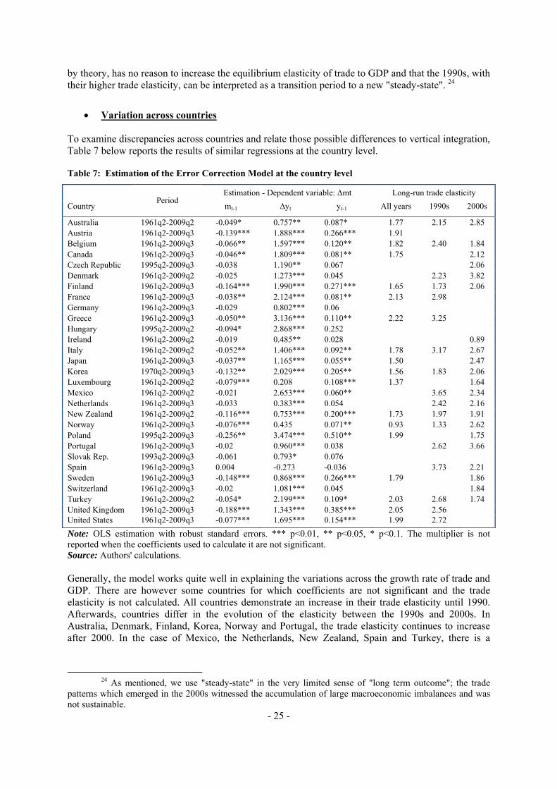
• Variation across countries

To examine discrepancies across countries and relate those possible differences to vertical integration, Table 7 below reports the results of similar regressions at the country level.

Table 7: Estimation of the Error Correction Model at the country level

Estimation - Dependent variable: Δmt Long-run trade elasticity Country

Period mt-1 Δyt yt-1 All years 1990s 2000s

Australia 1961q2-2009q2 -0.049* 0.757** 0.087* 1.77 2.15 2.85 Austria 1961q2-2009q3 -0.139*** 1.888*** 0.266*** 1.91 Belgium 1961q2-2009q3 -0.066** 1.597*** 0.120** 1.82 2.40 1.84 Canada 1961q2-2009q3 -0.046** 1.809*** 0.081** 1.75 2.12 Czech Republic 1995q2-2009q3 -0.038 1.190** 0.067 2.06 Denmark 1961q2-2009q2 -0.025 1.273*** 0.045 2.23 3.82 Finland 1961q2-2009q3 -0.164*** 1.990*** 0.271*** 1.65 1.73 2.06 France 1961q2-2009q3 -0.038** 2.124*** 0.081** 2.13 2.98 Germany 1961q2-2009q3 -0.029 0.802*** 0.06 Greece 1961q2-2009q3 -0.050** 3.136*** 0.110** 2.22 3.25 Hungary 1995q2-2009q2 -0.094* 2.868*** 0.252 Ireland 1961q2-2009q2 -0.019 0.485** 0.028 0.89 Italy 1961q2-2009q2 -0.052** 1.406*** 0.092** 1.78 3.17 2.67 Japan 1961q2-2009q3 -0.037** 1.165*** 0.055** 1.50 2.47 Korea 1970q2-2009q3 -0.132** 2.029*** 0.205** 1.56 1.83 2.06 Luxembourg 1961q2-2009q2 -0.079*** 0.208 0.108*** 1.37 1.64 Mexico 1961q2-2009q2 -0.021 2.653*** 0.060** 3.65 2.34 Netherlands 1961q2-2009q3 -0.033 0.383*** 0.054 2.42 2.16 New Zealand 1961q2-2009q2 -0.116*** 0.753*** 0.200*** 1.73 1.97 1.91 Norway 1961q2-2009q3 -0.076*** 0.435 0.071** 0.93 1.33 2.62 Poland 1995q2-2009q3 -0.256** 3.474*** 0.510** 1.99 1.75 Portugal 1961q2-2009q3 -0.02 0.960*** 0.038 2.62 3.66 Slovak Rep. 1993q2-2009q3 -0.061 0.793* 0.076 Spain 1961q2-2009q3 0.004 -0.273 -0.036 3.73 2.21 Sweden 1961q2-2009q3 -0.148*** 0.868*** 0.266*** 1.79 1.86 Switzerland 1961q2-2009q3 -0.02 1.081*** 0.045 1.84 Turkey 1961q2-2009q2 -0.054* 2.199*** 0.109* 2.03 2.68 1.74 United Kingdom 1961q2-2009q3 -0.188*** 1.343*** 0.385*** 2.05 2.56 United States 1961q2-2009q3 -0.077*** 1.695*** 0.154*** 1.99 2.72

Note: OLS estimation with robust standard errors. *** p<0.01, ** p<0.05, * p<0.1. The multiplier is not reported when the coefficients used to calculate it are not significant. Source: Authors' calculations. Generally, the model works quite well in explaining the variations across the growth rate of trade and GDP. There are however some countries for which coefficients are not significant and the trade elasticity is not calculated. All countries demonstrate an increase in their trade elasticity until 1990. Afterwards, countries differ in the evolution of the elasticity between the 1990s and 2000s. In Australia, Denmark, Finland, Korea, Norway and Portugal, the trade elasticity continues to increase after 2000. In the case of Mexico, the Netherlands, New Zealand, Spain and Turkey, there is a

24 As mentioned, we use "steady-state" in the very limited sense of "long term outcome"; the trade

patterns which emerged in the 2000s witnessed the accumulation of large macroeconomic imbalances and was not sustainable.

- 26 -

decrease in the elasticity as seen with the aggregate data in Table 6. For other countries, the results are not significant enough to assess the trend.

• Trade response to external shocks

On Figure 9 is represented the "Impulse Response Function" (IRF) of imports when there is an exogenous shock on GDP (calculated on the basis of the estimation of the OECD time-series for 1999-2009). When there is a 1% decrease in GDP, we can see that during the first year following the shock trade decreases more than proportionally and “over-reacts” (there is a 3% decrease in imports). Then, there is a convergence towards a new equilibrium value. Trade recovers during the second and third years; 4 years after the shock the decrease in trade is about 2%, in line with the multiplier observed in Table 6 (1.9).

Figure 9: Impulse Response Function (IRF) Impact of an exogenous decrease in GDP on trade (24 OECD countries)

-.04

-.03

-.02

-.01

0

1 2 3 4

Years

Note: Orthogonalized IRF based on the estimation of the OECD model for the period 1999-2009.

• Role of vertical specialization

In order to check more precisely for the influence of international supply chains in the change in trade elasticity, we change the model and introduce a vertical specialization variable. 25

25 Cheung and Guichard (2009) suggest that the way vertical specialisation affects trade is by raising its

elasticity with respect to income.

- 27 -

The estimated equation becomes:

tttttt VSyVSyymm εδδδδδα ++++Δ++=Δ −−− 514132110 * Eq. 13

where VS is the country vertical specialization share, calculated as in Hummels et al. (2001)26. VS is closely related to the imported content of intermediate goods derived previously from equation [1] in an input-output context.

The vertical specialization variables slightly increase the goodness-of-fit of the model for most countries but are not always significant. To see to what extent vertical specialization can help to explain the trade collapse during the crisis, we do a forecasting exercise. For each quarter, we predict the value of imports based on the estimated model. We then compare the results between the first model (without vertical specialization) and the second model (with vertical specialization). As it can be seen in Table 12 in the Annex, the discrepancy between the predicted change in trade and the observed trade collapse is only marginally reduced when using the specification with vertical specialization. The difference in percentage points tends to be lower for most countries but not in a way that has significantly increased the ability of the model to predict the trade collapse, even if vertical specialization has shaped the dynamics of transmission. V. CONCLUSION

The paper investigates the role of global supply chains in explaining the trade collapse of 2008-2009, in line with the long-term rise observed in trade elasticity since the 1980s. After reviewing the literature, the study adopts an empirical strategy based on two complementary steps. Stylized facts are first derived from (i) the observation of interrelated input-output matrices for a demonstrative sub-set of countries (Asia and the USA), and (ii) from the use of exploratory analysis on a large and diversified sample of countries, of different income and development levels, regions and resource endowments. The results obtained from this exploratory phase highlight that import elasticities have been in general very volatile and suggest the specification of a statistical ECM model to measure the respective short-term and long-term dynamics of trade elasticity. An ECM model is therefore used in a third phase, to formally probe the role of vertical integration in explaining changes in trade elasticity. Aggregated results obtained using both exploratory and ECM models tend to support the hypothesis that long-term trade elasticity has raised during the 1990s, before lowering in the late 2000s. The concept of steady state equilibrium implies, however, that vertical integration should only affect the level of trade relative to GDP but not the elasticity. While we expect the trade elasticity to be stable in the long-run, we also recognize that the pattern observed from the data is compatible with a structural change from one steady state (a "Ricardian" economy where countries trade final goods) to another one (a "trade in tasks" economy, where countries trade also intermediate goods in a global supply chain). Accordingly, from the late 1980s onwards, the internationalization of production has caused a shift from one steady state to a new one with trade elasticities rising only during the transition phase, coming back then to their long-run equilibrium level, at a new steady state where trade represents a higher share of GDP.

26 Data come from Miroudot and Ragoussis (2009). Time-series have been created over the period

1995-2009 with 3 data points (1995, 2000 and 2005 for most countries). Because data are interpolated and extrapolated, there is no guarantee that the variable accurately reflects the variation over time of the vertical specialisation share. The assumption is that this share is relatively stable over years and that the trend suggested by the three data points is enough to account for its evolution.

- 28 -

In the short run, the paper shows that a shock affecting differently distinctive sectors of the economy could also have an transitory impact on the trade elasticity of the whole economy, explaining some of the volatility observed in the data. Moreover, two supply-chain related factors are at work to explain the overshooting of trade elasticity that occurred during the 2008-2009 trade collapse. The first one is the composition effect, as the initial demand shocks linked to the credit crunch concentrated disproportionably on consumer durables and investment goods, the most vertically integrated industrial sectors; the second one is the "bullwhip effect" where inventory adjustments are amplified as one moves upstream in the supply chain. But the disturbance is expected to dissipate and the elasticity to return to its long-run value. As our ECM results show, this pattern can be observed for the import multiplier calculated for the world aggregate. On the other hand, while the aggregate results did provide ground for the shifting-steady state hypothesis, disaggregated analysis could not confirm the generality of the hypothesis. Indeed, a more detailed analysis showed significant differences among trade elasticities for different countries and sectors. The direct observation of intra-sectoral trade, using input-output models, as well as standard time-series econometrics tends to identify the aggregate pattern in many countries, including Japan and the USA. However, others which are also known for their participation in global supply chains, like Germany, China or Mexico, are not showing the expected long-term increase in trade elasticity, suggesting that it might be just coincidence that some of the countries show the data structure that confirms the above mentioned hypothesis. Moreover, when a more formal specification is used, and vertical specialization is explicitly included as an explanatory variable, the results are again inconclusive. Overall, given these findings, we rather tend not to accept the hypothesis that global supply chains explain all by themselves the changes in trade-income elasticity. However, this does not imply that the emergence of global production networks since the late 1980s did not play a role — our results clearly indicate that they did have a role — but only that other factors may also be at work to explain the diversity of the observed results.

*************

- 29 -

REFERENCES Agnese, P. and Ricart, J. E. (2009) “Offshoring: Facts and Numbers at the Country Level”.

Working paper, IESE Business School - Universidad de Navarra. Alessandria, G., J. Kaboski and V. Midrigan (2009) "Inventories, Lumpy Trade, and Large

Devaluations" American Economic Review, forthcoming. Antràs, P. and Helpman, E. (2004) “Global Sourcing”. Journal of Political Economy, 112(3), 552–

580. Baldwin, R. (ed.) (2009) "The great trade collapse: Causes, Consequences and Prospects" VoxEU.org Baldwin, R. (2006) "Globalisation: the great unbundling(s)" Economic Council of Finland,

20 September. Bénassy-Quéré, A., Decreux, Y., Fontagné, L. and Khoudour-Casteras D. (2009) “Economic

Crisis and Global Supply Chains”. Document de Travail 2009-15, Centre d’Etudes Prospectives et d’Informations Internationales (CEPII).

Bergin, P. R., Feenstra, R. C. and Hanson, G. H. (2009) “Offshoring and Volatility: Evidence from Mexico’s Maquiladora Industry”. American Economic Review, 99(4), 1664–1671.

Borchert, I. and Mattoo, A. (2009) “The crisis-resilience of services trade”. Policy Research Working Paper Series 4917, The World Bank.

Chen, Y., Ishikawa, J. and Yu, Z. (2004) “Trade liberalization and strategic outsourcing”. Journal of International Economics, 63(2), 419–436.

Cheung, C. and Guichard, S. (2009) “Understanding the World Trade Collapse”. OECD Economics Department Working Papers 729, OECD, Economics Department.

Coucke, K. and Sleuwaegen, L. (2008) “Offshoring as a survival strategy: evidence from manufacturing firms in Belgium.” Journal of International Business Studies, 39(8), 1261–1277.

Daudin, G., Rifflart, C. and Schweisguth, D. (2009) “Who produces for whom in the world economy?” Documents de Travail de l’OFCE 2009-18, Observatoire Francais des Conjonctures Economiques (OFCE).

Du, J., Lu, Y. and Tao, Z. (2009) “Bi-sourcing in the global economy”. Journal of International Economics, 77(2), 215–222.

Dvorak, P. (2009) “Clarity is missing in Supply Chain” The Wall Street Journal, 18 May Eichengreen, B. and O’Rourke, K. H. (2009) “A Tale of Two Depressions”. VoxEU.org Escaith, H. and Gonguet, F. (2009) “International Trade and Real Transmission Channels of

Financial Shocks in Globalized Production Networks”; WTO Working Papers ERSD-2009-06, May.

Feenstra, R. C. (1998) “Integration of Trade and Disintegration of Production in the Global Economy”. Journal of Economic Perspectives, 12(4), 31–50.

Freund, C. (2009) “The trade response to global downturns: historical evidence”. Policy Research Working Paper Series 5015, The World Bank.

Grossman, G. M. and Helpman, E. (2002) “Integration Versus Outsourcing In Industry Equilibrium”. The Quarterly Journal of Economics, 117(1), 85–120.

Grossman, G. M. and Helpman, E. (2005) “Outsourcing in a Global Economy”. Review of Economic Studies, 72(1), 135–159.

Grossman, G. M. and Rossi-Hansberg, E. (2008) “Trading Tasks: A Simple Theory of Offshoring”. American Economic Review, 98(5), 1978–1997.

Hanson, G. H., Mataloni, R. J. and Slaughter, M. J. (2005) “Vertical Production Networks in Multinational Firms”. The Review of Economics and Statistics, 87(4), 664–678.

Harms, P., Lorz, O. and Urban, D. M. (2009) “Offshoring along the Production Chain”. CESifo Working Paper Series 2564, CESifo Group Munich.

Helpman, E. (2006) “Trade, FDI, and the Organization of Firms.” Journal of Economic Literature, 44(3), 589–630.

Hummels, D., Ishii, J. and Yi, K.-M. (2001) “The nature and growth of vertical specialization in world trade”. Journal of International Economics, 54(1), 75–96.

- 30 -

IDE-JETRO (2006) "How to make Asian Input-Output Tables", Institute of Developing Economies, Japan External Trade Organization (IDE-JETRO).

Inomata, S. and Y. Uchida (ed.) (2009) "Asia beyond the Crisis: Visions from International Input-Output Analyses", IDE Spot Survey 31, IDE-JETRO.

Inomata, S. (2008) “A New Measurement for International Fragmentation of the Production Process: An International Input-Output Approach”. IDE Discussion Papers 175, IDE-JETRO.

Jacks, D. S., Meissner, C. M. and Novy, D. (2008) “Trade Costs, 1870-2000”. American Economic Review, 98(2), 529–534.

Johnson, R. C. and Noguera, G. (2009) “Accounting for Intermediates: Production Sharing and Trade in Value Added”. Working paper, mimeo.

Jones, R. W. and Kierzkowski, H. (1990) “The Role of Services in Production and International Trade: A Theoretical Framework.”, 31–48. Oxford and Cambridge, Mass.

Kerschbamer, R. and Tournas, Y. (2003) “In-house competition, organizational slack, and the business cycle”. European Economic Review, 47(3), 505–520.

Koopman, R., Wang, Z. and Wei, S.-J. (2008) “How Much of Chinese Exports is Really Made In China? Assessing Domestic Value-Added When Processing Trade is Pervasive”. Working Paper 14109, National Bureau of Economic Research.

Krugman, P. (1995) “Growing World Trade: Causes and Consequences” Brookings Paper on Economic Activity 1:327-377

Lanz, R., Miroudot, S. and Ragoussis, A. (2009) “Trade In Intermediate Goods and Services”. OECD Trade Policy Working Paper 93, OECD, Trade and Agriculture Directorate.

Linden, G., Kraemer, K. L. and Dedrick, J. (2007) “Who Captures Value in a Global Innovation System? The case of Apple’s iPod”. Working paper, Personal Computing Industry Center (PCIC).

Mankiw, G. N. and Swagel, P. (2006) “The politics and economics of offshore outsourcing”. Journal of Monetary Economics, 53(5), 1027–1056.

McKibbin, W. J. and Stoeckel, A. (2009) “The potential impact of the global financial crisis on world trade”. Policy Research Working Paper Series 5134, The World Bank.

Miroudot, S. and Ragoussis, A. (2009) “Vertical Trade, Trade Costs and FDI”. OECD Trade Policy Working Papers 89, OECD, Trade Directorate.

Mitra, D. and Ranjan, P. (2008) “Temporary shocks and offshoring: The role of external economies and firm heterogeneity”. Journal of Development Economics, 87(1), 76–84.

Nordås, H. K. (2005) “International Production Sharing: A Case For A Coherent Policy Framework”. WTO Discussion Papers 11, World Trade Organization.

Nordås, H. K., Pinali, E. and Grosso, M. G. (2006) “Logistics and Time as a Trade Barrier”. OECD Trade Policy Working Papers 35, OECD, Trade Directorate.

OECD (2008) “Staying Competitive in the Global Economy - Compendium of Studies on Global Value Chains”.

Oosterhaven, J., D. Stelder and S. Inomata (2007) "Evaluation of Non-Survey International IO Construction Methods with the Asian-Pacific Input-Output Table" IDE DISCUSSION PAPER No. 114 July 2007.

Ornelas, E. and Turner, J. L. (2008) “Trade liberalization, outsourcing, and the hold-up problem”. Journal of International Economics, 74(1), 225–241.

Ostrovsky, M. (2008) “Stability in Supply Chain Networks”. American Economic Review, 98(3), 897–923.

Paul, D. L. and Wooster, R. B. (2008) “An Empirical Analysis of Motives for Offshore Outsourcing by U.S. Firms”. Working paper, mimeo.

Şener, F. and Zhao, L. (2009) “Globalization, R&D and the iPod Cycle.” Journal of International Economics, 77(1), 101–108.

Smith, D. (2006) “Offshoring: Political Myths and Economic Reality”. World Economy, 29(3), 249– 256.

Stadtler, H. (2008) "Supply Chain Management – An overview" in Hartmut Stadtler and Christoph Kigler "Supply Chain Management and Advanced Planning", Springler-Verlag, 4th Edition.

- 31 -

Sturgeon, T. and G. Gereffi (2009) "Measuring Success in the Global Economy: International Trade, Industrial Upgrading, and Business Function Outsourcing in Global Value Chains" Transnational Corporaitons, Vol. 18 No.2, August.

Tanaka K. (2009) "Trade collapse and international supply chains: Evidence from Japan" VoxEU.org, 7 May.

Uchida, Y. and S. Inomata (2009) “Vertical Specialization in the Time of the Economic Crisis” in S. Inomata and Y. Uchida (eds) "Asia beyond the Crisis", IDE-Jetro.

UNCTAD (2008) “UNCTAD Handbook of statistics 2008”. WTO (2008a) "World Trade Report 2008". WTO (2008b) “International Trade Statistics 2008”. Yi, K-M. (2003) “Can Vertical Specialization Explain the Growth of World Trade?” Journal of

Political Economy, 111(1), 52–102 Yi, K-M. (2009) “The collapse of global trade: The role of vertical specialisation,” in R. Baldwin and

S. Evenett (eds), "The collapse of global trade, murky protectionism, and the crisis: Recommendations for the G20", VoxEU publication.

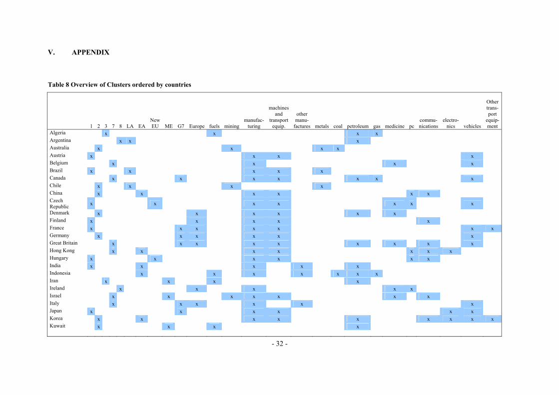
- 32 -

V. APPENDIX

Table 8 Overview of Clusters ordered by countries

1 2 3 7 8 LA EA New EU ME G7 Europe fuels mining

manufac-turing

machines and

transport equip.

other manu-

factures metals coal petroleum gas medicine pccommu-nications

electro-nics vehicles

Other trans-port

equip-ment

Algeria x x x x Argentina x x x Australia x x x x Austria x x x x Belgium x x x x Brazil x x x x x Canada x x x x x x x Chile x x x x China x x x x x x Czech Republic x x x x x x x

Denmark x x x x x x Finland x x x x x France x x x x x x x Germany x x x x x x Great Britain x x x x x x x x x Hong Kong x x x x x x x Hungary x x x x x x India x x x x x Indonesia x x x x x x x Iran x x x x Ireland x x x x x Israel x x x x x x x Italy x x x x x x Japan x x x x x x Korea x x x x x x x x x Kuwait x x x x

- 33 -

1 2 3 7 8 LA EA New EU ME G7 Europe fuels mining

manufac-turing

machines and

transport equip.

other manu-

factures metals coal petroleum gas medicine pccommu-nications

electro-nics vehicles

Other trans-port

equip-ment

Malaysia x x x x x x x x Mexico x x x x x x x Netherlands x x x x x x Nigeria x x x Norway x x x x x Philippines x x x x x x Poland x x x x x Portugal x x x x x Russia x x x x Saudi Arabia x x x x

Singapore x x x x x x x x Slovak Republic x x x x x x x

South Africa x x x x x x

Spain x x x x x Sweden x x x x x x x Switzerland x x x Thailand x x x x x x Turkey x x x Ukraine x x x x United Arab Emirates x x x x

United States x x x x x x

Venezuela x x x x Viet Nam x x x x

Note: The table provides information on the clustering of countries according to a series of characteristics, e.g. linked to their export specialization or the specific behavior of their trade elasticity. Description of the clusters: For the clusters 1,2,3,7 and 8 the countries were grouped together according to the consecutive patterns observed for the estimated elasticities of total imports to GDP through three sub-period: 1980-1990, 1990-2000, and 2000-2008: Cluster 1: countries with an increasing elasticity over the full sample, which

- 34 -

overshoots in the middle of the sample; cluster 2: countries with an increasing elasticity over the full sample; cluster 3: countries with an increasing elasticity over the full sample, but with a drop in the middle of the sample; cluster 7: countries with a decreasing elasticity over the full sample, but with an increase in the middle of the sample; and cluster 8: countries with a decreasing elasticity over the full sample (albeit the total number of possible clusters is 9, some of them were empty); LA = Latin America; EA = Emerging Asia; New EU = New Member Countries of the EU; ME = Middle East; G7 = G7-Countries; Europe = European Countries; fuels = fuels; mining = ores, metals, precious stones and non-monetary gold; manufacturing = manufactured goods; machines and transport equip. = machinery and transport equipment; other manufactures = other manufactured goods; metals = metalliferous ores and metal scrap; coal = coal, coke and briquettes; petroleum = petroleum, petroleum products and related materials; gas = gas, natural and manufactured; medicine = medicinal and pharmaceutical products; pc = office machines and automatic data-processing machines; communications = telecommunications and sound-recording and reproducing apparatus and equipment; electronics = electrical machinery, apparatus and appliances, n.e.s., and electrical parts thereof; vehicles = road vehicles (including air-cushion vehicles); other transport equipment = other transport equipment.

- 35 -

Table 9: Overview of Countries in each cluster

Clusters by observed elasticity patterns Cluster 1 Austria, Brazil, Czech Republic, Finland, France, Hungary, India,

Japan, Poland, Slovak Republic, South Africa, Sweden, Turkey Cluster 2 Australia, Chile, China, Denmark, Germany, Korea, Kuwait,

Malaysia, Netherlands, Nigeria, Norway, Portugal, Russia, Saudi Arabia, United Arab Emirates, Venezuela, Viet Nam

Cluster 3 Algeria, Iran, Singapore, Thailand, Ukraine Custer 7 Belgium, Canada, Great Britain, Hong Kong, Israel, Italy,

Philippines, Switzerland, USA Cluster 8 Argentina, Ireland, Mexico, Spain Clusters by export specialization Fuel exporters Algeria, Indonesia, Iran, Kuwait, Nigeria, Norway, Russia, Saudi

Arabia, United Arab Emirates, Venezuela Ores, metals, precious stones and non-monetary gold exporters

Australia, Chile, Israel, South Africa

Manufactured goods exporters Austria, Belgium, Brazil, Canada, China, Czech Republic, Denmark, Finland, France, Germany, Great Britain, Hong Kong, Hungary, India, Indonesia, Ireland, Israel, Italy, Japan, Korea, Malaysia, Mexico, Netherlands, Philippines, Poland, Portugal, Singapore, Slovak Republic, South Africa, Spain, Sweden, Switzerland, Thailand, Turkey, Ukraine, USA, Viet Nam

Machinery and transport equipment exporters

Austria, Brazil, Canada, China, Czech Republic, Denmark, Finland, France, Germany, Great Britain, Hong Kong, Hungary, Israel, Japan, Korea, Malaysia, Mexico, Netherlands, Philippines, Poland, Singapore, Slovak Republic, South Africa, Spain, Sweden, Thailand, USA

Other manufactured goods exporters

India, Indonesia, Italy, Portugal, Switzerland, Turkey, Ukraine, Viet Nam

Clusters by export specialization (export product) Metalliferous ores and metal scrap exporters

Australia, Brazil, Chile

Coal, coke and briquettes exporters

Australia, Indonesia, South Africa

Petroleum, petroleum products and related materials exporters

Algeria, Argentina, Canada, Denmark, Great Britain, India, Indonesia, Iran, Korea, Kuwait, Malaysia, Mexico, Netherlands, Nigeria, Norway, Russia, Saudi Arabia, Singapore, Slovak Republic, Ukraine, United Arab Emirates, Venezuela, Viet Nam

Gas, natural and manufactured, exporters

Algeria, Canada, Indonesia, Norway, Russia

Medicinal and pharmaceutical products exporters

Belgium, Czech Republic, Denmark, Great Britain, Ireland, Israel, Sweden

Office machines and automatic data-processing machines exporters

China, Czech Republic, Hong Kong, Hungary, Ireland, Malaysia, Netherlands, Philippines, Singapore, Thailand

Telecommunications and sound-recording and reproducing apparatus and equipment exporters

China, Finland, Great Britain, Hong Kong, Hungary, Israel, Korea, Malaysia, Mexico, Singapore, Slovak Republic, Sweden

- 36 -

Electrical machinery, apparatus and appliances, n.e.s., and electrical parts thereof exporters

Hong Kong, Japan, Korea, Malaysia, Philippines, Singapore, Thailand, USA

Road vehicles (including air-cushion vehicles) exporters

Austria, Belgium, Canada, Czech Republic, France, Germany, Great Britain, Italy, Japan, Korea, Mexico, Poland, Portugal, Slovak Republic, South Africa, Spain, Sweden

Other transport equipment exporters

France, Korea, USA

Clusters by region Latin America Argentina, Brazil, Chile, Mexico, Venezuela Emerging Asia China, Hong-Kong, India, Indonesia, Korea, Malaysia,

Philippines, Singapore, Thailand New EU-Member States Czech Republic, Hungary, Poland, Slovak Republic Middle East Iran, Israel, Kuwait, Saudi Arabia, United Arab Emirates G7-Countries Canada, France, Germany, Great Britain, Italy, Japan, USA Western European Countries Denmark, Finland, France, Germany, Great Britain, Ireland, Italy,

Netherlands, Norway, Portugal, Spain, Sweden Note: The table provides information on the countries included in each cluster. Source: Classification based on authors' calculations and UNCTAD (2008).

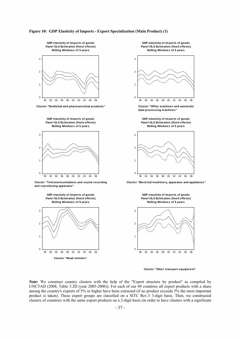
- 37 -

Figure 10: GDP Elasticity of Imports - Export Specialization (Main Product) (1)

0

1

2

3

90 92 94 96 98 00 02 04 06 08

GDP elasticity of im ports of goodsPanel OLS Estim ation (fixed effects)

Rolling Window s of 5 years

Cluster "Medicinal and pharm aceutical products"

0

1

2

3

90 92 94 96 98 00 02 04 06 08



Cluster "Office m achines and autom aticdata-processing m achines"

0

1

2

3

90 92 94 96 98 00 02 04 06 08



Cluster "Telecom m unications and sound-recordingand reproducing apparatus"

0

1

2

3

90 92 94 96 98 00 02 04 06 08



Cluster "Electrical m achinery, apparatus and appliances"

0

1

2

3

90 92 94 96 98 00 02 04 06 08



Cluster "Road vehicles"

0

1

2

3

90 92 94 96 98 00 02 04 06 08



Cluster "Other transport equipm ent"

Note: We construct country clusters with the help of the "Export structure by product" as compiled by UNCTAD (2008, Table 3.2D (year 2005-2006)). For each of our 49 countries all export products with a share among the country's exports of 5% or higher have been extracted (if no product exceeds 5% the most important product is taken). These export groups are classified on a SITC Rev.3 3-digit basis. Then, we constructed clusters of countries with the same export products on a 2-digit basis (in order to have clusters with a significant

- 38 -

number of countries); and made the analysis with those clusters that comprise at least three countries. The analysis was conducted with the following export-product-country groups: Metalliferous ores and metal scrap exporters; coal, coke and briquettes exporters; petroleum, petroleum products and related materials exporters; gas, natural and manufactured, exporters; medicinal and pharmaceutical products exporters; office machines and automatic data-processing machines exporters; telecommunications and sound-recording and reproducing apparatus and equipment exporters; electrical machinery, apparatus and appliances, n.e.s., and electrical parts thereof exporters; road vehicles (including air-cushion vehicles) exporters; and other transport equipment exporters.

Source: Authors' calculations. Figure 11: GDP Elasticity of Imports – Export Specialization (Main Product) (2)

-1

0

1

2

3

4

90 92 94 96 98 00 02 04 06 08



Cluster "Metalliferous ores and metal scrap"

-1

0

1

2

3

4

90 92 94 96 98 00 02 04 06 08



Cluster "Coal, coke and briquettes"

-1

0

1

2

3

4

90 92 94 96 98 00 02 04 06 08



Cluster "Petroleum, petroleum products and related materials"

-1

0

1

2

3

4

90 92 94 96 98 00 02 04 06 08



Cluster "Gas, natural and manufactured"

Note: See Note to Figure 8. Source: Authors' calculations.

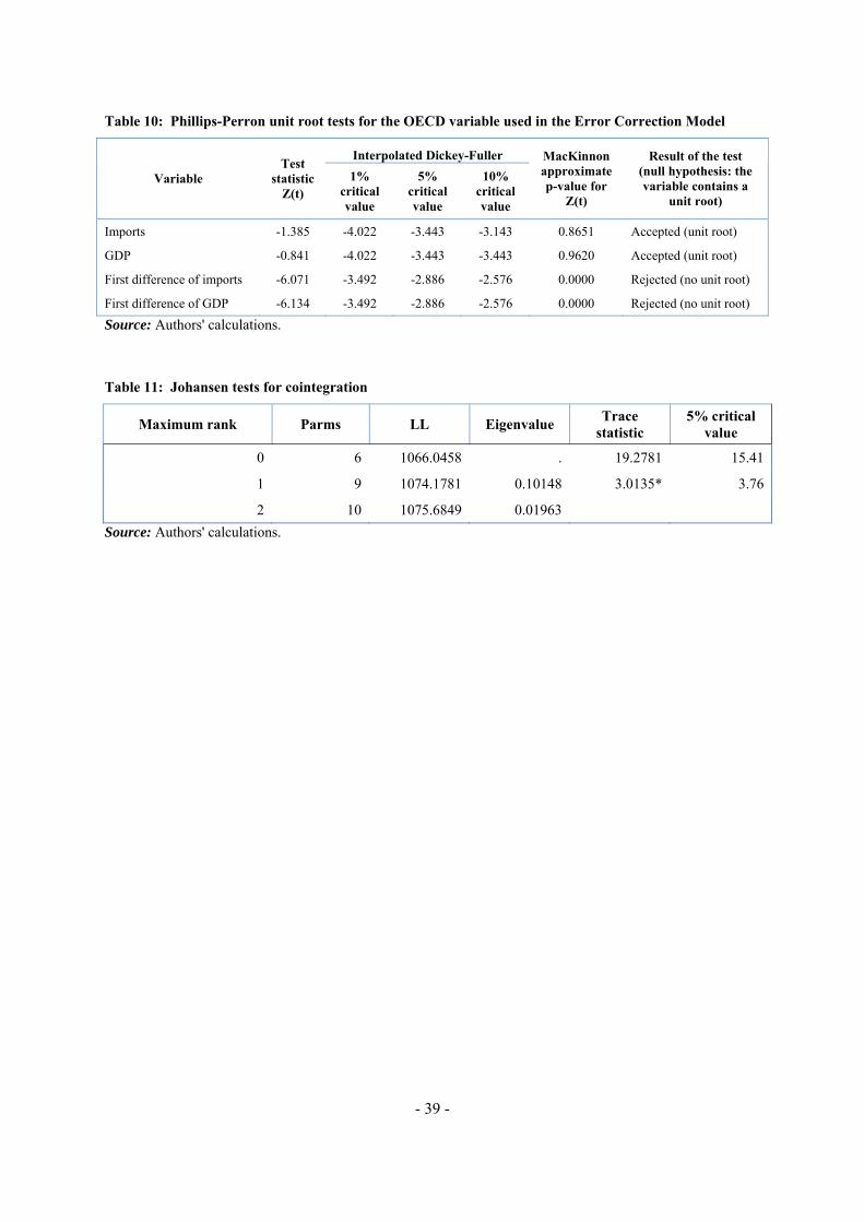
- 39 -

Table 10: Phillips-Perron unit root tests for the OECD variable used in the Error Correction Model

Interpolated Dickey-Fuller

Variable Test

statistic Z(t)

1% critical value

5% critical value

10% critical value

MacKinnon approximate p-value for

Z(t)

Result of the test (null hypothesis: the variable contains a

unit root)

Imports -1.385 -4.022 -3.443 -3.143 0.8651 Accepted (unit root)

GDP -0.841 -4.022 -3.443 -3.443 0.9620 Accepted (unit root)

First difference of imports -6.071 -3.492 -2.886 -2.576 0.0000 Rejected (no unit root)

First difference of GDP -6.134 -3.492 -2.886 -2.576 0.0000 Rejected (no unit root)

Source: Authors' calculations. Table 11: Johansen tests for cointegration

Maximum rank Parms LL Eigenvalue Trace statistic

5% critical value

0 6 1066.0458 . 19.2781 15.41

1 9 1074.1781 0.10148 3.0135* 3.76

2 10 1075.6849 0.01963 Source: Authors' calculations.

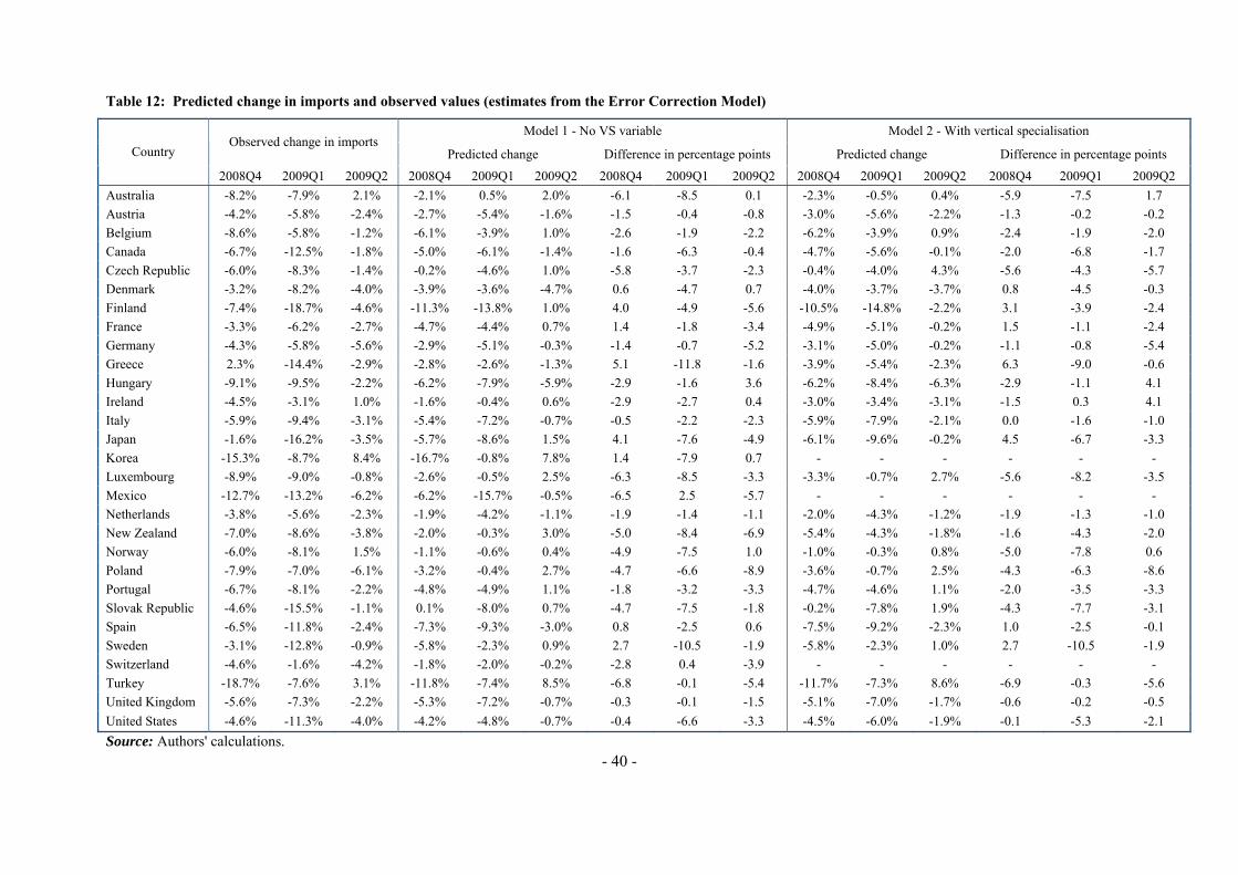
- 40 -

Table 12: Predicted change in imports and observed values (estimates from the Error Correction Model)

Model 1 - No VS variable Model 2 - With vertical specialisation Observed change in imports

Predicted change Difference in percentage points Predicted change Difference in percentage points Country

2008Q4 2009Q1 2009Q2 2008Q4 2009Q1 2009Q2 2008Q4 2009Q1 2009Q2 2008Q4 2009Q1 2009Q2 2008Q4 2009Q1 2009Q2 Australia -8.2% -7.9% 2.1% -2.1% 0.5% 2.0% -6.1 -8.5 0.1 -2.3% -0.5% 0.4% -5.9 -7.5 1.7 Austria -4.2% -5.8% -2.4% -2.7% -5.4% -1.6% -1.5 -0.4 -0.8 -3.0% -5.6% -2.2% -1.3 -0.2 -0.2 Belgium -8.6% -5.8% -1.2% -6.1% -3.9% 1.0% -2.6 -1.9 -2.2 -6.2% -3.9% 0.9% -2.4 -1.9 -2.0 Canada -6.7% -12.5% -1.8% -5.0% -6.1% -1.4% -1.6 -6.3 -0.4 -4.7% -5.6% -0.1% -2.0 -6.8 -1.7 Czech Republic -6.0% -8.3% -1.4% -0.2% -4.6% 1.0% -5.8 -3.7 -2.3 -0.4% -4.0% 4.3% -5.6 -4.3 -5.7 Denmark -3.2% -8.2% -4.0% -3.9% -3.6% -4.7% 0.6 -4.7 0.7 -4.0% -3.7% -3.7% 0.8 -4.5 -0.3 Finland -7.4% -18.7% -4.6% -11.3% -13.8% 1.0% 4.0 -4.9 -5.6 -10.5% -14.8% -2.2% 3.1 -3.9 -2.4 France -3.3% -6.2% -2.7% -4.7% -4.4% 0.7% 1.4 -1.8 -3.4 -4.9% -5.1% -0.2% 1.5 -1.1 -2.4 Germany -4.3% -5.8% -5.6% -2.9% -5.1% -0.3% -1.4 -0.7 -5.2 -3.1% -5.0% -0.2% -1.1 -0.8 -5.4 Greece 2.3% -14.4% -2.9% -2.8% -2.6% -1.3% 5.1 -11.8 -1.6 -3.9% -5.4% -2.3% 6.3 -9.0 -0.6 Hungary -9.1% -9.5% -2.2% -6.2% -7.9% -5.9% -2.9 -1.6 3.6 -6.2% -8.4% -6.3% -2.9 -1.1 4.1 Ireland -4.5% -3.1% 1.0% -1.6% -0.4% 0.6% -2.9 -2.7 0.4 -3.0% -3.4% -3.1% -1.5 0.3 4.1 Italy -5.9% -9.4% -3.1% -5.4% -7.2% -0.7% -0.5 -2.2 -2.3 -5.9% -7.9% -2.1% 0.0 -1.6 -1.0 Japan -1.6% -16.2% -3.5% -5.7% -8.6% 1.5% 4.1 -7.6 -4.9 -6.1% -9.6% -0.2% 4.5 -6.7 -3.3 Korea -15.3% -8.7% 8.4% -16.7% -0.8% 7.8% 1.4 -7.9 0.7 - - - - - - Luxembourg -8.9% -9.0% -0.8% -2.6% -0.5% 2.5% -6.3 -8.5 -3.3 -3.3% -0.7% 2.7% -5.6 -8.2 -3.5 Mexico -12.7% -13.2% -6.2% -6.2% -15.7% -0.5% -6.5 2.5 -5.7 - - - - - - Netherlands -3.8% -5.6% -2.3% -1.9% -4.2% -1.1% -1.9 -1.4 -1.1 -2.0% -4.3% -1.2% -1.9 -1.3 -1.0 New Zealand -7.0% -8.6% -3.8% -2.0% -0.3% 3.0% -5.0 -8.4 -6.9 -5.4% -4.3% -1.8% -1.6 -4.3 -2.0 Norway -6.0% -8.1% 1.5% -1.1% -0.6% 0.4% -4.9 -7.5 1.0 -1.0% -0.3% 0.8% -5.0 -7.8 0.6 Poland -7.9% -7.0% -6.1% -3.2% -0.4% 2.7% -4.7 -6.6 -8.9 -3.6% -0.7% 2.5% -4.3 -6.3 -8.6 Portugal -6.7% -8.1% -2.2% -4.8% -4.9% 1.1% -1.8 -3.2 -3.3 -4.7% -4.6% 1.1% -2.0 -3.5 -3.3 Slovak Republic -4.6% -15.5% -1.1% 0.1% -8.0% 0.7% -4.7 -7.5 -1.8 -0.2% -7.8% 1.9% -4.3 -7.7 -3.1 Spain -6.5% -11.8% -2.4% -7.3% -9.3% -3.0% 0.8 -2.5 0.6 -7.5% -9.2% -2.3% 1.0 -2.5 -0.1 Sweden -3.1% -12.8% -0.9% -5.8% -2.3% 0.9% 2.7 -10.5 -1.9 -5.8% -2.3% 1.0% 2.7 -10.5 -1.9 Switzerland -4.6% -1.6% -4.2% -1.8% -2.0% -0.2% -2.8 0.4 -3.9 - - - - - - Turkey -18.7% -7.6% 3.1% -11.8% -7.4% 8.5% -6.8 -0.1 -5.4 -11.7% -7.3% 8.6% -6.9 -0.3 -5.6 United Kingdom -5.6% -7.3% -2.2% -5.3% -7.2% -0.7% -0.3 -0.1 -1.5 -5.1% -7.0% -1.7% -0.6 -0.2 -0.5 United States -4.6% -11.3% -4.0% -4.2% -4.8% -0.7% -0.4 -6.6 -3.3 -4.5% -6.0% -1.9% -0.1 -5.3 -2.1 Source: Authors' calculations.