international product life cycles, trade and development ... · international product life cycles,...
TRANSCRIPT

International product life cycles, trade and developmentstages
David Audretsch1 • Mark Sanders2 • Lu Zhang3
� The Author(s) 2017. This article is an open access publication
Abstract In this paper we first propose a proxy for early stage activity in a country’s
exports based on product life cycle theory. Employing a conditional latent class model, we
then examine the relationship between this measure and economic growth for 93 countries
during the period 1988–2005. We find that the impact of early stage activity differs across
three clusters of countries. And we find that GDP levels can predict the cluster and the sign
of the coefficient in a non-linear manner. In the richest countries, exporting products that
are in an early stage of their product life cycle is associated with higher growth rates. In
contrast, we find a cluster of middle income countries with high growth rates that grow
faster by exporting more mature products that are in the later stages of their life cycle.
Finally, early stage activity has no significant impact on growth in the cluster of the
poorest, developing countries. Countries in early stages of development should focus on
acquiring market share in mature markets with routine technologies whereas emerging
economies face the challenge of at some point switching from copying mature to inventing
new products as they approach the global technology frontier. At that frontier they must
join the advanced economies who specialise in early stage innovative products to stay
ahead of increasing competition from abroad.
& Lu [email protected]
David [email protected]
Mark [email protected]
1 Institute for Development Strategies, Indiana University Bloomington, 1315 E. 10th Street, SPEA201, Bloomington, IN 47405, USA
2 Utrecht University School of Economics, Utrecht University, P.O. Box 80125, 3508 TC Utrecht,The Netherlands
3 Sustainable Finance Lab, Utrecht University, P.O.Box 80125, 3508 TC Utrecht, The Netherlands
123
J Technol TransfDOI 10.1007/s10961-017-9588-6
Keywords Product life cycles � Trade � Maturity � Economic growth � Conditionallatent class model
JEL Classification F14 � O00
1 Introduction
Ever since Adam Smith linked specialisation and trade to the wealth of nations, trade and
competitiveness in international markets has been considered a key driver for development
and national well being. For that reason trade has been subject of intense academic and
policy interest. Using strategic trade- and industrial policies governments across the world
try to push their countries up in the league of nations. It has been found that specialising in
the ‘‘right’’ products and markets helps countries move ahead, whereas a focus on the
‘‘wrong’’ export bundle can keep a nation trapped in poverty (e.g. Redding 2002; Bensi-
doun et al. 2002; Hausmann et al. 2007). But despite the fact that much of the academic
literature on this topic stresses the dynamic nature of comparative advantage, to date it fails
to consider that ‘‘right’’ and ‘‘wrong’’ are not absolutes. In this paper we argue that the
‘‘right’’ products in emerging countries may well be different from the ‘‘right’’ products in
advanced economies. Moreover, the bundle of ‘‘right’’ and ‘‘wrong’’ products will change
over time as products mature over their life cycle. It makes quite a difference if you, for
example, specialise in video cassette recorders (VCRs) in the early 1980s or in the late
2000s. And it matters a lot also if you do so when you are an emerging economy starting to
industrialise or when you are an advanced country at the global technology frontier.
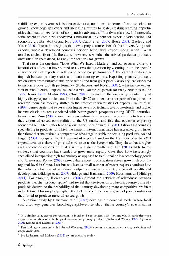
Taking a more dynamic approach to specialisation will go a long way in explaining
some of the most salient features of global economic development in recent decades. This
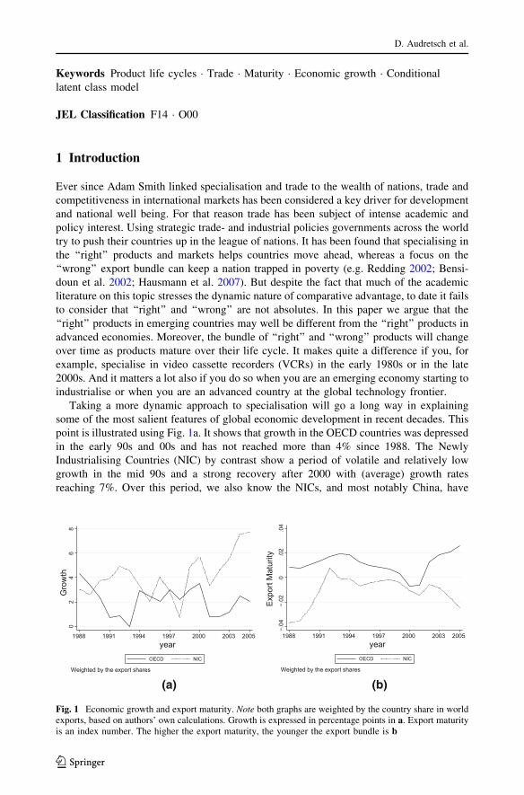
point is illustrated using Fig. 1a. It shows that growth in the OECD countries was depressed
in the early 90s and 00s and has not reached more than 4% since 1988. The Newly
Industrialising Countries (NIC) by contrast show a period of volatile and relatively low
growth in the mid 90s and a strong recovery after 2000 with (average) growth rates
reaching 7%. Over this period, we also know the NICs, and most notably China, have
02
46
8G
row
th
1988 1991 1994 1997 2000 2003 2005year
OECD NIC
Weighted by the export shares
−.04
−.02
0.0
2.0
4
Exp
ort M
atur
ity
1988 1991 1994 1997 2000 2003 2005year
OECD NIC
Weighted by the export shares
(a) (b)
Fig. 1 Economic growth and export maturity. Note both graphs are weighted by the country share in worldexports, based on authors’ own calculations. Growth is expressed in percentage points in a. Export maturityis an index number. The higher the export maturity, the younger the export bundle is b
D. Audretsch et al.
123
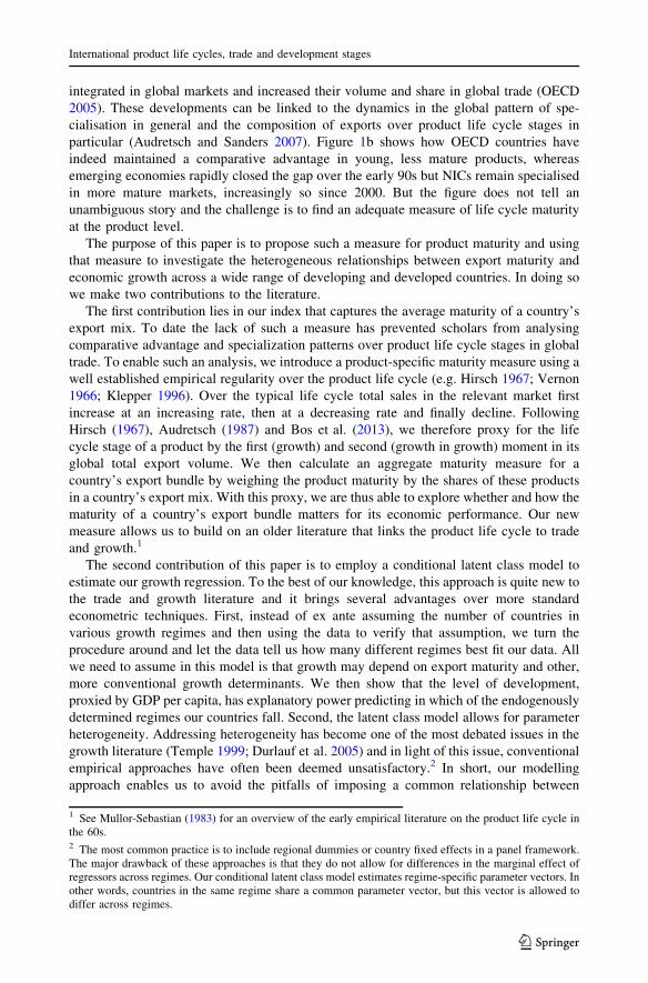
integrated in global markets and increased their volume and share in global trade (OECD
2005). These developments can be linked to the dynamics in the global pattern of spe-
cialisation in general and the composition of exports over product life cycle stages in
particular (Audretsch and Sanders 2007). Figure 1b shows how OECD countries have
indeed maintained a comparative advantage in young, less mature products, whereas
emerging economies rapidly closed the gap over the early 90s but NICs remain specialised
in more mature markets, increasingly so since 2000. But the figure does not tell an
unambiguous story and the challenge is to find an adequate measure of life cycle maturity
at the product level.
The purpose of this paper is to propose such a measure for product maturity and using
that measure to investigate the heterogeneous relationships between export maturity and
economic growth across a wide range of developing and developed countries. In doing so
we make two contributions to the literature.
The first contribution lies in our index that captures the average maturity of a country’s
export mix. To date the lack of such a measure has prevented scholars from analysing
comparative advantage and specialization patterns over product life cycle stages in global
trade. To enable such an analysis, we introduce a product-specific maturity measure using a
well established empirical regularity over the product life cycle (e.g. Hirsch 1967; Vernon
1966; Klepper 1996). Over the typical life cycle total sales in the relevant market first
increase at an increasing rate, then at a decreasing rate and finally decline. Following
Hirsch (1967), Audretsch (1987) and Bos et al. (2013), we therefore proxy for the life
cycle stage of a product by the first (growth) and second (growth in growth) moment in its
global total export volume. We then calculate an aggregate maturity measure for a
country’s export bundle by weighing the product maturity by the shares of these products
in a country’s export mix. With this proxy, we are thus able to explore whether and how the
maturity of a country’s export bundle matters for its economic performance. Our new
measure allows us to build on an older literature that links the product life cycle to trade
and growth.1
The second contribution of this paper is to employ a conditional latent class model to
estimate our growth regression. To the best of our knowledge, this approach is quite new to
the trade and growth literature and it brings several advantages over more standard
econometric techniques. First, instead of ex ante assuming the number of countries in
various growth regimes and then using the data to verify that assumption, we turn the
procedure around and let the data tell us how many different regimes best fit our data. All
we need to assume in this model is that growth may depend on export maturity and other,
more conventional growth determinants. We then show that the level of development,
proxied by GDP per capita, has explanatory power predicting in which of the endogenously
determined regimes our countries fall. Second, the latent class model allows for parameter
heterogeneity. Addressing heterogeneity has become one of the most debated issues in the
growth literature (Temple 1999; Durlauf et al. 2005) and in light of this issue, conventional
empirical approaches have often been deemed unsatisfactory.2 In short, our modelling
approach enables us to avoid the pitfalls of imposing a common relationship between
1 See Mullor-Sebastian (1983) for an overview of the early empirical literature on the product life cycle inthe 60s.2 The most common practice is to include regional dummies or country fixed effects in a panel framework.The major drawback of these approaches is that they do not allow for differences in the marginal effect ofregressors across regimes. Our conditional latent class model estimates regime-specific parameter vectors. Inother words, countries in the same regime share a common parameter vector, but this vector is allowed todiffer across regimes.
International product life cycles, trade and development stages
123
export maturity and growth for all countries but yields results that are comparable across
countries and time. Our approach is closely related to recent studies that apply conditional
latent class (or finite mixture) models to examine the the heterogeneity of growth and
convergence patterns across countries.3
In our study we apply our method to Statistics Canada’s version of the UN-COM-
TRADE database that contains the export data on 427 Standard International Trade
Classification (SITC) four-digit products for 93 countries over the period 1988–2005. This
database gives us the opportunity to zoom in on relatively narrowly defined groups of
products and generalise trade patterns across more countries than most studies to date. We
thus propose a simple measure of product maturity in the global market and then link the
overall average maturity of a country’s export portfolio to their economic growth
performance.
Our results are easy to summarise. We find that developed countries (with high GDP per
capita) are exporting products in the early stages of their (global) life cycle, whereas the
opposite is true for developing countries. In addition, we find evidence for the existence of
three quite distinct growth regimes. For the advanced countries’ regime, exporting new and
innovate products is associated with higher economic growth, whereas this relationship is
insignificant for the developing countries’ (lowest GDP per capita) regime. In stark con-
trast, we identify an emerging countries’ regime where exporting more mature products
appears to be associated with more rapid growth. These findings have important impli-
cations for trade and economic development theory and policies. Notably, our results
suggests we can look at specialization and dynamic comparative advantage as an advan-
tage in exporting goods and services in a given stage of the life cycle. Advanced economies
do not have a comparative advantage in computers or machinery, but in early stage
products. Likewise, emerging economies have a comparative advantage in mature prod-
ucts. The early stage products of a decade ago, however, are today’s mature products. And
product classes (i.e. telephones) can be rejuvenated through innovation. Taking such an
approach to economic development has clear implications for policy. Advanced economies
should focus their efforts and resources on shifting out the global technology frontier,
whereas emerging economies will prosper by capturing existing, mature markets.
The remainder of the paper proceeds as follows. First we position our paper in the
relevant literatures on trade and growth in Sect. 2. In Sect. 3 we present a stylised model of
trade and product life cycles to derive our key hypothesis. Note that this paper does not aim
to make a theoretical contribution and the model is merely presented to provide a
framework in which to interpret our empirical results. In Sect. 4, we develop our maturity
proxy and discuss our data and estimation strategies. The empirical results are then pre-
sented in Sect. 5. And Sect. 6 discusses the implications of our paper and concludes.
3 Specifically, Paap et al. (2005) apply a latent class analysis to sort a number of developing countriesaccording to their average growth rates over the period 1961–2000. Alfo et al. (2008) develop a mixture ofcross-sectional growth regression to uncover multiple regimes of per capita income convergence across EUregions for the period 1980–2002. Owen et al. (2009) apply a conditional finite mixture model based on thesimilarity of the conditional distribution of growth rates for a broad set of countries for the period1970–2000, and find evidence of two distinct clubs, each with its own distinctive growth dynamics andinstitutional quality is a good predictor of the club membership. Bos et al. (2010) estimate a latent classproduction frontier and uncovers three different growth regimes using human capital, openness to trade,financial development, and the primary sector share as regime predictors for a sample of 77 countries duringthe period 1970–2000. Vaio and Enflo (2011) support that growth patterns were segmented in two world-wide regimes, the one characterised by convergence in per capita income, and the other by divergence basedon a sample of 64 countries over a very long horizon 1870–2003. Owen and Videras (2012) use latent classanalysis to characterise development experiences of countries by taking into account the quality of growth.
D. Audretsch et al.
123
2 Literature review
Our paper builds on recent advances in two long traditions in the literature. The first strand,
pioneered by Vernon (1966), applies stylised life cycle models to explain the shift of
dynamic comparative advantages and the evolvement of trade patterns over time (Hirsch
1967; Krugman 1979; Jensen and Thursby 1986; Kellman and Landau 1984; Dollar 1986;
Flam and Helpman 1987; Grossman and Helpman 1991; Lai 1995). An important pre-
diction in this line of literature is that developing countries will increasingly compete in
those products that reach the later stages of the product life cycle, implying that the
advanced economies must ‘‘run to stand still’’ (Krugman 1979). A steady flow of new
product innovations is necessary to maintain international income differentials. In these
models the assumed relative abundance of cheap, unskilled labour in the less developed
South is the source of a dynamic comparative advantage in copying mature products and
technologies from the more advanced North. If, in such a context, globalisation and trade
integration imply that populous developing economies enter global market competition,
then advanced economies experience a shift of their comparative advantage towards
products that are in the earliest stages of the product life cycle (see e.g. Lai 1995;
Audretsch and Sanders 2007).
The second strand of literature relevant to our work extensively documents the effect of
trade, and more specifically exports, on economic growth. The vast bulk of the early
empirical literature asks: ‘‘Do Exports Matter?’’.4 Most of these studies include either a
measure of export (growth) or trade openness in a standard regression framework covering
a wide range of countries, time periods and using a variety of estimation techniques.
Consistent with the difficulties in establishing robust empirical evidence linking growth to
fundamentals in general (Temple 1999; Durlauf et al. 2005), the evidence is rather mixed.
Some find a significant positive relationship between export (growth) and per capita GDP
growth, while others caution us not to assign the direction of causality (Rodriguez and
Rodrik 2001). An interesting contribution by Moschos (1989) hinted at the existence of
different regimes in the relationship between exports and growth. A salient feature of this
literature is that the measure of export/trade openness is typically broadly defined. As a
result, the channels through which international trade influences economic growth remain
unclear and possible heterogeneity over different development stages remains hidden.
A number of studies do examine the relationship between the structure of exports and
long-term economic performance in more detail and asks: ‘‘How do Exports Matter?’’.5 In
particular, this literature has focused on the relationship between export diversification and
growth (E.g. de Pineres and Ferrantino 1997). Export diversification is widely seen as a
desirable trade objective in promoting economic growth (Herzer and Nowak-Lehnmann
2006). Diversification makes countries less vulnerable to adverse terms of trade shocks. By
4 This literature is massive. Giles and Williams (2000) provides a comprehensive survey of more than 150papers that test the export-led growth hypothesis alone. Singh (2010) provides a recent survey of a growingbody of studies that explore linkages between trade openness and growth.5 The structure of imports may have direct impact on economic performance as well. Earlier studies showthat imports of quality foreign capital goods serves as a means to acquire foreign technology through reverseengineering (Connolly 1999). Lee (1995) and Lewer and Berg (2003) find that capital-importing countriesbenefit from trade because trade causes the cost of capital to fall, where Schneider (2005) shows that hightechnology imports matter for growth. However, others do not reveal any significant role for the compositionof imports in economic growth (An and Iyigun 2004; Worz 2005). In line with recent papers that analyse theimportance of export structure for better economic performance, this paper focuses on the export side andleave the import side for future research.
International product life cycles, trade and development stages
123
stabilising export revenues it is then easier to channel positive terms of trade shocks into
growth, knowledge spillovers and increasing returns to scale, creating learning opportu-
nities that lead to new forms of comparative advantage.6 In a dynamic growth framework,
some recent studies have uncovered a non-linear link between export diversification and
economic growth (Aditya and Roy 2007; Cadot et al. 2007; Hesse 2008; Xuefeng and
Yasar 2016). The main insight is that developing countries benefit from diversifying their
exports, whereas developed countries perform better with export specialisation.7 What
remains unclear from this literature, however, is whether the mix of particular products,
diversified or specialised, has any implications for growth.
That raises the question: ‘‘Does What We Export Matter?’’ and our paper is close to a
handful of studies that have started to address that question by zooming in on the specific
characteristics of exports in relation to economic performance.8 The earliest studies dis-
tinguish between primary sector and manufacturing exports. Exporting primary products,
which suffer from unfavourable price trends and from great price variability, are suspected
to associate poor growth performance (Rodriguez and Rodrik 2001), whereas the expan-
sion of manufactured exports has been a vital source of growth for many countries (Cline
1982; Ranis 1985; Martin 1993; Cline 2010). Thanks to the increasing availability of
highly disaggregated trade data, first in the OECD and then for other parts of the globe, the
research focus has recently shifted to the product characteristics of exports. Dalum et al.
(1999) demonstrate that exports with higher levels of technological opportunity and higher
income elasticities are associated with better growth prospects among OECD countries.
Feenstra and Rose (2000) developed a procedure to order countries according to how soon
they export advanced commodities to the US market and find that countries exporting
sooner to the United States tend to grow faster. Bensidoun et al. (2002) show that countries
specialising in products for which the share in international trade has increased grow faster
than those that maintained a comparative advantage in stable or declining products. An and
Iyigun (2004) compute the skill content of exports based on the US industry-wide R&D
expenditures as a share of gross sales revenue as the benchmark. They show that a higher
skill content of exports correlates with a higher growth rate. Lee (2011) adds to the
evidence that countries have tended to grow more rapidly when they have increasingly
specialised in exporting high-technology as opposed to traditional or low-technology goods
and Jarreau and Poncet (2012) shows that export sophistication drives growth also at the
regional level in China. Last but not least, a small number of recent papers examines how
the network structure of economic output influences a country’s overall wealth and
development (Hidalgo et al. 2007; Hidalgo and Hausmann 2009; Hausmann and Hidalgo
2011). For example, Hidalgo et al. (2007) present the network of relatedness between
products, i.e. the ‘‘product space’’ and reveal that the types of products a country currently
produces determine the probability of that country developing more competitive products
in the future. This may help explain the lack of economic convergence of poor countries as
they failed to produce more advanced goods.
A seminal study by Hausmann et al. (2007) develops a theoretical model where local
cost discovery generates knowledge spillovers to show that a country’s specialisation
6 In a similar vein, export concentration is found to be associated with slow growth, in particular whenexport concentration reflects the predominance of primary products (Sachs and Warner 1995; Gylfason2004; Klinger and Lederman 2006).7 This finding is consistent with Imbs and Wacziarg (2003) who find a similar pattern using production andemployment data.8 See Lederman and Maloney (2012) for an extensive review.
D. Audretsch et al.
123
pattern becomes partly indeterminate in the presence of such externalities. They conclude
from this that the mix of goods that a country produces may therefore have important
implications for economic growth and construct a product-specific sophistication measure
based on the income of the average exporter. They then test their hypothesis and find that
exporting more sophisticated products is positively associated with subsequent growth.
Building on these recent studies, we propose not to focus on a static product sophis-
tication measure but rather on a product’s life cycle stage in the global market. This has
important implications. With age, a product matures and becomes less sophisticated. In
addition, instead of postulating a development strategy for developing countries that should
shoot for the stars and export what the developed countries are exporting, we argue this
may not be optimal. Developing countries may lack the capability to produce complex
products (Indjikian and Siegel 2005).9 Therefore, our paper advocates a development
strategy that is better tuned to the development stages of countries. But let us first develop
our arguments a bit more formally.
3 A simple model adapted from Grossman and Helpman (1991)
Assume we can divide the world in two regions. And advanced ‘‘North’’ and emerging
‘‘South’’. Consumers in these two regions consume a variety of n goods, indexed by i
where utility in both regions is given by:
U ¼Xn
i¼0
cai ð1Þ
where U is a utility index, c is consumption and a is a parameter between 0 and 1. Global
demand for good i is then equal to:
cDi ¼ p1
a�1
i
E
Pð2Þ
where pi is the price of good i, E is global expenditure on consumption and P is a price
index defined as P �Pn
i¼0 pa
a�1
i . We assume that production follows a simple linear pro-
duction function in labor only, such that marginal production costs equal wages. Labor is
assumed immobile across regions but mobile across firms within a region, such that wages
are region specific and given to all firms. Firms produce a single variety i. We assume they
own tacit and proprietary knowledge that enables them to do so and consequently they are
price setters in their product market. Any product, however, can be imitated at some fixed
start-up cost. This implies we have four groups of products. New, i 2 AN;S and mature
i 2 MN;S products produced in North and South, respectively. We assume that new prod-
ucts require high skilled labor whereas mature products can also be produced with low
skilled labor. The profit maximisation problem for the producer is given by:
9 Indjikian and Siegel (2005) provide a comprehensive review on the impact of IT on economic perfor-mance in developed and developing countries. They find strong positive correlation between IT and eco-nomic performance in developed countries, but not in developing countries. They argue that two deficiencieshinder the use of IT in developing countries are the lack of knowledge of ‘‘best practice’’ and IT-skilledlabour force.
International product life cycles, trade and development stages
123
max :pi
pi ¼ piyi � wSCl
Si
subject to yi ¼ cDiyi ¼ lHi ; i 2 AC
yi ¼ lLi ; i 2 MC
ð3Þ
where C indexes the regions (N)orth and (S)outh and S the skill levels (H)igh and (L)ow. It
is straightforward to show that all firms will set their price equal to:
pi ¼1
awSC
ð4Þ
We assume for simplicity thatwLC
a \wHC such that all producers can set their prices freely.10
Let us first solve the model statically, that is, for a given portfolio of goods in the ranges
AN , MN , AS and MS. As costs are equal within these ranges, so are prices and demanded
quantities. Labor demand for high and low skilled labor in South and North can be set
equal to exogenous supply to yield:
LL�N ¼Xn
i¼0
ci piðwLNÞ
� �¼ MN
wLN
a
� � 1a�1E
P
LH�N ¼
Xn
i¼0
ci piðwHN Þ
� �¼ AN
wHN
a
� � 1a�1E
P
LL�S ¼Xn
i¼0
ci piðwLSÞ
� �¼ MS
wLS
a
� � 1a�1E
P
LH�S ¼
Xn
i¼0
ci piðwHS Þ
� �¼ AS
wHS
a
� � 1a�1E
P:
ð5Þ
We can now solve for equilibrium wages and express profits in product portfolio ranges,
exogenous labor supplies and parameters only.
pAN¼ ð1� aÞE
AN
A1�aN LH�
N
a
A1�aN LH�
Na þM1�a
N LL�Na þ A1�a
S LH�S
a þM1�aS LL�S
a
pMN¼ ð1� aÞE
MN
M1�aN LL�N
a
A1�aN LH�
Na þM1�a
N LL�Na þ A1�a
S LH�S
a þM1�aS LL�S
a
pAS¼ ð1� aÞE
AS
A1�aS LH�
S
a
A1�aN LH�
Na þM1�a
N LL�Na þ A1�a
S LH�S
a þM1�aS LL�S
a
pMS¼ ð1� aÞE
MS
M1�aS LL�S
a
A1�aN LH�
Na þM1�a
N LL�Na þ A1�a
S LH�S
a þM1�aS LL�S
a :
ð6Þ
Such that total profit in the economy adds up to ð1� aÞ times total expenditure. Also note
that the profit in any given product range is falling in all product ranges. These profits,
10 One should realise that, since advanced producers in the same or the other region can compete and will
produce when their marginal costs are below the market price. This caps the price of mature goods at wHC .
We assume here that this constraint is not binding, even for the mature product producers in the North
imitating their product from the South. We thus assume:wLS
a \[ wLN
a \wHS \[wH
N :
D. Audretsch et al.
123
however, are also strictly positive and provide an incentive to innovate (create new
products) and imitate (switch a product from advanced to mature). In this economy the
only long run source of economic growth is this expansion of the goods ranges. We can
show that a steady state can only exist when all goods ranges expand at a common growth
rate. Note from Eq. 6 that if all goods ranges expand at a common rate, g, we see that
profits in an individual firm will fall at a constant rate equal to the growth rate of
expenditure minus g. Setting the former to 0 by normalising expenditure to 1 we obtain �g
for the growth rate of profit. The value of a new firm in either goods range will be equal to
the discounted profit flow over the expected remaining lifetime of the firm. For mature
goods we assume this lifetime to be infinite and the value of a firm producing an mature
good in country C is:
VMCðtÞ ¼
Z 1
t
e�rspMCðsÞds ¼
Z 1
t
e�ðrþgÞspMCðtÞds ¼ pMC
ðtÞr þ g
: ð7Þ
For advanced goods it is slightly more complicated, as the profit flow ends when the
product is imitated. However, if we assume the expected flow probability of that happening
is constant in the steady state at h we can compute the value of a new firm as:
VACðtÞ ¼
Z 1
t
e�ðrþhÞspACðsÞds ¼
Z 1
t
e�ðrþhþgÞspACðtÞds ¼ pMC
ðtÞr þ hþ g
: ð8Þ
We endogenise innovation and imitation as in e.g. Grossman and Helpman (1991) and
Audretsch and Sanders (2007) by assuming R&D firms can employ R&D resources to
innovate according to:
_AC ¼ ACcMC
1�cRRC ð9Þ
where the dot signifies a time derivative and the Cobb–Douglas aggregate of AC and MC
represents the knowledge stock and 0:5\c\1 would imply more recent knowledge is
given more weight, while RRC is R&D resources allocated to the creation of new products.
Likewise we assume imitation takes place according to:
_MC ¼ ACdA�C
1�dRDC ð10Þ
where A�C is the range of imitable advanced products not in country C and so the relevant
knowledge base is a Cobb–Douglas aggregate of domestic and foreign imitable products
and 0:5\d\1 would imply it is easier to imitate from home. We can compute the
marginal value product of R&D resources in imitation and innovation by multiplying the
derivative of Eqs. (9) and (10) with respect to R&D labor by the value of a new or mature
firm in country C in Eqs. (8) and (7), respectively. Substitution for profits using Eq. (6) in
both countries and dividing the resulting expressions on each other we obtain:
r þ hþ g
r þ g¼ AN
�aþc�dASd�1MN
1�a�c LHN�LLN�
� �a
r þ hþ g
r þ g¼ AS
�aþc�dANd�1MS
1�a�c LHS �LLS�
� �að11Þ
as R&D arbitrage conditions for North and South respectively. This arbitrage condition
allows us to derive some comparative statics on the steady state, in which the left hand side
is equal for both regions. We then obtain:
International product life cycles, trade and development stages
123
LHNLLN
LLSLHS
� �aMN
MS
� �2ð1�dÞ¼ AN
MN
MS
AS
� ��1þa�cþ2d
ð12Þ
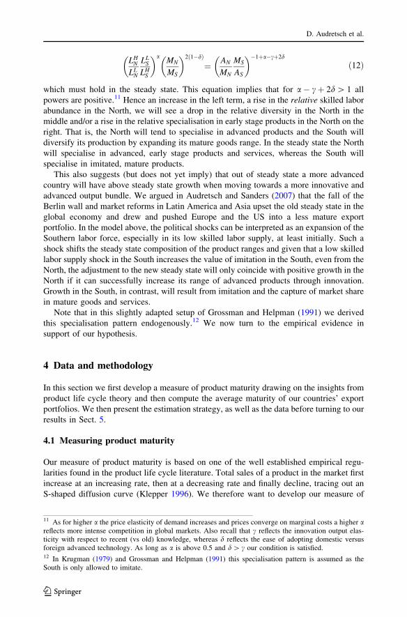
which must hold in the steady state. This equation implies that for a� cþ 2d[ 1 all
powers are positive.11 Hence an increase in the left term, a rise in the relative skilled labor
abundance in the North, we will see a drop in the relative diversity in the North in the
middle and/or a rise in the relative specialisation in early stage products in the North on the
right. That is, the North will tend to specialise in advanced products and the South will
diversify its production by expanding its mature goods range. In the steady state the North
will specialise in advanced, early stage products and services, whereas the South will
specialise in imitated, mature products.
This also suggests (but does not yet imply) that out of steady state a more advanced
country will have above steady state growth when moving towards a more innovative and
advanced output bundle. We argued in Audretsch and Sanders (2007) that the fall of the
Berlin wall and market reforms in Latin America and Asia upset the old steady state in the
global economy and drew and pushed Europe and the US into a less mature export
portfolio. In the model above, the political shocks can be interpreted as an expansion of the
Southern labor force, especially in its low skilled labor supply, at least initially. Such a
shock shifts the steady state composition of the product ranges and given that a low skilled
labor supply shock in the South increases the value of imitation in the South, even from the
North, the adjustment to the new steady state will only coincide with positive growth in the
North if it can successfully increase its range of advanced products through innovation.
Growth in the South, in contrast, will result from imitation and the capture of market share
in mature goods and services.
Note that in this slightly adapted setup of Grossman and Helpman (1991) we derived
this specialisation pattern endogenously.12 We now turn to the empirical evidence in
support of our hypothesis.
4 Data and methodology
In this section we first develop a measure of product maturity drawing on the insights from
product life cycle theory and then compute the average maturity of our countries’ export
portfolios. We then present the estimation strategy, as well as the data before turning to our
results in Sect. 5.
4.1 Measuring product maturity
Our measure of product maturity is based on one of the well established empirical regu-
larities found in the product life cycle literature. Total sales of a product in the market first
increase at an increasing rate, then at a decreasing rate and finally decline, tracing out an
S-shaped diffusion curve (Klepper 1996). We therefore want to develop our measure of
11 As for higher a the price elasticity of demand increases and prices converge on marginal costs a higher areflects more intense competition in global markets. Also recall that c reflects the innovation output elas-ticity with respect to recent (vs old) knowledge, whereas d reflects the ease of adopting domestic versusforeign advanced technology. As long as a is above 0.5 and d[ c our condition is satisfied.12 In Krugman (1979) and Grossman and Helpman (1991) this specialisation pattern is assumed as theSouth is only allowed to imitate.
D. Audretsch et al.
123
maturity at the product level by looking at the dynamics in market volume at the global
level. Following Audretsch (1987) and Bos et al. (2013), we characterise the life cycle
stage of a product using the first and second moment in its global export volume.
We calculate product maturity for each of the 427 SITC four-digit products over the
period 1988–2005 using global-level export data retrieved from the UN-COMTRADE
database. The problem with our real trade data is that we do not have the sales volumes for
individual products at more disaggregated levels. Instead we have four-digit product
classes in which still any number of different products, potentially all in different stages of
their respective life cycles, are being added together. However, it is important to note that
our product maturity measure captures the average life cycle stage of these product classes.
More importantly, our measure can correctly identify the rejuvenation of the product class
that is the result of replacing a mature with a new product. We demonstrate these features
of our measure through a simulation exercise below. The findings confirm that our measure
indeed captures the product life cycle stage in data we have generated ourselves and four-
digit product is the right product category for the purpose of this paper.
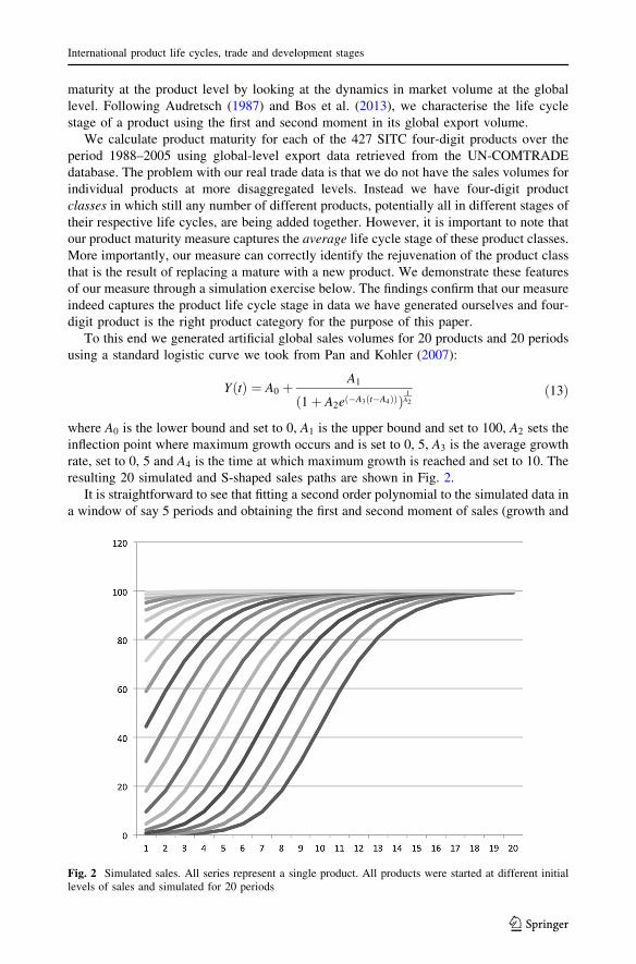
To this end we generated artificial global sales volumes for 20 products and 20 periods
using a standard logistic curve we took from Pan and Kohler (2007):
YðtÞ ¼ A0 þA1
1þ A2eð�A3ðt�A4ÞÞð Þ1A2
ð13Þ
where A0 is the lower bound and set to 0, A1 is the upper bound and set to 100, A2 sets the
inflection point where maximum growth occurs and is set to 0, 5, A3 is the average growth
rate, set to 0, 5 and A4 is the time at which maximum growth is reached and set to 10. The
resulting 20 simulated and S-shaped sales paths are shown in Fig. 2.
It is straightforward to see that fitting a second order polynomial to the simulated data in
a window of say 5 periods and obtaining the first and second moment of sales (growth and
Fig. 2 Simulated sales. All series represent a single product. All products were started at different initiallevels of sales and simulated for 20 periods
International product life cycles, trade and development stages
123
growth in growth) would be sufficient to characterise the product life cycle stage. Suppose
we estimate and compute:
lnðYtÞ ¼ c0 þ c1t þ c2t2 þ et : ð14Þ
The exact numerical values are not relevant in this case. If we find a positive coefficient c1and negative coefficient, c2 on the quadratic term the product is to the right of the inflection
point and might be called mature. If both c’s are positive the product must be to the left of
the inflection point and might be called early stage. Moreover, taking as our measure of
maturity the first derivative of the fitted second order polynomial with respect to time
(c1 þ 2 � c2 � t), gives us a continuous measure of maturity, where higher (less negative)
values characterise less mature products.
One issue with our real trade data is that we do not have the sales volumes for individual
products. Instead we have 4-digit product classes in which still any number of different
products at different stages of their respective life cycles are being bundled together. It is
clear from Fig. 2 that portfolio’s composed of products in different stages of their life cycle
can create quite complex sales dynamics, even if we abstract from all kinds of shocks that
can affect sales in addition to the product life cycle. Furthermore, by adding new products
and dropping mature ones from existing portfolio’s, the possibility arises that the maturity
of a given portfolio actually decreases over time. We can illustrate these cases with our
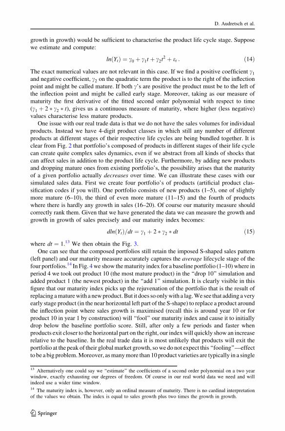
simulated sales data. First we create four portfolio’s of products (artificial product clas-
sification codes if you will). One portfolio consists of new products (1–5), one of slightly
more mature (6–10), the third of even more mature (11–15) and the fourth of products
where there is hardly any growth in sales (16–20). Of course our maturity measure should
correctly rank them. Given that we have generated the data we can measure the growth and
growth in growth of sales precisely and our maturity index becomes:
dlnðYtÞ=dt ¼ c1 þ 2 � c2 � dt ð15Þ
where dt ¼ 1.13 We then obtain the Fig. 3.
One can see that the composed portfolios still retain the imposed S-shaped sales pattern
(left panel) and our maturity measure accurately captures the average lifecycle stage of the
four portfolios.14 In Fig. 4we show thematurity index for a baseline portfolio (1–10)where in
period 4 we took out product 10 (the most mature product) in the ‘‘drop 10’’ simulation and
added product 1 (the newest product) in the ‘‘add 1’’ simulation. It is clearly visible in this
figure that our maturity index picks up the rejuvenation of the portfolio that is the result of
replacing amaturewith a newproduct. But it does so onlywith a lag.We see that adding a very
early stage product (in the near horizontal left part of the S-shape) to replace a product around
the inflection point where sales growth is maximised (recall this is around year 10 or for
product 10 in year 1 by construction) will ‘‘fool’’ our maturity index and cause it to initially
drop below the baseline portfolio score. Still, after only a few periods and faster when
products exit closer to the horizontal part on the right, our indexwill quickly show an increase
relative to the baseline. In the real trade data it is most unlikely that products will exit the
portfolio at the peak of their globalmarket growth, sowe do not expect this ‘‘fooling’’—effect
to be a big problem.Moreover, asmanymore than 10 product varieties are typically in a single
13 Alternatively one could say we ‘‘estimate’’ the coefficients of a second order polynomial on a two yearwindow, exactly exhausting our degrees of freedom. Of course in our real world data we need and willindeed use a wider time window.14 The maturity index is, however, only an ordinal measure of maturity. There is no cardinal interpretationof the values we obtain. The index is equal to sales growth plus two times the growth in growth.
D. Audretsch et al.
123
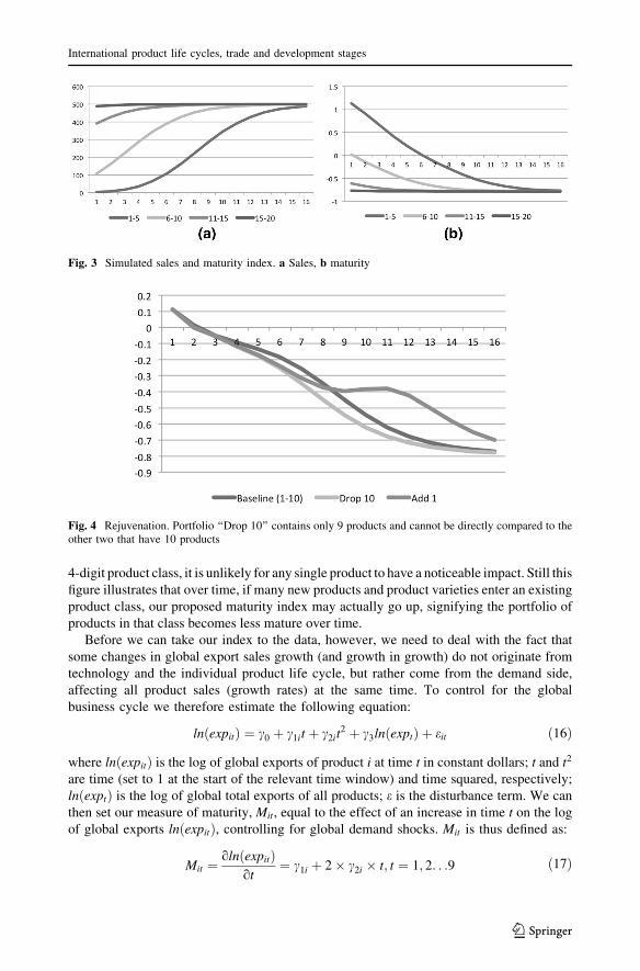
4-digit product class, it is unlikely for any single product to have a noticeable impact. Still this
figure illustrates that over time, if many new products and product varieties enter an existing
product class, our proposed maturity index may actually go up, signifying the portfolio of
products in that class becomes less mature over time.
Before we can take our index to the data, however, we need to deal with the fact that
some changes in global export sales growth (and growth in growth) do not originate from
technology and the individual product life cycle, but rather come from the demand side,
affecting all product sales (growth rates) at the same time. To control for the global
business cycle we therefore estimate the following equation:
lnðexpitÞ ¼ c0 þ c1it þ c2it2 þ c3lnðexptÞ þ eit ð16Þ
where lnðexpitÞ is the log of global exports of product i at time t in constant dollars; t and t2
are time (set to 1 at the start of the relevant time window) and time squared, respectively;
lnðexptÞ is the log of global total exports of all products; e is the disturbance term. We can
then set our measure of maturity, Mit, equal to the effect of an increase in time t on the log
of global exports lnðexpitÞ, controlling for global demand shocks. Mit is thus defined as:
Mit ¼olnðexpitÞ
ot¼ c1i þ 2� c2i � t; t ¼ 1; 2. . .9 ð17Þ
Fig. 3 Simulated sales and maturity index. a Sales, b maturity
Fig. 4 Rejuvenation. Portfolio ‘‘Drop 10’’ contains only 9 products and cannot be directly compared to theother two that have 10 products
International product life cycles, trade and development stages
123
where we have taken a 9 year window to estimate the moments of total global exports.
Assuming the typical S-shaped pattern of sales over the life cycle we can show that the
lower (more negative) Mit is, the more mature a product is. For early stage products both
coefficients are typically positive, whereas for more mature products first c2i and then c1iwill first show up insignificant and than negative in the regression.
We calculated Mit for each of the 427 SITC four-digit products over the period
1988–2005 using global-level export data retrieved from the UN-COMTRADE database.15
More specifically, we estimate Eq. (16) taking a rolling window of 9 years, namely 1988–
1996, 1989–1997, 1990–1998, 1991–1999, 1992–2000, 1993–2001, 1994–2002, 1995–
2003, 1996–2004, 1997–2005 setting the first year to 1 to calculate Mit as in Eq. (17) and
taking the average of all Mit over the different sub-samples. This implies that only if we
estimate different coefficients per window, the corresponding average maturity for that
window will change over time. In this way, we allow for maturity to change over time in a
non-linear fashion and movements up and down are allowed.16
Four important aspects of our measure Mit are worth pointing out at this stage. First, in
contrast to a binary measure to classify industries into either ‘‘growing’’ or ‘‘declining’’ as
in Audretsch (1987), our measure is continuous.17 This property permits a sensible ranking
of products based on maturity level in the global export market.
Second, our measure is time-varying. In other words, we allow products to move from
one stage of the life cycle to the next and back. This latter property may seem undesirable,
but in fact there are good reasons not to exclude such dynamics by construction. As we
have illustrated above, mature product categories can rejuvenate through the upgrading of
existing products and/or the introduction of new product varieties in the same product
category. Such rejuvenation could set off a new S-shaped pattern in global sales that we
want our measure to pick up. In this respect, our measure also differs from Bos et al.
(2013) who evaluates Eq. (17) at the mean of t for all industries and does not allow for the
changes of product maturity over time.
Third, we based our measure on the global exports of a product. Under the assumption
that total global exports correlate with total global production and sales, this will reflect the
true product life cycle. Our proxy, however, will also carry some exogenous elements that
reflect the growth potential of products in the global market place. As we are interested in
the composition of countries’ export bundles, however, it seems only fitting we consider
the global market for classifying products as mature or early stage.
Finally, we prefer a product specific measure based on global export volumes over the
alternative of country level maturity measures as this measure is less prone to endogeneity
15 For the estimation purpose, we keep products that have at least have 5 observations during 18 years. Theaverage number of observations per product is 16. We drop 180 products that are in the residual categories‘‘X’’ since the export data on those products are subject to serious measurement problems. These productsonly account for on average less than 1% of the global export over our sample period.16 We also estimated Eq. (16) using all information 1988–2005, evaluating Mit at each point in timet = 1...18. That, however, is a very rough approximation of our preferred approach, as it makes maturitylinearly dependent on time by construction and does not allow for the estimated slope coefficients to changeover time. The pairwise correlation of the maturity measures computed in these ways is 0.23 (significant at1%), and the Spearman rank-order correlation is 0.38 (where the null hypothesis that both measures areindependent is rejected). This suggests some similarity in their ability to rank products by maturity, butcorrelations are in fact quite low. As the rolling window approach only allows maturity to change over timewhen the estimated coefficients change we chose the rolling window approach as our preferred measure.17 Audretsch (1987) suggests to consider the sign and significance of c1i and c2i to classify industries. Anindustry is classified as growing when either c2i was positive and statistically significant at the 90% level orc2i was statistically insignificant, but c1i was positive and statistically significant.
D. Audretsch et al.
123
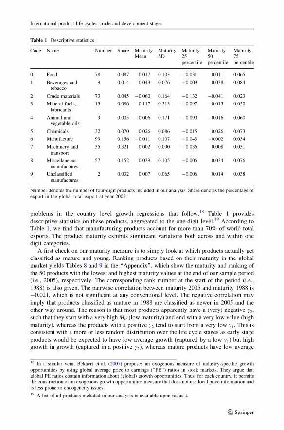
problems in the country level growth regressions that follow.18 Table 1 provides
descriptive statistics on these products, aggregated to the one-digit level.19 According to
Table 1, we find that manufacturing products account for more than 70% of world total
exports. The product maturity exhibits significant variations both across and within one
digit categories.
A first check on our maturity measure is to simply look at which products actually get
classified as mature and young. Ranking products based on their maturity in the global
market yields Tables 8 and 9 in the ‘‘Appendix’’, which show the maturity and ranking of
the 50 products with the lowest and highest maturity values at the end of our sample period
(i.e., 2005), respectively. The corresponding rank number at the start of the period (i.e.,
1988) is also given. The pairwise correlation between maturity 2005 and maturity 1988 is
-0.021, which is not significant at any conventional level. The negative correlation may
imply that products classified as mature in 1988 are classified as newer in 2005 and the
other way around. The reason is that most products apparently have a (very) negative c2,such that they start with a very highMit (low maturity) and end with a very low value (high
maturity), whereas the products with a positive c2 tend to start from a very low c1. This isconsistent with a more or less random distribution over the life cycle stages as early stage
products would be expected to have low average growth (captured by a low c1) but highgrowth in growth (captured in a positive c2), whereas mature products have low average
Table 1 Descriptive statistics
Code Name Number Share Maturity Maturity Maturity Maturity MaturityMean SD 25
percentile50percentile
75percentile
0 Food 78 0.087 0.017 0.103 -0.031 0.011 0.065
1 Beverages andtobacco
9 0.014 0.043 0.076 -0.009 0.038 0.084
2 Crude materials 73 0.045 -0.060 0.164 -0.132 -0.041 0.023
3 Mineral fuels,lubricants
13 0.086 -0.117 0.513 -0.097 -0.015 0.050
4 Animal andvegetable oils
9 0.005 -0.006 0.171 -0.090 -0.016 0.060
5 Chemicals 32 0.070 0.026 0.086 -0.015 0.026 0.073
6 Manufacture 99 0.156 -0.011 0.107 -0.043 -0.002 0.034
7 Machinery andtransport
55 0.321 0.002 0.090 -0.036 0.008 0.051
8 Miscellaneousmanufactures
57 0.152 0.039 0.105 -0.006 0.034 0.076
9 Unclassifiedmanufactures
2 0.032 0.007 0.065 -0.006 0.014 0.038
Number denotes the number of four-digit products included in our analysis. Share denotes the percentage ofexport in the global total export at year 2005
18 In a similar vein, Bekaert et al. (2007) proposes an exogenous measure of industry-specific growthopportunities by using global average price to earnings (‘‘PE’’) ratios in stock markets. They argue thatglobal PE ratios contain information about (global) growth opportunities. Thus, for each country, it permitsthe construction of an exogenous growth opportunities measure that does not use local price information andis less prone to endogeneity issues.19 A list of all products included in our analysis is available upon request.
International product life cycles, trade and development stages
123
growth and negative growth in growth. The Spearman rank correlation (0.053), however,
shows that the ranking at 1988 and 2005 is independent (p value is 0.254).
The products at the extremes of the ranking, are perhaps not making a very convincing
case at first glance. In particular, the list of least mature products includes several raw
materials, ores, basic metals and food products that cannot be considered early stage
products. Our measure is clearly sensitive to the 90s resource boom. Rising demand for
many internationally traded raw materials, ores and energy resources have caused the trade
volumes for those commodities to increase faster than the global trade volume for which
we correct. Consequently, the boom in commodities trade is interpreted by our measure as
a rejuvenation of these commodities, when of course nothing has happened to the product
itself. We will leave these products in for now, exactly because this will bias the esti-
mations against finding the results we are most interested in.20 Of course we have also
excluded these products in robustness tests. The reader should keep in mind, however, that
what we measure as maturity is a rough proxy and measurement error is an issue.
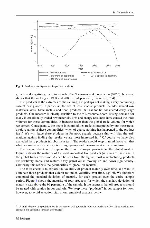
The second check is to explore the trend of major products in the global market.
Figure 5 shows the maturity of the most important five products (in terms of their size in
the global trade) over time. As can be seen from the figure, most manufacturing products
are relatively stable and mature. Only petrol oil is moving up and down significantly.
Obviously this reflects the peculiarities of global oil markets.
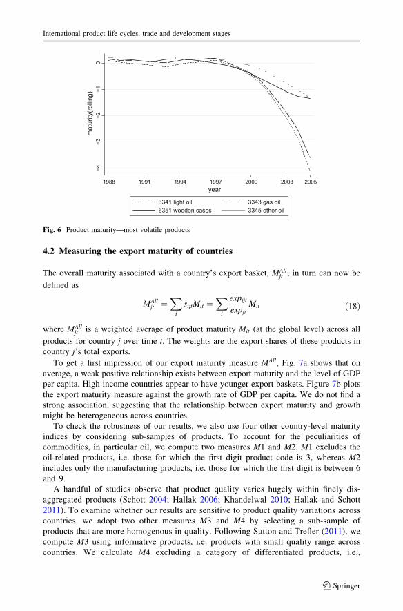
The third check is to explore the volatility of product maturity over time. We want to
eliminate those products that exhibit too much volatility over time, e.g. oil. We therefore
computed the standard deviation of maturity for each product over the entire sample
period. Figure 6 shows the maturity of four products, for which the standard deviation of
maturity was above the 99 percentile of the sample. It too suggests that oil products should
be treated with caution in our analysis. We keep these ‘‘products’’ in our sample for now,
however, to avoid selection bias in our empirical analysis below.
−.4
−.3
−.2
−.1
0.1
mat
urity
(rol
ling)
1988 1991 1994 1997 2000 2003 2005year
lio .lorteP 0333srac rotoM 01877649 Parts of apparatus 9310 Special transaction.7849 Parts of motor vehicle
Fig. 5 Product maturity—most important products
20 A high degree of specialisation in resources will generally bias the positive effect of exporting newproducts on economic growth downwards.
D. Audretsch et al.
123
4.2 Measuring the export maturity of countries
The overall maturity associated with a country’s export basket, MAlljt , in turn can now be
defined as
MAlljt ¼
X
i
sijtMit ¼X
i
expijt
expjtMit ð18Þ
where MAlljt is a weighted average of product maturity Mit (at the global level) across all
products for country j over time t. The weights are the export shares of these products in
country j’s total exports.
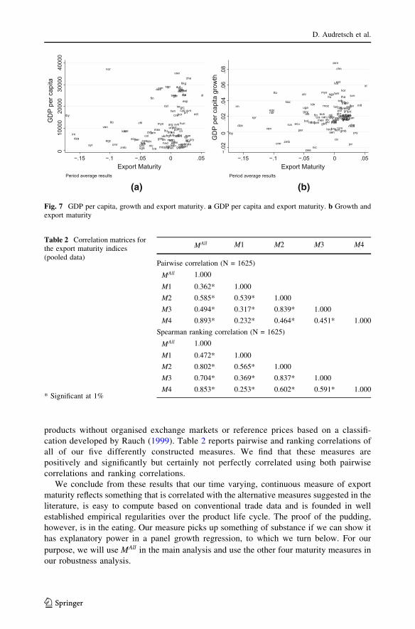
To get a first impression of our export maturity measure MAll, Fig. 7a shows that on
average, a weak positive relationship exists between export maturity and the level of GDP
per capita. High income countries appear to have younger export baskets. Figure 7b plots
the export maturity measure against the growth rate of GDP per capita. We do not find a
strong association, suggesting that the relationship between export maturity and growth
might be heterogeneous across countries.
To check the robustness of our results, we also use four other country-level maturity
indices by considering sub-samples of products. To account for the peculiarities of
commodities, in particular oil, we compute two measures M1 and M2. M1 excludes the
oil-related products, i.e. those for which the first digit product code is 3, whereas M2
includes only the manufacturing products, i.e. those for which the first digit is between 6
and 9.
A handful of studies observe that product quality varies hugely within finely dis-
aggregated products (Schott 2004; Hallak 2006; Khandelwal 2010; Hallak and Schott
2011). To examine whether our results are sensitive to product quality variations across
countries, we adopt two other measures M3 and M4 by selecting a sub-sample of
products that are more homogenous in quality. Following Sutton and Trefler (2011), we
compute M3 using informative products, i.e. products with small quality range across
countries. We calculate M4 excluding a category of differentiated products, i.e.,
−4−3
−2−1
0m
atur
ity(r
ollin
g)
1988 1991 1994 1997 2000 2003 2005year
3341 light oil 3343 gas oil6351 wooden cases 3345 other oil
Fig. 6 Product maturity—most volatile products
International product life cycles, trade and development stages
123
products without organised exchange markets or reference prices based on a classifi-
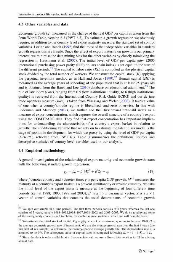
cation developed by Rauch (1999). Table 2 reports pairwise and ranking correlations of
all of our five differently constructed measures. We find that these measures are
positively and significantly but certainly not perfectly correlated using both pairwise
correlations and ranking correlations.
We conclude from these results that our time varying, continuous measure of export
maturity reflects something that is correlated with the alternative measures suggested in the
literature, is easy to compute based on conventional trade data and is founded in well
established empirical regularities over the product life cycle. The proof of the pudding,
however, is in the eating. Our measure picks up something of substance if we can show it
has explanatory power in a panel growth regression, to which we turn below. For our
purpose, we will use MAll in the main analysis and use the other four maturity measures in
our robustness analysis.
alb
arg
arm
ausaut
bel
bgd
bgr
bol
bra
can
che
chl
chncivcmr
colcri
cypcze
deudnk
domdza ecuegy
esp
est
finfragbr
ghagmb
grc
gtm
guy
hkg
hnd
hrv
hun
idnind
irl
irn
isr
ita
jam
jor
jpn
kaz
ken
korlby
lka
ltu lva
marmda
mex
mli
mlt
moz mwi
mys
nic
nld
nor
nzl
pak
panper
phl
pol
prt
pryrom
rus
sen
sgp
slv
svk
svn
swe
syr
tha
tto
tun tur
twn
tzauga
ukr
ury
usa
venzaf
zmb
zwe
010
000
2000
030
000
4000
0G
DP
per
cap
ita
−.15 −.1 −.05 0 .05Export Maturity
Period average results
alb
arg
arm
aus aut belbgdbgrbol
bra
can
che
chl
chn
civcmr
col
cri
cypcze
deudnk
dom
dza ecu
egyesp
est
finfra
gbr
gha
gmb
grc
gtm
guyhkg
hnd
hrv
hun
idn ind
irl
irn
isr itajam
jor
jpn
kaz
ken
kor
lby
lka
ltu
lva
marmda
mexmli
mltmoz
mwi
mys
nic
nldnor
nzl pakpan
per
phl
pol prt
pryrom
rus
sen
sgp
slv
svksvn
swesyr
thatto
tun
tur
twn
tza
uga
ukrury
usa
ven
zaf
zmb
zwe−.02
0.0
2.0
4.0
6.0
8G
DP
per
cap
ita g
row
th
−.15 −.1 −.05 0 .05Export Maturity
Period average results
(a) (b)
Fig. 7 GDP per capita, growth and export maturity. a GDP per capita and export maturity. b Growth andexport maturity
Table 2 Correlation matrices forthe export maturity indices(pooled data)
* Significant at 1%
MAll M1 M2 M3 M4
Pairwise correlation (N = 1625)
MAll 1.000
M1 0.362* 1.000
M2 0.585* 0.539* 1.000
M3 0.494* 0.317* 0.839* 1.000
M4 0.893* 0.232* 0.464* 0.451* 1.000
Spearman ranking correlation (N = 1625)
MAll 1.000
M1 0.472* 1.000
M2 0.802* 0.565* 1.000
M3 0.704* 0.369* 0.837* 1.000
M4 0.853* 0.253* 0.602* 0.591* 1.000
D. Audretsch et al.
123
4.3 Other variables and data
Economic growth (g), measured as the change of the real GDP per capita is taken from the
Penn World Table, version 6.3 (PWT 6.3). To estimate a growth regression we obviously
require, in addition to our country level export maturity measure, the standard set of control
variables. Levine and Renelt (1992) find that most of the independent variables in standard
growth regressions are fragile. Since the effect of export maturity on growth is our primary
interest, we minimise the data mining bias for the other variables by closely mimicking the
regression in Hausmann et al. (2007). The initial level of GDP per capita gdp0 (2005
international purchasing power parity (PPP) dollars chain index) is set equal to the start of
the different periods.21 The capital to labor ratio (KL) is computed as the physical capital
stock divided by the total number of workers. We construct the capital stock (K) applying
the perpetual inventory method as in Hall and Jones (1999).22 Human capital (HC) is
measured as the average years of schooling of the population that is at least 25 years old
and is obtained from the Barro and Lee (2010) database on educational attainment.23 The
rule of law index (Law), ranging from 0.5 (low institutional quality) to 6 (high institutional
quality) is retrieved from the International Country Risk Guide (ICRG) and our de jure
trade openness measure (Jure) is taken from Wacziarg and Welch (2008). It takes a value
of one when a country’s trade regime is liberalised, and zero otherwise. In line with
Lederman and Maloney (2012), we further add the Hirschman-Herfindahl index as a
measure of export concentration, which captures the overall structure of a country’s export
using the COMTRADE data. They find that export concentration has important implica-
tions for understanding the characteristics of a country’s export basket in relation to
growth. The conditioning variable that we rely on to estimate the latent class model is the
stage of economic development for which we proxy by using the level of GDP per capita
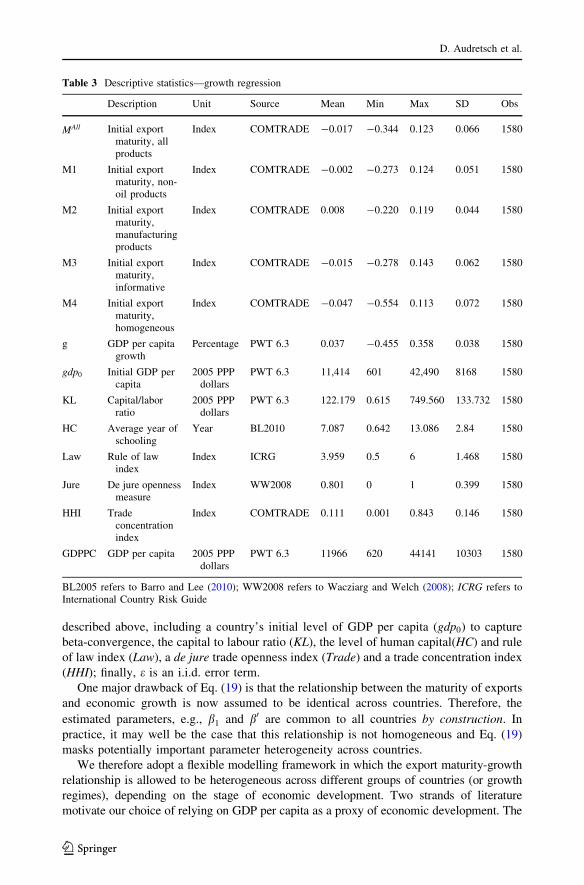
(GDPPC), retrieved from PWT 6.3. Table 3 summarises the definitions, sources and
descriptive statistics of country-level variables used in our analysis.
4.4 Empirical methodology
A general investigation of the relationship of export maturity and economic growth starts
with the following standard growth regression:
gjt ¼ b0 þ b1MAlljt þ b0Zjt þ ejt ð19Þ
where j denotes country and t denotes time; g is per capita GDP growth; MAll measures the
maturity of a country’s export basket; To prevent simultaneity or reverse causality, we take
the initial level of the export maturity measure at the beginning of four different time
periods (i.e., at 1988, 1993, 1998 and 2003); b0 is a 1� n parameter vector; Z is a n� 1
vector of control variables that contains the usual determinants of economic growth
21 We split our sample in 4 time periods. The first three periods consists of 5 years, whereas the last oneconsists of 3 years, namely 1988–1992,1993–1997,1998–2002 and 2003–2005. We do so to alleviate someof the endogeneity concerns and to obtain reasonable regime switches, which we will describe later.
22 We estimate the initial stock of capital, Kt0 asIt0Gþd, where I is investment, t0 refers to the year 1988, G is
the average geometric growth rate of investment. We use the average growth rate over the first 9 years (thefirst half of our sample) to determine the country-specific average growth rate. The depreciation rate d isassumed to be 6%. The subsequent value of capital stock is computed following Kt ¼ ð1� dÞKt�1 þ It.23 Since the data is only available at a five-year interval, we use a linear interpolation to fill in missingannual data.
International product life cycles, trade and development stages
123
described above, including a country’s initial level of GDP per capita (gdp0) to capture
beta-convergence, the capital to labour ratio (KL), the level of human capital(HC) and rule
of law index (Law), a de jure trade openness index (Trade) and a trade concentration index
(HHI); finally, e is an i.i.d. error term.
One major drawback of Eq. (19) is that the relationship between the maturity of exports
and economic growth is now assumed to be identical across countries. Therefore, the
estimated parameters, e.g., b1 and b0 are common to all countries by construction. In
practice, it may well be the case that this relationship is not homogeneous and Eq. (19)
masks potentially important parameter heterogeneity across countries.
We therefore adopt a flexible modelling framework in which the export maturity-growth
relationship is allowed to be heterogeneous across different groups of countries (or growth
regimes), depending on the stage of economic development. Two strands of literature
motivate our choice of relying on GDP per capita as a proxy of economic development. The
Table 3 Descriptive statistics—growth regression
Description Unit Source Mean Min Max SD Obs
MAll Initial exportmaturity, allproducts
Index COMTRADE -0.017 -0.344 0.123 0.066 1580
M1 Initial exportmaturity, non-oil products
Index COMTRADE -0.002 -0.273 0.124 0.051 1580
M2 Initial exportmaturity,manufacturingproducts
Index COMTRADE 0.008 -0.220 0.119 0.044 1580
M3 Initial exportmaturity,informative
Index COMTRADE -0.015 -0.278 0.143 0.062 1580
M4 Initial exportmaturity,homogeneous
Index COMTRADE -0.047 -0.554 0.113 0.072 1580
g GDP per capitagrowth
Percentage PWT 6.3 0.037 -0.455 0.358 0.038 1580
gdp0 Initial GDP percapita
2005 PPPdollars
PWT 6.3 11,414 601 42,490 8168 1580
KL Capital/laborratio
2005 PPPdollars
PWT 6.3 122.179 0.615 749.560 133.732 1580
HC Average year ofschooling
Year BL2010 7.087 0.642 13.086 2.84 1580
Law Rule of lawindex
Index ICRG 3.959 0.5 6 1.468 1580
Jure De jure opennessmeasure
Index WW2008 0.801 0 1 0.399 1580
HHI Tradeconcentrationindex
Index COMTRADE 0.111 0.001 0.843 0.146 1580
GDPPC GDP per capita 2005 PPPdollars
PWT 6.3 11966 620 44141 10303 1580
BL2005 refers to Barro and Lee (2010); WW2008 refers to Wacziarg and Welch (2008); ICRG refers toInternational Country Risk Guide
D. Audretsch et al.
123
first strand has examined the heterogeneity of growth experience of countries in general and
has well established the substantial differences in the determinants of growth between
developing and developed countries. These studies (e.g., Durlauf and Johnson 1995; Canova
2004; Papageorgiou 2002) typically use the initial level of GDP per capita as a regime
splitting variable to examine multiple growth regimes. However, such an ex ante classifi-
cation is somewhat arbitrary and subject to debate since the appropriate cut-off point is not
always clear. In contrast, our approach endogenizes the cut-off points and is thus much more
flexible. The second strand has established a non-linear relationship between export structure
(specialised vs. diversified) and economic growth (Imbs and Wacziarg 2003; Aditya and Roy
2007; Cadot et al. 2007; Hesse 2008). These papers typically find that the relationship differs
by the development stage of countries as proxied by GDP per capita.
We thus treat the stage of development as a latent variable, and use a latent class model to
endogenise the sorting of countries into different growth regimes. To model the latent vari-
able, we use a multinomial logit sorting equation, and include the stage of development,
proxied by real GDP per capita, to estimate the likelihood of being in a particular growth
regime. Our conditional latent class model consists of a system of two equations: an equation
to estimate the maturity-growth nexus for each regime, and a multinomial sorting equation
where the regime membership is a function of the development stage, i.e. GDP per capita.
To allow for endogenous sorting into regimes kð¼ 1; . . .KÞ, we can rewrite Eq. (19) as
follows:
gjtjk ¼ bk þ b1jkMAlljt þ b0kZjt þ ejtjk ð20Þ
where k ¼ 1; . . .;K indicates the regime and K refers to the (endogenous) total number of
regimes. Each regime has its own parameter vector b. In other words, b0, b1, b0 are allowed
to differ across regimes.
To estimate Eq. (20), we must first find the suitable number of K. As this is not a
parameter to be estimated directly from Eq. (20) Greene (2007) suggests a ‘‘test-down’’
strategy to identify the correct number of regimes. A specification with K þ 1 regimes is
inferior to one with K regimes if the parameters in any two of the K þ 1 classes are equal
(statistically indistinguishable). If the true K is unknown, it is possible to test down from
K þ n to K using a log likelihood ratio test.24
Our aim is then to sort each observation jt into a discrete regime k. This is done by
specifying the contribution of each observation jt to the likelihood function, conditional on
its regime membership. The unconditional likelihood for each observation jt is obtained as
a weighted average of its regime-specific likelihood using the prior probability of being in
regime k as weights. Since we do not observe directly which regime will contain a par-
ticular observation jt, the group membership probability hjt must be estimated. In our
conditional latent class framework, we make this probability conditional on GDP per capita
(GDPPC) and parameterise hjt by means of a multinomial logit model:
hjt ¼expðGDPPCjthkÞPKk¼1 expðGDPPCjthkÞ
ð21Þ
where hjt measures the odds of being in regime k, conditional on GDPPC. The likelihood
for the entire sample, which is the sum of all unconditional likelihood over all jt resulting
24 Theoretically, the maximum number of regimes is only restricted by the number of cross-sections, i.e. thenumber of observations in the data. However, empirically the overspecification problem limits the esti-mation of a large number of regimes.
International product life cycles, trade and development stages
123
from Eqs. (20) and (21), can then be maximised with respect to the parameter vector
b ¼ ðb1; . . .bKÞ and the latent class parameter vector h ¼ ðh1; . . .hKÞ; hK ¼ 0 using a
conventional maximum likelihood estimator, following Greene (2007). With the parameter
vector b and h in hand, a posterior estimate of the regime membership probability for each
observation jt, can be computed using Bayes’ theorem. Each observation can then be
assigned to the regime with the largest posterior probability.
One distinctive feature of our approach is that we allow countries to switch between
regimes over time, following e.g. Bos et al. (2010). We do want to avoid countries close to
a switching point, however, from switching back and forth between regimes all the time.
We therefore split our sample in four time periods and allow countries to only switch
regimes between these four periods. Essentially we pooled together the observations from
the time periods and treated observations within these periods as independent draws from
the same regime. This implies that one country can be allocated to one particular regime
k in period 1 (1988–1992) and another one in period 2 (1993–1997), but no switches occur
within these periods by construction. This adds flexibility into our modelling framework by
avoiding the imposed assumption of persistent regime allocation and provides additional
insights into regime switches. We can thus study the dynamics of the maturity-growth
relationship as countries move along their development path at different speeds.
To summarise our empirical strategy, we employ a conditional latent class model to
examine for the possible non-linear relationship between export maturity and growth in
K endogenously determined regimes. The regime membership probabilities are conditional
on the stage of economic development.
5 Empirical results
5.1 Main results
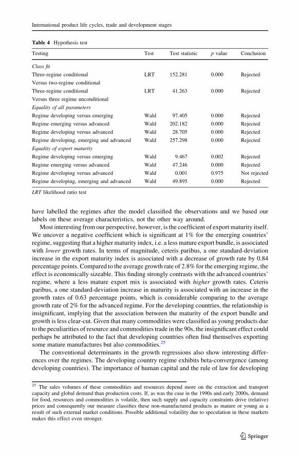
Wefirst determine the number of regimes in our data following the suggestion byGreene (2007).
The test results in the top row in Table 4 favour a specification with three regimes over the one
with two regimes. We refer to these regimes as developing, emerging and advanced for reasons
we will explain later. Moreover, the second row shows that the unconditional latent class model
must be rejected in favour of the conditional one. Next, we test whether the parameter estimates
differ significantly across regimes by means ofWald tests for joint equality. The results indicate
that the equality of all parameters should be rejected at the 1% significance level across regimes.
Finally, we test whether the effect of export maturity on growth is significantly different across
regimes. The Wald tests here reveal that the effects are jointly significantly different across the
three regimes, except between the developing and advanced regime.
From this table we conclude that a three regime, conditional latent class specification is
most suitable for our purpose. Then we turn to the effect of the maturity of a country’s
export portfolio on economic growth across these regimes by looking at the conditional
latent class estimation results in Table 5.
First observe in the lower part of the table that the first regime has a low average GDP
per capita, the most mature export bundle and the lowest average growth rate. We therefore
labeled this regime ‘‘developing’’. The second ‘‘emerging’’ regime has still low but slightly
higher average levels of GDP per capita, a considerably higher average growth rate and an
intermediate average maturity. The ‘‘advanced’’ regime has a high average level of GDP
per capita, moderate growth rates and the lowest average maturity of exports. Note that we
D. Audretsch et al.
123
have labelled the regimes after the model classified the observations and we based our
labels on these average characteristics, not the other way around.
Most interesting from our perspective, however, is the coefficient of export maturity itself.
We uncover a negative coefficient which is significant at 1% for the emerging countries’
regime, suggesting that a higher maturity index, i.e. a less mature export bundle, is associated
with lower growth rates. In terms of magnitude, ceteris paribus, a one standard-deviation
increase in the export maturity index is associated with a decrease of growth rate by 0.84
percentage points. Compared to the average growth rate of 2.8% for the emerging regime, the
effect is economically sizeable. This finding strongly contrasts with the advanced countries’
regime, where a less mature export mix is associated with higher growth rates. Ceteris
paribus, a one standard-deviation increase in maturity is associated with an increase in the
growth rates of 0.63 percentage points, which is considerable comparing to the average
growth rate of 2% for the advanced regime. For the developing countries, the relationship is
insignificant, implying that the association between the maturity of the export bundle and
growth is less clear-cut. Given that many commodities were classified as young products due
to the peculiarities of resource and commodities trade in the 90s, the insignificant effect could
perhaps be attributed to the fact that developing countries often find themselves exporting
some mature manufactures but also commodities.25
The conventional determinants in the growth regressions also show interesting differ-
ences over the regimes. The developing country regime exhibits beta-convergence (among
developing countries). The importance of human capital and the rule of law for developing
Table 4 Hypothesis test
Testing Test Test statistic p value Conclusion
Class fit
Three-regime conditional LRT 152.281 0.000 Rejected
Versus two-regime conditional
Three-regime conditional LRT 41.263 0.000 Rejected
Versus three regime unconditional
Equality of all parameters
Regime developing versus emerging Wald 97.405 0.000 Rejected
Regime emerging versus advanced Wald 202.182 0.000 Rejected
Regime developing versus advanced Wald 28.705 0.000 Rejected
Regime developing, emerging and advanced Wald 257.298 0.000 Rejected
Equality of export maturity
Regime developing versus emerging Wald 9.467 0.002 Rejected
Regime emerging versus advanced Wald 47.246 0.000 Rejected
Regime developing versus advanced Wald 0.001 0.975 Not rejected
Regime developing, emerging and advanced Wald 49.895 0.000 Rejected
LRT likelihood ratio test
25 The sales volumes of these commodities and resources depend more on the extraction and transportcapacity and global demand than production costs. If, as was the case in the 1990s and early 2000s, demandfor food, resources and commodities is volatile, then such supply and capacity constraints drive (relative)prices and consequently our measure classifies these non-manufactured products as mature or young as aresult of such external market conditions. Possible additional volatility due to speculation in these marketsmakes this effect even stronger.
International product life cycles, trade and development stages
123
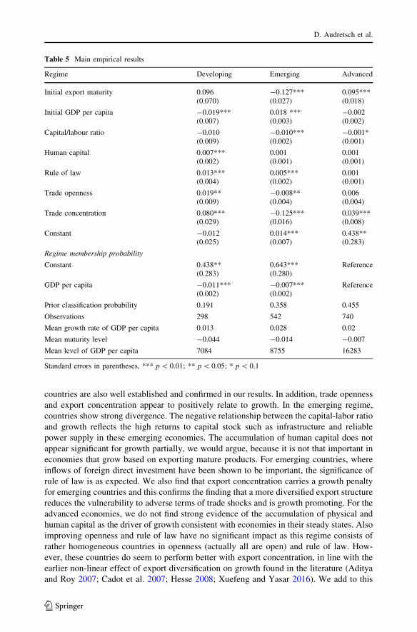
countries are also well established and confirmed in our results. In addition, trade openness
and export concentration appear to positively relate to growth. In the emerging regime,
countries show strong divergence. The negative relationship between the capital-labor ratio
and growth reflects the high returns to capital stock such as infrastructure and reliable
power supply in these emerging economies. The accumulation of human capital does not
appear significant for growth partially, we would argue, because it is not that important in
economies that grow based on exporting mature products. For emerging countries, where
inflows of foreign direct investment have been shown to be important, the significance of
rule of law is as expected. We also find that export concentration carries a growth penalty
for emerging countries and this confirms the finding that a more diversified export structure
reduces the vulnerability to adverse terms of trade shocks and is growth promoting. For the
advanced economies, we do not find strong evidence of the accumulation of physical and
human capital as the driver of growth consistent with economies in their steady states. Also
improving openness and rule of law have no significant impact as this regime consists of
rather homogeneous countries in openness (actually all are open) and rule of law. How-
ever, these countries do seem to perform better with export concentration, in line with the
earlier non-linear effect of export diversification on growth found in the literature (Aditya
and Roy 2007; Cadot et al. 2007; Hesse 2008; Xuefeng and Yasar 2016). We add to this
Table 5 Main empirical results
Regime Developing Emerging Advanced
Initial export maturity 0.096(0.070)
-0.127***(0.027)
0.095***(0.018)
Initial GDP per capita -0.019***(0.007)
0.018 ***(0.003)
-0.002(0.002)
Capital/labour ratio -0.010(0.009)
-0.010***(0.002)
-0.001*(0.001)
Human capital 0.007***(0.002)
0.001(0.001)
0.001(0.001)
Rule of law 0.013***(0.004)
0.005***(0.002)
0.001(0.001)
Trade openness 0.019**(0.009)
-0.008**(0.004)
0.006(0.004)
Trade concentration 0.080***(0.029)
-0.125***(0.016)
0.039***(0.008)
Constant -0.012(0.025)
0.014***(0.007)
0.438**(0.283)
Regime membership probability
Constant 0.438**(0.283)
0.643***(0.280)
Reference
GDP per capita -0.011***(0.002)
-0.007***(0.002)
Reference
Prior classification probability 0.191 0.358 0.455
Observations 298 542 740
Mean growth rate of GDP per capita 0.013 0.028 0.02
Mean maturity level -0.044 -0.014 -0.007
Mean level of GDP per capita 7084 8755 16283
Standard errors in parentheses, *** p\ 0.01; ** p\ 0.05; * p\ 0.1
D. Audretsch et al.
123
literature by showing that diversifying exports into a wider range of mature products is
probably most effective and relevant for developing and emerging countries, whereas
concentrating exports on a range of new products has a positive connection to growth for
advanced countries.
There are three reasons why we conclude that our latent class specification does not
merely sort country-time observations in such a way that these results endogenously
emerge. First, the significantly negative coefficient on GDP per capita in the regime
membership probability estimation signifies that lower GDP per capita increases the
probability of moving from the reference group to the emerging and developing regimes,
respectively, where the latter effect is stronger. This implies that countries with high GDP
per capita tend to be sorted into the advanced regime, whereas countries with medium GDP
per capita sort into the emerging regime and low income countries end up in the devel-
oping regime.26 In an unconditional latent class specification the three regimes might
simply emerge because the model fits the data better if one sorts the observations for which
a negative, positive and indeterminate effect applies. The fact that GDP per capita has
predictive power in the sorting suggests, however, that there is more to these regimes.
Second, in Table 6 we present the regime classifications over time for selected coun-
tries. It can be verified that most of the G7 countries are in the advanced growth regime,
most of the time, with an occasional switch to the emerging regime and back. The newly
industrialised countries in South East Asia, South Africa and Brazil are classified in most
periods into the emerging regime and occasionally move between the developing and
emerging regimes (with the exception of Singapore which moves from the advanced to
developing regime. Financial services, re-exports and port logistics may well have driven
this outlier).27 Interestingly, the exports of mature products by China may constitute an
important factor to explain the recent rapid growth and strong convergence of the newly
industrialised countries. Our classification is not completely in line with our priors (e.g.,
Japan classified as emerging in 1988–1992 or Brazil as advanced since 1998), but on the
whole the classification looks roughly fine, considering that this classification is in no way
based on ex ante assumptions and exogenous thresholds or cut-off points.
A final distinctive feature of ourmodel is that a countrymay change regimes over time. Thus,
we can examine the stability of the regime classification by considering regime switches over
time. Table 7 presents the regime transition matrix, including the absolute number of regime
allocation changes and the frequency between any two time periods.28 We can see that the
diagonal elements carry the largest percentages, as would be expected. However, there are quite
some transitions fromemerging toadvancedandback.Transitionsbetween the advancedand the
developing regime are more rare, as is to be expected. Transitions from developing to emerging
and back aremuchmore frequent than between developing and advanced. The emerging regime
thus seems to be the stepping stone towards the advanced country growth regime.
The occasional switches from developing to advanced and back can also be due, in part, to
the disrupting effects of resource and commodities trading, as was argued above. This,
however, requires much more detailed analysis of the transition dynamics in our data. A
useful first step in that direction would be to redo our analysis without products that can be
classified as primary sector products. We feel, however, that at this stage it is useful to leave
26 Of course we have named these regimes accordingly ex post and based on this outcome. The modelendogenously identifies three statistically distinct classes/growth regimes.27 The full classification of countries in growth regimes is presented in Table 10 in the ‘‘Appendix’’.28 Since we distinguish four time periods, we have three transition matrices. We opt to present theaggregate, unconditional transition probabilities, following Bos et al. (2010).
International product life cycles, trade and development stages
123
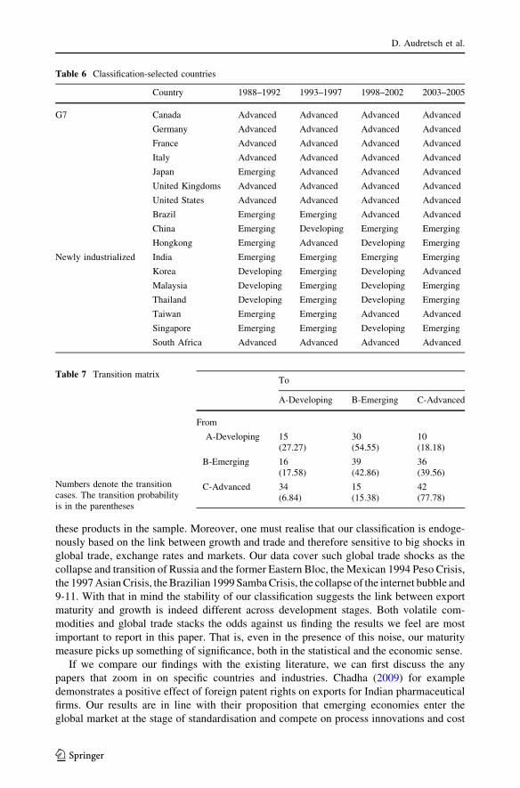
these products in the sample. Moreover, one must realise that our classification is endoge-
nously based on the link between growth and trade and therefore sensitive to big shocks in
global trade, exchange rates and markets. Our data cover such global trade shocks as the
collapse and transition of Russia and the former Eastern Bloc, the Mexican 1994 Peso Crisis,
the 1997AsianCrisis, theBrazilian 1999SambaCrisis, the collapse of the internet bubble and
9-11. With that in mind the stability of our classification suggests the link between export
maturity and growth is indeed different across development stages. Both volatile com-
modities and global trade stacks the odds against us finding the results we feel are most
important to report in this paper. That is, even in the presence of this noise, our maturity
measure picks up something of significance, both in the statistical and the economic sense.
If we compare our findings with the existing literature, we can first discuss the any
papers that zoom in on specific countries and industries. Chadha (2009) for example
demonstrates a positive effect of foreign patent rights on exports for Indian pharmaceutical
firms. Our results are in line with their proposition that emerging economies enter the
global market at the stage of standardisation and compete on process innovations and cost
Table 6 Classification-selected countries
Country 1988–1992 1993–1997 1998–2002 2003–2005
G7 Canada Advanced Advanced Advanced Advanced
Germany Advanced Advanced Advanced Advanced
France Advanced Advanced Advanced Advanced
Italy Advanced Advanced Advanced Advanced
Japan Emerging Advanced Advanced Advanced
United Kingdoms Advanced Advanced Advanced Advanced
United States Advanced Advanced Advanced Advanced
Brazil Emerging Emerging Advanced Advanced
China Emerging Developing Emerging Emerging
Hongkong Emerging Advanced Developing Emerging
Newly industrialized India Emerging Emerging Emerging Emerging
Korea Developing Emerging Developing Advanced
Malaysia Developing Emerging Developing Emerging
Thailand Developing Emerging Developing Emerging
Taiwan Emerging Emerging Advanced Advanced
Singapore Emerging Emerging Developing Emerging
South Africa Advanced Advanced Advanced Advanced
Table 7 Transition matrix
Numbers denote the transitioncases. The transition probabilityis in the parentheses
To
A-Developing B-Emerging C-Advanced
From
A-Developing 15(27.27)
30(54.55)
10(18.18)
B-Emerging 16(17.58)
39(42.86)
36(39.56)
C-Advanced 34(6.84)
15(15.38)
42(77.78)
D. Audretsch et al.
123
advantages, but different in a way that we do not specify the source of cost advantages for
the emerging economies, which Chadha (2009) argues could arise from labor, capital or
technology. A large number of studies have documented extensively the economic success
and industrial achievements of the East Asian economies and an interesting strand of
literature takes a closer look at the strategies of the firms in these economies (Hobday
1995; Hobday et al. 2004; Choung et al. 2014). In particular, they show that companies in
these countries are showing a strong tendency to go beyond exploiting existing technology
and competing on mature markets, rather they compete as frontier players with new and
innovative products in the global market.29 They provide evidence that firms progressed
from learning the techniques of manufacturing processes (e.g. strategic partnership, inte-
gration in global value chain) and developing competences to eventually engaging in R&D
and introducing young and innovative products (Hobday et al. 2004; Pietrobelli and
Rabellotti 2011; Choung et al. 2014). Our results corroborate these findings in the litera-
ture that emerging economies tend to perform better by exporting mature products but face
the challenge of making a transition from copying mature to inventing new products and
joining the advanced economies at the frontier. However, these studies do not measure the
maturity of the product market directly, nor do they examine the implications of such
effects found for the advanced economies. Our paper fills this gap by introducing a novel,
macro level measure of product maturity, and assessing the effect of export maturity on
country performance instead. With our measure we are thus able to study the relationship
between export maturity and growth across a number of countries.
Our results extend and complement recent studies that examine the linkages between the
product characteristics of exports and economic growth (Feenstra and Rose 2000; Bensidoun
et al. 2002; An and Iyigun 2004; Hausmann et al. 2007; Lee 2011). Table 5 not only shows that
exportmaturity aswehavemeasured it,matters for growth. It also shows that this effect depends
on the stage of economic development and is significantly non-linear in the level of GDP per
capita. This finding is contrary to the common conclusion that emerges from the literature. In
spite of a wide variety of measures, specifications and econometric techniques used, it typically
postulates a linear monotonic relationship between specific characteristics of exports and
growth. Consistent with the notion that ‘‘what you export matters’’, however, our findings
suggest that the timing of exports in relation to the development process matters as well.
5.2 Robustness analyses
We conducted several robustness checks that show that our results are insensitive to the
choice of particular maturity measures. First, to account for the peculiarities of com-
modities, in particular oil, we consider two alternative export maturity measures: M1 that
excludes the oil-related products, and M2, which only includes manufacturing products.
We report the specification test results in Tables 11 and 12 in the ‘‘Appendix’’, respec-
tively. Again, these statistical tests indicate that a three-regime conditional latent class
model is preferable. The estimation results are shown in Tables 13 and 14 in the ‘‘Ap-
pendix’’, respectively. The non-linear relationship between export maturity and growth
over three development stages is found to be rather similar to those reported in Table 5. We
observe a significant positive relationship between a higher maturity index and growth for
29 Hobday et al. (2004) find that electronic firms in the East Asian countries export a portfolio of productsthat consists of both low- and high-tech products. This evidence suggest that firms may simultaneouslypursue a mixture of imitation-based growth and innovation-based growth as they go through the cycle ofcatching up and make the transition from latecomer to leader.
International product life cycles, trade and development stages
123
the advanced countries’ regime and a significant negative one for the emerging countries’
regime, albeit the magnitudes are somewhat smaller.
Second, to examine the role of product quality in driving the relationship between
maturity and growth, we use two other measures M3 and M4, following Sutton and Trefler
(2011) and Rauch (1999), respectively. Sutton and Trefler (2011) develop a model pos-
tulating that a country’s wealth and its export mix are simultaneously determined by its
capabilities. Thus, economic growth can be achieved either through the shift to a different
mix of products or through the improvement in quality/productivity in the existing port-
folio of products. Empirically, they demonstrate that the quality range is huge, raising
some concerns about the the informativeness of Hausmann et al. (2007)’s measure. As a
consequence, they illustrate that changes in the export mix may substantially over-predict
economic growth for low-income countries. To define which product is informative, they
plot the GDP per capital of the richest exporter against the GDP per capita of the poorest
exporter for each product in Fig. 8 in the ‘‘Appendix’’. Products that lie in the upper right
or bottom left part of the figure, i.e. those with small quality range are considered infor-
mative.30 As can be seen, informative products constitute a small proportion of total
products. Based on this definition, we identify 191 informative products (out of 430 in our
sample) and calculate M3 using the maturity of these 191 products. Next, we use a
classification developed by Rauch (1999) who distinguish products into homogeneous,
differentiated and an intermediate categories and calculate M4 by dropping the category of
differentiated products. Essentially bothM3 andM4 consider a sub-sample of products that
are more homogenous in quality, are therefore less prone to quality variations across
countries. We expect that the estimated non-linear relationship between maturity and
growth to be stronger when using M3 and M4. The specification tests are shown in
Tables 15 and 16 in the ‘‘Appendix’’, respectively. A conditional three-regime latent class
model is preferred. The estimation results are presented in Tables 17 and 18, respectively.
The results consistently show that the three-regime specification is a very robust feature of
our data. The export maturity measure enters with a positive and statistically significant
coefficient in the advanced countries’ regime, whereas it appears to be significantly neg-
ative in the emerging countries’ regime. The magnitude is considerably larger for the
advanced countries, especially using the maturity measure of informative products M3, but
it is comparable to that found for emerging countries in Table 5.
Overall, our results therefore donot seem tobedrivenby the inclusionof commodities in our
sample or the product quality variations.Arguably, the endogeneity of exportmaturity alsodoes
not pose a serious problem in our analysis for three reasons. First, since we constructed our
product-specificmaturitymeasure using the global data, it is less prone to the endogeneity issue
than using country-level data. This approach captures some exogenous product characteristics
and does not rely on the product information at the country level. Second, we use lagged export
maturity, defined as the level at the beginning of each four periods (i.e. 1988, 1993, 1998, 2003)
in our estimations, to alleviate the reverse causality problem.And third, the identification of the
negative coefficient between export maturity and growth in the emerging regime suggests that
reverse causality cannot be an issue. As countries enjoying higher growth are less likely to
export mature products that are in the declining stage, we feel that the causality running from
export maturity to growth is far more plausible. Therefore we feel confident that the empirical
set-upwe adopted ensures the validity of our estimation results.We now turn to our conclusions
to discuss the significance of our findings.
30 More precisely, the (ln) minimum GDP per capita of the country that produces this good is smaller than8.26 and the (ln) maximum GDP per capita is 9.99.
D. Audretsch et al.
123
6 Conclusions
In this paper, we set out to develop a new measure of product maturity using old knowledge
about the product life cycle. A typical product will diffuse in global trade (if at all) approx-
imately following an S-shaped diffusion curve, where total market volume increases fast,
than slower and eventually goes into decline. In global markets a product was thus defined as
mature when export growth declines. Using this empirical regularity of the product life cycle
we developed a continuous maturity measure and showed that our classification of four-digit
products in global trade is positively correlated but certainly not equivalent to other classi-
ficationmethods in the literature. As our empirical analysis went on to show, our measure has
something sensible and novel to say about countries’ growth performance.
We showed in a conditional latent class growth estimation that countries can find
themselves in three distinct growth regimes. That is, the vector of parameters differs
significantly between three endogenously determined groups of country-time observations
in our data set. In addition, we showed that GDP per capita, as a proxy for the level of
development of a country, is a good predictor of class membership and our model dis-
tinguishes between low, middle and high income level countries. This too is quite similar
to classifications used in the literature, but our classification has the added benefit that we
do not impose group membership or have to rely on inherently arbitrary cut-off points.
Finally, we showed that our export maturity measure has a non-linear impact on eco-
nomic growth over the development stages our countries find themselves in. In the low-
income developing stage the maturity of exports is not significantly related to growth and
such traditional variables as capital-labor ratio’s and that institutional quality picks up most
of the cross-country, within period variation. This implies that for developing countries
getting into or out of mature export products is not expected to affect their growth per-
formance in a predictable direction. In part, this may be due to the fact that some resources
and commodities were classified as early stage products as a result of the late 1990s
resource boom. This would offset the otherwise positive (or negative) impact of manu-
factured early stage products, but we feel it is more likely we would have found a sig-
nificant coefficient in either direction if such biases had been strong. For slightly richer
emerging countries, in contrast, we found a robust and clearly negative relationship
between exporting early stage products and growth. They do better exporting mature
(manufactured) products and moving into large but globally saturated or declining markets.
This gives them the opportunity to grow fast, capturing market share of others. But, in the
advanced country stage, the sign switches and exporting mature products becomes a drag
on growth. The challenge here is clearly to grow fast on mature products but simultane-
ously preparing for the next stage, in which early stage innovative exports take over as the
engine of growth.
This is clearly a huge policy challenge. The existence of distinct growth regimes and
sign-switches between them imply that policies aimed to support the penetration of mature
markets (e.g. lax intellectual property standards, autocratic control over infrastructures,
export subsidies and cheap bank credit) promote growth first, but may put a drag on it in
the next stage of development. The advanced industrialised countries are currently still
making their transition from an industrial, managed society to an entrepreneurial society
(Audretsch and Sanders 2007). The challenge for emerging countries like China, India and
Brazil is to design policies that are flexible enough to take the country to the next stage of
development and then keep it at the frontier. What policies will pass that test is an
empirical matter and left for further research.
International product life cycles, trade and development stages
123
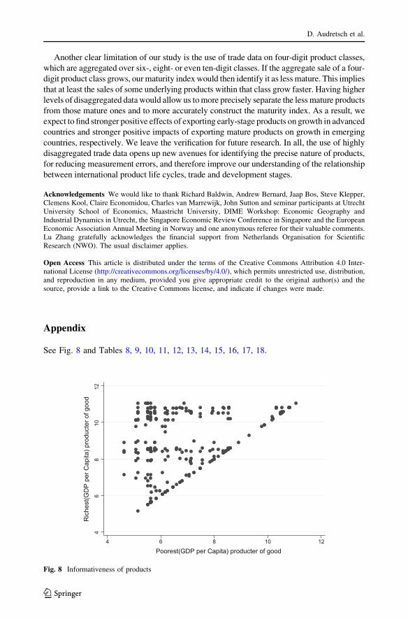
Another clear limitation of our study is the use of trade data on four-digit product classes,
which are aggregated over six-, eight- or even ten-digit classes. If the aggregate sale of a four-
digit product class grows, ourmaturity indexwould then identify it as lessmature. This implies
that at least the sales of some underlying products within that class grow faster. Having higher
levels of disaggregated datawould allow us tomore precisely separate the less mature products
from those mature ones and to more accurately construct the maturity index. As a result, we
expect to find stronger positive effects of exporting early-stage products on growth in advanced
countries and stronger positive impacts of exporting mature products on growth in emerging
countries, respectively. We leave the verification for future research. In all, the use of highly
disaggregated trade data opens up new avenues for identifying the precise nature of products,
for reducing measurement errors, and therefore improve our understanding of the relationship
between international product life cycles, trade and development stages.
Acknowledgements We would like to thank Richard Baldwin, Andrew Bernard, Jaap Bos, Steve Klepper,Clemens Kool, Claire Economidou, Charles van Marrewijk, John Sutton and seminar participants at UtrechtUniversity School of Economics, Maastricht University, DIME Workshop: Economic Geography andIndustrial Dynamics in Utrecht, the Singapore Economic Review Conference in Singapore and the EuropeanEconomic Association Annual Meeting in Norway and one anonymous referee for their valuable comments.Lu Zhang gratefully acknowledges the financial support from Netherlands Organisation for ScientificResearch (NWO). The usual disclaimer applies.
Open Access This article is distributed under the terms of the Creative Commons Attribution 4.0 Inter-national License (http://creativecommons.org/licenses/by/4.0/), which permits unrestricted use, distribution,and reproduction in any medium, provided you give appropriate credit to the original author(s) and thesource, provide a link to the Creative Commons license, and indicate if changes were made.
Appendix
See Fig. 8 and Tables 8, 9, 10, 11, 12, 13, 14, 15, 16, 17, 18.
46
810
12
Ric
hest
(GD
P p
er C
apita
) pro
duct
er o
f goo
d
4 6 8 10 12
Poorest(GDP per Capita) producter of good
Fig. 8 Informativeness of products
D. Audretsch et al.
123
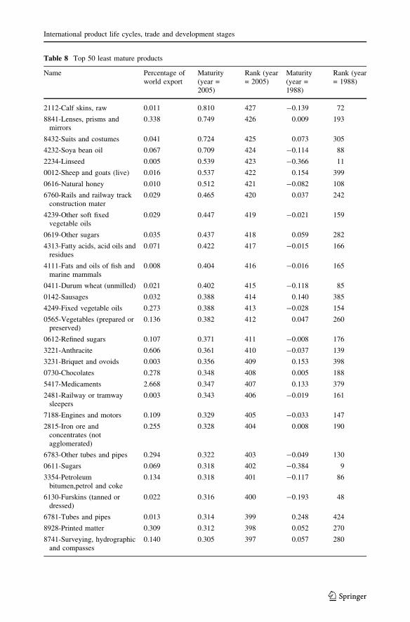
Table 8 Top 50 least mature products
Name Percentage ofworld export
Maturity(year =2005)
Rank (year= 2005)
Maturity(year =1988)
Rank (year= 1988)
2112-Calf skins, raw 0.011 0.810 427 -0.139 72
8841-Lenses, prisms andmirrors
0.338 0.749 426 0.009 193
8432-Suits and costumes 0.041 0.724 425 0.073 305
4232-Soya bean oil 0.067 0.709 424 -0.114 88
2234-Linseed 0.005 0.539 423 -0.366 11
0012-Sheep and goats (live) 0.016 0.537 422 0.154 399
0616-Natural honey 0.010 0.512 421 -0.082 108
6760-Rails and railway trackconstruction mater
0.029 0.465 420 0.037 242
4239-Other soft fixedvegetable oils
0.029 0.447 419 -0.021 159
0619-Other sugars 0.035 0.437 418 0.059 282
4313-Fatty acids, acid oils andresidues
0.071 0.422 417 -0.015 166
4111-Fats and oils of fish andmarine mammals
0.008 0.404 416 -0.016 165
0411-Durum wheat (unmilled) 0.021 0.402 415 -0.118 85
0142-Sausages 0.032 0.388 414 0.140 385
4249-Fixed vegetable oils 0.273 0.388 413 -0.028 154
0565-Vegetables (prepared orpreserved)
0.136 0.382 412 0.047 260
0612-Refined sugars 0.107 0.371 411 -0.008 176
3221-Anthracite 0.606 0.361 410 -0.037 139
3231-Briquet and ovoids 0.003 0.356 409 0.153 398
0730-Chocolates 0.278 0.348 408 0.005 188
5417-Medicaments 2.668 0.347 407 0.133 379
2481-Railway or tramwaysleepers
0.003 0.343 406 -0.019 161
7188-Engines and motors 0.109 0.329 405 -0.033 147
2815-Iron ore andconcentrates (notagglomerated)
0.255 0.328 404 0.008 190
6783-Other tubes and pipes 0.294 0.322 403 -0.049 130
0611-Sugars 0.069 0.318 402 -0.384 9
3354-Petroleumbitumen,petrol and coke
0.134 0.318 401 -0.117 86
6130-Furskins (tanned ordressed)
0.022 0.316 400 -0.193 48
6781-Tubes and pipes 0.013 0.314 399 0.248 424
8928-Printed matter 0.309 0.312 398 0.052 270
8741-Surveying, hydrographicand compasses
0.140 0.305 397 0.057 280
International product life cycles, trade and development stages
123
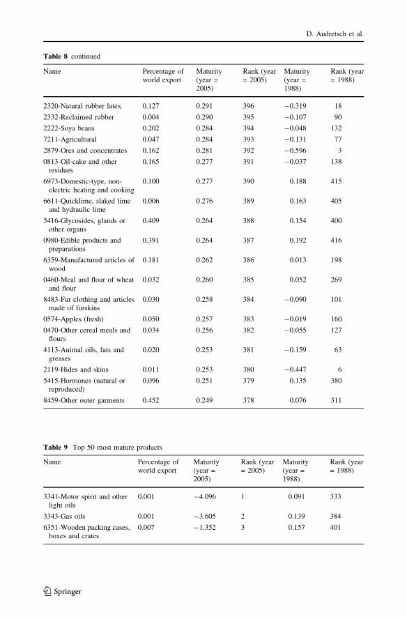
Table 8 continued
Name Percentage ofworld export
Maturity(year =2005)
Rank (year= 2005)
Maturity(year =1988)
Rank (year= 1988)
2320-Natural rubber latex 0.127 0.291 396 -0.319 18
2332-Reclaimed rubber 0.004 0.290 395 -0.107 90
2222-Soya beans 0.202 0.284 394 -0.048 132
7211-Agricultural 0.047 0.284 393 -0.131 77
2879-Ores and concentrates 0.162 0.281 392 -0.596 3
0813-Oil-cake and otherresidues
0.165 0.277 391 -0.037 138
6973-Domestic-type, non-electric heating and cooking
0.100 0.277 390 0.188 415
6611-Quicklime, slaked limeand hydraulic lime
0.006 0.276 389 0.163 405
5416-Glycosides, glands orother organs
0.409 0.264 388 0.154 400
0980-Edible products andpreparations
0.391 0.264 387 0.192 416
6359-Manufactured articles ofwood
0.181 0.262 386 0.013 198
0460-Meal and flour of wheatand flour
0.032 0.260 385 0.052 269
8483-Fur clothing and articlesmade of furskins
0.030 0.258 384 -0.090 101
0574-Apples (fresh) 0.050 0.257 383 -0.019 160
0470-Other cereal meals andflours
0.034 0.256 382 -0.055 127
4113-Animal oils, fats andgreases
0.020 0.253 381 -0.159 63
2119-Hides and skins 0.011 0.253 380 -0.447 6
5415-Hormones (natural orreproduced)
0.096 0.251 379 0.135 380
8459-Other outer garments 0.452 0.249 378 0.076 311
Table 9 Top 50 most mature products
Name Percentage ofworld export
Maturity(year =2005)
Rank (year= 2005)
Maturity(year =1988)
Rank (year= 1988)
3341-Motor spirit and otherlight oils
0.001 -4.096 1 0.091 333
3343-Gas oils 0.001 -3.605 2 0.139 384
6351-Wooden packing cases,boxes and crates
0.007 -1.352 3 0.157 401
D. Audretsch et al.
123
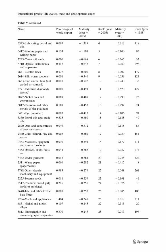
Table 9 continued
Name Percentage ofworld export
Maturity(year =2005)
Rank (year= 2005)
Maturity(year =1988)
Rank (year= 1988)
3345-Lubricating petrol andoils
0.067 -1.319 4 0.212 418
6412-Printing paper andwriting paper
0.124 -1.101 5 -0.100 95
2235-Castor oil seeds 0.000 -0.668 6 -0.267 32
8710-Optical instrumentsand apparatus
0.515 -0.643 7 0.069 298
7641-Electric lines 0.572 -0.600 8 -0.007 179
2614-Silk worm cocoons 0.001 -0.546 9 -0.059 124
2683-Fine animal hair (notcarded or combed)
0.010 -0.542 10 -0.240 35
2771-Industrial diamonds(sorted)
0.007 -0.491 11 0.520 427
2872-Nickel ores andconcentrates
0.069 -0.469 12 -0.290 25
6812-Platinum and othermetals of the platinum
0.189 -0.453 13 -0.292 24
0451-Rye (unmilled) 0.003 -0.413 14 -0.106 91
3330-Petrol oils and crudeoils
9.535 -0.380 15 -0.188 49
2890-Ores and concentratesof precious metals
0.049 -0.372 16 -0.115 87
2440-Cork, natural, raw andwaste
0.003 -0.369 17 -0.030 151
0483-Macaroni, spaghettiand similar products
0.030 -0.294 18 0.177 411
8452-Dresses, skirts, suitsetc.
0.044 -0.285 19 0.057 277
8442-Under garments 0.013 -0.284 20 0.238 422
2511-Waste paper(paperboard)
0.066 -0.282 21 -0.417 8
7788-Other electricmachinery and equipment
0.983 -0.279 22 0.048 261
2225-Sesame seeds 0.011 -0.259 23 -0.198 46
2517-Chemical wood pulp(soda or sulphate)
0.216 -0.255 24 -0.376 10
2640-Jute and other textilebast fibres
0.001 -0.253 25 -0.085 106
7284-Mach and appliances 1.404 -0.248 26 0.019 211
6831-Nickel and nickelalloys
0.107 -0.245 27 -0.315 20
8813-Photographic andcinematographic apparatus
0.370 -0.243 28 0.013 197
International product life cycles, trade and development stages
123
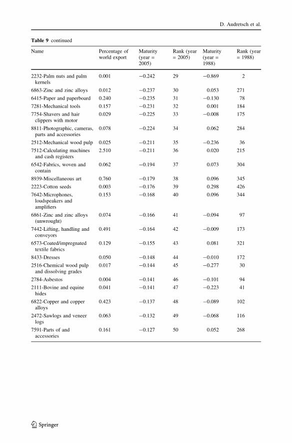
Table 9 continued
Name Percentage ofworld export
Maturity(year =2005)
Rank (year= 2005)
Maturity(year =1988)
Rank (year= 1988)
2232-Palm nuts and palmkernels
0.001 -0.242 29 -0.869 2
6863-Zinc and zinc alloys 0.012 -0.237 30 0.053 271
6415-Paper and paperboard 0.240 -0.235 31 -0.130 78
7281-Mechanical tools 0.157 -0.231 32 0.001 184
7754-Shavers and hairclippers with motor
0.029 -0.225 33 -0.008 175
8811-Photographic, cameras,parts and accessories
0.078 -0.224 34 0.062 284
2512-Mechanical wood pulp 0.025 -0.211 35 -0.236 36
7512-Calculating machinesand cash registers
2.510 -0.211 36 0.020 215
6542-Fabrics, woven andcontain
0.062 -0.194 37 0.073 304
8939-Miscellaneous art 0.760 -0.179 38 0.096 345
2223-Cotton seeds 0.003 -0.176 39 0.298 426
7642-Microphones,loudspeakers andamplifiers
0.153 -0.168 40 0.096 344
6861-Zinc and zinc alloys(unwrought)
0.074 -0.166 41 -0.094 97
7442-Lifting, handling andconveyors
0.491 -0.164 42 -0.009 173
6573-Coated/impregnatedtextile fabrics
0.129 -0.155 43 0.081 321
8433-Dresses 0.050 -0.148 44 -0.010 172
2516-Chemical wood pulpand dissolving grades
0.017 -0.144 45 -0.277 30
2784-Asbestos 0.004 -0.141 46 -0.101 94
2111-Bovine and equinehides
0.041 -0.141 47 -0.223 41
6822-Copper and copperalloys
0.423 -0.137 48 -0.089 102
2472-Sawlogs and veneerlogs
0.063 -0.132 49 -0.068 116
7591-Parts of andaccessories
0.161 -0.127 50 0.052 268
D. Audretsch et al.
123
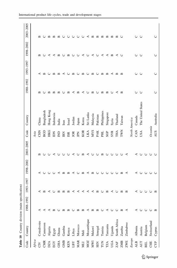
Table
10
Countrydivision(m
ainspecification)
Code
Country
1988–1992
1993–1997
1998–2002
2003–2005
Code
Country
1988–1992
1993–1997
1998–2002
2003–2005
Africa
Asia
CIV
Cotedivoire
AA
AB
CHN
China
BA
BB
CMR
Cam
eroon
AB
CC
BGD
Bangladesh
CB
CC
DZA
Algeria
AA
CC
HKG
HongKong
BC
AB
EGY
Egypt
BC
CA
IDN
Indonesia
BB
AB
GHA
Ghana
CB
AC
IND
India
BB
BB
GMB
Gam
bia
BB
BC
IRN
Iran
CA
CC
KEN
Kenya
BB
BC
ISR
Israel
BC
BC
LBY
Libya
CA
AA
JOR
Jordan
AB
CC
MAR
Morocco
BA
CC
JPN
Japan
BC
CC
MLI
Mali
BA
BB
KOR
Korea
AB
AC
MOZ
Mozambique
AA
AA
LKA
SriLanka
CC
CA
MWI
Malaw
iB
AB
CMYS
Malaysia
BB
AB
SEN
Senegal
BB
CC
PAK
Pakistan
CC
CB
TUN
Tunisia
CC
CB
PHL
Philippines
BB
AB
TZA
Tanzania
AB
CC
SGP
Singapore
BB
AB
UGA
Uganda
CA
CC
SYR
Syria
CA
BB
ZAF
South
Africa
CC
CC
THA
Thailand
AB
AB
ZMB
Zam
bia
BB
BC
TWN
Taiwan
BB
CC
ZWE
Zim
babwe
AB
AA
Europe
NorthAmerica
ALB
Albania
AA
AA
CAN
Canada
CC
CC
AUT
Austria
CC
CC
USA
TheUnited
States
CC
CC
BEL
Belgium
CC
CC
CHE
Switzerland
CC
CC
Oceania
CYP
Cyprus
BB
CC
AUS
Australia
CC
CC
International product life cycles, trade and development stages
123
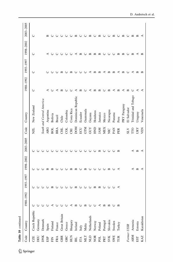
Table
10continued
Code
Country
1988–1992
1993–1997
1998–2002
2003–2005
Code
Country
1988–1992
1993–1997
1998–2002
2003–2005
CZE
Czech
Republic
CC
CC
NZL
New
Zealand
CC
CC
DEU
Germany
CC
CC
DNK
Denmark
CC
CC
South
andCentralAmerica
ESP
Spain
CC
BC
ARG
Argentina
AC
AB
FIN
Finland
AB
BC
BOL
Bolivia
CC
CC
FRA
France
CC
CC
BRA
Brazil
AC
CC
GBR
Great
Britain
CC
CC
CHL
Chile
BB
CC
GRC
Greece
CC
CC
COL
Colombia
CC
CC
HUN
Hungary
AC
BC
CRI
CostaRica
CB
CC
IRL
Ireland
BB
BC
DOM
Dominican
Republic
AC
AB
ITA
Italy
CC
CC
ECU
Ecuador
BC
BC
MLT
Malta
BC
BC
GTM
Guatem
ala
CC
CC
NLD
Netherlands
CC
CC
GUY
Guyana
AA
BB
NOR
Norw
ayC
BC
CHND
Honduras
BB
BC
POL
Poland
AB
CB
JAM
Jamaica
BB
BB
PRT
Portugal
BC
CC
MEX
Mexico
CA
CC
SVK
Slovakia
BC
BC
NIC
Nicaragua
BB
CC
SWE
Sweden
CC
CC
PAN
Panam
aA
BC
B
TUR
Turkey
BA
AB
PER
Peru
BA
BC
PRY
Paraguay
AB
BB
Form
erUSSR
SLV
ElSalvador
BC
CC
ARM
Arm
enia
AA
TTO
Trinidad
andTobago
CA
BB
EST
Estonia
BB
URY
Uruguay
AB
AB
KAZ
Kazakhstan
AA
VEN
Venezuela
AB
BA
D. Audretsch et al.
123
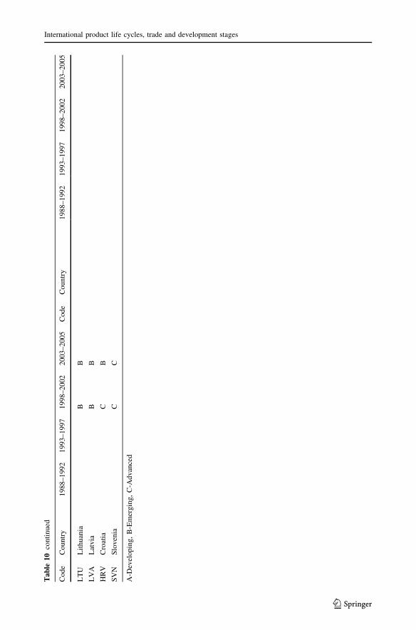
Table
10continued
Code
Country
1988–1992
1993–1997
1998–2002
2003–2005
Code
Country
1988–1992
1993–1997
1998–2002
2003–2005
LTU
Lithuania
BB
LVA
Latvia
BB
HRV
Croatia
CB
SVN
Slovenia
CC
A-D
eveloping,B-Emerging,C-A
dvanced
International product life cycles, trade and development stages
123
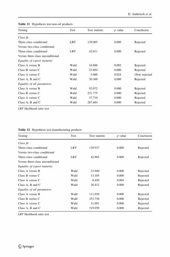
Table 11 Hypothesis test-non-oil products
Testing Test Test statistic p value Conclusion
Class fit
Three-class conditional LRT 139.085 0.000 Rejected
Versus two-class conditional
Three-class conditional LRT 42.011 0.000 Rejected
Versus three-class unconditional
Equality of export maturity
Class A versus B Wald 16.888 0.002 Rejected
Class B versus C Wald 23.894 0.000 Rejected
Class A versus C Wald 5.088 0.024 (Not) rejected
Class A, B and C Wald 30.360 0.000 Rejected
Equality of all parameters
Class A versus B Wald 92.072 0.000 Rejected
Class B versus C Wald 231.775 0.000 Rejected
Class A versus C Wald 37.710 0.000 Rejected
Class A, B and C Wald 287.684 0.000 Rejected
LRT likelihood ratio test
Table 12 Hypothesis test-manufacturing products
Testing Test Test statistic p value Conclusion
Class fit
Three-class conditional LRT 139.937 0.000 Rejected
Versus two-class conditional
Three-class conditional LRT 42.965 0.000 Rejected
Versus three-class unconditional
Equality of export maturity
Class A versus B Wald 23.940 0.000 Rejected
Class B versus C Wald 13.105 0.000 Rejected
Class A versus C Wald 8.450 0.004 Rejected
Class A, B and C Wald 26.412 0.000 Rejected
Equality of all parameters
Class A versus B Wald 111.039 0.000 Rejected
Class B versus C Wald 253.736 0.000 Rejected
Class A versus C Wald 51.091 0.000 Rejected
Class A, B and C Wald 319.959 0.000 Rejected
LRT likelihood ratio test
D. Audretsch et al.
123
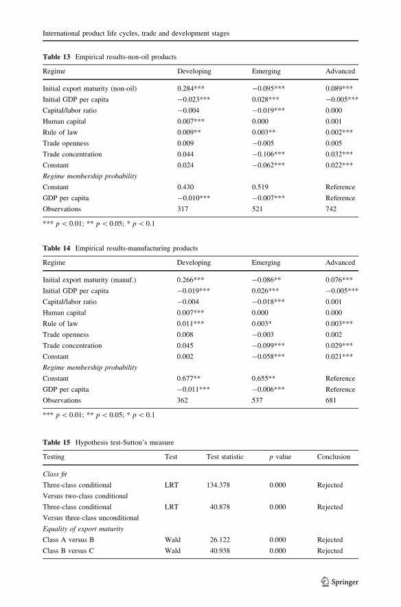
Table 13 Empirical results-non-oil products
Regime Developing Emerging Advanced
Initial export maturity (non-oil) 0.284*** -0.095*** 0.089***
Initial GDP per capita -0.023*** 0.028*** -0.005***
Capital/labor ratio -0.004 -0.019*** 0.000
Human capital 0.007*** 0.000 0.001
Rule of law 0.009** 0.003** 0.002***
Trade openness 0.009 -0.005 0.005
Trade concentration 0.044 -0.106*** 0.032***
Constant 0.024 -0.062*** 0.022***
Regime membership probability
Constant 0.430 0.519 Reference
GDP per capita -0.010*** -0.007*** Reference
Observations 317 521 742
*** p\ 0.01; ** p\ 0.05; * p\ 0.1
Table 14 Empirical results-manufacturing products
Regime Developing Emerging Advanced
Initial export maturity (manuf.) 0.266*** -0.086** 0.076***
Initial GDP per capita -0.019*** 0.026*** -0.005***
Capital/labor ratio -0.004 -0.018*** 0.001
Human capital 0.007*** 0.000 0.000
Rule of law 0.011*** 0.003* 0.003***
Trade openness 0.008 -0.003 0.002
Trade concentration 0.045 -0.099*** 0.029***
Constant 0.002 -0.058*** 0.021***
Regime membership probability
Constant 0.677** 0.655** Reference
GDP per capita -0.011*** -0.006*** Reference
Observations 362 537 681
*** p\ 0.01; ** p\ 0.05; * p\ 0.1
Table 15 Hypothesis test-Sutton’s measure
Testing Test Test statistic p value Conclusion
Class fit
Three-class conditional LRT 134.378 0.000 Rejected
Versus two-class conditional
Three-class conditional LRT 40.878 0.000 Rejected
Versus three-class unconditional
Equality of export maturity
Class A versus B Wald 26.122 0.000 Rejected
Class B versus C Wald 40.938 0.000 Rejected
International product life cycles, trade and development stages
123
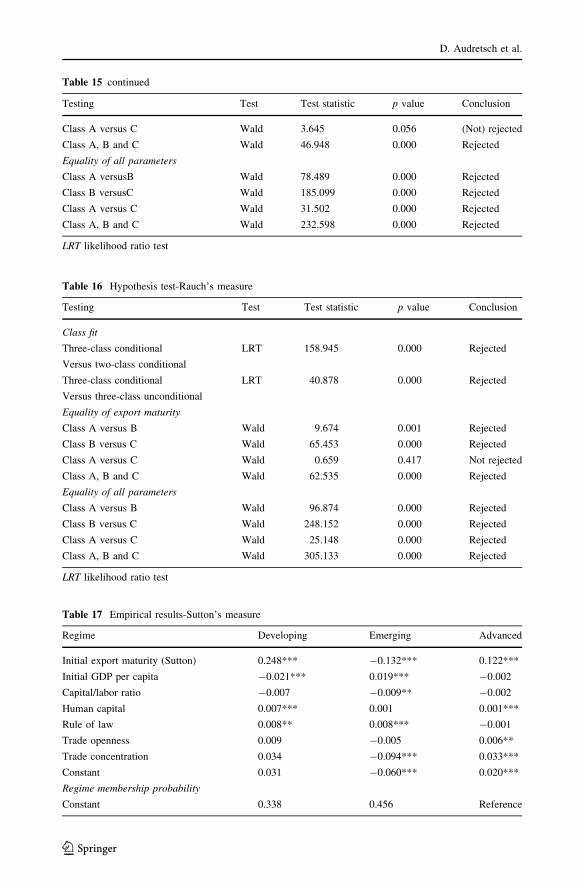
Table 16 Hypothesis test-Rauch’s measure
Testing Test Test statistic p value Conclusion
Class fit
Three-class conditional LRT 158.945 0.000 Rejected
Versus two-class conditional
Three-class conditional LRT 40.878 0.000 Rejected
Versus three-class unconditional
Equality of export maturity
Class A versus B Wald 9.674 0.001 Rejected
Class B versus C Wald 65.453 0.000 Rejected
Class A versus C Wald 0.659 0.417 Not rejected
Class A, B and C Wald 62.535 0.000 Rejected
Equality of all parameters
Class A versus B Wald 96.874 0.000 Rejected
Class B versus C Wald 248.152 0.000 Rejected
Class A versus C Wald 25.148 0.000 Rejected
Class A, B and C Wald 305.133 0.000 Rejected
LRT likelihood ratio test
Table 17 Empirical results-Sutton’s measure
Regime Developing Emerging Advanced
Initial export maturity (Sutton) 0.248*** -0.132*** 0.122***
Initial GDP per capita -0.021*** 0.019*** -0.002
Capital/labor ratio -0.007 -0.009** -0.002
Human capital 0.007*** 0.001 0.001***
Rule of law 0.008** 0.008*** -0.001
Trade openness 0.009 -0.005 0.006**
Trade concentration 0.034 -0.094*** 0.033***
Constant 0.031 -0.060*** 0.020***
Regime membership probability
Constant 0.338 0.456 Reference
Table 15 continued
Testing Test Test statistic p value Conclusion
Class A versus C Wald 3.645 0.056 (Not) rejected
Class A, B and C Wald 46.948 0.000 Rejected
Equality of all parameters
Class A versusB Wald 78.489 0.000 Rejected
Class B versusC Wald 185.099 0.000 Rejected
Class A versus C Wald 31.502 0.000 Rejected
Class A, B and C Wald 232.598 0.000 Rejected
LRT likelihood ratio test
D. Audretsch et al.
123
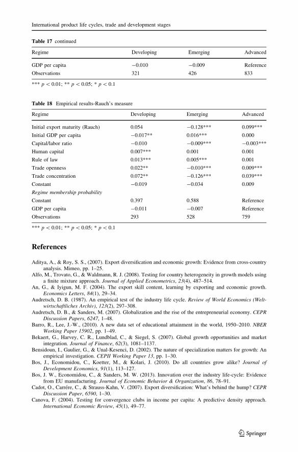
References
Aditya, A., & Roy, S. S., (2007). Export diversification and economic growth: Evidence from cross-countryanalysis. Mimeo, pp. 1–25.
Alfo, M., Trovato, G., & Waldmann, R. J. (2008). Testing for country heterogeneity in growth models usinga finite mixture approach. Journal of Applied Econometrics, 23(4), 487–514.
An, G., & Iyigun, M. F. (2004). The export skill content, learning by exporting and economic growth.Economics Letters, 84(1), 29–34.
Audretsch, D. B. (1987). An empirical test of the industry life cycle. Review of World Economics (Welt-wirtschaftliches Archiv), 123(2), 297–308.
Audretsch, D. B., & Sanders, M. (2007). Globalization and the rise of the entrepreneurial economy. CEPRDiscussion Papers, 6247, 1–48.
Barro, R., Lee, J.-W., (2010). A new data set of educational attainment in the world, 1950–2010. NBERWorking Paper 15902, pp. 1–49.
Bekaert, G., Harvey, C. R., Lundblad, C., & Siegel, S. (2007). Global growth opportunities and marketintegration. Journal of Finance, 62(3), 1081–1137.
Bensidoun, I., Gaulier, G., & Unal-Kesenci, D. (2002). The nature of specialization matters for growth: Anempirical investigation. CEPII Working Paper 13, pp. 1–30.
Bos, J., Economidou, C., Koetter, M., & Kolari, J. (2010). Do all countries grow alike? Journal ofDevelopment Economics, 91(1), 113–127.
Bos, J. W., Economidou, C., & Sanders, M. W. (2013). Innovation over the industry life-cycle: Evidencefrom EU manufacturing. Journal of Economic Behavior & Organization, 86, 78–91.
Cadot, O., Carrere, C., & Strauss-Kahn, V. (2007). Export diversification: What’s behind the hump? CEPRDiscussion Paper, 6590, 1–30.
Canova, F. (2004). Testing for convergence clubs in income per capita: A predictive density approach.International Economic Review, 45(1), 49–77.
Table 18 Empirical results-Rauch’s measure
Regime Developing Emerging Advanced
Initial export maturity (Rauch) 0.054 -0.128*** 0.099***
Initial GDP per capita -0.017** 0.016*** 0.000
Capital/labor ratio -0.010 -0.009*** -0.003***
Human capital 0.007*** 0.001 0.001
Rule of law 0.013*** 0.005*** 0.001
Trade openness 0.022** -0.010*** 0.009***
Trade concentration 0.072** -0.126*** 0.039***
Constant -0.019 -0.034 0.009
Regime membership probability
Constant 0.397 0.588 Reference
GDP per capita -0.011 -0.007 Reference
Observations 293 528 759
*** p\ 0.01; ** p\ 0.05; * p\ 0.1
Table 17 continued
Regime Developing Emerging Advanced
GDP per capita -0.010 -0.009 Reference
Observations 321 426 833
*** p\ 0.01; ** p\ 0.05; * p\ 0.1
International product life cycles, trade and development stages
123
Chadha, A. (2009). Product cycles, innovation, and exports: A study of indian pharmaceuticals. WorldDevelopment, 37(9), 1478–1483.
Choung, J.-Y., Hwang, H.-R., & Song, W. (2014). Transitions of innovation activities in latecomer coun-tries: An exploratory case study of South Korea. World Development, 54(C), 156–167.
Cline, W. R. (1982). Can the East Asian model of development be generalized? World Development, 10(2),81–90.
Cline, W. R. (2010). Exports of manufactures and economic growth: The fallacy of composition revisited.In: Spence, M., Leipziger, D. (Eds.), Globalization and growth: Implication for a post-crisis world,pp. 195–234.
Connolly, M. (1999). North-south technological diffusion: A new case for dynamic gains from trade. DukeUniversity Department of Economics Working Paper 99-08.
Dalum, B., Laursen, K., & Verspagen, B. (1999). Does specialization matter for growth? Industrial andCorporate Change, 8(2), 267–88.
de Pineres, S. A. G., & Ferrantino, M. (1997). Export diversification and structural dynamics in the growthprocess: The case of Chile. Journal of Development Economics, 52(2), 375–391.
Dollar, D. (1986). Product cycle in the North-South trade. American Economic Review, 76, 177–190.Durlauf, S. N., Johnson, P., & Temple, J. (2005). Growth econometrics. In: Aghion, P., Durlauf, S. (Eds.),
Handbook of economic growth, 1st edn. Vol. 1, Part A. Elsevier, Chapter 08, pp. 555–677.Durlauf, S. N., & Johnson, P. A. (1995). Multiple regimes and cross-country growth behaviour. Journal of
Applied Econometrics, 10(4), 365–384.Feenstra, R. C., & Rose, A. K. (2000). Putting things in order: Trade dynamics and product cycles. The
Review of Economics and Statistics, 82(3), 369–382.Flam, H., & Helpman, E. (1987). Vertical product differentiation and North-South trade. American Eco-
nomic Review, 77, 810–822.Giles, J. A., & Williams, C. L. (2000). Export-led growth: A survey of the empirical literature and some
non-causality results. Part 2. Journal of International Trade & Economic Development, 9(4), 445–470.Greene, W. (2007). LIMDEP, Version 9.0: Reference Guide. Econometric Software, Inc.Grossman, G., & Helpman, E. (1991). Quality ladders and product cycles. Quarterly Journal of Economics,
109, 557–586.Gylfason, T. (2004). Natural resources and economic growth: From dependence to diversification. CEPR
Discussion Papers, 4804(4804), 1–34.Hall, R. E., & Jones, C. I. (1999). Why do some countries produce so much more output per worker than
others? The Quarterly Journal of Economics, 114(1), 83–116.Hallak, J. C. (2006). Product quality and the direction of trade. Journal of International Economics, 68(1),
238–265.Hallak, J. C., & Schott, P. K. (2011). Estimating cross-country differences in product quality. The Quarterly
Journal of Economics, 126(1), 417–474.Hausmann, R., & Hidalgo, C. (2011). The network structure of economic output. Journal of Economic
Growth, 16(4), 309–342.Hausmann, R., Hwang, J., & Rodrik, D. (2007). What you export matters. Journal of Economic Growth,
12(1), 1–25.Herzer, D., & Nowak-Lehnmann, F. (2006). What does export diversification do for growth? An econo-
metric analysis. Applied Economics, 38(15), 1825–1838.Hesse, H. (2008). Export diversification and economic growth. The World Bank Commission on Growth and
Development Working Paper 21, pp. 1–25.Hidalgo, C., & Hausmann, R. (2009). The buliding blocks of economic complexitity. Proceedings of the
National Academy of Science of the United States of America, 106(26), 10570–10575.Hidalgo, C. A., Klinger, B., Barabasi, A.-L., & Hausmann, R. (2007). The product space conditions the
development of nations. Science, 317(5837), 482–487.Hirsch, S. (1967). Location of Industry and International Competitiveness. Oxford: Oxford University Press.Hobday, M. (1995). East asian latecomer firms: Learning the technology of electronics.World Development,
23(7), 1171–1193.Hobday, M., Rush, H., & Bessant, J. (2004). Approaching the innovation frontier in Korea: The transition
phase to leadership. Research Policy, 33(10), 1433–1457.Imbs, J., & Wacziarg, R. (2003). Stages of diversification. The American Economic Review, 93(1), 63–86.Indjikian, R., & Siegel, D. S. (2005). The impact of investment in IT on economic performance: Impli-
cations for developing countries. World Development, 33(5), 681–700.Jarreau, J., & Poncet, S. (2012). Export sophistication and economic growth: Evidence from China. Journal
of Development Economics, 97(2), 281–292.
D. Audretsch et al.
123
Jensen, R., & Thursby, M. (1986). A strategic approach to the product cycle. Journal of InternationalEconomics, 21, 269–284.
Kellman, M., & Landau, D. (1984). The nature of Japan’s comparative advantage, 1965–80. WorldDevelopment, 12(4), 433–438.
Khandelwal, A. (2010). The long and short (of) quality ladders. Review of Economic Studies, 77(4),1450–1476.
Klepper, S. (1996). Entry, exit, growth, and innovation over the product life cycle. American EconomicReview, 86(3), 562–83.
Klinger, B., & Lederman, D. (2006). Diversification, innovation, and imitation inside the global techno-logical frontier. The World Bank Policy Research Working Paper Series 3872, pp. 1–24.
Krugman, P. (1979). A model of innovation, technology transfer, and the world distribution of income.Journal of Political Economy, 87(2), 253–266.
Lai, E. (1995). The product cycle and the world distribution of income: A reformulation. Journal ofInternational Economics, 39, 369–382.
Lederman, D., & Maloney, W. F. (2012). Does what you export matter? In Search of empirical guidance forindustrial policies. No. 9371 in World Bank Publications. The World Bank.
Lee, J. (2011). Export specialization and economic growth around the world. Economic Systems, 35(1),45–63.
Lee, J.-W. (1995). Capital goods imports and long-run growth. Journal of Development Economics, 48(1),91–110.
Levine, R., & Renelt, D. (1992). A sensitivity analysis of cross-country growth regressions. AmericanEconomic Review, 82(4), 942–63.
Lewer, J., & den Berg, H. V. (2003). Does trade composition influence economic growth? Time seriesevidence for 28 OECD and developing countries. Journal of International Trade & EconomicDevelopment, 12(1), 39–96.
Martin, W. (1993). The fallacy of composition and developing country exports of manufactures. The WorldEconomy, 16(2), 159–172.
Moschos, D. (1989). Export expansion, growth and the level of economic development: An empiricalanalysis. Journal of Development Economics, 30, 93–102.
Mullor-Sebastian, A. (1983). The product life cycle theory: Empirical evidence. Journal of InternationalBusiness Studies, 14, 95–105.
OECD (2005). Micro-policies for growth and productivity: Final report. Technical report, OECD, Paris.Owen, A., Videras, J., & Davis, L. (2009). Do all countries follow the same growth process? Journal of
Economic Growth, 14(4), 265–286.Owen, A. L., & Videras, J. (2012). The quality of growth. MPRA Paper 38342, University Library of
Munich, Germany.Paap, R., Franses, P. H., & van Dijk, D. (2005). Does Africa grow slower than Asia, Latin America and the
Middle East? Evidence from a new data-based classification method. Journal of Development Eco-nomics, 77(2), 553–570.
Pan, H., & Kohler, J. (2007). Technological change in energy systems: Learning curves, logistic curves andinput–output coefficients. Ecological Economics, 63(4), 749–758.
Papageorgiou, C. (2002). Trade as a threshold variable for multiple regimes. Economics Letters, 77(1),85–91.
Pietrobelli, C., & Rabellotti, R. (2011). Global value chains meet innovation systems: Are there learningopportunities for developing countries? World Development, 39(7), 1261–1269.
Ranis, G. (1985). Can the East Asian model of development be generalized? A comment. World Devel-opment, 13(4), 543–545.
Rauch, J. E. (1999). Networks versus markets in international trade. Journal of International Economics,48(1), 7–35.
Redding, S. (2002). Specialization dynamics. Journal of International Economics, 58, 299–334.Rodriguez, F., & Rodrik, D. (2001). Trade policy and economic growth: A skeptic’s guide to the cross-
national evidence. NBER Macroeconomics Annual, 15, 261–338.Sachs, J. D., & Warner, A. (1995). Economic reform and the process of global integration. Brookings Papers
on Economic Activity, 26(1), 1–118.Schneider, P. H. (2005). International trade, economic growth and intellectual property rights: A panel data
study of developed and developing countries. Journal of Development Economics, 78(2), 529–547.Schott, P. K. (2004). Across-product versus within-product specialization in international trade. The
Quarterly Journal of Economics, 119(2), 646–677.Singh, T. (2010). Does international trade cause economic growth? A survey. The World Economy, 33(11),
1517–1564.
International product life cycles, trade and development stages
123
Sutton, J., & Trefler, D. (2011). Deductions from the export basket: Capabilities, wealth and trade. NBERWorking Papers 16834, National Bureau of Economic Research, Inc.
Temple, J. (1999). The new growth evidence. Journal of Economic Literature, 37(1), 112–156.Vaio, G. D., & Enflo, K. (2011). Did globalization drive convergence? Identifying cross-country growth
regimes in the long run. European Economic Review, 55(6), 832–844.Vernon, R. (1966). International investment and international trade in the product cycle. The Quarterly
Journal of Economics, 80(2), 190–207.Wacziarg, R., & Welch, K. H. (2008). Trade liberalization and growth: New evidence. World Bank Eco-
nomic Review, 22(2), 187–231.Worz, J. (2005). Skill intensity in foreign trade and economic growth. Empirica, 32(1), 117–144.Xuefeng, Q., & Yasar, M. (2016). Export market diversification and firm productivity: Evidence from a
large developing country. World Development, 82(C), 28–47.
D. Audretsch et al.
123