NATIVE INTERNAL MIGRATION AND THE LABOR MARKET IMPACT OF IMMIGRATION

George J. Borjas Harvard University

May 2004

1

NATIVE INTERNAL MIGRATION AND THE LABOR MARKET IMPACT OF IMMIGRATION

George J. Borjas

Abstract

Immigrants tend to cluster in a small number of geographic areas. Many studies use this

clustering to estimate the wage impact of immigration by relating wage rates across labor

markets to some measure of immigrant penetration. These spatial correlations may not measure

the true impact of immigration because the internal migration response of native workers helps to

re-equilibrate local labor markets. This paper presents a theoretical and empirical study of how

immigrant supply shocks influence the joint determination of wages and internal migration

decisions in local labor markets. The data indicate that immigration is associated with lower

wages, lower in-migration rates, higher out-migration rates, and a decline in the growth rate of

the native workforce. The native migration response is sufficiently strong to attenuate the

measured impact of immigration on wages in a local labor market from 40 to 60 percent,

depending on whether the labor market is defined at the state or metropolitan area level.

2

NATIVE INTERNAL MIGRATION AND THE LABOR MARKET IMPACT OF IMMIGRATION

George J. Borjas*

I. Introduction

Immigrants in the United States cluster in a small number of geographic areas. In 2000,

for example, 69.2 percent of working-age immigrants resided in six states (California, New

York, Texas, Florida, Illinois, and New Jersey), but only 33.7 percent of natives lived in those

states. Similarly, 38.4 percent of immigrants lived in four metropolitan areas (New York, Los

Angeles, Chicago, and San Francisco), but only 12.2 percent of natives lived in the four

metropolitan areas with the largest native-born populations (New York, Chicago, Los Angeles,

and Philadelphia).

Economic theory suggests that immigration into a closed labor market affects the wage

structure in that market by lowering the wage of competing workers and raising the wage of

complements. Most of the empirical studies in the literature exploit the geographic clustering of

immigrants to measure the labor market impact of immigration by defining the labor market

along a geographic dimension—such as a state or a metropolitan area. Beginning with Grossman

(1982), the typical study regresses a measure of native economic outcomes in the locality (or the

change in that outcome) on the relative quantity of immigrants in that locality (or the change in

* Robert W. Scrivner Professor of Economics and Social Policy, Kennedy School of Government, Harvard

University; and Research Associate, National Bureau of Economic Research. I am grateful to the Smith-Richardson Foundation for research support.

3

the relative number).1 The regression coefficient, or “spatial correlation,” is then interpreted as

the impact of immigration on the native wage structure.

There are two well-known problems with this approach. First, immigrants may not be

randomly distributed across labor markets. If immigrants tend to cluster in areas with thriving

economics, there would be a spurious positive correlation between immigration and area

outcomes either in the cross-section or in the time-series. This spurious correlation could

attenuate or reverse whatever measurable negative effects immigrants might have had on the

wage of competing native workers.2

The second problem is that natives may respond to the entry of immigrants into a local

labor market by moving their labor or capital to other localities until native wages and returns to

capital are again equalized across areas. A large immigrant flow arriving in Los Angeles might

result in, say, fewer workers from Iowa or Ohio moving to California, and a reallocation of

capital across states. An interstate comparison of the wage of native workers might show little or

no difference because the effects of immigration are diffused throughout the national economy,

and not because immigration had no economic effects.

In view of these potential problems it is not too surprising that the empirical literature has

produced a confusing array of results. The measured impact of immigration on the wage of

native workers in local labor markets fluctuates widely from study to study, but seems to cluster

around zero. In recent work (Borjas, 2003), I show that by defining the labor market at the

1 See also Altonji and Card (1991), Borjas (1987), Card (2001), LaLonde and Topel (1991), and Schoeni

(1997). De New and Zimmermann (1994) and Pischke and Velling (1997) provide similar studies for the German labor market. Card’s (1990) case study of the impact of the Mariel immigrant flow into Miami is certainly the most influential study of this type. Friedberg and Hunt (1995) provide a good survey of the literature.

2 Borjas (2001) argues that income-maximizing immigrants would tend to cluster in high-wage regions, helping to move the labor market towards a long-run equilibrium. The evidence does indeed suggest that, within education groups, new immigrants tend to locate in those states that offer the highest rate of return for their skills.

4

national level—which more closely approximates the theoretical counterpart of a closed labor

market—the measured wage impact of immigration becomes much larger. By examining the

evolution of wages in the 1960-2000 period within narrow skill groups (defined in terms of

schooling and labor market experience), I concluded that an immigrant supply shock that

increases the number of workers in a particular skill group by 10 percent reduces the wage of

that skill group by 3 to 4 percent.

In this paper, I explore the disparate findings implied by the two approaches by focusing

on a particular adjustment mechanism that native workers may use to avoid the adverse impacts

of immigration on local labor markets: internal migration. A number of studies already examine

if native migration decisions respond to immigrant supply shocks. As with the spatial correlation

literature, these studies offer a cornucopia of findings, with some studies finding strong effects

(e.g., Frey, 1995, and Borjas, Freeman, and Katz, 1997), and other studies finding little

connection (Card, 2001; and Wright, Ellis, and Reibel, 1997).3

This paper can be viewed as a synthesis of two related, but so far unconnected, strands in

the literature. I present and estimate a theoretical framework that jointly models wage

determination in local labor markets and the native migration decision. The theory yields

estimable equations that explicitly link the parameters measuring the wage impact of

immigration at the national level, the spatial correlation between wages and immigration in local

labor markets, and the native migration response. The model clearly shows that the larger the

native migration response, the greater will be the difference between the estimates of the national

wage effect and the spatial correlation. The model also implies that it is possible to use the

3 Other studies include Card and DiNardo (2000), Filer (1992), and White and Hunter (1993).

5

spatial correlations to calculate the “true” national impact of immigration as long as one has

information on the elasticity measuring the migration response of native workers.

I use data drawn from all the Census cross-sections between 1960 and 2000 to estimate

the key parameters of the model. The data indicate that the measured wage impact of

immigration depends intimately on the geographic definition of the labor market, and is larger as

one expands the size of the market—from the metropolitan area, to the state, to the Census

division, and ultimately to the nation. In contrast, although the measured impact of immigration

on native migration rates also depends on the geographic definition of the labor market, these

effects become smaller as one expands the size of the market. These mirror-image patterns

suggest that the wage effects of immigration on local labor markets are more attenuated the

easier that natives find it to “vote with their feet.” In fact, the native migration response can

account for between 40 and 60 percent of the difference in the measured wage impact of

immigration between the national and local labor market levels, depending on whether the local

labor market is defined by a state or by a metropolitan area.

II. Theory

I use a simple economic model of the joint determination of the regional wage structure

and the internal migration decision of native workers to show the types of parameters that spatial

correlations identify, and to determine if these parameters can be used to identify the national

labor market impact of immigration.4 Suppose that the labor demand function for workers in skill

group i residing in geographic area j at time t can be written as:

4 The model can be viewed as an application of the Blanchard and Katz (1992) framework that analyzes

how local labor markets respond to demand shocks. The basic model presented here builds on a framework developed by Borjas, Freeman, and Katz (1997, unpublished appendix), and further elaborated in Borjas (1999). The

6

(1) ,ijt ijt ijtw X Lη=

where wijt is the wage of workers in cell (i, j, t); Xijt is a demand shifter; Lijt gives the total

number of workers (both immigrants, Mijt, and natives, Nijt); and η is the factor price elasticity

(with η < 0). It is convenient to interpret the elasticity η as the “true” impact that an immigrant

supply shock would have in a closed labor market in the short run, a labor market where neither

capital nor labor responds to the immigrant influx.

For simplicity, I assume that the demand shifter is both time-invariant and region-

invariant (Xijt = Xi). This simplification implies that (within a particular skill group) wages differ

across regions only when the stock of workers is not evenly distributed across regions. The

extension of the model to incorporate differences in the level of the demand curve would

complicate the presentation without substantially altering the basic insights provided by the

model.5 I also assume that the total number of native workers in a particular skill group in the

national economy is fixed at .iN It would not be difficult (though it would be cumbersome) to

extend the model to allow for differential rates of growth in the size of the native workforce.

Suppose that Nij,-1 native workers in skill group i reside in region j in the pre-immigration

period (t = −1). The sorting of native workers across regions in the pre-immigration regime does

not represent a long-run equilibrium; some regions have too many workers and other regions too

presentation here differs from the earlier iterations in a number of ways, particularly by incorporating the presence of internal migration flows before the immigrant supply shock occurs and by deriving estimable equations that can be used to empirically identify the various theoretical parameters.

5 The assumption that the demand shifter is time-invariant implies that the immigrant influx will necessarily lower the average wage in the economy. This assumption could be relaxed by allowing for endogenous capital growth (or for capital flows from abroad).

7

few. The regional wage differentials induce a migration response by native workers even prior to

the immigrant supply shock. In particular, region j experiences a net migration of ∆Nij0 natives

belonging to skill group i between t = −1 and t = 0.

Beginning at time 0, the local labor market (as defined by a particular skill-region cell)

experiences an immigrant supply shock of Mijt immigrants. This immigrant supply shock

continues in all subsequent periods. A convenient assumption that greatly simplifies the

presentation is that region j receives the same number of immigrants in each year. The annual

immigrant influx for a particular skill-region cell can then be represented by Mij. The assumption

that the immigrant supply shock is constant over time is not grossly contradicted by the data for

the United States because the same regions have been the recipients of similar types of

immigrants for several decades.6

For simplicity, I assume that immigrants do not migrate internally within the United

States—they enter region j and remain there.7 Natives continue to make relocation decisions, and

region j experiences a net migration of ∆Nij1 natives in period 1, ∆Nij2 natives in period 2, and so

on. The labor demand function given by equation (1) implies that the wage for skill group i in

region j at time t is then given by:

(2) log wijt = log Xi + η log [Nij,-1 + (t + 1)Mij + ∆Nij0 + ∆Nij1 + . . . + ∆Nijt],

which can be rewritten as:

6 The model could be easily extended to incorporate a time-variant immigrant supply shock to each region

as long as the growth rate of the immigrant influx was constant.

8

(3) log wijt ≈ log wij,-1 + η [(t + 1) mij + vij0 + vij1+ … + vijt ], for t ≥ 0,

where mij = Mij / Nij,-1, the relative number of immigrants entering region j in each period; and vijt

= ∆Nijt / Nij,-1, the net migration rate of natives (relative to the initial population in the region).

Note that wij,-1 gives the initial wage offered to workers in cell (i, j) in the pre-immigration

period.

I assume that the internal migration response of native workers occurs with a lag. For

example, immigrants begin to arrive at t = 0. The demand function in equation (3) implies that

the wage response to immigration is immediate, so that wages fall in the immigrant-penetrated

regions. The migration decisions of natives induced by this supply shock, however, are not

observed until the next period. The lagged supply response that describes the migration decisions

of native workers is given by:

(4) vijt = σ (log wij,t-1 – log w−i,t-1),

where σ is the supply elasticity (σ > 0); and log w−i,t-1 is the equilibrium wage (for skill group i)

that will be observed throughout the national economy once all migration responses to the

immigrant supply shocks that have occurred up to time t − 1 have been made.8 It might seem

7 The evidence reported in Bartel (1989) suggests that the internal migration decisions of immigrants in the

United States do not seem to be very sensitive to regional wage differences, but are instead more sensitive to the location decisions of earlier immigrant waves.

8 More precisely, log w−i,t-1 = log w−i,-1 + η(tmi), where mi gives the per-period number of immigrants in skill group i relative to the total number of natives in that skill group. Note that the model implicitly assumes that the native population is large enough (relative to the total immigrant supply shock) to be able to equalize the number of workers across labor markets through internal migration.

9

preferable to model the supply function so that natives take into account the expected impact of

future immigration. However, the total supply shock up to time t − 1 is a “sufficient statistic”

because we have assumed that the region receives the same number of immigrants in every

period.

The model does not impose any restrictions on the value of the parameter σ (except that it

is positive). If σ is sufficiently “small,” the migration response of natives may not be completed

within one period. Some workers may respond immediately, but other workers will take

somewhat longer.9 Note also that the migration decision is made by comparing the current wage

in region j to the wage that region j will eventually attain. In this model, therefore, there is

perfect information about the eventual outcome that results from the accumulation of immigrant

supply shocks. Unlike the typical cobweb model, persons are not making decisions based on

erroneous information. The lags arise simply because it is difficult to change locations

immediately.

As noted above, the existence of regional wage differentials at time t = −1 implies that

native internal migration was taking place even prior to the immigrant supply shock. It is useful

to describe the determinants of the net migration flow vij0. In the pre-immigration period, the

equilibrium wage that would be eventually attained in the economy is:

(5) log w−i,-1 = Xi + η log *iN ,

9 In a sense, the migration behavior underlying equation (4) is analogous to the firm’s behavior in the

presence of adjustment costs (Hamermesh, 1993). One can justify this staggered response in a number of ways. The labor market is in continual flux, with persons entering and leaving the market. Because migration is costly, workers may find it optimal to time the lumpy migration decision concurrently with these transitions. Workers may also face

10

where *iN represent the number of native workers in skill group i that would live in each region

once long-run equilibrium is attained.10 The pre-existing net migration rate of native workers is

then given by:

(6) vij0 = σ (log wij,-1 – log w−i,-1) = ησ λij,

where *, 1log( / ).ij ij iN N−λ = By definition, the variable λij is negative when the initial wage in

region j is higher than the long-run equilibrium wage (in other words, there are fewer workers in

region j than there will be after all internal migration takes place). Equation (6) then implies that

the net migration rate in region j is positive (since η < 0).

Native net migration continues after the immigrant supply shock. In the mathematical

appendix, I show that the native net-migration rate at year t can be written as:

(7) vijt = ησ (1 + ησ)t λij + [1 – (1 + ησ)t] mi - [1 – (1 + ησ)t] mij ,

where / ,i i im M N= and Mi gives the per-period number of immigrants in skill group i. The

restriction 0 < (1 + ησ) < 1 is assumed to hold throughout the analysis.

The total number of native workers in cell (i, j, t) is then given by the sum of the initial

stock (Nij,-1) and the net migration flows defined by equation (7), or:

constraints that prevent them from taking immediate advantage of regional wage differentials, including various forms of “job-lock” or short-term liquidity constraints.

11

(8)

1, 1log log [(1 ) 1]

(1 ) [1 (1 ) ]1 ( 1)

(1 ) [1 (1 ) ] ,1 ( 1)

tijt ij ij

t

it

t

ijt

N N

t mt t

t mt t

+−= + + ησ − λ

+ ησ − + ησ+ + + ησ +

+ ησ − + ησ− + + ησ +

where ( 1) ,it im t m= + the relative number of immigrants with skill i who have migrated to the

United States as of time t; and ( 1) ,ijt ijm t m= + the relative number of immigrants with skill i who

have migrated to region j as of time t.11 The wage for workers in cell (i, j, t) is then given by:

(9)

1, 1log log [(1 ) 1]

(1 ) [1 (1 ) ]1 ( 1)

1 (1 ) [1 (1 ) ] .1 ( 1)

tijt ij ij

t

it

t

ijt

w w

t mt t

mt t

+−= + η + ησ − λ

+ ησ − + ησ− η + + ησ +

+ ησ − + ησ+ η − + ησ +

Consider equation (8), which describes the evolution of the size of the native workforce

in a particular labor market. In addition to the initial size of the workforce, the current stock of

native workers in cell (i, j, t) depends on three factors. First, there is a term in λij that essentially

gives the total net migration rate of natives that would have occurred in the absence of

immigration. Second, there is a term that relates the size of the native workforce to the total

immigrant supply shock in skill group i. The last term indicates how the current size of the native

10 This number, of course, equals the total number of natives in a skill group divided by the number of

regions.

11 A tilde above a variable indicating the size of the immigrant supply shock implies that the variable refers to the entire stock of immigrants up to a particular point in time (rather than to the per-period flow).

12

workforce depends on the size of the total region-specific immigrant supply shock. Equation (9)

shows that the same three variables also affect the evolution of wages in the local labor market.

Equations (8) and (9) have a number of implications for empirical studies of the impact

of immigration on native migration decisions or wages. Consider the behavior of the coefficients

of the region-specific immigrant supply shock variable in the size of the native workforce and

wage regressions. As t grows large, the coefficient in the native workforce regression (which

should be negative) converges to –1, while the coefficient in the wage regression (which should

also be negative) converges to zero. Put differently, the longer the time elapsed between the

beginning of the immigrant supply shock and the measurement of native migration decisions and

native wages, the more likely that natives have completely internalized the immigrant supply

shock and the less likely that the spatial correlation approach will uncover any wage effect on

local labor markets.

Most important, the coefficients of the region-specific (total) immigrant supply shock in

the two equations can be used to identify the parameter of interest, η. In fact, these two

coefficients indicate how the spatial correlation (i.e., the impact of immigration on wages that

can be estimated by comparing local labor markets) relates to the national wage impact of

immigration, the factor price elasticity η. In particular, let γNt be the coefficient of the immigrant

supply shock in the native workforce regression estimated at time t, and let γWt be the respective

coefficient in the wage regression. The definitions of these coefficients imply that:

(10) γWt = η (1 + γNt).

13

It is easy to show that the coefficient γNt gives the number of natives who migrate out of a

particular labor market for every immigrant who migrates there (i.e., /Nt tN Mγ =∂ ∂ ). In effect,

the factor price elasticity measuring the impact of immigration in the closed national labor

market can be estimated from the spatial correlation by “blowing up” the coefficient from the

cross-region wage regression by taking into account the relative number of natives who stay. To

illustrate, suppose that the coefficient γNt is -0.5, indicating that 5 fewer natives choose to reside

in the local labor market for every 10 immigrants that enter that market. Equation (10) then

implies that the spatial correlation that can be estimated by comparing native wages across local

labor markets is only half the size of the true factor price elasticity.

Empirical Specification

In the next section, I will use data drawn from the 1960-2000 Censuses to estimate the

key parameters of the model. These data, in essence, provide five wage and size-of-workforce

observations (one for each Census cross-section) for labor markets defined by skill groups and

geographic regions. The available data, therefore, are not sufficiently detailed to allow me to

estimate the dynamic evolution of the size of the native workforce and wages as summarized by

equations (8) and (9). These equations, after all, have time-varying coefficients for the variable

measuring the immigrant supply shock, and these coefficients are highly nonlinear in time. I

derive a simpler framework that can be applied to the available data by using the Taylor’s

approximation (1 + x)t ≈ (1 + xt). Equations (8) and (9) can then be rewritten as:12

12 I also use the approximation that t is relatively large so that the ratio t/(t +1) ≈ 1 and 1/t ≈ 0; in other

words, the wage convergence process has been going on for some time before we observe the data points.

14

(11) log Nijt = log Nij,-1 + ησ λij + ησ (t λij) – ησ itm + ησ ijtm ,

(12) log wijt = log wij,-1 + η2 σ λij + η2 σ (t λij) – ησ itm + η(1 + ησ) ijtm .

These equations can be estimated by stacking the available data on the size of the native

workforce, wages, and immigrant supply shocks across skill groups, regions, and time. Many of

the regressors in equations (11) and (12) can then be absorbed by including appropriately defined

vectors of fixed effects in the regressions. For example, the inclusion of fixed effects indicating

skill-region cells absorbs the vector of variables (Nij,-1, λij) in equation (11) and the vector (wij,-1,

λij) in equation (12). Similarly, interactions between skill and time fixed effects absorb the

variable itm in both equations.

In addition to these fixed effects, the regression models in (11) and (12) indicate the

presence of two regressors that vary by skill, region, and time. The first, of course, is the region-

specific immigrant supply shock, the key independent variable in any empirical analysis that

attempts to estimate spatial correlations. Note that the region-specific immigrant supply shock

gives the total number of immigrants who have arrived in the region up to time t relative to the

(initial) native population.

The second is the variable (t λij), which is related to the (total) net migration rate of

natives that would have been observed as of time (t – 1) had there been no immigration. This

variable is not observable. In the empirical work reported below, I proxy for this variable by

including in the regression either a lagged measure of the number of natives in the workforce or

the lagged growth rate of the native workforce in the particular labor market.

The regression models in (11) and (12) provide some insight into why there may be some

confusion in the empirical literature about the link between native internal migration and

15

immigration or between wages and immigration. Even abstracting from the interpretation of the

coefficient of the immigrant supply shock variable (which represent an amalgam of various

structural parameters), this amalgam is only estimated properly if the pre-existing conditions in

the local labor market are properly accounted for in the regression specification.

Suppose, for instance, that immigrants enter those parts of the country that pay high

wages, so that Cov (log wij , ijtm ) > 0. If the initial wage is left out of the wage regression, it is

easy to show that the observed impact of immigration on wages will be too positive, as the

immigrant supply shock is capturing unobserved pre-existing characteristics of high-wage areas.

Similarly, suppose that immigrants tend to enter those parts of the country that also attract native

migrants. If the regression equation does not control for the pre-existing migration flow, equation

(11) indicates that the impact of immigration on the size of the native workforce will be too

positive.13

The regression models also suggest that the geographic definition of a labor market is

likely to have a substantial impact on the magnitude of the measured spatial correlations. In both

regressions, the coefficient of the region-specific immigrant supply shock depends on the value

of the parameter σ, the elasticity measuring the native migration response. In particular, the

spatial correlation estimable in the native workforce regression depends negatively on σ, while

the spatial correlation estimable in the wage regression depends positively on σ. The supply

elasticity will probably be larger when migration is less costly, implying that σ will be greater

13 Borjas, Freeman, and Katz (1997) provide a good example of how controlling for pre-existing conditions

can actually change the sign of the correlation between net migration and immigration. In particular, they show that the rate of change in the number of natives living in a state is positively correlated with a measure of concurrent immigrant penetration. But this positive correlation turns negative when they add a lagged measure of native population growth into the regression.

16

when the labor market is relatively small in geographic terms.14 Equations (11) and (12) then

imply that the spatial correlation between the size of the native workforce and the immigrant

supply shock will be more negative when the model is estimated using geographically smaller

labor markets, and that the spatial correlation between the wage and the immigrant supply shock

will be more negative for larger labor markets. I will show below that the data indeed satisfy this

mirror-image implication of the theory.

Finally, it is worth stressing that the coefficients of the immigrant supply shocks in this

linearized version of the model satisfy the multiplicative property summarized in equation (10).

Therefore, the theory clearly provides a useful foundation for linking the results of very different

econometric frameworks in the study of the economic impact of immigration.

III. Data and Descriptive Statistics

The empirical analysis uses data drawn from the 1960, 1970, 1980, 1990, and 2000

Integrated Public Use Microdata Series (IPUMS) of the U.S. Census. The 1960 and 1970

samples used below represent a 1 percent random sample of the population, while the 1980,

1990, and 2000 samples represent a 5 percent sample.15 The analysis is restricted to the sample

of men who do not reside in group quarters, are not enrolled in school, and worked in the

calendar year prior to the Census.16 A person is defined to be an immigrant if he was born abroad

and is either a non-citizen or a naturalized citizen; all other persons are classified as natives.

14 In other words, it is cheaper to migrate across metropolitan areas to escape the adverse affects of

immigration than it is to migrate across Census divisions.

15 The person weights provided in the 1990 and 2000 Censuses are used in all calculations involving these data.

16 The analysis excludes persons in the military (as indicated by the variable indicating labor force status in the week of the survey).

17

As in my earlier work (Borjas, 2003), I use both educational attainment and work

experience to sort workers into particular skill groups. The key idea underlying this classification

is that similarly educated workers with very different levels of work experience are unlikely to

be perfect substitutes (Welch 1979; Card and Lemieux 2001).

I classify the men into four distinct education groups: persons who are high school

dropouts (i.e., they have less than twelve years of completed schooling), high school graduates

(they have exactly twelve years of schooling), persons who have some college (they have

between thirteen and fifteen years of schooling), and college graduates (they have at least sixteen

years of schooling).17

The classification of workers into experience groups is more imprecise because the

Census does not provide any measure of labor market experience or of the age at which a worker

first enters the labor market. I assume that the age of entry into the labor market is 17 for the

typical high school dropout, 19 for the typical high school graduate, 21 for the typical person

with some college, and 23 for the typical college graduate. Let AT be the assumed entry age for

workers in a particular schooling group. The measure of work experience is then given by (Age –

AT). I restrict the analysis to persons who have between 1 and 40 years of experience.18 Welch

(1979) suggests that workers in adjacent experience cells are more likely to influence each

other’s labor market opportunities than workers in cells that are further apart. I capture the

similarity across workers with roughly similar years of experience by aggregating the data into

17 I use Jaeger’s (1997, p. 304) algorithm for reconciling differences in the coding of the completed

education variable across surveys.

18 My definition of experience is reasonably accurate for native men, but would contain serious measurement errors if the calculations were also conducted for women, particularly in the earlier cross-sections when the female labor force participation rate was much lower. Equally important, this measure of experience will probably mis-measures “effective” experience in the sample of immigrants—i.e., the number of years of work

18

five-year experience intervals, indicating if the worker has 1 to 5 years of experience, 6 to 10

years, and so on. There are, therefore, 8 experience groups.

A skill group i is then defined by a particular combination of workers with a particular

level of schooling and a particular level of experience. There are 32 skill groups in the analysis

(4 education groups and 8 experience groups).

Consider a group of workers who have skills i, live in region j, and are observed in

calendar year t. The (i, j, t) cell defines a particular labor market at a point in time. I define the

measure of the immigrant supply shock affecting this labor market as:

(13) ,ijtijt

ijt ijt

Mp

M N=

+

where ijtM gives the total number of foreign-born workers in skill group i who have entered

region j as of time t, and Nijt gives the number of native workers in that cell. The variable pijt thus

measures the foreign-born share of the workforce in a particular labor market at a particular point

in time.

I begin the empirical analysis by describing how the immigrant supply shock affected

different labor markets in the past few decades. As indicated earlier, most of the immigrants in

the past 40 years have clustered in a relatively small number of states. Figure 1 shows the trends

in the immigrant share, by educational attainment, for three groups of states: California, the other

main immigrant-receiving states (Florida, Illinois, New Jersey, New York, and Texas), and the

rest of the country. Not surprisingly, the largest immigrant supply shock occurred in California

experience that are valued by an American employer. Borjas (2003) finds that correcting for this problem does not greatly affect the measured factor price elasticity.

19

for the least-educated workers. By 2000, almost 80 percent of high-school dropouts in California

were foreign-born, as compared to only 50 percent in the other immigrant-receiving states, and

20 percent in the rest of the country. Although the scale of the immigrant supply shock is smaller

for high-skill groups, there is still a large disparity in the size of the shock across the three

“regions”. In 2000, for example, a quarter of college graduates in California were foreign-born,

as compared to 18 percent in the other immigrant-receiving states, and 8 percent in the rest of the

country.

Figures 2 and 3 continue the descriptive analysis by showing the trends in the immigrant

share for the specific schooling-experience groups used in my analysis. To conserve space, I only

illustrate these profiles for the two education groups most affected by immigration: high school

dropouts (Figure 2) and college graduates (Figure 3).

These figures show that there is significant dispersion in the immigrant supply shock over

time and across experience groups, even within the same education group and within the same

part of the country. In 1980, the immigration of high school dropouts in California was

particularly likely to affect the labor market opportunities faced by workers with around 15 years

of experience, where around half of the relevant population was foreign-born. In contrast, only

30 percent of the workers with more than 30 years of experience were foreign born. By 2000,

however, over 80 percent of all high school dropouts with 10 to 35 years of experience were

foreign-born. These patterns differed in other parts of the country. In the relatively non-

immigrant rest of the country, for example, immigration of high school dropouts was relatively

rare prior to 1990, accounting for less than 5 percent of the workers in the relevant labor market.

By 2000, however, immigrants made up more than 30 percent of the high school dropouts with 5

to 15 years of experience.

20

The data summarized in these figures, therefore, suggest that there has been a great deal

of dispersion in how immigration affects the various skill groups in particular regional labor

markets. In some years, it affects workers in certain parts of the region-education-experience

spectrum. In other years, it affects other workers. This paper exploits this variation to measure

how wages and native worker migration decisions respond to immigration.

Before proceeding to a formal analysis, it is instructive to document that there are equally

strong differences in the way that natives have chosen to sort themselves geographically across

the United States. More important, these location choices seem to be correlated with the

immigrant supply shocks. Figure 4 illustrates the aggregate trend. As is well known (Borjas,

Freeman, and Katz, 1997), the share of the native population that has chosen to live in California

stopped growing around 1970, at the same time that the immigrant supply shock began. This

important trend is illustrated in the top panel of Figure 4. The data clearly show the relative

numbers of native workers living in California first stalling, and eventually declining, as the

scale of the immigrant supply shock increased rapidly.19

The middle panel of Figure 4 illustrates a roughly similar trend for the other immigrant

states. As immigration increased in these states (the immigrant share rose from about 8 percent in

1970 to 22 percent in 2000), the fraction of natives who chose to live in those states declined,

from 26 to 24.5 percent.

Finally, the bottom panel of the figure illustrates the trend in the relatively non-immigrant

areas that form the rest of the country. Although immigration also increased over time in this

region, the increase has been relatively small (the immigrant share rose from 2.5 percent in 1970

to 7.5 percent in 2000). At the same time, the share of natives living in this region experienced

21

an upward drift, from 64.5 percent in 1970 to 66.5 percent in 2000. Overall, therefore, the

evidence summarized in Figure 4 suggests a link between native location decisions and the

immigrant supply shock.

This link is also evident at more disaggregated levels of geography and skills. I used all

of the Census data available between 1960 and 2000 to calculate for each schooling-experience-

region group the growth rate of the native workforce during each decade (defined as the log of

the ratio of the native workforce at the decade’s two endpoints) and the decadal change in the

immigrant share. The top panel of Figure 5 presents the scatter diagram relating these decadal

changes at the state level after removing decade effects. The plot clearly suggests a negative

relation between the growth rate of a particular class of native workers in a particular state and

immigration. The bottom panel of the figure illustrates the same pattern when the decadal

changes are calculated at the metropolitan area level. In sum, the raw data clearly reveal that the

native population grew fastest in those labor markets that were least affected by immigration.

Finally, Table 1 provides an alternative way of looking at the data that seems to also link

native migration decisions and immigrant supply shocks. Beginning in 1970, the Census contains

information not only on the person’s state of residence as of the Census date, but also on the state

of residence five years prior to the Census. These data can be used to construct net-migration

rates for each of the skill groups in each geographic market, as well as in-migration and out-

migration rates. (The construction of these rates will be described in detail later in the paper). To

easily summarize the basic trends linking migration rates and immigrant supply shocks, I again

break up the United States into three regions: California, the other immigrant-receiving states,

19 Obviously, other factors also account for California’s demographic trends during the last twenty years,

such as the impact of the defense cutbacks of the late 1980s and the high-tech boom of the late 1990s.

22

and the rest of the country. A native worker is then defined to be an internal migrant if he moves

across these three regions in the five-year period prior to the Census.20

The differential trends in the net-migration rate across the three regions are revealing.

Within each education group, there is usually a steep decline in the net migration rate into

California, a slower decline in the net migration rate into the other immigrant states, and a slight

rise in the net migration rate into the rest of the country. In other words, the net migration of

natives fell most in those parts of the country most heavily hit by immigration.

The other panels of Table 1 show that the relative decline in net migration rates in the

immigrant-targeted states arises both because of a relative decline in the in-migration rate and a

relative increase in the out-migration rate. For example, the in-migration rate of native high

school dropouts into California fell from 7.6 to 4.0 percent between 1970 and 2000, as compared

to a respective increase from 1.8 to 2.5 percent in the rest of the country. Similarly, the out-

migration rates of high school dropouts rose from 7.8 to 9.5 percent in California and from 3.6 to

5.6 percent in the other immigrant states, but fell from 1.8 to 1.6 percent in those states least hit

by immigration.

IV. Immigration and the Wage of Native Workers

In earlier work (Borjas, 2003), I showed that the labor market impact of immigration at

the national level can be estimated by examining the wage evolution of skill groups defined in

terms of educational attainment and experience. This section of the paper re-estimates some of

20 The same qualitative trends would be evident if the migration rates are defined in terms of interstate

migration, and these interstate migration rates are aggregated upward to each of the three regions that I have defined.

23

the models presented in my earlier paper, and documents the sensitivity of the wage impact of

immigration to the geographic definition of the labor market.

I measure the wage impact of immigration using four alternative definitions for the

geographic area covered by the labor market. In particular, I assume that the labor market facing

a particular skill group is: (1) a closed national labor market, so that the wage impact of

immigration estimated at this level of geography measures the factor price elasticity η in the

theoretical model; (2) a labor market defined by the geographic boundaries of the nine Census

divisions; (3) a labor market that operates at the state level; or (4) a labor market bounded by the

metropolitan area.21

Let log wijt denote the mean log weekly wage of native men who have skills i, work in

region j, and are observed at time t.22 I stack these data across skill groups, geographic areas, and

Census cross-sections and estimate the model:

(14) log wijt = θW pijt + si + rj + πt + (si × rj) + (si × πt) + (rj × πt) + ϕijt,

where si is a vector of fixed effects indicating the group’s skill level; rj is a vector of fixed effects

indicating the geographic area of residence; and πt is a vector of fixed effects indicating the time

period of the observation. The linear fixed effects in equation (14) control for differences in labor

market outcomes across skill groups, regions, and over time. The interactions (si × πt) and (sj ×

21 The metropolitan area is defined in a roughly consistent manner across Censuses beginning in 1980. The

analysis conducted at the metropolitan area level, therefore, uses only the 1980-2000 cross-sections and deletes all observations of persons residing outside the identifiable metropolitan areas.

22 The mean log weekly wage for each cell is calculated in the sample of men who do not reside in group quarters, are not enrolled in school, participate in the civilian labor force (according to the information provided by the labor force status variable for the reference week), and provide a positive value for annual earnings, weeks worked, and usual hours worked in the calendar year prior to the Census.

24

πt) control for secular changes in the returns to skills and in the regional wage structure during

the 1960-2000 period. Finally, the inclusion of the interactions (si × rj) implies that the

coefficient θW is being identified from within skill-region changes in wages and the immigrant

supply shock.

Note that the various vectors of fixed effects included in (14) correspond to the vectors of

fixed effects implied by the estimable equation derived from the theoretical model [equation

(12)]. The only exception is that (14) also includes interactions between region and Census year.

These interactions would clearly enter the theoretical model if I had allowed for demand shocks

to differentially affect regions over time.

The regression coefficients reported in this section come from both weighted and

unweighted regressions, where the weight is the sample size used to calculate the mean log

weekly wage in the (i, j, t) cell. The standard errors are clustered by skill-region cells to adjust

for the possible serial correlation that may exist within cells.

Finally, the specification I use in the empirical analysis uses the immigrant share, p,

rather than the relative number of immigrants as of time t, / ,m M N= as the measure of the

supply shock. It turns out that the relation between the various dependent variables, including the

mean log weekly wage, and the relative number of immigrants is highly nonlinear, and is not

captured correctly by simply including a linear term in .m It is easy to show that the immigrant

share approximates log ,m so that using the immigrant share introduces some of the required

non-linearity into the regression model. In fact, the wage effects (appropriately interpreted) are

very similar when including either log m or a second- or third-order polynomial in m as the

measure of the immigrant supply shock.

25

The first row of Table 2 presents the basic estimates of the adjustment coefficient θW

estimated at the national level.23 The coefficient is -0.532, with a standard error of 0.202. It is

easier to interpret this coefficient by converting it to an elasticity that gives the percent change in

wages associated with a percent change in labor supply. In particular, define the wage elasticity

as:

(15) 2log (1 ) .Ww p

m∂

= θ −∂

By 2000, the immigrant share for working men was 14.7 percent. Equation (15) implies that the

wage elasticity—evaluated at the mean value of the relative number of immigrants—can be

obtained by multiplying θ by approximately 0.7. The wage elasticity for weekly earnings is then

−0.37 (or −0.532 × 0.7). Put differently, a 10 percent immigrant supply shock (i.e., an immigrant

flow that increases the number of workers in the skill group by 10 percent) reduces weekly

earnings by about 4 percent.

Suppose now that the worker’s state of residence defines the geographic area

encompassed by the labor market. The data then consists of stacked observations on the

immigrant share and the mean log weekly wage for cell (i, j, t). The first row of Panel III in

Table 2 reports the estimated coefficient of the immigrant share variable when equation (14) is

estimated at the state level. The adjustment coefficient is -0.214, with a standard error of .033. At

23 At the national level regression, the regression specification differs slightly from the generic model in

equation (14). In particular, the regression equation includes the immigrant supply shock, fixed effects indicating the skill group, and fixed effects indicating the time period. Because it is impossible to introduce interactions between the skill group and the time period, I instead introduce all two-way interactions between the following three vectors: fixed effects indicating the group’s educational attainment, fixed effects indicating the group’s labor market experience, and fixed effects indicating the time period.

26

the mean relative number of immigrants, the state-level regression implies that a 10 percent

increase in supply due to immigration reduces the native wage by only 1.5 percent, roughly 40

percent of the estimated impact at the national level. Note that the derivative in equation (15) is

precisely the wage impact of immigration captured by the region-specific immigrant supply

shock in equation (12). In terms of the parameters of the theoretical model, this derivative

estimates the product of elasticities η(1 + ση).

As discussed earlier, the theoretical model suggests that the log wage regression—when

estimated at the “local” labor market level—should include a variable that approximately

measures the lagged relative number of natives who would have migrated in the absence of

immigration. The second row of the panel adds a variable measuring the log of the number of

native workers 10 years prior to the Census date.24 The inclusion of lagged employment does not

alter the quantitative nature of the evidence. The adjustment coefficient is -0.217 (0.033).

Finally, the third row of the panel introduces an alternative variable to control for the

counterfactual native migration flow, namely the rate of growth in the size of the native

workforce in the 10 year period prior to the Census date. Again, the estimated wage effects are

roughly similar.

The remaining panels in Table 2 document the behavior of the adjustment coefficient as

the geographic boundary of the labor market is either expanded (to the Census division level) or

narrowed (to the metropolitan area level). The key result implied by the comparison of the

various panels is that the adjustment coefficient grows larger as the size of the labor market

expands. Using the simplest specification in row 1 in each of the panels, for example, the

adjustment coefficient is -0.036 (0.025) at the metropolitan area level; increases to -0.214 (0.033)

27

at the state level; increases further to -0.268 (0.053) at the division level; and converges to -0.532

(0.202) at the national level.

The theoretical model presented earlier suggests one interesting interpretation for this

negative correlation between the geographic size of the labor market and the measured wage

effect of immigration. As the geographic region becomes smaller, there is more spatial

arbitrage—due to interregional flows of labor—that tends to equalize opportunities for workers

of given skills across regions.

An alternative explanation for the pattern is that the smaller wage effects measured in

smaller geographic units may be due to attenuation bias. The variable measuring the immigrant

supply shock will likely contain more measurement errors when it is calculated at more

disaggregated levels of geography. As I will show in the next section, however, it is unlikely that

attenuation bias can explain the important differences among the various adjustment coefficients.

Overall, the weight of the evidence seems to indicate that even though immigration has a

sizable adverse effect on the wage of competing workers at the national level, the analysis of

wage differentials across regional labor markets conceals much of the impact. The remainder of

this paper examines if these disparate findings can be attributed to native internal migration

decisions.

V. Immigration and Native Internal Migration

I now estimate a variety of models—closely linked to the theoretical discussion in

Section II—that investigate if the evolution in the size of the native workforce or the internal

24 I used the 1950 Census to calculate the lagged workforce variable pertaining to the (i, j, t) cells drawn

form the 1960 cross-section.

28

migration behavior of natives can be linked to immigrant supply shocks in the respective labor

markets.

The Size of the Native Workforce

I estimate the following regression model:

(16) log Nijt = Xijt β + θN pijt + si + rj + πt + (si × πt) + (rj × πt) +(si × rj) + εijt ,

where X is a vector of control variables discussed below. As with the wage regression, the

various vectors of fixed effects absorb any region-specific, skill-specific, and time-specific

factors that affect the evolution of the workforce in a particular labor market. Similarly, the

interactions allow for decade-specific changes in the number of workers in particular skill groups

or in particular states caused by shifts in aggregate demand. Finally, the interaction between the

skill and region fixed effects implies that the coefficient of the immigrant supply shock is being

identified from changes that occur within a specific labor market. As before, all standard errors

are adjusted for any clustering that may occur at the skill-region level.25

I estimate the model using three alternative definitions for the geographic area

encompassed by the labor market: a Census division, a state, and a metropolitan area. Table 3

presents alternative sets of regression specifications that show how the immigrant supply shock

affects the evolution of the size of the native workforce under the three definitions.

25 The regressions presented in this section are not weighted by the size of the sample in a particular skill-

region-time cell, as the weight is proportionately identical to the dependent variable in some of the cross-sections, and differs only slightly in others (due to the presence of sampling weights in the 1990 and 2000 Censuses).

29

Consider initially the regressions estimated at the state level, reported in the middle panel

of the table. Specification (1) does not include any variables in the vector X. The estimated

coefficient for the immigrant share variable is -0.376, with a standard error of 0.093. This simple

regression model, therefore, confirms that there is a numerically important and statistically

significant negative relation between immigration and the rate of growth of the native workforce

at the state level. The coefficient is easier to interpret numerically by calculating the derivative

/ ,N M∂ ∂ which gives the change in the size of the native workforce when one more immigrant

enters the labor market. It is easy to show that the derivative of interest is:

(17) 2(1 ) .NN pM

∂= θ −

∂

As before, the derivative in equation (17) can be evaluated at the mean value of the immigrant

share by multiplying the regression coefficient θN by around 0.7. The simplest specification

reported in Panel II of Table 3 implies that 2.6 fewer native workers chose to live in a particular

state for every 10 additional immigrants that enter that state. In terms of the theoretical model,

equation (11) implies that the derivative reported in (17) estimates the product of elasticities ησ.

The remaining rows of the middle panel of Table 3 estimate more general specifications

of the regression model. As noted earlier, I adjust for pre-existing migration flows by including

either the lagged log of the number of native workers or the lagged rate of growth in the size of

the native workforce. 26 In the most general specification, I also include variables measuring the

26 To avoid re-introducing the dependent variable on the right-hand-side, the regressions presented in this

section use the lagged growth rate of the native workforce 10 to 20 years prior to the Census date. For example, the lagged growth rate for the observation referring to high school graduates in Iowa in 1980 would be the growth rate

30

mean log weekly wage in the labor market and the unemployment rate.27 These additional

variables further control for factors that motivate income-maximizing native workers to move

from one labor market to another.

Specifications (2) and (3) reported in the middle panel of Table 3 yield very similar

results, so the evidence is not sensitive to which variable is chosen to proxy for the lagged size of

native net migration in the absence of immigration. Not surprisingly, lagged measures of the size

of the native workforce or its growth rate have a positive impact on the current number of native

workers. Similarly, the mean log wage has a positive (sometimes insignificant coefficient), while

the unemployment rate has a negative (and sometimes insignificant coefficient). The coefficient

of the immigrant share variable falls to around −0.27 in the most general specification.28 This

estimate implies that around 2 fewer native workers choose to reside in a particular state for

every 10 additional immigrants who enter that state.

The other panels of Table 3 re-estimate the regression models at the division and

metropolitan area levels. The estimated impact of the immigrant supply shock typically has the

wrong sign at the division level, but with large standard errors. In contrast, the adjustment

coefficient is very negative (and significant) at the metropolitan area level. The obvious

conclusion that can be drawn by comparing the three panels of the table is that the negative

impact of the immigrant supply shock gets numerically stronger the smaller the geographic

region that defines the labor market. In the general specification reported in row 2, for example,

in the number of high school graduates in Iowa between 1960 and 1970. This definition of the lagged growth rate implies that the regression models using this specification do not include any cells drawn from the 1960 Census.

27 The mean log weekly wage and unemployment rate for each cell are calculated from the data available in each Census cross-section.

28 The coefficient would be virtually identical if both the lagged level and growth rate of the native workforce were included in the most general specification.

31

the estimated coefficient of the immigrant share variable is 0.058 (0.121) at the Census division

level; -0.278 (.081) at the state level; and -0.836 (0.090) at the metropolitan area level.29 The

large size of the coefficient of the metropolitan area regression implies that 5.9 fewer native

workers choose to reside in a particular metropolitan area for every 10 additional immigrants

who enter that area.

It is worth noting that the geographic variation in the measured spatial correlation

between the size of the native workforce and immigration is an exact mirror image of the

geographic variation in the spatial correlation between wages and immigration reported in Table

2. As implied by the model, the wage effects are larger when the impact of immigration on the

growth of the native workforce is weakest (at the Census division level); and the wage effects are

smallest when the impact of immigration on the size of the native workforce is largest (at the

metropolitan area level).

It would seem as if this mirror-image variation is not consistent with an attenuation

hypothesis: more measurement error for data estimated at smaller geographic units would lead to

smaller coefficient estimates at the metropolitan area level in both Tables 2 and 3. However,

there is one possible source of measurement error that could potentially explain the mirror-image

pattern. In particular, note that the adjustment coefficient θN estimated by equation (16) could

suffer from division bias. The dependent variable appears (in transformed form) as part of the

denominator in the immigrant share variable. If the size of the native workforce were measured

with error, the division bias would lead to downward biased estimates of the adjustment

coefficient. One could argue that such measurement error would be more severe at the

metropolitan area level than in larger geographic regions.

29 The metropolitan area regressions cannot be estimated with the lagged growth rate because that would

32

I will show in the next section, however, that division bias does not play an important

role in generating the mirror-image pattern of coefficients in Tables 2 and 3. Instead, the mirror-

image pattern revealed by the two tables provides some support for the hypothesis that there is

indeed a behavioral response by the native population that is contaminating the measured impact

of immigration on local labor markets.

Migration Rates

Since 1970 the U.S. Census contains detailed information on the person’s state of

residence five years prior to the Census, and since 1980 there is similar information for the

metropolitan area of residence. These data, combined with the information on geographic

location at the time of the Census, can be used to compute in-, out-, and net-migration rates for

the various skill-region-time cells. In this subsection, I examine how these native migration rates

respond to the immigrant influx. Therefore, the results presented in this section, which examine

the flows of actual native movers, can be interpreted as providing independent confirmation of

the findings presented earlier that link the evolution of the native workforce to the immigrant

supply shock.

To illustrate the calculation of the net migration rate, consider the data available at the

state level in a particular Census. The worker is an out-migrant from the “original” state of

residence (i.e., the state of residence five years prior to the Census) if he lives in a different state

by the time of the Census. The worker is an in-migrant into the current state of residence if he

lived in a different state five years prior to the Census. I define the in-migration and out-

migration rates by dividing the total number of in-migrants or out-migrants in a particular skill-

then leave only one cross-section with sufficient data to estimate the model.

33

state-time cell by the relevant workforce in the baseline state.30 The net migration rate is then

defined as the difference between the in-migration and the out-migration rate. To make the

results in this section comparable to those reported in Table 3, I multiply the various migration

rates by two—this adjustment converts the various rates into decadal changes (which was the

unit of change implicitly used in the native workforce regressions).

I concluded the presentation of the theoretical model in Section II by deriving estimable

equations that relate the size of the native workforce and the native wage to the immigrant supply

shock. In this section, I use a variation of the model with a different dependent variable.

Equation (7) gives the theoretical expression for the net migration rate for cell (i, j, t). By using

the Taylor’s approximation that (1 + x)t ≈ 1 + xt, the equation determining the net-migration rate,

vijt, can be written in estimable form as:

(18) vijt = ησ λij + (ησ)2 (t λij) - ησ itm + ησ ijtm .

A regression of the net migration rate on various vectors of fixed effects, variables proxying for

lagged native net migration in the absence of immigration, and the region-specific immigrant

supply shock estimates the product of elasticities ησ.

As before, the regression model that I actually use to analyze how migration rates

respond to the immigrant supply shock is:

30 The baseline state is the original state of residence when calculating out-migration rates and the current

state of residence when calculating in-migration rates. Let Na be the number of native workers in the baseline state (in a particular skill group) five years prior to the Census, and let Nb be the number of workers in the same state at the time of the Census. The denominator of the in- and out-migration rates is then given by (Na + Nb)/2.

34

(19) yijt = Xijt β + θN pijt + si + rj + πt + (si × πt) + (rj × πt) +(si × rj) + εijt,

where yijt represents the net-migration, in-migration, or out-migration rate for cell (i, j, t).

Table 4 summarizes the evidence. To conserve space, I only report the general

specification that includes all of the variables in the vector X. Consider initially the regression

results reported in Panel II, where the dependent variable is the net migration rate estimated at

the state level. Since the dependent variable in this regression model already approximates a

change in the native population, I use the lagged native employment growth rate as a preferred

way of controlling for pre-existing conditions.31 The estimated coefficient of the immigrant

supply shock in the net migration rate regression is -0.282, with a standard error of .064. This

coefficient is more easily interpretable by multiplying it by 0.7, indicating that around 2 fewer

native workers (on net) move to a particular state for every 10 immigrants who enter that state.

The estimated product of elasticities ησ is very similar to the corresponding estimate reported in

Table 3, when the dependent variable was the log of the size of the native workforce.

Rows 3 and 4 of the middle panel show that the effect of immigration on net migration

rates arises both because immigration induces fewer natives to migrate into the immigrant-

penetrated labor markets, and because immigration induces more natives to migrate out of those

markets. The coefficient of the immigrant supply shock in the in-migration regression is -0.150

(.042), while the respective coefficient in the out-migration regression is 0.132 (.049). In rough

terms, each additional 10 immigrants in a state induces 1 fewer native worker to migrate there

and induces 1 native worker already living there to move out.

31 In Table 4, the lagged employment growth rate is given by the log change in the size of the native

workforce in a particular skill group in a particular geographic area in the 5-year period prior to the Census midpoint.

35

The top and bottom panels of Table 4 reconfirm the result that the negative impact of

immigration on native migration is larger as the geographic area that encompasses the labor

market becomes smaller. The estimated coefficient of the immigrant share variable on the net

migration rate is -0.076 (0.046) at the division level; -0.282 (0.064) at the state level; and -0.404

(0.084) at the metropolitan area level.32 The evidence, therefore, again suggests that natives find

it much easier to respond to immigration by voting with their feet when the geographic area is

relatively small, and that this response is attributable to both fewer in-migrants and more out-

migrants.

Moreover, this mirror image trend (relative to the respective trend in the spatial

correlations between wages and immigration) cannot be attributed to measurement error or

division biasAfter all, both the dependent variable (the net migration rate) and the independent

variable (the immigrant share) have a measure of the native workforce as of Census year t in the

denominator. If the size of the native workforce is measured with error, the resulting bias would

induce a positive bias in the adjustment coefficient θN. It seems plausible to argue that this bias

would be most severe at the metropolitan area level—where the adjustment coefficient (although

not as negative as the respective coefficient in Table 3) is still negative and numerically large. In

short, the mirror-image pattern in the spatial correlations that is evident when comparing Tables

2 and 4, cannot be attributed to measurement error. It is the result of a systematic behavioral

response by native workers that help to attenuate the wage impact of immigration on

geographically smaller labor markets.

32 The inclusion of the lagged native workforce variable in the metropolitan area regressions implies that

the regressions can only include the 1990 and 2000 cross-sections, as the 1970 Census does not contain the required information.

36

Sensitivity of the Results

It is worth examining if the evidence summarized in Tables 3 and 4 is sensitive to

significant changes in model specification. Table 5 summarizes some of the sensitivity

experiments that I conducted on the various regression models. To conserve space, the table only

reports the adjustment coefficients estimated at the state level of aggregation and using the most

general specification that includes all of the control variables in the vector X. For convenience,

the top row of the table replicates the “baseline” results obtained from the most general

specification.

As I showed earlier, the state of California plays a central role in the resurgence of large-

scale immigration in the past few decades. California has atypical labor market characteristics; it

is a very large state with high in-migration rates, a high-skill workforce, and a huge immigrant

supply shock. These characteristics may contaminate many of the results presented above. It is

important, therefore, to determine if the sign or magnitude of the estimated coefficients are

driven by the outlying observations that describe the outcomes of specific skill groups in

California. The second row of Table 5 re-estimates the regression models in the sample of skill-

state-time cells that do not include any of the California observations. The estimated coefficients

when the dependent variable is the log of the native workforce or the net migration rate are

slightly more negative than in the baseline specification, hovering around -0.3.

The third row of the table re-estimates the model using cells that do not include workers

who are high school dropouts. As I showed earlier, some of the largest immigrant supply shocks

observed over the past few decades occurred in this group of low-skill workers, and these

outlying observations may be driving some of the estimation results. It turns out, however, that

the coefficient of the immigrant share variable in the native workforce regression becomes even

37

more negative (-0.82, with a standard error of 0.18) when the high school dropouts are dropped

from the sample, but the respective coefficient in the net migration regression is stable at around

-0.28.

Up to this point, the analysis has concentrated on analyzing the behavioral responses of

native men to the immigrant supply shock. I have excluded women from the analysis because of

the inherent difficulty in correctly measuring their labor market experience and because of the

possibility that many women may be tied movers or tied stayers. Row 4 of Table 5 includes

women in the right-hand-side of the equation, by calculating the immigrant share in the total

population of workers. The results are quite similar to those reported in the first row. Row 5 re-

estimates the model using the log of the female native workforce or the migration rates of native

women as the dependent variable.33 Despite the measurement problems, the resulting coefficients

in both sets of regressions are negative and significant. Finally, the last row of the table reports

the results when I simply pool all working men and women in particular skill groups and re-

estimate the various models using this pooled sample. The pooled sample results are quite

similar to those first reported in the male baseline.

In sum, the sensitivity experiments summarized in Table 5 indicate that major

specification changes in the regression models do not alter the qualitative nature of the results.

Immigrant supply shocks are associated with lower native net migration rates, lower in-migration

rates, higher out-migration rates, and a smaller growth rate in the size of the native workforce in

the affected labor markets.

33 The immigrant share used as the independent variable in the rows 4, 5, and 6 is calculated using the

entire sample of male and female workers.

38

Synthesis

The theoretical model presented in Section II suggests that the national wage effect of

migration (i.e., the wage effect that would be observed in a closed labor market) and the spatial

correlations estimated between wages and immigration across local labor markets are linked

through a parameter that measures the native migration response. I now examine whether the

large difference actually estimated in Section III in the wage impacts for different geographic

definitions of the labor market can be “explained” by the impact of immigration on native

location decisions.

Table 6 summarizes the key results of the analysis. The first row of the table reports that

the wage effect at the national level was estimated to be -0.372 (or the coefficient of -0.532 in

Table 2 times 0.7, as indicated by equation 15). I assume that the national labor market

approximates the concept of a closed economy, so that this coefficient estimates the factor price

elasticity η.34 The model presented in Section II implies that the estimated wage effect of

immigration will not equal this factor price elasticity whenever the equivalent wage regression is

estimated in local labor markets where natives can respond to the immigrant supply shock by

incurring the cost of internal migration. The spatial correlation will be smaller, and the gap

between the spatial correlation and the true factor price elasticity reflects the native migration

effect.

Row 2 of Table 6 summarizes the estimated migration effects reported earlier (again

multiplied by 0.7, as indicated by equation 17). The row, therefore, reports the value of the

derivative / .N N Mγ = ∂ ∂ These migration responses allow me to predict what the spatial

correlations should be by using the multiplicative property of the model summarized in equation

34 Put differently, I assume that the supply elasticity σ = 0 at the national level.

39

(10). In particular, let log / ,W w mγ =∂ ∂ the wage effect of immigration at a particular geographic

level. The theory then predicts that the spatial correlation between wages and immigration at that

level, ˆ ,Wγ will be:

(20) ˆ (1 ).W Nγ = η + γ

Row 3 of Table 6 uses this equation to predict the spatial correlations that should be

observed if the only adjustment mechanism contaminating the estimation procedure was the

internal migration flow of native workers. If I use the coefficient estimated in the simplest

specification of the size-of-workforce regression, the observed migration response at the state

level implies that the estimated wage effect of immigration declines from the -0.37 observed at

the national level to around −0.27, roughly a cut of one-quarter in the estimated wage effect. At

the metropolitan area level, the migration response is quite large, implying that the spatial

correlation between wages and immigration measurable at the metropolitan area level should be

at most −0.17. If I use the migration response estimated in the complete specification of the net

migration regressions, the predicted spatial correlations are -0.30 and -0.27, at the state and

metropolitan levels respectively.

Finally, row 4 of Table 6 reports the actual spatial correlations estimated in the data (and

first reported in Table 2). At the state level, the wage impact of immigration is around −0.15. The

evidence summarized in Table 6, therefore, indicate that the internal migration response of native

workers accounts for about 40 percent of the gap between the wage effects estimated at the state

level and at the national level. At the metropolitan area level, the data indicate that the native

internal migration response may account for as much as 60 percent of the difference.

40

This synthesis fails to explain the difference between the national wage effect and the

spatial correlation between wages and immigration estimated at the Census division level. Much

of the migration that takes place in the United States is within Census divisions. Between 1995

and 2000, for example, 11.6 percent of the working-age population migrated across metropolitan

areas; 9.4 percent migrated across states; and 6.8 percent migrated across divisions. The

regression coefficients reported in Tables 3 and 4 indeed indicate that the native migration

response to immigrant supply shocks is negligible at the division level. Nevertheless, the

evidence reported in Table 2 indicates that markets at this level of geographic aggregation do

tend to re-equilibrate somewhat after an immigrant supply shock. It would be interesting to

measure precisely which types of flows are most responsible for the long-run equalization of

labor market conditions across Census divisions.35

VI. Summary

The empirical literature that attempts to estimate the labor market impact of immigration

contains an important puzzle. Studies that examine how immigration alters economic

opportunities across local labor markets tend to find that immigration has a negligible impact on

the wage of competing native workers, while studies that examine how immigration alters

economic opportunities at the national level tend to find substantial wage effects. This paper

presented a theoretical and empirical analysis of one possible adjustment mechanism that can

explain the disparate findings: the internal migration decisions made by native workers.

35 It is also possible that the endogeneity bias that arises whenever immigrants choose to cluster in high-

wage localities is more severe at the Census division level than in smaller geographic units.

41

The theoretical model presented in this paper illustrates how native migration flows

diffuse the impact of immigration across the entire economy, making it difficult to measure the

“true” wage impact of immigration by comparing conditions across local labor markets. More

importantly, the theory provides a framework that explicitly links the parameters measuring the

national wage effect of immigration, the spatial correlation estimated across local labor markets,

and the impact of immigration on native migration decisions.

The empirical analysis used data drawn from the 1960-2000 decennial Censuses. The

evidence indicates that native internal migration decisions are sensitive to immigrant supply

shocks. The native population in a particular skill group grew slowest in those parts of the

country that experienced the largest immigrant supply shocks. This native supply response is

evident both in terms of in-migration rates, with the targeted immigrant areas facing a decline in

native in-migration, and in out-migration rates, with the targeted immigrant areas facing an

increase in native out-migration. The native migration response is sizable, indicating that for

every 10 immigrants who enter a particular state two fewer natives choose to live in that state.

The response is even larger at the metropolitan area level: for every 10 immigrants who choose

to enter a particular metropolitan area between 3 and 6 natives will choose not to live in that

locality.

These migration responses are sufficiently large to explain an important part of the

disparate findings obtained in studies that estimate the wage effects of immigration at the

national and local labor market levels. At the state level, the native migration response explains

about 40 percent of the gap in wage effects. At the metropolitan area level, the migration

response may explain as much as 60 percent of the gap.

42

Naturally, labor markets adjust to immigrant supply shocks in many other ways.

Although native migration can explain a great deal of the adjustment mechanism, it is likely that

flows of capital or goods are also important parts of the story. The magnitude, economic

significance, and labor market consequences of these flows are yet to be determined.

43

Mathematical Appendix

To simplify the mathematical derivations, it is useful to start with a simpler version of the

supply shock, a one time supply increase. In particular, Mij0 immigrants enter region j at time 0.

Native migration will then occur for two reasons: a response to the initial disequilibrium, and a

response to the impact of immigrants on the wage structure. It is useful to consider these two

responses separately. As a result of the initial disequilibrium, equation (6) in the text shows that

vijo = ησ λij. By solving the model recursively, it is easy to show that vijt = ησ (1 + ησ)t λij.

The native response to the one-time immigrant supply shock will depend on the

geographic sorting of immigrants relative to the geographic sorting of the native population.

Suppose region j has (in the pre-immigration regime) a fraction qij of the native population in

skill group i and receives a fraction ρij of the immigrants in that skill group. The region-specific

supply shock is then given by:

(A-1) 00

0

,ij ij iij ij i

ij ij i

M Mm k m

N q Nρ

= = =

where kij = ρij / qij, a measure of the penetration of immigrants into region j relative to the

region’s pre-immigration size (for a given skill group). Immigration is distributed neutrally if kij

= 1.

The impact of the one-time immigrant supply on native migration can be solved

recursively. In particular, the supply shock induces ησ(kij – 1)mi natives to move in period 1,

44

ησ(1 + ησ)(kij – 1)mi in period 2, and ησ(1 + ησ)t(kij – 1)mi in period t. Combining both sources

of native migration flows, the native net migration rate in year t is then given by:

(A-2) 1(1+ ) (1 ) (1 ) .t tijt ij ij iv k m−=ησ ησ λ − ησ + ησ −

I assume that 0 < (1 + ησ) < 1.

The total net migration rate of natives at time t is then given by:

(A-3) 1

0 1

(1+ ) (1 ) (1 )

[(1 ) 1] [1 (1 ) ](1 ) .

t t

ijt ij ij i

t tij ij i

V k m

k m

τ τ−

τ= τ=

= ησ ησ λ − ησ + ησ −

= + ησ − λ + − + ησ −

∑ ∑

The model can now be more easily extended to the case where the immigrant supply

shock continues indefinitely. The last term of equation (A-3), call if Yijt, gives the (total) net

migration rate of natives as of time t induced by a period-0 immigrant supply shock. Consider

now what the native response would be to a similarly-sized supply shock occurring at t = 1. The

net migration rate of natives induced by the period-1 migration flow would be Yij,t-1. The total net

migration of natives in period t attributable to a supply shock of kjjmi in region j between periods

0 and t-1 is then given by:

(A-4) 1

*

0

(1 )[(1 ) 1] [(1 ) 1] [1 (1 ) ] (1 )t

t t tijt ij ijt ij ij iV Y t k m

−

τ=

+ ησ= + ησ − λ + = + ησ − λ + + − + ησ − ησ

∑

45

Equation (7) in the text can be obtained by differencing (A-4), while equations (8) and (9) follow

directly by substituting (A-4) in both the equation that determines the current size of the

workforce in a particular labor market and in the labor demand function.

46

References Altonji, Joseph G., and David Card, “The Effects of Immigration on the Labor Market Outcomes

of Less-Skilled Natives,” in John M. Abowd and Richard B. Freeman, eds., Immigration, Trade, and the Labor Market (Chicago: University of Chicago Press, 1991).

Bartel, Ann P. “Where Do the New U.S. Immigrants Live?” Journal of Labor Economics 7

(October 1989): 371-391. Blanchard, Olivier Jean and Lawrence F. Katz, “Regional Evolutions,” Brookings Papers on

Economic Activity (1992): 1-75. Borjas, George J., “Immigrants, Minorities, and Labor Market Competition,” Industrial and

Labor Relations Review 40 (April 1987): 382-392. Borjas, George J. “The Economic Analysis of Immigration,” in Orley C. Ashenfelter and David

Card, eds., Handbook of Labor Economics, Vol. 3A (Amsterdam: Elsevier, 1999). Borjas, George J., “Does Immigration Grease the Wheels of the Labor Market?” Brookings

Papers on Economic Activity, 1 (2001), 69-119. Borjas, George J. “The Labor Demand Curve Is Downward Sloping: Reexamining the Impact of

Immigration on the Labor Market,” Quarterly Journal of Economics 118 (November 2003): 1335-1374.

Borjas, George J., Richard B. Freeman, and Lawrence F. Katz, “How Much Do Immigration and

Trade Affect Labor Market Outcomes?” Brookings Papers on Economic Activity, 1 (1997), 1-67.

Card, David, “The Impact of the Mariel Boatlift on the Miami Labor Market,” Industrial and

Labor Relations Review 43 (January 1990): 245-257. Card, David, “Immigrant Inflows, Native Outflows, and the Local Labor Market Impacts of

Higher Immigration,” Journal of Labor Economics 19 (January 2001), 22-64. Card, David and John DiNardo, “Immigrant Inflows and the Location Decision of the Native-

Born: Do Immigrant Inflows Push the Native-Born Out?” American Economic Review 90, May 2000, 360-367.

Card, David, and Thomas Lemieux, “Can Falling Supply Explain the Rising Return to College

for Younger Men? A Cohort-Based Analysis,” Quarterly Journal of Economics 116 (May 2001): 705-746.

De New, John P. and Klaus F. Zimmermann, “Native Wage Impacts of Foreign Labor: A

Random Effects Panel Analysis,” Journal of Population Economics 7 (1994): 177-192.

47

Filer, Randall K. "The Impact of Immigrant Arrivals on Migratory Patterns of Native Workers,” in George J. Borjas and Richard B. Freeman, eds., Immigration and the Work Force: Economic Consequences for the United States and Source Areas (Chicago: University of Chicago Press, 1992), pp. 245-269.

Frey, William H. “Immigration and Internal Migration ‘Flight’: A California Case Study,”

Population and Environment 16 (1995): 353-375. Friedberg, Rachel M., and Jennifer Hunt, “The Impact of Immigration on Host Country Wages,

Employment and Growth,” Journal of Economic Perspectives 9 (Spring 1995), 23-44. Grossman, Jean Baldwin, “The Substitutability of Natives and Immigrants in Production,”

Review of Economics and Statistics 54 (November 1982): 596-603 Hamermesh, Daniel, Labor Demand (Princeton, N.J.: Princeton University Press, 1993). Jaeger, David A., “Reconciling the Old and New Census Bureau Education Questions:

Recommendations for Researchers,” Journal of Business and Economic Statistics 15 (July 1997): 300-309.

LaLonde, Robert J., and Robert H. Topel, “Labor Market Adjustments to Increased

Immigration,” in John M. Abowd and Richard B. Freeman, eds., Immigration, Trade, and the Labor Market (Chicago: University of Chicago Press, 1991).

Pischke, Jörn-Steffen, and Johannes Velling, “Employment Effects of Immigration to Germany:

An Analysis Based on Local Labor Markets,” Review of Economics and Statistics 69 (November 1997): 594-604.

Schoeni, Robert F., “The Effect of Immigrants on the Employment and Wages of Native

Workers: Evidence from the 1970s and 1980s,” The RAND Corporation, March 1997. Welch, Finis, “Effects of Cohort Size on Earnings: The Baby Boom Babies’ Financial Bust,”

Journal of Political Economy 87 (October 1979, Part 2): S65-S97. White, Michael J. and Hunter, Lori. “The Migratory Response of Native-Born Workers to the

Presence of Immigrants in the Labor Market.” Brown University, July 1993. Wright, Richard A., Mark Ellis, and Michael Reibel, “The Linkage Between Immigration and

Internal Migration in Large Metropolitan Areas in the United States,” Economic Geography 73 (June 1997): 234-254.

48

Figure 1. The Immigrant Supply Shock, By Education and Region of Country

Note: The “other immigrant states” include Florida, Illinois, New Jersey, New York, and Texas.

High school dropouts

0.0

0.1

0.2

0.3

0.4

0.5

0.6

0.7

0.8

1950 1960 1970 1980 1990 2000

Year

Imm

igra

nt s

hare

California

Other imm. states

Rest of country

High school graduates

0.0

0.1

0.2

0.3

0.4

1950 1960 1970 1980 1990 2000

Year

Imm

igra

nt s

hare

California

Other imm. states

Rest of country

Some college

0.00

0.05

0.10

0.15

0.20

0.25

1950 1960 1970 1980 1990 2000

Year

Imm

igra

nt s

hare

California

Rest of country

Other imm. states

College graduates

0.00

0.05

0.10

0.15

0.20

0.25

0.30

1950 1960 1970 1980 1990 2000

Year

Imm

igra

nt s

hare

Rest of country

Other imm. states

California

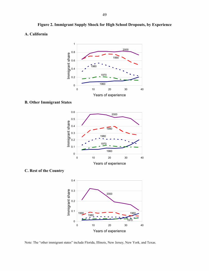
49

Figure 2. Immigrant Supply Shock for High School Dropouts, by Experience

A. California

B. Other Immigrant States

C. Rest of the Country

Note: The “other immigrant states” include Florida, Illinois, New Jersey, New York, and Texas.

0

0.2

0.4

0.6

0.8

1

0 10 20 30 40

Years of experience

1960

1970

1980

1990

2000

Imm

igra

nt s

hare

0

0.1

0.2

0.3

0.4

0.5

0.6

0 10 20 30 40

Years of experience

1960

1970

1980

1990

2000

Imm

igra

nt s

hare

0

0.1

0.2

0.3

0.4

0 10 20 30 40

Years of experience

1960

1970

19801990

2000

Imm

igra

nt s

hare

50

Figure 3. Immigrant Supply Shock for College Graduates, By Experience

A. California

B. Other Immigrant States

C. Rest of the Country

Note: The “other immigrant states” include Florida, Illinois, New Jersey, New York, and Texas.

0

0.1

0.2

0.3

0.4

0 10 20 30 40

Years of experience

19601970

1980

1990

2000

Imm

igra

nt s

hare

0

0.05

0.1

0.15

0.2

0.25

0 10 20 30 40

Years of experience

1960

1970

1980

1990

2000

Imm

igra

nt s

hare

0

0.03

0.06

0.09

0.12

0 10 20 30 40

Years of experience

1960

1970

1980

1990

2000

Imm

igra

nt s

hare

51

Figure 4. Geographic Sorting of Native Population and Immigration

A. California

B. Other Immigrant States

C. Rest of the Country

Note: The “other immigrant states” include Florida, Illinois, New Jersey, New York, and Texas.

6.0%

7.0%

8.0%

9.0%

10.0%

1950 1960 1970 1980 1990 2000

Year

Perc

ent o

f nat

ives

liv

ing

in r

egio

n

6.0%

14.0%

22.0%

30.0%

38.0%

Imm

igra

nt s

hareNative trend

Immigration

23.5%

24.5%

25.5%

26.5%

1950 1960 1970 1980 1990 2000

Year

Perc

ent o

f nat

ives

liv

ing

in r

egio

n

6.0%

12.0%

18.0%

24.0%

Imm

igra

nt s

hare

Native trend

Immigration

64.0%

65.0%

66.0%

67.0%

1950 1960 1970 1980 1990 2000

Year

Perc

ent o

f nat

ives

liv

ing

in r

egio

n

0.0%

4.0%

8.0%

12.0%

16.0%

Imm

igra

nt s

hare

Native trend

Immigration

52

Figure 5. Scatter Diagram Relating the Growth Rate of the Native Workforce and Immigration

A. State Level Data

B. Metropolitan area level data

Notes: Each data point represents the decadal change (between 1960 and 2000 in the top panel; between 1980 and 2000 in the bottom panel) observed in the log size of the native workforce and the change in the immigrant share for a particular skill group in a particular geographic area. Both plots remove decade effects from the data.

53

Table 1. Trends in inter-region migration rates of native workers Year Education group Region 1970 1980 1990 2000 Net migration rates

High school dropouts California -0.2% -2.2% -2.3% -5.4% Other immigrant states 0.3 -0.2 -1.6 -1.4 Rest of country -0.1 0.3 0.8 1.0 High school graduates California 0.3 -1.4 -0.8 -4.5 Other immigrant states 0.0 -0.1 -0.8 -0.9 Rest of country 0.0 0.2 0.4 0.7 Some college California 1.3 -1.0 0.3 -3.4 Other immigrant states -0.4 -0.3 -0.9 -0.8 Rest of country -0.2 0.4 0.3 0.9 College graduates California 4.4 3.3 4.5 1.9

Other immigrant states 0.3 -0.3 -0.8 -0.4 Rest of country -1.0 -0.4 -0.5 -0.1 In-migration rates

High school dropouts California 7.6 6.9 6.2 4.0 Other immigrant states 3.8 4.7 4.5 4.2 Rest of country 1.8 2.3 2.6 2.5 High school graduates California 8.7 8.3 7.7 4.9 Other immigrant states 5.4 6.0 5.2 4.6 Rest of country 2.7 2.8 2.6 2.5 Some college California 8.6 8.8 7.9 5.3 Other immigrant states 7.0 8.1 6.8 6.2 Rest of country 4.4 4.8 4.0 3.6 College graduates California 14.3 14.1 13.0 11.1 Other immigrant states 11.9 11.9 10.0 9.4

Rest of country 6.2 6.3 5.4 4.8 Out-migration rates

High school dropouts California 7.8 9.1 8.5 9.5 Other immigrant states 3.6 4.9 6.1 5.6 Rest of country 1.8 2.0 1.9 1.6 High school graduates California 8.3 9.7 8.5 9.5 Other immigrant states 5.4 6.1 6.0 5.5 Rest of country 2.7 2.6 2.3 1.7 Some college California 7.3 9.8 7.5 8.7 Other immigrant states 7.4 8.4 7.7 7.0 Rest of country 4.6 4.4 3.7 2.8 College graduates California 9.9 10.8 8.4 9.2

Other immigrant states 11.7 12.1 10.8 9.8 Rest of country 7.2 6.7 5.9 4.9 Notes: This table breaks up the country into three distinct regions, California, the other immigrant states, and the rest of the country. The “other immigrant states” include Florida, Illinois, New Jersey, New York, and Texas. A native worker is defined to migrate if he moves from one of these regions to another in the five-year period prior to the Census.

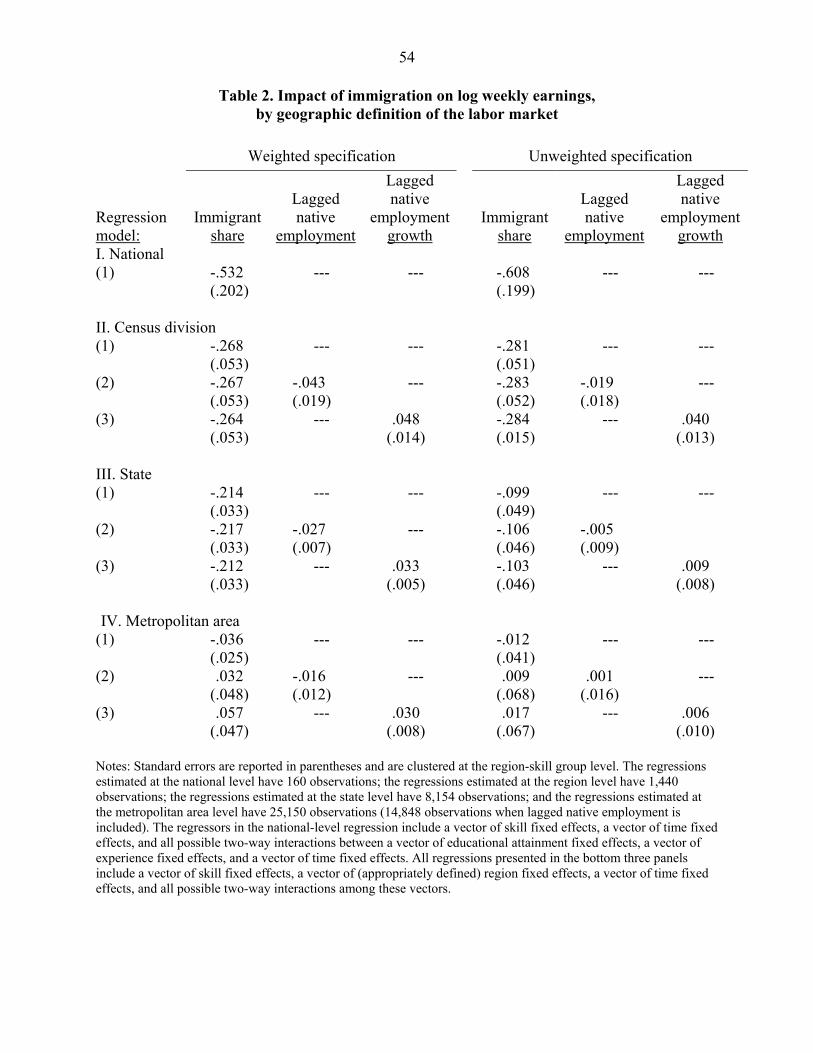
54

Table 2. Impact of immigration on log weekly earnings, by geographic definition of the labor market

Weighted specification Unweighted specification Regression model:

Immigrant share

Lagged native

employment

Lagged native

employment growth

Immigrant share

Lagged native

employment

Lagged native

employment growth

I. National (1) -.532 --- --- -.608 --- --- (.202) (.199) II. Census division (1) -.268 --- --- -.281 --- --- (.053) (.051) (2) -.267 -.043 --- -.283 -.019 --- (.053) (.019) (.052) (.018) (3) -.264 --- .048 -.284 --- .040 (.053) (.014) (.015) (.013) III. State (1) -.214 --- --- -.099 --- --- (.033) (.049) (2) -.217 -.027 --- -.106 -.005 (.033) (.007) (.046) (.009) (3) -.212 --- .033 -.103 --- .009 (.033) (.005) (.046) (.008) IV. Metropolitan area

(1) -.036 --- --- -.012 --- --- (.025) (.041) (2) .032 -.016 --- .009 .001 --- (.048) (.012) (.068) (.016) (3) .057 --- .030 .017 --- .006 (.047) (.008) (.067) (.010) Notes: Standard errors are reported in parentheses and are clustered at the region-skill group level. The regressions estimated at the national level have 160 observations; the regressions estimated at the region level have 1,440 observations; the regressions estimated at the state level have 8,154 observations; and the regressions estimated at the metropolitan area level have 25,150 observations (14,848 observations when lagged native employment is included). The regressors in the national-level regression include a vector of skill fixed effects, a vector of time fixed effects, and all possible two-way interactions between a vector of educational attainment fixed effects, a vector of experience fixed effects, and a vector of time fixed effects. All regressions presented in the bottom three panels include a vector of skill fixed effects, a vector of (appropriately defined) region fixed effects, a vector of time fixed effects, and all possible two-way interactions among these vectors.

55

Table 3. Impact of Immigration on the Size of the Native Workforce

(Dependent variable = Log of Number of Natives in Labor Force) Independent variables

Geographic area and specification

Immigrant share

Lagged native

employment

Lagged native

employment growth

Mean log wage

Unemployment rate

I. Census divisions (1) -.016 --- --- --- --- (.158) (2) .058 .244 --- .172 -1.342 (.121) (.042) (.115) (.439) (3) .143 --- .096 .263 -1.509

(.145) (.031) (.157) (.531) II. State

(1) -.376 --- --- --- --- (.093) (2) -.278 .056 --- .020 -.388 (.081) (.015) (.048) (.195) (3) -.269 --- .038 .117 -.649

(.085) (.011) (.056) (.211) III. Metropolitan area

(1) -.781 --- --- --- --- (.060) (2) -.836 -.403 --- .075 -.303

(.090) (.023) (.044) (.154) Notes: Standard errors are reported in parentheses and are clustered at the region-skill group level. The regressions estimated at the region level have 1,440 observations (1,152 observations when the lagged native employment growth is included); regressions estimated at the state level have 8,158 observations (6,434 observations when the lagged native employment growth is included); and the regressions estimated at the metropolitan area level have 25,151 observations (14,848 observations when the lagged native employment is included). All regressions include a vector of skill fixed effects, a vector of (appropriately defined) region fixed effects, a vector of time fixed effects, and all possible two-way interactions among these vectors.

56

Table 4. Impact of Immigration on Native Migration Rates

Independent variables

Geographic area and dependent variable

Immigrant share

Lagged native

employment growth

Lagged native

employment Mean log

wage Unemployment

rate I. Census division

1. Net migration rate -.076 .061 --- .150 -.035 (.046) (.023) (.056) (.207) 2. Net migration rate -..066 --- .050 .164 -.117 (.042) (.023) (.057) (.200) 3. In-migration rate -.102 -.015 --- .113 .159 (.034) (.010) (.040) (.143) 4. Out-migration rate -.027 -.076 --- -.037 .194

(.033) (.018) (.041) (.166) II. State

1. Net migration rate -.282 -.018 --- .010 .270 (.064) (.014) (.070) (.211) 2. Net migration rate -.288 --- -.067 .013 .310 (.064) (.018) (.069) (.209) 3. In-migration rate -.150 -.054 --- .020 .042 (.042) (.009) (.035) (.126) 4. Out-migration rate .132 -.035 --- .010 -.228

(.049) (.013) (.052) (.170) III. Metropolitan area

1. Net migration rate -.404 -.089 --- -.045 .046 (.084) (.014) (.041) (.140) 2. Net migration rate -.289 --- -.065 -.068 .081 (.086) (.020) (.041) (.140) 3. In-migration rate -.116 -.076 --- -.015 .032 (.055) (.009) (.027) (.094) 4. Out-migration rate .288 .012 --- .030 -.014

(.062) (.010) (.028) (.097) Notes: Standard errors are reported in parentheses and are clustered at the region-skill group level. The regressions estimated at the region level have 1,152 observations; the regressions estimated at the state level have 6,524 observations; and the regressions estimated at the metropolitan area level have 14,847 observations. All regressions include a vector of skill fixed effects, a vector of (appropriately defined) region fixed effects, a vector of time fixed effects, and all possible two-way interactions among these vectors.

57

Table 5. Sensitivity of Results

(Coefficient of immigrant share variable in state-level regressions)

Specification

Log (Native

Workforce)Migration Regressions

Net migration In-migration Out-migration 1. Baseline (Men) -.278 -.282 -.150 .132 (.081) (.064) (.042) (.049) 2. Men outside California -.313 -.299 -.148 .151 (.086) (.069) (.045) (.052) 3. Men with at least a high -.820 -.279 -.248 .031

school degree (.176) (.218) (.123) (.158) 4. Men, but includes women -.228 -.268 -.127 .141

in counts of workers (.086) (.071) (.046) (.053) 5. Women -.360 -.166 -.048 .118 (.102) (.073) (.048) (.054) 6. Men and women -.298 -.232 -.100 .132 (.082) (.057) (.036) (.039) Notes: Standard errors reported in parentheses; all standard errors are clustered by skill and region. The baseline male regressions on the log of the native workforce have 8,158 observations (6,524 observations in the migration regressions); the non-California regressions have 7,903 observations (6,396); the regressions for workers with at least a high school education have 6,039 observations (4,892); the regressions estimated in the sample of women have 8,030 observations (6,526); and the regressions in the sample of all workers have 8,083 observations (6,528). The regressions include a vector of skill fixed effects, a vector of (appropriately defined) region fixed effects, a vector of time fixed effects, all possible two-way interactions among these vectors, and the mean log weekly wage and unemployment rate in the labor market. In addition, the regressions on the native workforce include the lagged value of the log of the native workforce, while the migration regressions include the lagged value of the growth rate of the native workforce.

58

Table 6. Synthesis of Wage and Migration Effects Census

division State Metropolitan area

1. Estimate of factor price elasticity (in national -.372 -.372 -.372 labor market)

2. Estimate of migration effect:

Simple specification: native workforce -.011 -.263 -.547 Complete specification: native workforce .041 -.195 -.585 Complete specification: net migration -.053 -.197 -.283

3. Predicted estimate of spatial correlation:

Simple specification: native workforce -.367 -.274 -.169 Complete specification: native workforce --- -.299 -.154 Complete specification: net migration -.352 -.299 -.270

4. Spatial correlation actually estimated at local level:

Simple specification -.188 -.150 -.025 Complete specification -.187 -.152 .022

Notes: The synthesis is based on the theory-based interpretation of the coefficients reported in Tables 2, 3, and 4. See the text for details.