Internal Borders and Migration in India∗

Zovanga L. Konea,b, Maggie Y. Liua,c, Aaditya Mattooa, Caglar Ozdena and Siddharth Sharmaa

aWorld Bank Group

bUniversity of Nottingham

cGeorgetown University

September 2016

Abstract

Internal mobility is a critical component of economic growth and development as itenables the reallocation of labor to more productive opportunities across sectors andregions. Using detailed district-to-district migration data from the 2001 Census of India,we highlight the role of the state borders as significant impediments to internal mobility.We find that average migration between neighboring districts in the same state is atleast 50 percent larger than neighboring districts on different sides of a state border evenafter accounting for linguistic differences. While the impact of state borders differs byeducation, age and reason for migration, it is always large and significant. We suggestthat inter-state mobility is inhibited by the existence of state level entitlement schemes,ranging from access to subsidized goods through the public distribution system to the biasfor states’ own residents in access to tertiary education and public sector employment.

Keywords: Internal migration; internal borders; immigration; emigrationJEL codes: J6; O15; F22

∗We would like to thank the Data Dissemination Unit, Office of the Registrar General and Census Commis-sioner of India for preparing the data tables from the 2001 Census under a special administrative agreementwith the World Bank. We are also grateful to Erhan Artuc, Simone Bertoli, Bernard Hoekman, Chris Parsons,Mathis Wagner and participants at the 9th International Migration and Development Conference (June 2016)in Florence for comments, Professor Ravi Srivastava (JNU) for his valuable insights on internal migration inIndia, and Virgilio Galdo and Yue Li (Office of the Chief Economist, South Asia, World Bank) for sharing GISshapefiles of India’s districts. We acknowledge the financial support from the Knowledge for Change Program,the Multi-Donor Trust Fund for Trade and Development, and the Strategic Research Program of the WorldBank. The findings in this paper do not necessarily represent the views of the World Bank’s Board of ExecutiveDirectors or the governments they represent. Any errors or omissions are the authors’ responsibility.

1

1 Introduction

Development and economic growth take place through the more efficient allocation of inputs

into more productive uses. Labor is a key input since it is the main asset of the majority of

the population, especially of the poor, in developing countries. The reallocation of labor can

take place across sectors, occupations and, most importantly, geographic regions. Thus, it is no

surprise that every successful development experience and growth episode is accompanied by

large labor movements, especially from rural to urban areas, and from low to higher productivity

employment. In this regard, India presents a paradox and daunting challenge.

As of 2001, internal migrants represented 30 percent of India’s population. A closer inspection

of the data, however, reveals that two-thirds are intra-district migrants, more than half of whom

are women migrating for marriage. Even more striking, those who have migrated within the

last five years preceding 2001 account for less than 3 percent of the population. In contrast, in

the U.S., those who moved from one state to another within a given five-year period accounted

for 12 percent of the population in 2005 (Molloy et al, 2011). Moreover, in a cross national

comparison of internal migration rates over a five year interval between the years 2000 and

2010, Bell et al. (2015) show that India ranks last in a sample of 80 countries. The low level

of migration in India relative to other emerging economies is also reflected in the country’s

relatively low urbanization rate: 28 percent in 2000, 15 percent less than in countries with

comparable GNP levels (Anderson and Deshingkar, 2004).1

The paper makes several contributions. The first is the introduction of a very detailed district-

to-district census-based migration data disaggregated by age, education, duration of stay and

reason for migration. Most existing studies in India use survey data that suffer from sampling

and aggregation biases and are rarely bilateral. Our data allow us to control for origin and

destination specific factors (such as natural endowments, economic and social conditions, and

climate) through fixed effects. Thus, we are able to focus on bilateral variables as the gravity

1The urbanization rate increased only marginally to 31 percent in 2011 (Sharma and Chandrasekhar, 2014).

2

literature emphasizes. Among these are the critical contiguity variables – being in the same

state and/or being geographic neighbors – in addition to the standard geographic distance

and linguistic overlap measures. In addition, by using data from 585 districts to 585 districts,

instead of the standard state-to-state analysis in other papers, we are able to solve many of

the aggregation problems that arise in large countries like India. For example, Uttar Pradesh

would rank as the fifth most populous country in the world if it were independent, and treating

it as a single observation creates many biases.

The second and more substantive contribution is to demonstrate the role played by administra-

tive barriers, particularly in the form of state borders, in limiting internal migration in India.

Our empirical analysis shows that, even when we control for numerous barriers to internal mo-

bility, such as physical distance, linguistic differences and all economic and social barriers in

origin and destination districts (through district fixed effects), state borders continue to impose

important impediments. Migration between neighboring districts in the same state is at least

50 percent larger than migration between districts which are on different sides of a state bor-

der. This gap varies by education level, age and reason for migration, but is always large and

significant. The creation of three new states in November 2000 provides a natural experiment

and additional evidence. We find that these new state borders are not natural barriers but

administrative restrictions on internal mobility.

The low level of internal mobility in India – including the role of state borders – cannot be

attributed directly to restrictive federal government policies. This is unlike some other countries

where the role of government policies in influencing internal migration patterns has been noted.

For example, federal government policies have constrained migration through measures such

as the hukou system in China. There are, however, no such measures in India, and anyone

is legally free to move from one district to another. In principle, federal laws protect migrant

workers, especially from exploitation in destination regions. One such provision is the Inter

State Migrant Workmen Act, 1979, which requires that migrants are paid timely wages equal

3

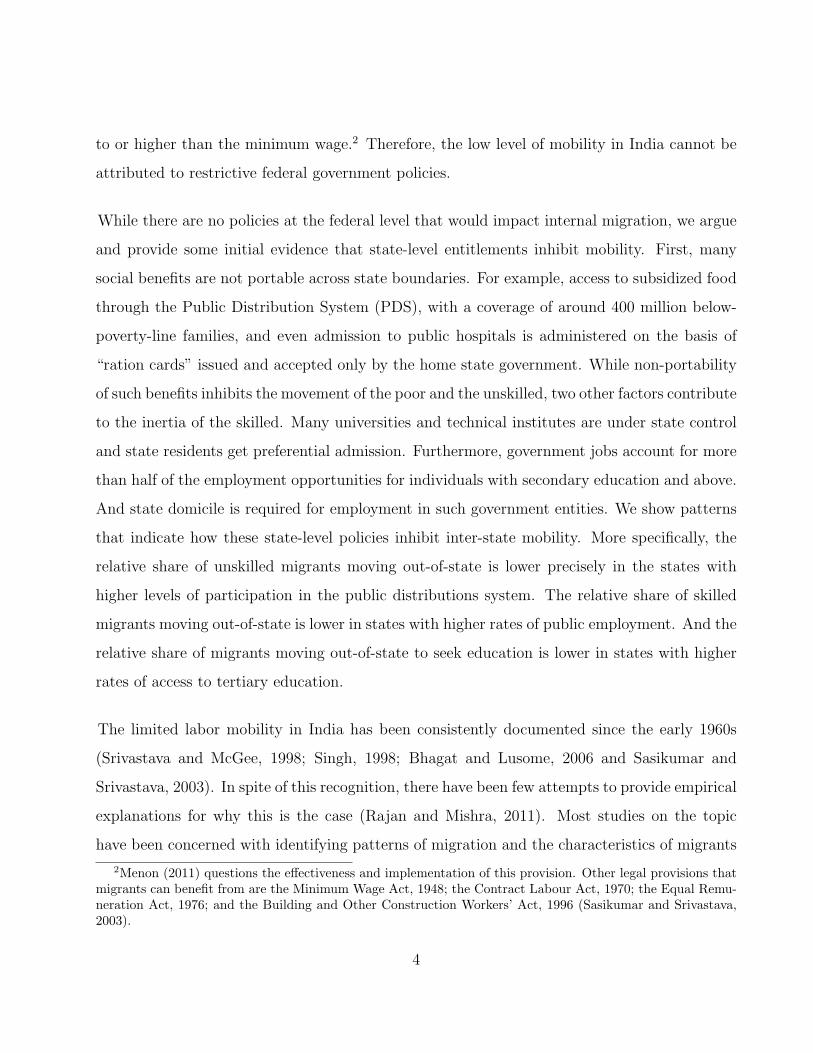
to or higher than the minimum wage.2 Therefore, the low level of mobility in India cannot be

attributed to restrictive federal government policies.

While there are no policies at the federal level that would impact internal migration, we argue

and provide some initial evidence that state-level entitlements inhibit mobility. First, many

social benefits are not portable across state boundaries. For example, access to subsidized food

through the Public Distribution System (PDS), with a coverage of around 400 million below-

poverty-line families, and even admission to public hospitals is administered on the basis of

“ration cards” issued and accepted only by the home state government. While non-portability

of such benefits inhibits the movement of the poor and the unskilled, two other factors contribute

to the inertia of the skilled. Many universities and technical institutes are under state control

and state residents get preferential admission. Furthermore, government jobs account for more

than half of the employment opportunities for individuals with secondary education and above.

And state domicile is required for employment in such government entities. We show patterns

that indicate how these state-level policies inhibit inter-state mobility. More specifically, the

relative share of unskilled migrants moving out-of-state is lower precisely in the states with

higher levels of participation in the public distributions system. The relative share of skilled

migrants moving out-of-state is lower in states with higher rates of public employment. And the

relative share of migrants moving out-of-state to seek education is lower in states with higher

rates of access to tertiary education.

The limited labor mobility in India has been consistently documented since the early 1960s

(Srivastava and McGee, 1998; Singh, 1998; Bhagat and Lusome, 2006 and Sasikumar and

Srivastava, 2003). In spite of this recognition, there have been few attempts to provide empirical

explanations for why this is the case (Rajan and Mishra, 2011). Most studies on the topic

have been concerned with identifying patterns of migration and the characteristics of migrants

2Menon (2011) questions the effectiveness and implementation of this provision. Other legal provisions thatmigrants can benefit from are the Minimum Wage Act, 1948; the Contract Labour Act, 1970; the Equal Remu-neration Act, 1976; and the Building and Other Construction Workers’ Act, 1996 (Sasikumar and Srivastava,2003).

4

(Singh, 1998; Bhagat and Lusome, 2006; Hnatkovska and Lahiri, 2015). In a more recent

study, Arvind Pandley (2014) for instance documents a slight upward trend in the overall level

of migration from the early 1990s, primarily driven by increased intra-district and intra-state

movements. These upward trends are attributed to economic reforms in the 1990s that boosted

the development of large cities through government subsidies for industrial and infrastructure

development in various states, which attracted professionals and entrepreneurs.

Munshi and Rosenzweig (2016), Bhattacharyya (1983) and Viswanathan and Kumar (2015)

are exceptions that move beyond descriptive analyses. While the last paper examines how

migration responds to environmental changes, the first two papers provide an explanation for

the low levels of rural to urban migration in India. Bhattacharyya (1983) presents a theoretical

framework for developing countries, in which the migration decisions are less likely to be taken at

the individual level than at the (extended) family level. Whereas the individual decision would

be mostly driven by wage differentials between the destination and the origin labor markets,

a family would decide who and how many members should migrate in order to increase the

overall income/output level of the family. Closely related, Munshi and Rosenzweig (2016) posit

that the caste network in rural areas creates an impediment to rural to urban migration by

providing insurance for low-income households in their communities as well as for households

facing income fluctuations. They provide a theoretical explanation and empirical evidence that

we observe low levels of migration among the least wealthy in the community because the

migration of an individual (often an income earner) reduces access to caste networks for the

family members who are left behind. While this explanation is consistent with the case of rural

to urban migration, where community networks exert strong influence on the decisions of its

members in rural areas, it may not explain why urban to urban migration is also low or why

we observe differences in migration patterns across state borders.

In general, moving across certain boundaries is costly, especially if these boundaries reflect

differences in societal characteristics such as cultures, laws and institutions (Belot and Ed-

5

erveen, 2012). The first study to point out such a cost was by McCallum (1995) in the field

of trade. McCallum showed that Canadian provinces adjacent to the United States undertook

much higher levels of trades with their neighboring provinces than with the U.S. A number of

subsequent studies have corroborated McCallum’s findings and unearthed evidence of a border

cost in the case of migration (Helliwel, 1997; and Poncet, 2006). Helliwel (1997) in particular

suggest that inter-provincial migration in Canadian provinces is almost 100 times as likely as

migration to Canadian provinces from the United States, Canada’s closest neighbor. But these

studies do not explore the role of internal borders.

Migration costs naturally impede internal migration flows in a country. Bayer and Juessen

(2012) suggest that inter-state migration in the U.S. can cost the migrant up to two-thirds of

an average American’s household annual income. In her study of internal migration in China,

Poncet (2006) examines determinants of rural to urban migration in China, focusing on the

role of contiguity, distance, provincial borders and wage levels at the destination. The findings

suggest migration flows between two localities are negatively related to distance but positively

related to contiguity (as well as with wage levels at the destination). More relevant to our

paper, they too find that there is more intra-province migration in comparison to inter-province

migration.

The next section presents the internal migration data, the geographic and linguistic distance

variables as well as several empirical observations that motivate the analysis. Section 3 intro-

duces the gravity model and our empirical specification. We then discuss the results and end

with the conclusions.

6

2 Data

2.1 Data source and empirical observations

The main data source in this paper is the National Census of India for 2001.3 The census

has been conducted every decade since 1871 and the responsibility currently rests with the

Office of the Registrar General and Census Commissioner under the Ministry of Home Affairs.

The national census, like those in many other countries, collects individual and household level

information on various demographic and labor market characteristics for the whole popula-

tion. We supplement the census with additional household and labor force data from the 55th

Round of the National Sample Survey (NSS) from 1999-2000. The NSS, covering over 100

thousand households, is administered by the Ministry of Statistics and is conducted annually.

In addition to standard household modules on consumption, health, education, employment

and investment, it includes specialized surveys that rotate each year. The NSS includes a more

detailed set of questions in comparison to the Census and therefore, provides more detailed

data, but for a much smaller sample of the population.

The census asks two different questions pertaining to the migration status of the respondents,

leading to two different definitions as to who can be considered a migrant. The first question

is on the place of birth of the individual, the standard criteria in many surveys and censuses

(Carletto et al. 2014). Migrants are defined as “those who are enumerated at a village/town

at the time of census other than their place of birth.” The second question focuses on the

place of last residence, instead of birthplace. An individual is defined as a migrant “if the

place in which he is enumerated during the census is other than his place of immediate last

residence” (Census, 2001). We choose the residence-based definition to identify migrants in our

analysis for two reasons. First, additional questions are asked if the individual is classified as

a migrant based on this criteria; this is not the case with the birthplace classification. These

3As of the date of drafting of this paper, the migration related portions of the 2011 Census have not beenprocessed.

7

additional questions include reason of migration (marriage, education, employment etc.), the

urban/rural status of the location of last residence and the duration of stay in the current

residence since migration. The answers to these questions shed additional light on the patterns

and determinants of internal mobility. Second, while less commonly available in other datasets,

this criteria is more relevant in economic analysis of internal mobility patterns.

While the census questionnaire asks these questions to each respondent, the resulting individual

level data are not made publicly available. Instead, the data are aggregated up to geographic

units – depending on the purpose – and are disseminated through tables at these geographic

aggregation levels. For example, we can find the number of people living in a given district

whose previous residence was in a different state or another district within the same state. In

some cases, the tables published by the Census include additional variables, such as gender,

education or reason for migration. However, none of these datasets present bilateral migrant

stocks at the district level.

The publicly available tables do not lend themselves to empirical analysis, especially to gravity

type estimation. Therefore, we approached the Census Bureau with a specific request for

detailed bilateral (district-to-district) migration data. Since they could not release individual

or household level data, the Census Bureau constructed a series of bilateral tables under a

special administrative agreement. These tables contained the following for all pairs of districts

in India: 1) migration stocks by gender and educational attainment levels, 2) migration stocks

by gender and age groups, 3) migration stocks by gender and reason for migrating, and 4)

migration stocks by gender and duration of stay at the destination. All data are at the district

level, including within-district migration stocks as well as non-migrant stocks. Each of these

tables have over 350 thousand rows and between 10 and 16 columns.4

4The 2001 administrative division of India has 593 districts, 9 of which are districts in Delhi. In our analysis,we combined the nine districts in Delhi, and treat Delhi as one single district. This leaves us with 585 districtsin our empirical analysis.

8

The data tables from the Census Bureau allow us to distinguish four subgroups of the popula-

tion: 1) non-migrants, 2) intra-district migrants, i.e. those who moved from one enumeration

area to another one within the same district, 3) inter-district migrants within the same state,

i.e. those who moved across districts within the same state, and 4) inter-state migrants, i.e.

those who moved across states. Table 1 presents the sizes of these groups by gender. Migrants

account for close to 30 percent of the population in 2001, albeit with considerable divergence in

patterns across genders. The share of migrants among females (43.3 percent) is three times the

share of migrants among males (16.3 percent). This big gap is due to the well-known migra-

tion of women to nearby areas within the same or neighboring districts for marriage reasons.

The share of intra-district migrants among women is 29.5 percent, over three times the level

among men. Inter-district (but intra-state) migration among women is 9.8 percent, over twice

the level among men. Finally, inter-state migration among women is 4 percent, slightly higher

than among men.

The low level of internal migration in India and the gender gaps are are further illustrated by

Figures 2 to 5 where we present migration rates at destination and origin by gender for each

district. The maps cover 585 districts across 35 states and union territories. In each map,

state boundaries are outlined with thick lines, and districts are color-coded in gradients of blue,

where darker-shaded districts have relatively higher shares of the relevant migration measure.

We see clear variation in the migration levels across different areas of India.

Figure 2 plots the share of all inter-district migrants (the sum of intra-state-inter-district mi-

grants and inter-state migrants, groups 3 and 4 from the earlier discussion) among the existing

population in each district in India. The map on the right is much “darker” in color, indicating

the higher level of inter-district migration among women. In 337 districts, over ten percent of

the current female migrants are inter-district migrants, while only 101 districts have the same

share among male population. Furthermore, we observe more migration to the West coast, es-

pecially to districts in Maharashtra, and to Northwestern states, especially to Punjab, Haryana

9

and Delhi. Figure 3 plots the share of inter-district emigrants among population from origin

districts, i.e. out-migration. Similarly, on average, more women migrate to other districts. The

median level of emigration is 4.4 percent for men and 10 percent for women. Emigration is

concentrated in the North and West, mainly in Uttar Pradesh, West Bengal and Maharashtra.

The data allow us to further differentiate between migrants who move across district borders.

More specifically, we can compare those who stay within the same state (intra-state migrants)

with those who move to another state (inter-state migrants). Figure 4 and 5 present the size

of inter-state migrants relative to all inter-district migrants in destination and origin districts,

respectively. Even though the number of female migrants far exceeds that of male migrants,

female migration is mostly within the same state while male migrants are more likely to cross

state borders. That is why the map on the left (for men) is darker in color than the map on the

right. On average, 43 percent of male migrants are from another state, compared to 29 percent

of female inter-district migrants. When we compare Figures 4 and 5, we see that inter-state

emigration, especially for men, is more concentrated in the Northern states of Uttar Pradesh,

Bihar and Rajasthan. Furthermore, districts that receive (send) higher shares of migrants from

(to) other states are located along state borders, an issue which we will explore in detail in the

empirical section.

The key feature of our dataset is its bilateral nature at the district level. To highlight this and

the role of the state borders on internal migration, we take the district of Nagpur in Maharashtra

as an example. We chose Nagpur since it is geographically located at the center of India and

close to three other states – Andra Pradesh, Madhya Pradesh and Chattisgarh. Figure 6 plots

the distribution of the origin districts of the migrants coming to Nagpur. All origin districts

are colored in different shades of blue according to the share of in-migrants in Nagpur from

that district. The vast majority of the migrants come from districts that are in the same state

or in neighboring states to Nagpur. In fact, four out of the top five sending districts are in

Maharashtra, and six out of the seven districts that share a border with Nagpur are among the

10

top ten senders. The four neighboring districts in Maharashtra (Bhandara, Wardha, Amravati,

and Chandrapur) send a total of 31 percent of Nagpur’s immigrants. The remaining three

neighboring districts in Madhya Pradesh (Balaghat, Chhindwara, and Seoni) send a total of

13 percent. The prohibitive role of state borders becomes more clear when we note there

are more migrants from distant districts in Maharashtra than from nearby districts in other

states. In Figure 7, similar patterns are observed when we look at migration from Nagpur to

other districts. The most popular destinations of Nagpur’s emigrants are neighboring districts

in Maharashtra (Bhandara, Wardha, Amravati, and Chandrapur) which receive a total of 32

percent migrants from Nagpur. The neighboring districts in other states receive smaller shares

of emigrants. Nearby districts in other states receive much fewer migrants when compared to

distant coastal districts of Maharashtra as seen in Figure 7(a).

As mentioned earlier, the tables from the Census Bureau have the bilateral migration data

disaggregated by other variables. The first disaggregation is by age groups and the data are

presented in Table 2 by gender. The share of migrants are highest among those between 25

and 65 years of age. This is especially stark for women where the migrant ratio dramatically

increases from 23.2 percent (for 14-19 year olds) to 69.1 percent (for the 25-34 year olds),

highlighting the role of marriage in migration. The corresponding increase is much less drastic

among men. Non-migrants account for the largest share among men, followed by intra-district

migrants, inter-district migrants within the same state and inter-state migrants. Furthermore,

males in the 25-65 age groups, i.e. prime working age, show similarly low migration levels.

The next variable of interest is the migration status across educational attainment groups.

Table 3 illustrates patterns of migration for four education levels by gender: (i) illiterate, (ii)

primary school education, (iii) secondary school education, and (iv) tertiary education. An

immediate observation is that those with higher educational levels appear to be more mobile.

This holds for both aggregate levels of migration as well as for movements across geographical

boundaries. For instance, migrants account for 35.6 percent of the tertiary educated male pop-

11

ulation compared with 11.5 percent for the illiterate male population, and inter-state migrants

represent 8.4 percent among the former but only 2.1 among the latter. Turning to the female

population on the second half of the table, we see the same patterns. Inter-district migrants

within the state account for the largest proportion of migrants among the tertiary educated,

suggesting that distance or geographical boundaries are less constraining for them relative to

other education groups.

The reason for migration is one of the most important questions in the census questionnaire.

We aggregated the answers into five main categories: (i) work or business, (ii) marriage, (iii)

move with the family, (iv) education, and (v) other reasons. For men, work/business, move with

the family and others are the main reasons (around 30 percent each) while marriage dominates

all other categories for women (70 percent). Unfortunately, the format of the data do not allow

us to construct cross-tabulations, such as by education and reason for migration, which would

provide further insights.

Closely linked to the flexibility of moving across geographical boundaries is the duration of stay

at the destination. Table 5 reports summary statistics on the origin distribution of migrants

across four intervals of duration of stay at their destinations. The data suggests that most

migrants (i.e. about 50 percent) have lived at their host destination for over 10 years, although

this is driven by females migrants. Regardless of the duration of stay considered, there is very

little variation in the distribution of migrants by origin (e.g. inter-state versus intra-state),

specially among males. This reinforces the observation made in the previous section that low

internal mobility in India is possibly due to mobility costs across geographical and institutional

boundaries.

2.2 Migration Measures and Other Controls

The data used in the empirical analysis are based on the migration data described above. In

addition, we construct several explanatory variables needed for the gravity estimation. These

12

are standard bilateral distance, linguistic overlap and other geographic proximity variables.

They are described and discussed in detail below.

Bilateral Migration Stocks

We define mij as the stock of migrants who moved from origin (or previous) district i to

destination (or current) district j as of 2001.5 In the previous section, we had also identified

intra-district migrants as people who moved within a district. In the empirical analysis, we

ignore this group and add them to non-migrants. We disaggregate the migrant numbers also

by education, age, reason of migration and duration as we proceed and mij will accordingly

represent the relevant bilateral migrant stock.

Following the approach in gravity models of international migration, we control for dyadic

factors that influence migration costs: physical distance, linguistic proximity,6 contiguity, and

state borders.7 The construction of these control variables are explained below.

State Borders and Contiguity

Since the seminal work of McCallum (1995) on the importance of the Canada-U.S. border on

international and intra-national bilateral trade volumes, borders have been at the center of

analysis of trade patterns. The argument extends to migration: borders, either physical or

institutional, could impose costs on mobility. Unlike the international trade literature which

extensively documents the striking large effect of national borders on trade,8 few studies have

empirically tested the border effect on internal migration.9 One explanation is the lack of

region-to-region migration data in different countries. The district level data used in this paper

overcome this hurdle and provide a unique opportunity to compare intra-state vs. inter-state

5Since we only measure the migrant stock at 2001, we do not observe return or circular migration.6We are working to include cultural proximity and network variables using religion and caste information.7We should note that origin and destination specific factors are not included since we control for them with

origin and destination fixed effects in our empirical analysis.8See Anderson and van Wincoop (2001, 2004) for extensive reviews9One exception is Helliwel (1997), which found interprovincial migration among the Canadian provinces is

much larger than US states-Canada province migration. Although the data used in Helliwel (1997) does notinclude bilateral U.S. state- Canadian province migration data.

13

migration in India, and thus examine the state border effect.

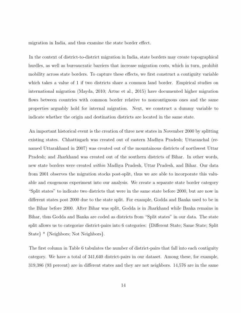
In the context of district-to-district migration in India, state borders may create topographical

hurdles, as well as bureaucratic barriers that increase migration costs, which in turn, prohibit

mobility across state borders. To capture these effects, we first construct a contiguity variable

which takes a value of 1 if two districts share a common land border. Empirical studies on

international migration (Mayda, 2010; Artuc et al., 2015) have documented higher migration

flows between countries with common border relative to noncontiguous ones and the same

properties arguably hold for internal migration. Next, we construct a dummy variable to

indicate whether the origin and destination districts are located in the same state.

An important historical event is the creation of three new states in November 2000 by splitting

existing states. Chhattisgarh was created out of eastern Madhya Pradesh; Uttaranchal (re-

named Uttarakhand in 2007) was created out of the mountainous districts of northwest Uttar

Pradesh; and Jharkhand was created out of the southern districts of Bihar. In other words,

new state borders were created within Madhya Pradesh, Uttar Pradesh, and Bihar. Our data

from 2001 observes the migration stocks post-split, thus we are able to incorporate this valu-

able and exogenous experiment into our analysis. We create a separate state border category

“Split states” to indicate two districts that were in the same state before 2000, but are now in

different states post 2000 due to the state split. For example, Godda and Banka used to be in

the Bihar before 2000. After Bihar was split, Godda is in Jharkhand while Banka remains in

Bihar, thus Godda and Banka are coded as districts from “Split states” in our data. The state

split allows us to categorize district-pairs into 6 categories: {Different State; Same State; Split

State} * {Neighbors; Not Neighbors}.

The first column in Table 6 tabulates the number of district-pairs that fall into each contiguity

category. We have a total of 341,640 district-pairs in our dataset. Among these, for example,

319,386 (93 percent) are in different states and they are not neighbors. 14,576 are in the same

14

state and not neighbors etc.

Distance

The physical distance between two districts is expected to strongly affect transportation costs

and, hence, migration levels. More distant districts would require higher monetary costs to

travel. At the same time, the uncertainty on earnings at the prospective destination is higher

because it is more difficult to acquire information ex-ante. For bilateral distance between

any two districts, we calculate geodetic distances – the length of the shortest curve between

two points along the surface of a mathematical model of the earth – between the districts’

geographical centers.10

Linguistic Proximity

Another important component of bilateral migration costs is the linguistic difference (Belot and

Ederveen, 2012; Adsera and Pytlikova, 2015). Linguistic proximity reduces migration costs by

lowering the cost of communication and skill transferability, especially for the less skilled.

First, we measure linguistic distance between any two districts (i, j) following the commonly

used ethnolinguistic fractionalization (EFL) index (Atlas Narodov Mira, 1964), which measures

the probability of two randomly chosen individuals from different groups speaking the same

language. We concentrate on mother tongue, which is “the language spoken in childhood by

the person’s mother to the person”, according to the 2001 Census of India. In addition to data

availability, we argue that there are two advantages in using the mother tongue. First, each

individual has a unique mother tongue even if they are multilingual. Second, mother tongue

relates more closely to an individual’s birth place, family background, and social networks. In

the 2001 Census of India, there are 122 categories of mother tongues, and all districts have

multiple mother tongues spoken by the observed population.

We construct two different measures of linguistic proximity between two districts: Common Languageij

and Language Overlapij. Let sli and slj be the share of individuals speaking mother tongue l

10We restrict centroids to be inside the boundaries of a polygon.

15

in districts i and j, respectively. Then sli ∗ slj is the probability that an individual from i

can speak to an individual from j in language l. Summing over all possible mother tongues,

Common Languageij measures the likelihood of any two individuals being able to communicate

in a common language. This is given by:

Common Languageij =∑l

sli · slj

Similarly, Language Overlapij measures the degree of overlap in languages spoken at any pair

of districts. min{sli, slj} is the intersection of people from each district who speak the same

language l. Since each person has only one mother tongue, summing over all possible mother

tongues, we have the overlap of people from two districts that can understand each other. This

is calculated as:

Language Overlapij =∑l

min {sli, slj}

Note that our linguistic proximity measures do not take into account the genealogical relations

(linguistic distance) between languages,11 and thus can be considered a lower bound of the

linguistic proximity across districts.

Table 6 summarizes the language and distance measures by contiguity of district-pairs. Overall,

neighboring districts are closer to each other in terms of distance and linguistic proximity

relative to non-neighboring districts. The average district-to-district log distance is 6.83. For

neighbors, regardless of whether they are in the same state or not, the log distance is 4.35,

which is 12 times smaller. In terms of linguistic proximity, several interesting patterns emerge.

First, districts that are in the same state have greater linguistic proximity than district-pairs

from two different states. This confirms linguistic distances were important in the drawing of

11Several studies use language trees from Ethnologue and use number of shared nodes between two languagesto construct a linguistic proximity measure. Such studies include Adsera and Pytlikova, 2015; Belot and Hatton,2012; Desmet et al., 2009; Desmet et al., 2012.

16

state borders. Second, districts from the split states are equally proximate in languages as

the same-state district-pairs, which suggests the 2000 state splits may have been less based on

language and ethnicity, relative to the original drawing of the original state borders. Third,

neighboring districts in different states have higher linguistic overlap than non-neighboring

districts in different states, but lower overlap compared with districts in the same state. In

other words, state borders are associated with discrete linguistic gaps but smaller than average

gaps.

3 Empirical Specification

In the empirical analysis to follow, we adopt a gravity specification, which is based on a random

utility maximization model. This specification has been extensively used in the analysis of

migration patterns.12 Our specification is given by:

(1) mij = α+β1·lnDISTij+β2·LANGij+γ1·DNBRij +γ2·DSTATE

ij +γ3·DNBRij ∗DSTATE

ij +δi+δj+ϵij

The dependent variable, mij, measures migration from origin i to destination j. In our case,

it is the level of inter-district migration stock. The bilateral independent variables introduced

previously are: lnDISTij, log geodesic distance between districts i and j; LANGij, linguistic

proximity between districts i and j; DNBRij , a dummy variable indicating whether districts i

and j share a common border, and DSTATEij , a categorical variable indicating whether districts

i and j are in the same state, from different states, or from split states. We interact DNBRij and

DSTATEij to investigate the additional impediments imposed by state borders.

Multilateral resistance, in the context of bilateral migration decisions, is the influence exerted

by the attractiveness of other destinations (Bertoli and Fernandez-Huertas Moraga, 2013),

and can introduce bias in the estimation if not properly addressed. We include origin and

12Beine et al., 2015; Beine and Parsons, 2015; Beine et al., 2011; Bertoli and Fernandez-Huertas Moraga,2013; Grogger and Hanson, 2011; Mayda, 2010.

17

destination fixed effects, δi and δj, to account for the multilateral resistance as well as for

unobserved heterogeneity in sending and receiving districts in our cross-sectional data.

We estimate the above specified gravity model using Poisson Pseudo-Maximum Likelihood, or

PPML (Santos Silva and Tenreyro, 2006). As thoroughly explained by Beine et al. (2015),

PPML is a more reliable estimator since, (1) OLS estimates are biased and inconsistent in the

presence of heteroskedasticity of ϵij, and (2) PPML performs well in the presence of a large

share of zeros, which is slightly over 40 percent of observations in our data.

In order to test whether the effect of bilateral migration hurdles changes over time, we later

explore the time dimension of our data by constructing a panel of migration flows based on

time of migration implied by duration of stay in destination districts. Following Bergstrand,

Larch and Yotov (2015), Equation (1) can be modified as follows:

(2)

mijt = α+β1·lnDISTijt+β2·LANGijt+γ1·DNBRijt +γ2·DSTATE

ijt +γ3·DNBRijt ∗DSTATE

ijt +δit+δjt+ϵijt

Here we construct time varying dyadic variables as the product of a year dummy Dt and time-

invariant dyadic variables xij. For example, LANGijt = Dt ·LANGij. Similarly, we control for

origin-time and destination-time fixed effects, δit and δjt.

4 Empirical Results

Our first set of results explore the determinants of aggregate migration and, more specifically

the role of district and state borders. As discussed earlier, the dependent variable is the

stock of migrants currently living in district j and whose previous residence was in district i.

Since we have fixed effects for both origin and destination districts, we include only bilateral

variables in the estimation – distance, language overlap and dummy variables for the contiguity

18

relationships. Each pair of districts can have one of the six possible relationships: (i) different

states and not neighbors, (ii) different states and neighbors, (iii) same state and not neighbors,

(iv) same state and neighbors, (v) split states and not neighbors and (vi) split states and

neighbors. In all of our estimations for the rest of the paper, the dummy variable for the first

group – different states and not neighbors – is dropped, and we include dummy variables for

each of the remaining five categories.

Table 7 presents the first set of gravity estimates. The first set of results – the first three

columns – is on total migration. The second set of results pertains to men and the final set is

on women. The first two columns in each set ignore the recently split states and assume they

were always separate states. The third column in each set introduces the recently split states

as we discussed above in the data section. Finally, the first and second columns in each set

have different linguistic overlap variables.

The distance variable has a negative coefficient in all specifications as expected and all estimates

are quantitatively close to each other. The language variables all have a positive sign, again

as expected, with higher coefficients for men, indicating language overlap is a more important

pull factor for them. The most important variables for our analysis are the contiguity dummy

variables. Since “Different states and not neighbors” is the default and dropped from the

regression, all other coefficients indicate the relative impact of a district border, state border

or being in the same state. We see that being in the same state and being neighbors increases

migration. For example, being in the same state but not neighbors increases migration (in

Column 1) by almost twice (e1.097 − 1). The impact of being in the same state is also higher

for men than women. Being in different states but neighbors also has a large positive effect.

In column 1, we see that total migration is around 4.5 times (e1.730 − 1) larger in this case and

this effect is stronger for women.

The most important observation is that the coefficient for same-state-neighbor is larger than

19

the different-state-neighbor coefficient in every column. For example, again in the first column,

being neighbors and in the same state increases total migration by almost eight times (e2.177−1),

indicating that the state borders have a large negative effect on internal migration in India. To

put it differently, migration between neighboring districts in the same state is around at least

50 percent larger than migration between neighboring districts in different states (e2.177−1.730).

The state border effect is almost identical for men and women when we compare the differences

between the relevant coefficients in columns 4 and 7.

The creation of the three additional states in November 2000 provides a natural experiment

for us. Almost all of the inter-district migration between these new states occurred prior to the

state splits while the relevant districts were part of the same state. We see that the coefficient

for the “split states and neighbors” dummy is never statistically different from the coefficient for

the “same state and neighbors” dummy (columns 3, 6 and 9). If the state borders represented

natural mobility barriers, the coefficient of the “split states and neighbors” dummy would be

closer to the “different states and neighbors” dummy rather than the “same state and neighbor”

dummy. More convincing evidence will come from the 2011 census when we will be able to see

what happens to migration flows after the new state boundaries were imposed.

The next set of tables present the results of the gravity estimation for different sub-groups of

migrants, by age, education, reason for migration and duration of migration. We do not present

the aggregate results. Estimates when the sample only comprises males are reported on the

left, and those for females are on the right. We only use the share of common language variable

since the choice of the linguistic overlap variable does not seem to affect the results. Finally,

we include the split state dummy variables in every estimation.

In Table 8, we explore the impact of the distance and contiguity variables on different age

groups. The distance and language variables have the expected and similar signs for all age

groups. Being in the same state and being neighbors increase migration, with the same state

20

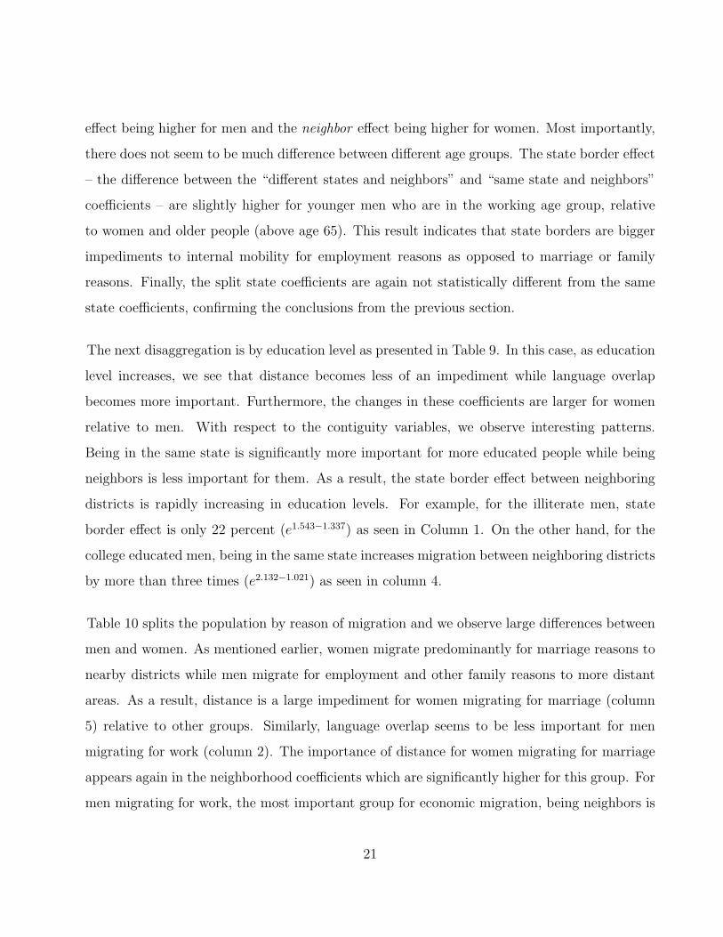
effect being higher for men and the neighbor effect being higher for women. Most importantly,

there does not seem to be much difference between different age groups. The state border effect

– the difference between the “different states and neighbors” and “same state and neighbors”

coefficients – are slightly higher for younger men who are in the working age group, relative

to women and older people (above age 65). This result indicates that state borders are bigger

impediments to internal mobility for employment reasons as opposed to marriage or family

reasons. Finally, the split state coefficients are again not statistically different from the same

state coefficients, confirming the conclusions from the previous section.

The next disaggregation is by education level as presented in Table 9. In this case, as education

level increases, we see that distance becomes less of an impediment while language overlap

becomes more important. Furthermore, the changes in these coefficients are larger for women

relative to men. With respect to the contiguity variables, we observe interesting patterns.

Being in the same state is significantly more important for more educated people while being

neighbors is less important for them. As a result, the state border effect between neighboring

districts is rapidly increasing in education levels. For example, for the illiterate men, state

border effect is only 22 percent (e1.543−1.337) as seen in Column 1. On the other hand, for the

college educated men, being in the same state increases migration between neighboring districts

by more than three times (e2.132−1.021) as seen in column 4.

Table 10 splits the population by reason of migration and we observe large differences between

men and women. As mentioned earlier, women migrate predominantly for marriage reasons to

nearby districts while men migrate for employment and other family reasons to more distant

areas. As a result, distance is a large impediment for women migrating for marriage (column

5) relative to other groups. Similarly, language overlap seems to be less important for men

migrating for work (column 2). The importance of distance for women migrating for marriage

appears again in the neighborhood coefficients which are significantly higher for this group. For

men migrating for work, the most important group for economic migration, being neighbors is

21

significantly less important but the impeding role of the state border is still present and strong.

The final variable of interest is duration of migration which we split into four categories – less

than 1 year, between 1-5 years, between 6-10 years and more than 10 years. This variable

might not capture return migration, especially among the cohorts that migrated in earlier

periods, Nevertheless, the results in Table 11 indicate that there are very little differences in

the coefficients across migration cohorts, with the exception of the most recent group who

arrived within the last year. The neighborhood, same state and state border effects are smaller

for the most recent migrants and even smaller for men.

Another important distinction highlighted in the internal migration literature, especially for

India, is rural-urban migration which is a critical component of economic development and

growth. Many studies explore why rural-to-urban migration is so low India, especially in the

presence of large wage gaps. Our data do not have the urban or rural distinction for the

migrants. So we turn to the population tables published in the Digital Library on the Census

of India website, and construct a variable which represents the share of urban population in a

given district. The values of the variable range between zero and 100. Then we interact this

variable with our contiguity variables, separately for origin and destination districts. For this

estimation, we ignore the issue of split states and include them as different states. Table 12

presents the results for several different groups from the previous tables, chosen for important

differences in their mobility patterns. These groups are: (i) young men and women (age 25-34)

in columns 1 and 2, (ii) illiterate and college educated men in columns 3 and 4, and (iii) women

who migrate for marriage in column 5 and men who migrate for work or business in column 6.

The results in Table 12 highlight several important patterns. The coefficients in the top rows

can be interpreted as the effects from rural to rural districts. The middle section presents

the coefficients when the destination district becomes progressively more urban. The bottom

section shows impact of increasing urbanization in origin districts. It is easier to present these

22

results graphically and we do so in Figure 8. The x-axis is the share of the urban population in

the origin (destination) district on the left (right) and the y-axis is the combined value of the

coefficient. Figure 8(a) is for illiterate male migrants and Figure 8(b) is for college educated

males. (Similar graphs can be constructed for other groups in Table 12.) The red lines on the

top are for value of the combined coefficient for “same state and neighbors” districts while the

blue lines at the bottom are for “different states and neighbors”. For the illiterate migrants in

Figure 8(a), as urbanization level of the origin district increases, the role of the state border, as

depicted by the gap between the lines, declines. For destination districts, urbanization has no

effect on the state border effect. We see a completely different effect for the college educated in

Figure 8(b). As urbanization increases in both origin and destination districts, the state border

effect expands.

Our final set of results utilizes the time dimension in the data. We construct a hypothetical

panel using the duration of migration variable where the dependent variable is now migration

from origin district i to destination district j in year t. We classify the migrants who arrived in

the last year as t = 2001. Migrants who arrived between 1-5 years ago are labelled as t = 1996

and those who arrived between 6-10 years have t = 1991. As mentioned earlier, the return

migration issue might complicate the analysis but we ignore it for the time being. The panel

construction allows us to use destination-year and origin-year fixed effects. We also interact

the year dummies with all of the other bilateral variables. Results in Table 13 show that there

is actually little variation in the values of coefficients over time. For example, year-specific

distance and language variables are not statistically different from each other. Similarly, none

of the contiguity variables are different, indicating their roles in determining migration patterns

are quite stable over time.

23

5 Discussion: some explanations for the invisible wall in

borders

The previous section examines migration costs along three dimensions: 1) the role of geographic

distance and linguistic overlap between the destination and the origin districts of migrants; 2)

the role of neighborhood or contiguity between the destination and the origin districts of mi-

grants; and 3) the role of state boundaries. The role of neighborhood and the role of state

boundaries were delineated by comparing migration between neighboring districts in the same

state and migration between neighboring districts in different states. In this section, we high-

light a number policies, implemented at the state level which act as inhibitors, either explicitly

or implicitly, of mobility across state boundaries. Three key inhibitors of inter-state migration

will be discussed: inadequate portability of social welfare benefits and a significant home bias

in access to education and public employment.

5.1 Inadequate Portability of Social Welfare Benefits

Social welfare entitlements in India, like any country, require proper identification of the recip-

ients. When the recently launched “Unique Identity Documentation” project reaches comple-

tion, India will possess a unified system of national identity documentation. Until then, the

de facto identity document for most Indians households is the “ration card” issued by state

governments. The basic purpose of this card is to enable access to the “Public Distribution

System” (PDS), a program of subsidized food for poor households. But because there is no

national identity documentation system and the PDS covers the majority of the population,

the ration card also serves as the proof of identity needed for access to a wide range of public

services such as hospital care and education. It is also requested as a proof of identity and

address for a variety of other purposes such as initiating telephone service or opening a bank

account (Zelazny, 2012; Abbas and Varma, 2014).

24

Ration cards are not portable across states; that is, they are accepted only by the issuing

state. The main reason has to do with the design of the PDS system for which these cards

were designed. Even though most of the PDS subsidy cost is borne by the central government,

the program is administered by state governments on the basis of their own poverty lines and

lists of poor households. Further, many states add subsidies of their own to the central subsidy

amount. For one, some states have a more inclusive subsidy entitlement policy than the central

government. In Tamil Nadu, for example, every person is entitled to receive subsidized food.

In Andhra Pradesh and Chhattisgarh, more than 70 percent of the population is entitled to

subsidized ration. Secondly, some states provide a bigger price subsidy than that dictated by

the central government. The differences in cost are borne by the state government. As a result,

state governments generally do not extend PDS benefits to migrants who hold ration cards

from other states (Srivastava, 2012).

In order to get access to subsidized food and other public services in their destination state,

inter-state migrants need to surrender the ration card issued by their origin state, and obtain a

new ration card from their destination state. However this process is fraught with difficulties,

particularly for poor and less educated people who are not well-informed about the bureau-

cratic processes and lack social or political connections in the destination state. Procedures for

issuing documentation for the PDS are complicated and vary by state. They are also prone

to corruption and administrative errors. For example, issuing officials in the destination state

may refuse to accept prior identity documentation provided by poor migrants because they are

looking for bribes (Planning Commission, 2008; Abbas and Verma, 2014).

Individuals moving across state boundaries risk losing access to the PDS, and a host of public

services for a substantial period until their destination state issues them a new ration card.

The loss of access to subsidized PDS food could be a significant issue for most households.

According to household survey data, 27 percent of all rural households and 15 percent of all

urban households were fully dependent on PDS grain, and most households in the country were

25

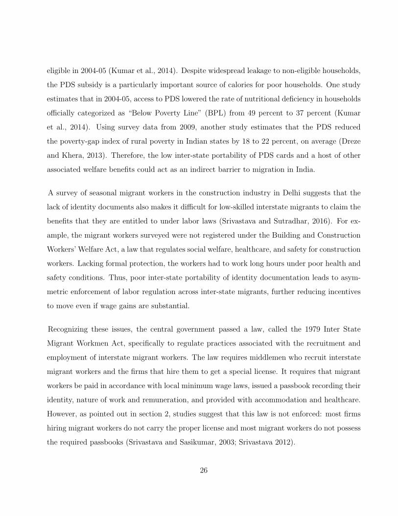
eligible in 2004-05 (Kumar et al., 2014). Despite widespread leakage to non-eligible households,

the PDS subsidy is a particularly important source of calories for poor households. One study

estimates that in 2004-05, access to PDS lowered the rate of nutritional deficiency in households

officially categorized as “Below Poverty Line” (BPL) from 49 percent to 37 percent (Kumar

et al., 2014). Using survey data from 2009, another study estimates that the PDS reduced

the poverty-gap index of rural poverty in Indian states by 18 to 22 percent, on average (Dreze

and Khera, 2013). Therefore, the low inter-state portability of PDS cards and a host of other

associated welfare benefits could act as an indirect barrier to migration in India.

A survey of seasonal migrant workers in the construction industry in Delhi suggests that the

lack of identity documents also makes it difficult for low-skilled interstate migrants to claim the

benefits that they are entitled to under labor laws (Srivastava and Sutradhar, 2016). For ex-

ample, the migrant workers surveyed were not registered under the Building and Construction

Workers’ Welfare Act, a law that regulates social welfare, healthcare, and safety for construction

workers. Lacking formal protection, the workers had to work long hours under poor health and

safety conditions. Thus, poor inter-state portability of identity documentation leads to asym-

metric enforcement of labor regulation across inter-state migrants, further reducing incentives

to move even if wage gains are substantial.

Recognizing these issues, the central government passed a law, called the 1979 Inter State

Migrant Workmen Act, specifically to regulate practices associated with the recruitment and

employment of interstate migrant workers. The law requires middlemen who recruit interstate

migrant workers and the firms that hire them to get a special license. It requires that migrant

workers be paid in accordance with local minimum wage laws, issued a passbook recording their

identity, nature of work and remuneration, and provided with accommodation and healthcare.

However, as pointed out in section 2, studies suggest that this law is not enforced: most firms

hiring migrant workers do not carry the proper license and most migrant workers do not possess

the required passbooks (Srivastava and Sasikumar, 2003; Srivastava 2012).

26

We expect the lack of portability of PDS benefits and cards to contribute to the inertia of the

unskilled who are likely to be most dependent on it. In Figure 9(a), we plot the partial regression

of the share of in-state unskilled emigration on participation in the PDS. The dependent variable

(on the y-axis) is the number of unskilled emigrants who moved to destinations within the

state of their origin, divided by the total number of unskilled migrants from the said state.

This measure comes from the bilateral migration data in the 2001 Census, aggregated to the

state level. The explanatory variable (on the x-axis) is the share of the unskilled population

participating in the Public Distribution System (PDS).13 The regression controls for the log

average household income per capita and the share of agricultural households at the state

level, both of which are also calculated from the NSS data. We find a positive and significant

relationship between the two variables, i.e. the larger the share of unskilled population who

rely on PDS, the higher the tendency for potential emigrants to choose home-state destinations

over out-of-state destinations. This finding is consistent with, and preliminary evidence for, the

argument that inadequate portability of social welfare programs such as PDS tends to deter

households who rely on these benefits from moving across state borders.

5.2 State government employment policies

The state domicile requirements for employment in government entities could act as a disin-

centive to move across states. Under India’s policy of affirmative action, a sizable proportion

of jobs in central and state government entities are reserved for individuals belonging to disad-

vantaged minority groups, principally the Scheduled Castes (SCs) and Scheduled Tribes (STs).

According to the Constitution of India, the percentage of employment quota for SCs and STs in

state government jobs must be equal to their respective shares of a state’s total population. In

1999, on average 25 percent of employment in state-level government jobs was reserved for SCs

13We calculate this measure from the consumption module of the 55th round of National Sample Survey(1999-2000). The unskilled population refers to all members from households with a male household head whohas completed primary education or below. Any household that reported a positive amount of PDS purchaseis considered participating in the PDS, and consequently, so are all individuals from such households.

27

and STs (Howard and Prakash, 2012). In order to be eligible for the SC/ST employment quota

in a particular state, an individual has to belong to an SC/ST community and be domiciled

in that state. Thus, individuals belonging to an SC/ST group would lose access to reserved

government jobs in their home state if they were to migrate to another state.

This disincentive for inter-state migration is likely to matter the most for highly educated

individuals belonging to SC/ST communities but is reportedly also relevant for non-SC/ST

individuals. While the public sector accounts for only about 5 percent of total employment

in India, it is a major employer for educated individuals. On average, 51 percent of wage-

earning individuals with secondary education and above in 2000 were employed in government

jobs (Schundeln and Playforth, 2014). Moreover, the majority of government jobs are with

state government entities. In 2001, 76 percent of government jobs in the median state were

with the state government. Taken together, these numbers suggests that, on average, state

government jobs account for more than 25 percent of employment among individuals with

secondary education and above. Thus, educated individuals, especially but not only SC and

ST individuals, would care about remaining eligible to the employment opportunities in their

home state government.

While all states reserve some government jobs for resident SC/STs and are reported to de

facto prefer residents of that state, some states even have explicit “jobs for natives” policies

that cut across communities. For example, the state of Karnataka announced a policy in 2016

under which both private or public sector firms would have to reserve 70 percent of their jobs

for state residents to be eligible for any state government industrial policy benefits. Orissa,

Maharashtra and Himachal Pradesh have similar quotas for state residents in factory jobs

(Economic Times, 2016). To our knowledge, there is no systematic quantitative evidence on

the extent, enforcement and impact of such policies. Potentially, such policies can create yet

another disincentive to migrate across state boundaries.

28

In Figure 9(b), we plot the partial regression of in-state skilled emigration on public sector

employment at the state level. The dependent variable (on the y-axis) is number of high-skilled

(i.e. those who completed at least secondary education) emigrants who moved to destinations

within the state of their origin, divided by the total number of high-skilled migrants from that

state. The explanatory variable on the x-axis is the share of high-skilled workers who are em-

ployed by the public sector. This variable comes from the employment module of the National

Sample Survey (1999-2000). Log average household income per capita is also calculated from

the NSS data, and controlled for in the regression. The positive relationship shown in the

graph suggests that the higher the share of government job opportunities for the high-skilled,

the stronger the incentive for potential migrants to stay in their home states. The argument

that state domicile requirements for public sector employment inhibit high-skilled workers from

moving across state borders is novel and requires more careful analysis.

5.3 State government policies for access to higher education

Many universities and technical institutes in India are public and under the control of the gov-

ernment of the state in which they are located. For example, in 2003-04, state-level engineering

and “polytechnic” colleges in the state of Tamil Nadu (TN) had a total entering class size of

about 120,000 students (Government of Tamil Nadu, 2004). State residents get preferential

access to state-level colleges and institutes of higher education through “state quota seats”.

The size of the state quota varies by state and by whether the university in question is public

or private, but in general, it is a substantial proportion of the total class size. For example,

in 2004, 50 percent of the seats in all state-level engineering colleges and medical colleges in

Tamil Nadu were under the state quota (Government of Tamil Nadu, 2005). In the state of

Maharashtra, the current state quota in state-level medical colleges varies from 70 percent to

as high as 100 percent (Government of Maharashtra, 2015). In the state of Madhya Pradesh,

38 percent of seats in private medical and dental institutes are in the state quota (Government

29

of Madhya Pradesh, 2014).

“Domicile certificates” are proofs of residence in a state that are issued by state governments

and are necessary to be eligible for the state quota in educational institutes. The certificate is

issued upon proof of continuous residence in the state. The duration of continuous residence

that qualifies an individual for this certificate varies from 3 to 10 years, depending on the state.

For example, the state of Rajasthan issues domicile certificates to individuals who have resided

continuously in the state for at least 10 years, while the state of Uttar Pradesh (UP) requires

continuous residence for at least 3 years (Government of India, 2016).

Domicile requirements for state quota eligibility provide clear and strong disincentives for inter-

state migration. For example, a 16 year old who was born and attended high school in TN

would lose eligibility for state quota seats in state-level universities in Tamil Nadu if his family

were to move to another state, say Uttar Pradesh. Moreover, because of the three-year wait

period for domicile certification in Uttar Pradesh, he would not be eligible for quota seats in

state-level universities there for at least three years. This non-eligibility for state quota seats

in either state would significantly restrict a migrant’s options for higher education compared

to non-migrants and, as a result, reduce incentives to move.

In Figure 9(c), we examine the effect of state government policies determining access to higher

education on emigration for the purpose of education. The dependent variable (on the y-axes)

is the share of the migrants who chose home-state destinations among all migrants who moved

for education related reasons. This variable is constructed from the bilateral data from the 2001

Census as discussed earlier. The explanatory variable on the x-axis comes from the employment

module of the National Sample Survey (1999-2000). It measures the share of college attending

students among all 18-22 year old state-natives in each state. Log average household income per

capita is also calculated from the NSS data, and controlled for in the regression. The positive

slope in the graph is consistent with the argument that state government policies granting

30

preferential access to higher education to in-state students tend to induce potential migrants

moving for education to choose home-state institutions.

6 Conclusion

That international borders limit migration is obvious. More surprising is the role of provincial or

state borders in inhibiting mobility within a country. We are able to demonstrate the existence

of these invisible walls by putting together, with the help of the Indian census authorities,

detailed district-to-district migration data from the 2001 Census. Even after controlling for key

bilateral barriers to mobility, such as physical distance and linguistic differences, and for origin

and destination specific factors through district fixed effects, we find that average migration

between neighboring districts in the same state is at least 50 percent larger than neighboring

districts on different sides of a state border. This gap varies by education level, age and the

reason for migration, but is always large and significant. The evidence from the recent creation

of three new states in 2000 provides additional evidence that these state borders are not natural

barriers.

Since there are no barriers at state borders or explicit legal restrictions on people’s mobility

between states, and we control for distance and difference in language, we investigate other

reasons for the presence of these invisible walls. We argue that interstate mobility is inhibited

by the existence of state level entitlement schemes. The non-portability across state borders

of social welfare benefits, such as access to subsidized food or issuance of PDS ration cards,

weakens the incentive to move for the poor and the unskilled. People are deterred from seeking

education in other states because many universities and technical institutes are under state

control and state residents get preferential access. Finally, the skilled are reluctant to move to

other states to seek employment because state governments are still major employers and grant

de facto preferences to their own residents. We provide preliminary evidence that that the

relative share of migrants moving out-of-state is linked to the importance of these entitlement

31

schemes in each state.

This research can be taken forward in at least three ways. First, the data can be updated

when the Census Bureau releases the data for 2011 and enriched in several ways. The data

tables that were made available to us are two dimensional, for example, we can observe either

the skill composition or the motive for migration in bilateral flows between districts but not

both dimensions simultaneously. Multidimensional data would facilitate richer analysis of the

determinants and consequences of internal migration in India. Second, our analysis of the rea-

sons why state borders restrict mobility is both selective and preliminary at this stage. A fuller

analysis would examine the role of other factors, e.g. such as the National Rural Employment

Guarantee scheme, and for finer evidence of their relative impact. Finally, we motivate this

study by noting that labor mobility enables the reallocation of labor to more productive oppor-

tunities across sectors and regions and hence promotes growth. Future analysis should assess

how far India’s “fragmented entitlements” – i.e. state-level administration of welfare benefits,

as well as education and employment preferences – dampen growth by preventing the efficient

allocation of labor. It may also be possible to assess the impact of the implementation of a

unique national identification system which will lower but not eliminate the costs of moving.

32

Figure

1:Map

ofIndia

in2001

andstatesplits

in2000

(a)2001

India

(b)Splitstates

Source:

Prepared

bytheau

thorsbased

onmigration

data

from

2001censusprovided

byRegistrarGeneraland

Census

Com

mission

er,Governmentof

India.Basemap

isprovided

bytheWorldBank.

Notes:

Threenew

states

werecreatedin

Novem

ber

2000

:Chhattisgarh

(1Novem

ber)wascreatedoutofeasternMadhya

Pradesh;Uttaran

chal

(9Novem

ber),

whichwas

renam

edUttarakhandin

2007,wascreatedoutofthemountainousdistricts

ofnorthwestUttar

Pradesh;an

dJharkhan

d(15Novem

ber)wascreatedoutofthesoutherndistricts

ofBihar.

33

Figure

2:Shareof

inter-districtin-m

igrants

amon

gpop

ulation

atdestinationdistricts

(%)

(a)Male

(b)Fem

ale

Source:

Prepared

bytheau

thorsbased

onmigration

data

from

2001censusprovided

byRegistrarGeneraland

Census

Com

mission

er,Governmentof

India.Basemap

isprovided

bytheWorldBank.

Notes:

This

figu

replots

theeach

district’sshareof

inter-districtin-m

igrants

outoftotalobserved

populationin

2001.Inter-

districtmigrants

referto

thosewhomigrate

across

districts,thusincludeinter-state

andintra-state-inter-districtmigrants.

Theunitof

observationisdistrict,an

dstatebordersareou

tlined

inthicklines.Thereare

593districts

across

35states/union

territoriesin

the2001

Census.

How

ever,9districts

inDelhiare

merged

such

thatDelhiis

asingle

district,leadingto

atotal

of585districts

onthis

map

.

34

Figure

3:Shareof

inter-districtou

t-migrants

amon

gpop

ulation

atorigin

districts

(%)

(a)Male

(b)Fem

ale

Source:

Prepared

bytheau

thorsbased

onmigration

data

from

2001censusprovided

byRegistrarGeneraland

Census

Com

mission

er,Governmentof

India.Basemap

isprovided

bytheWorldBank.

Notes:

Thisfigu

replots

theeach

district’sshareof

inter-districtout-migrants

outoftotalobserved

populationin

2001.Inter-

districtmigrants

referto

thosewhomigrate

across

districts,thusincludeinter-state

andintra-state-inter-districtmigrants.

Theunitof

observationisdistrict,an

dstatebordersareoutlined

inthicklines.Thereare

593districts

across

35states/union

territoriesin

the2001

Census.

How

ever,9districts

inDelhiare

merged

such

thatDelhiis

asingle

district,leadingto

atotal

of58

5districts

onthis

map

.

35

Figure

4:Shareof

inter-statein-m

igrants

amon

gtotalinter-districtin-m

igrants

atdestinationdistricts

(%)

(a)Male

(b)Fem

ale

Source:

Prepared

bytheau

thorsbased

onmigration

data

from

2001censusprovided

byRegistrarGeneraland

Census

Com

mission

er,Governmentof

India.Basemap

isprovided

bytheWorldBank.

Notes:

This

figu

replots

theeach

district’sshareof

inter-state

in-m

igrants

amongobserved

inter-districtin-m

igrants

in2001.Inter-districtmigrants

referto

thosewhomigrate

across

districts,thusincludeinter-state

andintra-state-inter-district

migrants.Theunit

ofob

servationis

district,

andstatebordersare

outlined

inthicklines.Thereare

593districts

across

35states/u

nionterritoriesin

the2001

Census.

How

ever,9districts

inDelhiare

merged

such

thatDelhiis

asingle

district,

lead

ingto

atotalof

585districts

onthis

map

.

36

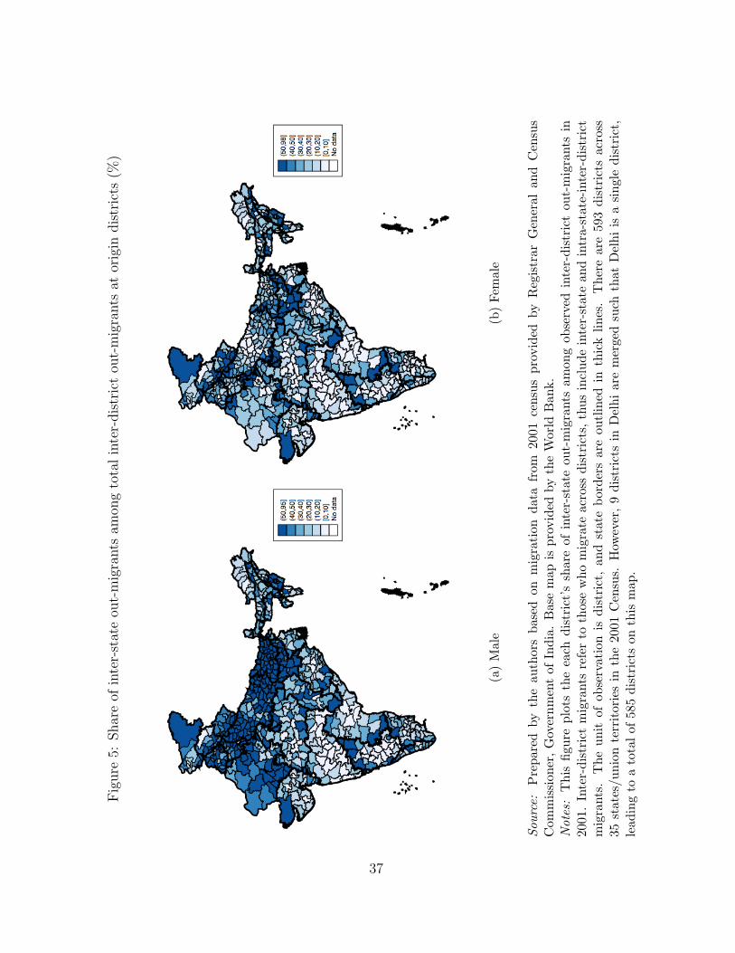
Figure

5:Shareof

inter-stateou

t-migrants

amon

gtotalinter-districtou

t-migrants

atorigin

districts

(%)

(a)Male

(b)Fem

ale

Source:

Prepared

bytheau

thorsbased

onmigration

data

from

2001censusprovided

byRegistrarGeneraland

Census

Com

mission

er,Governmentof

India.Basemap

isprovided

bytheWorldBank.

Notes:

This

figu

replots

theeach

district’sshareof

inter-state

out-migrants

amongobserved

inter-districtout-migrants

in2001

.Inter-districtmigrants

referto

thosewhomigrate

across

districts,thusincludeinter-state

andintra-state-inter-district

migrants.Theunit

ofob

servationis

district,

andstatebordersare

outlined

inthicklines.Thereare

593districts

across

35states/u

nionterritoriesin

the2001

Census.

How

ever,9districts

inDelhiare

merged

such

thatDelhiis

asingle

district,

lead

ingto

atotalof

585districts

onthis

map

.

37

Figure 6: Maharashtra Nagpur as destination

(a)

Andamans

Nicobars

Adilabad

Nizamabad Karimnagar

Medak

HyderabadRangareddi

Mahbubnagar

Nalgonda

Warangal

Khammam

SrikakulamVizianagaram

Visakhapatna

East Godavar

West Godavar

Krishna

Guntur

Prakasam

NelloreCuddapah

Kurnool

Anantapur

Chittoor

Tawang

West KamengEast Kameng

Papum Pare

Lower Subans

Upper SubansWest Siang

East Siang

Upper SiangDibang Valle

Lohit

Changlang

Tirap

Kokrajhar

Dhubri Goalpara

BongaigaonBarpeta

Kamrup

NalbariDarrang

MarigaonNagaon

Sonitpur

Lakhimpur

Dhemaji Tinsukia

Dibrugarh

Sibsagar

Jorhat

Golaghat

Karbi Anglon

North Cachar

Cachar

KarimganjHailakandi

Pashchim Cha

Purba ChampaSheoharSitamarhi

MadhubaniSupaul Araria

Kishanganj

Purnia

Katihar

MadhepuraSaharsa

DarbhangaMuzaffarpur

Gopalganj

Siwan

SaranVaishali Samastipur

BegusaraiKhagaria

Bhagalpur

Banka

MungerLakhisaraiSheikhpuraNalanda

PatnaBhojpurBuxar

Kaimur (BhabRohtas

Jehanabad

AurangabadGaya

Nawada Jamui

Chandigarh

KoriyaSurguja

Jashpur

Raigarh

Korba

Janjgir − Ch

Bilaspur

Kawardha

RajnandgaonDurg

RaipurMahasamund

Dhamtari

Kanker

Bastar

Dantewada

Dadra & Naga

Diu

Daman

North West

North Goa

South Goa

Kachchh

Banas Kantha

Patan

MahesanaSabar Kantha

Gandhinagar

AhmadabadSurendranaga

RajkotJamnagar

Porbandar

Junagadh

Amreli

Bhavnagar

Anand

KhedaPanch MahalsDohad

Vadodara

NarmadaBharuch

Surat

The DangsNavsari

Valsad

Panchkula

AmbalaYamunanagar

Kurukshetra

KaithalKarnal

Panipat

Sonipat

JindFatehabadSirsa

Hisar

Bhiwani

Rohtak

Jhajjar

MahendragarhRewari GurgaonFaridabad

Chamba

Kangra

Lahul & Spit

Kullu

MandiHamirpurUna

Bilaspur

Solan

Sirmaur

Shimla

Kinnaur

Kupwara

BaramulaSrinagar

BadgamPulwamaAnantnag

Leh (Ladakh)

Kargil

Doda

Udhampur

Punch

Rajauri

JammuKathua

Data Not Ava

GarhwaPalamu

Chatra

Hazaribagh

KodarmaGiridih Deoghar

GoddaSahibganj

Pakaur

Dumka

DhanbadBokaro

Ranchi

Lohardaga

Gumla

Pashchimi Si Purbi Singhb

BelgaumBagalkot

Bijapur

Gulbarga

Bidar

Raichur

KoppalGadagDharwad

Uttara Kanna Haveri

Bellary

Chitradurga

Davanagere

Shimoga

Udupi Chikmagalur TumkurKolar

BangaloreBangalore Ru

Mandya

HassanDakshina Kan

KodaguMysore

Chamarajanag

Kasaragod

Kannur

Wayanad

Kozhikode

Malappuram

Palakkad

Thrissur

Ernakulam

Idukki

Kottayam

AlappuzhaPathanamthit

Kollam

Thiruvananth

Lakshadweep

Sheopur

Morena Bhind

GwaliorDatia

Shivpuri

Guna

Tikamgarh

Chhatarpur

Panna

Sagar Damoh

Satna

Rewa

UmariaShahdol

Sidhi

Neemuch

Mandsaur

RatlamUjjain

Shajapur

DewasJhabua

Dhar

Indore

West NimarBarwani East Nimar

Rajgarh Vidisha

Bhopal

Sehore

Raisen

Betul

Harda

Hoshangabad

Katni

Jabalpur

Narsimhapur Dindori

Mandla

Chhindwara

Seoni

Balaghat

Nandurbar

Dhule

Jalgaon

Buldana

Akola

Washim

Amravati

Wardha

Nagpur BhandaraGondiya

Gadchiroli

ChandrapurYavatmal

Nanded

Hingoli

Parbhani

Jalna

Aurangabad

Nashik

Thane

Mumbai (Subu

Mumbai

Raigarh Pune

Ahmadnagar

Bid

Latur

Osmanabad

SolapurSatara

Ratnagiri

Sindhudurg

Kolhapur

Sangli

Senapati (Ex

Tamenglong

Churachandpu

BishnupurThoubalImphal West

Imphal East

Ukhrul

Chandel

West Garo HiEast Garo Hi

South Garo H

West Khasi H

Ri Bhoi

East Khasi HJaintia Hill

Mamit

Kolasib

Aizawl

Champhai

Serchhip

Lunglei

LawngtlaiSaiha

Mon

Tuensang

Mokokchung

ZunhebotoWokha

DimapurKohima Phek

Bargarh

Jharsuguda

SambalpurDebagarh

Sundargarh

Kendujhar

Mayurbhanj

Baleshwar

Bhadrak

Kendrapara

Jagatsinghap

Cuttack

JajapurDhenkanalAnugul

NayagarhKhordha

Puri

Ganjam

Gajapati

Kandhamal

Baudh

Sonapur

BalangirNuapada

Kalahandi

Rayagada

Nabarangapur

Koraput

Malkangiri

Yanam

Pondicherry

Mahe

Karaikal

Gurdaspur

Amritsar

KapurthalaJalandhar

Hoshiarpur

NawanshahrRupnagar

Fatehgarh Sa

LudhianaMoga

Firozpur

Muktsar

Faridkot

Bathinda

Mansa

Sangrur Patiala

GanganagarHanumangarh

BikanerChuru

Jhunjhunun

Alwar

Bharatpur

DhaulpurKarauli

Sawai Madhop

DausaJaipur

Sikar

Nagaur

Jodhpur

Jaisalmer

Barmer

Jalor

Sirohi

Pali

AjmerTonk

BundiBhilwara

Rajsamand

Udaipur

Dungarpur

Banswara

Chittaurgarh

KotaBaran

Jhalawar

North

WestSouth East

Thiruvallur

Chennai

KancheepuramVellore

DharmapuriTiruvannamal

Viluppuram

Salem

NamakkalErodeThe Nilgiris

Coimbatore

Dindigul

KarurTiruchirappa

PerambalurAriyalur

Cuddalore

Nagapattinam

ThiruvarurThanjavur

Pudukkottai

SivagangaMaduraiTheni

VirudhunagarRamanathapur

ThoothukkudiTirunelveli

Kanniyakumar

West Tripura

South Tripur

Dhalai

North Tripur

Saharanpur

Muzaffarnaga Bijnor

MoradabadRampurJyotiba Phul

MeerutBaghpat

Ghaziabad

Gautam BuddhBulandshahr

Aligarh

HathrasMathura

AgraFirozabad

Etah

Mainpuri

Budaun

BareillyPilibhit

ShahjahanpurKheri

Sitapur

Hardoi

Unnao

Lucknow

Rae Bareli

Farrukhabad

Kannauj

EtawahAuraiya

Kanpur DehatKanpur Nagar

Jalaun

Jhansi

Lalitpur

Hamirpur

MahobaBanda

Chitrakoot

Fatehpur Pratapgarh

Kaushambi

Allahabad

Barabanki

Faizabad

Ambedkar NagSultanpur

BahraichShrawasti

Balrampur

Gonda

Siddharthnag

BastiSant Kabir N

Mahrajganj

Gorakhpur

Kushinagar

Deoria

Azamgarh MauBallia

JaunpurGhazipur

Chandauli

VaranasiSant Ravidas

Mirzapur

Sonbhadra

Uttarkashi

ChamoliRudraprayagTehri GarhwaDehradun

Garhwal

PithoragarhBageshwar

Almora

ChampawatNainital

Udham Singh

Hardwar

Darjiling

Jalpaiguri

Koch Bihar

Uttar Dinajp

Dakshin Dina

Maldah

Murshidabad

Birbhum

Barddhaman Nadia

North Twenty

Hugli

BankuraPuruliya

Medinipur

HaoraKolkata

South Twent

(10,12](8,10](6,8](4,6](2,4](1,2](.5,1](.1,.5][0,.1]Origin

(b)

Source: Prepared by the authors based on migration data from 2001 census provided by RegistrarGeneral and Census Commissioner, Government of India. Base map is provided by the World Bank.Notes: State borders are outlined in thick lines. In this figure, we focus on Nagpur (in the state ofMaharashtra) as a destination district and we plot the origin districts of migrants coming to Nagpur.Nagpur is highlighted in red in the middle of the maps, and all other origin districts are in ascendingshades of blue depending on the share of migrants they send. Part (b) of this figure zooms in onNagpur and its surrounding districts.

38

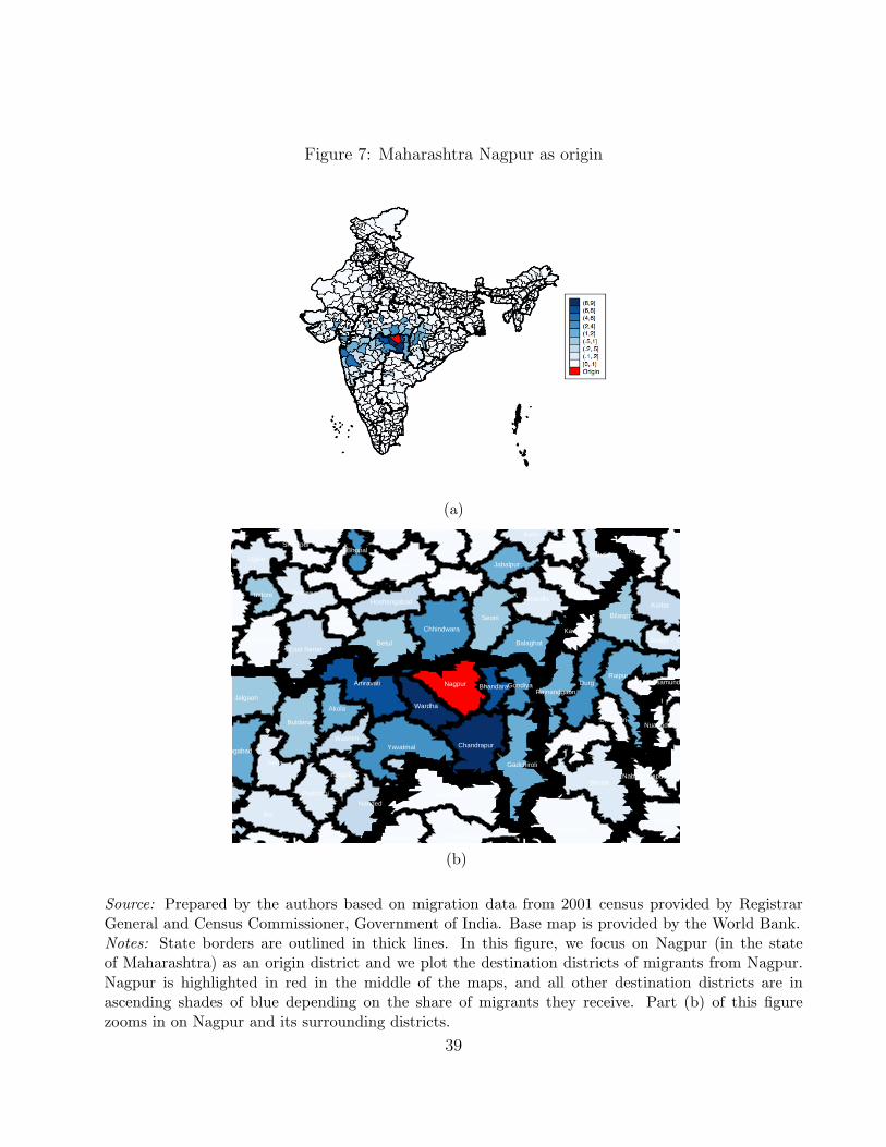
Figure 7: Maharashtra Nagpur as origin

(a)

Andamans

Nicobars

Adilabad

Nizamabad Karimnagar

Medak

HyderabadRangareddi

Mahbubnagar

Nalgonda

Warangal

Khammam

SrikakulamVizianagaram

Visakhapatna

East Godavar

West Godavar

Krishna

Guntur

Prakasam

NelloreCuddapah

Kurnool

Anantapur

Chittoor

Tawang

West KamengEast Kameng

Papum Pare

Lower Subans

Upper SubansWest Siang

East Siang

Upper SiangDibang Valle

Lohit

Changlang

Tirap

Kokrajhar

Dhubri Goalpara

BongaigaonBarpeta

Kamrup

NalbariDarrang

MarigaonNagaon

Sonitpur

Lakhimpur

Dhemaji Tinsukia

Dibrugarh

Sibsagar

Jorhat

Golaghat

Karbi Anglon

North Cachar

Cachar

KarimganjHailakandi

Pashchim Cha

Purba ChampaSheoharSitamarhi

MadhubaniSupaul Araria

Kishanganj

Purnia

Katihar

MadhepuraSaharsa

DarbhangaMuzaffarpur

Gopalganj

Siwan

SaranVaishali Samastipur

BegusaraiKhagaria

Bhagalpur

Banka

MungerLakhisaraiSheikhpuraNalanda

PatnaBhojpurBuxar

Kaimur (BhabRohtas

Jehanabad

AurangabadGaya

Nawada Jamui

Chandigarh

KoriyaSurguja

Jashpur

Raigarh

Korba

Janjgir − Ch

Bilaspur

Kawardha

RajnandgaonDurg

RaipurMahasamund

Dhamtari

Kanker

Bastar

Dantewada

Dadra & Naga

Diu

Daman

North West

North Goa

South Goa

Kachchh

Banas Kantha

Patan

MahesanaSabar Kantha

Gandhinagar

AhmadabadSurendranaga

RajkotJamnagar

Porbandar

Junagadh

Amreli

Bhavnagar

Anand

KhedaPanch MahalsDohad

Vadodara

NarmadaBharuch

Surat

The DangsNavsari

Valsad

Panchkula

AmbalaYamunanagar

Kurukshetra

KaithalKarnal

Panipat

Sonipat

JindFatehabadSirsa

Hisar

Bhiwani

Rohtak

Jhajjar

MahendragarhRewari GurgaonFaridabad

Chamba

Kangra

Lahul & Spit

Kullu

MandiHamirpurUna

Bilaspur

Solan

Sirmaur

Shimla

Kinnaur

Kupwara

BaramulaSrinagar

BadgamPulwamaAnantnag

Leh (Ladakh)

Kargil

Doda

Udhampur

Punch

Rajauri

JammuKathua

Data Not Ava

GarhwaPalamu

Chatra

Hazaribagh

KodarmaGiridih Deoghar

GoddaSahibganj

Pakaur

Dumka

DhanbadBokaro

Ranchi

Lohardaga

Gumla

Pashchimi Si Purbi Singhb

BelgaumBagalkot

Bijapur

Gulbarga

Bidar

Raichur

KoppalGadagDharwad

Uttara Kanna Haveri

Bellary

Chitradurga

Davanagere

Shimoga

Udupi Chikmagalur TumkurKolar

BangaloreBangalore Ru

Mandya

HassanDakshina Kan

KodaguMysore

Chamarajanag

Kasaragod

Kannur

Wayanad

Kozhikode

Malappuram

Palakkad

Thrissur

Ernakulam

Idukki

Kottayam

AlappuzhaPathanamthit

Kollam

Thiruvananth

Lakshadweep

Sheopur

Morena Bhind

GwaliorDatia

Shivpuri

Guna

Tikamgarh

Chhatarpur

Panna

Sagar Damoh

Satna

Rewa

UmariaShahdol

Sidhi

Neemuch

Mandsaur

Ratlam

Ujjain

Shajapur

DewasJhabua

Dhar

Indore

West NimarBarwani East Nimar

Rajgarh Vidisha

Bhopal

Sehore

Raisen

Betul

Harda

Hoshangabad

Katni

Jabalpur

Narsimhapur Dindori

Mandla

Chhindwara

Seoni

Balaghat

Nandurbar

Dhule

Jalgaon

Buldana

Akola

Washim

Amravati

Wardha

Nagpur BhandaraGondiya

Gadchiroli

ChandrapurYavatmal

Nanded

Hingoli

Parbhani

Jalna

Aurangabad

Nashik

Thane

Mumbai (Subu

Mumbai

Raigarh Pune

Ahmadnagar

Bid

Latur

Osmanabad

SolapurSatara

Ratnagiri

Sindhudurg

Kolhapur

Sangli

Senapati (Ex

Tamenglong

Churachandpu

BishnupurThoubalImphal West

Imphal East

Ukhrul

Chandel

West Garo HiEast Garo Hi

South Garo H

West Khasi H

Ri Bhoi

East Khasi HJaintia Hill

Mamit

Kolasib

Aizawl

Champhai

Serchhip

Lunglei

LawngtlaiSaiha

Mon

Tuensang

Mokokchung

ZunhebotoWokha

DimapurKohima Phek

Bargarh

Jharsuguda

SambalpurDebagarh

Sundargarh

Kendujhar

Mayurbhanj

Baleshwar

Bhadrak

Kendrapara

Jagatsinghap

Cuttack

JajapurDhenkanalAnugul

NayagarhKhordha

Puri

Ganjam

Gajapati

Kandhamal

Baudh

Sonapur

BalangirNuapada

Kalahandi

Rayagada

Nabarangapur

Koraput

Malkangiri

Yanam

Pondicherry

Mahe

Karaikal

Gurdaspur

Amritsar

KapurthalaJalandhar

Hoshiarpur

NawanshahrRupnagar

Fatehgarh Sa

LudhianaMoga

Firozpur

Muktsar

Faridkot

Bathinda

Mansa

Sangrur Patiala

GanganagarHanumangarh

BikanerChuru

Jhunjhunun

Alwar

Bharatpur

DhaulpurKarauli

Sawai Madhop

DausaJaipur

Sikar

Nagaur

Jodhpur

Jaisalmer

Barmer

Jalor

Sirohi

Pali

AjmerTonk

BundiBhilwara

Rajsamand

Udaipur

Dungarpur

Banswara

Chittaurgarh

KotaBaran

Jhalawar

North

WestSouth East

Thiruvallur

Chennai

KancheepuramVellore

DharmapuriTiruvannamal

Viluppuram

Salem

NamakkalErodeThe Nilgiris

Coimbatore

Dindigul

KarurTiruchirappa

PerambalurAriyalur

Cuddalore

Nagapattinam

ThiruvarurThanjavur

Pudukkottai

SivagangaMaduraiTheni

VirudhunagarRamanathapur

ThoothukkudiTirunelveli

Kanniyakumar

West Tripura

South Tripur

Dhalai

North Tripur

Saharanpur

Muzaffarnaga Bijnor

MoradabadRampurJyotiba Phul

MeerutBaghpat

Ghaziabad

Gautam BuddhBulandshahr

Aligarh

HathrasMathura

AgraFirozabad

Etah

Mainpuri

Budaun

BareillyPilibhit

ShahjahanpurKheri

Sitapur

Hardoi

Unnao

Lucknow

Rae Bareli

Farrukhabad

Kannauj

EtawahAuraiya

Kanpur DehatKanpur Nagar

Jalaun

Jhansi

Lalitpur

Hamirpur

MahobaBanda

Chitrakoot

Fatehpur Pratapgarh

Kaushambi

Allahabad

Barabanki

Faizabad

Ambedkar NagSultanpur

BahraichShrawasti

Balrampur

Gonda

Siddharthnag

BastiSant Kabir N

Mahrajganj

Gorakhpur

Kushinagar

Deoria

Azamgarh MauBallia

JaunpurGhazipur

Chandauli

VaranasiSant Ravidas

Mirzapur

Sonbhadra

Uttarkashi

ChamoliRudraprayagTehri GarhwaDehradun

Garhwal

PithoragarhBageshwar

Almora

ChampawatNainital

Udham Singh

Hardwar

Darjiling

Jalpaiguri

Koch Bihar

Uttar Dinajp

Dakshin Dina

Maldah

Murshidabad

Birbhum

Barddhaman Nadia

North Twenty

Hugli

BankuraPuruliya

Medinipur

HaoraKolkata

South Twent

(8,9](6,8](4,6](2,4](1,2](.5,1](.2,.5](.1,.2][0,.1]Origin

(b)

Source: Prepared by the authors based on migration data from 2001 census provided by RegistrarGeneral and Census Commissioner, Government of India. Base map is provided by the World Bank.Notes: State borders are outlined in thick lines. In this figure, we focus on Nagpur (in the stateof Maharashtra) as an origin district and we plot the destination districts of migrants from Nagpur.Nagpur is highlighted in red in the middle of the maps, and all other destination districts are inascending shades of blue depending on the share of migrants they receive. Part (b) of this figurezooms in on Nagpur and its surrounding districts.

39

Figure 8: Estimated border effect

.6.8

11.

2

0 20 40 60 80 100Share of urban population at origin district (%)

Different states, neighbor

Same state, neighbor

.6.8

11.

21.

41.

6

0 20 40 60 80 100Share of urban population at destination district (%)

Different states, neighbor

Same state, neighbor

Estimated border effects: illiterate male inter−district migrants

(a) Illiterate males

.51

1.5

2

0 20 40 60 80 100Share of urban population at origin district (%)

Different states, neighbor

Same state, neighbor

.51

1.5

2

0 20 40 60 80 100Share of urban population at destination district (%)

Different states, neighbor

Same state, neighbor

Estimated border effects: male inter−district migrants with college degree

(b) Males with college degree

Source: Prepared by the authors based on PPML gravity estimation in Table 12.Notes: This figure plots the estimated border-contiguity coefficients from PPML gravity estimation(Table 12) against shares of urban population at origin and destination districts, respectively.

40

Figure 9: Institutional Barriers and Migration Inertia

Daman & Diu

Manipur

Jharkhand

Punjab

Maharashtra

GoaBihar

Rajasthan

Pondicherry

Meghalaya

Haryana

Madhya Pradesh

Andhra PradeshUttar PradeshGujarat

KarnatakaKerala

Mizoram

Himachal PradeshTamil Nadu

West BengalAssamOrissa

Jammu & KashmirTripura

A & N Islands

Chhattisgarh

Uttranchal

Arunachal Pradesh

Sikkim

−60

−40

−20

020

40S

hare

of i

n−st

ate

emig

rant

s am

ong

all u

nski

lled

emig

rant

s (%

)

−20 −10 0 10 20Participation in PDS (%)

Partial Regression Coef. = 0.805, SE = 0.328, t = 2.46

Control variables: Log average household income per capita, Share of agricultural populationSample from NSS: people from households with unskilled male household headsSample from Census: migrants with primary education or below

Participation in Public Distribution System and Unskilled Out−migration (%)

(a) Public Distribution System

Arunachal Pradesh

Tripura

Daman & Diu

JharkhandHaryana

Bihar

Goa

West BengalJammu & KashmirGujarat

Kerala

Uttar Pradesh

Punjab

Maharashtra

Tamil NaduKarnataka

Andhra Pradesh

Himachal Pradesh

Uttranchal

Mizoram

ManipurAssam

Nagaland

Rajasthan

Madhya Pradesh

Pondicherry

OrissaChhattisgarh

A & N Islands

Meghalaya

Sikkim

−40

−20

020

40S

hare

of i

n−st

ate

emig

rant

s am

ong

all h

igh−

skill

ed e

mig

rant

s (%

)

−20 −10 0 10 20 30Share of public employees among high−skilled employees (%)

Partial Regression Coef.= 0.804, SE = 0.408, t = 1.97

Control variable: Log average household income per capitaSample from NSS: wage earning males with secondary education or aboveSample from Census: migrants with secondary education or above

Public Sector Employment and Skilled Out−migration

(b) Public employment of the high-skilled

41

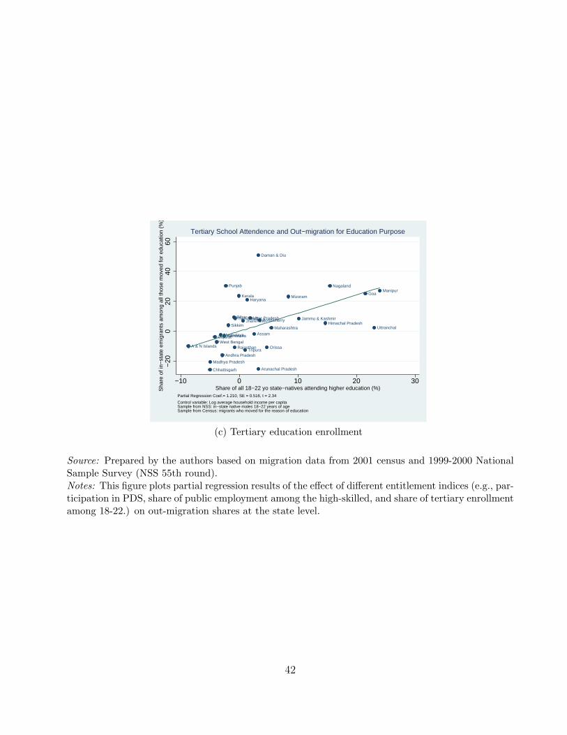
A & N Islands

Chhattisgarh

Madhya Pradesh

GujaratWest Bengal

Meghalaya

Andhra Pradesh

Karnataka

Punjab

Sikkim

Bihar

Rajasthan

Tamil Nadu

Kerala

Jharkhand

Tripura

Haryana

Uttar Pradesh

Assam

Daman & Diu

Arunachal Pradesh

Pondicherry

Orissa

Maharashtra

Mizoram

Jammu & KashmirHimachal Pradesh

Nagaland

Goa

Uttranchal

Manipur

−20

020

4060

Sha

re o

f in−

stat

e em

igra

nts

amon

g al

l tho

se m

oved

for

educ

atio

n (%

)

−10 0 10 20 30Share of all 18−22 yo state−natives attending higher education (%)

Partial Regression Coef.= 1.210, SE = 0.516, t = 2.34

Control variable: Log average household income per capitaSample from NSS: in−state native males 18−22 years of ageSample from Census: migrants who moved for the reason of education

Tertiary School Attendence and Out−migration for Education Purpose

(c) Tertiary education enrollment

Source: Prepared by the authors based on migration data from 2001 census and 1999-2000 NationalSample Survey (NSS 55th round).Notes: This figure plots partial regression results of the effect of different entitlement indices (e.g., par-ticipation in PDS, share of public employment among the high-skilled, and share of tertiary enrollmentamong 18-22.) on out-migration shares at the state level.

42

Table 1: Population distribution by gender and resident type MALE FEMALE

Resident Type

Native (non-migrant)

Intra-district migrant

Intra-state-inter-district

migrant Inter-state

migrant Total Native (non-

migrant) Intra-district

migrant

Intra-state-inter-district

migrant Inter-state

migrant Total Total # (thousand)

445,373 47,338 22,468 16,978 532,157

281,735 146,255 48,639 19,825 496,454

Share (%) in population 83.7 8.9 4.2 3.2 100.0 56.7 29.5 9.8 4.0 100.0 Source: Prepared by the authors based on migration data from 2001 census provided by Registrar General and Census Commissioner, Government of India. Notes: This table describes the population distribution of India by gender and resident type in 2001. First row reports the total count, and the second row reports the share of a group in total population. “Native (non-migrant)” refers to those who didn’t move; “Intra-district migrant” to one who moved within the district; “Intra-state-inter-district migrant” to those who moved to a different district within the state; and “Inter-state migrant” to those who moved to a different state. Our sample excludes those who reported last usual residence as “unknown”.

Table 2: Demographic distribution of population by gender, resident type, and age MALE FEMALE

Resident Type

Native (non-migrant)

Intra-district migrant

Intra-state-inter-district

migrant Inter-state

migrant Total Native (non-

migrant) Intra-district

migrant

Intra-state-inter-district

migrant Inter-state

migrant Total AGE GROUP (%) (%) (%) (%) (thousand) (%) (%) (%) (%) (thousand) 0-13

89.6 6.9 2.3 1.2 177,675

89.6 7.0 2.2 1.2 163,348

14-19

85.7 8.4 3.4 2.5 65,753

76.8 15.9 5.2 2.1 57,051 20-24

82.5 8.5 4.5 4.4 46,321

42.0 39.4 13.4 5.2 43,443

25-34

80.0 9.7 5.4 4.9 78,919

30.9 46.3 16.2 6.6 78,777 35-44

77.7 11.2 6.3 4.9 65,917

29.7 47.3 16.3 6.6 60,395

45-54

77.1 11.5 6.6 4.8 44,719

30.8 47.4 15.6 6.2 39,277 55-64

79.7 10.6 5.7 4.0 27,169

32.2 48.2 14.4 5.3 28,001

65+

82.2 9.9 4.8 3.2 24,182

35.9 45.4 13.7 5.0 24,924 Age not stated 85.1 9.1 3.8 2.0 1,501 68.6 21.9 7.2 2.4 1,238

Source: Prepared by the authors based on migration data from 2001 census provided by Registrar General and Census Commissioner, Government of India. Notes: This table describes the demographic distribution of 2001 India population by gender and resident type. Definitions of 4 types of residents are introduced in Table 1. Each cell reports the shares of different resident types in a certain age group. Total population of each age group is listed in the “Total” columns.

43

Table 3: Demographic distribution of population by gender, resident type, and education levels MALE FEMALE

Resident Type

Native (non-migrant)

Intra-district migrant

Intra-state-inter-district

migrant Inter-state

migrant Total Native (non-

migrant) Intra-district

migrant

Intra-state-inter-district

migrant Inter-state

migrant Total EDUCATION LEVEL (%) (%) (%) (%) (thousand) (%) (%) (%) (%) (thousand) Illiterate

88.5 7.1 2.3 2.1 195,623

54.2 33.6 8.7 3.5 272,299

Primary

85.2 8.9 3.4 2.5 176,035

63.8 24.6 8.5 3.1 135,560 All Secondary

78.4 10.7 6.3 4.7 134,898

54.9 25.3 14.1 5.7 76,428

College Degree +

64.4 13.5 13.7 8.4 25,533

47.2 18.3 21.7 12.8 12,137 Education level unknown 100.0 0.0 0.0 0.0 68 100.0 0.0 0.0 0.0 30 Source: Prepared by the authors based on migration data from 2001 census provided by Registrar General and Census Commissioner, Government of India. Notes: This table describes the distribution of education levels in the male and female populations in India, 2001. It follows the same structure as Table 2. Education level is the highest degree that an individual has completed. “All Secondary” includes Lower Secondary, High Secondary (or Senior Secondary) degrees, and vocational/professional diplomas. “College +” includes undergraduate degrees and above.

Table 4: Distribution of migrants by gender, migrant type, and reason for migration MALE FEMALE

Resident Type

Intra-district migrant

Intra-state-inter-district

migrant Inter-state

migrant Total Intra-district

migrant

Intra-state-inter-district

migrant Inter-state

migrant Total REASON FOR MIGRATION (%) (%) (%) (thousand) (%) (%) (%) (thousand) Work or Business

30.1 34.0 35.9 26,867

43.8 34.6 21.6 3,902

Marriage

70.6 22.0 7.4 2,125

71.2 21.5 7.3 151,656 Move with Family

53.9 29.6 16.5 25,590

48.5 31.5 20.0 29,402

Education

49.7 34.9 15.4 2,266

54.9 32.8 12.4 939 Other Reason 76.3 15.0 8.7 29,935 75.5 17.6 6.9 28,819

Source: Prepared by the authors based on migration data from 2001 census provided by Registrar General and Census Commissioner, Government of India. Notes: This table describes the distribution of migrants based on the “reasons of migration”, which include: work, business, marriage, move with family, education, and other reason (unspecified). Row percentages are reported, as well as total counts of migrants for each reason.

44

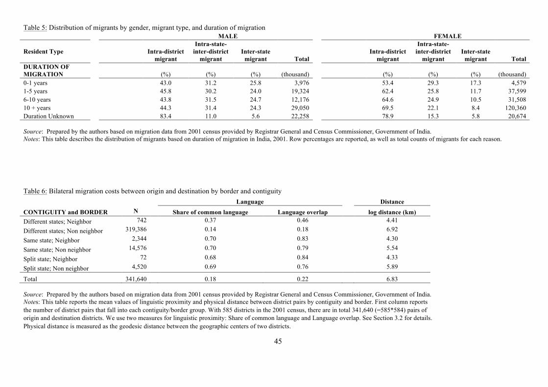
Table 5: Distribution of migrants by gender, migrant type, and duration of migration MALE FEMALE

Resident Type

Intra-district migrant

Intra-state-inter-district

migrant Inter-state

migrant Total Intra-district

migrant

Intra-state-inter-district

migrant Inter-state

migrant Total DURATION OF MIGRATION (%) (%) (%) (thousand) (%) (%) (%) (thousand) 0-1 years

43.0 31.2 25.8 3,976

53.4 29.3 17.3 4,579

1-5 years

45.8 30.2 24.0 19,324

62.4 25.8 11.7 37,599 6-10 years

43.8 31.5 24.7 12,176

64.6 24.9 10.5 31,508

10 + years

44.3 31.4 24.3 29,050

69.5 22.1 8.4 120,360 Duration Unknown 83.4 11.0 5.6 22,258 78.9 15.3 5.8 20,674 Source: Prepared by the authors based on migration data from 2001 census provided by Registrar General and Census Commissioner, Government of India. Notes: This table describes the distribution of migrants based on duration of migration in India, 2001. Row percentages are reported, as well as total counts of migrants for each reason.

Table 6: Bilateral migration costs between origin and destination by border and contiguity

Language

Distance CONTIGUITY and BORDER N Share of common language Language overlap

log distance (km)

Different states; Neighbor 742 0.37 0.46 4.41

Different states; Non neighbor 319,386 0.14 0.18

6.92

Same state; Neighbor 2,344 0.70 0.83 4.30

Same state; Non neighbor 14,576 0.70 0.79

5.54

Split state; Neighbor 72 0.68 0.84 4.33

Split state; Non neighbor 4,520 0.69 0.76 5.89

Total 341,640 0.18 0.22

6.83 Source: Prepared by the authors based on migration data from 2001 census provided by Registrar General and Census Commissioner, Government of India. Notes: This table reports the mean values of linguistic proximity and physical distance between district pairs by contiguity and border. First column reports the number of district pairs that fall into each contiguity/border group. With 585 districts in the 2001 census, there are in total 341,640 (=585*584) pairs of origin and destination districts. We use two measures for linguistic proximity: Share of common language and Language overlap. See Section 3.2 for details. Physical distance is measured as the geodesic distance between the geographic centers of two districts.

45

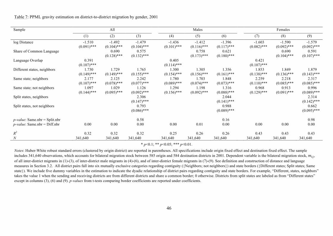
Table 7: PPML gravity estimation on district-to-district migration by gender, 2001

Sample All Males Females (1) (2) (3) (4) (5) (6) (7) (8) (9) log Distance -1.510 -1.492 -1.479 -1.436 -1.412 -1.396 -1.603 -1.590 -1.579 (0.091)*** (0.104)*** (0.104)*** (0.101)*** (0.116)*** (0.117)*** (0.082)*** (0.092)*** (0.092)*** Share of Common Language 0.690 0.575 0.758 0.621 0.690 0.591 (0.128)*** (0.132)*** (0.173)*** (0.180)*** (0.104)*** (0.107)*** Language Overlap 0.391 0.405 0.421 (0.107)*** (0.114)*** (0.107)*** Different states, neighbors 1.730 1.729 1.765 1.300 1.305 1.356 1.853 1.849 1.879 (0.149)*** (0.149)*** (0.155)*** (0.154)*** (0.156)*** (0.161)*** (0.138)*** (0.136)*** (0.143)*** Same state; neighbors 2.177 2.125 2.242 1.780 1.703 1.848 2.259 2.218 2.317 (0.107)*** (0.078)*** (0.077)*** (0.089)*** (0.074)*** (0.073)*** (0.110)*** (0.085)*** (0.085)*** Same state; not neighbors 1.097 1.029 1.126 1.294 1.198 1.316 0.968 0.913 0.996 (0.144)*** (0.095)*** (0.092)*** (0.156)*** (0.092)*** (0.088)*** (0.129)*** (0.091)*** (0.089)*** Split states, neighbors 2.306 2.044 2.314 (0.147)*** (0.141)*** (0.142)*** Split states, not neighbors 0.793 0.988 0.662 (0.086)*** (0.089)*** (0.095)*** p-value: Same.nbr = Split.nbr 0.58 0.16 0.98 p-value: Same.nbr = Diff.nbr 0.00 0.00 0.00 0.00 0.01 0.00 0.00 0.00 0.00 R2 0.32 0.32 0.32 0.25 0.26 0.26 0.43 0.43 0.43 N 341,640 341,640 341,640 341,640 341,640 341,640 341,640 341,640 341,640

* p<0.1; ** p<0.05; *** p<0.01. Notes: Huber-White robust standard errors (clustered by origin district) are reported in parentheses. All specifications include origin fixed effect and destination fixed effect. The sample includes 341,640 observations, which accounts for bilateral migration stock between 585 origin and 584 destination districts in 2001. Dependent variable is the bilateral migration stock, 𝑚!", of all inter-district migrants in (1)-(3), of inter-district male migrants in (4)-(6), and of inter-district female migrants in (7)-(9). See definition and construction of distance and language measures in Section 3.2. All district pairs fall into six mutually exclusive categories regarding contiguity ({Neighbors; not neighbors}) and state borders ({Different states; Split states; Same state}). We include five dummy variables in the estimation to indicate the dyadic relationship of district pairs regarding contiguity and state borders. For example, “Different, states, neighbors” takes the value 1 when the sending and receiving districts are from different districts and share a common border; 0 otherwise. Districts from split states are labeled as from “Different states” except in columns (3), (6) and (9). p-values from t-tests comparing border coefficients are reported under coefficients.

46

Table 8: PPML gravity estimation on district-to-district migration by gender and age, 2001

Males Females Ages 25-34 35-64 65 + 25-34 35-64 65+ log Distance -1.394 -1.467 -1.493 -1.581 -1.630 -1.715 (0.123)*** (0.112)*** (0.128)*** (0.088)*** (0.092)*** (0.091)*** Share of Common Language 0.589 0.533 0.760 0.583 0.558 0.612 (0.200)*** (0.167)*** (0.177)*** (0.103)*** (0.109)*** (0.122)*** Different states, neighbors 1.327 1.222 1.278 1.916 1.852 1.916 (0.171)*** (0.155)*** (0.160)*** (0.144)*** (0.143)*** (0.135)*** Same state; neighbors 1.820 1.715 1.542 2.375 2.272 2.268 (0.085)*** (0.076)*** (0.077)*** (0.086)*** (0.087)*** (0.096)*** Same state; not neighbors 1.374 1.315 1.049 0.985 0.929 0.831 (0.089)*** (0.086)*** (0.100)*** (0.083)*** (0.088)*** (0.091)*** Split states, neighbors 2.210 1.956 1.709 2.395 2.247 2.159 (0.146)*** (0.132)*** (0.176)*** (0.137)*** (0.144)*** (0.162)*** Split states, not neighbors 1.012 1.046 0.777 0.629 0.689 0.482 (0.100)*** (0.086)*** (0.093)*** (0.095)*** (0.100)*** (0.127)*** p-value: Same.nbr = Split.nbr 0.01 0.08 0.33 0.84 0.81 0.39 p-value: Same.nbr = Diff.nbr 0.01 0.00 0.10 0.00 0.00 0.00 R2 0.27 0.30 0.36 0.48 0.49 0.58 N 341,640 341,640 341,640 341,640 341,640 341,640

* p<0.1; ** p<0.05; *** p<0.01. Notes: Huber-White robust standard errors (clustered by origin district) are reported in parentheses. All specifications include origin fixed effect and destination fixed effect. The sample includes 341,640 observations, which accounts for bilateral migration stock between 585 origin and 584 destination districts in 2001. Dependent variable is the bilateral migration stock, 𝑚!", of inter-district male migrants by age group, and of inter-district female migrants by age group. See Table 2 for the age composition of males and females. Definition and construction of distance and language measures are described in Section 3.2. All district pairs fall into six mutually exclusive categories regarding contiguity ({Neighbors; not neighbors}) and state borders ({Different states; Split states; Same state}). We include five dummy variables in the estimation to indicate the dyadic relationship of district pairs regarding contiguity and state borders. For example, “Different, states, neighbors” takes the value 1 when the sending and receiving districts are from different districts and share a common border; 0 otherwise. p-values from t-tests comparing border coefficients are reported under coefficients.

47

Table 9: PPML gravity estimation on district-to-district migration by gender and education attainment, 2001

Males Females Education Attainment Illiterate Primary All

Secondary College + Illiterate Primary All

Secondary College +

log Distance -1.646 -1.499 -1.368 -1.134 -1.705 -1.632 -1.524 -1.184 (0.102)*** (0.139)*** (0.121)*** (0.094)*** (0.077)*** (0.112)*** (0.084)*** (0.083)*** Share of Common Language 0.539 0.613 0.580 0.902 0.388 0.653 0.701 0.981 (0.176)*** (0.199)*** (0.192)*** (0.161)*** (0.110)*** (0.119)*** (0.114)*** (0.160)*** Different states, neighbors 1.337 1.492 1.193 1.021 2.064 1.876 1.360 0.854 (0.142)*** (0.179)*** (0.173)*** (0.141)*** (0.122)*** (0.157)*** (0.138)*** (0.130)*** Same state; neighbors 1.543 1.842 1.895 2.132 2.412 2.301 2.042 1.828 (0.099)*** (0.084)*** (0.086)*** (0.098)*** (0.095)*** (0.097)*** (0.069)*** (0.099)*** Same state; not neighbors 0.857 1.201 1.480 1.753 0.648 1.134 1.256 1.429 (0.102)*** (0.113)*** (0.096)*** (0.056)*** (0.077)*** (0.116)*** (0.060)*** (0.064)*** Split states, neighbors 1.782 1.909 2.106 2.238 2.375 2.224 2.070 1.916 (0.165)*** (0.166)*** (0.130)*** (0.109)*** (0.141)*** (0.169)*** (0.126)*** (0.132)*** Split states, not neighbors 0.513 0.740 1.148 1.543 0.362 0.769 0.974 1.200 (0.117)*** (0.098)*** (0.090)*** (0.088)*** (0.128)*** (0.097)*** (0.082)*** (0.088)*** p-value: Same.nbr = Split.nbr 0.09 0.65 0.17 0.43 0.74 0.53 0.79 0.51 p-value: Same.nbr = Diff.nbr 0.09 0.04 0.00 0.00 0.00 0.00 0.00 0.00 R2 0.40 0.25 0.22 0.42 0.66 0.38 0.36 0.44 N 341,640 341,640 341,640 341,640 341,640 341,640 341,640 341,640

* p<0.1; ** p<0.05; *** p<0.01. Notes: Huber-White robust standard errors (clustered by origin district) are reported in parentheses. All specifications include origin fixed effect and destination fixed effect. The sample includes 341,640 observations, which accounts for bilateral migration stock between 585 origin and 584 destination districts in 2001. Dependent variable is the bilateral migration stock, 𝑚!", of inter-district male migrants by education attainment, and of inter-district female migrants by education attainment. Education attainment is the highest degree that an individual has completed. “All Secondary” includes Lower Secondary, High Secondary (or Senior Secondary) degrees, and vocational/professional diplomas. “College +” includes undergraduate degrees and above. See Table 3 for the education attainment composition of males and females. Definition and construction of distance and language measures are described in Section 3.2. All district pairs fall into six mutually exclusive categories regarding contiguity ({Neighbors; not neighbors}) and state borders ({Different states; Split states; Same state}). We include five dummy variables in the estimation to indicate the dyadic relationship of district pairs regarding contiguity and state borders. For example, “Different, states, neighbors” takes the value 1 when the sending and receiving districts are from different districts and share a common border; 0 otherwise. p-values from t-tests comparing border coefficients are reported under coefficients.

48

Table 10: PPML gravity estimation on district-to-district migration by gender and reason for migration, 2001

Males Females Reason for Migration Marriage Work or

Business Move with

Family Education Marriage Work or

Business Move with

Family Education

log Distance -1.632 -1.463 -1.439 -1.181 -1.759 -1.573 -1.410 -1.207 (0.077)*** (0.106)*** (0.080)*** (0.089)*** (0.082)*** (0.089)*** (0.078)*** (0.092)*** Share of Common Language 0.997 0.349 0.798 1.062 0.515 0.701 0.727 1.041 (0.121)*** (0.178)** (0.135)*** (0.143)*** (0.101)*** (0.162)*** (0.127)*** (0.160)*** Different state, neighbors 2.169 1.092 1.425 1.105 2.018 1.068 1.307 0.948 (0.115)*** (0.157)*** (0.120)*** (0.162)*** (0.128)*** (0.145)*** (0.124)*** (0.151)*** Same states; neighbors 2.320 1.671 1.820 2.649 2.388 1.453 1.821 2.744 (0.080)*** (0.083)*** (0.078)*** (0.087)*** (0.096)*** (0.116)*** (0.076)*** (0.105)*** Same state; not neighbors 0.931 1.355 1.262 2.020 0.777 1.116 1.300 2.035 (0.066)*** (0.081)*** (0.070)*** (0.083)*** (0.078)*** (0.093)*** (0.064)*** (0.090)*** Split states, neighbors 2.386 2.023 1.943 2.249 2.323 1.452 1.963 2.379 (0.128)*** (0.129)*** (0.138)*** (0.175)*** (0.138)*** (0.171)*** (0.134)*** (0.185)*** Split states, not neighbors 0.434 1.053 0.957 1.504 0.491 0.578 0.981 1.597 (0.109)*** (0.095)*** (0.086)*** (0.093)*** (0.121)*** (0.161)*** (0.083)*** (0.102)*** p-value: Same.nbr = Split.nbr 0.50 0.00 0.36 0.01 0.51 1.00 0.28 0.03 p-value: Same.nbr = Diff.nbr 0.05 0.00 0.00 0.00 0.00 0.00 0.00 0.00 R2 0.82 0.40 0.30 0.49 0.67 0.49 0.32 0.44 N 341,640 341,640 341,640 341,640 341,640 341,640 341,640 340,472

* p<0.1; ** p<0.05; *** p<0.01. Notes: Huber-White robust standard errors (clustered by origin district) are reported in parentheses. All specifications include origin fixed effect and destination fixed effect. The sample includes 341,640 observations, which accounts for bilateral migration stock between 585 origin and 584 destination districts in 2001. Dependent variable is the bilateral migration stock, 𝑚!", of inter-district by gender and reason for migration. See Table 4 for the composition of reasons for migration. Definition and construction of distance and language measures are described in Section 3.2. All district pairs fall into six mutually exclusive categories regarding contiguity ({Neighbors; not neighbors}) and state borders ({Different states; Split states; Same state}). We include five dummy variables in the estimation to indicate the dyadic relationship of district pairs regarding contiguity and state borders. For example, “Different, states, neighbors” takes the value 1 when the sending and receiving districts are from different districts and share a common border; 0 otherwise. p-values from t-tests comparing border coefficients are reported under coefficients.

49

Table 11: PPML gravity estimation on district-to-district migration by gender and duration of migration, 2001

Males Females Duration of Migration <1 year 1-5 year 6-10 year 10 year + <1 year 1-5 year 6-10 year 10 year + log Distance -1.446 -1.268 -1.424 -1.550 -1.658 -1.442 -1.568 -1.693 (0.101)*** (0.098)*** (0.135)*** (0.125)*** (0.080)*** (0.069)*** (0.088)*** (0.090)*** Share of Common Language 0.792 0.677 0.560 0.537 0.811 0.654 0.604 0.513 (0.168)*** (0.163)*** (0.206)*** (0.180)*** (0.151)*** (0.094)*** (0.105)*** (0.108)*** Different states, neighbors 0.900 1.417 1.506 1.318 1.078 1.844 1.912 1.913 (0.165)*** (0.144)*** (0.183)*** (0.166)*** (0.151)*** (0.125)*** (0.147)*** (0.142)*** Same state; neighbors 1.237 2.091 2.073 1.710 1.375 2.373 2.386 2.318 (0.147)*** (0.072)*** (0.089)*** (0.086)*** (0.144)*** (0.070)*** (0.084)*** (0.094)*** Same state; not neighbors 0.872 1.511 1.564 1.223 0.811 1.184 1.144 0.841 (0.107)*** (0.066)*** (0.100)*** (0.103)*** (0.100)*** (0.057)*** (0.082)*** (0.089)*** Split states, neighbors 1.281 2.210 2.322 1.982 1.461 2.408 2.431 2.269 (0.175)*** (0.138)*** (0.151)*** (0.150)*** (0.172)*** (0.124)*** (0.137)*** (0.146)*** Split states, not neighbors 0.337 1.027 1.140 1.032 0.147 0.730 0.784 0.627 (0.179)* (0.087)*** (0.103)*** (0.092)*** (0.206) (0.080)*** (0.091)*** (0.111)*** p-value: Same.nbr = Split.nbr 0.75 0.39 0.10 0.07 0.50 0.73 0.67 0.66 p-value: Same.nbr = Diff.nbr 0.02 0.00 0.00 0.03 0.00 0.00 0.00 0.00 R2 0.44 0.26 0.20 0.37 0.47 0.37 0.33 0.57 N 341,640 341,640 341,640 341,640 341,640 341,640 341,640 341,640

* p<0.1; ** p<0.05; *** p<0.01.

Notes: Huber-White robust standard errors (clustered by origin district) are reported in parentheses. All specifications include origin fixed effect and destination fixed effect. The sample includes 341,640 observations, which accounts for bilateral migration stock between 585 origin and 584 destination districts in 2001. Dependent variable is the bilateral migration stock, 𝑚!", of inter-district by gender and duration of migration. See Table 4 for the composition of reasons for migration. Definition and construction of distance and language measures are described in Section 3.2. All district pairs fall into six mutually exclusive categories regarding contiguity ({Neighbors; not neighbors}) and state borders ({Different states; Split states; Same state}). We include five dummy variables in the estimation to indicate the dyadic relationship of district pairs regarding contiguity and state borders. For example, “Different, states, neighbors” takes the value 1 when the sending and receiving districts are from different districts and share a common border; 0 otherwise. p-values from t-tests comparing border coefficients are reported under coefficients.

50

Table 12: District migration gravity estimation-with urban/rural and contiguity interactions Sample Males Females Males Males Females Males Age: 25-34 Age: 25-34 Edu: Illiterate Edu: College+ Reason: Marriage Reason: Work/Business log Distance -1.426 -1.577 -1.660 -1.197 -1.744 -1.495 (0.103)*** (0.079)*** (0.094)*** (0.077)*** (0.080)*** (0.094)*** Common Language 0.717 0.726 0.606 1.198 0.642 0.498 (0.174)*** (0.102)*** (0.170)*** (0.145)*** (0.103)*** (0.165)*** Different states, neighbors 0.562 0.751 0.621 0.486 0.928 0.299 (0.201)*** (0.202)*** (0.186)*** (0.176)*** (0.198)*** (0.197) Same state; neighbors 0.854 1.312 0.820 0.780 1.385 0.674 (0.282)*** (0.125)*** (0.176)*** (0.258)*** (0.122)*** (0.271)** Same state; not neighbors 1.100 0.908 0.661 1.129 0.706 0.983 (0.141)*** (0.119)*** (0.160)*** (0.078)*** (0.120)*** (0.136)*** D.urban%*diff_nbr 0.695 1.253 0.716 0.646 1.100 0.616 (0.135)*** (0.142)*** (0.137)*** (0.137)*** (0.131)*** (0.128)*** D.urban%*same_nbr 0.815 1.058 0.770 0.979 0.958 0.785 (0.171)*** (0.114)*** (0.138)*** (0.140)*** (0.105)*** (0.155)*** D.urban%*same_nonbr 0.125 0.058 0.190 0.348 0.092 0.267 (0.074)* (0.077) (0.088)** (0.040)*** (0.086) (0.075)*** O.urban%*diff_nbr 0.654 0.673 0.507 0.478 0.645 0.765 (0.199)*** (0.185)*** (0.189)*** (0.178)*** (0.178)*** (0.207)*** O.urban%*same_nbr 0.737 0.599 0.430 1.151 0.586 0.784 (0.272)*** (0.134)*** (0.178)** (0.247)*** (0.126)*** (0.272)*** O.urban%*same_nonbr 0.157 -0.032 0.090 0.501 -0.031 0.237 (0.131) (0.105) (0.144) (0.087)*** (0.104) (0.133)* R2 0.33 0.54 0.43 0.51 0.70 0.43 N 341,640 341,640 341,640 341,640 341,640 341,640

* p<0.1; ** p<0.05; *** p<0.01. Notes: Huber-White robust standard errors (clustered by origin district) are reported in parentheses. All specifications include origin fixed effect and destination fixed effect. The sample includes 341,640 observations, which accounts for bilateral migration stock between 585 origin and 584 destination districts in 2001. Dependent variable is the bilateral inter-district migration stock, 𝑚!". The first panel follows the structure in Table 7-columns (5) and (8). See Section 3.2 for definition and construction of distance and language measures. All district pairs fall into 4 mutually exclusive categories regarding contiguity ({Neighbors; not neighbors}) and state borders ({Different states; Same state}). “Split states” are treated as “different states” for ease of presentation. We include three dummy variables in the estimation to indicate the dyadic relationship of district pairs regarding contiguity and state borders. The second and third panels list results from interacting contiguity-border dummies with share of urban population at destination districts and origin districts, respectively. The interaction terms capture the differential effect of border and contiguity on inter-district migration.

51

Table 13: Panel PPML gravity estimation on district-to-district migration, 1991-2001, with destination-year and origin-year fixed effects

Males Females

(1) (2) (3) (4) log Distance; 1991 -0.359 -0.348 -0.430 -0.419

(0.002)*** (0.002)*** (0.002)*** (0.002)*** log Distance; 1996 -0.480 -0.464 -0.535 -0.520

(0.002)*** (0.002)*** (0.002)*** (0.002)*** log Distance; 2001 -0.439 -0.427 -0.426 -0.416

(0.002)*** (0.002)*** (0.002)*** (0.002)*** Common Language; 1991 0.154 0.128 0.133 0.106

(0.006)*** (0.006)*** (0.006)*** (0.006)*** Common Language; 1996 0.241 0.203 0.205 0.169

(0.006)*** (0.006)*** (0.006)*** (0.006)*** Common Language; 2001 0.246 0.217 0.215 0.191

(0.006)*** (0.006)*** (0.006)*** (0.006)*** Different states, neighbors; 1991 2.133 2.141 3.148 3.109

(0.022)*** (0.023)*** (0.021)*** (0.022)*** Different states, neighbors; 1996 2.257 2.277 3.129 3.106

(0.022)*** (0.023)*** (0.021)*** (0.022)*** Different states, neighbors; 2001 2.271 2.283 2.743 2.724

(0.022)*** (0.023)*** (0.021)*** (0.022)*** Same state; neighbors; 1991 3.049 3.098 4.067 4.117

(0.014)*** (0.014)*** (0.013)*** (0.013)*** Same state; neighbors; 1996 3.227 3.299 4.044 4.110

(0.014)*** (0.014)*** (0.013)*** (0.013)*** Same state; neighbors; 2001 3.124 3.178 3.598 3.642

(0.014)*** (0.014)*** (0.013)*** (0.013)*** Same state; not neighbors; 1991 0.920 0.954 1.089 1.123

(0.006)*** (0.006)*** (0.006)*** (0.006)*** Same state; not neighbors; 1996 1.227 1.276 1.273 1.318

(0.006)*** (0.006)*** (0.006)*** (0.006)*** Same state; not neighbors; 2001 1.077 1.113 1.010 1.041

(0.006)*** (0.006)*** (0.006)*** (0.006)*** Split states, neighbors; 1991 2.507 4.000

(0.072)*** (0.069)*** Split states, neighbors; 1996 2.709 3.978

(0.072)*** (0.069)*** Split states, neighbors; 2001 2.647 3.349

(0.072)*** (0.069)*** Split states, not neighbors; 1991 0.451 0.462

(0.010)*** (0.009)*** Split states, not neighbors; 1996 0.658 0.608

(0.010)*** (0.009)*** Split states, not neighbors; 2001 0.491 0.410

(0.010)*** (0.009)***

R2 0.61 0.61 0.64 0.65 N 1,024,920 1,024,920 1,024,920 1,024,920

* p<0.1; ** p<0.05; *** p<0.01. Notes: Huber-White robust standard errors (clustered by origin) are reported in parentheses. All specifications include origin-time fixed effect and destination-time fixed effect. The sample includes 1,024,920 observations, which accounts for 3 waves of bilateral migration flows between 585 origin and 584 destination districts in 2001. We construct the migration flows from splitting the migration stock by arrival time implied by duration of migration. Dependent variable is the bilateral inter-district migration stock, 𝑚!"; !. To allow variation in the level of border effect over time, we construct time varying dyadic variables as the product of a year dummy 𝐷!, 𝑡 ∈ {1991, 1996, 2001}, and time-invariant dyadic variables, 𝑥!", i.e., 𝑥!";! = 𝐷! ∗ 𝑥!" . The time-invariant variables include log Distance, Common Language, and five border-contiguity dummy variables. See text and Table 7-11 for details on definition and construction of these time-invariant dyadic variables.

52

References

Abbas, R. and D. Varma (2014). Internal labor migration in india raises integration challenges

for migrants.Migration Information Source, Migration Policy Institute, Washington, DC .

Adsera, A. and M. Pytlikova (2015). The role of language in shaping international migration.

The Economic Journal 125 (586), F49–F81.

Artuc, E., F. Docquier, C. Ozden, and C. Parsons (2015). A global assessment of human

capital mobility: the role of non-oecd destinations. World Development 65, 6–26.

Bayer, C. and F. Juessen (2012). On the dynamics of interstate migration: Migration costs

and self-selection. Review of Economic Dynamics 15 (3), 377–401.

Beine, M., S. Bertoli, and J. Fernandez-Huertas Moraga (2015). A practitioner’s guide to

gravity models of international migration. The World Economy .

Beine, M., F. Docquier, and C. Ozden (2011). Diasporas. Journal of Development Eco-

nomics 95 (1), 30–41.

Beine, M. and C. Parsons (2015). Climatic factors as determinants of international migration.

The Scandinavian Journal of Economics 117 (2), 723–767.

Belot, M. and S. Ederveen (2012). Cultural barriers in migration between oecd countries.

Journal of Population Economics 25 (3), 1077–1105.

Belot, M. V. and T. J. Hatton (2012). Immigrant selection in the oecd*. The Scandinavian

Journal of Economics 114 (4), 1105–1128.

Bergstrand, J. H., M. Larch, and Y. V. Yotov (2015). Economic integration agreements,

border e↵ects, and distance elasticities in the gravity equation. European Economic Re-

view 78, 307–327.

Bertoli, S. and J. F.-H. Moraga (2013). Multilateral resistance to migration. Journal of

Development Economics 102, 79–100.

53

Bhagat, R. B. (2008). Assessing the measurement of internal migration in india. Asian and

Pacific Migration Journal 17 (1), 91–102.

Bhagat, R. B. (2011). Internal migration in india: Are the underclass more mobile.Migration,

identity and conflict: India migration report .

Bhattacharyya, B. (1985). The role of family decision in internal migration: The case of

india. Journal of Development Economics 18 (1), 51–66.

Carletto, C., J. Larrison, and C. Ozden (2014). Informing migration policies: a data primer.

International Handbook on Migration and Economic Development, Robert E. B. Lucas

(ed.).

Chandrasekhar, S. and A. Sharma (2015). Urbanization and spatial patterns of internal

migration in india. Spatial Demography 3 (2), 63–89.

Chen, N. (2004). Intra-national versus international trade in the european union: why do

national borders matter? Journal of international Economics 63 (1), 93–118.

Deshingkar, P. and E. Anderson. People on the move: New policy challenges for increasingly

mobile populations.

Desmet, K., I. Ortuno-Ortın, and R. Wacziarg (2012). The political economy of linguistic

cleavages. Journal of development Economics 97 (2), 322–338.

Desmet, K., S. Weber, and I. Ortuno-Ortın (2009). Linguistic diversity and redistribution.

Journal of the European Economic Association 7 (6), 1291–1318.

Dreze, J. (2013). Rural poverty and the public distribution system. Ph. D. thesis, Department

of Economics, Delhi School of Economics.

Grogger, J. and G. H. Hanson (2011). Income maximization and the selection and sorting of

international migrants. Journal of Development Economics 95 (1), 42–57.

Helliwell, J. F. (1997). National borders, trade and migration. Pacific Economic Review 2 (3),

165–185.

54

Hnatkovska, V. and A. Lahiri (2015). Rural and urban migrants in india: 1983–2008. The

World Bank Economic Review 29 (suppl 1), S257–S270.

Howard, L. L. and N. Prakash (2012). Do employment quotas explain the occupational choices

of disadvantaged minorities in india? International Review of Applied Economics 26 (4),

489–513.

Johri, T. (2014). Labour Migration and Risk in India. Ph. D. thesis, TERI University.

Lusome, R. and R. Bhagat (2006). Trends and patterns of internal migration in india, 1971-

2001. In Paper presented at the Annual Conference of Indian Association for the Study

of Population (IASP) during, Volume 7, pp. 9.

Mayda, A. M. (2010). International migration: A panel data analysis of the determinants of

bilateral flows. Journal of Population Economics 23 (4), 1249–1274.

McCallum, J. (1995). National borders matter: Canada-us regional trade patterns. The

American Economic Review 85 (3), 615–623.

Menon, N. M. (2012). Can the licensing–inspection mechanism deliver justice to interstate

migrant workmen? India Migration Report 2011: Migration, Identity and Conflict , 102.

Mira, A. N. (1964). Moscow: Miklukho-maklai ethnological institute at the department of

geodesy and cartography of the state geological committee of the soviet union.

Molloy, R., C. L. Smith, and A. Wozniak (2011). Internal migration in the united states. The

Journal of Economic Perspectives 25 (3), 173–196.

Munshi, K. and M. Rosenzweig (2016). Networks and misallocation: Insurance, migration,

and the rural-urban wage gap. The American Economic Review 106 (1), 46–98.

Pandey, A. K. (2014). Spatio-temporal changes in internal migration in india during post

reform period. Journal of Economic & Social Development 10 (1).

Poncet, S. (2006). Provincial migration dynamics in china: Borders, costs and economic

motivations. Regional Science and Urban Economics 36 (3), 385–398.

55

Schundeln, M. and J. Playforth (2014). Private versus social returns to human capital: Ed-

ucation and economic growth in india. European Economic Review 66, 266–283.

Singh, D. (1998). Internal migration in india: 1961-1991. Demography India 27 (1), 245–61.

Srivastava, R. Internal migrants and social protection in india. Human Development in India.

Srivastava, R. and T. McGee (1998). Migration and the labour market in india. Indian

Journal of Labour Economics 41 (4), 583–616.

Srivastava, R. and S. Sasikumar (2003). An overview of migration in india, its impacts and key

issues. In Regional Conference on Migration, Development and Pro-Poor Policy Choices

in Asia, pp. 22–24.

Van Lottum, J. and D. Marks (2012). The determinants of internal migration in a develop-

ing country: quantitative evidence for indonesia, 1930–2000. Applied Economics 44 (34),

4485–4494.

Viswanathan, B. and K. K. Kumar (2015). Weather, agriculture and rural migration: ev-

idence from state and district level migration in india. Environment and Development

Economics 20 (04), 469–492.

Zelazny, F. (2012). The evolution of india?s uid program: Lessons learned and implications

for other developing countries. CGD Policy Paper 8.

56