intermodal network design and expansion for freight ... · intermodal network design and expansion...

University of South CarolinaScholar Commons

Theses and Dissertations

2017

Intermodal Network Design and Expansion forFreight TransportationFateme FotuhiardakaniUniversity of South Carolina

Follow this and additional works at: http://scholarcommons.sc.edu/etd

Part of the Civil Engineering Commons

This Open Access Dissertation is brought to you for free and open access by Scholar Commons. It has been accepted for inclusion in Theses andDissertations by an authorized administrator of Scholar Commons. For more information, please contact [email protected].

Recommended CitationFotuhiardakani, F.(2017). Intermodal Network Design and Expansion for Freight Transportation. (Doctoral dissertation). Retrieved fromhttp://scholarcommons.sc.edu/etd/4164

http://scholarcommons.sc.edu?utm_source=scholarcommons.sc.edu%2Fetd%2F4164&utm_medium=PDF&utm_campaign=PDFCoverPages

http://scholarcommons.sc.edu/etd?utm_source=scholarcommons.sc.edu%2Fetd%2F4164&utm_medium=PDF&utm_campaign=PDFCoverPages

http://scholarcommons.sc.edu/etd?utm_source=scholarcommons.sc.edu%2Fetd%2F4164&utm_medium=PDF&utm_campaign=PDFCoverPages

http://network.bepress.com/hgg/discipline/252?utm_source=scholarcommons.sc.edu%2Fetd%2F4164&utm_medium=PDF&utm_campaign=PDFCoverPages

http://scholarcommons.sc.edu/etd/4164?utm_source=scholarcommons.sc.edu%2Fetd%2F4164&utm_medium=PDF&utm_campaign=PDFCoverPages

mailto:[email protected]

INTERMODAL NETWORK DESIGN AND EXPANSION FOR FREIGHT TRANSPORTATION

By

Fateme Fotuhiardakani

Bachelor of Science Sharif University of Technology, 2008

Master of Science Shahed University, 2010

Submitted in Partial Fulfillment of the Requirements

For the Degree of Doctor of Philosophy in

Civil Engineering

College of Engineering and Computing

University of South Carolina

2017

Accepted by:

Nathan Huynh, Major Professor

Robert Mullen, Committee Member

Juan Caicedo, Committee Member

Pelin Pekgun, Committee Member

Cheryl L. Addy, Vice Provost and Dean of the Graduate School

ii

© Copyright by Fateme Fotuhiardakani, 2017 All Rights Reserved.

iii

DEDICATION

This dissertation is dedicated to my life companion, Hamed, my beautiful daughter, Bahar

and to my parents, Mostafa and Ferdous, who have helped me a lot through my successes.

iv

ACKNOWLEDGEMENTS

I would like to sincerely thank my advisor, Dr. Nathan Huynh. Dr. Huynh is

certainly a tremendous mentor for me. I would like to thank him for supporting my research

and encouraging me to grow as a researcher. His advice, both on research and my career

have been priceless. I was fortunate to have Drs. Robert Mullen, Juan Caicedo and Pelin

Pekgun as my PhD committee members.

v

ABSTRACT

Over the last 50 years, international trade has grown considerably, and this growth has

strained the global supply chains and their underlying support infrastructures.

Consequently, shippers and receivers have to look for more efficient ways to transport their

goods. In recent years, intermodal transport is becoming an increasingly attractive

alternative to shippers, and this trend is likely to continue as governmental agencies are

considering policies to induce a freight modal shift from road to intermodal to alleviate

highway congestion and emissions. Intermodal freight transport involves using more than

one mode, and thus, it is a more complex transport process. The factors that affect the

overall efficiency of intermodal transport include, but not limited to: 1) cost of each mode,

2) trip time of each mode, 3) transfer time to another mode, and 4) location of that transfer

(intermodal terminal). One of the reasons for the inefficiencies in intermodal freight

transportation is the lack of planning on where to locate intermodal facilities in the

transportation network and which infrastructure to expand to accommodate growth. This

dissertation focuses on the intermodal network design problem and it extends previous

works in three aspects: 1) address competition among intermodal service providers, 2)

incorporate uncertainty of demand and supply in the design, and 3) incorporate mult i-

period planning into investment decisions. The following provides an overview of the

works that have been completed in this dissertation.

vi

This work formulated robust optimization models for the problem of finding near-

optimal locations for new intermodal terminals and their capacities for a railroad company,

which operates an intermodal network in a competitive environment with uncertain

demands. To solve the robust models, a Simulated Annealing (SA) algorithm was

developed. Experimental results indicated that the SA solutions (i.e. objective function

values) are comparable to those obtained using GAMS, but the SA algorithm can obtain

solutions faster and can solve much larger problems. Also, the results verified that

solutions obtained from the robust models are more effective in dealing with uncertain

demand scenarios.

In a second study, a robust Mixed-Integer Linear Program (MILP) was developed to

assist railroad operators with intermodal network expansion decisions. Specifically, the

objective of the model was to identify critical rail links to retrofit, locations to establish

new terminals, and existing terminals to expand, where the intermoda l freight network is

subject to demand and supply uncertainties. Addition considerations by the model include d

a finite overall budget for investment, limited capacities on network links and at intermoda l

terminals, and due dates for shipments. A hybrid genetic algorithm was developed to solve

the proposed MILP. It utilized a column generation algorithm for freight flow assignment

and a shortest path labeling algorithm for routing decisions. Experimental results indicate d

that the developed algorithm can produce optimal solutions efficiently for both small-s ized

and large-sized intermodal freight networks. The results also verified that the developed

model outperformed the traditional network design model with no uncertainty in terms of

total network cost.

vii

The last study investigated the impact of multi-period approach in intermodal network

expansion and routing decisions. A multi-period network design model was proposed to

find when and where to locate new terminals, expand existing terminals and retrofit weaker

links of the network over an extended planning period. Unlike the traditional static model,

the planning horizon was divided into multiple periods in the multi-period model with

different time scales for routing and design decisions. Expansion decisions were subject

to budget constraints, demand uncertainty and network disruptions. A hybrid Simulated

Annealing algorithm was developed to solve this NP-hard model. Model and algorithm’s

application were investigated with two numerical case studies. The results verified the

superiority of the multi-period model versus the single-period one in terms of total

transportation cost and capacity utilization.

viii

TABLE OF CONTENTS

DEDICATION ...................................................................................................................... iii

ACKNOWLEDGEMENTS.................................................................................................... iv

ABSTRACT ..........................................................................................................................v

LIST OF TABLES ................................................................................................................ xi

LIST OF FIGURES .............................................................................................................. xii

CHAPTER 1: INTRODUCTION.............................................................................................1

1.1 RESEARCH TOPIC 1- INTERMODAL NETWORK EXPANSION IN A

COMPETITIVE ENVIRONMENT WITH UNCERTAIN DEMANDS ..................................3

1.2 RESEARCH TOPIC 2- RELIABLE INTERMODAL FREIGHT NETWORK

EXPANSION WITH DEMAND UNCERTAINITIES AND NETWORK DISRUPTIONS ......3

1.3 RESEARCH TOPIC 3- A RELIABLE MULTI-PERIOD INTERMODAL FREIGHT

NETWORK EXPANSION PROBLEM ................................................................................4

1.4 LIST OF PAPERS AND STRUCTURE OF DISSERTATION .........................................5

CHAPTER 2: BACKGROUND AND LITERATURE REVIEW ...............................................6

2.1 INTERMODAL FREIGHT TRANSPORTATION ..........................................................6

2.2 COMPETITION BETWEEN INTERMODAL SERVICE PROVIDERS......................... 11

2.3 DECISION MAKING UNDER UNCERTAINITY........................................................ 14

2.4 UNCERTAINITY IN INTERMODAL NETWORK DESIGN........................................ 15

2.5 MULTI-PERIOD PLANNING ..................................................................................... 19

2.6 CONTRIBUTIONS TO LITERATURE........................................................................ 21

ix

CHAPTER 3: INTERMODAL NETWORK EXPANSION IN A COMPETITIVE

ENVIRONMENT WITH UNCERTAIN DEMAND ............................................................... 24

3.1 INTRODUCTION ....................................................................................................... 25

3.2 LITERATURE REVIEW AND BACKGROUND ......................................................... 27

3.3 MODELING FORMULATION ................................................................................... 34

3.4 SOLUTION METHOD................................................................................................ 40

3.5 COMPUTATIONAL EXPERIMENTS ......................................................................... 44

3.6 MANEGERIAL IMPLICATIONS................................................................................ 55

CHAPTER 4: RELIABLE INTERMODAL FREIGHT NETWORK EXPANSION WITH

DEMAND UNCERTAINITIES AND NETWORK DISRUPTIONS........................................ 60

4.1 INTRODUCTION ....................................................................................................... 61

4.2 LITERATURE REVIEW AND BACKGROUND ......................................................... 63

4.3 MODELING FRAMEWORK ...................................................................................... 70

4.4 SOLUTION METHOD................................................................................................ 75

4.5 NUMERICAL EXPERIMENTS................................................................................... 81

4.6 CONCLUSIONS ....................................................................................................... 101

CHAPTER 5: A RELIABLE MULTI-PERIOD INTERMODAL FREIGHT NETWORK

EXPANSION PROBLEM................................................................................................... 103

ABSTRACT ................................................................................................................... 104

5.1 INTRODUCTION ..................................................................................................... 104

5.2 LITERATURE REVIEW ........................................................................................... 107

5.3 PROBLEM STATEMENT......................................................................................... 111

5.4 MATHEMATICAL MODEL ..................................................................................... 114

5.5 SOLUTION METHOD.............................................................................................. 118

5.6 COMPUTATIONAL EXPERIMENTS ....................................................................... 122

5.7 CONCOLUSIONS .................................................................................................... 137

CHAPTER 6: CONCLUSIONS........................................................................................... 139

x

REFERENCES................................................................................................................... 142

xi

LIST OF TABLES

Table 3.1 Comparison of current paper and related studies capabilities ...........................33

Table 3.2 Values of parameters used in numerical experiments ........................................44

Table 3.3 Performance of SA compared against GAMS for test problems .......................47

Table 3.4 Results for individual scenarios .........................................................................50

Table 3.5 Solutions of the robust models: Z for P1 and O for P3......................................51

Table 3.6 Impact of scenario probabilities on terminal selection ......................................52

Table 3.7 Solution of the robust model P1 for case study 2 ..............................................54

Table 3.8 Effect of drayage distance thresholds on intermodal market shares and Locations ............................................................................................................................56

Table 4.1 Values of parameters used in small networks....................................................83

Table 4.2 Routing results of the small case study..............................................................84

Table 4.3 Comparison of proposed hybrid GA algorithm versus EE algorithm for solving DINEP ................................................................................................................................85

Table 4.4 Experimental results for singles scenarios .........................................................92

Table 4.5 Robust problem results ......................................................................................97

Table 5.1 parameters of small hypothetical network .......................................................124

Table 5.2 Routing results for a specific OD pair under one expansion period ................137

xii

LIST OF FIGURES

Figure 2.1 Illustration of an intermodal freight network .....................................................7

Figure 2.2 Six options to move cargo between an OD pair (Woxenius, 2007) .................. 8

Figure2.3 North America rail road companies intermodal networks map.....................................................................................................................................12

Figure 3.1 Simulated annealing algorithm for solving P2 .................................................43

Figure 3.2 Map of study area for case study 1 ...................................................................48

Figure 3.3 FAF3 2040 predicted freight demand for SC counties .....................................49

Figure 3.4 Network layout for case study 2 .......................................................................53

Figure 3.5 Change in market share by closing one existing terminal and opening new terminals.............................................................................................................................58

Figure 4.1 Chromosome representation .............................................................................77

Figure 4.2 Flowchart of the hybrid GA_CG algorithm .....................................................81

Figure 4.3 Network of the small case study.......................................................................82

Figure 4.4 Test case network: (a) Intermodal rail network; (b) Highway network ...........88

Figure 4.5 Regret for each experiment...............................................................................96

Figure 4.6 Earthquake risk map of US (http://geology.usgs.gov/) ....................................99

Figure 4.7 Tornado risk map in US (http://strangesounds.org/) ......................................100

Figure 5.1 A sample solution of the problem ..................................................................114

Figure 5.2 A sample representation of a solution ............................................................120

http://geology.usgs.gov/

http://strangesounds.org/

xiii

Figure 5.3 Network of the small case study.....................................................................124

Figure 5.4 routing results of one OD pair under all outing subperiods of one expansion period for small case study...............................................................................................126

Figure 5.5 Test case network: (a) Intermodal rail network; (b) Highway network .........129

Figure 5.6 Optimal network representations of the case study ........................................134

Figure 5.7 Capacity utilization comparison under the dynamic and the Single-period Expansion designs............................................................................................................136

1

CHAPTER 1: INTRODUCTION

An efficient transportation strategy with the minimum social and environmental costs is

very important due to the increasing need of freight transport and concerns for the global

warming. Intermodal transportation is the transportation of goods in the same loading unit

with successive modes of transport and without handling the goods while transferring them

between modes at intermodal terminals. It has the advantage of accessibility of road, load

capacity of rail, speed of air and economies of scale of barge. Containers are highly

standard loading units extensively used for intermodal freight transportation. Although the

use of more than one mode in intermodal transportation can reduce the carbon foot print

and total transportation costs, the road transportation dominates the other

modes/combination of modes for transporting goods over short and/or medium distances.

A significant portion of intermodal transportation costs is from transfer of loads at

terminals. Although the transportation cost per ton/mile is less for the intermodal option, it

cannot compensate the transfer cost while moving cargo over short and/or medium

distances. Hence, it becomes an option for moving the freights over the long distances.

In early ages of intermodal logistics, the most freight belonged to domestic sector

which did not entail the long distances. Therefore, intermodal transportation was not as

2

common as road transportation with shorter average travel times. However, the market

globalization raised the need of intermodal transportation as an alternative shipping option

for moving the freights over the long distances, i.e. between the countries and continents.

The huge amount of global freights also generated the domestic demands. This increased

the need for intermodal transportation in the countries with expanded lands, such as U.S.

The success of an intermodal network mainly depends on comprehensive collaboration of

its different modes due to their inherent differences in terms of cost, capacity, emission and

accessibility. The low level of maturity of intermodal transportation stems from poor

selection of terminal locations and connectivity of modes. Intermodal logistic providers

need to realign their existing networks to reach the maximum costs reduction, connectivity

and efficiency.

The primary objective of this research is to address multiple real-world criteria in

intermodal network design and expansion decisions, which compared to traditiona lly

designed projects, can provide cost savings for intermodal service providers. Three

mathematical models are developed and the appropriate meta-heuristic algorithms are

proposed to solve these models. These models are, 1) competitive intermodal network

expansion with uncertain demands, 2) reliable intermodal network expansion with demand

uncertainties and network disruptions, and 3) reliable multi-period intermodal network

expansion problem. These models are concerned with location optimization, freight flow

assignment and shared common objectives, such as minimizing the total cost (which may

include transportation, establishment and loss costs of unmet demand) or maximizing the

provider’s market share.

3

1.1 RESEARCH TOPIC 1- INTERMODAL NETWORK EXPANSION IN A

COMPETITIVE ENVIRONMENT WITH UNCERTAIN DEMANDS

The location of terminals is important for success of an intermodal transportation system

since the terminals transfer costs and times are the main portions of total transportation

cost and time of intermodal shipments. If a railroad company intends to build the new

terminals, it is important to consider the competitors offering the same service in

overlapping service areas. That company should not lose the business of its existing

terminals by building the new ones either. The first study of this dissertation addresses the

intermodal network expansion problem, including the networks competition. A robust

model is proposed to consider the uncertainty of future demand. Since this model is NP-

hard (non-deterministic polynomial-time hard), a Simulated Annealing (SA) approach is

proposed to solve it for large size instances. The experimental results verify that this

algorithm can find optimal results faster than a well-known optimization solver (GAMS).

Readers are referred to chapter 3 of this dissertation for a comprehensive problem

description. A review of related background is also discussed along with the developed

methodologies to formulate and solve this problem in order to implement them for the

related case studies.

1.2 RESEARCH TOPIC 2- RELIABLE INTERMODAL FREIGHT NETWORK

EXPANSION WITH DEMAND UNCERTAINITIES AND NETWORK

DISRUPTIONS

An intermodal network is composed of links and terminals. Despite the critical effect of

terminals on the network efficiency, the expansion or maintenance of terminals connecting

links are very important as each network reliability stems from reliability of both links and

nodes. The second part of this dissertation studies the possible investment decisions for an

intermodal network expansion. This includes the expansion of existing terminals and

4

retrofit of higher-risk links in addition to building the new terminals. Natural or human-

made disasters occur in every infrastructure. Thus, a robust mathematical model is

proposed to include such future disruptions in network elements as well as uncertain future

demands. A hybrid Genetic Algorithm (GA) embedded with an intermodal label setting

algorithm is proposed to solve this NP-hard model. The experimental results of small size

case studies verify that it is faster than an Exhaustive Enumeration (EE) method to find the

optimal solutions (EE cannot find any solutions for medium and large size problems

either). The model and GA applications are also discussed for a large size case study. The

results confirm that this model can reduce the total network cost of an intermodal service

provider by considering the parameter uncertainties for investment decisions. Chapter 4 of

this dissertation presents the details of this problem, its related background and proposed

model with its algorithm. It also discusses the relevant results as well.

1.3 RESEARCH TOPIC 3- A RELIABLE MULTI-PERIOD INTERMODAL

FREIGHT NETWORK EXPANSION PROBLEM

Network expansion is typically a long term and time-consuming project requiring a high

investment budget. In the classical network expansion problems, all the decisions are made

at the beginning of the planning horizon within a short time. However, in a practical

situation, the companies start with a small network configuration and utilize the revenue

gained from goods transportation for capital investment needed for further network

expansions. This mitigates the financial burden on the company for such a comprehens ive

project as well as better network design due to changes in locations and amount of demand

over the planning horizon. The third work of this dissertation develops a model that

dynamically locates new intermodal terminals, expands existing intermodal terminals and

retrofits weaker links in an intermodal transportation network over several time periods

5

with limited budgets. It is assumed that network capacity might be reduced due to the

disruptions that might happen during expansion intervals. A shorter time scale is

considered for routing decisions in order to control the uncertainties of the network under

expansion intervals. The objective is minimization of total transportation and establishment

costs over all time periods. A hybrid SA algorithm embedded with a heuristic for freight

flow assignment is proposed to solve this model. The chapter 5 of this dissertation gives a

comprehensive overview of the proposed model and algorithm as well as their applications

in different networks.

1.4 LIST OF PAPERS AND STRUCTURE OF DISSERTATION

This dissertation is written following a manuscript format. Chapter 2 provides a brief

overview of intermodal network and highlights related studies. Chapters 3, 4 and 5 are the

works of the following research articles published and submitted in peer-reviewed journals.

1. Fotuhi, F., Huynh, N. (2015) Intermodal network expansion in a competitive

environment with uncertain demands. International Journal of Industrial Engineering

Computations, 6 (2): 285-304.

2. Fotuhi, F., Huynh, N. (2016) Reliable Intermodal Freight Network Expansion with

Demand Uncertainties and Network Disruptions. Networks and Spatial Economics, 1-

29.

3. Fotuhi, F., Huynh, N. A Reliable Multi-Period Intermodal Network Expansion

Problem. Submitted to Journal of Computers and Industrial Engineering. March

2017.

Chapter 6 provides the concluding remarks of this dissertation.

6

CHAPTER 2: BACKGROUND AND LITERATURE REVIEW

This chapter presents an overview of intermodal network components and operations with

a review of related studies as well as the contribution of this dissertation to this field.

2.1 INTERMODAL FREIGHT TRANSPORTATION

Intermodal freight transportation involves at least two modes of transport. Figure 2.1

illustrates a simple depiction of intermodal network that consists of shipping origins and

destinations, a highway network that connects all origins and all destinations, limited

number of intermodal terminals, and rail, air or barge networks that connect the various

intermodal terminals. Freight can be directly shipped only through the highway mode or

first shipped to a nearby intermodal terminal with truck, then to another intermoda l

terminal near the destination through another mode, such as rail, air or barge, and fina lly

delivered to the destination with truck. Drayage is the trucking part of this trip while the

transport among intermodal terminals is called long-haul. The optimal shipment method

depends on the distance between origin and destination, proximity of intermodal termina ls

to them, type of available intermodal terminal (i.e. rail, air or barge), and transportation

7

and transfer costs. This dissertation considers road and rail as the only operation modes of

an intermodal network.

Figure 2.1. Illustration of an intermodal freight network.

Intermodal transportation is an interesting business option due to its low costs, such

as transportation, environmental and social costs. In a consolidation system, the low

volume cargos are moved to consolidation centers and bundled into the larger packages.

Then, rail, air and/or barge transport the shipments between intermodal terminals as high-

frequency and capacity transport modes with lower cost per load (discounted cost).

Consolidation centers are known as hubs. In traditional hub-and-spoke networks, each pair

of origins and destinations could use at most two hubs with no direct shipment between

them. Although intermodal transportation can be considered as a hub-based system, the

various network topologies other than hub-and-spoke can represent it (Figure 2.2). The

type of commodity is important for choosing the type of appropriate intermodal topology

(SteadieSeifi et al., 2014) especially for multi-commodity shipping businesses. Intermodal

option is not an option for some commodities, such as perishable items and live animals,

Highway linkShipping Origin/

Destination

Shipping Origin/

Destination

Intermodal Terminal

Intermodal Terminal

Rail, air, or barge link

Highway linkHighway link

8

due to long travel times. Thus, a direct shipment option is needed where trucks move these

specific cargo that the hub-and-spoke networks with no direct option cannot work for. This

research focuses more on connected hubs and dynamic routes topology of intermoda l

network design problems. However, the related studies about hub network design are

addressed in this dissertation due to similarities of intermodal and network design

problems.

Figure 2.2. Six options to move cargo between an OD pair (Woxenius, 2007).

The intermodal transportation involves multiple operators, such as drayage, termina l,

network and intermodal operators (Macharis and Bontekoning 2004). Drayage operators

schedule and plan the truck operations between terminals, shippers and/or receivers. The

terminal operators control the transfers between modes of a terminal. Network operators

are responsible for infrastructure planning and operations while the intermodal operators

select the route to move the freight in network.

Intermodal network design involves strategic, tactical and operational planning levels

(SteadieSeifi et al. 2014). Strategic planning relates with investment decisions for

infrastructure establishment. It requires huge capital investment and a long implementa t ion

time. It is also difficult to change the strategic plans once a network is configured. Termina l

9

layout design and construction of terminal and links are a few of these decisions. Tactical

planning uses the given infrastructure over the month or week time scales. For examp le,

choosing transportation modes, scheduling their trips and frequencies, and allocation of

their capacities to shipments are some of these decisions. Operational planning is about the

day-to-day decisions for a network. Like tactical level, the goal is finding the itinerar ies

and best allocation of shipments for an existing infrastructure. However, it is more flexib le

for real time changes in network elements and operators which can be due to availability

of terminal or link, labor or driver, and train or truck. Accidents, weather changes,

equipment failure, labor strikes and employee sick days can cause routing plans changes.

This dissertation is mainly focused on strategic and tactical decisions however an

operational decision is studied in one of its models.

Arnold et al. (2001) proposed one of the very first intermodal network design models.

Their Mixed Integer Linear Programming (MILP) model found the optimal locations of

intermodal terminals and routed the freight over a network by minimizing the total

establishment and routing costs. Each demand has one set of origin and destination (shipper

and receiver) with truck and intermodal shipping options. Later in 2004, they proposed an

alternative model that considered intermodal terminals as network edges. This led to a huge

reduction in number of decision variables. Racunica and Wynter (2005) developed a model

to find the optimal locations of intermodal terminals in a rail/road network as well as train

frequencies over it. They also showed how much market a terminal can capture from road-

only option if added to the network. Groothedde et al. (2005) proposed an initial model for

road/inland-barge intermodal network. The barge was selected as an alternative mode due

to its economies of scale. They compared their model with a road-only option for a case

10

study in Netherland. The results revealed that barge is more suitable for the stable part of

the trip and the road is more beneficial where dealing with variations in the demand over a

short period of time. Limbourg and Jourquin (2009) proposed a p-hub median model for

intermodal terminal location problem. Their model optimally locates p intermoda l

terminals over the network by minimizing the total transportation cost. They used the

demand density to choose potential locations of intermodal terminals in a European

intermodal network. All the aforementioned studies intended to minimize the system costs.

Intermodal transportation outperforms the road option in terms of total transportation

cost but it has longer travel time due to dwell time of terminals. Dwell time is the waiting

time of a container at a terminal while being transferred between modes. Based on a recent

study in US, the dwell time at a terminal is 24 hours by average (ITIC document). Ishfaq

and Sox (2010) added a time window constraint to their intermodal network design model

to prevent intermodal routes with long travel times. Each demand should arrive at its

destination no later than a predefined time window. Moreover, they considered more than

two modes in their model. Despite terminal locations decision and freight assignment, their

model chose which mode should operate in each terminal. A piecewise linear cost function

was considered for long-haul truck shipments as it decreases over the miles traveled. The

objective was to minimize total fixed cost of building terminals, transportation and modal

connectivity costs at terminals. Later, they formulated a hub location-allocation model for

intermodal network design ignoring the truck-only option (Ishfaq and Sox 2011).

Limited storage for containers and labor at terminals can cause limited capacity at

intermodal terminals in real life applications. By relaxing this constraint, the closest

terminal is always selected for each OD pair. Incorporating this important feature in

11

intermodal network design models can significantly change freight allocation to the

network. Sorensen et al. (2012) improved Ishfaq and Sox (2011) model by adding the

capacity constraint at terminals. They also let shipments select truck-only option to avoid

lost demand due to limited capacity at intermodal routes. However, they did not incorporate

time window constraint in their model. Due to limited capacity, different fractions of a

specific order can use different routes. Lin et al. (2014) proposed an alternative model for

Sorensen et al. (2012) ones by reducing a huge set of decision variables. They showed that

the new model can find optimal solutions for larger size instances compared to the

Sorensen ones.

2.2 COMPETITION BETWEEN INTERMODAL SERVICE PROVIDERS

Most studies in intermodal network design assumed a central entity managing an unified

network of multiple intermodal service providers from different countries (Case of

European network). However, a different common case exists for network of regional or

large countries with extended lands (like US). Private railroad companies with

decentralized management offer intermodal services in this case. Although their init ia l

network had serviced different areas, their service areas started to overlap as their networks

and business were expanding. Figure 2.3 depicts a map of intermodal networks for five

class 1 railroad companies in US and one covering Canada. Norfolk Southern Rail Road

(NSRR), and CSX move freight within the East Coast and South East of US. Burlington

Northern Santa Fe (BNSF) and Union Pacific Rail Road (UPRR) covers the rest of US.

Canadian Pacific Rail Road (CPRR) starts from North part of US and goes all the way to

Canada. Lastly, Canadian National Rail Road (CNRR) serves eastern Canada. It is evident

12

that these companies have overlapping service areas and they compete to attract more

demand to their own terminals in those areas to increase their market shares.

This example shows two real-world criteria which have not received enough attention

in previous studies of intermodal network design. First, most companies have existing

terminals operating in a network. Their main concern is how to expand their network by

locating the new intermodal terminals in order to survive in such a competitive market

rather than building a network from scratch (Gelareh et al. 2010). Second, the private

companies compete to attract more demand to their intermodal networks, specially those

having overlapping service areas. This criterion does not exist in networks operated by a

central entity.

Figure 1.3 North America rail road companies intermodal network map

(http://www.oocl.com)

http://www.oocl.com/

13

Although a remarkable number of papers studied competition for facility location

problems, less work have been done for hub-type location problems. In 1999, Marianov

et al. presented the first model for competitive hub location problem. A new coming

company decided to build its network in an overlapping area with another company

offering the same service. The demand for each OD pair was captured by the new coming

company if its transportation cost was less than the competing company’s one. The

objective of this model was to come up with optimal locations for hubs to maximize the

market captured by the new company. Gelareh et al. (2010) developed a model for

competitive liner shipping hub network design. They assumed a new liner shipping

provider comes to a market and competes with an existing liner shipping company in terms

of transportation cost and service time. The new company intended to locate p new ports

in the network to capture the demand from the existing company and attract new demands

to its network. The objective was to minimize total cost and transportation time for the

new service provider.

In an early work, Huff (1964) studied the attraction of different markets for customers.

He developed a methodology (Huff’s gravity model) showing that attraction of an area has

a direct connection with attractiveness of that area (i.e. Size and variety of stores in a

shopping mall) and is inversely impacted by the distance (travel time) of that area to

customer’s location. Although his model was utilized mostly for retail store location

decisions, it was recently utilized for location decision of transportation hubs of an airline

company (Eiselt and Marianov 2009). They used this model to optimize market share for

a new coming airline company to a market competing with existing airline companies.

Their model found locations for new hubs that maximized market share for the newcomer.

14

However, the model was limited to new-coming airline companies with no existing hubs.

This work uses a similar technique to find with locations for new intermodal terminals for

an intermodal service provider (Railway Company) with existing intermodal network.

2.3 DECISION MAKING UNDER UNCERTAINITY

Decision making environment is categorized as certainty, risk and uncertainty (Snyder

2006). Unlike a certain situation where all parameters are known, both risk and uncertainty

conditions are random. Stochastic optimization problems pertain to risk situations where

there is a known probability distribution for random/unknown parameters. The goal of this

type of solutions is to optimize the expected value of an objective function. Under the

uncertainty situation, the parameters are unknown and there is no information about their

probabilities. Robust optimization arose to manage this type of problem with the goal of

optimizing the performance of worst-case scenario.

Both methods attempt to find a solution which performs well under any realizat ion of

the unknown parameter. If the decision maker knows what probability distribution an

unknown parameter follows, he can use stochastic optimization. Otherwise, robust

optimization will be utilized by considering a set of scenarios for possible values of an

unknown parameter. Robust optimization can address more problems despite its

disadvantages. Its main drawback is identifying the appropriate number of scenarios which

can comprehensively include all the possible future values of the unknown parameter(s).

On the other hand, the final solution optimizes the worst-case scenario which may have a

very low chance of occurrence. However, it is easy to implement and it allows the

correlation of unknown parameters, which is not applicable for stochastic optimizat ion.

Including the scenarios with higher chance of occurrence can compensate the weakness of

15

robust optimization. Scenario relaxation algorithms are also useful to expedite the solution

time for these types of problems (Assavapokee et al. 2008). Real world historical freight

data is not easily accessible. Hence it is not possible to draw the appropriate distribution

for the uncertain parameters. Accordingly, this study utilizes the robust optimization to

address multiple uncertainties in the developed models.

2.4 UNCERTAINITY IN INTERMODAL NETWORK DESIGN

Design decisions (as long term plans) affect the fluctuations of the problem parameters,

such as cost, demand and supply over time. Moreover, these need huge investments with

less flexibility for the change over time. On the other hand, it is hardly possible to

accurately estimate the future values of unknown parameters. These confirm the need to

include the uncertainty in design problems. This work considers the demand and supply

uncertainties as discussed in the next sections.

2.4.1 DEMAND UNCERTAINITY

The demand for freight transport derives from commodity movements between shippers

and receivers. Variations in economic conditions, technological innovations and market

globalization lead to continuous fluctuations in freight demand over space and time as well

as modal share changes for demand movements. More companies are becoming interested

in intermodal option due to its cost, accessibility, and carbon emission benefits. Numerous

models have been developed to forecast the future amounts and locations of freight

demand, but their accuracy are still an unknown question (Lange & Huber 2015).

A few papers have considered the demand uncertainty in network design with

consolidation centers (terminals/hubs). Marianov and Serra (2003) developed a stochastic

model to find the location of hubs for an airline company. They assumed that passenger

16

demand follows a Poisson distribution. They solved their model with a tabu search

algorithm. Yang (2009) also considered the demand uncertainty in locating the hubs for an

airline company. He used the historical data from air freight market in China and Taiwan

and considered three levels for them (high, medium and low). Including the probabilit ies

of occurrence of each demand level, the two stages stochastic model minimized the total

fixed cost of opening hubs and expected routing costs of freight flow over the network.

Alumur et al. (2012) were among the first researchers who utilized the robust optimiza t ion

in hub network design problems. They included multiple scenarios to address uncertainty

of the demand and set-up cost for hubs establishment. They showed how the results vary

for an uncertain situation compared to deterministic cases. Ghaffari-Nasab et al. (2015)

developed an alternate model for Alumur et al. (2012) by using a different robust

optimization approach. They only included the demand uncertainty and added the capacity

constraint at hubs to their model.

2.4.2 SUPPLY UNCERTAINITY

Capacity variations in network elements cause the supply uncertainty. These variations

stem from scheduled or unscheduled events. Natural and/or human-made disasters are

among the unscheduled cases which can cause the most dramatic changes in infrastruc ture

capacities. On the other hand, maintenance and/or replacement projects due to aging of

existing infrastructure are other sources of capacity reduction whose occurrences the

network planner should know the time and location of. This study focuses on unscheduled

events since those are unexpected and inevitable to happen. Moreover, losses and damages

caused by these events may have a significant impact on economy of the disrupted area as

17

well as other areas doing businesses with it. Additionally, that area takes a long time and

needs a budget to recover from the disaster.

Ham et al. (2005) provided a brief overview of the impact of an earthquake in Midwest

on economy of US. They mentioned that almost 40% of commodity flows in US pertains

to Midwest, including the States of Illinois, Indiana, Iowa, Kentucky, Michigan, Missouri,

Ohio, Tennessee and West Virginia. About 45% of these commodities are transferred

between these states inside the Midwest region. The rest of commodities are

transported/received to/from other states in the US. The New Madrid Seismic Zone located

close to Memphis, Tennessee is a major earthquake zone which had the largest earthquake

of the US history in 1811. If the same earthquake happens there, it can ruin the

transportation network and production companies within the whole Midwest area. Limited

accessibility to areas far from the disrupted region due to the disruption in transportation

network affects the movement of commodities between the Midwest and the rest of US.

The results showed that the value of commodity flow decreases by one billion dollars due

to this earthquake. The mean shipment distance increases by 40 miles per shipment, which

increases the transportation cost. Although it might not look significant, this will be

remarkable for all the shipments through the whole network.

Pre-disaster and post-disaster mitigation strategies can reduce the vulnerability of the

network to the unforeseen incidents. Pre-disaster (protection) strategies identify the most

critical network components to reinforce them or adding new elements around them (i.e.

adding new links) within a limited budget available for the project (Snediker et al. 2008).

Post-disaster (recovery) actions use the limited recovery resources to reconstruct the

disrupted components as well as keeping the disrupted network at its optimum service

18

capacity during the recovery actions (Orabi et al. 2009). This study addresses the pre-

disaster activities that can improve the network resiliency facing the future disruptions.

A remarkable number of researchers studied the disruption’s impacts on transportation

networks and analyzed the pre-disaster projects. They showed how the protection projects

increased the network survivability and reduced the lost market as well as post-disaster

reconstruction costs. In an early work, Sohn et al. (2003) investigated the impact of a

hypothetical earthquake on demand loss of highway links. The analysis identified more

critical links to retrofit so they stay resilient if an earthquake happens in future. Later in

2006, Sohn analyzed the impact of a hypothetical flood in highway networks of Maryland.

To withstand the future floods, the different links were prioritized for retrofit based on

distance-only and distance-traffic criteria.

To find the most critical links of a network at the time of a hypothetical disaster,

Matisziw and Murray (2009) developed a mathematical model that evaluated the severity

of absence of a link in the network performance. Their model found the links which

maximized the commodity flow (connectivity) disruptions through the whole network.

This objective identified the links which may have the worst-case effect on the network

performance. To evaluate their model, they used the data of highway networks in the State

of Ohio as a case study.

Research in intermodal network disruptions area is still in its early stages. In an earlier

work, Miller-Hooks et al (2012) developed a mathematical model to identify which

preparedness (pre-disaster) or recovery (post-disaster) activities to select in order to

maximize the delivery of total demand to their destinations in case of disruptions. They

assumed a limited budget for mitigation activities as well as limited capacities of network

19

links and terminals. Burgholzer et al. (2013) developed a micro-simulation model to

identify the higher-risk links in an intermodal network with both passenger and freight

transport units. Unlike the previous studies, they simulated the transport of each individua l

unit to address the real-time congestion of network links due to the disruptions. For these

situations, they also tracked the total delay and individual routes taken by each entity. In

2014, Marufuzzaman et al. formulated a multimodal biofuel supply chain system that

considered the disruption risks in intermodal terminals. The objective was to minimize the

total expected transportation cost in normal and disrupted situations as well as the fixed

cost of opening new intermodal terminals. They tested their model on a new biofuel supply

chain network in the US Southeast region (with high risk of hurricane and flooding). This

case study concluded that their model preferred to locate the intermodal terminals far from

the higher risk areas.

2.5 MULTI-PERIOD PLANNING

Expansion decisions are multi-period in nature since it may not be practical to build or

expand enough terminals within a short time. The main reason is the limited investment

budget in the beginning of planning horizon. On the other hand, the intermodal service

provider will not invest until the adequate demand exists for its intermodal network. Multi-

period programming helps the planner to gradually build the network over time. It breaks

the planning horizon into multiple periods and identifies the optimum expansion plan at

each period. This approach is beneficial in three folds. First, it removes the burden of huge

capital investment for expansion of the whole network within a short time. Secondly, it

provides the sufficient time for implementation of the expansion project without any

interruptions in the network. Third, the investor can obtain the funds for expansion of

20

network with the revenue generated from the goods transportation through its existing

network. The expansion decisions are integrated with routing of freight flow over the

network, which is more volatile to changing demand and capacity. Disruptions cause the

variations of capacities. Multi-period planning expands the network over time so it can

better incorporate the recovery progress of disrupted infrastructure for the flow assignment.

There are a few research papers in the field of multi-period hub location concept.

Contreras et al. (2011) proposed the first model in this area. Their objective was locating

a set of un-capacitated hubs in a network over the planning horizon. They identified the

time of opening a hub and closing an open hub as well as allocation of the demand to the

pairs of hubs in each period. There was no direct shipment option between a shipper and a

receiver in their model. Later, Taghipourian et al. (2012) used the multi-per iod

optimization to locate the virtual hubs in an airline network. Virtual hubs are spokes which

become a hub when the major hubs are out of service due to disruptions. In their model,

their hubs capacity is not limited and those hubs opened in one period might be closed in

the next periods. Gelareh et al. (2015) proposed a multi-period hub location problem for a

liner shipping provider. They assumed that hubs are not constructed in the liner shipping

industry but are leased to the liner service providers by their owners. Their objective was

identification of opening time, location and terms of contract of leased hubs. Alumur et al.

(2015) proposed a multi-period model for single and multiple allocation hub location

problems. They assumed that once a hub is opened, it never closes until the end of the

planning horizon. They minimized the total fixed cost of opening new hubs, capacity

expansion cost of existing hubs and transportation cost of the flow over the network. Their

model did not include the direct shipping of a commodity between its origin and

21

destination. To the extent of author’s knowledge, there is only one work which studied the

multi-period intermodal network expansion problem (Benedyk et al. 2016). They proposed

a model to find the best expansion plan for each period by considering its variable demands.

The strategic variables of this model were the location of new terminals and expansion

sizes of existing terminals. Once these variables were determined, the OD pairs were

allocated to the network.

Although multi-period planning can better incorporate the real world uncertaintie s,

different time scales should be considered for strategic and operational decisions. Strategic

decisions are more stable over time while operational decisions are variable (Nagy and

Salhi, 2007). Albareda-Sambola et al. (2012) proposed a location-routing model with

different time scales for location and routing decisions. In their model, the planning horizon

is divided into multiple periods for routing decisions while location decisions are made in

a subset of these periods. Up to now, there is no published research for the topic of mult i-

period planning with different time scales for intermodal hub network design and

expansion problems.

2.6 CONTRIBUTIONS TO LITERATURE

Previous works have applied the operations research techniques to the intermodal network

design and expansion problems. The current research has included the following

considerations from the real-world for modeling of the intermodal network expansion

problems.

1) competition of intermodal service providers (to maximize profit);

2) uncertainty in demand and supply (to minimize total cost) with robust optimization;

3) multi-period time frames for construction decisions. (to minimize total cost)

22

This dissertation also developed a number of meta-heuristic algorithms to solve the larger-

size examples of these models. These contributions are addressed in the following research

papers.

2.6.1 INTERMODAL NETWORK EXPANSION IN A COMPETITIVE

ENVIRONMENT WITH UNCERTAIN DEMANDS

Contributions of this study to the literature are: by 1) a new mathematical model for

intermodal network expansion, 2) incorporating competition between intermodal service

providers, 3) including demand uncertainty in expansion decision, 4) developing a new SA

algorithm to solve this model which could significantly reduce computational time

compared to general optimization solvers, 5) studing practical aspects of the model using

a real world case study to investigate model’s real world application.

2.6.2 RELIABLE INTERMODAL FREIGHT NETWORK EXPANSION WITH DEMAND UNCERTAINITIES AND NETWORK DISRUPTIONS

This work contributed to the literature by: 1) a new integrated model for intermoda l

network expansion considering addition of new terminals, expanding existing termina ls

and retrofitting higher risk links of the network with a limited budget, 2) considering

demand and supply uncertainties, 3) developing GA for strategic decisions with a new

chromosome representation, 4) developing a new intermodal routing algorithm for freight

flow assignment, 5) bringing practical aspects of the model by using a real world

intermodal network and presenting managerial insights for intermodal service providers.

The results verified that this model can significantly reduce future costs for the network

planer if any disruption happens in the network.

23

2.6.3 RELIABLE MULTI-PERIOD INTERMODAL FREIGHT NETWORK EXPANSION PROBLEM

The last work in this dissertation improves the previous model by considering the following

contributions: 1) considering multiple periods for expansion decisions, 2) assuming shorter

periods for routing decisions, 3) proposing a new SA algorithm to solve the mathematica l

model proposed for this problem ,4) studying different practical aspects of the proposed

model by using a real size case study and 5) proving the efficiency of multi-period decision

making in total network costs and resource utilization compared to the existing models in

the literature

24

CHAPTER 3: INTERMODAL NETWORK EXPANSION IN A

COMPETITIVE ENVIRONMENT WITH UNCERTAIN DEMAND1

1 Fotuhi F., N. Huynh. International Journal of Industrial Engineering and Computations. Vol. 6, no. 2,

2015, pp. 285–304. Reprinted here with permission of publisher.

25

ABSTRACT

This paper formulated robust optimization models for the problem of finding near-optima l

locations for new intermodal terminals and their capacities for a railroad company, which

operates an intermodal network in a competitive environment with uncertain demands. To

solve the robust models, a SA algorithm was developed. Experimental results indicated

that the SA solutions (i.e. objective function values) are comparable to those obtained using

GAMS, but the SA algorithm can obtain solutions faster and can solve much larger

problems. Also, the results verified that solutions obtained from the robust models are

more effective in dealing with uncertain demand scenarios.

3.1 INTRODUCTION

Intermodal freight transport is the movement of goods in one and the same loading unit or

road vehicle, which uses successively two or more modes of transport without handling the

goods themselves in changing modes (United Nations, 2001). This research deals with the

locations of rail-highway intermodal terminals where the modal shift occurs. A significant

portion of the total cost and time in intermodal services is attributed to the drayage

movements and intermodal terminal operations. Thus, the location of an intermoda l

terminal plays an important role in improving efficiency and attractiveness of intermoda l

services (Sorensen, Vanovermeire and Busschaert, 2012).

Most of the intermodal terminal location studies in the literature solve for the optimal

locations without considering existing terminals in the network. This assumption is not

realistic in practice as pointed out by Gelareh, Nickel and Pisinger (2010). In today’

26

competitive environment, railroad companies are constantly looking to expand their

intermodal networks to meet customers’ demands and to increase market share. This is

often accomplished by incrementally adding a few new terminals at a time. Solving the

location problem that takes into account a company’s existing terminals as well as those of

competitors is more challenging. This study seeks to fill this gap in existing literature by

developing a mathematical model that addresses competition in intermodal termina l

location decisions. Competition involves new incoming terminals competing against

existing terminals in the network for market share.

There are a few additional challenges involved in developing the proposed model. The

first is uncertainty in demand. Demand for an intermodal terminal is the result of the

commodity flow originated or terminated in the region where the terminal is located

(Chiranjivi, 2008). Accurate long-range prediction of commodity flow is difficult because

of uncertainty in economic situations and changes in supply chain decisions, infrastructure,

and regulations. For example, most freight-related forecasts failed to predict the global

recession that started in 2009. Thus, it is crucial for a strategic model to explicitly account

for uncertainty in demand. The second challenge is determining the appropriate throughput

capacity for the new terminal to avoid the situation of under-equipping the terminal which

would lead to delays at the terminal (Nocera, 2009) or over-equipping the terminal which

would lead to underutilized staff and resources. Throughput capacity is the total number

of containers that can be processed by a terminal in a year and is usually expressed in TEUs

(Twenty-foot Equivalent Units) (Bassan, 2007).

The objective of this work is to develop a mathematical optimization model which

addresses all of the challenges and issues mentioned above. Specifically, the model seeks

27

to determine the locations for the new intermodal terminals and their throughput capacities

while considering competition and uncertainty in freight demands. The developed model

contributes to the existing body of work on intermodal terminal location by explicit ly

incorporating competition and uncertainty in freight demand in the formulation. The

proposed model is applicable for intermodal networks where private rail carriers are

responsible for their own maintenance and improvement projects; the U.S. intermoda l

networks operate under this model.

3.2 LITERATURE REVIEW AND BACKGROUND

3.2.1 RAIL-HIGHWAY INTERMODAL TERMINAL LOCATION PROBLEM

Studies of terminal locations are performed at strategic planning level (Crainic, 1998)

which involves different stakeholders with different objectives (Sirikijpanichkul and

Ferreira, 2005). Over the years, the hub-based network structure has emerged as the

preferred method for moving intermodal shipments (Ishfaq and Sox, 2011). A hub is a

location where flow are aggregated/disaggregated, collected and redistributed (Arnold,

Dominique and Isabelle, 2004). Similar to hubs, intermodal terminals are the transfer

points at which containers are sorted and transferred between different modes (Meng and

Wang, 2011). The emergence of hub based intermodal networks indicates that economies

of scale are the principle force behind their preferred design (Slack, 1990). Also, because

intermodal networks are combinations of their respective modal networks, it is natural that

the hub network has emerged as the most suitable network design for intermodal logist ics

(Bookbinder and Fox, 1998).

In an intermodal hub network, smaller shipments are gathered and consolidated at

distribution centers. At the next step, all consolidated containers are collected from these

28

distribution centers and shipped to the terminals via drayage and then between a set of

transfer terminals (i.e. rail-highway intermodal terminals). Finally, trucks transport loaded

containers to their final destinations (Ishfaq and Sox, 2011). Rutten (1995) was the first to

find terminal locations which will attract enough freight volume to schedule daily trains to

and from the terminal. Arnold et al. (2004) developed a rail-highway intermodal termina l

location problem with each mode as a sub-graph and considered transfer links to connect

these sub-graphs to each other. Racunica and Wynter (2005) developed a model to find

terminals in a rail-highway intermodal network. They considered a nonlinear concave-cost

function to find these optimal hubs. Groothedde et al. (2005) developed a hub-based

network for the consumer goods market. They compared the single highway mode with a

highway-water intermodal. They showed that the intermodal approach is more effective

than the unimodal approach (with just highway). Limbourg and Jourquin (2009) proposed

a model to find hub locations in a rail-highway intermodal network. They developed a

heuristic to find hub locations for a road network and found rail links which passes through

these hubs. Meng and Wang (2011) proposed a mathematical program for a hub-and-spoke

intermodal network. The main difference between their model and earlier works is that it

considered more than one pair of hubs for moving containers from an origin to a

destination. Their work considered a chain of terminals to move shipments with different

types of containers.

Mode choice has been incorporated into the hub location models. Ishfaq and Sox

(2010) developed an integrated model for an intermodal network dealing with air, highway

and rail modes. Their model allowed for direct shipment between origin and destination

pairs using highway. It found the optimal locations for intermodal terminals and

29

distribution of shipments among pairs of intermodal terminals by minimizing the total

transportation cost, transfer cost at the terminal and fixed cost of opening a hub. In their

later work, they proposed a rail-highway hub intermodal location-allocation problem

(Ishfaq and Sox, 2011). Their model found the optimal location of hubs as well as optimal

allocation of shipments for an OD pair to selected hubs. Their model considered the fixed

cost of opening a terminal, transportation cost, and the cost of delay at terminals. Sorensen,

Vanovermeire and Busschaert (2012) modeled a hub-based rail-highway intermoda l

network with the option of direct shipment. Different fraction of shipments for an OD pair

can use highway only or a combination of highway and rail (i.e. intermodal). Fotuhi and

Huynh (2013) proposed a model which jointly selected terminal location, shipping modes

and optimal routes for shipping different types of commodities. Their model allowed

decision makers to evaluate scenarios with more than two modes.

3.2.2 TERMINAL THROUGHPUT CAPACITY

The traditional capacitated facility location problem in which facilities have limited

capacities has been studied extensively. Drezner (1995) provided a survey of facility

location studies with limited capacity. Some researchers have investigated the location

planning problems with variable capacities. Verter and Dincer (1995) were the first to

integrate location decision and variable capacity planning for a new facility. They

developed a model to minimize the fixed cost of opening a new facility, variable cost for

capacity acquisition, and total transportation cost. In the transportation domain, Taniguchi,

Noritake and Izumitani (1999) were the first to integrate location decision and capacity

planning (number of berths) for public logistic terminals in urban areas that serve only the

truck mode. Their proposed model selected logistic terminals from a set of predefined

30

candidate locations and found the optimal number of berths for each terminal. Tang et al.

(2013) developed a model to find the best location for a logistics park, size of park and

allocation of customers to it. They considered different layouts for the park and their model

selected a lay out which can serve all demands. There has been limited work in capacity

planning of intermodal terminals (Ballis and Golias, 2004, Nocera, 2009). To date, no

study has examined intermodal terminal location and terminal size jointly.

3.2.3 COMPETITIVE LOCATION

All the aforementioned studies addressed the problem of designing a new network without

consideration of existing road networks and rail terminals. In 1999, Marianov et al.

developed a competitive hub location model that considered existing terminals in the

network. They assigned the demand for each OD pair to a pair of potential hubs to

maximize this newcomer’s market share. Transportation cost was the main factor for these

assignments. In 2009, Eiselt and Marianov proposed a model of competitive hub location

problem by incorporating a gravity model based on the work of Huff (1964). They

allocated the demand to pairs of new hubs based on their attractions to maximize market

share for the new hubs. Huff’s gravity model is a popular approach for estimating the

captured market share by a facility. Based on this model, the probability that a customer

chooses a facility is proportional to the attractiveness of the facility and is inversely

proportional to the distance to the facility. Eiselt and Marianov (2009) mentioned that their

model is suitable for a new incoming airline that has to compete with existing airlines.

Chiranjivi (2008) studied the environmental impact of adding a new terminal to an existing

rail-highway network. They introduced factors that made a terminal attractive and

investigated the effects of the new terminal on accessibility and mobility of the intermoda l

31

network. Gelareh et al. (2010) studied the competitive hub location for a liner shipping

network. They considered a newcomer liner service provider which has to compete with

existing liner service companies. They introduced an attraction function to estimate the

total captured market share by a new terminal by considering the travel time from the origin

to the destination using that specific terminal and transportation rate. Lüer-Villagra and

Marianov (2013) formulated a new competitive hub location problem to find optimal

locations for a new airline company and optimal pricing to maximize their profits. They

modeled consumers’ behaviors using the Logit discrete choice model.

Table 3.1 provides a summary of capabilities of previous models and this study’s

proposed model, which extends the work of Eiselt and Marianov (2009) by considering

more than one mode for a competitive p-hub network as well as uncertainty in demand. It

enhances previous models in the area of intermodal terminal location problem by

considering competition. As explained previously, competition involves new incoming

terminals competing against existing terminals in the network for market share. Although

Limbourg and Jourquin (2009) considered existing intermodal terminals in their model,

they did not consider competition between the new terminals and existing ones. To our

knowledge, competition has not been addressed in any intermodal network design studies.

As indicated in Table 1, this paper advances the modeling of intermodal network design

by considering competition and the joint location and terminal throughput capacity

decisions. Additionally, it is the first intermodal network design study to use robust

optimization to address uncertainty in demand. A brief overview of robust optimization as

well as relevant literature is presented in the next subsection.

3.2.4 BACKGROUND (ROBUST OPTIMIZATION)

32

In developing models for real world systems, researchers often face incomplete and noisy

data (Mulvey et al., 1995). To address uncertainty in data, researchers have developed a

technique called robust optimization. It deals with uncertainty by considering a set of finite

discrete scenarios for the parameter with noisy data and finds a solution that is near-optima l

for any realization of scenarios (Snyder and Daskin, 2005).

Min-max regret and minimum expected regret are the two common robust optimiza t ion

approaches (Kouvelis and Gu, 1997). To understand these approaches, consider a situation

where S denote a set of s finite scenarios for the uncertain parameter and x represents a

feasible solution for the robust problem. Let )( xZ s represents the solution of the feasible

point x in scenario s and * sZ represents the optimal solution for scenario s (over all x). The

min-max regret finds a solution which minimizes the maximum “regret” value for all

scenarios and is formulated as follows.

)))((( *

ssSsXx

ZxZMaxMin

(3.1)

The “regret” represents the difference between )(xZ s and *

sZ . For maximizat ion

problems, the regret is negative for each scenario; thus, for these problems, the objective

of the robust model is to maximize the minimum regret. For situations where there is

information about the probability of each scenario occurring, the minimum expected regret

approach is preferred, which will find the near-optimal solution by minimizing the

expected regrets over all scenarios (Daskin et al., 1997).

33

Table 3.1 Comparison of current paper’s and related studies’ capabilities

Reference Model Features Variables Goals

Parameter Competitive Mode location capacity allocation responsiveness profit cost

certain uncertain single intermodal

Marianov et al., (1999)

Taniguchi et al., (1999)

Arnold et al., (2004)

Groothedde et al., (2005)

Racunica and Wynter (2005)

Eiselt and Marianov (2009)

Huang and Wang (2009)

Limbourg and Jourquin

(2009)

Gelareh et al., (2010)

Ishfaq and Sox (2011)

Meng and Wang (2011)

Makui et al. (2012)

Sorensen et al., (2012)

Lüer-Villagra and Marianov

(2013)

Current paper

34

There are a few studies in the literature that have utilized robust optimization to

address uncertainty for hub location problems. Huang and Wang (2009) were the first to

use robust optimization to find the near-optimal hub-and-spoke network design for an

airline given uncertain demands and costs. They developed a multi-objective model and

minimized total cost for all scenarios. Makui et al. (2012) developed a robust optimiza t ion

model for the multi-objective capacitated p-hub location problem to deal with uncertainty

in the demands for each OD pair and the processing time for each commodity at a hub. In

the area of competitive location problem, Ashtiani et al. (2013) were the first to develop a

robust optimization model for the leader-follower competitive facility location problem.

This class of problems deals with the situation where the leader and follower have existing

facilities, and the follower wants to open some new facilities, but the number of new

facilities for the follower to open is uncertain. The objective of the leader-follower model

is to maximize the market share for the leader after the follower has opened its new

facilities.

3.3 MODELING FORMULATION

Consider a railroad company’s rail-highway intermodal network that has competing

railroad companies’ infrastructure. Let ),( 11 ANG and ),( 22 ANG represent road and rail

networks, respectively. Thus, 1N represent cities, and

2N represent intermodal termina ls

in the rail network. Similarly, 1A represent the highway links in the highway network, and

2A represent the railway links in the rail network. A shipment from origin i to destinat ion

j can be transported either directly by truck only via links on 1A or by a combination of

truck and rail (i.e. intermodal). The intermodal option involves trucks transporting cargo

35

from origin i to terminal k via links on 1A , then trains transporting cargo from terminal k

to terminal m via links on 2A , and finally trucks transporting cargo from terminal k to

destination j via links on1A . Let W represent the set of selected OD pairs with demands

between them from 1N cities.

Suppose a railroad company decided to expand its network by opening q new

terminals from newN candidate locations. It wants the new terminals to attract as much

demand as possible (i.e. increase its market share). However, the railroad company already

has eoN terminals in the proximity of the market area for candidate locations and its

competitors have ecN terminals in the same area. Although there are more termina ls

operating in the network, the new incoming terminals only have to compete against those

in the setseoN and

ecN ; it is assumed that only those terminals located in the proximity

of the candidate locations will have a direct impact on the market share of new incoming

terminals. Thus, 2N , as defined previously, includes the railroad company’s and

competitors’ existing terminals around candidate locations, the new terminals at candidate

locations, and all other terminals in the network. Logically, the company should locate the

new terminals at some distance, M, away from its existing ones to avoid serving the same

market. Note that M may have different values based on the demographics of different

parts of the network. According to Cunningham (2012) M has a value of 100 miles for the

Eastern parts of the U.S. and 250 miles for the Western parts. Thus, the decision that the

railroad company has to make is where to open the new terminal(s). Let this decision be

defined by the binary decision variable ky , which is equal to 1 if the candidate termina l

newNk is selected. In a prescreening process, candidate terminals with a distance of less

36

than M from the company’s existing terminals are excluded from the list of eligib le

candidate terminals. If location k is selected, then the binary decision variable kmx indicates

whether there is a connection between terminals k and m. If neither k nor m is open, then

kmx cannot be 1. For existing terminals ),( mk , kmx is 1.

Shipments going from origin i to destination j can be transported via multiple routes

if there are several intermodal terminals available. The utility (i.e. attractiveness) of the

intermodal option via the pair of terminals ),( mk for shipments going from origin i to

destination j can be defined as follows.

)(

1

mjkmik

ijkmddd

u

(3.2)

where mjik dd and denote the delivery and pickup drayage distances, respectively, and

kmd

is the line-haul distance. The term α in Equation 3.2 can be used to give less significance

to those facilities that are far from the origin and/or destination (Huff, 1964). In this study,

a simple inversely proportional relationship is assumed; thus is set to 1. Similarly, the

utility of the truck-only option for shipments going from origin i and destination j is defined

as follows.

ij

ijd

v1

(3.3)

The Huff gravity functions, Equations 3.2 and 3.3, can be used to compute the utilit ie s

of the two competing modes, intermodal and truck-only. Using these utilities, the

probability that a shipper chooses a particular mode can be calculated using the Logit

choice model. The probability that a shipper uses the intermodal option via termina ls

),( mk to transport cargo from origin i to destination j is:

37

}{),(}{)or ( 2 newnew NNmk

ijkmijkm

Nmk

kmijkm

kmijkm

ijkmvxuxu

xup (3.4)

Similarly, the probability that shippers choose the truck-only option to move their cargo is:

}{),(}{)or ( 2 newnew NNmk

ijkmijkm

Nmk

kmijkm

ij

ijvxuxu

vp (3.5)

It is assumed that all demands are met. That is, for a specific OD pair (i,j), the sum of all

probabilities is equal to 1 ( 1),(

ij

mk

ijkm pp ).

In this study, we accounted for the fact that future freight demand is uncertain and that

we have a finite set of demand scenarios. Let these scenarios be denoted as }..1{ sS . The

demand for OD pair ),( ji under scenario s is denoted ass

ijh . The probability that demand

between nodes i and j is served by the intermodal option via terminals ),( mk is ijkmp . It

follows that the total demand (i.e. market share) captured by terminals ),( mk for OD pair

(i, j) under scenario s is ijkm

s

ij ph . The higher the probabilities for pairs of terminals ),( mk

as computed by Equation (3.4), the more demand the company will attract and thus increase

its market share when either k or m is a new terminal.

In addition to determining the locations for the new terminals, our model also seeks to

determine the annual throughput capacity, kz , for the new terminal k which depends on its

total attracted demand. This capacity needs to be sufficiently large to accommodate all

demand scenarios. The objective of this problem is to maximize the new terminals’ profits

for all scenarios by maximizing the minimum regret. The revenue generated by terminal k

per container is denoted as kr . It is a fee that a shipper pays to the terminal for handling

38

the container. There is an annual fixed cost kf to operate the terminal, in addition to an

operating cost kc for handling the container.

3.3.1 MATHEMATICAL FORMULATION

The mathematical model for the max-min intermodal terminal location problem in a

competitive environment can be formulated as follows (P1).

P1:

ZMax (3.6)

SsZOzcyfrph s

Nk

kk

Nk

kkk

NmkWji

ijkm

s

ij

newnewnew

,*

)or (,),(

(3.7)

new

NNmk

ijkmijkm

Nmk

kmijkm

kmijkm

ijkm NmkWjivxuxu

xup

newnew

)or (,),( ,

}{),()or ( 2

(3.8)

,

newNk

k qy (3.9)

2, , NmNkyx newkkm (3.10)

2, , NkNmyx newmkm (3.11)

SsNkzhphp newk

s

ijijmk

NmWji

s

ijijkm

,,)(2,),(

(3.12)

2,,0},1,0{, NmNkzxy newkkmk (3.13)

The objective function (3.6) maximizes the minimum regret. *

sO in constraints (3.7)

is the optimal objective function for scenario s that is obtained by considering scenario s

alone. The regret associated with each scenario is the difference between the total profit of

new terminals comprising all scenarios and *

sO . Constraints (3.7) show that each scenario’s

regret is greater than a minimum regret. Constraints (3.8) compute the probability that the

39

intermodal option is used with the demand allocated to each pair of open termina ls.

Constraints (3.9) guarantee that q terminals will be selected. Constraints (3.10) and (3.11)

ensure that the variable kmx is 0 if either terminal k or m is not selected. Constraints (3.12)

define throughput capacities of selected terminals. Constraints (3.13) define the range of

the decision variables. To obtain the regret of scenario s in constraints (3.7), *

sO is

determined by solving the following model (P2).

P2:

newnewnew Nk

kk

Nk

kkk

NmkWji

ijkm

s

ijs zcyfrphMaxO)or (,),(

: (3.14)

s.t: )13.3()8.3( . Eqs

The first term in objective function (3.14) is the total revenue generated by the new

terminals. The second term is the annual fixed cost of operating the terminals, and the third

term is the variable cost of operating the terminal.

If the decision maker knows the probability of each scenario occurring, then the

objective of the robust optimization model would be to minimize the expected regret. As

mentioned previously, the regret for problems with maximization objective is negative so

the robust model’s objective function is to maximize the expected regret. If scenario s

occurs with probability s and sR shows its related regret, then the maximum expected

regret model is defined as follows (P3).

P3:

s

ss RMaxO :exp (3.15)

s.t: SsOzcyfrph s

Nk

kk

Nk

kkk

NmkWji

ijkm

s

ij

newnewnew

,R *

)or (,),(

s (3.16)

40

)13.3()8.3.( Eqs

expO in Equation (3.15) maximizes the expected regret over all scenarios and sR in

Equation (3.16) is the regret of each scenario.

3.4 SOLUTION METHOD

The aforementioned model is a nonlinear integer program, which is NP-hard (Krumke,

2004) and is not solvable by standard Mixed Integer Nonlinear Programing solvers (Eiselt

and Marianov, 2009) while it may be possible to find the exact solutions for realistic-s ized

problems by exhaustive enumeration, such an approach will likely take days to solve, even

with today’s high performance desktops and workstations. For this reason, there is an

increasing body of work that focuses on researching efficient algorithms using meta-

heuristics such as tabu search and genetic algorithm to find the exact solutions for strategic

problems (e.g., Ishfaq and Sox, 2011, Meng and Wang, 2011). In this research, a simulated

annealing algorithm is proposed to find the optimal solutions for the three models discussed

above: P1, P2 and P3.

3.4.1 BACKGROUND ON SIMULATED ANEALING (SA) ALGORITHM

Kirkpatrick, Gelatt and Vecchi (1983) were the first to propose SA to solve combinator ia l

optimization problems. The SA algorithm begins with an initial feasible solution and then

its neighborhood is randomly searched for improvement. If the objective function

improves, the solution is accepted and it becomes the new solution from which the search

continues. Otherwise, it will accept a non-improving solution with a probability

determined by the Boltzmann function exp(-D /T ), where is the difference between

the objective functions of two consecutive iterations and T is the temperature at that

iteration. This probability is high at the beginning of the algorithm. It increases the chance

41

of accepting a worse solution to avoid getting trapped in a local solution, but it decreases

as the algorithm proceeds (i.e. cools down to its frozen temperature). Readers are referred

to Kirkpatrick et al. (1983) for a complete description of the SA algorithm.

For SA, the cooling schedule requires a starting temperature 0T , cooling rate ,

maximum number of iterations at each temperaturemaxK and the stopping number .

0T

is selected so that the probability of accepting non-improving solutions is 0P . A number

of non-improving neighborhoods for the initial solution which is a fraction of the

neighborhood size (5% to 10%) are evaluated and their average cost increase (for cost

minimization problems) C is computed. Then 0T is computed based on this formula

00

)exp( PT

C [39]. A simple decay function of the parameter updates the

temperature at the end of each epoch r; i.e. )()1( rTrT . The value of is typically

between 0.85 and 0.95, with higher values generating more accurate results but with a

lower convergence rate. The number of iterations maxK is determined by the neighborhood

size. The algorithm terminates when no improvement is found in a specific number of

temperatures .

SA has been applied to a number of facility location problems and hub location

problems (Murray and Church, 1996, Ernst and Krishnamoorthy, 1999, Arostegui et al.,

2006). Drezner et al. (2002) were the first to apply SA for solving Huff-like competitive

facility location problems. They proposed five different algorithms and showed that SA

has promising results. The next subsection discusses how the SA algorithm was applied to

solve the developed models.

http://link.springer.com/search?facet-author=%22A.T.+Ernst%22

42

3.4.2 PROPOSED SIMULATED ANEALING ALGORITHM

In this subsection, how the SA was adapted to solve P2 is first discussed. Then, how it was

modified to solve P1 and P3 is presented.

A feasible solution for P2 is any configuration of q new terminals and their capacities.

Thus, among the candidate locations, the ones that are furthest from the company’s existing

terminals are selected as the initial set of terminals. In this problem, constraints (3.10) and

(3.11) may be replaced by the following equation:

newmkkm Nmkyyx )or (},min{ (3.17)

Equation (3.17) indicates that kmx values are determined based on the initial terminal set.

The parametersijkmu ,

ijkmp and kz are computed based on y and x values.

ijkmu values are

determined based on the distances to terminals regardless of the terminal being open or not;

thus, they remain constant through the end of the algorithm. The complete neighborhood

for a solution is the set of all solutions found by closing one terminal and opening a closed

terminal from the set of unselected terminals. For this problem, the neighborhood size is

q* )( qNnew . Given an incumbent solution, one of the neighboring solutions is selected by

closing the terminal with the highest fixed and variable costs and opening a candidate

terminal that is furthest from the set of unselected terminals. From this new terminal set

(solution), the kmx , ijkmp and kz values are computed and objective function (3.14) is

evaluated.

For this problem, 10% of a neighborhood is evaluated to compute 0T . Initial testing

found that the SA algorithm obtained optimal solutions for small cases with 9.0 and

43

3 . Thus, these values were used for larger problems as well, but with a small increase

in based on the problem size. The overall algorithm for P2 is outlined in Figure 3.1.

1,,, *

0 KyyOOTT initialinitial, 00 ,

res temperatuimprovingNon :max initialbest OO , reTemperetauFrozen :minT

Repeat while max0min orTT

Repeat while maxKK

),,( newnewnew Ozy = Generate a neighborhood

*OOnew

If 0

newnew OOyy *,

Else if rande T /

newyy

End

If *OObest

100

Else

*OObest

End

TTK ,1

Figure 3.1 Simulated annealing algorithm for solving P2.

The SA algorithm discussed above can also be used to solve P1 and P3 with a minor

change. The capacity constraints (3.12) in P1 and P3 determine the throughput capacity of

open terminals under each scenario. It should be sufficiently large to accommodate any

44

realization of demand values; thus, at each iteration of the SA algorithm the throughput

capacity kz for terminal k with 1ky is computed as ))((max

2,),(

s

ijijmk

Nmwji

s

ijijkmS

hphp

.

3.5 COMPUTATIONAL EXPERIMENTS

The SA algorithm was coded in MATLAB R2012a, and the developed algorithm for P2

was tested on several randomly generated networks. Its performance was compared against

GAMS/BARON solutions. The Branch-And-Reduce Optimization Navigator (BARON) is

a GAMS commercial solver designed to find the global solution of Non-Linear Programs

(NLP) and Mixed Integer Non-Linear Programs (MINLP) (Sahindis, 2013). All

experiments were run on a desktop computer with an Intel Core 2 Duo 2.66 GHz processor

and 8 GB of RAM and their computational times were reported.

Table 3.2 Values of parameters used in numerical experiments.

Parameter Value

Highway miles Normal(1,000, 100)

Line haul miles Normal(700, 100)

Drayage miles Normal(450, 100)

Fixed cost ($ per year) Uniform(10,000, 30,000)

Variable cost ($ per container) Uniform(10, 20)

Revenue ($ per container) Uniform(20, 30)

Distance (miles) between competing terminals (existing and new) Normal(400, 100)

Demand (containers) Uniform(100, 300)

In order to examine the performance of SA for P2, 20 experiments with different

problem sizes were randomly generated. The parameters for these problems are given in

Table 3.2. These values were selected to reflect real world scenarios. The size of the test

networks range from 4 to 15 existing terminals, 2 to 15 candidate locations, and 1 to 4 new

terminals to open. Theoretically, q can be changed from 1 to N_new. However, in reality,

it is likely that the number of terminals that can be opened and be profitable based on the

demand OD pair pattern, shipper’s expenditures, existing terminals in the market area, and

45

terminal costs will be fewer than N_new. Thus, for each test network, only a limited range

of q is solved to find their optimal locations.

Table 3.3 summarizes the results of the test problems. Column 1 indicates the

experiment number. Columns 2, 3, and 4 show number of existing terminals in the

competition area, number of existing terminals far from the competition area, and number

of candidate locations for the new terminals, respectively. q in column 5 indicates the

number of new terminals to be opened. Columns 6 and 7 show the objective function

values found by SA (SAZ ) and GAMS (

GAMSZ ) respectively. Column 8 shows the gap

between the ZSA and ZGAMS; gap is computed as )(*100GAMS

SAGAMS

z

zz . The last two columns

show the execution time in seconds of SA (SAt ) and GAMS (

GAMSt ), respectively.

It can be seen in Table 3.3 that the developed SA obtained the same objective function

values as GAMS for all experiments. The asterisk in column 6 indicates that the network

with the corresponding q new terminals yield the optimal profit. For example, for a

network with 5 existing terminals and 5 candidate locations (experiment number 6 to 9), 3

new terminals yield the maximum profit for the company. The execution times indicated

that the SA algorithm can obtain solutions in much shorter time than GAMS for larger

problems. The execution time for GAMS grows exponentially with the problem size. It

takes more than 6 hours for GAMS to find the optimal solution for a problem with 50 OD

pairs, 10 existing terminals and 15 candidate locations for the new terminals while SA

obtains the same results in a few seconds. GAMS was not able to obtain a solution for

problems with more than 10 existing terminals and 15 candidate locations due to out of

memory error. To show the application of the developed model for larger problems, the

46

two case studies discussed in the next subsections are solved using our developed SA

method.

3.5.1 LARGER SIZED INSTANCES

The robust models P1 and P3 were applied to two larger-sized case studies. The first case

study involves an actual intermodal network in the U.S. and a set of freight demand

scenarios derived from the Freight Analysis Framework (FAF3) (Battelle, 2011). The

FAF3 database is provided by the U.S. Department of Transportation and it provides

estimates of freight tonnage, value, and domestic ton-miles by region of origin and

destination, commodity type, and mode, as well as state-to-state flows. To demonstrate

the usability and generality of the developed model and solution approach, the second case

study uses a larger random network configuration, as well as random demand volume and

OD patterns.

3.5.1.1 CASE STUDY 1

This case study involves an actual intermodal network in the U.S., east of the Mississ ipp i

River. In the study area, there are two Class 1 railroad companies, A and B. Company A

is considering expanding its network by adding a new terminal in South Carolina (SC).

The candidate locations are Greenville, North Augusta, Lexington, and Florence.

According to FAF3, these cities have the highest freight flow in South Carolina. They also

have a good accessibility to interstates. Currently, both railroad companies have 4 to 5

terminals in South Carolina and neighboring states and a total of 18 in the study network.

The goal of this analysis is to identify the optimal location for the new terminal and its

throughput capacity. Figure 3.2 depicts the study area.

47

Table 3.3 Performance of SA compared against GAMS for test problems.

Exp. competitinexistingN

otherexistingN

newN q

SAZ GAMSZ Ga

p (s) SAt )( GAMS st

(1) (2) (3) (4) (5) (6) (7) (8) (9) (10)

1 2 2 2 1 6,810* 6,810 0 1.6 1

2 2 2 2 2 1,425 1,425 0 1.2 0.55

3 3 2 3 1 17,715 17,715 0 2.6 14.18

4 3 2 3 2 25,205* 25,205 0 3.1 14.45

5 3 2 3 3 19,816 19,816 0 3.05 37

6 3 2 5 1 18,558 18,558 0 2.09 25.3

7 3 2 5 2 25,194 25,194 0 2.18 27.1

8 3 2 5 3 26,133* 26,133 0 2.15 28.2

9 3 2 5 4 18,859 18,859 0 2.1 32

10 4 5 6 1 21,548 21,548 0 2.33 367

11 4 5 6 2 32,354* 32,354 0 2.19 440

12 4 5 6 3 31,097 31,097 0 2.44 520

13 5 7 8 1 24,494 24,494 0 3.7 3663

14 5 7 8 2 39,303* 39,303 0 2.97 3605

15 5 7 8 3 31,850 31,850 0 2.6 3720

16 7 8 10 1 14,214 14,214 0 3.4 15121

17 7 8 10 2 20,343* 20,343 0 3.25 14700

18 7 8 10 3 19,384 19,384 0 3.29 16850

19 7 3 15 1 4,802* 4,802 0 3.2 18050

20 7 3 15 2 1,272.6 1,272.6 0 5.6 25265

*Optimal for specified network

The analysis considered only domestic shipments that would use the intermoda l

option, which are those that need to be transported more than 750 miles and has an annual

tonnage of more than 125 tons (ITIC manual, 2005). Live animals/fish, specific

agricultural products, meat/seafood, alcoholic beverages, pharmaceuticals, plastics/rubber,

wood products, newsprint/paper, paper articles, printed products, base metals, machinery,

and furniture are the non-eligible commodities for intermodal transportation, and thus,

were excluded from the analysis. After disaggregating the FAF3 data for 2040 using the

proportional weighting method and using population as the surrogate variable, 482 eligib le

OD pairs were identified from/to SC counties to/from 16 states outside SC. Considering

an average of 80,000 lbs as the maximum allowable weight for a 40-foot container, FAF3

commodity flows were converted to their equivalent container units.

48

Figure 3.2 Map of study area for case study 1.

Figure 3.3 shows the quantity of 2040 demand in number of containers for SC

counties. As shown, Greenville, Charleston and their neighboring counties have the

highest forecasted freight movement. Lexington and Richland counties are also forecasted

to have high freight movement. Cost-of-living index was used to determine the relative

relationship between the fixed costs and operating costs between the four candidate

locations. Based on this index, Lexington is the most expensive county and parameters for

the other three locations were computed based on the index. Google Maps was used to

determine the drayage and line-haul distances.

49

Figure 3.3 FAF3 2040 predicted freight demand for SC counties.

Ten demand scenarios were considered, based on the FAF3 predicted values for 2040.

Scenario 1 is the FAF3 2040 demand estimate. Scenarios 2 to 4 are those with demands 5,

10 and 20% over the 2040 estimate. Scenarios 5 to 7 are those with demands 5, 10, and

20% under the 2040 estimate. Scenarios 8 to 10 considered the possibility of new

developments that may take place in the industrial counties.

Table 3.4 shows the best location and its associated capacity for each scenario. If

investment decisions are made using only the 2040 forecasted demand, then Greenville

with a throughput capacity of 41,176 TEUs is the optimal location and size. However, that

is not the case when other demand scenarios are considered, as illustrated in Table 3.4. If

a terminal with a capacity of 41,176 TEU is built (based on the 2040 demand estimate) and

50

scenario 2 occurred, then the terminal will not have enough capacity to meet the demand,

43,235 TEUs. This result shows that decision makers need to explicitly account for the

different demand scenarios. The analysis showed that even if company A had the budget

to build more than one new terminal, building just one new terminal is optimal because the

profit decreases with each additional terminal.

Table 3.4 Results for individual scenarios.

Row Scenario Selected

terminal

Capacity

(TEU)

1 FAF3 predicted demand for 2040 Greenville 41,176

2 5% increase in the demand for 2040 Greenville 43,235

3 10% increase in the demand for 2040 Lexington 44,850

4 20% increase in the demand for 2040 Lexington 48,927

5 5% decrease in the demand for 2040 Greenville 39,118



8 50% increase in the demand in Charleston, Horry,

Beaufort and Berkeley counties

Lexington 46,595

9 50% increase in the demand in Lexington, Richland and

Aiken counties

Greenville 42,960

10 30% increase in the demand in Greenville, Spartanburg,

York, Richland, Lexington, Charleston, Berkeley,

Beaufort and Horry counties

Lexington 50,215

Table 3.5 presents the results for the robust models P1 and P3. Column 1 shows how

many scenarios are considered for each experiment. Column 2 shows which scenarios are

considered, i.e. 1-3 refers to scenarios 1 to 3. Columns 3 and 4 indicate the optimal

objective functions for P1 and P3, respectively. The selected site by P1 and P3 are

presented in columns 5 and 6 and their associated capacities are shown in columns 7 and

8, respectively. The last two columns show the execution times of P1 and P3, respectively.

Greenville is the optimal location, but its capacity changes with inclusion of different

scenarios in the decision for both models. These results indicated that the demand

scenarios play a key role in determining the throughput capacity of the terminal for both

robust models. It is noted that in scenario 1 (row 1 of Table 3.4), almost half of the freight

51

demands reside in the northern counties (i.e. Greenville, Spartanburg, York, Pickens and

Anderson). Thus, Greenville was a suitable location to meet the demand for scenario 1

since it is located furthest north among the candidate locations.

Table 3.5 Solutions of the robust models: Z for P1 and O for P3.

# of

scenarios

scenarios *Z *

expO )(Zy )( expOy )(Zz )( expOz

Zt expOt

(1) (2) (3) (4) (5) (6) (7) (8) (9) (10)

2 1-2 -146690 -110020 Greenville Greenville 43235 43235 8.62 7.26 3 1-3 -293380 -212850 Greenville Greenville 45294 45294 9.71 9.04

4 1-4 -586760 -491980 Greenville Greenville 49412 49412 10.14 10.31 5 1-5 -733460 -505480 Greenville Greenville 49412 49412 11.36 11.83 6 1-6 -880150 -552190 Greenville Greenville 49412 49412 12.76 13.83

7 1-7 -1173500 -587500 Greenville Greenville 49412 49412 15.18 14.55 8 1-8 -1173500 -508380 Greenville Greenville 49412 49412 48.78 16.35 9 1-9 -1173500 -476940 Greenville Greenville 49412 49412 50 17

10 1-10 -1267200 -432180 Greenville Greenville 50726 50726 87 20

To illustrate the impact of probabilities on site selection using P3, a set of four

scenarios (1, 8, 9 and 10) with various probabilities was considered and the results were

compared to those obtained by P1. Recall that Greenville was the optimal site for P1

regardless of probability values. It can be observed in Table 3.6 that Greenville is the

optimal location with higher probabilities for scenarios 1 and 9, but Lexington became the

optimal site when scenarios 8 and 10 have higher probabilities (highlighted in Table 3.6).

This is because of the higher freight demands in central and southern counties (Richland,

Lexington, Charleston, Berkeley, Beaufort and Horry) in scenarios 8 and 10. These results

verified that demand scenarios and their probability values are significant factors in site

selection.

52

Table 3.6 Impact of scenario probabilities on terminal selection.

Experiment Scenario probabilities Selected

Terminal Scenario 1 Scenario 8 Scenario 9 Scenario 10

1 0.5 0.1 0.1 0.3 Greenville

2 0.4 0.1 0.1 0.4 Greenville

3 0.3 0.1 0.1 0.5 Greenville

4 0.2 0.1 0.1 0.6 Greenville

5 0.1 0.1 0.1 0.7 Lexington

6 0.1 0.3 0.2 0.4 Lexington

7 0.2 0.15 0.05 0.6 Lexington

3.5.1.2 CASE STUDY 2

While case study 1 involves an actual intermodal network, its characteristics led to

predictable results. To gain additional insights, case study 2 used a random network with

various scenarios of OD pair patterns and demand volumes. The random network,

generated on a 1,000 by 1,000 miles grid, has 15 existing terminals and 15 candidate

locations. The objective was to find the optimal locations for up to 5 new terminals and

their corresponding throughput capacities. Figure 3.4 depicts the intermodal network

utilized in case study 2, with the 15 candidate locations (with their IDs labeled) and 15

existing terminals. It was assumed that there exists 20 cities, located randomly within a

radius of 100 miles around each existing and candidate terminal. Given a combined total

of 30 existing and candidate terminals, there is a total 600 cities in the intermodal network.

The locations of the cities, represented by (x, y) coordinates, were generated as follows.

sin,cos tt yyxx

where β is a random number between 0 and 100 which defines the distance (in miles)

between the city and the terminal t, and θ is a random number between 0 and 360 degree.

),( tt yx denotes the coordinates of the terminal t. 1000 OD pairs were randomly generated

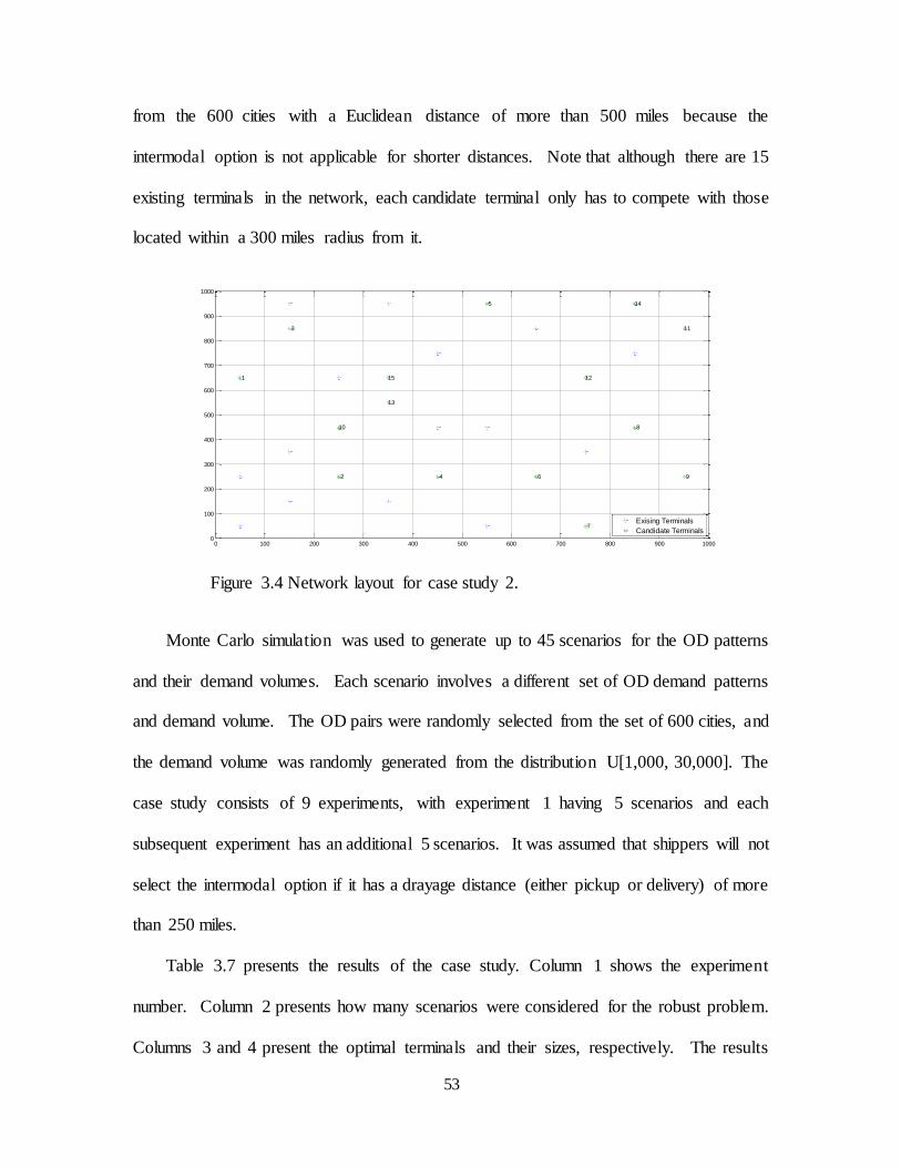
53

from the 600 cities with a Euclidean distance of more than 500 miles because the

intermodal option is not applicable for shorter distances. Note that although there are 15

existing terminals in the network, each candidate terminal only has to compete with those

located within a 300 miles radius from it.

Figure 3.4 Network layout for case study 2.

Monte Carlo simulation was used to generate up to 45 scenarios for the OD patterns

and their demand volumes. Each scenario involves a different set of OD demand patterns

and demand volume. The OD pairs were randomly selected from the set of 600 cities, and

the demand volume was randomly generated from the distribution U[1,000, 30,000]. The

case study consists of 9 experiments, with experiment 1 having 5 scenarios and each

subsequent experiment has an additional 5 scenarios. It was assumed that shippers will not

select the intermodal option if it has a drayage distance (either pickup or delivery) of more

than 250 miles.

Table 3.7 presents the results of the case study. Column 1 shows the experiment

number. Column 2 presents how many scenarios were considered for the robust problem.

Columns 3 and 4 present the optimal terminals and their sizes, respectively. The results

0 100 200 300 400 500 600 700 800 900 10000

100

200

300

400

500

600

700

800

900

1000

1

2

3

4

5

6

7

8

9

10

11

12

13

14

15

Exising Terminals

Candidate Terminals

54

show that locations 9 and 11 were never selected because they are located in isolated areas

of the network. Since they both have a much smaller market, it would not be profitable to

open new terminals at these locations. On the other hand, locations 4, 7, 8, 10 and 15 were

included in the optimal set in more than 50% of the experiments. Due to the randomness

in OD patterns, the decision of where to locate new terminals is more complicated than

when the OD patterns do not change. The results indicate that as the number of scenarios

increases, the results of the robust model becomes more consistent. It be can be seen in

Table 3.7 that as the number of scenarios gets higher, the solutions converge to a set of

similar candidate locations. Specifically, it indicates that regardless of the scenario,

candidate terminals 4, 7, 10 and 15 should be selected. An interesting observation from

this case study is that the optimal locations could be identified using a smaller set of

scenarios, but the optimal throughput capacities will need to use a much larger set of

scenarios. In reality, it is unlikely to have scenarios where the OD demand patterns and

demand volume differ drastically. Thus, it is expected that the developed robust model

will be able to identify both optimal locations and terminal sizes using a relatively small

number of scenarios.

Table 3.7 Solution of the robust model P1 for case study 2.

Experiment

#

# of

scenarios

Selected

terminals Throughput capacity (TEU)

1 5 7, 10, 14 8,408,300;4,445,800;7,434,700

2 10 1, 4, 7, 10, 15 4,872,100; 2,817,200; 7,779,800; 5,130,000; 441,300

3 15 1, 6, 10, 14, 15 625,199; 7,735,600; 3,596,500; 6,790,600; 3,813,900

4 20 3, 4, 7, 8, 12 6,898,000; 4,335,000; 7,472,000; 15,674,000; 799,400

5 25 5, 8, 10, 12, 15 15,008,000; 73,300,000; 4,576,000; 7,224,000; 5,156,000

6 30 2, 7, 8, 10, 15 3,482,000; 8,353,000; 15,369,000; 4,119,000; 5,344,000

7 35 3, 4, 7, 8, 12 7,430,000; 4,469,000; 15,616,000; 7,961,000; 7,812,000

8 40 4, 7, 8, 10, 15 5,759,000; 15,224,000; 8,557,000; 5,436,000; 4,985,000

9 45 4, 7, 10, 13, 15 15,325,000; 15,623,000; 4,225,000; 3,481,000; 3,276,000

55

3.6 MANEGERIAL IMPLICATIONS

To gain insights on the implications of different managerial actions, two additiona l

situations were analyzed. The first involves investigating the sensitivity of drayage

distance on a terminal’s ability to capture market share, and the second involves

investigating the managerial option of closing an existing terminal and opening 1 or 2 new

terminals at the candidate locations. The analysis was applied using the same network used

for case study 1 and the 2040 FAF3 predicted freight flow for South Carolina.

In the proposed model, shipments going from i to j are allocated to terminals (k, m)

based on their utility. The longer the drayage distances, from origin i to terminal k and

from terminal m to destination k, the less attractive the terminal pair (k, m) is to shippers.

To test the sensitivity of drayage distance on a terminal’s ability to capture market share,

we analyzed scenarios where shippers have a threshold on the maximum drayage distance

they are willing to consider. In other words, we considered scenarios where shippers will

only consider a terminal pair if their resulting drayage distances is less than their desired

threshold. From the modeling standpoint, we effectively set the utility of terminals (k, m)

to 0 if its drayage distances exceed the threshold. Table 3.8 presents the results of this

analysis. Column 1 shows the different drayage distance thresholds considered. Column 2

shows how many new terminals will be opened. Columns 3 and 4 present the company’s

intermodal share and the competitor’s intermodal share, respectively. Column 5 shows the

remaining percentage of shipments using the truck-only option. The last column shows the

obtained best locations for new terminals.

56

Table 3.8 Effect of drayage distance thresholds on intermodal market shares and locations

Drayage

Distance

threshold

(miles)

# of new

terminals

Own

company’s

intermodal

share

Competitor’s

intermodal

share

Truck only

modal

share

Selected terminals

100

1 27% 19% 54% Greenville

2 33% 18% 49% Greenville,

Florence

3 35% 18% 47% Greenville,

Florence, Augusta

4 37% 17% 46% All

250

1 50% 30% 20% Lexington

2 53% 27% 20% Lexington,

Augusta

3 56% 24% 20%

Lexington,

Augusta,

Greenville

4 59% 22% 19% All

350

1 50% 31% 19% Lexington

2 53% 28% 19% Augusta,

Lexington

3 56% 26% 18%

Lexington,

Augusta,

Greenville

4 58% 24% 18% All

500

1 51% 31% 18% Augusta

2 54% 29% 17% Augusta,

Lexington

3 56% 27% 17%

Florence,

Augusta,

Lexington

4 58% 25% 17% All

It can be seen in Table 3.8 that when the drayage threshold is low (i.e. 100 miles), the

truck uni-mode is generally preferred over intermodal. This is because the lower the

threshold, the fewer opportunities there are for the intermodal option. In scenarios which

have a higher number of new terminals, the railroad company has a better chance to

increase its market share. The results indicate that when the drayage distance threshold

ranges from 250 to 500, there is little difference in market share for intermodal and truck

uni-mode. However, increasing the number of new terminals will increase the market share

57

for the railroad company. It is also worth mentioning that different drayage distance

thresholds affect the optimal location selection. As shown in Table 3.8, Greenville is the

optimal terminal location when there is 1 new terminal and the drayage distance threshold

is 100 miles, but Lexington becomes the optimal location when the drayage distance

threshold is 250 and 350 miles. Thus, an important design consideration in determining

the optimal locations is the shippers’ drayage distance threshold. Such information could

be easily obtained via survey and be incorporated into the model.

Typically, a railroad company would expand its network by opening new termina ls.

Another option the manager may want to consider is closing an existing terminal which is

not attracting enough demand and opening new terminals in more attractive locations.

Such a situation was investigated. Two sets of experiments were conducted. The first

involves closing one existing terminal and opening one new terminal, and the second one

involves closing one existing terminal and opening two new terminals. The base case (BC)

scenario for the first set of experiments involves closing no existing terminal and opening

no new terminal, and the BC for the second set of experiments involves closing no existing

terminal and opening one new terminal. The results shown in Figure 3.5 indicate that by

closing any of the existing terminals at the indicated locations (see x-axis labels) and

opening 1 or 2 new terminals, the railroad company will gain market share compared to

the base case. The only exception is Charleston. Note that the market share when closing

the Charleston terminal is 49.2 % compared to 49.9% of the BC. Closing the termina l

located in Atlanta has the highest impact on market share for both cases (opening 1 or 2

new terminals). This result suggests that Atlanta terminal is the least attractive termina l

among the existing terminals. It should be noted that the greatest increase in the total

58

market share is about 3% (scenario involving closing the Atlanta terminal and opening one

new terminal). Thus, the manager will need to conduct a benefit-cost analysis to determine

whether it is beneficial to close an existing terminal and open a new one.

Figure 3.5 Change in market share by closing one existing terminal and opening new terminals.

3.7 CONCLUSIONS

This paper developed a mixed integer nonlinear programming model to find the best

locations for new intermodal terminals and their capacities in a competitive environment

with uncertain demand. Robust optimization models with min-max regret and minimum

expected regret criteria were used to find solutions which are near optimal for any

realization of demand scenarios. A simulated annealing algorithm was developed to solve

the developed models. Computational experiments showed that the developed SA

algorithm was able to find solutions with 0% gap compared to GAMS solutions, but in

much shorter time for midsize problems. Moreover, the developed SA algorithm was able

to solve larger-sized problems that GAMS could not (on a computer with 8 GB of RAM).

BC Savannah1 Savannah2 Atlanta Charlotte Charleston44

45

46

47

48

49

50

51

52

Location of Existing Terminal to be Closed

Mark

et S

hare

Perc

enta

ge

opening 1 new terminal

opening 2 new terminals

59

The results verified that location and capacity decision is more robust when considering

different scenarios of freight demands.

This work contributed to the literature of intermodal terminal location problem by

considering competition between existing terminals and new terminals, terminal capacity,

and uncertainty in freight demands. In future work, there are several potential areas for

improvement. In the area of competition, it could be enhanced by considering utility

functions based on transportation rates and multi-period travel times. In the area of

terminal capacity, it could be enhanced by considering capacity expansion for existing

terminals based on predicted freight demands. Lastly, it could be enhanced by utilizing

fuzzy or stochastic approaches to deal with uncertainty in freight demands.

While the proposed model and solution approach have been validated via case studies,

key limitations should be considered when reviewing study results. These included: 1)

choice of network topology and size, 2) accuracy of FAF3 predicted freight flows, 3)

design of the scenarios and experiments, and 4) objective of the optimization model that

considers only profit from the new terminal.

60

CHAPTER 4: RELIABLE INTERMODAL FREIGHT NETWORK EXPANSION WITH DEMAND UNCERTAINITIES AND NETWORK

DISRUPTIONS2

2 Fotuhi. F and Huynh. N. Networks and Spatial Economics , 2016, pp. 1-29. Reprinted here with

permission of publisher

61

ABSTRACT

This paper develops a robust Mixed-Integer Linear Program (MILP) to assist railroad

operators with intermodal network expansion decisions. Specifically, the objective of the

model is to identify critical rail links to retrofit, locations to establish new terminals, and

existing terminals to expand, where the intermodal freight network is subject to demand

and supply uncertainties. Additional considerations by the model include a finite overall

budget for investment, limited capacities on network links and at intermodal terminals, and

time window constraints for shipments. A hybrid Genetic Algorithm (GA) is developed to

solve the proposed MILP. It utilizes a column generation algorithm to solve the freight

flow assignment problem and a multi-modal shortest path label-setting algorithm to solve

the pricing sub-problems. An exact exhaustive enumeration method is used to validate the

GA results. Experimental results indicate that the developed algorithm is capable of

producing optimal solutions efficiently for small-sized intermodal freight networks. The

impact of uncertainty on network configuration is discussed for a larger-sized case study.

4.1 INTRODUCTION

A robust freight transport system is a key contributor to the success of the U.S. economy

(Ortiz et al., 2007). However, the existing freight transport system is running at its capacity

due to increase of trades and an aging infrastructure. Thus, it has a limited buffer to handle

the severe disruptions (Ortiz et al., 2007). Disruptions can range from frequent events with

short term impacts, such as adverse weather, accidents and loading/unloading delays at

intermodal terminals, to catastrophic natural and man-made disasters with long term

impacts which can drastically degrade the transport capacity (Ortiz et al., 2007; Miller -

Hooks et al., 2012). Examples of catastrophic disasters with long term impacts are

62

Hurricane Katrina, which damaged the transportation infrastructure of Gulf Coast area

(Godoy, 2007) and the West Coast port labor strike which disrupted the U.S. freight supply

chain (D’Amico, 2002). Thus, in order for the freight transport system to be able to handle

such disruptions, there is a need to increase its capacity by incorporating redundant

resources and backup facilities, and retrofitting existing infrastructure (Peeta et al., 2010;

Liu et al., 2009).

Intermodal network design is a strategic level planning problem which finds the

location of intermodal terminals and assignment of freight flow to the network. Strategic

planning decisions deal with network infrastructure creation or expansion (SteadieSeifi,

2014). SteadieSeifi et al. (2014) recently provided a comprehensive overview of models

and algorithms developed for strategic, tactical and operational multi-modal freight

transport planning problems. According to this review, most strategic studies neglected

two important practical aspects. The first is that the design does not consider existing

intermodal infrastructure, which is not realistic in practice. It is more realistic to expand

an existing freight transport network rather than designing a system from scratch (Gelareh

et al., 2010). The second is that prior strategic studies neglected the possible changes in

demand and supply that may occur over the planning period. Demand changes are to be

expected as a result of pricing and supply changes over time, as well as the influx of new

users in the system (Melese et al., 2016). Also, as new terminals come online, demands

and freight flow patterns may be very different from what was envisioned at the network

design phase (Taner and Kara, 2015). This research seeks to fill these gaps by developing

a mathematical model to address expansion of an existing intermodal freight network and

making it reliable; reliability means that the network can continue delivering service when

63

faced with shocks, such as influx in freight demands or disasters that reduce capacity of

network links and intermodal terminals.

This study deals with a rail-road intermodal network expansion problem for a private

rail carrier that is responsible for its own maintenance and improvement projects, typical

of U.S. Class 1 railroads. The strategic decision involves identifying locations for the new

intermodal terminals, expanding the existing terminals and retrofitting the existing rail

links in the network to enhance its survivability, given a finite budget. The strategic

decision will subsequently affect the operational decision concerning freight flow

assignment through the network. Thus, the routing decision is factored in the investment

decision in the proposed model. A robust optimization approach is utilized to account for

forecast demand errors and potential supply disruptions. The optimal decision seeks to

minimize the total expansion, transport and lost-sale costs of the railroad company; lost-

sale cost is incurred to the railroad company when it fails to deliver shipments on time.

The rest of the paper is organized as follows. Section 2 provides a summary of related

studies. Section 3 presents the developed mathematical model. Section 4 discusses the

proposed solution algorithm to solve the model. Section 5 discusses the results of the

numerical experiments. Lastly, Section 6 provides concluding remarks and future research.

4.2 LITERATURE REVIEW AND BACKGROUND

4.2.1 LITERATURE REVIEW

Intermodal network design has become an emerging body of research within the

transportation field (Bontekoning et al., 2004). In an intermodal network, smaller

shipments are collected and consolidated at distribution centers. Then, all consolidated

shipments are loaded into containers and shipped to the intermodal terminals with trucks.

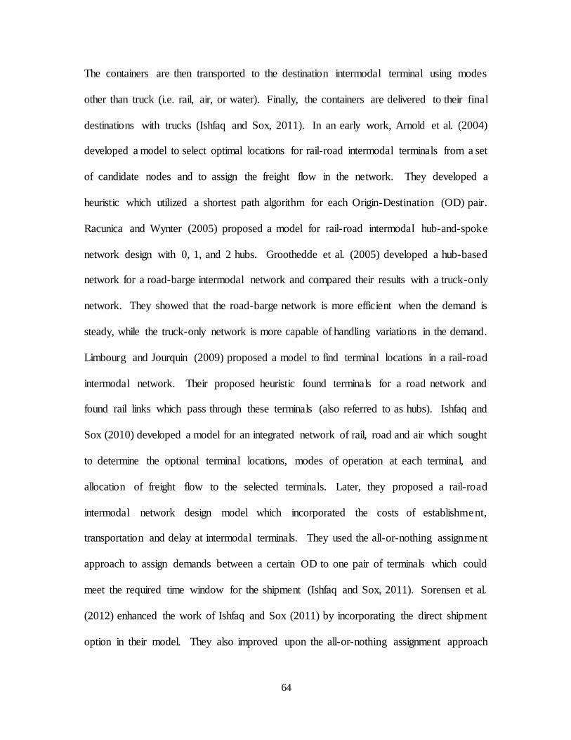
64

The containers are then transported to the destination intermodal terminal using modes

other than truck (i.e. rail, air, or water). Finally, the containers are delivered to their final

destinations with trucks (Ishfaq and Sox, 2011). In an early work, Arnold et al. (2004)

developed a model to select optimal locations for rail-road intermodal terminals from a set

of candidate nodes and to assign the freight flow in the network. They developed a

heuristic which utilized a shortest path algorithm for each Origin-Destination (OD) pair.

Racunica and Wynter (2005) proposed a model for rail-road intermodal hub-and-spoke

network design with 0, 1, and 2 hubs. Groothedde et al. (2005) developed a hub-based

network for a road-barge intermodal network and compared their results with a truck-only

network. They showed that the road-barge network is more efficient when the demand is

steady, while the truck-only network is more capable of handling variations in the demand.

Limbourg and Jourquin (2009) proposed a model to find terminal locations in a rail-road

intermodal network. Their proposed heuristic found terminals for a road network and

found rail links which pass through these terminals (also referred to as hubs). Ishfaq and

Sox (2010) developed a model for an integrated network of rail, road and air which sought

to determine the optional terminal locations, modes of operation at each terminal, and

allocation of freight flow to the selected terminals. Later, they proposed a rail-road

intermodal network design model which incorporated the costs of establishment,

transportation and delay at intermodal terminals. They used the all-or-nothing assignment

approach to assign demands between a certain OD to one pair of terminals which could

meet the required time window for the shipment (Ishfaq and Sox, 2011). Sorensen et al.

(2012) enhanced the work of Ishfaq and Sox (2011) by incorporating the direct shipment

option in their model. They also improved upon the all-or-nothing assignment approach

65

by enabling the model to assign different fractions of shipments for an OD pair to truck-

only or rail-road intermodal option. Vidovic et al. (2011) proposed a model to find optimal

locations for intermodal terminals by considering the hub catchment area. They assumed

that each terminal will attract the demand within a specific radius from it. They used

simulation to come up with freight demand due to the limited real world freight data.

Fotuhi and Huynh (2013) developed an intermodal model that considered more than two

modes of transport. Their model jointly selected terminal location, shipping modes and

optimal routes for shipping different types of commodities. Peker et al. (2015) proposed a

data-driven approach to find optimal locations for transportation hubs based on demand

density and spatial features of potential hubs. They used a clustering-based heuristic to

find the optimal locations. Recently, Meng and Wang (2011) proposed a model for

expanding an intermodal network and taking the existing infrastructure into account. They

proposed a model to optimally expand existing links and transshipment lines, as well as

establishment of new hubs and links given a limited budget, while minimizing the total

transportation and expansion costs. Their work is the first study to address the intermoda l

network expansion problem. Fotuhi and Huynh (2015) proposed a model to find locations

for new intermodal terminals by considering terminal’s catchment areas, uncertain demand

and competition in the network. In their study a private intermodal service provider

assumed to expand its network and intend to attract more demand from a competing

company that has overlapping service areas with it.

The aforementioned works did not consider the possibility of failures in network

elements. However, the occurrence of natural or man-made disasters in any transportation

network is inevitable. A number of researchers have studied vulnerability of uni-moda l

66

transportation networks where a disaster could significantly reduce the capability of

network to meet the demands. Berdica (2002) studied a vulnerable road network as a

system that is sensitive to disruptions which could cause significant reduction in

accessibility and disturbances of traffic. D'Este and Taylor (2003) noted that it is important

to identify and strengthen the weakest elements of a network to decrease its vulnerability.

This is feasible by including reliability criteria in the network design decisions, such as

what investments to make to strengthen the network pre-disaster and what investments

needed to enhance post-disaster recovery (Dayanim, 1991).

In recent years, there is a growing body of work that addresses disruptions in the

context of network design. Almost all of these studies considered uni-modal transportation

networks with risk of link failures. In an earlier work, Rios et al. (2000) studied a

capacitated network design problem with arc failure risk. Their model determined which

set of links to open and determined their capacities so that the network survives disruptions,

with the goal of fixed costs minimization. Viswanath and Peeta (2003) proposed a mult i-

commodity maximal covering network design model for identifying critical routes and

retrofitting bridges on these routes within a limited budget for earthquake response. Garg

and Smith (2008) formulated a survivable multi-commodity network design model with

arc failures to determine which arcs to construct so that the network survives the future

disruptions. In a more general work, Desai and Sen (2010) formulated a reliable network

design model with arc failure risks which minimized network design costs as well as

resource allocation cost of mitigating higher risk arcs. A few researchers have studied the

retrofitting decision for the existing links of a network. These studies deal with the tactical

planning problem of optimally using the existing infrastructure (SteadieSeifi et al., 2014).

67

Liu et al. (2009) developed a model to allocate limited budget to retrofit more critical

bridges in a network. They assumed that if a bridge is retrofitted, it would not collapse in

case of disasters. Peeta et al. (2010) also proposed a pre-disaster investment model to

retrofit more critical links in a highway network.

Disruptions may also affect facilities in a network. Snyder and Daskin (2005) were

among the first to study the reliable p-median and uncapacitated facility location problems

with facility failures. Their models sought to find location of warehouses to minimize

transportation cost in normal situations and expected failure cost in disrupted situations.

They assumed that unreliable facilities have the same failure probability. Cui et al. (2010)

relaxed the identical failure probability assumption in Snyder and Daskin (2005) and

considered facility–dependent failure probabilities in their model. Shishebori et al. (2014)

proposed a model for combined facility location and network design problem by

considering system reliability. They assumed that failures only happen in network nodes.

However, their model decided which facilities to open and which links to construct to

compensate for disruptions. The risk of facility failures have also been addressed in the

context of logistics and transportation network design. Peng et al. (2011) developed a

reliable logistic network design model with supplier and distribution center failures. Hatefi

and Jolai (2014) developed a reliable forward-reverse logistics network model with

distribution center failure risk. They considered uncertain demand as well as possible

disruptions in their model. An et al. (2011) developed a hub network design model with

hub failures. Unlike previously mentioned studies, disrupted facilities in this work were

transshipment nodes. Their model identified hubs that can serve as backup hubs for

disrupted situations. Their model’s objective sought to minimize the expected cost of

68

routing all flows in normal situations as well as disrupted situations. Marufuzzaman et al.

(2014) developed a model for biofuel supply chain design with intermodal termina l

disruptions. Their model’s objective was to find locations for intermodal terminals and

bio-refineries while minimizing total establishment and transportation costs. The Miller-

Hooks et al. (2012) study is the only prior work that considers disruptions of both links and

nodes in a transportation network. They developed a stochastic two-stage model to allocate

limited budget to improve the resiliency of an intermodal network by choosing a set of pre-

disaster and recovery activities. This is a tactical planning model which aimed to improve

the existing infrastructure.

This work extends the work of Meng and Wang (2011) by considering uncertainty in

both demand and supply. Additionally, it combines the tactical planning retrofitt ing

decisions addressed by Miller-Hooks et al. (2012) with the strategic planning decision.

This is the first study to jointly address tactical and strategic decisions in the context of

intermodal network resiliency. In summary, this work contributes to the literature of

intermodal network design and expansion by including demand and supply uncertaint ies

and incorporating retrofitting decisions in the design phase. As such, these are its technical

contributions.

1. A new model for the intermodal freight network expansion problem that jointly

considers strategic network decisions, tactical retrofitting decisions, and

operational freight flow assignment.

2. A robust and reliable model for intermodal network design/expansion, which

simultaneously takes into account uncertain freight demands and infrastruc ture

disruptions.

69

3. A hybrid genetic algorithm that is capable of solving the proposed model for

realistic-sized networks in a reasonable amount of time. A modified version of the

well-known label setting algorithm is proposed to consider problem-specific

constraints for routing decisions.

4.2.2 BACKGROUND (ROBUST OPTIMIZATION)

Robust Optimization (RO) is an approach to modeling optimization problems under

uncertainty. Rather than treating the problem as stochastic, RO treats the problem as

deterministic and set-based. That is, instead of seeking an optimal solution in some

probabilistic sense, RO constructs a solution that is feasible for any realization of the

uncertainty in a given set. The motivation for this approach is twofold. First, in many

applications a set-based approach is appropriate for capturing parameter uncertainty.

Second, RO makes the problem computational tractable.

One of the more common approaches in RO is min-max regret which was first

developed by Kouvelis and Yu (1997). It finds the solution with less distance from the

optimal values of all scenarios. This distance is called regret that is the loss incurred for

not choosing the optimal design for each scenario. This criterion is suitable in situations

where the decision maker may feel “regret” if he/she makes a wrong decision. Thus, he/she

thus takes this anticipated regret into account when deciding a solution. For example, in

finance, an investor may have the opportunity to invest in a number of portfolios. Under

the min-max regret approach, he/she would choose a portfolio that minimizes the

maximum difference between his/her portfolio’s performance and that of other portfolios.

In some situations, the min-max criteria is too pessimistic for those decision makers who

are willing to accept some degree of risk because its solution is affected by the worst case

70

scenarios which are sometimes unlikely to occur. However, this issue could be addressed

at the modelling stage by including only relevant scenarios in the scenario set. The reader

may refer to the work of Ben-Tal and Nemirovski (2002) and Bertsimas et al. (2011) for

more information about robust optimization. The followings are basic principles of min-

max regret.

Let S represent a set of s finite scenarios for an uncertain parameter (e.g. demand, link

capacity) and x denote a feasible solution for the robust problem. )(xOs is the objective

function value of scenario s at feasible point x and *sO is the optimal solution for scenario

s (for all x in the set X). Regret is represented by the difference between )(xOs and *

sO .

The min-max regret obtains a solution which minimizes the maximum regret over all

scenarios and is formulated as follows.

)))((( *

ssSsXx

OxOMaxMin

(4.1)

A few studies in the literature have used the min-max regret approach for facility

location and supply chain design problems (e.g., Daskin et al., 1997; Ramezani et al.,

2013). To our knowledge, this is the first study to apply robust optimization to the

intermodal network design and expansion problem.

4.3 MODELING FRAMEWORK

This section presents the formulation of the model that addresses the rail-road intermoda l

network expansion with network disruptions and demand variations. This model extends

the classical intermodal network design problem by considering existing infrastructure. As

explained previously, its goal is to identify locations for new intermodal terminals, existing

terminals to expand, and rail links to retrofit so that the total transportation cost and lost-

sales cost is minimized for normal and disrupted situations.

71

Consider a railroad company which intends to expand its intermodal network. The

network representation for this company is given by ),( ANG , where N is the set of nodes

and A is the set of arcs. G consists of sub-networks, ),( 11 ANG and ),( 22 ANG for road and

rail networks, respectively. Transfer between modes takes place at intermodal termina ls.

1N represents cities, and 2N represents intermodal terminals in the rail network.

2N

includes existing terminals (3N ) and candidate terminals (

4N ). 1A and

2A represent

highway and rail arcs, respectively. The network enables freight shipments to be

transported between OD pairs represented by W either by truck-only or intermodal. A set

of paths wP comprising a chain of arcs is given for each OD pair Ww . The travel time

for an intermodal path is computed using the individual links’ travel times and transfer

times at intermodal terminals. Note that some paths might be infeasible due to time

window constraints or because they include candidate terminals that have not been selected

to be built.

The proposed model makes the following assumptions: (1) the expanded intermoda l

terminals, the newly established terminals, and the retrofitted rail links are able to withstand

disruptions, (2) shipments with late delivery are considered as lost-demand and incur a

penalty cost, (3) if the shortest path cost for a shipment is higher than the penalty cost for

lost-demand, the shipment is considered as an unmet-demand, and (4) there is no delay for

shipments passing through an intermodal terminal that do not require a changing of mode.

It is assumed that a few expansion designs jj Ll with a given cost of jlj

C,

and capacity

of jljv ,

are available for existing terminals 3Nj . jlj

C,

denotes the cost for labor,

equipment, and storage space to handle additional jljv ,

containers. S is a set of scenarios,

72

each of which represents a normal or disrupted situation. Other parameters used in the

formulation of the Reliable Intermodal Network Expansion Problem (RINEP) include:

Parameters

at : travel time on link a

j : transfer time at intermodal terminal j

wT : delivery due date for OD pair w

ae : capacity of link a

j : capacity of intermodal terminal j

sa : disruption percentage for link a under scenario s

sj : disruption percentage for terminal j under scenario s

B : available budget for investment decisions

swd : demand of OD pair w under scenario s

jF : fixed cost of opening a new terminal at location j

ah : retrofitting cost for rail link a

wak : path-arc incidence (= 1 if link a is used in path k for OD pair w; 0 otherwise)

wjk : path-terminal incidence (=1 if shipments change mode at terminal j in path k for

OD pair w; 0 otherwise)

The decision variables are as follows.

Strategic and Tactical Decision Variables

Otherwise0

;locationat opend is terminala If1 4Ny

jj

Otherwise0

d;retroffite islink If1 2Az

aa

73

Otherwise 0

terminalexistingfor selected is design expansion If1 ;' 3

,

Nlv

jj

jlj

Once the strategic and tactical decision variables are determined, the freight flow is

assigned to the network. The flow assignment step considers the following decision

variables which are scenario dependent.

Otherwise 0

; scenarioin path uses pair D If1 skwOwskx

skwwskf scenariofor path on pair ODfor flowfreight ofAmount :

RINEP Formulation

ZMinimize (4.2)

Subject to:

SsZOcfhzCvyF s

wk

kws

k

Nj Nj Aa

aaljljjj jj

,)'( *

,

,,

4 3 2

(4.3)

SsNjvvvfjj ljljj

s

j

kw

w

jk

ws

k ,,)1( 3,,

,

(4.4)

SsNjvf j

kw

w

jk

ws

k ,, 4

,

(4.5)

BhzCvyFNj Nj Aa

aaljljjj jj

4 3 2

,,' (4.6)

3, ,1' Njvj

j

l

lj (4.7)

SsAaefkw

a

s

a

w

ak

ws

k ,,)1( 1

,

(4.8)

SsAaezfkw

aa

s

a

w

ak

ws

k ,,))1(1( 2

,

(4.9)

SsPkWwxMT

tzt

w

ws

kw

Nj

w

jkj

Nj

w

jkj

s

j

w

aka

Aa

a

s

a

w

aka

Aa

s

a

,,),1(

))(1())1(1()1(4321

(4.10)

74

SsWwPkMxf w

ws

k

ws

k ,,, (4.11)

SsNjMyx j

w

jk

kw

ws

k ,, 4

,

(4.12)

SsWwdf s

w

k

ws

k ,, (4.13)

SsNjAaWwfxvzy ws

k

ws

kljaj j ,,,,0},1,0{,,, 22

'

, (4.14)

The objective function (4.2) minimizes the maximum regret over all scenarios.

Constraints (4.3) ensure that the regret for each scenario is greater than the minimum regret.

Constraints (4.4) and (4.5) guarantee that the capacity of existing and new terminals are

not violated, respectively. Constraint (4.6) ensures the amount of money used for

establishment of new terminals, expansion of existing terminals, and retrofitting of rail

links is within the available budget B. Constraints (4.7) ensure that at most one expansion

design can be selected for existing terminals. Constraints (4.8) and (4.9) prevent highway

and rail link capacities from being exceeded. Constraints (4.10) assign flows to the paths

to meet delivery due dates. These constraints only hold if path k is used for OD pair w.

Constraints (4.11) and (4.12) ensure that flows are assigned to selected paths and open

terminals, respectively. Constraints (4.13) ensure that the total flow shipped over all

feasible paths between an OD pair equals to the demand for this OD pair. Constraints

(4.14) impose non-negativity and integrality on the decision variables. A Determinis t ic

Intermodal Network Expansion Problem (DINEP) is used to obtain *

sO for scenario s which

can be expressed as follows.

DINEP:

wk

k

ws

k

Nj Nj Aa

aaljljjjs cfhzCvyFMinimizeOjj

,

,,

*

4 3 2

' (4.15)

75

s.t.: (4.4)-(4.14)

The objective function (4.15) minimizes the total cost, which consists of the cost of

opening new terminals, cost of expanding existing terminals, cost of retrofitting rail links,

and transport cost.

4.4 SOLUTION METHOD

RINEP and DINEP are both classes of the discrete network design problem which is NP-

hard (Meng and Wang, 2011). A few researchers have developed algorithms based on

Lagrangian relaxation and Benders decomposition to solve the robust network design

problems (Miller-Hooks et al., 2012; Snyder and Daskin, 2006a). These algorithms

provide exact solutions; however, as the number of scenarios and network size increase the

algorithm become less efficient. For larger-sized problems, it may take several days to

find a feasible solution, with no optimality guaranteed (Miller-Hooks et al., 2012). In this

paper, a new algorithm is proposed in an effort to identify more efficient solution

algorithms for this class of problems. The proposed algorithm uses GA which has been

widely implemented due to its ability to find optimal or near-optimal solutions for large-

sized problems (Holland, 1975). Recently, a few researchers have used GA to solve the

bi-level network design problems (Meng and Wang, 2011; Peng et al., 2011; Ko and Evans,

2007). In these papers, the strategic planning variables were first determined by GA, and

subsequently the corresponding transportation sub-problems were solved using the

problem-specific algorithms. A similar approach is adopted in this paper.

The proposed algorithm incorporates GA and the Column Generation (CG) method.

The GA component is used to find values for the strategic decision variables. Once the

values for these variables are determined, the flows are assigned to the network by solving

76

a Capacitated Multi-Commodity Intermodal Network Flow Problem with Time Windows

(CMCINFPTW) for scenario s to find *sO . The CG method is used to solve the

CMCINFPTW. For the robust problem, S CMCINFPTW are solved to find sO . There

are some differences in the GA component for solving RINEP and DINEP; these details

are provided in subsequent sections.

4.4.1 CHROMOSOME REPRESENTATION

The proposed GA comprises a three-part chromosome with binary and integer genes to

represent the strategic planning variables. The first part represents the set of candidate

terminals to open. The second part represents the rail links to retrofit, and the last part

represents the existing terminals to expand. Figure 4.1 illustrates the chromosome

representation for a solution. As shown, this chromosome indicates that the problem deals

with 3 candidate locations for new terminals, 8 rail links to be considered for retrofitt ing,

and 3 existing terminals to be considered for expansion. The first part of the chromosome

indicates that among the 3 potential locations, a new terminal should be opened at location

2 (=1). The second part of the chromosome indicates that rail links 3 and 8 should be

retrofitted (=1). The last part of the chromosome indicates that expansion designs 2, 1, and

3 should be selected for the three existing terminals, respectively.

Note that in the formulation, binary variables are used to determine which expansion

design to select for an existing terminal. Thus, an existing terminal with m available

designs needs m binary genes. To reduce the number of genes in the chromosome, each

gene in third part of chromosome stores an integer value rather than a binary value. The

integer value denotes the expansion design to select for the existing terminal. Using this

representation, for the example illustrated in Figure 4.1, the number of genes in the third

77

part of the chromosome is reduced from 9 (3 terminals x 3 possible expansion designs) to

3.

Figure 4.1 Chromosome representation

4.4.2 INITIAL POPULATION GENERATION

Alander (1992) suggested that an appropriate population size for a problem with n decision

variables in a chromosome is between n and 2n. Preliminary experiments were conducted

over this range (n to 2n) and the results indicated that an initial population size of n is

sufficient. For the robust model (RINEP), the initial population is generated by includ ing

the optimal chromosomes of each scenario which are obtained by optimally solving DINEP

for each scenario separately. If the number of scenarios is more than n, then n scenarios

are randomly considered for the initial population. If the number of scenarios is less than

n, additional chromosomes are generated by using crossover and mutation operators to

make the initial population size to be n. Chromosomes (i.e. solutions) that violate the

budget constraint are discarded from a population.

4.4.3 GA OPERATORS

Roulette wheel selection and tournament selection are the two most common GA selection

methods. In this study, the binary tournament selection method is used instead because it

has been shown to generate better solutions for the class of problems considered in this

study (Chu and Beasley, 1997). Preliminary experiments tested several crossover

operators, including one-point crossover, two-point crossover, uniform crossover, and

0 1 0 0 0 1 0 0 0 0 1 2 1 3

Part 1 Part 2 Part 3

78

multipoint crossover. The two-point crossover with 0.8 crossover probability was found

to generate better solutions and thus adopted in our solution approach. The mutation

operation used in this study is that the binary genes have a probability of 0.1 to change

from 1 to 0 or vice-versa and integer genes (in part 3 of chromosome) have equal

probability of taking on a value from 0 to the number of available expansion designs.

4.4.4 FITNESS FUNCTION

The fitness value (i.e. the objective function value) can be determined given a chromosome

(solution). In this study, the fitness value for RINEP and DINEP are computed using

objective functions (4.2) and (4.15), respectively. Specifically, after obtaining a solution

for the strategic problem ),,( zvy , |S| CMCINFPTW are solved with CG to find flow

assignment for demands between each OD pair. Once all the flows are determined, sO can

be computed using Equation (4.15) and regret values can be computed for each scenario

using Equation (4.2).

As mentioned previously, by fixing the design variables ),,( zvy , DINEP becomes

CMCINFPTW. The CMCINFPTW finds the least cost paths for each OD pair such that

the capacity of the arcs and intermodal terminals are not exceeded and no delivery delay is

incurred. If no such path can be found, a penalty cost is incurred. This is accomplished by

assuming that in the network there exists a hypothetical path between the origin and

destination for the shipment, and that the path has infinite capacity and instantaneous travel

time (Peng et al., 2011). The cost of the hypothetical path is set to be the penalty cost for

each unit of unmet demand.

CMCINFPTW is a class of the well-known Capacitated Multi-Commodity Network

Flow Problem (CMNFP) with additional constraints. CMNFP is NP-hard but can be

79

solved by CG (Ahuja et al., 1993; Yaghini et al., 2012). CG incorporates a master problem

which finds the optimal objective value by considering a portion of decision variables as

basic variables and a pricing problem to find decision variables that can improve the

objective function if they enter the basis. This study adapts the CG method proposed by

Ahuja et al. (1993) to solve the CMCINFPTW for each scenario. Ahuja et al. (1993) stated

that the pricing problem for CMNFP is a constrained shortest path problem; one for each

OD pair which can be solved using the well-known label-setting algorithm from mult i-

period programming. Hence, an intermodal label-setting algorithm is proposed in this

paper to solve CMCINFPTW.

4.4.4.1 INTERMODAL LABEL SETTING ALGORITHM

Cho et al. (2012) was among the first to propose a label setting algorithm for a mult i-

objective intermodal routing problem with time windows. Their algorithm sought to find

the route with the minimum total cost and minimum travel time. It attached a label to each

node which included travel time as a constraint and travel cost as the objective function.

This study adapts their algorithm by adding “capacity” and “mode” to the label to enable

the modeling of network disruptions as well as consideration of the transfer time and

transfer cost at intermodal terminals. “Capacity” is used to check for possible disruptions

of network elements (link or node). If the network element is not functional, then the label

would contain a value of zero for capacity. “Mode” is used to determine if there is a change

of mode at an intermodal terminal. If so, then the transfer time and transfer cost at the

intermodal terminal are added to the path’s cost and time. Nodes with a capacity of zero

and/or a transfer time that leads to a violation of the time window constraints are eliminated

from further consideration in the algorithm.

80

4.4.5 TERMINATION CRITERIA

A maximum of 100 (Num_G) generations is used as a termination criterion for the GA.

The algorithm also terminates if it cannot improve the objective function value for 10 (k)

consecutive generations. The key algorithmic steps are presented below.

Step 0: Set 0,0 kt

Step 1: Randomly generate n distinct chromosomes satisfying budget constraint. Compute

fitness value for each chromosome. Let )( ,, ttt zvy be the best chromosome in the

population; let )( **,*, zvy be the incumbent solution (i.e., 0)( **,*, zvy ).

Step 2: If *)*,*,(),,( zvyfzvyf ttt , then set ),,(*)*,*,( ttt zvyzvy .

Step 3: Make a new generation by performing a two-point crossover with a probability of

cp and mutation with a probability of mp on selected chromosomes with Binary

Tournament selection. Check the feasibility of new chromosomes (discard those that

violate the budget constraint). Compute fitness value of new chromosomes using Equation

15.

Step 4: Let ),,(/)),,(),,(( 111111 ttttttttt zvyfzvyfzvyf . If then set 1kk

Step 5: If maxkk or GNumt _ , go to step 6. Otherwise, let 1 tt and go to step 2.

Step 6: If *)*,*,(),,( zvyfzvyf ttt , then set ),,(*)*,*,( ttt zvyzvy and return the best

solution *)*,*,( zvy .

Figure 4.2 represents a flowchart of the hybrid algorithm.

81

Start

Generate initial population

Compute expansion cost for each chromosome

Use Column Generation to find flow assignment

cost for each chromosome

Compute fitness function for each chromosome by

summing expansion and flow assignment

costs

Stop criteria met?

EndYes

Binary tournament selection of parents

No

Crossover to produce children

Mutation to produce children

Solve master problem with optimization

solvers

Generate new paths with intermodal

label setting algorithm

Any new path to improve master

problem?

Yes

No

Figure 4.2 Flowchart of the hybrid GA_CG algorithm

4.5 NUMERICAL EXPERIMENTS

The proposed hybrid GA algorithm was coded using MATLAB R2014 and the experiments

were run on a desktop computer with an Intel Core 2 Duo 2.66 GHz processor and 8 GB

of RAM. A set of small-sized networks and a larger realistic-sized network were used to

validate the proposed model and algorithm. The validation is done by comparing the GA

results against the EE algorithm results in terms of computational time and objective

function value.

4.5.1 SMALL SIZED NETWORK

To illustrate the consistency of the proposed model, a small hypothetical network is first

presented and analyzed. Figure 4.3 depicts the network which includes three existing

82

terminals (nodes 1 to 3), five candidate terminals (nodes 4 to 8), six cities (nodes 9 to 14)

and thirty links. Five random OD pairs are selected from cities.

Figure 4.3 Network of the small case study.

Table 4.1 presents the parameters of the given network. An incident is assumed to

happen in node 3 (existing terminal 3) that caused capacity reductions in the four rail links

connected to this node as well.

:: City : Candidate terminal : Highway link

: Existing terminal : Rail link : Drayage link

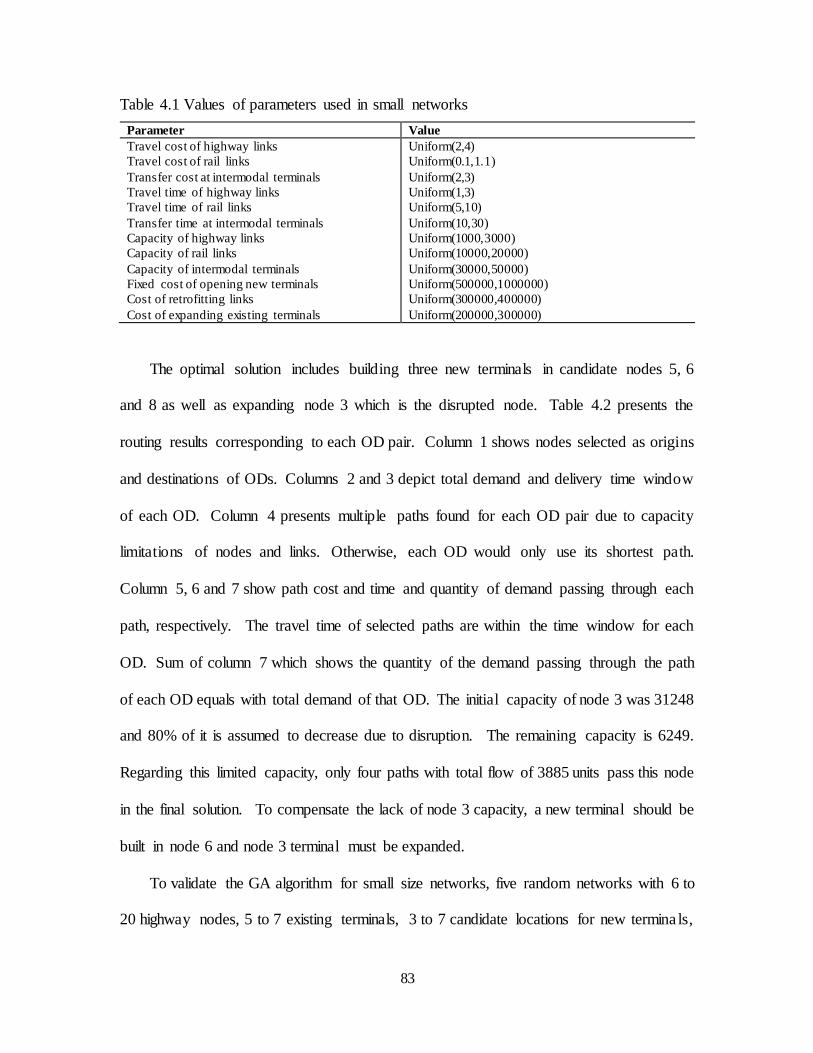
83

Table 4.1 Values of parameters used in small networks

Parameter Value

Travel cost of highway links

Travel cost of rail links

Transfer cost at intermodal terminals

Travel time of highway links

Travel time of rail links

Transfer time at intermodal terminals

Capacity of highway links

Capacity of rail links

Capacity of intermodal terminals

Fixed cost of opening new terminals

Cost of retrofitting links

Cost of expanding existing terminals

Uniform(2,4)

Uniform(0.1,1.1)

Uniform(2,3)

Uniform(1,3)

Uniform(5,10)

Uniform(10,30)

Uniform(1000,3000)

Uniform(10000,20000)

Uniform(30000,50000)

Uniform(500000,1000000)

Uniform(300000,400000)

Uniform(200000,300000)

The optimal solution includes building three new terminals in candidate nodes 5, 6

and 8 as well as expanding node 3 which is the disrupted node. Table 4.2 presents the

routing results corresponding to each OD pair. Column 1 shows nodes selected as origins

and destinations of ODs. Columns 2 and 3 depict total demand and delivery time window

of each OD. Column 4 presents multiple paths found for each OD pair due to capacity

limitations of nodes and links. Otherwise, each OD would only use its shortest path.

Column 5, 6 and 7 show path cost and time and quantity of demand passing through each

path, respectively. The travel time of selected paths are within the time window for each

OD. Sum of column 7 which shows the quantity of the demand passing through the path

of each OD equals with total demand of that OD. The initial capacity of node 3 was 31248

and 80% of it is assumed to decrease due to disruption. The remaining capacity is 6249.

Regarding this limited capacity, only four paths with total flow of 3885 units pass this node

in the final solution. To compensate the lack of node 3 capacity, a new terminal should be

built in node 6 and node 3 terminal must be expanded.

To validate the GA algorithm for small size networks, five random networks with 6 to

20 highway nodes, 5 to 7 existing terminals, 3 to 7 candidate locations for new termina ls,

84

30 to 100 links (including rail links), and 5 to 30 demand OD pairs were generated. Their

parameters were selected as mentioned in Table 4.1.

Table 4.2 Routing results of the small case study

OD Total

Demand

Delivery Time

Window (h)

Selected Paths Path

Cost

Path Travel

Time (h)

Flow on

Path

9-11 6395 122 9-10-11

9-1-2-11

9-10-2-11

9-5-2-11

9-14-13-11

9-14-6-13-11

9-5-6-3-12-11

Lost demand

6.11

9.59

7.42

11.1

10.41

11.71

17.14

5000

4.51

56.81

6.02

55.67

7.06

8.66

73.49

0

1380

1067

20

906

1158

629

1022

211

12-9 15777 131 12-11-10-9

12-3-6-1-9

12-3-6-5-9

12-8-2-5-9

Lost demand

9.32

13.21

13.93

15.02

5000

5.84

75.59

72.16

82.03

-

217

1067

275

1252

12966

11-14 8600 121 11-13-14

11-2-1-14

11-13-6-14

Lost demand

6.8

9.62

8.1

5000

4.74

57.27

6.34

-

2052

1992

900

3655

13-10 18272 123 13-11-10

13-6-1-2-10

13-3-6-1-2-10

Lost demand

6.68

13.28

15.7

5000

5.47

83.37

96.65

-

1165

724

1521

14862

14-12 1403 132 14-13-12

14-6-13-12

Lost demand

6.24

7.54

5000

4.29

5.89

-

894

509

0

Table 4.3 shows the validation results for these five small-sized networks. Column 1

shows the structure of the network. The five numbers in the parenthesis denote the number

of highway nodes, number of candidate terminals, number of existing terminals, number

of links, and number of OD pairs. Columns 2 and 3 indicate the computational time of the

GA and EE, respectively. Column 4 shows the gap between the GA objective function

value and the EE objective function value. As shown, the proposed GA algorithm was able

to find the same optimal solution as the EE algorithm, but in a much shorter time. The

largest problem among these small-sized networks took the EE algorithm almost four days

85

to obtain the solution while the GA algorithm was able to obtain the same solution within

a few minutes. These results demonstrate the efficiency and accuracy of the proposed GA

for solving the DINEP.

Table 4.3 Comparison of proposed hybrid GA algorithm versus EE algorithm for

solving DINEP

Problem Size GA time (sec) EE time (sec) Gap (%)* (6-3-5-30-5) 20 1,100 0.00 (10-5-5-50-10) 45 1,287 0.00 (20-5-7-100-20) 135 16,650 0.00 (20-5-7-100-25) 170 151,350 0.00 (20-7-7-100-30) 258 232,808 0.00

EEEEGA ObjObjObj )(*100*Gap

4.5.2 LARGER REALISTIC-SIZE NETWORKS

To demonstrate the potential real-world application of the proposed model and algorithm,

a test case is created using a realistic-sized intermodal and highway network and actual

freight demands. As mentioned, RINEP and DINEP are both NP-hard problems and

although EE is able to find the exact solution, a small increase in the network size will

exponentially increase its computational time and/or lead to insufficient memory on a

typical desktop computer with 8 GB of RAM (Meng and Wang, 2011). For this test case,

the EE algorithm was unable to obtain a solution, and thus, only the GA results are reported.

The test case involves an intermodal network of a Class 1 railroad which operates in

the Midwest and on the western side of the U.S. It is assumed that this company wishes to

gain a competitive advantage by improving and expanding its network. Additionally, to

make its business more attractive to shippers, this company wishes to strengthen its

network to withstand demand variations and network disruptions. The options to

86

strengthen the network include opening new intermodal terminals, expanding existing

terminals, and/or retrofitting existing rail links.

This company currently has 20 terminals in its intermodal network and it is

considering establishing new terminals at 10 potential locations. These candidate locations

are chosen because they are located near areas with higher disaster risks or freight demands.

As such, terminals at these locations could serve as backup terminals to deal with demand

influx and disruptions. The network includes 45 major cities which are connected via U.S.

interstates. Figures 4.4(a) and 4.4(b) show the intermodal rail network and the highway

network used for the test case, respectively.

For the purpose of this test case, highway distances and travel times were obtained

using Google Maps. Rail miles between intermodal terminals were obtained from the

railroad company’s website. It is assumed that the trains move at an average speed of 35

miles per hour. Terminals are assumed to operate 24/7 (24 hours per day, 7 days per week)

and that shipments incur a 24-hour dwell time at the terminal. The dwell time is 30 hours

for terminals that are opened 24/5. The various costs involved in intermodal transport were

taken from the ITIC Manual (2005). These include $0.7 transport cost per mile for rail

movements and $3.64 per mile for truck. A $150 transfer cost per container at an

intermodal terminal is used based on a South Carolina freight study.

The test case used a set of freight demand scenarios from the Freight Analysis

Framework (FAF3) (Battelle, 2011). Five demand scenarios were considered based on the

FAF3 freight forecast demands for the years 2020, 2025, 2030, 2035 and 2040. The test

case considers only those shipments that are likely to use intermodal transport, which are

those with an annual tonnage of more than 125 tons and a distance of more than 750 miles

87

(ITIC manual, 2005). Assuming an average of 80,000 lbs. weight limit for a 40-foot

container, FAF3 data were converted to their equivalent container units.

The test case considered eight disruption scenarios: (1) Burlington Rail Bridge

collapse (in Iowa), (2) hurricane in Southeast, (3) tornado in Midwest, (4) earthquake in

Northwest (Washington and Oregon), (5) ice storm in North and Midwest, (6) labor strike

at Los Angeles and Chicago terminals, (7) disaster in Texas, and (8) rail maintenance in

Texas and Arizona. For the scenarios with disrupted links, links which are directly

connected to the disrupted links had their capacities reduced but their reductions were

smaller than the disrupted links themselves. A total of 22 experiments involving different

disruption and demand scenarios were considered. We first solved the discrete problem

(DINEP) for the 22 experiments separately and then investigated the impact of integrat ing

all experiments for the final decision using the robust problem (RINEP).

4.5.2.1 EXPERIMENTAL RESULTS FOR DISCRETE PROBLEM

To investigate the impact of expansion on cost savings, each experiment’s optimal

cost with expansion is compared against the total transportation cost of the experiment with

no expansion (case 1) and expansion for only nominal-scenario (case 2); the nomina l

scenario is the scenario most likely to occur.

The results are shown in Table 4.4. Column 1 in Table 4.4 shows the experiment

number. Column 2 provides the demand and disruption scenarios considered for the

experiment.

88

(a)

(b)

Figure 4.4 Test case network: (a) Intermodal rail network; (b) Highway network

89

Column 3 provides the difference between the total transportation cost of No-

expansion (case 1) for the experiment and the optimal cost of the experiment with

expansion, column 4 provides the difference between the total transportation cost of the

Nominal-scenario expansion (case 2) for the experiment and the optimal cost of the

experiment with expansion, and column 5 presents the computational time of GA. The

nominal scenario (Experiment #0 in Table 4.4) is one that considers the demand for 2040,

but does not account for network disruption.

The results shown in Table 4.4 indicate that the railroad company will pay an extra

$250 million (average value of column 3) on average annually if it does not strengthen its

network to accommodate the growth in freight demand and future disruptions. This result

suggests that doing nothing will end up costing the company a significant amount of

money. By making some investments to strengthen the network to accommodate the

nominal scenario, the cost difference decreases to $113 million (average value of column

4). These results indicate that it is better (less costly over the long run) for the railroad

company to make the extra investments to strengthen the infrastructure than not to. Note

that some experiments do not incur extra cost compared to the nominal scenario because

their optimal expansion design is identical to that of the nominal experiment.

The optimal design of each scenario includes at most two new termina ls. Brookings

is selected in 90% (20 out of 22), Fort Smith in 18% (4 out of 22) and St. George in 10%

(2 out of 22) of experiments. Since around 80% of demand originates or ends in California,

a new terminal in Brookings as a backup for Los Angeles and Oakland will significantly

reduce the burden of congestion in these two terminals to deal with fluctuations in demand

and possible disruptions. Optimal links to retrofit and terminals to expand are more

90

affected by disruption that are different for each scenario rather than demand fluctuations.

The results of each disruption scenario are discussed in detail to justify this conclusion.

Experiment 1 considers scenario 1 with Burlington rail bridge collapse which makes

the Omaha-Chicago rail link out of service. The optimal solution allocates budget to build

a new terminal in Brookings and to retrofit Omaha-Chicago rail link. Brookings termina l

will accommodate the growth in future demand and retrofitting of the disrupted link

(replacing the bridge with a new one) will avoid the further collapse.

Considering experiment 2 with scenario 2 involving a hurricane in Louisiana and

Florida (it specifically impacts New Orleans terminal and links in Louisiana and Florida),

the optimal design concludes the establishment of two new terminals in Brookings and Fort

Smith. The new terminal in Fort Smith provides extra capacity to an alternate route for the

“Houston-New Orleans-Birmingham” route which is impacted by Hurricane and can be a

backup terminal for New Orleans.

Scenario 3 includes tornado occurring in Oklahoma, Arkansas, Nebraska, Missouri,

and Kansas states. It affects terminals in Omaha, Kansas City and St. Louis as well as

multiple rail and highway links in those states. The optimal design opens a new termina l

in Brookings, expands the terminal in Billings and retrofits six disrupted links. Expanding

a terminal in Billings will provide more capacity for an alternate route. Retrofitting six

disrupted links will mitigate the capacity reduction of these links in case of tornado.

The impact of expansion on network configuration can be understood by considering

experiment 4 with demand values for 2040 and disruption scenario 4 (Earthquake in North

part of Oregon and west side of Washington). In this scenario, the earthquake severely

degrades the capacity of Portland and Seattle terminals, as well as their connecting rail

91

links. It also reduces the capacity of highway links in those areas. The optimal solution

indicates that the expansion should include building a new terminal in Brookings, OR and

retrofitting the Portland-Seattle rail link. This is deemed reasonable as the Brookings

terminal can be considered as a backup terminal for the Portland terminal and retrofitt ing

Portland-Seattle link will ensure sufficient capacity to facilitate freight shipments to the

Brookings terminal.

Experiment 5 is impacted by disruption scenario 5 which is an ice storm in Midwest

of US. It impacts multiple states, including Utah, South Dakota, Wyoming, Montana,

Nebraska and Colorado, with similar severities. The optimal solution stablishes a new

terminal in Brookings, expands existing terminals in Seattle, Los Angeles, Oakland, St

Louis and St Paul and retrofits Billings-Spokane rail link. The Brookings terminal is a

backup to accommodate the increase of future demand in more demanding areas of the

network. Expanding terminals in Seattle, Los Angeles, Oakland and St Paul as well as

retrofitting Billings-Spokane rail link provides more capacity for the alternate route to

move east-west freight from the northern part of US rather than the disrupted Midwest part.

Expansion of St Louis also provides more capacity for the alternate route passing through

South of US.

The optimal design for experiment 6 with strike in Chicago and Los Angeles termina ls

suggests to open a new terminal in Brookings and expands the Los Angeles, Chicago,

Oakland and Kansas City terminals. This provides extra capacity in these terminals in case

of strike.

92

Experiment 7 deals with scenario 7 which considers a terrorist attack in Texas. It

affects terminals in Dallas and Houston and three rail links of that state. The optimal design

expands the terminal in Houston and retrofits the three disrupted links in that area.

The last experiment (scenario 8) considers the maintenance of Amarillo-Phoenix and Los

Angeles-Phoenix rails. The maintenance impacts congestion and capacity reduction in

multiple rail links in Texas. Although this scenario is not a natural or human-made

disruption, it deals with capacity reduction in a part of network due to inappropriate

planning for preventive maintenance. The optimal design suggests that despite building a

terminal in Brookings, the five disrupted rail links should be retrofitted to avoid long delays

in an important route through the west side of US.

Table 4.4 Experimental results for single scenarios

Experiment

#

Scenario

(demand year –

disruption

scenario)

Cost difference between no

expansion scenario and

experiment dependent

expansion

($)

Cost difference between

nominal scenario expansion

and experiment dependent

expansion

($)

0 2040-No disruption 158,104,588 0

1 2040-1 194,538,858 56,350,037

2 2040-2 164,814,523 0

3 2040-3 434,214,619 235,102,514

4 2040-4 137,980,502 49,480,200

5 2040-5 329,777,079 152,963,709

6 2040-6 373,592,268 292,797,864

7 2040-7 188,425,909 53,189,468

8 2020-No disruption 123,276,865 0

9 2020-1 203,866,442 63,880,608

10 2020-2 130,568,534 0

11 2020-3 344,788,771 179,283,058

12 2020-4 91,130,686 32,430,269

13 2020-5 284,051,633 129,664,657

14 2020-6 329,979,654 285,053,957

15 2020-7 151,825,758 27,523,964

16 2025-4 108,040,635 43,145,123

17 2030-6 148,169,117 0

18 2030-3 372,588,044 183,072,192

19 2035-2 152,989,073 0

20 2035-7 390,940,396 315,499,366

21 2040-8 652,125,611 395,066,849

93

In this work, it is assumed that expanded intermodal terminals can withstand disruptions.

However, in reality, there may be situations that are impossible to plan for, such as a labor

strike that shut down the entire terminal. From a modeling perspective, these situations

can be accounted for by relaxing the resiliency assumption of expanded terminals for

specific scenarios and replacing constraint 4.4 with the following constraint for both

optimization models.

SsNjvvvfjj ljljj

s

j

kw

w

jk

ws

k ,),)(1( 3,,

,

(4.16)

To better clarify this point, the experiment 6 that involves a labor strike at Los Angeles

and Chicago terminals can be considered. As mentioned before, the optimal design with

the initial assumption (expanded terminals are able to withstand disruptions) resulted in

expansion of Los Angeles, Chicago, Oakland and Kansas City terminals. This result is

reasonable because by expanding the terminals in Los Angeles and Chicago they will be

able to withstand the impact of disruptions. When the resiliency assumption for expanded

terminals is relaxed (i.e. replacing constraint 4.4 with constraint 4.16), it is surmised that

there is no benefit in expanding the terminals at Los Angeles and Chicago. Indeed, the

optimal design resulted in opening a new terminal in Las Vegas which is in close proximity

to Los Angeles and thus can serve as a backup terminal for the Los Angeles terminal. The

results indicated that opening a new terminal close to Los Angeles generates more profit

than opening a new terminal near Chicago. This is because for the test case more than 80%

of the freight shipments have origins or destinations in California.

To understand the need to include both types of risks (demand uncertainty and network

disruptions) in the robust decision, consider experiments 3, 11 and 18 with identica l

disruption scenario “3” but different demand scenarios. The optimal solution indicates that

94

a terminal should be opened at Brookings, OR for all three experiments. However, the

expanded terminals differ for each of these three experiments. “Billings”, “Houston”,

“Denver and Billings” are selected for expansion for experiments 3, 11, and 18,

respectively. These results validate that the optimal design for each disruption scenario is

demand-dependent. Similarly, consider experiments 0 to 8 that have identical demand

values but different disruption scenarios. The optimal solution for experiment 0 involves

opening two terminals, one at Brookings and one at Fort Smith. The optimal solution for

experiment 1 involves opening only one terminal at Brookings and retrofitting “Omaha -

Chicago”, “Omaha-Billings” and “Chicago-St. Paul” rail links. This is because the full

disruption of the rail bridge in Iowa disconnects the route from Omaha to Chicago and the

train should reroute to deliver the freight to Chicago. Hence, retrofitting Omaha-Chicago

link (which includes replacing the old bridge with a new one) will diminish the chance of

further disruptions remarkably. Retrofitting “Omaha-Billings” and “Chicago-St. Paul” (By

increasing their capacity) can make them to be an alternate route once the “Omaha-

Chicago” connection is disrupted. These results indicate the need to include different

demand and disruption scenarios in the network design problem. In other words, the robust

solution which considers various demand and disruption scenarios is necessary.

4.5.2.2 EXPERIMENTAL RESULTS FOR ROBUST PROBLEM

Table 4.5 shows the average increase in annual cost savings if all experiments were

included in the investment decision rather than only the nominal scenario by utilizing

RINEP. Column 1 in Table 4.5 shows the experiment number. Column 2 shows the

optimal objective function values of DINEP for each experiment. Columns 3 and 4 show

the regret values obtained from solving RINEP in term of cost and percentage for each

95

experiment, respectively. Regret shows the difference between the transportation cost of

the experiment under No-expansion, Nominal-expansion and robust expansion and the

transportation cost of the experiment with its own optimal expansion design. The results

show that the railroad company will incur an average of $73 million (average value of

column 3) extra in cost annually for each experiment under the robust design. This average

cost difference is almost 35% less on average (compared to average value of column 4 in

Table 4.4) compared to the case that considered only the nominal-scenario for expansion

decision.

Figure 4.5 depicts regret percentages of each experiment under the cases of No-

expansion, expansion considering only the nominal scenario and robust problem includ ing

all experiments. It can be seen in Figure 4.5 that out of the 22 experiments, the regret of

the robust expansion case is lower than the regret of the No-expansion case for all

experiments and lower than the regret of the Nominal-expansion case for 7 experiments.

It should be noted that although the regret for Nominal-expansion case is lower compared

to the robust expansion case for 70% of experiments, its regret is significantly higher for

the remaining 30% of the experiments (e.g. experiments 6, 14, and 20). The benefit of the

robust expansion case lies in the fact that it accounts for the worst case scenarios. The

average regret/cost ratio of 0.65% for the robust expansion case versus 0.96% for the

96

Nominal-expansion case confirms the overall advantage of the robust expansion case.

Figure 4.5 Regret for each experiment

The optimal design of the robust problem establishes a new terminal in Brookings.

This is a reasonable decision since almost 80% of the freight starts or ends in California.

Two terminals in Kansas City and Denver are selected for expansion. Since mult ip le

scenarios are included in the robust problem, the robust solution will work for any scenario.

Thus, the expansion of terminals in Kansas City and Denver can compensate the capacity

reduction in case of Ice Storm and Tornado scenarios in Midwest. Moreover, those can

provide extra capacity for an alternate route passing through Midwest if any scenario

happens in North and South of US (southern states are in danger of hurricane and

earthquakes are more likely in northwest and west states). The robust problem is more

sensitive to worst case scenario. Hence, the final results are more impacted by the worst

case scenario which in this case study is experiment 21 with scenario 8 (disruptions

happening in Texas and Arizona). The final links chosen for retrofitting verifies this

statement. Out of six rail links chosen to be retrofitted in the optimal solution, five of them

97

pass through Texas. Those are Houston-New Orleans, Houston-Amarillo, Dallas-

Houston, Phoenix-Amarillo and Dallas-Amarillo. The planner will benefit from this

decision in two folds. First, it improves the resiliency of the southern route in case of any

disruptions in Southern states, specifically if the worst case scenario happens (scenario 8).

Second, this makes the southern route a reliable alternative if any disaster happens in

Midwest and Northern states. Chicago-St. Paul is the sixth link in the optimal design to

retrofit as 30% of orders start or end in Chicago. This also improves the resiliency of the

route ending or staring from Chicago.

Table 4.5 Robust problem results

Experiment # *

sO ($) Regret ($) Regret (% )

0 16,542,321,527 11,163,213 0.07

1 16,553,001,838 85,842,258 0.52

2 16,550,281,391 29,196,426 0.18

3 16,554,666,496 164,646,494 0.99

4 16,569,423,659 78,826,799 0.48

5 16,557,288,485 176,262,511 1.06

6 16,553,050,966 96,787,324 0.58

7 16,553,016,517 59,947,876 0.36

8 7,620,998,025 14,006,736 0.18

9 7,630,861,372 81,625,026 1.07

10 7,634,230,809 17,966,755 0.24

11 7,668,495,535 117,622,713 1.53

12 7,659,882,813 44,990,212 0.59

13 7,635,051,519 145,639,333 1.91

14 7,634,721,012 85,889,871 1.12

15 7,634,536,576 50,736,989 0.66

16 9,557,474,545 58,282,051 0.61

17 11,616,846,502 22,059,076 0.19

18 11,655,954,662 129,678,603 1.11

19 13,608,715,581 17,730,949 0.13

20 13,609,371,300 113,291,957 0.83

21 16,553,325,372 2,105,791 0.01

To better understand how the network is affected by a single type of disaster instead

of a combination of disasters, additional analyses were performed where earthquakes and

tornadoes are analyzed separately. Figure 4.6 shows the U.S. earthquake risk map. As

98

shown, California, Washington, and a few of the Midwest states (Tennessee, Missouri,

Arkansas and Kentucky) have high risks of earthquakes. Five disruption scenarios with

different severities in these three areas are considered to assess the impact to the network

due to earthquakes only. Specifically, two scenarios consider earthquakes in California

with different severities (moderate and extensive damages), two consider earthquakes in

the Midwest (moderate and extensive damages), and one consider extreme earthquakes in

Washington and northern part of Oregon. Considering five demand scenarios for each

earthquake scenario, the robust problem has a total of 25 experiments. The robust solution

for this set of experiments indicate that a new terminal should be established in St. George,

Utah and to retrofit three rail links: Memphis-Birmingham, St. Louis-Kansas City, and

Memphis-Fort Smith. The result for the location to establish a new terminal is intuitive in

that St. George is closest to California (big market) but it is not in a high risk zone.

Therefore, this location would be ideal as a backup terminal for the California market;

should there be a disruption to terminals in California, this terminal can be used to send or

receive shipments from the rest of the U.S. Although terminals in Phoenix and St. Louis

are likely to be damaged severely in the event of an earthquake, they are located in smaller

markets, and thus, it is more cost-effective to retrofit potentially disrupted rail links in those

areas than to establish backup terminals.

Figure 4.7 shows the U.S. tornado risk map. As shown, the Midwest and Southern

states are more vulnerable to tornadoes. The tornado region stretches from North Texas to

Canada, with the core centers around Oklahoma, Kansas and Northern Texas, as well as

Alabama, Mississippi and Tennessee. Three tornado scenarios with different severities are

considered. The first scenario considers tornado in the East Tornado Alley, includ ing

99

Illinois, Kentucky, Tennessee, Alabama and Mississippi. The second scenario expands the

previous scenario by including Oklahoma, Arkansas, Nebraska, Missouri and Kansas. The

third scenario considers tornadoes in Oklahoma, Arkansas, Nebraska, Missouri, and

Kansas.

Figure 4.6 Earthquake risk map of US (http://geology.usgs.gov/)

Considering five demand scenarios for each tornado scenario, there is a total of 15

experiments in the robust problem. The robust solution for this set of experiments indicate

that a new terminal should be established in Brookings and to retrofit six rail links:

Memphis-Birmingham, Memphis-St. Louis, Atlanta-Birmingham, Amarillo-Kansas City,

Kansas City-Chicago, and Denver-Omaha. In contrast to the results from the earthquake

experiments, among the terminals close to California, Brookings is more desirable because

it is furthest away from the tornado region. Similar to the earthquake results, it is more

cost-effective to retrofit the aforementioned selected links than to establish backup

terminals in the tornado region.

100

Figure 4.7 Tornado risk map in US (http://strangesounds.org/)

Based on the results on the case study, it can be concluded that rail operators should

consider the following guidelines: (1) new terminals should be established close to a large

market area which is less likely to be disrupted and be located as far away from the exact

location of potential disruption in that area (e.g. position the terminal as far as inland as

possible if the market area has the potential to incur a storm surge); (2) within a disrupted

area, it is more beneficial to retrofit a high-risk link than to expand an existing terminal (it

is counterproductive to expand a terminal that is not accessible by rail whereas a retrofitted

link will enable trains to get to an alternate terminal); (3) among the existing termina ls,

those located close to higher risk areas should be expanded (these expanded terminals can

101

serve as alternate terminals for cargo that are planned to originate or terminate at the

disrupted terminals.

It should be noted that our policy recommendations are drawn from the set of scenarios

that we examined, and thus, they may or may not reflect the actual operating conditions

faced by the railroad operator. However, the developed model can be used to examine

other types of scenarios. Moreover, the developed model can be used to perform

sensitivity analyses to gain insights into different expansion strategies (e.g. what is the

benefit of adding one versus two new terminals to the network).

4.6 CONCLUSIONS

This paper developed a robust and reliable mixed-integer linear model for expanding an

intermodal freight network which can cope with fluctuations in demands and disruptions

with infrastructure. The model employs a min-max regret approach to identify a network

design that is best suited to safe guard against the worst case scenario. A hybrid genetic

algorithm which uses column generation to determine the freight flows was developed to

solve the proposed model. The proposed algorithm was found to perform well in terms of

solution quality and computational time compared against an exhaustive enumerat ion

algorithm for a set of small-sized networks and a larger realistic-size intermodal/highway

network in US. The results indicated that it is better (less costly over the long run) to make

the extra investments to strengthen the infrastructure than not to. It also indicated that

when deciding on the infrastructure strengthening options, it is best to include as many

demand and supply scenarios as possible.

This work can be extended by including other modes of transportation and by

considering scheduled time tables at intermodal terminals. An additional challenge that

102

could be considered includes utilizing queuing models to account for capacity constraint at

intermodal terminals. Lastly, this work can be improved by developing exact algorithms

to solve the model.

Long term, this model and its subsequent enhancements could be used by railroad

operators as well as transportation planners to identify weak links in the intermodal freight

network and to evaluate the capacity of the existing infrastructure. This is particular ly

important for disaster planning in terms of quantifying the resiliency of the network and

improving the network’s resiliency and reliability under extreme events. Another aspect of

the model that can be improved is to consider explicitly the temporal dimension; that is,

consider how the network is affected by the incremental supply and demand changes over

time.

103

CHAPTER 5: A RELIABLE MULTI-PERIOD INTERMODAL FREIGHT NETWORK EXPANSION PROBLEM3

3 Fotuhi, F., and Huynh, N., Submitted to Journal of Computers and Industrial Engineering, 3-14-2017

104

ABSTRACT

This paper addresses the intermodal freight network expansion problem consisting of

multiple periods. In each period, the objective is to determine the locations of new

intermodal terminals, the amount of capacity to add to existing terminals, and the existing

rail links to retrofit. The multi-period planning problem has the added complexity of

determining which period a particular improvement should be made given a limited budget

for each time period. A probabilistic robust mathematical model is proposed to address

these decisions and uncertainties in the network. Due to the complexity of this model, a

hybrid Simulated Annealing (SA) algorithm is proposed to solve the problem and its

applicability is demonstrated via two numerical examples. Important managerial insights

are drawn and discussed on the benefits of utilizing the multi-period approach.

5.1 INTRODUCTION

An efficient freight transportation system is crucial to the competitiveness of the U.S. in

global trade (Ortiz et al., 2007). In the last few decades, tax regulations, green policies

(Macharis et al., 2011) and alternative options to move freight at a lower cost have

promoted the use of intermodal transportation. Intermodal transportation is defined as

movement of goods in the same load units with more than one mode of transport without

handling goods themselves while transferring between modes at intermodal terminals (Lin

et al., 2014). Around 40% of the total freight volume in U.S. are intermodal shipments.

This volume is forecasted to increase 3.25 times by 2040 (Bureau of Transportation

Statistics, 2012). To cope with the increasing freight demands and aging infrastructure,

intermodal service providers need to continually plan for upgrades of their existing

networks, as well as plan for expansion to grow their market share. These expansion plans

105

are long term and are subject to various uncertainties such as changing demands and

infrastructure changes. Additionally, the supply capacity of the network may be impacted

by natural or man-made disruptions, such as the U.S. West Coast labor dispute in 2002 and

damages to oil storage tanks in states of Texas and Louisiana due to hurricane Katrina in

2005 (D’ Amico, 2002; Sarkar et al., 2002; Godoy, 2007). Moreover, there are potential

new markets which may not have been considered in freight prediction models such as the

Freight Analysis Framework (Fotuhi and Huynh, 2015). These factors necessitate the

consideration of demand and supply uncertainties in network expansion plans.

One of the principal features of intermodal network design and expansion models is

their multi-period nature due to their variable parameters over time (cost, demand, and

resources) (Contreras et al., 2011). Additionally, expansion projects require extensive

capital investment which may not be available to the stakeholder at the beginning of the

planning horizon. These facts are often ignored in the traditional single-period network

design problems (Melo et al., 2006). In the multi-period expansion problem, the planning

horizon is divided into multiple time periods and the network is incrementally expanded

over the planning period, much like how Class 1 railroad companies expand their network

over time. Recent examples include CSX building new terminals in Montreal, Pittsburg,

and Central Florida. The multi-period approach provides the stakeholder benefits. First, it

mitigates the financial burden on the company to acquire significant capital in a short

period of time to expand the network. Second, it improves resource management by

building terminals “just-in-time,” that is, terminals are built only when they are needed.

Third and lastly, a more accurate route planning can be done for different time periods

utilizing the available resources at that period.

106

Nagy and Salhi (2007) introduced the concept of multi-period location-routing

problems considering different time scales for location and routing decisions. They

indicated that a multi-period location-routing framework with shorter routing periods

within location decision periods is a better approach to modeling real world location-

routing decisions. Their motivation for adopting the multi-period decision problem is the

frequent changes in cost and demand over time which significantly impact routing

decisions. The same case can be made for intermodal freight network expansion problem.

A few studies have addressed the intermodal network expansion problem (Meng and

Wang, 2011; Fotuhi and Huynh, 2016); However, to date, there has been only one study

that used the multi-period approach for the intermodal network expansion problem

(Benedyk et al, 2016). In their study, a new model was proposed to evaluate different

expansion scenarios over multiple time periods. Their model finds the optimal location for

new terminals, determines the optimal capacities for existing terminals and determines the

allocation of origin-destination (OD) demand pairs to terminals. Note that in their model,

expansion and allocation decisions are made within the same period regardless of possible

disruptions that might happen in the network

The specific objective of this paper is to develop a model for Reliable Multi-Period

Intermodal Network Expansion Problem (RMPINEP). An inherent challenge with

developing such a model is that expansion and routing decisions are made at different time

periods. To model this, it is assumed that the planning horizon is divided into a set of short

time periods for routing decisions. However, expansion decisions are made at a subset of

these periods and they remain unchanged throughout the planning horizon. It is also

assumed that disruptions only happen at expansion time periods and the network recovers

107

from them through the subsequent routing periods until the next expansion period. A robust

optimization approach is used to account for forecasted demand errors and possible

disruptions during the planning horizon. The contributions of this paper are: (1)

development of a new model for multi-period intermodal freight network expansion

problem, (2) the developed model considers different time periods for expansion and

routing decisions, (3) the developed model incorporates different sources of uncertainty,

and (4) development of a meta-heuristic to solve the developed model for large-sized

instances.

5.2 LITERATURE REVIEW

Recently, SteadieSeifi et al. (2014) provided a comprehensive review of previous studies

in multimodal freight transportation planning classified into strategic, tactical and

operational planning levels. Strategic decisions deal with investment in infrastruc ture

which may involve adding and/or maintaining intermodal terminals and network links. The

intermodal terminal location problem was first studied by Arnold, Peeters, Thomas and

Marchand (2001). They proposed a model to find optimal locations of uncapacitated

intermodal terminals in a rail-road intermodal network with unimodal (direct) and

intermodal shipping options. In a follow-up work, they improved their previous model by

considering intermodal terminals as network arcs to reduce number of decision variables

in their model (Arnold et al., 2004). Ishfaq and Sox (2011) formulated a model for finding

the optimal locations of intermodal terminals and allocation of commodities with limited

time windows to pairs of terminals. Their model ignored the direct shipping option

between origins and destinations. Sörensen et al. (2012) added limited capacity at

intermodal terminals and direct shipping option to the Ishfaq and Sox (2011) model, but

108

ignored the time window constraints for shipments. Their model was modified by Lin et

al. (2014) to reduce redundant variables.

The aforementioned articles assumed there is no uncertainty involved in problem

parameters. However, terminal locations are long-term decisions with many uncertaint ies

arising from changes in demand, cost, capacity, and network disruptions. Uncertainty in

demand have been widely investigated in network design problems in the last decade.

Atamturk and Zhang (2007) proposed a robust two-stage network design model with

uncertain demands. The binary link design variables were defined in the first stage and

flow was assigned to the network after the actual values of the demand were revealed in

the second stage. Yang (2009) formulated a stochastic two-stage air freight hub network

design problem. He assumed that the demand is uncertain and varies seasonally. Its model

found the optimal number and location of hubs in the first stage and subsequently

determined the freight routes in the second stage. Contreras et al. (2011) proposed a model

for stochastic uncapacitated hub location problem with uncertain demand and

transportation costs. Shahabi and Unnikrishnan (2014) considered uncertain demand

within a hub network design problem and showed that more hubs should be opened

compared to the deterministic hub network design decisions. Fotuhi and Huynh (2015)

were the first to consider uncertain demand for competitive intermodal terminal location

problem. They proposed a robust model to find the optimal number, location and size of

intermodal terminals and allocation of freight flow to the network for a private rail road

company. They showed that terminals that have larger capacities are better equipped in

dealing with demand variations.

109

Capacity is another source of uncertainty which may be caused by natural or human-

made disasters in network elements (links or nodes). These disruptions can lead to delay

in order delivery, loss of market share, and higher transportation costs. For this reason, it

is recommended that capacity be included in models to incorporate reliability in network

design decisions (Peng et al., 2011). D'Este and Taylor (2003) suggested that it is best to

invest on the weakest elements in the network to reduce network vulnerability to

disruptions. Several studies have incorporated disruptions in transportation network design

decisions. Rios et al. (2000) formulated a capacitated network design problem with

disruptions to network links. Their model determined which set of links to open and their

corresponding capacities to guarantee network survival in case of disruptions. Viswanath

and Peeta (2003) proposed a multi-commodity maximal covering network design model to

address network risks due to earthquakes. Their model identified critical routes in the

network and higher risk bridges within those routes that need to be retrofitted. Desai and

Sen (2010) considered link failure risk in a reliable network design model which allocated

resources to mitigate the disruption impacts on higher risk links in the network. Peeta et

al. (2010) formulated an investment model to retrofit higher risk links in a highway

network. A few studies have incorporated facility (node) disruptions in logistics and

transportation network design problems. Peng et al. (2011) proposed a model for reliable

logistics network design problem with disruption risk at suppliers and distribution centers.

Their model found optimal locations for these facilities and flow allocation to the

corresponding network minimizing disruption risks. An et al. (2011) considered

disruptions in transshipment nodes for a hub-and-spoke network design problem. Their

model found the optimal locations of backup hubs while minimizing the expected

110

transportation cost for normal and disrupted situations. Marufuzzaman et al. (2014)

incorporated disruptions at intermodal terminals in a biofuel supply chain design problem.

Their model found locations of intermodal terminals and bio-refineries while minimizing

total fixed and transportation costs. Miller-Hooks et al. (2012) considered disruptions in

both network links and terminals of an intermodal network design problem. They found

best recovery and pre-disaster policies to maximize network resiliency against disruptions.

Fotuhi and Huynh (2016) proposed a model for intermodal network expansion problem

considering link and terminal failures. They also included uncertain demand in their

expansion and routing decisions as well. Their model found optimal locations of new

intermodal terminals, existing terminals to expand and less resilient links of the network to

retrofit to increase network resiliency to disruptions.

One of the main characteristics of network design models which have been neglected

in the aforementioned studies is their dynamic nature (i.e., multi-period planning). The

literature on multi-period transportation network design is scarce. Contreras et al. (2011)

were the first to model a multi-period hub location problem. Their model identified when

and where to open new hubs and to close open hubs as well as flow assignment to pairs of

open hubs. They assumed that the flow fluctuates over time. Taghipourian et al. (2012)

employed the concept of multi-period planning for a virtual hub network design problem

of airline industries. They also assumed that hubs are uncapcitated and hubs opened in one

period might be closed in later periods. Recently, Gelareh et al. (2015) developed an

uncapacitated multi-period hub location model for a liner shipping provider. They assumed

that the service provider will lease one hub in a period and will end the lease in another

period. The objective of their model is to determine when to lease a new hub and when to

111

end the lease for an operating hub. They considered a limited budget available to lease

new hubs and operation of existing hubs in the system for each period. Alumur et al. (2015)

formulated multi-period single and multiple-allocation hub location problems with limited

capacities at hubs. The objective of their model is to determine when and where to locate

a new hub and which open hubs to expand to minimize total construction, expansion and

routing costs. They assumed that once a hub is opened in a period it will remain open

throughout the entire planning horizon. In a recent work, Benedyk et al. (2016) proposed

a location-allocation model for intermodal network expansion problem over multiple time

periods with uncertain demands. They considered new intermodal terminals to add to the

network and expanding existing terminals. They demonstrated their model on a sample

freight network within the U.S. and evaluated a few expansion scenarios on a 10-year

planning horizon. Their model found optimal allocation of shippers and receivers to

transfer points (intermodal terminals and ports) but did not find specific routes for them.

This work extends the work of Fotuhi and Huynh (2016) and incorporates the mult i-

period planning approach proposed by Benedyk et al. (2016) for intermodal freight

networks. It also incorporates the idea from Albareda-Sambola et al. (2012) of considering

different routing and design time scales. To the best of the authors’ knowledge, this is the

first work in intermodal freight network expansion that considers multi-period planning

with different time scales for expansion and routing decisions and considering demand and

supply uncertainties.

5.3 PROBLEM STATEMENT

RMPINEP is a network expansion problem of an existing rail-road intermodal network

with a finite planning horizon, uncertain demand and disruption risk at network termina ls

112

and links. Commodities are delivered to the customers using intermodal option via a set of

intermodal terminals or directly with trucks. The network features 1N , sets of existing

terminals, 2N , sets of candidate nodes for installing new terminals, 1A , sets of highway

links, and 2A , sets of rail links. The planning horizon is divided into T time periods (years,

quarters of years). As mentioned before, two different time scales are considered for

routing and expansion decisions. While routing decisions are made at each time Tt , a IT

subset of time periods of the planning horizon, TTI , are selected for strategic expansion

decisions. At each period Tt , the demand for tW sets of Origin-Destination (OD) pairs

selected from 3N , sets of highway nodes (cities) is routed through the network. twK is the

set of paths for OD pair tWw at routing period Tt .

This work considers the following assumptions:

Terminals opened at each expansion period stay opened through the planning horizon.

Capacity of expanded terminals is not reduced through the planning horizon.

Transfer time and cost are only considered for terminals that the shipment changes

mode.

It is assumed that capacity modules with different sizes are available for each existing

terminal. At each expansion period, at most one capacity module can be selected from

a predefined set of capacity modules. tjL is the set of capacity modules for termina l

1Nj at expansion period ITt .

A penalty cost is considered for shipments violating delivery time windows.

OD pairs pattern and their corresponding flows change during the planning horizon.

There is a limited budget tB for expansion decisions at each expansion period ITt .

113

Expansion and routing decisions are affected by a set of disruption and demand

scenarios, tS for each expansion period ITt and its underlying routing periods. It is

assumed that disruption damages decrease through the routing sub-periods of an

expansion period.

The optimal decision seeks to find when and where to open new intermodal termina ls,

when to expand an existing intermodal terminal and its optimal capacity module, and

retrofitting priority of higher risk links in each expansion period as well as routing of fre ight

flow at each routing period minimizing total expansion costs and expected routing costs

over all scenarios.

5.3.1 ILLUSTRATIVE EXAMPLE

Figure 5.1 depicts a sample solution of RMPINEP. The network has 3 existing termina ls,

3 rail links, 3 candidate terminals, 4 cities, 2 OD pairs (1-3,2-4), 4 time periods and

}4,2{IT . Blue lines show the optimal routes for each OD pair. As illustrated in fig. 1,

one terminal is fully disrupted at t=2. Hence the demand for OD pair (1-3) is rerouted by

utilizing a new terminal which is opened at this period. Time 3 is a routing period and the

disrupted terminal is partially recovered. Accordingly, the demand for OD pair (1-3) is

partially met by the disrupted terminal. At t=4, the demand for OD pair (1-3) is increased

and one link in one of its optimal routes in the previous period is out of operation.

However, one terminal in the other route is expanded to fully meet the demand for this OD.

114

5.4 MATHEMATICAL MODEL

A robust path-based mixed integer model is proposed for RMPINEP. Model parameters

and notations are mentioned as follows:

Parameters

at : Average travel time on link )( 21 AAa

j : Average transfer time at terminal )( 21 NNj

tswT : Time window for OD pair tWw under scenario s at expansion period ITt

tjF: Annual fixed cost of opening candidate terminal 2Nj at expansion period ITt

tac : Travel cost per unit of flow on link )( 21 AAa at routing period Tt

1

t=1 t=2

t=3 t=4

: Candidate terminals; : Existing terminals; : Existing rail links; : Candidate rail links

: Cities (Origins/Destinations); : Expanded terminals; : Disruption at terminals; : Disruption at

links

2 3

4 1 4

2 3

1

2

4

3

1

2

4

3

Figure 5.1 A sample solution of the problem.

115

tjc : Transfer cost at terminal )( 21 NNj per unit of flow at routing period Tt

tjl

jC

: Capacity expansion cost for module tj

tj Ll

at terminal 1Nj

jv : Current capacity of existing terminal and capacity of new terminals )( 21 NNj

ae : Capacity of link )( 21 AAa

tsw

td : Demand of OD pair tWw under scenario tt Ss at routing period Tt

tsjt : Disruption percentage of terminal )( 21 NNj under scenario ts at routing period

Tt

tsa

t : Disruption percentage of link )( 21 AAa under scenario ts at routing period Tt

tah : Hardening cost of link 2Aa at expansion period ITt

ts : If expanded terminals withstand disruptions under scenario tt Ss

ts : If retrofitted rail links withstand disruptions under scenario tt Ss

tsp: Probability of occurrence of scenario tt Ss at expansion period ITt

tws

akt : path-arc incidence (= 1 if link )( 21 AAa is used in path k for OD pair tWw under

scenario tt Ss at routing period Tt ; 0 otherwise)

tws

jkt : path-terminal incidence (=1 if shipments change mode at terminal )( 21 NNj in

path k for OD pair tWw under scenario tt Ss at routing period Tt ; 0 otherwise)

RMPINEP encompasses strategic (expansion) and operational (routing) decision

variables. Once strategic decision variables are determined at each expansion period,

routing decision variables are found for subsequent routing periods. The decision variables

are as follows:

Decision Variables

116

tjy : 1, if a terminal is opened at node 2Nj at expansion period ITt ; 0, otherwise

t

lj tj

v

,

' : 1, if expansion design tjl is selected for terminal 1Nj at expansion period ITt ; 0,

otherwise

taz : 1, If link 2Aa is hardened at expansion period ITt ;0, otherwise

tws

ktx : 1, if a shipment for OD pair tWw uses path k under scenario tt Ss at routing period

Tt

tws

ktf : Amount of freight flow for OD pair tWw on path k under scenario tt Ss at routing

period Tt

Using the aforementioned variables and parameters, RMPINEP is formulated as

follows:

Ttswk

t

k

ws

kts

TtNj TtNj TtAa

t

a

t

alj

t

lj

t

j

t

j cfphzCvyFMin t

tjj

,,,, , ,

,,

2 1 2

' (5-1)

Subject to:

TtTtSsNjvvvf tt

tt

t

ljljj

ts

js

kw

ws

jkt

ws

kt jj

t

t

tt

,,,,])1[( 1,,

,

(5-2)

TtSsNjvvvf tt

tt

t

ljljj

ts

js

kw

ws

jkt

ws

kt jj

t

t

tt

,,),)(1)(1( 1,,

,

(5-3)

TtSsNjvf ttj

kw

ws

jkt

ws

ktt ,,, 2

,

(5-4)

Tt ,'

2 1 2

,,

t

Nj Nj Aa

ta

talj

tlj

tj

tj BhzCvyF

jj (5-5)

TtNjvj

jlj

l

t

,,1' 1, (5-6)

TtSsAaef tt

kw

a

ts

a

ws

akt

ws

ktttt ,,,)1( 1

,

(5-7)

117

TtSsAaezf tt

kw

a

tt

t

a

ts

as

ws

akt

ws

ktt

t

tt

,,,))1(1( 2

,

(5-8)

TtSsAaef tt

kw

a

ts

as

wt

ak

ws

ktt

t

t

,,,)1)(1( 2

,

(5-9)

TtSsKkWwxMT

tzt

tt

t

w

ws

kt

ts

w

Nj

wt

jkj

Nj

wt

jkj

ts

j

wt

aka

Aa tt

t

a

ts

a

wt

aka

Aa

ts

a

tt

ttt

,,,),1(

))(1())1(1()1(2121

(5-10)

TtSsWwKkMxf ttw

ws

kt

ws

kttt ,,,, (5-11)

tt

t

t

j

ws

jkt

kw

ws

kt SsNjyMx tt

,, 2

,

(5-12)

TtSsWwdf ttt

ts

wt

k

ws

kttt ,,, (5-13)

2,1 NjyTt

t

j

(5-14)

2,1 AazTt

t

a

(5-15)

ttt

ws

kt

ws

ktlj

t

a

t

j SsNjAaWwfxvzy tt

j

,,,,0},1,0{,,, 22

'

, (5-16)

Objective function (5-1) minimizes total expansion cost and expected routing cost over

all scenarios and routing periods. Constraints (5-2) and (5-3) ensure that capacity of

existing terminals are not violated for all routing periods. If expanded terminals stay

resilient under a specific scenario at later periods, constraints (5-2) are activated.

Otherwise, Constraints (5-3) are utilized. Constraints (5-4) guarantee that capacity of new

terminals are not violated for all routing periods. Constraints (5-5) limit expansion

decisions by the available budget at each expansion period. Constraints (5-6) ensure that

at most one capacity module can be selected for existing terminals. Constraints (5-7)

prohibits capacity violation of highway links. Constraints (5-8) and (5-9) guarantee that

capacity of rail links are not violated. Like the assumption for constraints (5-2) and (5-3),

118

constraints (5-8) are activated if hardened links stay resilient in case of disruptions and

constraints (5-9) are activated in the opposite case. Constraints (5-10) ensure that time

windows are not violated. Constraints (5-11) and (5-12) assure that freight flow are

assigned to open terminals. Constraints (5-13) guarantees that all demand is met for each

OD pair. Due to capacity limitations and time windows, such an assumption is not realistic.

Hence, unmet demand for each OD pair is considered as the amount of flow over a

hypothetical path between origin and destination of an OD pair with a penalty cost.

Constraints (5-14) ensure that a candidate node can be opened at most once over all

expansion periods. Similarly, constraints (5-15) guarantee that each rail link is retrofitted

at most once over the planning horizon. Constraints (5-16) are the integrality of decision

variables.

5.5 SOLUTION METHOD

RMPINEP reduces to the discrete network design problem when considering single period

with no uncertainty in parameters. Since the discrete network design problem is NP-hard

(Meng and Wang, 2011), RMPINEP is NP-hard as well. This problem is computationa lly

intractable due to the following reasons. First, ||*|*|*||)*1|(| 212 1ALNNT NjI possible

configurations of strategic decision variables should be examined for optimal decision.

Although budget constraint limits this number, a remarkable set of configurations stay

feasible for evaluation. On the other hand, there is a huge number of possible paths for

each OD pair. It is difficult and computationally expensive to enumerate all of them for

each configuration involving multiple scenarios and their corresponding routing periods.

Traditional optimization solvers are not able to solve this problem even for very small

networks due to the huge number of variables and constraint. Hence, a hybrid Simulated

119

Annealing (SA) algorithm integrated with Column Generation (CG) for routing decisions

is proposed to solve the problem. SA finds optimal values for strategic decision variables.

Once these variables are determined, CG is used to find freight flow assignment for each

routing period under each scenario.

SA was inspired by the annealing process in metals. The metal is heated to a high

temperature and is gradually cooled down to attain to its optimal shape. Molecules can

move freely in high temperatures but they are stuck in lower temperatures. SA, a

probabilistic search algorithm, starts with an initial solution at a high temperature and

explores the nearby solutions. If the neighbor solution is better, then it is accepted as the

current solution. Otherwise, the algorithm accepts a worse solution with a probability. As

it cools down, this probability becomes lower. The idea of accepting a non-improving

solution is to escape from local optima. A complete overview of the algorithm can be

found in Kirkpatrick et al. (1983).

5.5.1 SOLUTION REPRESENTATION

The feasible strategic solutions are coded as integer single dimensional arrays. Each array

consists of two sections for new terminal location and link retrofitting decisions and || IT

sections for capacity expansion of existing terminals. Figure 5.2 depicts a sample

representation of a solution considering a network with 3 existing terminals, 2 candidate

terminals, 4 links and 2 expansion periods. As shown, candidate terminal 1 never opens

through the planning horizon while candidate terminal 2 will be opened at period 1. Links

1 and 3 are not retrofitted while links 2 and 4 are retrofitted at periods 2 and 1, respectively.

In expansion period 1T , capacity module 1 is selected for existing terminal 1. Existing

terminals 2 and 3 are not expanded at this period. Capacity modules 1 and 2 are selected

120

for existing terminals 2 and 3 at time 2T , respectively. Existing terminal 1 is not expanded

at this period. Each configuration is checked to avoid budget violation. The algorithm

generates a random initial solution and checks its feasibility regarding budget constraint.

Once the strategic variables are fixed, RMPINEP reduces to the Capacitated Multi-

Commodity Intermodal Network Flow Problem with Time Windows (CMINFPT), one for

each routing period and scenario. The CG algorithm embedded with an intermodal label

setting algorithm proposed by Fotuhi and Huynh (2016) is used to assign freight flow to

the network. The objective function is computed once routing subproblems are solved.

5.5.2 NEIGHBORHOOD SEARCH MECHANISM

For each solution, a neighboring solution is generated as follows:

Step 1: Select a random strategic variable (candidate terminal, link or existing termina l),

xx and a random period, tt.

Step 2: If xx is a candidate terminal,

If the corresponding value of xx equals tt,

Fixed-cost/capacity ratio ( vF tt / ) is computed for candidate terminals which are

not opened at tt. Terminal with lowest ratio is opened at tt and xx is closed for

the whole planning horizon. If there is no terminal opened at other time periods,

xx is closed and no terminal is selected to open at tt.

Candidate

Terminals Links

0 1 0 2 0 1 1 0 0 0 1 2

Existing Terminals

Figure 5.2 A sample representation of a solution.

121

Else,

Fixed-cost/capacity ratio ( vF tt / ) is computed for candidate terminals opened at

tt. Terminal with highest ratio is closed for the whole planning horizon and xx

is opened at tt. If there is no new terminal at tt, xx will be opened at this time

period.

Else if xx is an existing terminal,

Two options are available for neighborhood search:

1. Randomly change the capacity module of xx at time tt to a different one from

its available modules.

2. Swap the capacity modules of xx and a random existing terminal, yy, at tt.

Modules can be exchanged if they are within the maximum number of

eligible modules of the alternate terminal at tt.

Else,

If the corresponding value of xx equals tt,

Harden-cost/capacity ratio ( ehtt / ) is computed for links which are not retrofitted

at tt. Link with lowest ratio is retrofitted at tt and xx is not maintained for the

whole planning horizon. If there is no link which is retrofitted at other time

periods, xx is not maintained and no link is selected for maintenance at tt.

Else,

Harden-cost/capacity ratio ( ehtt / ) is computed for retrofitted links at tt. Link

with highest ratio is not retrofitted for the whole planning horizon and xx is

retrofitted at tt. If there is no retrofitted link at tt, xx will be retrofitted at this

period.

122

Step 3: Check the budget constraint for the new configuration. If the configuration is not

feasible, discard it and go to step 1.

5.5.3 EVALUATE THE NEIGHBORING SOLUTION

Once a feasible neighboring solution is generated, freight flow is assigned to the network

for all routing periods and the objective function value (C(λ)) of this configuration is

computed. If C(λ) <= C(λ0), C(λ0) is the objective function of the current solution, the new

configuration is accepted as the current solution and C(λ0)=C(λ). Otherwise, the

probability of accepting this non-improving solution is determined by Boltzman function

/e . is the difference between C(λ0) and C(λ) and is the current temperature. A

random number ]1,0[ is generated. The inferior neighboring solution is accepted if

/ e . Otherwise the current solution stays the same. If C(λ) is smaller than C(λ*), the

best solution found so far, C(λ*)=C(λ).

5.5.4 COOLING SCHEDULE

A predefined number of solutions K, known as neighborhood size, are generated and

evaluated at each temperature. The temperature is decreased with the following function

after k neighboring solutions are evaluated.

ii *1

Where )1,0( is the cooling rate by which the temperature is decreased. The algorithm

terminates if 0 i , 0 is the frozen temperature. It may also terminate if the solution is

not improved for a predefined number of iterations.

5.6 COMPUTATIONAL EXPERIMENTS

The proposed solution algorithm is coded in MATLAB R2016 and all experiments are run

on a desktop computer with an Intel Core 2 Duo 2.66 GHz processor and 24 GB of RAM.

123

A random small network is used to validate the proposed model and algorithm in terms of

optimality and computational time. The application of the model on real-sized network is

also investigated.

5.6.1 SMALL SIZE NETWORK

A small hypothetical network with 10 cities, 3 existing terminals, 4 candidate terminals, 10

periods including 2 expansion periods and 10 routing periods (10 years) is considered.

Expansion decisions are made at periods 1 and 6 with 4 and 3 scenarios respectively. At

each routing period, 6 to 10 random OD pairs are selected from the cities. Figure 5.3

illustrates the network. It is assumed that with 85% chance, no disruption happens at the

first expansion period but there is a 5% chance of disruption at existing terminal 3 and all

links connected to it, 5% chance of disruption at existing terminal 1 and all its inbound and

outbound links and a 5% chance of disruptions at all outbound links from city 2. The

second expansion period faces 90% chance of no disruption, 5% chance of disruption at

terminal 2 and all links connected to it and 5% chance of disruption at outbound links from

cities 1 and 3. Table 5.1 presents the problem parameters considered for the small

hypothetical network.

This example is solved with both SA and Exhaustive Enumeration (EE). SA could find

the optimal solution in 1 hour while it took the EE more than one day to find the optimal

solution. The optimal solution involves opening candidate terminals 4 and 2 at the first

and second expansion periods, respectively. Figure 5.4 illustrates the impact of mult i-

period planning on routing decisions. Specifically, it shows the routing results of one of

OD pairs (1-10) under the second expansion period for the second scenario.

124

Table 5.1 parameters of small hypothetical network

Parameter Value

Travel cost on highway links

Travel cost on rail links

Transfer cost at intermodal terminals

Travel time on highway links

Travel time on rail links

Transfer time at intermodal terminals

Capacity of highway links

Capacity of rail links

Capacity of intermodal terminals

Fixed cost of opening new terminals

Cost of retrofitting links

Cost of expanding existing terminals

Uniform(2,4)

Uniform(0.1,1.1)

Uniform(2,3)

Uniform(1,3)

Uniform(5,10)

Uniform(10,30)

Uniform(1000,3000)

Uniform(10000,20000)

Uniform(30000,50000)

Uniform(500000,1000000)

Uniform(300000,400000)

Uniform(200000,300000)

Figure 5.3 Network of the small case study.

: Existing Terminal : Candidate Terminal : City

: Highway Links : Drayage Links : Rail Links

125

As shown in Figure 5.4, four different paths are selected for this OD pair through the

routing subperiods. Routing periods 1, 3 and 4 have the same set of routes while periods

2 and 5 have one route in common with the other three routing periods. The orange route

which is selected for all periods is the shortest path for this OD pair. However, due to

limited capacity, the flow is partially covered by this route and the rest is moved via

alternative routes. Different set of routes for different routing periods verify the init ia l

theory of considering shorter routing periods within expansion periods because the variable

demand, cost and capacities can significantly impact routing decisions which cannot be

accounted for in traditional single-period models.

Routing Period 1 Routing Period 2

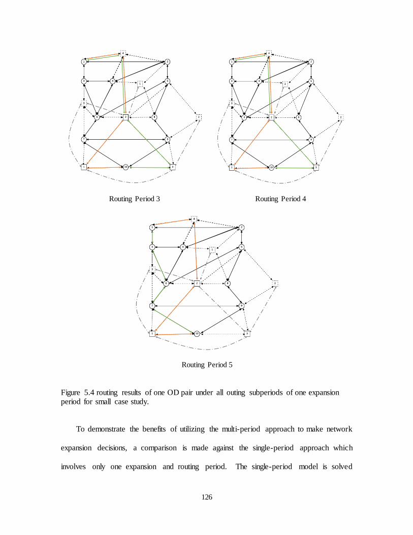
126

Routing Period 3 Routing Period 4

Routing Period 5

Figure 5.4 routing results of one OD pair under all outing subperiods of one expansion period for small case study.

To demonstrate the benefits of utilizing the multi-period approach to make network

expansion decisions, a comparison is made against the single-period approach which

involves only one expansion and routing period. The single-period model is solved

127

considering all OD pairs for different periods of the original problem and assumed the

worst case scenario: highest demand and smallest time windows for corresponding OD

pairs. It also considers the highest disruption percentages for links and terminals for all

scenarios. The reason behind this approach is to emulate a manager’s decision to expand

the network to accommodate the worst case scenario within the planning period. The

budget for the single-period model is the sum of the budget of all expansion periods of the

original problem. The solution to the optimal single-period model involves opening two

new terminals at candidate nodes 2 and 3 at the beginning of the planning horizon.

Candidate terminal 2 is also selected under the multi-period case; however, it will not be

opened until the second expansion period. The multi-period approach outperforms the

single-period one in three folds. It reduces the total routing cost by 18%, increases capacity

utilization by 5%, and reduces lost demand by 15% for the entire planning horizon. Note

that the multi-period model also has the advantage of not presuming that the entire budget

is available at the beginning of the planning horizon. Accordingly, the multi-period version

of network expansion is more efficient in terms of overall cost, budget availability and

resource utilization.

5.6.2 LARGE SIZE NETWORK

In this section, RMPINEP is applied to a realistic-sized intermodal network of a railroad

company in U.S. As shown in previous section, this problem is computationally too

expensive for even small size networks with EE thus this large size network in only solved

with SA.

The network consists of a rail network of a class 1 railroad company with 20 existing

terminals which covers Midwest and Western side of the U.S. It also includes a highway

128

network of 44 major cities in the same geographic area with interstates between them. The

company decides to increase its operational capacity by opening new terminals from 10

candidate nodes, expanding its existing terminals and retroffiting weaker rail links in its

network. Candidate terminals are in a good proximity of areas with higher demand

quantities and disruptions risks. Selected terminals can serve as back up terminals in case

of disruptions and fluctuations in the demand. Figures 5.5(a) and 5.5(b) depict the

aforementioned rail and highway networks, respectively.

(a)

129

(b)

Figure 5.5 Test case network: (a) Intermodal rail network; (b) Highway network.

Highway distances and their corresponding travel times were drawn from Google

Maps. Railroad company’s website provided rail mile distances between intermoda l

terminals. Travel times on rail links were computed by assuming an average speed of 35

miles per hour for trains. A 24 hours dwell time was assumed for terminals operating 24/7

(24 hours per days, 7 days per week) and it was increased to 30 hours for terminals that

were open 24/5. There was a charge of $0.7 per mile for rail shipments and a $3.64 per

mile for truck shipments (Fotuhi and Huynh, 2016). There was also a $150 transfer cost

for containers that change mode at intermodal terminals.

The company plans to expand the network for the next 20 years over three expansion

periods at years 2020, 2025 and 2030. The expansions affect 15 annual routing periods

from 2020 to 2035. 50 to 65 different OD pairs are selected from 44 major cities in U.S.

130

and their forecasted demand quantities are drawn from Freight Analysis Framework

(FAF4) database. The origin and destination of these OD pairs are at least 750 miles apart

and their corresponding demand values are more than 125 lb per year. These two

conditions are required to make shipments eligible for intermodal shipping option (Fotuhi

and Huynh, 2015). FAF4 includes forecasted freight volumes between different zones

within U.S for every five years from 2015 to 2045. There is no information available for

the forecasted demand of routing periods between expansion periods. Hence, the demand

scenarios for these periods are estimated based on the predicted values of demand at

expansion periods available at FAF4. Since FAF4 data are in kilo tons, they are converted

to their equivalent 40-foot Container units as they are the most standardized units for

intermodal shipping.

50 to 200 intermodal trains each carrying 100 to 200 40-foot containers pass major rail

corridors of this company per day (C Systematics, 2007). 8500 daily number of trucks

move containers on major freight highway corridors (US Department of Transportation).

Accordingly, it is assumed that the capacity of roads for freight movement can range from

1000 for rural roads to 8500 for major interstates. Annual demand of each OD pair is

divided by 365 to find their average daily demand. Accordingly, the routing subproblems

found optimal daily routes for each OD pair based on the average daily demand and

capacities of infrastructure. The annual transportation cost is then computed by

multiplying the optimal daily routing cost and number of days in a year. Unlike traditiona l

strategic location-routing studies, this method can better capture the traffic congestion

(corridor capacities) impact on routing decisions.

131

The test case considers 5, 4 and 3 disruption and demand scenarios for the first, second

and third expansion periods, respectively. The first scenario of each expansion period with

the highest chance of occurrence assumes the normal situation in which no disruption

happens in the network. Hurricane in New Orleans and Florida, earthquake in state of

Washington and Oregon, Ice storm in Midwest and tornado in Midwest are the other 4

scenarios of the first expansion period. There is a small chance of earthquake in California,

tornado in Midwest and flooding in lower part of Mississippi river in the second expansion

period. Apart from the normal situation, the third expansion period includes two more

scenarios as coastal flooding in California and ice storm in Midwest. Each disruption

scenario has the maximum severity at the beginning of its corresponding expansion period

and the severity is diminished through the routing subperiods. As an example, consider

scenario 2 of the first expansion period. The capacity of the terminal in New Orleans is

degraded by 80% due to the hurricane at the beginning of the period. For the first routing

subperiod of this expansion period (the first year), only 20% of the capacity of terminals is

available for routing of freight. Moving to the next routing period which is the second

year, the terminal is partially recovered from damages and 50% of its capacity is available

for the routing decisions. The same framework exists for the subsequent routing subperiods

of this expansion period. It is assumed that disrupted infrastructure is fully recovered by

the last routing subperiod of an expansion period. It should be noted that access to real

world freight data is not possible so the results are valid for the type of data that this paper

considered. Different assumptions in terms of number of expansion and routing periods

and problem parameters may change the results.

5.6.2.1 IMPACT OF MULTI-PERIOD PLANNING ON NETWORK REPRESENTATION

132

To investigate the impact of multiple expansion time periods on total transportation cost

and terminal’s capacity utilization, the multi-period model is compared to the single-per iod

case. Like the small case study, the single-period problem considers maximum number of

OD patterns and their corresponding demand quantities as well as maximum disruption

percentages for disrupted infrastructure over all scenarios and time periods. The expansion

budget is sum of the budget of all expansion periods.

As depicted in Figure 5.6, the optimal decision for single-period problem opens a new

terminal in Fort Smith, AR, expands terminals in Seattle, WA; Phoenix, AZ; Birmingham,

AL; Kansas City, KS; Denver, CO; Chicago, IL and Spokane, WA. It also retrofits two

rail links including Seattle-Spokane and Omaha-Chicago. However, the multi-per iod

framework with three expansion periods has a different optimal design. It opens three new

terminals in Boise, ID; Fort Smith, AR; and Jackson, MS in the first, second and third

expansion periods, respectively. Birmingham, AL; Denver, CO and Chicago, IL are the

three terminals selected for expansion at the first period. No terminal is selected for

expansion in the second period and Spokane, WA is the only expanded terminal in the third

period. Unlike the single-period design, no budget is spent to retrofit any links in the

network. These results show that a remarkable portion of the budget is spent on expanding

existing terminals rather than building new ones which is a different finding compared to

the multi-priod case. Both designs have mutual new terminals and expanded existing

terminals. However, the decisions are made in different time spans for the multi-per iod

case. It is worth mentioning that no link is retrofitted in the multi-period case due to the

low chance of disruptions which is relaxed in the single-period case.

133

To address the benefit of considering different time scales for expansion and routing,

the results of multi-period model with single time scale is compared to the ones for the

multi-period model with multiple time scales. The multi-period model with single time

scale features the following parameters. It assumes that the demand for each expansion

period is the maximum number of ODs and their corresponding quantities over the routing

subperiods of that period. The disruption percentages of each expansion period is assumed

to be the highest values over the routing subperiods of that period.

The optimal design of the multi-period model with single time scale opens terminals in

Fort Smith, AR and Jackson, MS in the second and third time periods, respectively. The

whole budget is spent to expand existing terminals in Dallas, TX; New Orleans, LA;

Birimingham, AL; Denver, CO; Omaha, NB; Chicago, IL and Billings, ID in the first

period. Terminal in Seattle, WA is the only one selected for expansion in the second

period. The remaining budget in the third period is spent to expand terminals in Billings,

MT and Denver, CO. Like the multi-period model with multiple time scales, no link is

retrofitted due to the low chance of disruptions at all periods.

a) Single-period model b) Multi-period model- multiple time scales

(LT=1)

134

c) Multi-period model- multiple time scales

(LT=2)

d) Multi-period model- multiple time scales

(LT=3)

e) Multi-period model-single time scale

(LT=1)

f) Multi-period model-single time scale

(LT=2)

g) Multi-period model-single time scale

(LT=3)

Figure 5.6 Optimal network representations of the case study.

135

5.6.2.2 IMAPCT OF MULTI-PERIOD PLANNING ON CAPACITY UTILIZATION

As depicted in Figure 5.6, a significant portion of the budget is spent to expand 7 termina ls

and open a new one in the beginning of the planning horizon for the single-period problem.

However, this additional capacity is gradually provided over multiple time periods under

the multi-period approach. Figure 5.7 depicts the average capacity utilization increase of

all open terminals under the multi-period model against the single-period ones for all

scenarios under the three expansion periods. In average the daily utilization is increased

by 1 to 2 percent. This is reasonable since the multi-period model can better accommodate

the continues change in the demand over the planning horizon. Instead of providing extra

capacity within a short time (traditional single-period model), the multi-period model adds

the extra capacity in the appropriate infrastructure and period. A daily 1% increase can

generate a huge revenue for the whole planning horizon. Consider a terminal with a

capacity of handling 5000 containers daily. A 1% increase means handling 50 more

containers in a day, 18250 more containers in a year and 273750 more containers for the

whole planning horizon. If each container can produce 150$ revenue for the intermoda l

service provider, the total opportunity revenue for the company is about 40 million dollars.

Note that the case study is only considering 50 OD pairs within Midwest and Western part

of US. Hence, the overall capacity usage of the terminals is low. This will significantly

increase by considering all possible OD pairs in the whole US.

5.6.2.3 IMPACT OF MULTI-PERIODPLANNING ON TRANSPORTATION COST

AND ROUTING DECISIONS

The single-period model finds a conservative network that can survive worst case scenarios

with highest disruptions and maximum number of OD pairs with their highest demand

quantities over the planning horizon. This design disregards the low occurrence chance of

136

disruptions and gradual recovery of disrupted infrastructure over time. Accordingly, the

total transportation cost under this design is almost 1 billion dollars more for the whole

planning horizon which is around 50 million dollars annually compared to the multi-per iod

case with multiple time scales. In a similar situation, the multi-period model with single

time scale spends 600 million dollars more in transportation cost for the whole planning

horizon which is around 40 million dollars annually. The reason behind such an increase

in total cost is ignoring network recovery from disruptions. The gradual capacity recovery

of disrupted infrastructure can only be considered in the multi-period model with mult ip le

time scales. When facilities regain their initial capacities through the routing subperiods,

more shipments can be transported over their cheapest paths leading to lower overall

transportation cost. To clarify this fact, the routing results of one OD pair is discussed in

the following.

Figure 5.7 Capacity utilization comparison under the multi-period and the Single-period

expansion designs

The resulting routing decisions of one OD pair (Los Angeles, CA - Seattle, WA) is

depicted in Table 5.2. These routes correspond to five routing subperiods of the first

expansion period under the third scenario. As mentioned before, this scenario involves

earthquake in states of Washington and Oregon impacting terminals in Seattle and

Portland. There is a huge capacity reduction in rail and highway links within these states

137

as well. As shown in Table 5.2, 86% of the demand is routed via an alternative route

passing through nearby states with no disruptions in the first routing subperiod with highest

disruption severities. Only 14% of the flow is assigned to the shortest path of this OD pair

which included links within disrupted states. A remarkable portion of the demand is shifted

to the shortest path in the second routing subperiod due to the extensive recovery of

disrupted infrastructure. Once the disruption impact is fully resolved in the third routing

subperiod, all the flow is assigned to the shortest path for the subsequent routing subperiods

of this expansion period. These results verify the benefit of including shorter routing

periods in expansion decisions to better consider disruption impacts on routing of freight

flow over the network.

Table 5.2 Routing results for a specific OD pair under one expansion period.

Rt Routes Percent of

flow

1 Los Angeles-Las Vegas- St George- Salt Lake City- Boise- Seattle 86%

Los Angeles- Oakland- Medford- Portland- Seattle 14%

2 Los Angeles- Oakland- Medford- Portland- Seattle 73%

Los Angeles-Las Vegas- St George- Salt Lake City- Boise- Spokane- Seattle 27%




5.7 CONCOLUSIONS

This paper developed a mixed integer probabilistic robust model that addresses the

intermodal freight network expansion problem using a multi-period planning approach.

The model incorporated uncertainties in demand and supply as well as different time scales

for expansion and routing decisions. A hybrid simulated annealing algorithm was

developed to solve the developed model. The results verified the quality and time

138

efficiency of the algorithm compared to exhaustive enumeration for small-sized and large-

sized networks.

The results showed that the multi-period planning approach can significantly reduce

the total transportation cost and improve capacity utilization of intermodal termina ls

compared to the traditional single-period planning approach. They also verified that by

considering different time scales for routing and expansion decisions compared to mult i-

period planning with single time scale a lower transportation cost can be obtained. The

results also indicated that the available funds are best used to expand existing terminals or

build new ones rather than retrofit weaker links in the network due to the low assumed

probability of disruptions.

This work can be extended by incorporating correlated failures in disrupted

infrastructure which is more realistic in nature. Furthermore, the model can be generalized

to include other transport modes which is necessary if the scope extends to internationa l

freight movements. Providing a distribution free model to deal with uncertainties is another

important area that can be considered in future work. Incorporating the discounted value

of money over time is another important factor that can make the problem more realistic.

Instead of assuming the value of currency to stay constant over time, there can be a

discounted factor impacting that value.

139

CHAPTER 6: CONCLUSIONS

In this dissertation, three completed research studies are presented to address real world

criteria in intermodal freight network design and expansion. These studies present

significant cost reduction and revenue increase for intermodal service providers against

traditional models.

The primary objective of an intermodal service provider is to build a network which

can operate for a long time with less changes over its operational life. It also must provide

the maximum amount of revenue for the provider and satisfy the customer by fully meeting

its demand within a predefined delivery due date.

Including competition among intermodal service providers leads to more revenue for

a company intending to expand its existing intermodal network. Chapter 3 of this

dissertation focuses on proposing a model to find locations of new intermodal termina ls

for a railroad company which competes with companies offering the same service with

overlapping service areas. The model also encounters uncertainty in future demand to find

reliable locations which can respond to future changes of the demand immediately. A new

SA algorithm is also developed to solve larger sized instances of the model to make the

model practical for real life applications. The results from a set of random networks verify

efficiency of SA in terms of solution quality and computational time. From a practical

140

perspective, the model finds optimal number of new terminals and their locations that can

provide maximum revenue for a railroad company operating in US for the next 30 years.

Chapter 4 presents a new model for intermodal network expansion by addressing

uncertainty in both demand and supply. Supply uncertainty stems from natural or human-

made disasters that might happen in the network and can make a network element (link or

terminal) out of order or significantly reduces its capacity. So, it is important to include

these incidents when expanding an intermodal network to mitigate their possible risks. The

decisions include locations for new terminals, existing terminals to expand and rail links

to retrofit. A hybrid GA algorithm is also proposed to solve this model for large size

instances. The numerical results showed algorithm’s efficiency in finding optimal solutions

in much shorter time compared to commercial optimization solvers. Managerial insights

are also drawn from a real world case study. The results show that the company can

significantly save cost if they include disruption risks and demand uncertainties in their

expansion decisions. It also provides policy recommendations for practitioners of how to

spend a limited expansion budget while deciding where to locate new terminals, which

existing terminals to expand and which higher risk rail links to retrofit.

Chapter 5 improves the previous model by incorporating the dynamic nature of

expansion projects due to limited investment capital. The idea is to gradually expand the

network over the planning horizon which is divided into multiple periods. It also features

shorter periods for routing versus expansion due to the frequent changes in demand, cost

and network capacities which can significantly impact routing costs. The model decides

when and where to locate new terminals, expand existing ones and retrofit weak links as

well as routing of freight flow over the network. Due to the complexity of this model, a

141

SA algorithm is proposed to solve it for real size networks. The numerical results on a

small case study show the efficiency of the algorithm in terms of computational time and

optimality gap. The application of the model on a real size network verifies that the mult i-

period model leads to lower total transportation cost, higher capacity utilization with lower

loss of demand due to disruptions. The results also show the superiority of the multi-per iod

model with different time scales for routing and expansion versus a multi-period model

with identical time scales in terms of total transportation cost and capacity utilization.

The case study results recommended different practical actions for the third research

paper compared to the second one. Utilizing different robust optimization approaches

caused the different policy recommendations. The min-max regret approach assumed

identical chance of occurrence for all scenarios (Including normal situation and

disruptions) and tried to find a solution for the worst case scenario. However, the third case

assumed a more realistic situation in which the chance of disruption occurrence is very low

and the final decision is more focused on normal situation with no disruptions.

It is also important to note that the goal of this dissertation was to investigate the

impact of incorporating different real world parameters in intermodal network expansion

decisions and cost reductions. Since, real world data is not easily accessible, the case study

results are not generalizable in terms of the final designs and they depended on the data set

that was used. Different data and parameters may lead to different results. However, it is

proved that the proposed models can significantly reduce cost, improve routing decisions

and accommodate future disruptions and demand fluctuations.

142

REFERENCES

Ahuja, R.K., Magnanti, T.L., and Oril, J.B. (1993). Network Flows: Theory, Algorithms,

and Application, Prentice-Hall, New Jersey.

Aissi H, Bazgan C., and Vanderpooten D (2009) Min-max and min-max regret versions of

combinatorial optimization problems: A survey, European Journal of Operational

Research 197, 427-438.

Alander, J. (1992). On optimal population size of genetic algorithms, In: CompEuro 1992

Proceedings, Computer Systems and Software Engineering, 6th Annual European

Computer Conference. IEEE Computer Society Press, The Hague, Silverspr ing,

MD, 65–70.

Albareda-Sambola, M., Fernandez, E., and Nickel, S. (2012). Multi-period location-routing

with decoupled time scales. European Journal of Operational Research, 217, 248-

258.

Alumur, S. A., Nickle, S., and Saldanha-da-Gama, F. (2012). Hub location under

uncertainty. Transportation Research Part B, 46, 529–543.

Alumur, S.A., Nickle, S., Saldanha-da-Gama, F., and Seçerdin, Y. (2015). Multi-per iod

hub network design problems with modular capacities. Annals of Operations

Research, 1-24

An, Y., Zhang, Y., and Zeng, B. (2015). The reliable hub-and-spoke design problem:

Models and algorithms. Transportation Research Part B, 77, 103-122.

143

Arnold, P., Peeters, D., Thomas, I., and Marchand, H. (2001). Pour une localisa t ion

optimale des centre de transbordement intermodaux entre re´seaux de transport:

formulation et extensions. The Canadian Geographer, 45(3), 427–36.

Arnold, P., Peeters, D., and Thomas, I. (2004). Modeling a rail/road intermoda l

transportation system. Transportation Research Part E, 40, 255–270.

Arostegui, M.A., Kadipasaoglu, S.N., and Khumawala, B.M. (2006). An empirica l

comparison of Tabu search simulated annealing, and genetic algorithms for facilit ies

location problems. International Journal of Production Economics, 103(2), 742–754.

Ashtiani, M.G, Makui, A., and Ramezanian, R. (2013). A robust model for a leader–

follower competitive facility location problem in a discrete space. Applied

Mathematical Modeling, 37(1), 62-71.

Assavapokeea, T., Realff, M.J., Ammons, J. C., and Hsuan Hongd, I. (2008). Scenario

relaxation algorithm for finite scenario-based min–max regret and min–max

relative regret robust optimization. Computers and Operations Research, 35, 2093

– 2102.

Atamturk, A., and Zhang, M. (2007). Two-stage robust network flow and design under

demand uncertainty. Operations Research, 55(4), 662-673.

Ballis, A., and Golias, J. (2004). Towards the improvement of a combined transport chain

performance. European Journal of Operational Research,152, 420–436.

Bassan, S.H. (2007). Evaluating seaport operation and capacity analysis_ preliminary

methodology. Maritime Policy and Management: The flagship journal of

international shipping and port research, 34(1), 3-19.

http://www.sciencedirect.com/science/journal/0307904X

http://www.sciencedirect.com/science/journal/0307904X

144

Battelle. FAF3 Freight Traffic Analysis. Freight Analysis Framework Version 3 (FAF3).

Oak Ridge National Laboratory. FHWA, U.S. Department of Transportation, 2011.

Benedyk, I. V., Peeta, S., Zheng, H., Guo, Y., and Iyer, A. V. (2016). Dynamic Model for

System-Level Strategic Intermodal Facility Investment Planning. Transportation

Research Record: Journal of the Transportation Research Board, 2548, 24-34.

Ben-Tal A, and Nemirovski A (2002) Robust optimization-methodology and applications.

Mathematical modeling, 92 (3), 453-480.

Berdica, K. (2002). An introduction to road vulnerability: What has been done, is done and

should be done. Transport Policy 9, 117–127.

Bertsimas D, Brown D, and Caramanis C (2011) Theory and applications of robust

optimization. SIAM Review, 53 (3), 464-501.

Bookbinder, J.H., and Fox N.S. (1998). Intermodal routing of Canada–Mexico shipments

under NAFTA. Transportation Research Part E: Logistics and Transportation

Review, 34(4), 289–303.

Burgholzer, W., Bauer, G., Posset, M., and Jammernegg, w. (2013). Analyzing the impact

of disruptions in intermodal transport networks: A micro simulation-based model.

Decision Support Systems, 54, 1580–1586.

Cambridge Systematics, Inc. (2007). National Rail Freight Infrastructure Capacity and

Investment Study.

http://www.nwk.usace.army.mil/Portals/29/docs/regulatory/bnsf/AAR2007.pdf.

Accessed October 17, 2016.

http://www.nwk.usace.army.mil/Portals/29/docs/regulatory/bnsf/AAR2007.pdf

145

Chiranjivi, S.B. (2008). Framework for Evaluation of System Impacts of Intermodal

Terminals using Commodity Flow Data. Center for Virginia Transportation Studies

at the University of Virginia.

Cho, J.H., Kim, H.S, and Choi, H.R. (2012). An intermodal transport network algorithm

using dynamic programming-A case study: from Busan to Rotterdam in intermoda l

freight routing, Appl Intell, 36, 529–541.

Chu, P.C., and Beasley, J.E. (1997). A genetic algorithm for the generalized assignment

problem. Computers and Operations Research, 24, 17–23.

Contreras, I., Cordeau, J. F., and Laporte, G. (2011). The Dynamic Uncapacitated Hub

Location Problem. Transportation Science, 45(1), 18-32.

Contreras, I., Cordeau, J. F., and Laporte, G. (2011). Stochastic uncapacitated hub

location. European Journal of Operational Research, 212(3), 518-528.

Crainic, T.G. (1998). A Survey of Optimization Models for Long-Haul Freight

Transportation’, Publication CRT-98-67. Centre for Research on Transportation.

Cui, T., Ouyang, Y., and Shen, Z. J. (2010). Reliable facility location design under the risk

of disruptions. Operations Research, 58, 998–1011.

Cunningham V (2012) ‘ Siting of Freight Facilities’,

http://www.fhwa.dot.gov/planning/freight_planning/talking_freight/july182012tra

nscript.cfm.

D’Amico, E. (2002). West Coast Port Lockout Creates Problems for Chemical Shippers.

Chemical Week, 164, 10-10.

Daskin, M.S, Hesse, M.S, and Revelle, CH.S. (1997). α-reliable P-Minimax regret: A new

model for strategic facility location planning. Location science, 5(4), 227-246.

http://www.google.com/search?tbo=p&tbm=bks&q=inauthor:%22Centre+for+Research+on+Transportation+(Montr%C3%A9al,+Qu%C3%A9bec)%22

http://www.fhwa.dot.gov/planning/freight_planning/talking_freight/july182012transcript.cfm

http://www.fhwa.dot.gov/planning/freight_planning/talking_freight/july182012transcript.cfm

146

Dayanim, J.F. (1991). Disaster recovery: options for public and private networks.

Telecomm, 25, 48-51.

Desai, J., and Sen, S. (2010). A global optimization algorithm for reliable network design.

European Journal of Operational Research, 200,1–8.

D'ESTE, G.M., and Michael, A.P. Taylor (2003). Network vulnerability: an approach to

reliability analysis at the level of national strategic transport networks, Network

Reliability of Transport. Proceedings of the 1st International Symposium on

Transportation Network Reliability (INSTR).

Drezner, Z. (1995). Facility location-a survey of applications and methods. Berlin:

Springer.

Drezner, T., Drezner, Z., and Salhi, S. (2002). Solving the multiple competitive facilit ies

location problem. European Journal of Operational Research, 142, 138–151.

Eiselt, H.A., and Marianov, V. (2009). A conditional p-hub location problem with

attraction functions. Journal of Computers and Operations Research, 6, 3128 –

3135.

Ernst, A.T., and Krishnamoorthy, M. (1999). Solution algorithms for the capacitated single

allocation hub location problem. Annals of Operations Research, 86, 141-159.

Fotuhi, F., and Huynh, N. (2013). A new planning model to support logistics service

providers in selecting mode, route, and terminal location. Polish Maritime

Research, 20, 67-73.

Fotuhi, F., and Huynh, N. (2015). Intermodal network expansion in a competitive

environment with uncertain demands. International Journal of Industria l

Engineering Computations, 6(2), 285-304.

http://link.springer.com/search?facet-author=%22A.T.+Ernst%22

147

Fotuhi, F., and Huynh, N. (2016). Reliable Intermodal Freight Network Expansion with

Demand Uncertainties and Network Disruptions. Networks and Spatial Economics,

1-29.

Garg, M., and Smith, J.C. (2008). Models and algorithms for the design of survivable mult i-

commodity flow networks with general failure scenarios. OMEGA, 36, 1057-1071.

Gelareh, S., Nickel, S., and Pisinger, D. (2010). Liner shipping hub network design in a

competitive environment. Transportation Research Part E, 46, 991–1004.

Gelareh, S., Monemi, R., and Nickle, S. (2015). Multi-period hub location problems in

transportation. Transportation Research Part E, 75, 67-94.

Ghaffari-Nasab, N., Ghazanfari, M., and Teimoury, E. (2015). Robust optimiza t ion

approach to the design of hub-and-spoke networks. International Journal of

Advanced Manufacturing Technology, 76, 1091–1110.

Godoy, L.A. (2007). Performance of storage tanks in oil facilities damaged by hurricanes

Katrina and Rita. Journal of Performance of Constructed Facilities, 21, 441–449.

Groothedde, B., Ruijgrok, C., and Tavasszy, L. (2005). Towards collaborative, intermoda l

hub networks: A case study in the fast moving consumer goods market.

Transportation Research Part E: Logistics and Transportation Review, 41 (6), 567–

583.

Ham, H., Kim, T.J., and Boyce, D. (2005). Assessment of economic impacts from

unexpected events with an interregional commodity flow and multimoda l

transportation network model. Transportation Research Part A, 39, 849–860.

148

Hatefi, S.M., and Jolai, F. (2014). Robust and reliable forward-reverse logistics network

design under demand uncertainty and facility disruptions. Applied Mathematica l

Modeling, 38, 2630–2647.

Holland, J. (1975). Adaptation in natural and artificial systems: an introductory analysis

with applications to biology, control, and artificial intelligence, University of

Michigan Press, Michigan.

Huang, J., and Wang, Q. (2009). Robust optimization of hub and spoke airline network

design based on multi-objective genetic algorithm. Journal of transportation

systems engineering and IT, 9(3), 86-92.

Huff, D.L. (1964). Defining and estimating a trading area. Journal of Marketing, 8, 28-34.

Ishfaq. R., and Sox, C. (2010). Intermodal logistics: the interplay of financial, operational

and service issues. Transportation Research Part E: Logistics and Transportation

Review, 46(6), 926–49.

Ishfaq, R., and Sox, C. (2011). Hub location–allocation in intermodal logistic networks.

European Journal of Operational Research, 210(2), 213–230.

Johnson, D.S, Aragon, C.R, Mcgeoch, L.A., and Schevon, C. (1989). Optimization by

Simulated Annealing: an experimental evaluation; Part 1, Graph Partitioning.

Operations Research, 37(6), 865-892.

Kirkpatrick, S., Gelatt, C.D., and Vecchi, M.P (1983). Optimization By simulated

annealing. Science, 220, 671–680.

Ko, H.J., and Evans, G.W. (2007). A genetic algorithm-based heuristic for the dynamic

integrated forward/reverse logistics network for 3PLs, Computers and Operations

Research, 34, 346–366.

149

Kouvelis, P., and Yu, G. (1997). Robust discrete optimization and its applications. Kluwer,

Dordrecht.

Krumke, S.O. (2004). Nonlinear optimization. Technische Universität Kaiserslautern.

Lange, P., and Huber, S. (2015). Back casting in freight transport demand modeling-

chances and challenges. Working Paper. DLR – Deutsches Zentrum für Luft- und

Raumfahrt (German Aerospace Center). Institute of Transport Research. Berlin.

Limbourg, S., and Jourquin, B. (2009). Optimal rail–road container terminal locations on

the European network. Transportation Research (E), 45 (4), 551–563.

Lin, CH. CH., Chiang, Y., and Lin, Sh. W. (2014). Efficient model and heuristic for the

intermodal terminal location problem. Computers and Operations Research, 51,

41–51.

Liu, C., Fan, Y., and Ordonez, F. (2009). A two-stage stochastic programming model for

transportation network protection, Computers and Operations Research, 36, 1582–

90.

Lüer-Villagra, A., and Marianov, V. (2013). A competitive hub location and pricing

problem. European Journal of Operational Research, 231(3), 734-744.

Macharis, C., and Bontekoning, Y. M. (2004). Opportunities for OR in intermodal freight

transport research. European Journal of Operational Research, 153, 400–416.

Macharis, C., Caris, A., Jourquin, B., and Pekin, E. (2011). A decision support framework

for intermodal transport policy. European Transport Research Review, 3(4), 167-

178.

150

Makui, A., Rostami, M., Jahani, E.,and Nikui, A. (2012). A multi-objective robust

optimization model for the capacitated P-hub location problem under uncertainty.

Management Science Letters, 2, 525–534.

Marianov, V., Serra, D., and Revelle, C. (1999). Location of hubs in a competitive

environment. European Journal of Operational Research, 114 (2), 363-371.

Marianov, V., Serra, D. (2003). Location models for airline hubs behaving as M/D/c

queues. Computers and Operations Research, 30, 983 – 1003.

Marufuzzaman, M., Eksioglu, S.D., Li, X., and Wang, J. (2014). Analyzing the impact of

intermodal-related risk to the design and management of biofuel supply chain.

Transportation Research Part E, 69, 122–145.

Matisziw, T. C., and Murray, A.T. (2009). Modeling s-t path availability to support disaster

vulnerability assessment of network infrastructure. Computers and Operations

Research, 36, 16 – 26.

Melo, M.T., Nickel, S., and Saldanha da Gama, F. (2006). Dynamic multi-commod ity

capacitated facility location: a mathematical modeling framework for strategic

supply chain planning. Computers and Operations Research, 33, 181–208.

Meng, Q., and Wang, X. (2011). Intermodal hub-and-spoke network design: Incorporating

multiple stakeholders and multi-type containers. Journal of Transportation

Research Part B, 45, 724–742.

Miller-Hooks, E., Zhang, X., and Faturechi, R. (2012). Measuring and maximizing

resiliency of freight transportation networks. Computers and Operations Research,

39,1633–1643.

http://www.sciencedirect.com/science/journal/03772217

151

Mulvey, J.M., Vanderbei, R.J., and Zenios, S.A. (1995). Robust optimization of large-scale

systems. Journal of Operations Research, 43(2), 264-281.

Murray, A.T., and Church, R.L. (1996). Applying simulated annealing to location-planning

models. Journal of Heuristics, 2, 31-53.

Nagy, G., and Salhi, S. (2007). Location-routing: Issues, models and methods. European

Journal of Operational Research, 177(2), 649-672.

Nocera, S. (2009). A heuristic solution for the yearly capacity of an intermodal termina l.

Journal of Interdisciplinary Mathematics, 12(3), 367–393.

Orabi, W., El-Rayes, K., Senouci, A., and Al-Derham, H. (2009). Optimizing postdisaster

reconstruction planning for damaged transportation networks. Journal of

Construction Engineering and Management, 135(10), 1039–1048.

Ortiz, D., Weatherford, B., Willis, H., Collins, M., Mandava, N., and Ordowich, C. (2007).

Increasing the Capacity of Freight Transportation U.S. and Canadian Perspectives,

Rand Corporation, Sanata Monica, CA.

Peeta, S., Salman, F.S., Gunnec, D., and Wisvanath, K. (2010). Pre-disaster investment

decisions for strengthening a highway network, Computers and Operations

Research, 37, 1708-1719.

Peng, P., Snyder, L.V., Lim, A., and Lie, Z. (2011). Reliable logistics network design with

facility disruptions, Transportation Research Part B, 45, 1190–1211.

Racunica, I., and Wynter, L. (2005). Optimal location of intermodal freight hubs.

Transportation Research Part B: Methodological, 39 (5), 453–477.

Ramezani, M., Bashiri, M., and Tavakkoli-Moghaddam, R. (2013). A robust design for a

closed-loop supply chain network under an uncertain environment, The

International Journal of Advanced Manufacturing Technology, 66, 825-843.

152

Rios, M., Marianov, V., and Gutierrez, M. (2000). Survivable capacitated network design

problem: new formulation and Lagrangean relaxation, Journal of the Operational

Research Society, 51, 574–582.

Rutten, B.J.C.M. (1995). On medium distance intermodal rail transport. Ph.D. thesis, Delft

University of Technology, Delft.

Sahindis, N. (2013). Baron. Carnegie Mellon University, Department of Chemical

Engineering. http://www.gams.com/dd/docs/solvers/baron.pdf.

Santos, B. F., Limbourg, S., and Carreira, J. S. (2015). The impact of transport policies on

railroad intermodal freight competitiveness- the case of Belgium. Transportation

Research Part D, 34, 230–244.

Sarkar, P., Armstrong, C., and Hua, V. (2002). Idling time: the West Coast shutdown is

beginning to hurt workers, industries dependent on imports. San Francisco

Chronicle, B1.

Shahabi, M., and Unnikrishnan, A. (2014). Robust hub network design problem.

Transportation Research Part E, 70, 356-373.

Sirikijpanichkul, A., and Ferreira, L. (2005). Multi-objective evaluation of intermoda l

freight terminal location decisions. In Proceedings of 27th Conference: Australian

Institute of Transport Research.

Slack, B. (1990). Intermodal transportation in North America and the development of

inland load centers. Professional Geographer, 42(1), 72–83.

Snediker, D.E., Murray, A.T., and Matisziw, T. C. (2008). Decision support for network

disruption mitigation. Decision Support Systems, 44, 954–969.

http://www.gams.com/dd/docs/solvers/baron.pdf

153

Snyder, V.L., and Daskin, M. (2005). Stochastic p-Robust Location Problems. IIE

Transactions, 38 (11), 971-985.

Snyder, L. V. (2006). Facility location under uncertainty: a review. IIE Transactions,

38(7), 547-564.

Sohn, J., Kim, T.J., Hewings, G.J.D., Lee, J. S., and Jang, S.G. (2003). Retrofit priority of

transport network links under an earthquake. Journal of Urban Planning and

Development, 129(4), 195-210.

Sohn, J. (2006). Evaluating the significance of highway network links under the flood

damage: an accessibility approach. Transportation Research Part A, 40, 491–506.

Sorensen, K., Vanovermeire, CH., and Busschaert, S. (2012). Efficient Meta heuristics to

solve the intermodal terminal location problem. Computers and Operations

Research, 39(9), 2079-2090.

SteadieSeifi, M., Dellaert, N.P., Nuijten, W., Van Woensel, T., and Raoufi, R. (2014).

Multimodal freight transportation planning: A literature review. European Journal

of Operational Research, 233, 1–15.

Taghipourian, F., Mahdavi, I., Mahdavi-Amiri, N., and Makui, A. (2012). A fuzzy

programming approach for dynamic virtual hub location problem. Applied

Mathematical Modelling, 36, 3257–3270.

Tang, J., Tang, L., and Wang, X. (2013). Solution method for the location planning

problem of Logistics Park with variable capacity. Computers and Operations

Research, 40, 406–417.

Taner, M., and Kara, B. (2015). Endogenous effects of hubbing on flow intensit ies,

Networks and Spatial Economics, DOI: 10.1007/s11067-015-9314-6.



154

Taniguchi, E., Noritake, M., and Izumitani, T. (1999). Optimal size and location planning

of public logistics terminals. Transportation Research Part E, 35, 207_222.

Transportation Statistics Annual Report. (2012). U.S. Departments of Transportation,

Research 39 and Innovative Technology Administration, Bureau of Transportation

Statistics, 2013. 40

http://www.rita.dot.gov/bts/sites/rita.dot.gov.bts/files/tsar_2012.pdf.pdf. Accessed

September 29, 2016.

United Nations (Economic Commission for Europe), European Conference of Ministers of

Transport (ECMT), and the European Commission (EC). Terminology on

combined transport, New York and Geneva, 2001.

U.S. Department of Transportation Federal Railroad Administration. 2005. “Intermoda l

Transportation and Inventory Cost Model: Highway-to-Rail Intermodal (ITIC)

User’s Manual (computer software)”.

Verter, V., and Dincer, M.C. (1995). Facility Location and Capacity Acquisition: An

Integrated Approach. Naval Research Logistics, 42, 1141-1 160.

Vidovic, M., Zecevic, S., Kilibarda, M., Vlajic, J., Bjelic, N., and Tadic, S. (2011). The p-

hub model with hub-catchment areas, existing hubs, and simulation: A case study

of Serbian intermodal terminals, Networks and Spatial Economics 11, 295-314.

Viswanath, K., and Peeta, S. (2003). Multicommodity maximal covering network design

problem for planning critical routes for earthquake response, Transportation

Research Record, 1857, 1–10.

155

Woxenius, J. (2007). Generic Framework for Transport Network Designs: Applicat ions

and Treatment in Intermodal Freight Transport Literature. Transport Reviews, 27

(6), 733–749.

Yaghini, M., Momeni, M., and Sarmadi, M. (2012). A Simplex-based simulated annealing

algorithm for node-arc capacitated multicommodity network design, Applied Soft

Computing, 12, 2997-3003.

Yang, T.H. (2009). Stochastic air freight hub location and flight routes planning. Applied

Mathematical Modelling, 33, 4424–4430.

intermodal network design and expansion for freight ... · intermodal network design and expansion...

Documents