intermittent thinning of jakobshavn isbræ, west greenland ... · intermittent thinning of...

Intermittent thinning of Jakobshavn Isbræ, West Greenland,since the Little Ice Age

Bea CSATHO,1 Toni SCHENK,2 C.J. VAN DER VEEN,3 William B. KRABILL4

1Department of Geology, University at Buffalo, The State University of New York,855 Natural Sciences Complex, Buffalo, New York 14260, USA

E-mail: [email protected] of Civil and Environmental Engineering and Geodetic Science, The Ohio State University,

Columbus, Ohio 43210-1275, USA3Department of Geography and Center for Remote Sensing of Ice Sheets, University of Kansas,

2335 Irving Hill Road, Lawrence, Kansas 66045-7612, USA4Cryospheric Sciences Branch, Goddard Space Flight Center NASA/Wallops Flight Facility,

Wallops Island, Virginia 23337, USA

ABSTRACT. Rapid thinning and velocity increase on major Greenland outlet glaciers during the last twodecades may indicate that these glaciers became unstable as a consequence of the Jakobshavn effect(Hughes, 1986), with terminus retreat leading to increased discharge from the interior and consequentfurther thinning and retreat. To assess whether recent trends deviate from longer-term behavior, wemeasured glacier surface elevations and terminus positions for Jakobshavn Isbræ, West Greenland, usinghistorical photographs acquired in 1944, 1953, 1959, 1964 and 1985. These results were combined withdata from historical records, aerial photographs, ground surveys, airborne laser altimetry and fieldmapping of lateral moraines and trimlines, to reconstruct the history of changes since the Little Ice Age(LIA). We identified three periods of rapid thinning since the LIA: 1902–13, 1930–59 and 1999–present.During the first half of the 20th century, the calving front appears to have been grounded and it startedto float during the late 1940s. The south and north tributaries exhibit different behavior. For example,the north tributary was thinning between 1959 and 1985 during a period when the calving front wasstationary and the south tributary was in balance. The record of intermittent thinning, combined withchanges in ice-marginal extent and position of the calving front, together with changes in velocity, implythat the behavior of the lower parts of this glacier represents a complex ice-dynamical response to localclimate forcings and interactions with drainage from the interior.

INTRODUCTION

The Greenland ice sheet (GIS) may have been responsiblefor rapid sea-level rise during the last interglacial period(Cuffey and Marshall, 2000). Recent studies indicate that it islikely to make a faster contribution to future sea-level risethan previously believed (Parizek and Alley, 2004; Rignotand Kanagaratnam, 2006). Some of its larger outlet glaciershave accelerated to as much as double their former speeds,and have thinned by tens of meters per year during the last5–15 years (Thomas and others, 2000, 2003; Joughin andothers, 2004; Thomas, 2004). Recently, Rignot and Kanagar-atnam (2006) documented major increases in ice dischargeon many of the outlet glaciers draining the interior. Theserecent changes may, in part, reflect adjustment to recentwarming trends, but these alone cannot explain ongoingrapid thinning, and most of the outlet glaciers appear to beundergoing ice-dynamical changes (Thomas and others,2000, 2003; Van der Veen, 2001; Thomas, 2004; Rignot andKanagaratnam, 2006). The response of these outlet glaciersto climate change can occur much more rapidly than that ofthe interior ice, and can therefore contribute to short-termchanges in sea level. Moreover, rapid thinning of peripheraloutlet glaciers has been proposed by Hughes (1986, 1998)as an initiator of increased discharge of interior ice, withpotentially severe impacts on coastal communities through arise in global sea level as more ice is discharged into the

oceans. Consequently, it is important to investigate possiblecauses for ongoing rapid changes in order to understandhow the GIS may respond to future climate change.

So far, few studies have investigated the significance ofthe recent rapid changes of Greenland outlet glaciers withinthe broader context of retreat since the Last GlacialMaximum (LGM) and, more significantly, retreat followingthe temporary glacier advance during the Little Ice Age (LIA)(Weidick, 1968; Ten Brink, 1975; Forman and others, 2007).Moreover, long-term records of outlet glacier change areusually based on time series of calving-front positions(Weidick, 1968, 1991, 1995). Such records can be mislead-ing on tidal glaciers, whose floating terminus can eitheradvance or retreat without any substantial changes fartherup-glacier. For example, Sohn and others (1998) inferredlarge seasonal variations in the position of the calving frontof Jakobshavn Isbræ, postulated to be associated withsurface ablation. A more comprehensive record thatincludes long-term time series of surface elevation, calv-ing-front and ice-marginal position and ice-velocity changesis needed to assess the significance of recent changes and toprovide input for modeling studies.

Jakobshavn Isbræ is the major drainage outlet on the westcoast of Greenland, draining approximately 7% of the icesheet. Rignot and Kanagaratnam (2006) report that the fluxdischarge increased from 24 km3 a–1 in 1996 to 46 km3 a–1 in2005. Repeat airborne laser altimeter surveys along a

Journal of Glaciology, Vol. 54, No. 184, 2008 131

120 km long profile, conducted almost every year over thenorthern part of the glacier since 1991, indicate thatthickening prevailed from 1991 to 1997, followed by morerecent thinning, reaching several meters per year 20 km up-glacier from the terminus, and lower thinning rates fartherinland (Thomas and others, 2003). On a longer timescale,the position of the calving front retreated �25 km up thefjord to 5 km seaward from the grounding line over theperiod 1850–1950 (Weidick, 1995). Subsequently, the calv-ing front remained stationary, with annual oscillations of�2 km around the stable position (Sohn and others, 1998). Inrecent years, however, the terminus position has retreatedand is currently near the grounding line (Weidick and others,2004; Joughin, 2006). Clearly, these observations indicatemajor ongoing changes in this principal drainage route forinland ice.

The unresolved question is whether the ongoing thinningand retreat are unusual or, perhaps, a manifestation oflonger-term behavior of the ice sheet, such as recovery fromthe general warming following the LIA maximum glacierextent and thickness. To address this question, a history ofsurface elevations is needed. While terminus positions mayoffer a general picture of glacier behavior, they cannot beused to accurately reconstruct the history of mass changes,since during much of its retreat the terminus was likely tohave been floating and thus susceptible to small and short-lived climate perturbations. For the Jakobshavn region, theinstrumental record dates back to aerial photographyconducted by Kort- og Matrikelstyrelsen (KMS; DanishNational Survey and Cadastre) in the 1940s. We use thesephotographs to reconstruct time series of surface-elevationchanges between the 1940s and 1985. Glacier historiesextending farther back in time must be based on glacialgeomorphological information retrieved from formerlyglaciated regions. With the objective of reconstructing the

glacier history over the last two centuries, a field camp wasestablished on the northern margin of Kangia Isfjord, close tothe head of the fjord, on the eastern end of Nunatarsuaq(‘Great Nunatak’), just above the trimline (Fig. 1). This,Camp-2, was occupied for several days during July 2003, toestablish a retreat sequence, to map fresh lateral morainesand to provide field-based validation for trimline mappingfrom multispectral satellite images (Csatho and others, 2005;Van der Veen and Csatho, 2005).

The objective of this paper is to provide a longer-termrecord for the Jakobshavn drainage basin and to place recentchanges in the broader context of retreat since the LIA. Tothis effect, we employ a suite of data and measurementtechniques, as well as observations reported earlier in theliterature, to derive the first quantitative history of elevationchange of the lower part of Jakobshavn Isbræ. This record iscompared with climate data from the nearby coastal stationat Ilulissat airport to discuss possible causes for the observedintermittent thinning since the LIA.

PHOTOGRAMMETRIC MEASUREMENTSTo unravel the complex pattern of thinning that followed theLIA, surface elevations over a large part of Jakobshavn Isbræshould be precisely measured at regular time intervals.Surface elevations along a few trajectories have beenrepeatedly measured since the early 1990s by NASA’sAirborne Topographic Mapper (ATM) laser altimetry system(Thomas and others, 1995, 2003; Thomas, 2004). However,these measurements refer only to the last 15 years and theyshould be placed in a broader temporal context to assesstheir significance and evaluate the longer-term behavior.This section provides a summary of available data,comments on previous work and describes the data selectedand the measurements performed for this study.

Fig. 1. (a) Orthophotograph of Jakobshavn Isbræ with geographic and glaciological features and transects. Photograph taken on 9 July 1985,provided by KMS, Denmark. (b) Location of Jakobshavn drainage basin on shaded-relief digital elevation model of Greenland. Coordinatesin Universal Transverse Mercator projection system (Zone 22) are given outside the image.

Csatho and others: Intermittent thinning of Jakobshavn Isbræ132

Available data and previous workA wealth of geospatial information is available about theevolution of the terminus position, extent and ice motion ofJakobshavn Isbræ. Terrestrial photographs, paintings, verbaldescriptions and books provide the earliest observations(e.g. Hammer, 1883; Koch and Wegener, 1930). Note that inthis paper, a distinction is made between terminus positionand ice-marginal extent, with the latter referring to theposition of the land-based ice margin in the regions northand south of Kangia Isfjord (Jakobshavn Isfjord).

The first photogrammetric survey in the Jakobshavn regionwas conducted during the 1930s to create 1 : 250 000 scaletopographic maps (Weidick, 1968). Subsequent regionalsurveys covering Jakobshavn Isbræ include acquisition ofTrimetrogon aerial photographs by the US Air Force duringand immediately after World War II, and repeat surveys ofthe catchment basins of all major outlet glaciers between 688and 728N in 1957–58 and 1964 as part of the ExpeditionsGlaciologiques Internationales au Groenland (EGIG) (Bauer,1968; Carbonnell and Bauer, 1968). Additional verticalaerial photographs were collected in the 1940s, 1953 and1959 (Weidick, 1968). Finally, a comprehensive coverage ofthe ice-free coastal areas of Greenland was obtainedbetween 1978 and 1987. KMS performed a rigorous aerialtriangulation with this photography, using control pointsestablished by GPS (global positioning system) measure-ments. Table 1 lists aerial photography collected at varioustimes between 1940 and 1990. The table also containsrelevant information about these diverse photographicmissions. Most of the photography and related metadata,such as camera calibration protocols, are archived by KMS.

The primary purpose of these aerial surveys was to createand update maps. The photographs were also used to deter-mine the fluctuation of the terminus position of JakobshavnIsbræ, to map advance/retreat along the ice-sheet margin andto estimate thinning since the LIA by measuring elevationdifference between the trimline and the ice-sheet boundary(Weidick, 1968, 1969, 1995). As part of the EGIG program,Bauer (1968) and Carbonnell and Bauer (1968) determinedice velocities along profiles across the fjord using repeataerial surveys from 1958 and 1964. Finally, comprehensivestudies of ice velocities and elevations were undertaken withrepeat photography obtained in 1985–86 (Fastook andothers, 1995; Johnson and others, 2004).

All these previous studies were carried out using localreference systems that were not well documented, if at all.Moreover, most results are published in the form of hard-copymaps, and no digital datasets are available. Thus, it is verydifficult to compare these results. Consequently their use forlong-term change detection is unfortunately rather limited.

Selected aerial photographs and scanningWe obtained diapositives and metadata from five aerialsurveys from KMS. Figure 2 shows the flight-lines andexposure centers and Table 2 contains relevant information.Although aerial photographs might have been acquired priorto the A44 mission, we have so far been unsuccessful inlocating these older photographs. This logistic problem isnot unique, as it is increasingly difficult to locate historicalphotographs and obtain the technical information necessaryto render them useful for quantitative analysis and changedetection, as knowledgeable people retire. Another oddity isthe date of mission A44; no metadata are available nor is a

date printed on the film (as is customary). Based oncircumstantial evidence, we tentatively assigned a date of1944, but this must still be verified.

In order to apply some image processing and to makemeasurements on digital photogrammetric workstations(soft-copy workstations), we converted the diapositives todigital images with our RasterMaster photogrammetricprecision scanner. We selected a suitable pixel size basedon the film quality (mainly its resolution). It is important toadequately represent the inherent film resolution to allowidentification of fine details on the digital images. This iscrucial for orienting images of different epochs. Table 2 liststhe pixel size and its associated ground sampling distance.

Orientation of historical photographsFor change detection it is an absolute prerequisite toestablish a common three-dimensional (3-D) referenceframe for all sensory input data, such as images obtainedby different camera systems, profiles measured by laseraltimetry or elevations obtained from local surveys. Themajor technical challenge in using historical photographyfor change detection is the orientation of images obtainedfrom different missions. This entails the determination of thecamera’s perspective center and its attitude during the timeof exposure. The classic approach of using ground-controlpoints (GCPs) poses a problem for a number of reasons. Forinstance, it is nearly impossible to obtain reliable informa-tion about GCPs used to orient historical photographybecause they are usually defined in poorly documentedlocal reference systems. Although it is possible to determineGCPs now with GPS, the cost of field campaigns to remoteareas is prohibitive. Therefore we have established thenecessary control points photogrammetrically, briefly de-scribed below.

Of the five selected sets of aerial photographs, the 1985mission is of particular interest because it is oriented to theWorld Geodatic System 1984 (WGS84) reference frame byway of aerial triangulation, using control points measured by

Table 1. List and availability of aerial photographs collected overJakobshavn Isbræ since the 1940s. Bold dates indicate aerial photo-graphs used in this study. OAP: oblique aerial photograph; NL: notlocated yet; VAP: vertical aerial photograph; TAP: Trimetrogonaerial photograph; IGN: Institut Geographique National, France;Kucera: Kucera International Inc., Dayton, OH, USA

Date Camera Origin Source

1931 OAP NL Weidick (1968)1942 NL Mikkelsen and Ingerslev (2002)1944? VAP KMS Personal communication from

A. Nielsen (2005)6 Aug 1946 TAP KMS Weidick (1968)1948 NL Weidick (1968)3 Jul 1953 VAP KMS Weidick (1968)1957 NL Mikkelsen and Ingerslev (2002)15, 19 Jul 1958 VAP IGN Bauer (1968)26 Jun 1959 VAP KMS Weidick (1968)29 Jun 1964 VAP KMS Carbonnell and Bauer (1968)12 Jul 1964 VAP KMS Carbonnell and Bauer (1968)10, 24 Jul 1985 VAP Kucera Fastook and others (1995)9 Jul 1985 VAP KMS Personal communication from

A. Nielsen (2005)7, 23 Jul 1986 VAP Kucera Fastook and others (1995)

Csatho and others: Intermittent thinning of Jakobshavn Isbræ 133

GPS. The results, including the control points and exteriororientation data, are available from KMS. As NASA’s repeatlaser altimetry missions are recorded in the same system, itmakes sense to use WGS84 as the common reference frame.

To orient the older photographs (1944–64) used in thisstudy, we proceed as follows. Identical point features in the1985 and older photographs are manually identified andmeasured. With the available orientation data it is possible todetermine the 3-D location of these measured points in the1985 photography with respect to the WGS84 referenceframe. This renders the necessary GCPs for orienting the olderphotography to the common reference system, performing abundle block adjustment. The procedure is summarizedbelow, and Table 3 contains the most relevant results.

Measure identical point features in 1985 and photog-raphy from earlier flight.

Compute 3-D position of measured points in 1985photography in WGS84 system.

Perform aerial triangulation with the earlier flight, usingpoints from previous step as GCPs.

Surface elevations in oriented earlier flight are now inWGS84 reference system.

Using a block adjustment for orienting older photographsoffers several advantages, among them the possibility offormally assessing the accuracy of the results. The variancecomponent, �0, indicates the measurement accuracy. Undergood circumstances one can expect an rms (root-mean-square) error of �1pixel, corresponding to 1–2m. Theactual errors are larger (see Table 3), which is not surprising,considering the rather poor image quality and unaccountedfilm distortions of historical photographs. The accuracy ofpoints and the exterior orientation parameters are formallyobtained from the variance–covariance matrix. Rather thanlisting all individual point errors we determined an averagerms error. This is mainly influenced by the number anddistribution of GCPs and their accuracy. The results inTable 3 confirm the success of our orientation method. Theplanimetric rms error of an arbitrary point is less than 3mand just about 4m for elevations.

Profile measurementsAs outlined earlier, NASA has repeated laser altimetrymissions along the profiles shown in Figure 1 since theearly 1990s. Our goal was to determine ice elevations at thesame locations on old photographs. We performed thisoperation manually on a soft-copy workstation, as brieflydescribed here.

With the orientation data now established for historicalphotography, one can set up a stereo model on the soft-copyworkstation. The models are absolutely oriented with respectto WGS84, the common reference frame for this project.Any 3-D point can be projected to the two images of thestereo model, mathematically emulating the image-forma-tion process. The soft-copy workstation allows the cursor tobe positioned in both images on the projected image pointsand automatically centers the displayed sub-images at theselocations. If the projected 3-D point is on the visible surfaceof that stereo model then the operator perceives the cursorlocation in three-dimensions right on the surface.

We now employ this principle for measuring elevationsalong the ATM profiles. The ATM profile points are projectedto the stereo model. Because the ice surface changedbetween ATM and aerial flights, the projected ATM pointsare not on the visible surface and the operator must find theice surface by moving the measuring mark up and down at

Table 3. Results from orienting historical photographs by bundleblock adjustment

Flight-line

A44 A66 237F 272C

No. of images 5 5 4 3No. of GCPs 15 11 11 10No. of tie points 15 15 12 9rms error X (m) �2.9 �2.1 �1.9 �2.2rms error Y (m) �3.1 �2.5 �2.1 �2.7rms error Z (m) �3.6 �3.5 �3.1 �3.7

Table 2. Information about aerial photographs used in this study.GSD: ground sampling distance

Flight-line

A44 A66 237F 272C 886M

Year 1944? 1953 1959 1964 1985Photo scale 1 : 40 000 1 : 39 500 1 : 56 000 1 : 51 000 1 : 156 000Camera info. No Yes No Yes YesPixel (mm) 25 25 25 25 12GSD (m) 1.0 1.0 1.4 1.3 1.9

Fig. 2. Index map of aerial photogrammetry flights, shown on aLandsat Enhanced Thematic Mapper Plus (ETM+) satellite imageacquired on 7 July 2001. Colors denote the year of data acquisition(green – 1944?; purple – 1953; magenta – 1959; orange – 1964;red – 1985), and circles mark the exposure centers of aerialphotographs.


the projected location. For the operator to see stereoscopi-cally, good image contrast must exist around these points.Since this is not always the case, the operator moves withinthe profile direction or slightly across until satisfactoryconditions are found. Once the cursor is on the ice surface,the position is recorded. The operator then proceeds to thenext profile point.

The elevation accuracy of the profiles can be derivedtheoretically by way of error propagation, taking intoaccount measurement and interpretation errors, as well asorientation errors. This leads to an rms error in elevation ofabout �3.8m.

ANCILLARY MEASUREMENTSTrimline elevationThe highest ice-elevation stand reached during the LIA isreadily observed in the field as a sharp boundary, called thetrimline, separating vegetated terrain and rocks that werestripped bare of any vegetation during glacier advance. Thistrimline can be mapped using multispectral satellite imagesbecause exposed bedrock and freshly deposited sedimentshave distinctly different spectral-reflectance characteristicsto surfaces covered with vegetation or lichens. Csatho andothers (2005) applied surface classification procedures toLandsat Enhanced Thematic Mapper Plus (ETM+) images todistinguish between the trimline zone and other surfaceclasses (such as different snow facies, lichen and vegetation-covered surfaces, and open water). The authors identified14 different surface classes based on their spectral signature.Figure 3 shows a simplified classification map indicating themajor surface covers, which clearly distinguishes therecently exposed surfaces devoid of lichens and vegetationfrom surfaces that deglaciated earlier. The inland boundaryof the region classified as ‘trimzone’ corresponds to theposition of the LIA trimline.

Although spatial changes in margin position can bedetermined accurately by classification of multispectralimagery, elevations are needed to assess the associatedlowering of the ice surface and related ice-volume loss. Wemeasured trimline elevations manually on a soft-copyworkstation from 1985 aerial photographs. Fresh rock andmoraine surfaces are usually brighter than lichen-covered

older rock surfaces, and trimzones are therefore character-ized by light tones on black-and-white aerial photographs orvisible bands of satellite imagery (e.g. Fig. 4a). This bright-ness contrast, together with changes in image texture, formsthe basis of the traditional measurement of trimline elevationusing photo-interpretation. To aid the identification oftrimlines, we projected the boundaries of the trimzone fromthe classification map, shown in Figure 3, onto the aerialphotographs. This multisensor approach, using both theclassification of multispectral satellite imagery and visualclues, such as image brightness and texture from black-and-white stereo photographs, resulted in a robust and accurate3-D mapping of the trimlines. Trimline elevation wasmeasured along both sides of Kangia Isfjord. Figure 6 showsa segment along Nunatarsuaq.

Lateral morainesA closer inspection of the trimzone near Camp-2 onNunatarsuaq revealed a succession of lateral moraines; aclose-up of a morainal ridge is shown in Figure 4b. Theselateral moraines are believed to have been formed duringperiods of interrupted thinning, and can thus be used to inferthe history of intermittent surface lowering. To map thesemoraines, we measured surface elevations along a profileline (Fig. 4a, transect EE’). Figure 4c shows the resultingelevation profile. As discussed later in this section, thesemeasurements produced accurate elevations of lateral mo-raines and other glacial geological features. However,assigning dates to these elevations proved to be a majorchallenge. Lichenometry was attempted, but the sparselichen cover below the trimline prevented establishment ofa statistically significant lichen-growth curve. Moreover,calibration of lichen growth could only be accomplishedusing surfaces of known exposure in the town of Ilulissat,�60 km west, at the mouth of the fjord where conditions forlichen growth are likely to be very different to those close tothe ice margin. Therefore, dating of the lateral moraines,marked by bold numbers along the profile shown inFigure 4b is based on results from aerial photographs andother data presented here.

To accurately map elevations along the profile extendingfrom the trimline to the ice surface, differential carrier-phase GPS data were collected along the profile on 22 July

Fig. 3. Trimline zone around Jakobshavn Isbræ from supervised classification of multispectral Landsat ETM+ imagery acquired on 7 July2001 (modified from Csatho and others, 2005).


2003, using Javad GPS receivers (on loan from the Centerfor Mapping at The Ohio State University). Static GPSstations were surveyed at stations 100, 103 and 104, andkinematic GPS surveys with an observation every 30 s wereconducted along a trajectory connecting all numberedstations along the transect. A local GPS base station wasrunning simultaneously at station 120, near the camp, forthe entire duration of the transect survey. The GPS datawere processed by GPSurvey (Trimble Inc.). First, theposition of the base station was computed with respect tothe International GNSS Service (IGS) station operating inKellyville, near Kangerlussuaq airport, �250 km south ofJakobshavn Isbræ (GPS observations and precise position ofKellyville, as well as precise satellite orbits, from IGS).Next, the static and kinematic surveys were processedrelative to the local base station. The estimated accuracy forthe static survey is better than 5 cm, slightly worse for thekinematic survey.

Positions of stations 109 and 113–19 were determinedusing a Toshiba total station, comprising an electronictheodolite (10 arcsec accuracy) and an electronic distance-measurement unit (0.05m accuracy). The instrument was setup at the base station (120) and at stations 109 and 116.From these three stations, the other sites were determined bymeasuring point vectors. The point accuracy of �0.35mwas determined using error propagation from redundantobservations in the triangle formed by stations 120, 109and 116.

Terminus positionsTo augment the record of terminus positions presented bySohn and others (1998), positions measured on new data(aerial photographs, Landsat ETM+ and Advanced Space-borne Thermal Emission and Reflection Radiometer (ASTER)satellite imagery) or inferred from more recent laser altim-etry data have been added. A summary of these positions isgiven in Table 4.

RESULTS

Terminus positionAt the termination of the LGM, the ice margin retreated froman advanced position near the western end of Disko Island,�150 km west of the mainland coast at Ilulissat, to themouth of Kangia Isfjord. A submarine moraine shoal, alsocalled Isfjeldbanken (the iceberg bank), provided a tem-porary semi-stable terminus position (Fig. 5a; Weidick,1992; Long and Roberts, 2003). Retreat from the mouth ofthe fjord started �8000 BP at a rate of �20ma–1 (Weidick,1992). During the Holocene climatic optimum, �4000–5000 BP, the calving front was at the current position at thehead of the fjord, or perhaps even farther inland (Weidickand others, 1990, 2004; Weidick, 1992). The timing of thetermination of this retreat has been inferred from occur-rences of marine shells in the neoglacial moraines surround-ing Tissarissoq at the western side of the ‘Ice Bay’ (Fig. 5a),

Fig. 4. (a) Aerial photograph acquired in 1964 showing transect starting at Camp-2, perpendicular to Jakobshavn Isbræ on the southern slopeof Nunatarsuaq (for location see Fig. 1: EE’). Circles mark stations where geomorphologic features were mapped; numbered stations withbold circles are located on morainal ridges. (b) Photograph showing a morainal ridge at station 103. (c) Elevations along Camp-2 transect. Allstations, up to 117, are numbered and bold numbers mark stations where lateral moraines are mapped. Elevations measured along thetransect are also marked.


and from radiocarbon dating of a walrus tusk collected at�60m above present-day sea level, yielding an age of4290� 100 BP (Weidick, 1992). According to Hammer(1883) (referred to by Weidick and others, 2004), locallegends suggest that this area used to be free of ice, servingas hunting grounds. This would imply that progress of thecalving front to a more advanced position, �25 km west ofIlulissat, may have been as recent as during the LIA(AD 1500–1900) (Weidick and others, 2004).

The first to conduct scientific observations on JakobshavnIsbræ was H. Rink, who traveled by sledge to the southernside of the calving front in April 1851 and visited the northside later that year (Rink, 1857). According to his maps, theglacier terminus extended just beyond the western edge ofNunatarsuaq. Since then, the position of the terminus hasbeen observed quite frequently, first through direct obser-vations, then by aerial photography and, more recently,using satellite imagery. Figure 5a shows terminus positionssince the LIA maximum advance.

Engell gave a review of the 19th-century observations(Engell, 1903), while Georgi (1959) and Weidick (1968)

discussed observations in the first part of the 20th century. Itshould be noted here that Weidick (1968) included theobservation of Nordenskiold (1870) who claimed to haveobserved a terminus position more advanced than thatreported by Rink, which would imply a slight terminus

Table 4. Terminus positions of Jakobshavn Isbræ since 1946.Calving-front position is measured up-glacier, at the middle of thefjord, relative to western boundary of the Tissarissoq Ice Bay (Fig. 5).Bold numbers mark terminus positions determined in this study.D: day of the year, starting on 1 January; MD: modified day of theyear, Dþ 365 for D< 100; CF: calving front position; AP: aerialphotograph; TAP: Trimetrogon AP; DISP: declassified intelligencesatellite photograph; ATM: Airborne Topographic Mapper;Landsat: Landsat ETM+; SAR: synthetic aperture radar. ATMmeasurements along profile AA0

Date Sensor D/MD CF Source

km

6 Aug 1946 TAP 218/218 4.65 Weidick (1968)3 Jul 1953 AP 184/184 3.76 Weidick (1968)19 Jul 1958 AP 200/200 4.7 Bauer (1968)26 Jun 1959 AP 177/177 3.531 May 1962 DISP 121/121 3.38 Sohn and others (1998)29 Jun 1964 AP 180/180 3.02 Carbonnell and Bauer (1968)12 Jul 1964 AP 193/193 3.95 Carbonnell and Bauer (1968)9 Jul 1985 AP 190/190 5.0310 Jul 1985 AP 191/191 6.1 Fastook and others (1995)24 Jul 1985 AP 205/205 5.71 Fastook and others (1995)7 Jul 1986 AP 188/188 5.12 Fastook and others (1995)30 May 1988 SAR 150/150 3.32 Sohn and others (1998)12 Sep 1991 ATM 255/255 4.81 Sohn and others (1998)5 Feb 1992 SAR 36/401 3.79 Sohn and others (1998)3 Mar 1992 SAR 62/427 4.85 Sohn and others (1998)21 Mar 1992 SAR 80/445 4.49 Sohn and others (1998)22 Apr 1992 ATM 112/477 2.5 Sohn and others (1998)20 Aug 1992 SAR 232/232 5.65 Sohn and others (1998)9 Jul 1993 ATM 190/190 4.13 Sohn and others (1998)14 Oct 1993 SAR 287/287 5.98 Sohn and others (1998)26 May 1994 ATM 146/146 2.07 Thomas and others (2003)16 Jun 1994 ATM 167/167 1.8119 May 1995 ATM 139/139 1.7624 May 1995 ATM 144/144 2.57 Thomas and others (2003)25 May 1995 ATM 145/145 2.628 Apr 1996 SAR 98/463 3.58 Sohn and others (1998)13 May 1997 ATM 133/133 1.85 Abdalati and Krabill (1999)17 May 1997 ATM 137/137 1.85 Thomas and others (200319 May 1997 ATM 139/139 1.79 Abdalati and Krabill (1999)15 Jul 1998 ATM 196/196 5.5921 May 1999 ATM 141/141 6.42 Thomas and others (2003)17 Mar 2001 Landsat 76/441 2.984 May 2001 Landsat 124/489 1.9823 May 2001 ATM 143/143 3.197 Jul 2001 Landsat 188/188 5.764 Mar 2002 Landsat 63/428 2.8929 Mar 2002 Landsat 88/453 3.7828 Apr 2002 Landsat 118/483 2.8823 May 2002 Landsat 143/143 5.4931 May 2002 ATM 151/151 5.4617 Jun 2002 Landsat 168/168 4.651 Jul 2002 Landsat 182/182 9.123 Sep 2002 Landsat 246/246 8.7923 Mar 2003 Landsat 82/447 9.811 May 2003 ATM 131/131 11.4 Thomas (2004)28 May 2003 ASTER 148/148 12.8527 Jun 2004 ASTER 178/178 16.76 Aug 2006 Landsat 218/218 17.1

Fig. 5. Fluctuation of terminus position of Jakobshavn Isbræ.(a) Long-term retreat between 1850 and 2003 shown on a LandsatETM+ image acquired 7 July 2001 (terminus positions from Georgi(1959) and from this study). Hatched area shows calving frontlocation between 1946 and fall 1998. Twenty-first-century posi-tions are 2001 Su.: 7 July 2001 (green); 2002 Su.: 3 September 2002(orange), 2003 Sp.: 23 March 2003 (cyan) and 2004 Su.: 27 June2004 (blue). (b) Seasonal variation of terminus positions listed inTable 4, shown as function of the day of the year. Terminus positionis relative to the western boundary of the Ice Bay. Red shows thebest-fit curve to data points from 1946–98, green to points from1999–2002 and blue to points after 2002.


advance over the period 1850–70. However, according toEngell (1903), the observations made by Nordenskiold are oflittle value because he could not observe the glacierterminus and his writings do not contain sufficient informa-tion to allow for a reconstruction of the terminus position.For this reason, this position is not included in Figure 5a.

The terminus occupied a quasi-stable position between1946 and 1998 that is believed to be related to a rise of thechannel floor, as well as a pronounced bedrock protuber-ance, the ‘Ice Rumple’, in the Tissarissoq Ice Bay (Clarke andEchelmeyer, 1996). The topographic high, marked inFigure 1, rises from the bottom of the fjord to �400–550mbelow sea level (Echelmeyer and others, 1991) and acts asan important pinning point. As noted by Engell (1903) andSohn and others (1998), the position of the calving frontfluctuates on a seasonal basis around the average position.Using all available terminus positions (summarized inTable 4), the seasonal variation in calving-front positioncan be investigated further by plotting it as a function of time(Fig. 5b). Note that the position is measured in the up-glacierdirection from the western boundary of the Ice Bay, asmarked in Figure 5a. The data shown in Figure 5b can bedivided into three groups: those applying to the periods1946–98, 1999–2002 and after 2002. This grouping reflectsthe general trend of a prolonged period of a more-or-lesssteady terminus during the second half of the 20th century(1946–98), the initial period of thinning of the floatingterminus (1999–2002) and its retreat to the head of the fjord(2003–present). Starting in 1999, the magnitude of thesummer retreat increased from �4 km (Fig. 5b, red curve) to7 km (green curve). During the winter months the terminusstill advanced to its quasi-stable position, however. The last

winter advance of the quasi-stable period took place inMarch 2002, followed by a period of continuous break-upand recession of the calving front by an additional 10 km tothe head of the fjord (Fig. 5a and b, blue curve). By May2003, a major retreat had occurred and the glacier segmentin the Tissarissoq Ice Bay had become isolated and hadpartially disintegrated; most of the floating part surveyed byEchelmeyer and others (1991) has been replaced by a mix oficebergs and sea ice.

Seasonal variations in terminus position are similar tothose reported by Sohn and others (1998), with terminusretreat starting around the end of April, followed by advancestarting in late summer/early fall. Assuming a constant icevelocity of 7 kma–1, the authors inferred that the calving rateduring summer is almost six times that during winter. Theassumption of constant ice velocity throughout the year wasbased on observations reported by Echelmeyer and Harrison(1990), but this may not be applicable to more recent times.Zwally and others (2002) observed increased ice dischargefollowing surface-melt events, which would suggest greaterice speeds during late spring and summer. Indeed, Luckmanand Murray (2005) detected seasonal variations in surfacevelocity in 1995, and observations of Truffer and others(2006) revealed several speed-up events in 2006. If Jakobs-havn Isbræ is now subject to seasonal variations in glacierspeed, Figure 5b suggests that summer calving rates must beexceptionally large to cause terminus retreat in spite ofmaximum forward ice motion.

Surface elevationWe investigated the overall pattern of surface change since1944 by comparing surface elevations derived from repeat

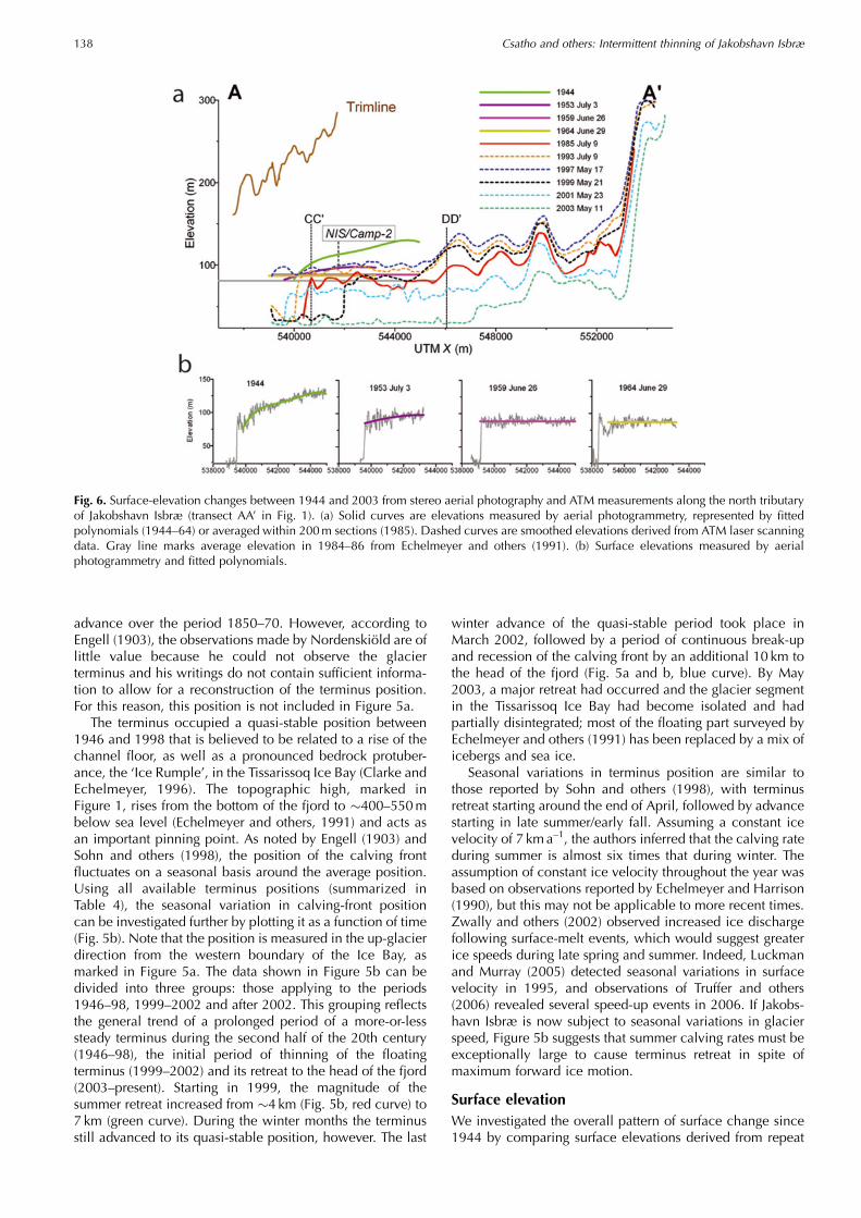
Fig. 6. Surface-elevation changes between 1944 and 2003 from stereo aerial photography and ATM measurements along the north tributaryof Jakobshavn Isbræ (transect AA’ in Fig. 1). (a) Solid curves are elevations measured by aerial photogrammetry, represented by fittedpolynomials (1944–64) or averaged within 200m sections (1985). Dashed curves are smoothed elevations derived from ATM laser scanningdata. Gray line marks average elevation in 1984–86 from Echelmeyer and others (1991). (b) Surface elevations measured by aerialphotogrammetry and fitted polynomials.


aerial photogrammetry and from airborne laser scanningalong the two longitudinal and two transverse profilesshown in Figure 1. These profiles follow trajectories of ATMlaser scanning measurements, repeatedly flown by NASAsince the early 1990s. Elevations have been measured alongprofile AA’ almost every year, but the other profiles weresurveyed only two or three times between 1993 and 2004.To generate the profiles shown in Figures 6–9, first theaverage elevations within �70m by 70m sections of theATM laser altimetry swaths are determined by fitting planarsurface patches (‘platelets’). Then surface elevations aremeasured at the center of these platelets from stereo aerialphotographs using the approach described above. To reducerandom measurement errors and the effect of surfaceroughness, elevations are averaged within 200m intervalsalong the profiles. Surface-elevation trends along transectsAA’ and BB’ between 1944 and 1964 are estimated by fittingpolynomial functions to the raw photogrammetric measure-ments (Figs 6b and 7). Temporal changes of surfaceelevations at selected locations (Fig. 1: NIS/CC’, NIS/DD’,NIS/Camp-2, SIS/Camp-2) are shown in Figure 10.

Table 5 summarizes ice surface-elevation changes andthickening/thinning rates derived from observations alongthe Camp-2 traverse on the north fjord wall (Fig. 1: EE’;Fig. 4) and from repeat aerial photography and laseraltimetry over the northern tributary of Jakobshavn Isbræ(Fig. 1: NIS/Camp-2; Fig. 10). These data are inferred fromlichenometry (1880–1902), field observations (1902–33;Weidick, 1969), aerial photogrammetry (1944–85) andairborne laser scanning (ATM) measurements (1993–2003;Thomas and others, 2003). Thickness changes (dH ) arederived assuming hydrostatic equilibrium:

dH ¼ dh= 1� �ice=�swð Þ,where �ice¼ 0.9Mgm–3 is ice density and �sw¼1.02Mgm–3

is sea-water density.We use these data, complemented by the transect of

lateral moraines shown in Figure 4b, to construct aquantitative history of elevation and thickness change sincethe LIA and to identify distinct periods of glacier behavior.All elevation data (GPS, laser altimetry and photogrammetry)are referenced to the WGS84. This elevation is �26m higherin the Jakobshavn area than elevations relative to sea level.

Fig. 7. Surface-elevation changes between 1944 and 2003 fromstereo aerial photography and ATM measurements along the south,main, tributary of Jakobshavn Isbræ (transect BB’ in Fig. 1). Solidcurves are elevations measured by aerial photogrammetry, repre-sented by fitted polynomials (1944–64) or averaged within 200msections (1985). Dashed curves are smoothed elevations derivedfrom ATM laser scanning data. Gray line marks average elevation in1984–86 from Echelmeyer and others (1991). ‘Bumps’ in 2003profile are icebergs.

Fig. 8. Surface-elevation changes between 1944 and 2003 fromstereo aerial photography and ATM measurements across Jakobs-havn Isbræ near the July 1985 calving front (transect CC’ in Fig. 1).Locations in Table 4 were determined along AA’.

Fig. 9. Surface-elevation changes between 1985 and 2003 fromstereo aerial photography and ATM measurements across theglacier near the grounding line of Jakobshavn Isbræ (transect DD’in Fig. 1). ATM measurements were performed on different datesalong CC’ and DD’.

Fig. 10. Time series of surface-elevation changes between 1944 and2003 from stereo aerial photography and ATM measurements atselected locations marked in Figure 1. (a) North tributary at Camp-2(solid curve, NIS/Camp-2) and south tributary at Camp-2 (dashedcurve, SIS/Camp-2). Average elevations of tributaries in 1984–86from Echelmeyer and others (1991) are also shown as red diamondand blue square. Elevation minimum in 1999 indicates retreat ofcalving front upstream of Camp-2, followed by a readvance in2001. (b) Middle of the north tributary near the calving front (NIS/CC’) and near the head of the fjord (NIS/DD’).


LIA–1902At the camp site near the grounding line, the trimline is at300m elevation. While the precise date of maximum LIAextent is not well constrained for this region of Greenland, itis generally assumed to be between AD1850 and 1880(Weidick and others, 1990), although Weidick and others(2004) suggest the LIA lasted until AD 1900.

The surface below the LIA trimline is mostly devoid oflichens, except for a narrow zone (up to 15m high)immediately below the trimline, in which the rocks arepartially covered, mostly with young black epilithic lichen,including Pseudophebe minuscula and P. pubescens. Belowthis zone, lichens are sparser, larger colonies are rare androcks and exposed bedrock lack the typical dark appearancecharacteristic of lichen-covered rocks. If retreat and thinninghad occurred gradually since the LIA, one would expect asteady increase in lichen density towards higher elevations.The fact that lichens are scarce below the LIA trimline mayindicate that these surfaces were ice-covered fairly recently.

There is corroborating evidence for a high glacier standfollowing the LIA. According to Weidick (1968, p. 40), ‘thereadvances of 1890 can be seen to have given glaciersgenerally an extent near to their historical maximum’. Thisstatement does not apply to the position of the calvingterminus of Jakobshavn Isbræ (which retreated steadily from1850 onward), but rather to positions of surroundingmargins terminating on land. Of particular relevance is theobservation made by Engell during his visit to the glacier in1902: ‘the retreat, which has been historically documented,manifests itself also through a lower surface elevation. Bothat the camp site, as well as on the Nunatak, the surface haslowered 6–7m. Over this elevation, the rock walls arewhite-grey, and lichen are absent. At higher elevations therocks are covered with lichen and therefore dark inappearance. The boundary between these surfaces is verysharp’ (Engell, 1903, p. 122). This suggests that in 1902 the

ice surface was near its LIA maximum and that the narrowband of lichen-free rock described by Engell indicatesglacier thinning over the period �1850–1902. This band hassince become covered with lichens but still lacks othervegetation and probably corresponds to the narrow zoneimmediately below the trimline observed at our camp site.Rocks at lower elevations with noticeably fewer lichenswere deglaciated more recently, that is, after 1902.

1902–44Comparison of ice surface elevations derived from the 1944aerial photographs with trimline elevations shows largesurface lowering, increasing towards the ice sheet (Fig. 6).While trimline elevations indicate that the glacier surfacewas relatively steep during the LIA (gradient � 0.025), by1944 the gradient decreased to 0.006. However, the 1944surface profile is still convex, suggesting the terminus andcalving front remained grounded. At the location of theCamp-2 transect the glacier surface was at 109.6m elevationin 1944 (Table 5). Thus, averaged over the period 1902–44,surface lowering from the estimated 1902 ice surfaceelevation of 287.7m amounted to 4.25ma–1. As it appearsthat the terminal region was grounded during this entireperiod, this surface lowering may be equated with actualglacier thinning.

According to Weidick’s compilation of surface changes(Weidick, 1969), the surface-lowering rate was not uniformbetween 1902 and 1944. While the ice surface was near itsLIA maximum in 1902, by the time Koch visited the glacierin 1913 the trimzone had increased in width to 60–90m atthe calving front (Koch and Wegener, 1930). The surfacelowering slowed between 1913 and 1933, and the glacierwas still only 120m below the trimline when the area wassurveyed during a topographic mapping mission in 1931–33(Weidick, 1969). We mapped several lateral morainesbetween the estimated 1913 and 1933 glacier surface

Table 5. Time series of ice surface-elevation changes and thickening/thinning rates derived from observations along the Camp-2 traverse onthe north fjord wall (Fig. 1: EE’; Fig. 4) and from repeat aerial photography and laser altimetry over the north ice stream of Jakobshavn Isbræ(Fig. 1: NIS/Camp-2; Fig. 10). Thickening/thinning rates of the floating tongue (after the late 1940s) are derived from surface-elevationchanges by assuming hydrostatic equilibrium, �ice ¼ 0.9Mgm–3 and �sw ¼ 1.02Mgm–3. EDTGS: elevation difference between trimline andglacier surface; RMSE elevation: standard deviation of surface elevation within 200m sections. RMSE of thickness changes (dh/dt) is derivedby error propagation; errors are assumed only in surface elevations (rms errors of elevations)

Year Elevation EDTGS RMSEelevation

Elevationchange

Thicknesschange

Timeinterval

Thicknesschange

dh /dt RMSEdh /dt

Source

m m m m m m ma–1 ma–1

1880 300 0 10 Trimline1902 287.7 12.3 25 –12.3 –12.3 1880–1902 –12.3 –0.6 1.2 Engell (1904); Weidick (1969)1913 220 80 25 –67.7 –67.7 1902–13 –67.7 –6.2 3.2 Koch and Wegener (1930); Weidick (1969)1933 180 120 25 –40 –40.0 1913–33 –40 –2 1.8 Georgi (1930); Weidick (1969)1944 109.6 190.4 2.5 –70.4 –70.4 1933–44 –70.4 –6.4 2.3 Photo1953 95.4 204.6 3.5 –14.2 –67.2 1944–53* –67.2 –7.5 4.1 Photo1959 88.1 211.9 3.5 –7.3 –62.1 1953–59 –62.1 –10.3 7 Photo1964 88.8 211.2 1.8 0.7 6.0 Photo1985 83.3 216.7 2.6 –5.5 –46.8 1959–85 –40.8 –1.6 1.4 Photo1993 95.1 204.9 2.6 11.8 100.3 ATM1994 100.4 199.6 0.6 5.3 45.1 1985–94 145.4 16.2 2.5 Photo, ATM1995 99.5 200.5 1.4 –0.9 –7.7 ATM1997 99.3 200.7 1.3 –0.2 –1.7 ATM1998 98.7 201.3 2.2 –0.6 –5.1 1994–98 –14.5 –3.6 4.9 ATM2001 70.6 229.4 0.5 –28.1 –238.9 1998–2001 –238.9 –79.6 6.4 ATM

*Floating is assumed to start in 1948.


elevations. These lateral moraines at stations 108, 110 and114 (at elevations 187, 200 and 219.8m, respectively;Fig. 4b) indicate that surface lowering was intermittent, andhalts in the retreat of Jakobshavn Isbræ signaled cold periodsand slower thinning. Intermittent thinning with halts duringthis period has been suggested by Weidick, based onobservations of lichen colonies and moraines near the lakeNunatap Tasia on Tissarassoq (Weidick, 1969).

1944–53As noted above, the convex surface profile suggests Jakobs-havn Isbræ remained grounded in 1944. However, anoblique aerial photograph acquired by the US Air Forceshows that by 6 August 1946 the terminus had retreated tothe middle of the Tissarissoq Ice Bay (Fig. 11). This position,located near the Ice Rumple that served as a pinning pointstabilizing the calving front until 1998, indicates that theterminus may have become afloat by 1946. By 1953, theelevation profiles along the lower reach of the glacier werenear horizontal, with very small surface slope, characteristicof floating ice tongues (Figs 6 and 7). Over this period, theaverage rate of surface lowering at the Camp-2 transect was�1.6m a–1. As it appears that the terminus becameungrounded at some time during this interval, the actualrate of thinning is likely to have been greater than this (up to18ma–1 if the terminus was floating over the entire interval).We assume the glacier started to float in 1948, to obtain anestimated 7.5ma–1 thinning rate (Table 5).

1953–59Between 1953 and 1959 the surface lowering continued atan average rate of 1.2ma–1, corresponding to a thinning rateof 10.3ma–1, over the northern tributary (Table 5), whilesurface lowering of the southern tributary was more modest(Fig. 10). By 1959 the average surface elevation of thenorthern tributary along transect AA’ was �88m (Fig. 6). Thesouthern tributary was higher, with an average elevation of�110m, measured along BB’ (Fig. 7).

1959–85Surface lowering continued at a low rate, 0.2ma–1, corres-ponding to 1.7ma–1 thinning, at the Camp-2 traversebetween 1959 and 1985 (Table 5). By 1985 the glaciersurface had become more undulating. Echelmeyer andothers (1991) attributed the uneven structure to stronginteraction between the slower-moving, thin northerntributary and the faster, thicker southern tributary. The twotributaries were separated by a suture, made of large seracs(Echelmeyer and others, 1991). This feature, named ‘Zipper’by T. Hughes because of its similarity in appearance andfunction to a zipper, was first described by Echelmeyer andothers (1991). The Zipper was defined by a sharp step of�25m elevation at the middle of the glacier in 1985 (redcurve in Fig. 8). Comparison of the elevation profiles acrossthe glacier in Figure 8 suggests that this step was not apermanent feature, but was the result of a pronouncedlowering of the northern tributary between 1944 and 1985.For example, Figure 10 shows that below Camp-2 thenorthern tributary was �20m lower than the southerntributary between 1950 and 1990.

Echelmeyer and others (1991) estimated that the averageelevation of the northern tributary, measured on the raisedbench just north of Zipper, was 54–56ma.s.l. in 1984–86.This elevation, corresponding to 80–82m in the WGS84

reference system used in this study, is in excellent agreementwith the mean elevation measured from the 1985 photo-graphs over the floating tongue (Figs 6 and 10). Similar goodagreement was found over the southern tributary, whereEchelmeyer and others (1991) estimated 80m elevation,corresponding to 106m on WGS84 (Figs 7 and 10).

1985–94During 1985–94 the thinning trend that had continued sincethe LIA maximum glacier extent reversed, and the glacierstarted to thicken. Thickening was first detected by repeatlaser altimetry measurements between 1991 and 1997(Thomas and others, 1995, 2003). Our results indicate thatthickening started earlier, probably in the mid-1980s. Theaverage thickening rate between 1985 and 1994, which wederived from aerial photogrammetry and ATM measure-ments, was �16ma–1 below Camp-2 (Table 5; Fig. 6) andreached 25ma–1 at the calving front (Fig. 8). Only slightthickening has been detected over the southern tributary,however (Fig. 7). Time series of surface elevations at differentlocations indicate that the surface-elevation change fol-lowed a similar trend in different parts of the glacier, butchanges over the northern tributary were more pronounced(Fig. 10).

1994–97By 1997 the surface of Jakobshavn Isbræ reached the 1953level (Figs 6 and 10). Due to the rapid thickening of thenorthern tributary between 1985 and 1994 (Fig. 10), theelevation differences between the northern and southerntributaries were greatly reduced near the calving front(Fig. 8), and were negligible at the DD’ transect near thegrounding line (Fig. 9).

1997–presentWhile some thinning was detected in 1997, rapid thinningstarted only in 1999. By 2001, thinning predominated overthe whole Jakobshavn drainage basin (Thomas and others,2003). Thomas (2004) provides an excellent summary ofobserved changes and their interpretation.

Ice-margin extentAfter reaching its LIA maximum extent, the ice-sheet marginstarted to retreat in 1850. The retreat was interrupted by halts

Fig. 11. Trimetrogon aerial photograph of Jakobshavn Isbræ,acquired by the US Air Force on 6 August 1946 (courtesy of KMS).


and readvance as described by Weidick and others (1990).The retreat around Kangia Isfjord (Jakobshavn Isfjord) wasasymmetric, starting with a rapid retreat in the region wherethe southern tributary enters the fjord. The easternmostnunataks south of the fjord, represented as a wide trimlinezone in Figure 3, were already exposed at the beginning ofthe 20th century (Engell, 1904). However, north of Jakobs-havn Isbræ, the ice margin remained close to its LIAmaximum until 1946 (Fig. 12). Comparison of ice-sheetmargin positions measured from 1944, 1953, 1959, 1964and 1985 aerial photographs and 2001 Landsat ETM+satellite imagery, shows that rapid retreat of the ice marginhere started as recently as the 1940s and continued until the1980s (Fig. 12). This marginal retreat, also noticed by Sohnand others (1998), is in contrast with the readvance of theice-sheet margin, observed in most regions of West Green-land after the 1950s (Weidick, 1991).

DISCUSSIONIt is well established that the margin of the ice sheet in theJakobshavn region has fluctuated since the LIA. Based onhistorical evidence, Weidick concludes that the retreat ofthe glaciers was interrupted by an advance or halt around1890 and again in the early 1920s (Weidick, 1968, 1969,1984). Our results indicate that Jakobshavn Isbræ partook inthe complex regional pattern of thickening and thinning. Atthe end of the LIA, the glacier thinned and retreated,followed by an advance during which the surface reachedalmost to the LIA trimline. Since then, the glacier hasthinned, albeit interrupted by periods of standstill andpossibly slight readvance during which moraines weredeposited at the glacier margin.

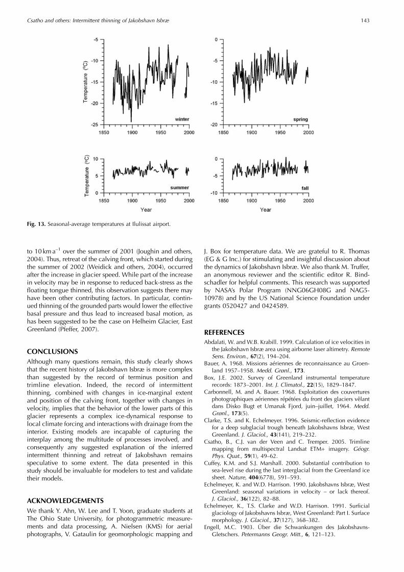
Several periods of distinctly different behavior of thelower reach of Jakobshavn Isbræ can be identified since thepost-LIA maximum stand in 1902. Initially, during the firsthalf of the 20th century, thinning rates were modest. Higherthinning rates, reaching 5–11ma–1, detected during theperiods 1902–13 and 1930–59 are probably associated withregional warming trends. Between 1910 and 1930, averagewinter and spring temperatures increased rapidly (0.58Ca–1;Fig. 13). Although the precise timing of onset of thinning is

somewhat ambiguous, it seems reasonable to attribute theearly period of terminal thinning of Jakobshavn Isbræ tolocal warming.

Continued thinning caused the calving front to becomeungrounded sometime in the late 1940s. The associatedrelease of resistance to flow may have resulted in enhancedcreep rates and thinning of the adjacent grounded portion ofthe glacier lasting until the mid-1980s, although at aprogressively decreasing rate. Between 1953 and 1997 thenorth and south tributaries and the land-based ice sheetaround them exhibited markedly different behavior. Thin-ning of the north tributary continued until 1985 (e.g. Fig. 6)during a period when the calving front was stationary, withonly minor annual fluctuations. Over the south tributary,thinning subsided in the 1960s. North of the fjord, aerialphotographs and satellite imagery indicated continuousretreat of the ice margin until the present, while in the souththe initial retreat was followed by a readvance in the 1960s.

Repeat airborne laser-altimetry surveys indicate that forthe brief period 1993–97 the glacier thickened by severalmeters (Thomas and others, 1995). Our results suggest thatthickening of the northern tributary may have started as earlyas 1985, and near the calving front the average thickeningreached 25ma–1. Thickening rates on the south tributarywere modest and by 1997 the 20–25m elevation differencebetween the tributaries, observed in the mid-1980s byEchelmeyer and others (1991), had disappeared. Thomasand others (1995) argue that this thickening does notrepresent a trend, as it is likely to reflect interannualvariability in surface accumulation and ablation. In particu-lar, the very cold summer of 1992 may have contributedsignificantly to this brief period of thickening. Joughin andothers (2004) note that this interval of thickening corres-ponds to slowing of the glacier between 1985 and 1992,followed by near-constant speeds until 1997. The period ofthickening was short-lived, and �1997 the glacier startedthinning and has continued to do so at increasing rates.

It is tempting to speculate about the causes for this erraticbehavior of thinning and thickening. It may be that, assuggested by Weidick (1968, p.45), the ice margin respondswith a delay of a few years to two decades to fluctuations inclimate. The results discussed in this study suggest that theresponse of Jakobshavn Isbræ to climate forcings involvedcomplex ice dynamics as well.

As pointed out earlier, the calving front becameungrounded in the late 1940s. The release of basal dragresulted in a significant decrease in back pressure on thegrounded portion of the glacier, leading to increasedlongitudinal stretching and consequent glacier thinning.While thinning of the north tributary occurred subsequent tothe ungrounding of the terminus, the rate of inland thinninggradually decreased to zero in the mid-1980s. This scenariocontradicts the instability mechanism proposed by Hughes(1986, 1998), according to which the initial perturbationshould be self-sustained and amplified. Whether furtherthinning and possible glacier collapse was averted by localcooling trends (albeit rather modest (Box, 2002; Fig. 13)) orby adjustment of drainage from the interior to the perturb-ation at the terminus, remains unresolved.

A second observation of interest concerns the recentcollapse of the floating terminus and increase in glacierspeed. Measurements of glacier speed indicate an accelera-tion in flow from an average of 5.7 kma–1 in May 1997 to9.4 kma–1 in October 2000, followed by a further increase

Fig. 12. Retreat of ice-sheet margin from the LIA around Nuna-tarsuaq, north of Kangia Isfjord. Ice-sheet boundaries, measuredfrom aerial photographs, are shown on Landsat ETM+ satelliteimagery acquired on 7 July 2001.


to 10 kma–1 over the summer of 2001 (Joughin and others,2004). Thus, retreat of the calving front, which started duringthe summer of 2002 (Weidick and others, 2004), occurredafter the increase in glacier speed. While part of the increasein velocity may be in response to reduced back-stress as thefloating tongue thinned, this observation suggests there mayhave been other contributing factors. In particular, contin-ued thinning of the grounded parts would lower the effectivebasal pressure and thus lead to increased basal motion, ashas been suggested to be the case on Helheim Glacier, EastGreenland (Pfeffer, 2007).

CONCLUSIONSAlthough many questions remain, this study clearly showsthat the recent history of Jakobshavn Isbræ is more complexthan suggested by the record of terminus position andtrimline elevation. Indeed, the record of intermittentthinning, combined with changes in ice-marginal extentand position of the calving front, together with changes invelocity, implies that the behavior of the lower parts of thisglacier represents a complex ice-dynamical response tolocal climate forcing and interactions with drainage from theinterior. Existing models are incapable of capturing theinterplay among the multitude of processes involved, andconsequently any suggested explanation of the inferredintermittent thinning and retreat of Jakobshavn remainsspeculative to some extent. The data presented in thisstudy should be invaluable for modelers to test and validatetheir models.

ACKNOWLEDGEMENTSWe thank Y. Ahn, W. Lee and T. Yoon, graduate students atThe Ohio State University, for photogrammetric measure-ments and data processing, A. Nielsen (KMS) for aerialphotographs, V. Gataulin for geomorphologic mapping and

J. Box for temperature data. We are grateful to R. Thomas(EG & G Inc.) for stimulating and insightful discussion aboutthe dynamics of Jakobshavn Isbræ. We also thank M. Truffer,an anonymous reviewer and the scientific editor R. Bind-schadler for helpful comments. This research was supportedby NASA’s Polar Program (NNG06GH08G and NAG5-10978) and by the US National Science Foundation undergrants 0520427 and 0424589.

REFERENCESAbdalati, W. and W.B. Krabill. 1999. Calculation of ice velocities in

the Jakobshavn Isbræ area using airborne laser altimetry. RemoteSens. Environ., 67(2), 194–204.

Bauer, A. 1968. Missions aeriennes de reconnaissance au Groen-land 1957–1958. Medd. Grønl., 173.

Box, J.E. 2002. Survey of Greenland instrumental temperaturerecords: 1873–2001. Int. J. Climatol., 22(15), 1829–1847.

Carbonnell, M. and A. Bauer. 1968. Exploitation des couverturesphotographiques aeriennes repetees du front des glaciers velantdans Disko Bugt et Umanak Fjord, juin–juillet, 1964. Medd.Grønl., 173(5).

Clarke, T.S. and K. Echelmeyer. 1996. Seismic-reflection evidencefor a deep subglacial trough beneath Jakobshavns Isbræ, WestGreenland. J. Glaciol., 43(141), 219–232.

Csatho, B., C.J. van der Veen and C. Tremper. 2005. Trimlinemapping from multispectral Landsat ETM+ imagery. Geogr.Phys. Quat., 59(1), 49–62.

Cuffey, K.M. and S.J. Marshall. 2000. Substantial contribution tosea-level rise during the last interglacial from the Greenland icesheet. Nature, 404(6778), 591–593.

Echelmeyer, K. and W.D. Harrison. 1990. Jakobshavns Isbræ, WestGreenland: seasonal variations in velocity – or lack thereof.J. Glaciol., 36(122), 82–88.

Echelmeyer, K., T.S. Clarke and W.D. Harrison. 1991. Surficialglaciology of Jakobshavns Isbræ, West Greenland: Part I. Surfacemorphology. J. Glaciol., 37(127), 368–382.

Engell, M.C. 1903. Uber die Schwankungen des Jakobshavns-Gletschers. Petermanns Geogr. Mitt., 6, 121–123.

Fig. 13. Seasonal-average temperatures at Ilulissat airport.


Engell, M.C. 1904. Undersøgelser og Opmaalinger ved JakobshavnIsfjord og i Orpigsuit i Sommeren 1902. Medd. Grønl., 26(1).

Fastook, J.L., H.H. Brecher and T.J. Hughes. 1995. Derived bedrockelevations, strain rates and stresses from measured surfaceelevations and velocities: Jakobshavns Isbræ, Greenland.J. Glaciol., 41(137), 161–173.

Forman, S.L., L. Marın, C. van der Veen, C. Tremper and B. Csatho.2007. Little Ice Age and neoglacial landforms at the Inland Icemargin, Isunguata Sermia, Kangerlussuaq, west Greenland.Boreas, 36(4), 341–351.

Georgi, J. 1930. Im Faltboot zum Jakobshavner Eisstrom. InWegener, A., ed. Mit Motorboot and Schlitten in Grønland.Bielefeld, Verlag von Velhagen, 157–178.

Georgi, J. 1959. Der Ruckgang des Jakobshavns Isbræ (West-Grønland 698N). Medd. Grønl., 158(5), 51–70.

Hammer, R.R.J. 1883. Undersøgelser ved Jakobshavn Isfjord ognærmeste Omegn i Vinteren 1879–1880. Medd. Grønl., 4(1).

Hughes, T. 1986. The Jakobshavns effect. Geophys. Res. Lett., 13(1),46–48.

Hughes, T.J. 1998. Ice sheets. New York, etc., Oxford UniversityPress.

Johnson, J.V., P.R. Prescott and T.J. Hughes. 2004. Ice dynamicspreceding catastrophic disintegration of the floating part ofJakobshavn Isbræ. J. Glaciol., 50(171), 492–504.

Joughin, I. 2006. Greenland rumbles louder as glaciers accelerate.Nature, 311(5768), 1719–1720.

Joughin, I., W. Abdalati and M.A. Fahnestock. 2004. Largefluctuations in speed of Jakobshavn Isbræ, Greenland. Nature,432(7017), 608–610.

Koch, I.P. and A. Wegener. 1930. Wissenschaftliche Ergebnisse derdanischen Expedition nach Dronning Louises-Land und queruber das Inlandeis von Nordgronland 1912–13. Medd.Grønl., 75.

Long, A.J. and D.H. Roberts. 2003. Late Weichselian deglacialhistory of Disko Bugt, West Greenland, and the dynamics of theJakobshavns Isbrae ice stream. Boreas, 32(1), 208–226.

Luckman, A. and T. Murray. 2005. Seasonal variations in velocitybefore retreat of Jacobshavn Isbrae, Greenland. Geophys. Res.Lett., 32(8), L08501. (10.1029/2005GL022519.)

Mikkelsen, N. and T. Ingerslev, 2002. Nomination of the IlulissatIcefjord for inclusion in the World Heritage List. Copenhagen,Danmarks og Grønlands Geologiske Undersøgelse.

Nordenskiold, A.E. 1871. Redogorelse for 1870 ars expedition tilGronland. Stockholm, Norstedt. Ofversigt Kungliga VetenskabsAkademiens Forhandlingar 1870, 10.973-11.082.

Parizek, B.R. and R.B. Alley. 2004. Implications of increasedGreenland surface melt under global-warming scenarios: ice-sheet simulations. Quat. Sci. Rev., 23(9–10), 1013–1027.

Pfeffer, W.T. 2007. A simple mechanism for irreversible tidewaterglacier retreat. J. Geophys. Res., 112(F3), F03S25. (10.1029/2006JF000590.)

Rignot, E. and P. Kanagaratnam. 2006. Changes in the velocitystructure of the Greenland Ice Sheet. Science, 311(5673),986–990.

Rink, H. 1857. Grønland, geografisk og statistisk beskrevet. Vol. 1:Det nordre Inspektorat. Copenhagen, A.F. Host.

Sohn, H.G., K.C. Jezek and C.J. van der Veen. 1998. JakobshavnGlacier, West Greenland: thirty years of spaceborne obser-vations. Geophys. Res. Lett., 25(14), 2699–2702.

Ten Brink, N.W. 1975. Holocene history of the Greenland ice sheetbased on radiocarbon-dated moraines in West Greenland. Bull.Grønl. Geol. Undersøgelse, 113.

Thomas, R. 2004. Force-perturbation analysis of recent thinningand acceleration of Jakobshavn Isbræ, Greenland. J. Glaciol.,50(168), 57–66.

Thomas, R., W. Krabill, E. Frederick and K. Jezek. 1995. Thickeningof Jacobshavns Isbræ, West Greenland, measured by airbornelaser altimetry. Ann. Glaciol., 21, 259–262.

Thomas, R.H. and 8 others. 2000. Substantial thinning of amajor eastGreenland outlet glacier. Geophys. Res. Lett., 27(9), 1291–1294.

Thomas, R.H., W. Abdalati, E. Frederick, W.B. Krabill, S. Manizadeand K. Steffen. 2003. Investigation of surface melting anddynamic thinning on Jakobshavn Isbræ, Greenland. J. Glaciol.,49(165), 231–239.

Truffer, M., J. Amundson, M. Fahnestock and R.J. Motyka. 2006.High time resolution velocity measurements on JakobshavnIsbræ. [Abstract C11A-1132.] Eos, 87(52), Fall Meet. Suppl.

Van der Veen, C.J. 2001. Greenland ice sheet response to externalforcing. J. Geophys. Res., 106(D24), 34,047–34,058.

Van der Veen, C.J. and B.M. Csatho. 2005. Spectral characteristicsof Greenland lichens. Geogr. Phys. Quat., 59(1), 63–73.

Weidick, A. 1968. Observations on some Holocene glacierfluctuations in West Greenland. Bull. Grønl. Geol. Unders., 73.

Weidick, A. 1969. Investigations of the Holocene deposits aroundJakobshavn Isbrae, West Greenland. In Pewe, T.L., ed. Theperiglacial environment: past and present. Montreal, McGill–Queens University Press, 249–262.

Weidick, A. 1984. Studies of glacier behaviour and glacier massbalance in Greenland: a review. Geogr. Ann., Ser. A, 66(3),183–195.

Weidick, A. 1991. Present-day expansion of the southern part of theinland ice. Rapp. Grønl. Geol. Unders., 152, 73–79.

Weidick, A. 1992. Jakobshavn Isbræ area during the climaticoptimum. Rapp. Grønl. Geol. Unders., 155, 67–72.

Weidick, A. 1995. Greenland. InWilliams, R.S. and J. Ferrigno, eds.Satellite image atlas of glaciers of the world. US Geol. Surv. Prof.Pap. 1386-C, C1–C105.

Weidick,A.,H.Oerter,N.Reeh,H.H. ThomsenandL. Thoring. 1990.The recession of inland ice margin during the Holocene climaticoptimum on the Jacobshavn Isfjord area of west Greenland.Palaeogeogr., Palaeoclimatol., Palaeoecol., 82(3–4), 389–399.

Weidick, A., N. Mikkelsen, C. Mayer and S. Podlech. 2003.Jakobshavn Isbræ, West Greenland: the 2002–2003 collapseand nomination for the UNESCO World Heritage List. Geol.Surv. Den. Greenland Bull., 4, 85–88.

Zwally, H.J., W. Abdalati, T. Herring, K. Larson, J. Saba andK. Steffen. 2002. Surface melt-induced acceleration of Green-land ice-sheet flow. Science, 297(5579), 218–222.

MS received 9 July 2007 and accepted in revised form 5 October 2007


intermittent thinning of jakobshavn isbræ, west greenland ... · intermittent thinning of...

Documents