interbank interest rates and the risk premium · interbank interest rates and the risk premium by...

BIS WORKING PAPERS

No. 81 – November 1999

INTERBANK INTEREST RATES

AND THE RISK PREMIUM

by

Henri Pagès

BANK FOR INTERNATIONAL SETTLEMENTSMonetary and Economic Department

Basel, Switzerland

BIS Working Papers are written by members of the Monetary and Economic Department of the Bank forInternational Settlements, and from time to time by other economists, and are published by the Bank. The papersare on subjects of topical interest and are technical in character. The views expressed in them are those of theirauthors and not necessarily the views of the BIS.

Copies of publications are available from:

Bank for International SettlementsInformation, Press & Library ServicesCH-4002 Basel, Switzerland

Fax: +41 61 / 280 91 00 and +41 61 / 280 81 00

This publication is available on the BIS website (www.bis.org).

© Bank for International Settlements 1999.All rights reserved. Brief excerpts may be reproduced or translated provided the source is stated.

ISSN 1020-0959

BIS WORKING PAPERS

No. 81 – November 1999

INTERBANK INTEREST RATES

AND THE RISK PREMIUM

byHenri Pagès *

Abstract

The paper presents a one-factor affine model of the term structure of Libor rateswith autocorrelated measurement errors. It can be viewed as a central tendencymodel, with the theoretical arbitrage-free rates serving as stochastic means towhich the observed rates revert. Two estimation techniques are compared, onebased on a no-measurement-error assumption, the other on Kalman filtering. Theestimates are then used in standard yield spread regressions with a view toaccounting for the departure of future short rates from what the expectationshypothesis would predict.

* Email: [email protected]. I thank B Cohen, E Remolona, S Gerlach and participants at an internal seminal for valuablecomments and suggestions. Research assistance by M Radjabou is gratefully acknowledged. The views expressed are theauthor’s and not necessarily those of the Bank for International Settlements.

Contents

1. Introduction . . . . . . . . . . . . . . . . . . . . . . . . . . . . . . . . . . . . . . . . . . . . . . . . . . . . . . . . . . . . . . . . . . . . . . 1

2. Some theory . . . . . . . . . . . . . . . . . . . . . . . . . . . . . . . . . . . . . . . . . . . . . . . . . . . . . . . . . . . . . . . . . . . . . . 4

3. Econometric results . . . . . . . . . . . . . . . . . . . . . . . . . . . . . . . . . . . . . . . . . . . . . . . . . . . . . . . . . . . . . .11

3.1 Data and summary statistics . . . . . . . . . . . . . . . . . . . . . . . . . . . . . . . . . . . . . . . . . . . . . . . . .11

3.2 Estimation . . . . . . . . . . . . . . . . . . . . . . . . . . . . . . . . . . . . . . . . . . . . . . . . . . . . . . . . . . . . . . . . .14

4. Analysis of speci�cation biases . . . . . . . . . . . . . . . . . . . . . . . . . . . . . . . . . . . . . . . . . . . . . . . . . . . .19

5. Implications for the expectations hypothesis . . . . . . . . . . . . . . . . . . . . . . . . . . . . . . . . . . . . . . . . .21

5.1 A simple forward rate regression . . . . . . . . . . . . . . . . . . . . . . . . . . . . . . . . . . . . . . . . . . . . .21

5.2 Yield spread regressions . . . . . . . . . . . . . . . . . . . . . . . . . . . . . . . . . . . . . . . . . . . . . . . . . . . . .24

6. Conclusion . . . . . . . . . . . . . . . . . . . . . . . . . . . . . . . . . . . . . . . . . . . . . . . . . . . . . . . . . . . . . . . . . . . . . .26

Appendix A . . . . . . . . . . . . . . . . . . . . . . . . . . . . . . . . . . . . . . . . . . . . . . . . . . . . . . . . . . . . . . . . . . . . . . . . . . .28

Appendix B . . . . . . . . . . . . . . . . . . . . . . . . . . . . . . . . . . . . . . . . . . . . . . . . . . . . . . . . . . . . . . . . . . . . . . . . . . .30

References . . . . . . . . . . . . . . . . . . . . . . . . . . . . . . . . . . . . . . . . . . . . . . . . . . . . . . . . . . . . . . . . . . . . . . . . . . . .32

1. Introduction

Understanding the dynamics of Libor is important for the management of risk. Managers rely heavily

on over-the-counter markets and organised exchanges to hedge or take positions in derivative contracts

whose reference rates are linked to Libor, and this requires a consistent theory of how the market forms

expectations of Eurodeposit rates.

From a monetary policy perspective, considering Libor rates instead of those derived from domestic

government securities can also provide valuable insights into the market’s expectations of future short

rates. The Libor curve may be regarded as an approximation to the true cost of funds for prime

banks participating in the London market. There are no reserve requirements or deposit insurance

premiums imposed on Eurocurrency deposits, no withholding taxes levied on interests paid to non-

resident depositors and, in terms of capital adequacy, no speci�c capital requirements for foreign banks.1

An additional feature of the Libor market is that it provides quotes every day for a wide range of short-

run maturities. By contrast, it is less easy to de�ne the near end of the term structure with government

securities. Short-term instruments used to complement bonds with a horizon of less than one year are not

available for every maturity, and the determination of their rates is often affected by speci�c institutional

features. Finally, the short-term nature of the market, together with its concentration in highly rated

banks subject to strict credit monitoring, implies that the credit premium included in Libor �xings is

probably small. This is not to say that the credit standing of any prime institution cannot deteriorate

rapidly and eventually be re�ected in higher rates. The British Banker’s Association, however, polls a

sample of top-rated banks, trims the highest and lowest rates, rounds the remaining yields and �nally

averages them. As a result, the in�uence of idiosyncratic credit risk in of�cial quotes is likely to be

signi�cantly dampened.

This paper estimates an interbank term structure from a panel of weekly dollar Libor �xings for six

maturities, ranging from one to 12 months. There are two key features. First, the estimation is based

on an equilibrium model of the term structure. Market participants and central banks tend to “read” the

term structure as if it revealed the market’s expectations of future short-term rates. Forward spreads,

however, are driven by changes in the price of risk as well as changes in expectations about interest

rates. Rather than treating excess returns on long bonds as residuals, the equilibrium approach seeks to

elicit term premia endogenously from the absence of arbitrage. Second, it is assumed that expectations

� Europlacements enjoy the same favored risk rating (20%) as the paper issued by federal agencies and supranationalinstitutions, but the situation might change in the wake of the draft proposals for the Basel apital Accord.

1

about future rates can be captured by a single factor. The justi�cation for this choice is to limit

the number of parameters needed to reproduce the Libor curve and avoid computationally intensive

formulations. Instead of increasing the number of factors to describe the entire yield curve, the paper

keeps a single latent variable to �t a smaller part of the yield curve. To some extent, it tries to �nd

a middle ground between the complicated dynamic general equilibrium models of the term structure

developed in the �nancial literature and the simpler static curve-�tting techniques that many (central)

banks use to approximate implied forward rates or their distributions from observed �nancial prices.

The continuous-time, square root model of Cox et al. (1985) has a few remarkable properties. First,

it is tractable, and thus has the potential to be more widely used in central banks as an indicator of

interest rate risk. The factor summarises the current shape of the yield curve and the way it is expected

to �uctuate over time. Second, it allows for a variable term premium, and thus provides a theoretical

decomposition of forward rates into expectations and risk premiums directly. One subject of obvious

interest in this respect is its bearing on the rejection of the expectations hypothesis. Since the largest

discrepancies arise for postwar US data at maturities under two years, it is particularly interesting to

address this issue with Eurodollar data. Finally, the continuous-time formulation avoids the restrictive

assumption of log-normal interest rate innovations at discrete time intervals, which is at odds with the

evidence of a substantial excess kurtosis. In particular, it allows more �exibility in that it can easily

generate a hump-shaped curve for the impact of shocks on the term structure.

The econometric estimation of the model is carried out using two alternative techniques. Following

Chen and Scott (1993) and many others, the �rst one is based on the true conditional density of the

underlying factor, but assumes that there is no measurement error on the six-month Libor. Because the

non-central chi-square density of the factor involves a modi�ed Bessel function, we call it the “Bessel”

method. The second uses a Kalman �lter to let the data determine the measurement errors, but does not

use the true conditional density of the underlying factor. We call this the “Kalman” method. In either

case the measurement errors are assumed to follow simple autoregressive processes, with innovations

that are independent of the factors, normally distributed and possibly cross-correlated. One motivation

for this assumption is that the cross-section averaging and rounding-off of Libor quotes induce serial

correlation in the data. More plausibly, it deals with the risk of misspeci�cation in the model, which can

have a lasting effect on measurement errors. Although we will continue to refer to them as measurement

errors, they can also be interpreted as speci�cation errors.

Our results are as follows. First, we �nd that the one-factor model yields plausible parameter estimates

with a reasonably small measurement error. Interestingly, it can be viewed as a central tendency model,

with the theoretical arbitrage-free rates serving as stochastic means to which the observed rates revert.

2

The bottom line is that the factor is much more persistent than the error term, and this is suf�cient to

explain the main features of the interest rate data. The model has in fact two incarnations, depending

on the econometric method used to estimate it. Both reproduce the various unconditional moments

but the Bessel variant is better at capturing the time-varying shapes of the yield curve and the term

structure of volatility. Second, we show how both econometric methods induce systematic biases, which

lead to Bessel overpredicting and Kalman underpredicting future changes in rates. To this extent, the

speci�cation biases appear to arise less from the model than from the method used to estimate it. Finally,

we show on the basis of standard yield spread regressions that the one-factor model accounts well for

the departure of future short rates from what the expectations hypothesis would predict at the one-year

maturity, although signi�cant tensions remain between the model and the data at the three-month and

six-month maturities.

Recent option pricing literature has placed greater emphasis on interbank interest rates. Jegadeesh

and Pennacchi (1996) estimate a two-factor model with central tendency calibrated on the three-month

Eurodollar futures contracts traded on the Chicago Mercantile Exchange. They show that more than one

factor is required to �t the interest rate dynamics, but their evidence is based on the Vasicek model, which

cannot account for time-varying term premia. Moreno and Peña (1996) explore a single-factor model

with jumps for the Spanish overnight interest rate. They show that the existence of jumps can explain

the systematic underpricing of some interest rate derivatives, but they do not use panel data. Jamshidian

(1997) studies the existence of multifactor arbitrage-free models with a view to pricing Libor and swap

derivatives jointly. The no-arbitrage paradigm can be questioned if, as argued by Duf�e and Singleton

(1997), Libor yields have distinctive features that are not shared by the longer end of the swap yield

curve, for example as a result of heterogeneity in credit quality.

In monetary economics, interbank interest rates have also been studied for their informational or

predictive content. Gerlach and Smets (1997) use Euromarket data for 17 currencies and show that

rejection of the expectations hypothesis is for many countries less cogent than the empirical literature

based on US data would suggest. Malz (1998) �ts zero coupon curves on Eurodeposits, FRAs and swap

rates at different points in time using the popular Nelson-Siegel-Svensson methodology, and argues that

interbank rates are a valuable source of information on market expectations and the stance of monetary

policy. Konstantinov (1998) derives an equilibrium model of the interbank term structure by assuming

that the federal funds target rate is subject to discrete jumps and is able to replicate the predictability

pattern of interest rates for part of the sample.

To better identify the place of this paper in the literature of af�ne-yield models characterised by Duf�e

and Kan (1996), it may be useful to discuss the relative merits of one-factor and multifactor models.

3

Much criticism has been levelled against the one-factor formulation. One main objection is that it

assumes that all information is captured by a single expectation process. Fleming and Remolona (1999),

for example, show that different types of announcements lead to fundamentally different reactions of

the yield curve according to the way market expectations are revised. As an amalgam, a single factor

is also more dif�cult to interpret in terms of outside factors, such as money growth rates, in�ation or

other factors connected to monetary policy. The empirical weaknesses of one-factor models have also

been clearly documented. The main problems concern the shape of the mean yield curve, the changing

patterns of autocorrelations and volatility with maturity, and the fact that interest rate innovations have

substantial excess kurtosis. In addition to these shortcomings, Backus et al. (1998) show that the one-

factor model is incapable of accounting for the departure from the expectations hypothesis and still

maintaining an upward-sloping forward curve. Not surprisingly, all these dif�culties have pointed toward

a larger number of factors, and it seems that nothing can stop authors in their quest for more complicated

models.

At the same time, introducing more factors is no panacea. Ideally, one would like to increase

their number until the discrepancy between observed and modeled rates could be ascribed to a pure

measurement error. In practice, however, the error comes both from the underlying data and the model.

Statistical tests of the overidentifying restrictions, in the rare cases where they fail to reject, can reinforce

con�dence in the model, but it is doubtful that any equilibrium model, however re�ned, will decisively

identify the deep structural parameters that underlie the absence of arbitrage, if there are any. The pitfall

is that by imposing a theoretical straitjacket on the data one may end up modelling the error term. Of

course, adding more factors results in a better �t of the yield curve at any point in time, but this does not

necessarily lead to an improvement in the reliability of the model’s predictions.

This paper is organised as follows. Section 2 summarises some results from the one-factor af�ne-yield

model and its implications for the properties of rates. Section 3 outlines the statistical properties of Libor

and reports the results of our estimations according to the two econometric methods referred to above.

Section 4 provides a brief account of the speci�cation biases generated by those methods. Section 5

presents estimates of standard yield spread regressions, involving ex post returns on rolling over a one-

month investment over different periods, and compares the results with the same regressions obtained

when the dependent variables are generated by the model. Section 6 concludes.

2. Some theory

In �nance theory, the pricing kernel approach highlights the interaction between probabilities and risk.

The paper follows that approach by focusing on the one-factor continuous-time af�ne formulation.

4

Writing the model in continuous time avoids the assumption of log-normal conditional distributions, but

requires that the implied density recorded at discrete intervals be evaluated exactly. Since the derivations

are now standard, this section brie�y recalls the basic formulas and shows how they can be embedded in

an econometric model as the central tendencies to which the observable interest rates revert.

The principle of arbitrage by dynamic trading states that the current price �|cA of a zero-coupon bond

maturing at time � is determined by �|�|cA � E ��A � �|�, where �| is the state price process (or

pricing kernel). The process �| is de�ned as

�| � ��

�� |

f

�r ��

��|(1)

and captures both the effect of pure discounting, where �| is the instantaneous interest rate, and the

market’s valuation of risk, encapsulated in the risk-neutral density �|. One way to arrive at a tractable

speci�cation of movements in the yield curve is to characterise state prices in terms of a few latent state

variables. The paper uses a single-factor representation obeying the square root process

��| � � � �|� ��

�| ��|(2)

where � is a standard Brownian motion, the mean reversion parameter and the steady-state mean.2

The � process models the arrival of information, possibly embodying expectational factors related to

monetary policy or other economic news in some “reduced form” fashion.

With only one factor, it remains to determine how � impacts the price system � and the short-term

interest rate �. It seems reasonable to assume that, in a risk-averse world, positive shocks to the short-

term interest rate (higher �) should be associated with greater anxiety about future rates (higher state

price �), thus inducing a positive correlation between � and � . Suppose, for example, that shocks to

the risk-neutral density �| are proportional to the factor’s innovations:��|�|

� � �

�| ��|

where parameterises the price of risk. With lower-case letters standing for logarithms, Ito’s formula

applied to (1) implies that state prices are ruled by the stochastic differential equation

��| � �| �� 2��| ��

�| ��|�

This formulation makes clear that � governs the covariance between shocks to the price system

(via �|) and shocks to the interest rate (via �|). One would then expect to be negative to induce a

positive correlation between � and � .

Given this setup, a simple Markovian structure obtains when the instantaneous interest rate depends on

the current state. As shown by Duf�e and Kan (1996), the choice �� f� leads to an af�ne term

2 When �� , the process �| never reaches 0. This condition is always met for the parameter values estimated in thesequel.

5

structure. A succinct derivation can be found in Appendix A. The parameter � controls for the lower

bound on the short rate, while �f scales its conditional volatility. Letting � � � � � denote the current

maturity, the bond price �|cA becomes the discount function

�� (3)

for the functions �� and �� given in Appendix A. We call � �� the impact curve. The corresponding

spot rates are

�� (4)

where � �� , or factor loading, expresses the sensitivity of the interest rate to information arrival. The

one-factor af�ne model differs from the standard CIR formulation in that �| � �� |� satis�es

��| � ��Wf � �|� ��

�f �� |

where �Wf � �� f. That is, � may be different from zero, and the entire yield curve is bounded

below by �. (A negative � would imply that rates can become negative with positive probability.)

The cross-sectional and time series behavior of yields under the one-factor model is entirely subsumed

in the �ve-dimensional parameter vector �� f� � ��. This has strong implications. First, all rates are

linear functions of the same factor and, in the absence of measurement errors, are perfectly correlated. In

particular, they are stationary and revert to their respective long-term means at the same rate . Second,

the yield curve tends to a limit which is independent of time as the maturity lengthens. This is illustrated

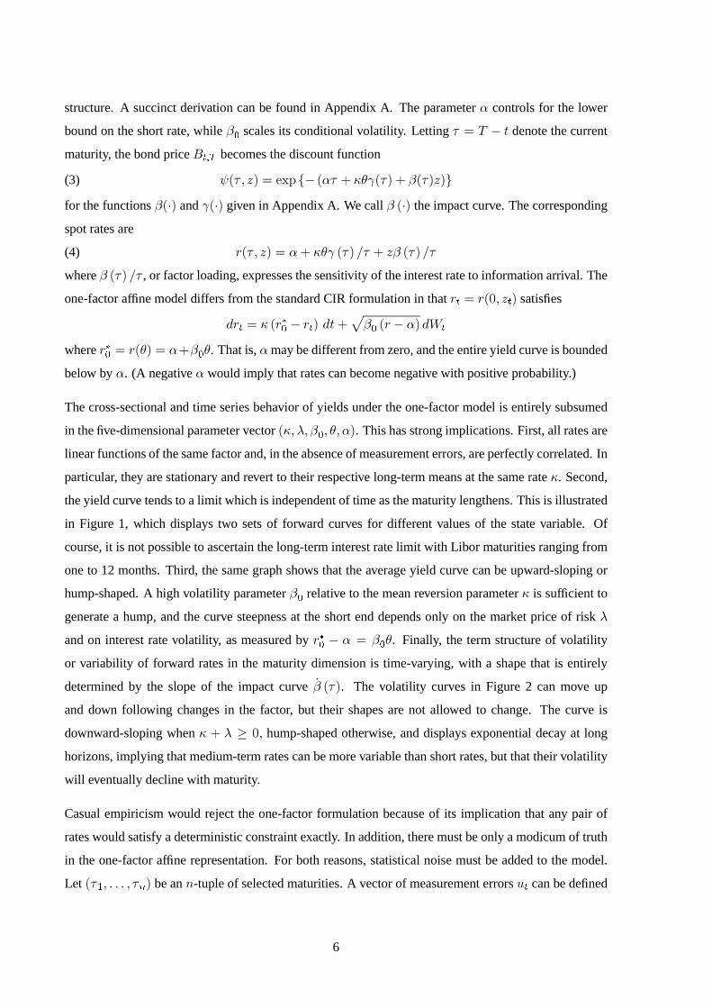
in Figure 1, which displays two sets of forward curves for different values of the state variable. Of

course, it is not possible to ascertain the long-term interest rate limit with Libor maturities ranging from

one to 12 months. Third, the same graph shows that the average yield curve can be upward-sloping or

hump-shaped. A high volatility parameter �f relative to the mean reversion parameter is suf�cient to

generate a hump, and the curve steepness at the short end depends only on the market price of risk

and on interest rate volatility, as measured by �Wf � � � �f. Finally, the term structure of volatility

or variability of forward rates in the maturity dimension is time-varying, with a shape that is entirely

determined by the slope of the impact curve �� . The volatility curves in Figure 2 can move up

and down following changes in the factor, but their shapes are not allowed to change. The curve is

downward-sloping when � �� hump-shaped otherwise, and displays exponential decay at long

horizons, implying that medium-term rates can be more variable than short rates, but that their volatility

will eventually decline with maturity.

Casual empiricism would reject the one-factor formulation because of its implication that any pair of

rates would satisfy a deterministic constraint exactly. In addition, there must be only a modicum of truth

in the one-factor af�ne representation. For both reasons, statistical noise must be added to the model.

Let �� ?� be an �-tuple of selected maturities. A vector of measurement errors �| can be de�ned

6

Figure 1: Forward curve

7

Figure 2: Volatility curve ��

8

from

�&| � ��|� �&� �&| � � � , � � � , ��(5)

where ��|� �&� � �& �& �|�

From (4), the coef�cients are �& � � � ��&� ��& and �& � � ��&� ��&. The continuous-time

dynamic (2) gives rise to the difference equation

�| � � � �� |3� �|(6)

where � � �3V*D2 is the autocorrelation of the factor (alternatively, � � is the weekly rate of mean

reversion). The innovation to the factor, �|, has a conditional distribution which is determined by the

transition function of the state variable � sampled every week. One can show that this conditional

distribution is a non-central chi-square with � degrees of freedom, the analytic form of which

is given in Appendix B. As a result, the unconditional distribution of �| is non-normal3 with variance

�2� � � � �2� �. Measurement errors are assumed to be AR(1) processes,

�&| � �&�&|3� &| � E �| � �(7)

with innovations that are independent of the factors, normally distributed and possibly cross-correlated.

In general, �| is not observable, and (5) can be viewed as the measurement equation of a �ltering problem

with transition equation (6) and error covariance structure (7).

With the general AR(1) formulation provided by (6) and (7), the signal extraction problem in (5) might

seem unidenti�ed at �rst sight. Indeed, if the �rst component were itself a generic AR(1) process, it

would be dif�cult to disentangle the factor from the error term, and the factor loadings �& would not

be identi�ed. However ��|� �&� is a vector process whose mean, covariance and autocorrelation are

determined by an arbitrage model. Consider the following thought experiment. First, �-difference the

data suitably at all maturities until the error terms become serially uncorrelated. This determines the �&s.

Second, use the covariance matrix of the observed rates to estimate the covariance of the innovation

error �. With six maturities, there remain six �rst-moment conditions to estimate the twelve coef�cients

�&, �& and the parameters �, and �2� in (6). But all these coef�cients are determined by a model based

on the �ve-dimensional parameter �� f� � ��. Hence, the model is actually slightly overidenti�ed.

Finally, to draw the link between (5–7) and a model where one factor reverts to a time-varying mean, we

select any maturity � and write (5) in �rst difference using (6) and (7) to obtain

��&| � � � ��W& � �&|3�

� �� &�

��&��|3�� &|3�

� &| �& �|(8)

where we have put �&��|� � ��&� �|� and �W& � �&�� to simplify notation. In addition to the �xed

long-run mean �W&, to which the interest rate �&| reverts at rate � �, we recover the standard central

� It is actually a gamma distribution (see Appendix B1).

9

tendency formulation where the time-varying rate �&��|� plays the role of the target driving the future

path of the interest rate, with rate of mean reversion �� &. Conversely, the central tendency model

�!| � � � ��|3� � !|3�� |

�| � � � ��W � |3�� |

where the factor !| reverts to a time-varying factor | can be reinterpreted in terms of the econometric

model

!| � | �|

�| � ��|3� �|

with �| � |��|� � � ��W�|3��. When � is close to one, the error term � is hardly distinguishable

from a pure error innovation, and it may be that the �rst factor is simply the central tendency itself up

to some AR(1) process. To this extent, an investigator requiring that all rates be linear functions of both

! and may in fact be unduly imposing arbitrage constraints on the autocorrelated error term �|. By

contrast, in (5) all arbitrage constraints are captured in �&��|�, not in the error term.

The introduction states that the one-factor formulation can easily generate hump-shaped responses to

the arrival of new information. In the central tendency model, the hump comes from the interaction

between two factors. When surprise information is revealed to the central tendency, the �rst factor

starts adjusting towards its new target, but its movements are limited by the size of � �. During the

adjustment period, the central tendency, which is itself mean-reverting, gradually declines toward its

steady-state value, lowering the �rst factor’s initial deviation from target. The impact of the innovation

is therefore felt more sharply for intermediate maturities than for short and long ones. By contrast,

multifactor Vasicek (1977) models with homoskedastic volatility, such as in Longstaff and Schwartz

(1992) or Chen and Scott (1993), imply constant term premia and cannot generate a hump. However,

time-varying conditional variances can also accommodate a hump-shape in the one-factor model.4 A

necessary and suf�cient condition for the factor loading curve to be upward-sloping at inception is that

the price of risk associated with holding debt be larger in absolute value than the mean reversion

parameter . This implies that the initial rise in the term premium more than offsets the speed at which

the short rate is expected to return to an equilibrium. The relationship between risk and expectational

factors is further examined in Section 5.1.

e This is shown in Appendix A, where our model is taken as the limit of a sequence of heteroskedastic discrete-timemodels.

10

3. Econometric results

Our �rst approach follows Chen and Scott (1993). We assume that one of the rates� the often referenced

six-month Libor � is observed without error. This actually sidesteps the identi�cation problem by

making �| an observable variable. The estimation then proceeds using maximum likelihood under the

conditional factor transition and the joint distribution of measurement errors. Because the true density

involves a modi�ed Bessel function, it is referred to in the sequel as the “Bessel” estimation. The second

approach is based on the Kalman �lter. This quasi-maximum likelihood procedure exploits the �rst two

moments of the conditional density of observed yields. We depart from the standard application of the

Kalman �lter in taking the model’s arbitrage conditions as well as the serial correlation of measurement

errors into account. Details of the two estimations are given in Appendix B.

While each approach is relatively easy to implement, they both lead to inconsistent estimates. The

no-measurement-error assumption allows direct observation of the underlying factor, but the resulting

distribution of yields cannot be taken as a correct description of the data generating process. In

particular, the variance of the underlying factor is equated to that of the six-month Libor, even though

the latter should be larger in the presence of uncorrelated measurement errors. We thus predict that the

unconditional variance of the factor, �, will be biased upwards. On the other hand, the Kalman �lter

lets the data determine the measurement errors for all yields, but uses normality assumptions that are

not met by a non-Gaussian model. The estimated factor can still be interpreted as an optimal predictor

in the mean squared error sense, rather than in the conditional mean sense, but the parameter estimates

do not minimise the conditional density of the data generating process. These biases are examined in

Section 4.

3.1 Data and summary statistics

We obtain end-of-week Libor of�cial �xing data from Reuters as reported in the DRI database for 24

October 1986 to 20 February 1998 for maturities ranging from one to 12 months (592 observations).

The selected maturities are one, two, three, six, nine and 12 months. Each bank in the panel is asked

to contribute the rate at which it could borrow funds, were it to do so by asking for and then accepting

interbank offers in reasonable market size, just prior to 11.00 a.m. Eurodeposit rates are volatile but,

due to the trimming, rounding-off and averaging operations, of�cial quotes are not. Table 1 shows the

occurrence of identical consecutive entries in Libor �xing data for various maturities. Repetitions are

indeed quite common from one week to the next, especially for one-month rates.

Some properties of Eurodollar yields are summarised in Table 2. One feature is the shape of the average

yield curve, which is displayed in Figure 3. Some more perspective has been provided to the average

11

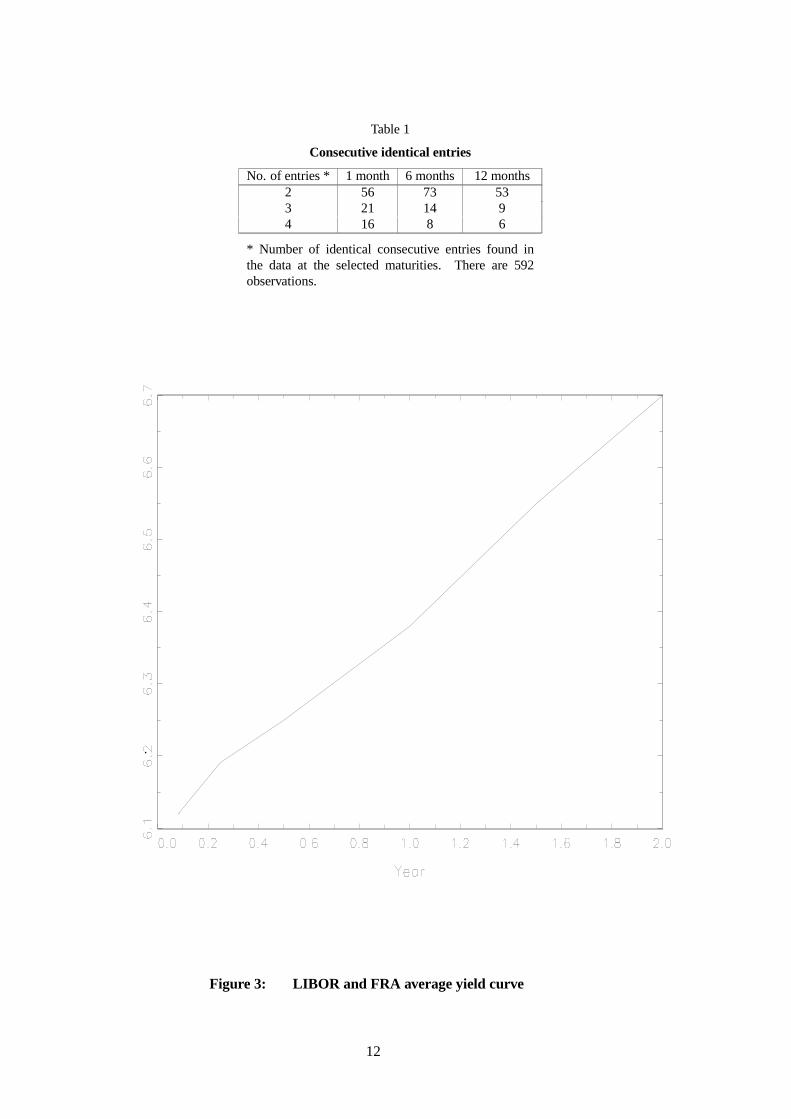
Table 1

Consecutive identical entries

No. of entries * 1 month 6 months 12 months2 56 73 533 21 14 94 16 8 6

* Number of identical consecutive entries found inthe data at the selected maturities. There are 592observations.

Figure 3: LIBOR and FRA average yield curve

12

Table 2

Descriptive statistics of observed and estimated Libor

Average of Libor yields/spreads�n � � ��

Sample �4��n � �4 ��

Bessel ��4��n � ��4 ��

Kalman ��4��n � ��4 ��

Standard deviation of Libor

�n 1.860 1.841 1.828 1.781 1.739 1.697Sample �n � �4 — 0.130 0.177 0.287 0.385 0.464

��n 0.174 0.133 0.141 0.148 0.162 0.159

��n 1.840 1.827 1.816 1.774 1.735 1.692Bessel ��n � ��4 — 0.103 0.141 0.234 0.309 0.393

��n 0.161 0.132 0.141 0.147 0.155 0.155

��n 1.766 1.775 1.781 1.783 1.760 1.715Kalman ��n � ��4 — 0.008 0.015 0.017 0.006 0.050

��n 0.143 0.143 0.144 0.144 0.142 0.139

First autocorrelation of Libor

�n 0.996 0.997 0.997 0.996 0.996 0.995Sample �n � �4 — 0.65 0.78 0.89 0.92 0.94

��n - 0.02 - 0.04 0.04 0.05 - 0.01 0.03

��n 0.996 0.997 0.997 0.996 0.996 0.996Bessel ��n � ��4 — 0.63 0.78 0.89 0.92 0.94

��n - �� - �� 0.05 0.05 0.02 0.04

��n 0.997 0.998 0.998 0.998 0.997 0.996Kalman ��n � ��4 — 0.63 0.77 0.89 0.92 0.94

��n 0.10 0.13 0.19 0.37 0.24 0.14Skewness/kurtosis of weekly changes in Libor

Sample ��n - �� - � � �� - �� - �� - �� - �� 2Bessel ��n - �� - �� - �� - �� - �� - ��Kalman ��n - �� - �� - �� - �� - � � �� - ��

The data are end-of-week 11 a.m. �xing rates as calculated by the British Bankers’ Association. The sample periodis from 24 October 1986 to 20 February 1998 (592 observations). �n is the continuously compounded annual yield,�n � �4 the spread relative to the one-month rate and ��n is the weekly change in yields. Estimated rates arepredicated on equation (8). Bessel means estimation with no measurement error on the six-month LIBOR, Kalmanmeans estimation using a Kalman �lter. The parameter values are � ��, � ��, �

3� ��, � ��,

� � �� for the former and � �� , � ��, �3 � ��, � ��, � � �� for the latter.

13

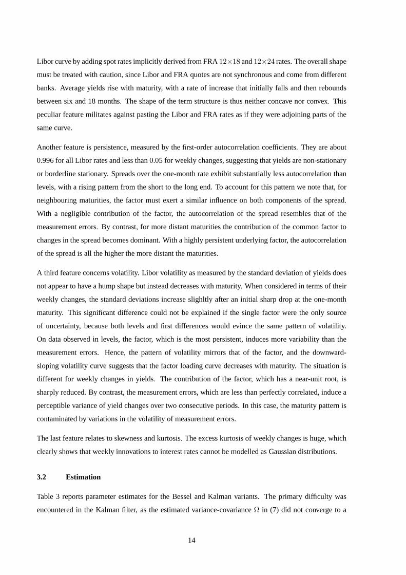
Libor curve by adding spot rates implicitly derived from FRA � and � rates. The overall shape

must be treated with caution, since Libor and FRA quotes are not synchronous and come from different

banks. Average yields rise with maturity, with a rate of increase that initially falls and then rebounds

between six and 18 months. The shape of the term structure is thus neither concave nor convex. This

peculiar feature militates against pasting the Libor and FRA rates as if they were adjoining parts of the

same curve.

Another feature is persistence, measured by the �rst-order autocorrelation coef�cients. They are about

0.996 for all Libor rates and less than 0.05 for weekly changes, suggesting that yields are non-stationary

or borderline stationary. Spreads over the one-month rate exhibit substantially less autocorrelation than

levels, with a rising pattern from the short to the long end. To account for this pattern we note that, for

neighbouring maturities, the factor must exert a similar in�uence on both components of the spread.

With a negligible contribution of the factor, the autocorrelation of the spread resembles that of the

measurement errors. By contrast, for more distant maturities the contribution of the common factor to

changes in the spread becomes dominant. With a highly persistent underlying factor, the autocorrelation

of the spread is all the higher the more distant the maturities.

A third feature concerns volatility. Libor volatility as measured by the standard deviation of yields does

not appear to have a hump shape but instead decreases with maturity. When considered in terms of their

weekly changes, the standard deviations increase slighltly after an initial sharp drop at the one-month

maturity. This signi�cant difference could not be explained if the single factor were the only source

of uncertainty, because both levels and �rst differences would evince the same pattern of volatility.

On data observed in levels, the factor, which is the most persistent, induces more variability than the

measurement errors. Hence, the pattern of volatility mirrors that of the factor, and the downward-

sloping volatility curve suggests that the factor loading curve decreases with maturity. The situation is

different for weekly changes in yields. The contribution of the factor, which has a near-unit root, is

sharply reduced. By contrast, the measurement errors, which are less than perfectly correlated, induce a

perceptible variance of yield changes over two consecutive periods. In this case, the maturity pattern is

contaminated by variations in the volatility of measurement errors.

The last feature relates to skewness and kurtosis. The excess kurtosis of weekly changes is huge, which

clearly shows that weekly innovations to interest rates cannot be modelled as Gaussian distributions.

3.2 Estimation

Table 3 reports parameter estimates for the Bessel and Kalman variants. The primary dif�culty was

encountered in the Kalman �lter, as the estimated variance-covariance � in (7) did not converge to a

14

Table 3

Af�ne-yield model estimates

Bessel Kalman

� � ��

0.24 0.07 3.4 0.31 0.08 3.8 - �� 0.06 - �� - �� 0.13 - ��3 0.25 0.03 10.0 0.66 0.16 4.2 16.2 4.7 3.4 2.4 1.2 2.0� 1.8 0.3 6.1 5.5 0.9 6.4�4 0.81 0.02 43 0.82 0.02 46�5

0.85 0.02 55 0.86 0.01 59�6 0.85 0.02 54 0.86 0.01 58�7 — — — 0.72 0.06 11�8

0.74 0.02 28 0.75 0.03 28�9 0.87 0.02 54 0.88 0.01 59

Mean log likelihood 13.9 13.8

The parameters , , �3, and � refer to the mean reversion rate, price of risk, short rate volatility, long-

run mean of the factor and lower bound on yields, respectively. The parameters �n are the autocorrelationcoef�cients of measurement errors at maturities of one, two, three, six, nine and 12 months. The concentratedcovariance matrix of the Bessel log-likelihood function (no measurement error) is used in the Kalman �lter.The standard errors and t-statistics of parameter estimates are based on the usual Hessian matrix.

positive-de�nite matrix. The Bessel estimation does not have that problem since the variance-covariance

matrix of residuals is actually concentrated out of the likelihood function. For simplicity, we have

equated the Kalman variance of residuals with the Bessel one, interpolating the six-month variance from

those of the neighbouring maturities and setting all remaining cross-variances to zero in the estimation.

This restriction is admittedly arbitrary, but re�ects our prior that, if the biases implied by both methods

are not too severe, the covariance structure of the innovations to �tting errors should be relatively

close. The Kalman parameter estimates are not sensitive to the particular value chosen for the unknown

variance at the six-month maturity within its prescribed range.

The estimates are of the correct sign and magnitude. They are statistically signi�cant, although the

small-sample properties of our Libor data do not vindicate the use of asymptotic theory. They differ

signi�cantly across the two approaches, but remain broadly consistent with the features of the data

highlighted in the previous subsection. The mean reversion parameter is lower for the Bessel than

for the Kalman estimation. The estimated values are 0.24 and 0.32 respectively, which corresponds

to half-lives of 2.9 and 2.2 years. As argued before, the no-measurement-error assumption makes the

factor look more volatile than it actually is. This higher variance is supported by a lower , since a low

mean reversion leads to a more volatile factor. The two mean reversion estimates are associated with

autocorrelation coef�cients of 0.995 and 0.994 (weekly), slightly less than the sample autocorrelations

of yields at various maturities, which are about 0.996. Thus, the common factor absorbs most of the high

15

persistence in yields, leaving measurement errors with substantially less autocorrelation. This difference

in persistence between the factor and the measurement errors was a key feature needed to explain the

contrasted patterns of volatility and persistence observed in Libor data. The estimated autocorrelation

coef�cients of the errors, between 0.7 and 0.9, are quite comparable across the two estimations, but this

may be a consequence of the common covariance assumption mentioned above.

The identifying restriction used to disentangle the factor and the measurement errors is the absence of

arbitrage, which places cross-section restrictions on the coef�cients of the measurement equation (5).

If a second factor has been left out of the analysis, these restrictions will be violated, since the single

factor will not capture all the restrictions implied by arbitrage. A test of the overidentifying restrictions

should thus bear out the model on the number of factors. We estimate the model, under both approaches,

with no restriction placed on (5) and carry out standard likelihood ratio tests, keeping the autocorrelation

parameters and the covariance of measurement errors constant. The likelihood ratio statistic (twice the

change in sample likelihood), which is "2 with 12 degrees of freedom, is 27.0 for Bessel and 13.8 for

Kalman. The corresponding signi�cance levels are 1% and 30%. The test thus favors the latter approach

while rejecting the former, but the result must be treated with care since, among other caveats, it should

be noted that the Kalman likelihood is not the true density of the underlying model.

It is interesting to contrast the performance of the two methods, since their parameter estimates imply

very different shapes for the theoretical forward and volatility curves. Figure 4 compares the mean

theoretical curves �� with the actual mean curve. Average Libor increases by about two basis

points each month beyond the two-month maturity, and this quasi-linear relation makes it dif�cult to

�t a model which generates a hump-shaped term structure. Statistical information about the �tting

errors �&| � �&| � ��&� �|� is reported in Table 4. The model curves approximate the average curve to

within a few basis points.5 Except for the one-month maturity, the standard deviations of the Bessel

innovations are about half the bid/ask spread of 12.5 basis points during the sample period. By contrast,

the estimated standard deviations of the Kalman innovations are about three times as large. In this

respect, the former method fares better than the latter. However, the autocorrelations of �tting errors, �,

are in both cases different from the estimates �� taken from Table 3. It turns out that the Bessel (Kalman)

method systematically underestimates (overestimates) the autocorrelations of �tting errors, suggesting

D Because the slow rates of mean reversion imply that the long-run mean � is not estimated with precision, the populationmean �� of the factor is different from the estimated value ��. One �nds �� for Bessel and �� forKalman, while the estimates of the long-run means are �� and �� . The unconditional variance of �� can beapproximated as ��2� , where � is the length of the period (in years). The corresponding standard errors are 4.9% and1.4%. We calibrate � and the shift parameter � to minimize the discrepancy between the theoretical and the mean yieldcurves, leaving unchanged the three parameters �, and

f, which determine the shape of the forward and volatility

curves.

16

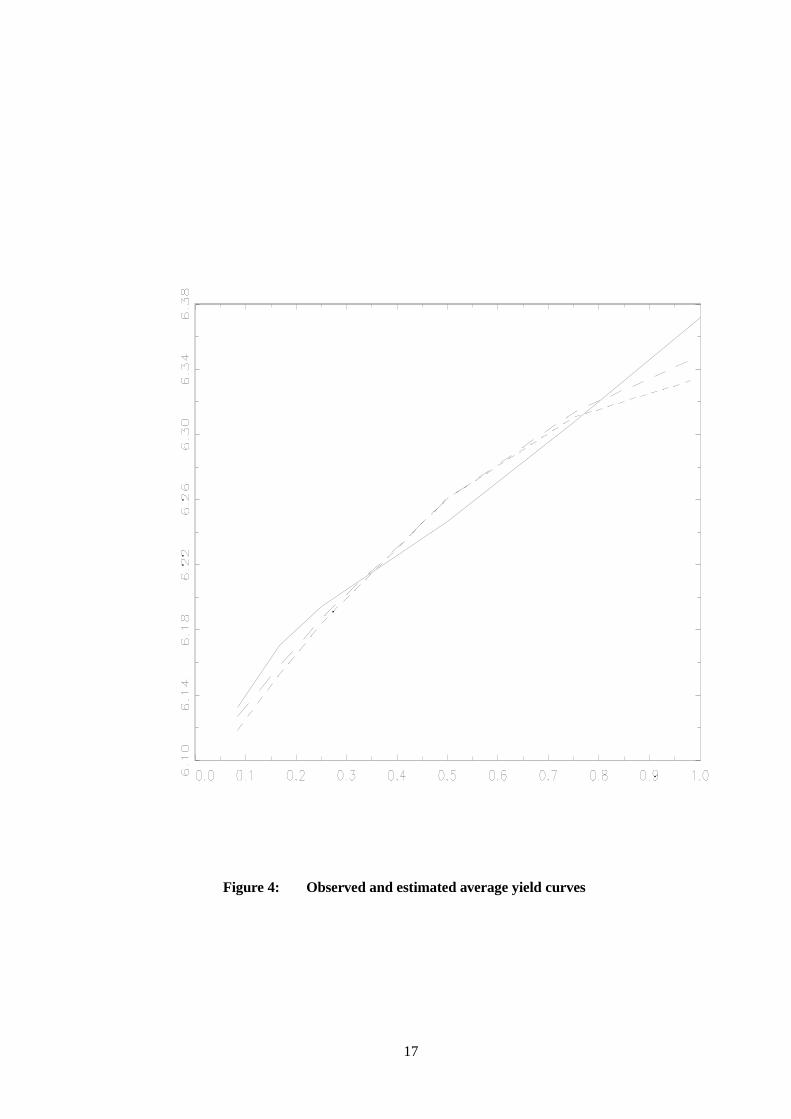
Figure 4: Observed and estimated average yield curves

17

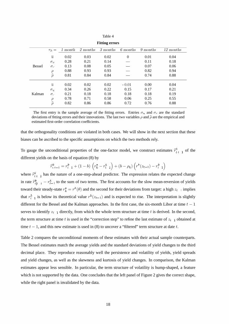
Table 4

Fitting errors

�n � � ��

� 0.02 0.03 0.02 0 0.01 0.04�x 0.28 0.21 0.14 — 0.11 0.18

Bessel �� 0.13 0.08 0.05 — 0.07 0.06� 0.88 0.93 0.93 — 0.82 0.94�� 0.81 0.84 0.84 — 0.74 0.88

� 0.02 0.02 0.02 - �� 0.00 0.04�x 0.34 0.26 0.22 0.15 0.17 0.21

Kalman �� 0.21 0.18 0.18 0.18 0.18 0.19� 0.78 0.71 0.58 0.06 0.25 0.55�� 0.82 0.86 0.86 0.72 0.76 0.88

The �rst entry is the sample average of the �tting errors. Entries �x and �� are the standarddeviations of �tting errors and their innovations. The last two variables � and �� are the empirical andestimated �rst-order correlation coef�cients.

that the orthogonality conditions are violated in both cases. We will show in the next section that these

biases can be ascribed to the speci�c assumptions on which the two methods rely.

To gauge the unconditional properties of the one-factor model, we construct estimates ��&|�|3�

of the

different yields on the basis of equation (8) by

��&|�|3� � �&|3� � � ��W& � �&|3�

� �� &�

��&��|3�� &|3�

�where ��&

|�|3�has the nature of a one-step-ahead predictor. The expression relates the expected change

in rate ��&|�|3�

� �&|3� to the sum of two terms. The �rst accounts for the slow mean-reversion of yields

toward their steady-state �W& � �&�� and the second for their deviations from target: a high �|3� implies

that �&|3� is below its theoretical value �&��|3�� and is expected to rise. The interpretation is slightly

different for the Bessel and the Kalman approaches. In the �rst case, the six-month Libor at time � �

serves to identify �|3� directly, from which the whole term structure at time � is derived. In the second,

the term structure at time � is used in the “correction step” to re�ne the last estimate of �|3� obtained at

time �� , and this new estimate is used in (8) to uncover a “�ltered” term structure at date �.

Table 2 compares the unconditional moments of these estimates with their actual sample counterparts.

The Bessel estimates match the average yields and the standard deviations of yield changes to the third

decimal place. They reproduce reasonably well the persistence and volatility of yields, yield spreads

and yield changes, as well as the skewness and kurtosis of yield changes. In comparison, the Kalman

estimates appear less sensible. In particular, the term structure of volatility is hump-shaped, a feature

which is not supported by the data. One concludes that the left panel of Figure 2 gives the correct shape,

while the right panel is invalidated by the data.

18

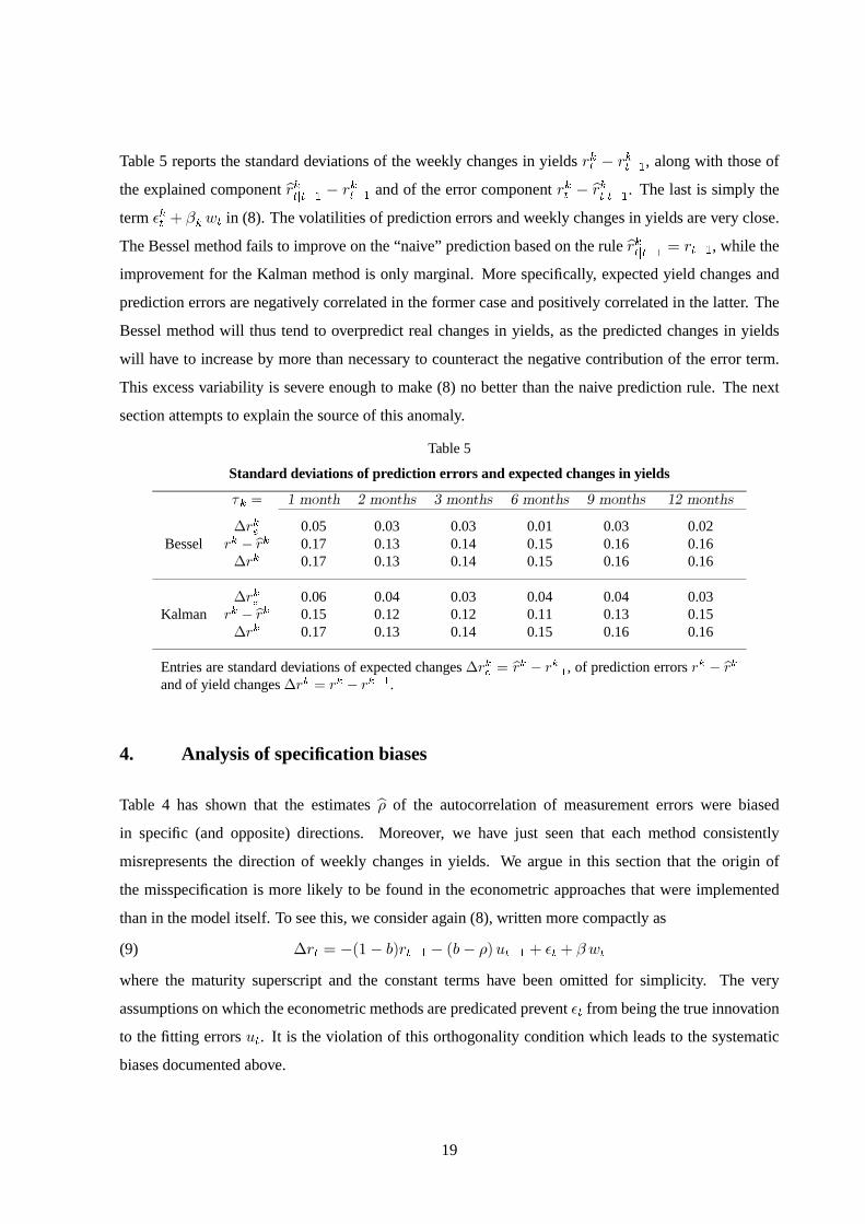
Table 5 reports the standard deviations of the weekly changes in yields �&| � �&|3�, along with those of

the explained component ��&|�|3�

� �&|3� and of the error component �&| � ��&|�|3�

. The last is simply the

term &| �& �| in (8). The volatilities of prediction errors and weekly changes in yields are very close.

The Bessel method fails to improve on the “naive” prediction based on the rule ��&|�|3�

� �|3�, while the

improvement for the Kalman method is only marginal. More speci�cally, expected yield changes and

prediction errors are negatively correlated in the former case and positively correlated in the latter. The

Bessel method will thus tend to overpredict real changes in yields, as the predicted changes in yields

will have to increase by more than necessary to counteract the negative contribution of the error term.

This excess variability is severe enough to make (8) no better than the naive prediction rule. The next

section attempts to explain the source of this anomaly.

Table 5

Standard deviations of prediction errors and expected changes in yields

�n � � ��

��nh 0.05 0.03 0.03 0.01 0.03 0.02Bessel �n � ��n 0.17 0.13 0.14 0.15 0.16 0.16

��n 0.17 0.13 0.14 0.15 0.16 0.16

��nh 0.06 0.04 0.03 0.04 0.04 0.03Kalman �n � ��n 0.15 0.12 0.12 0.11 0.13 0.15

��n 0.17 0.13 0.14 0.15 0.16 0.16

Entries are standard deviations of expected changes ��nh � ��n � �n�4

, of prediction errors �n � ��nand of yield changes ��n � �n � �n�4.

4. Analysis of speci�cation biases

Table 4 has shown that the estimates �� of the autocorrelation of measurement errors were biased

in speci�c (and opposite) directions. Moreover, we have just seen that each method consistently

misrepresents the direction of weekly changes in yields. We argue in this section that the origin of

the misspeci�cation is more likely to be found in the econometric approaches that were implemented

than in the model itself. To see this, we consider again (8), written more compactly as

��| � �� |3� � �� |3� | � �|(9)

where the maturity superscript and the constant terms have been omitted for simplicity. The very

assumptions on which the econometric methods are predicated prevent | from being the true innovation

to the �tting errors �|. It is the violation of this orthogonality condition which leads to the systematic

biases documented above.

19

Consider �rst the Bessel approach. Here we assume that there is no error on the six-month Libor,

mistakenly identifying the factor as �� #, where # is the measurement error on the six-month

rate. Substituting �� for � in (9), we �nd that the measurement innovation becomes� | � |��#| � �#|3��.

Thus, cov �� |� �|3�� cov �� #�, where �� is the autocorrelation of the omitted six-month

error. In general, the sign of the correlation will depend on the relative persistence and covariances

of measurement errors. However, the pattern of autocorrelations in Table 3 strongly suggests that a

minimum is reached at the six-month maturity. Assuming positive comovements between measurement

errors, this implies cov �� |� �|3�� $ �. Table 6 con�rms that all correlations are indeed positive and

signi�cant, pointing to a clear violation of the orthogonality conditions. This has two implications.

First, noting that the model de�nes measurement errors as � | � �| � ��|3�, one has

cov �� |� �|3�� cov ��| � ��|3�� |3�� var ��

so that �� % �, as Table 6 reveals. Second, the prediction error and predicted yield changes in (9) tend to

move in opposite directions, as yields are expected to decline when � is high. The Bessel forecast must

overestimate the direction of change.Table 6

Orthogonality conditionsCross-correlation of measurement errors and lagged error term

� � � �� Bessel 0.16 0.23 0.24 — 0.13 0.19

Kalman ��

Consider now the Kalman approach. Here, the error term �|3� � �|3��|3�� is no longer exogenous

and equation (9) can be rewritten as

��| � �� |3� �� |3� | ��|� �| � �| � ��|3��(10)

The Kalman �lter reestimates both �|3� and �| on the basis of new information at time �. A large

interest rate innovation may be due to a large innovation to the factor � in which case �| will be

increased � or to the fact that the state at time � � was underestimated � in which case �|3� will be

increased. If the weighting is applied properly, both �| and �|3� will be revised in a manner that leaves

the resulting measurement error | uncorrelated with �|3�. Unfortunately, the method de�nes �| as the

mean squared error forecast of a variable that has a large kurtosis. As a result, it gives more weight

to �| than necessary, squeezing both | and �|3� in the process. The excessive factor variability thus

generates positive comovements between | and �|3�. Table 6 indicates that the correlation between |

and �|3� � �|3�� |3� is indeed negative. This naturally has the reverse implications for the estimated

autocorrelations of measurement errors (�� $ �) and the direction of change (underprediction).

20

5. Implications for the expectations hypothesis

The one-factor model is the most parsimonious way to generate a risk premium endogenously. It thus

has implications for the predictability of interest rates. In this section, we use the estimations above to

see if the one-factor model is capable of accounting for the evidence against the expectations hypothesis.

The predictability “smile”, i.e. the fact that yield spreads help forecast future short rates at short and

long horizons but less so at horizons of about a year, is a major stumbling block of the expectations

hypothesis.

To understand intuitively how the one-factor model behaves with respect to the expectations hypothesis,

we assume away measurement errors and start with a simple forward rate regression involving the short

rate. We then use a standard form of yield spread regression involving changes in one-month Libor to

examine whether the one-factor model conforms with the predictability pattern of interest rates observed

in the data.

5.1 A simple forward rate regression

The expectations hypothesis has several forms. A typical statement is that forward rates are the

expectations of future short rates, up to a constant term premium

&�| � �| � �E| �|n� � �|� '�(11)

where & �| � �| is the forward spread and E| �|n� � �| is the expected change in the instantaneous rate.

The expectations hypothesis can be tested by estimating the regression

�|n� � �| � ( ��&�| � �|� #|(12)

where #| � �|n� � E| �|n� is the forecast error. If the hypothesis is true, then � � and ( � �'� .

Many explanations for the rejection of the expectations hypothesis have focused on a time-varying term

premium. As is well known, if the residual #| is contaminated by a risk premium, � will deviate from

one due to a standard omitted variable problem.

According to the one-factor model, the theoretical expressions for the expected change in yields and the

risk premium are, respectively,

E| �|n� � �| � �f� � �3V� � � � �|�

'�| &�| � E| �|n� �

�� f� � �3V� �

�� f�

3V��

�|�

To understand intuitively these expressions, consider a positive shock to the expectations process �|,

which shifts the term structure upwards. Expected yields are revised downwards, since mean reversion

implies that the short rate will gradually return to its equilibrium level. On the other hand, the shape of

21

the yield curve is also in�uenced by variations in the term premium.6 When interest rates are expected to

fall, borrowers prefer to pay high short rates until long rates eventually fall. Similarly, investors attempt

to invest in long-term bonds in the hope of locking in high yields. The result of both responses is to raise

the risk premium at the shorter end of the maturity spectrum and reduce it at the longer end, causing the

term premium to be �rst negatively then positively correlated with expected yield changes.

To ascertain � in the context of the one-factor model without measurement error, we consider (11) as a

signal extraction problem, where the term premium varies through time. The implied regression slope

�� f� � �3V� ��f � �� (13)

is displayed in Figure 5. The af�ne model endogenously creates a predictability smile, but it generates

a regression coef�cient that is greater than one for maturities under two years. To this extent, it worsens

the situation by moving the regression coef�cient in the wrong direction. The reason is clear. Over

short-term horizons, a positive shock to the expectations process �| moves the expected change in the

short rate and the term premium in opposite directions. Thus, a falling forward spread indicates that

the expected component has declined even further. In this case, expected changes in the short rate tend

to overpredict the magnitude of forward spreads, making � greater than one. The inability of af�ne

models to generate both a rising mean forward rate curve and a regression slope between zero and one

is well known, see Backus et al. (1998). This is also true in the present continuous-time framework. The

average forward curve is upward-sloping if and only if � �� % �. This implies that the volatility

curve �� cannot fall at a faster rate than . With �� f, this yields �� $ �f�3V� , and the

numerator in (13) is larger than the denominator.

The regression slope equation (13) assumes that all shocks to interest rates are captured by a single

factor. As a result, the expected yield change and the term premium are perfectly correlated. A large

negative correlation raises the regression slope above one. In practice, however, one would expect a

less than perfect correlation. With systematic measurement errors, the one-factor model provides at

best a rough approximation to the true expected yield changes and risk premia. Indeed, part of the

interest rate dynamics has been left unexplained and shifted instead to measurement errors. Thus, even

though in theory the one-factor model cannot account for regression slopes of less than one in a simple

regression such as (12), in practice the presence of systematic measurement errors will bias the slope

estimates downwards. It would be unfortunate to discard the af�ne model just because we require that

S The effect on the risk premium depends on �� f�3V� . Since �� , whether the rate

of change of the impact curve �rst derivative, ��, is above or below �� depends on the sign of � �� . For shortmaturities �� is close to zero so �� is negative and �� must lie above

f�3V� . For long maturities, ��

becomes eventually positive and �� decreases faster than f�3V� . The term premium turns negative as �� cuts

below f�3V� .

22

Figure 5: Predictability pattern implied by the one-factor model

23

it �t all rates exactly, for we would not know if a given shift in the term structure were due to a shift in

expectations or risk premia.

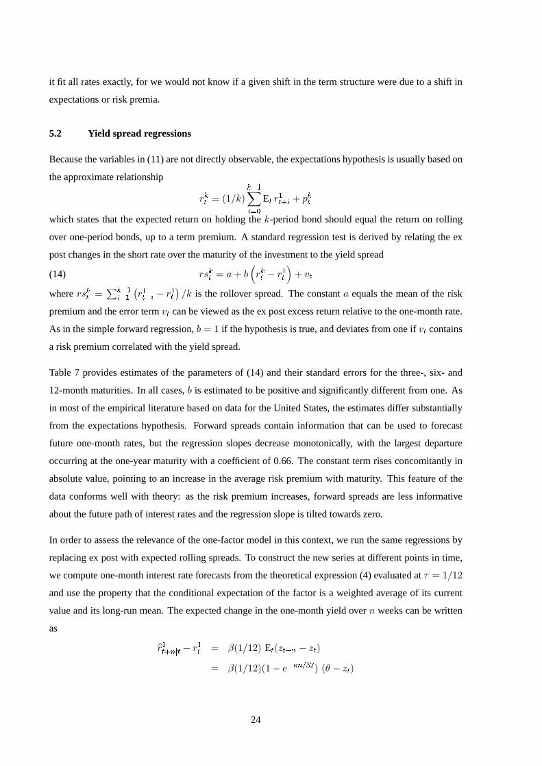
5.2 Yield spread regressions

Because the variables in (11) are not directly observable, the expectations hypothesis is usually based on

the approximate relationship

�&| � � ��&3��'f

E| ��|n� '&|

which states that the expected return on holding the �-period bond should equal the return on rolling

over one-period bonds, up to a term premium. A standard regression test is derived by relating the ex

post changes in the short rate over the maturity of the investment to the yield spread

��&| � ( ��&| � ��|

� #|(14)

where ��&| ��&3�

�'�

��|n� � ��|

�� is the rollover spread. The constant ( equals the mean of the risk

premium and the error term #| can be viewed as the ex post excess return relative to the one-month rate.

As in the simple forward regression, � � if the hypothesis is true, and deviates from one if #| contains

a risk premium correlated with the yield spread.

Table 7 provides estimates of the parameters of (14) and their standard errors for the three-, six- and

12-month maturities. In all cases, � is estimated to be positive and signi�cantly different from one. As

in most of the empirical literature based on data for the United States, the estimates differ substantially

from the expectations hypothesis. Forward spreads contain information that can be used to forecast

future one-month rates, but the regression slopes decrease monotonically, with the largest departure

occurring at the one-year maturity with a coef�cient of 0.66. The constant term rises concomitantly in

absolute value, pointing to an increase in the average risk premium with maturity. This feature of the

data conforms well with theory: as the risk premium increases, forward spreads are less informative

about the future path of interest rates and the regression slope is tilted towards zero.

In order to assess the relevance of the one-factor model in this context, we run the same regressions by

replacing ex post with expected rolling spreads. To construct the new series at different points in time,

we compute one-month interest rate forecasts from the theoretical expression (4) evaluated at � � �

and use the property that the conditional expectation of the factor is a weighted average of its current

value and its long-run mean. The expected change in the one-month yield over � weeks can be written

as

��|n?�| � ��| � �� E|��|n? � �|�

� �� 3V?*D2� � � �|�

24

Table 7

Rollover spread regressions

Yield spread regression Parameter estimates��nw � ( �

��nw � �4w

#w Maturity �( (s.e.) �� (s.e.)

3 months - �� (0.01) 0.77 (0.09)��nw 6 months - �� (0.02) 0.69 (0.07)

12 months - �� (0.03) 0.66 (0.06)

3 months - �� (0.00) 0.98 (0.03)��n>hw 6 months - �� (0.00) 0.87 (0.01)

12 months - �� (0.01) 0.64 (0.01)

The regressions use the Newey and West (1987) correction for MA errors of order �. The dependentvariable is either ��nw , the ex post rollover spread, or ��n>hw , the rollover spread estimated from theBessel model.

where the factor �| is taken from one of the two approaches described above. For space reasons we

discuss only the results obtained for the Bessel estimation.

The coef�cient estimates from the model are presented in Table 7 for comparison. The model is able to

replicate the predictability smile, and the �tted values accord particularly well with the evidence at the

one-year horizon. The estimated mean risk premia also track their sample counterparts closely. The one-

month regression slope estimate, by contrast, is very close to what the expectations hypothesis would

dictate. This may be evidence that the one-factor model imposes an excessive negative correlation

between the rolling spread and the risk premium, or that it underestimates the variability of the risk

premium. To assess whether the rollover spread identi�ed with the model ��e| is a good predictor of the

ex post rollover spread ��|, we also estimate univariate �-step-ahead forecasting equations of the form

��| � ) � ��e| �|�(15)

using various yield spreads as overidentifying restrictions. The results in Table 8 present compelling

evidence that the model 12-month rollover spread is a good predictor of its empirical counterpart, but the

same hypothesis is soundly rejected at the three- and six-month maturities. One plausible interpretation

is that the one-factor model is too parsimonious to capture the behaviour of interest rates in the short

term.The low '-values associated with the tests of overidentifying restrictions indicate that current short-

and long-term rates help improve forecasts, so that the predictions based on (15) are not informationally

ef�cient. In short, the one-factor model provides a good approximation to the behaviour of interest rates

at the horizon of one year and leads to better forecasts than the expectations hypothesis, but there remain

signi�cant tensions between the model and the data at short maturities.

25

Table 8

Forecasting equations of the rollover spread

Forecasting equation Parameter estimates��nw � ) � ��n>hw �w Maturity �) (s.e.) �� (s.e.) '-value

1 month - �� (0.01) 0.45 (0.06) 0.001 overidentifying 3 months - �� (0.01) 0.70 (0.07) 0.01

restriction 12 months - �� (0.03) 0.99 (0.07) 0.45

1 month 0.00 (0.01) 0.42 (0.05) 0.003 overidentifying 3 months - �� (0.01) 0.69 (0.06) 0.01

restrictions 12 months - �� (0.03) 0.96 (0.07) 0.05

The forecasting equations use either one overidentifying restriction (the yield spread with the samehorizon as the rollover spread) or three overidentifying restrictions (all yield spreads). The '-valuesare the marginal probabilities associated with the tests of the overidentifying restrictions.

6. Conclusion

This paper tries to explain movements in Libor rates with a single-factor af�ne-yield model. We �nd

that this model provides a reasonable approximation of the unconditional and conditional properties of

Libor rates, with the Bessel approach providing more sensible parameter estimates than the Kalman

method on the basis of the implied volatility patterns and the size of error innovations. We point out

that it approximates well the behaviour of future rates at the horizon of one year, although signi�cant

tensions remain between the model and the data at shorter maturities. We also argue that the evidence

of misspeci�cation is likely to originate from the implausible assumptions on which the econometric

methods are predicated rather than from the model itself.

A consistent �nding of the term structure literature is that, to reconcile the time-series dynamics of

interest rates with their cross-sectional shapes, models with more than one factor are necessary. We feel

nevertheless that the paper’s effort to con�ne strictly the number of factors needed to explain Libor rates

is justi�ed.

First, the choice of a model should re�ect the application to which it is put. If the objective is to

manage interest rate risk through sophisticated trading strategies, the need to capture all sources of

uncertainty may require a large number of factors. For central banks, however, the situation is different.

They are more interested in extracting markets’ expectations about future interest rates than in pricing

interest rate risk accurately. As latent variables, factors are neither amenable to straightforward economic

interpretation, nor very suggestive of the joint behavior of short- and long-term interest rates. They may

also fail to provide a sensible account of the predictability pattern of interest rates.

26

Second, as emphasised in Gong and Remolona (1997), it is important to know whether separate models,

with a reduced number of factors, can �t small stretches of the yield curve. Explaining only part of

the curve holds some promise that it will become possible to �t the whole curve with an appropriately

speci�ed model. This seems especially true with an interbank term structure including FRA prices and

interest rate swaps, since market players have different creditworthiness. An interest rate swap curve, for

example, could be derived by discounting future Libor �xings at a risk-adjusted rate. A “driving factors”

approach to the joint behaviour of interest and default rates would gather evidence on how banks have

shifted their undiversi�able risks to other institutions, without having to assume that the Libor and swap

markets have homogeneous credit quality. A related example can be found in the pricing of discount

Brady bonds which, with different contractual arrangements, could be used to uncover sovereign credit

risk. Both examples are part of the author’s research agenda.

27

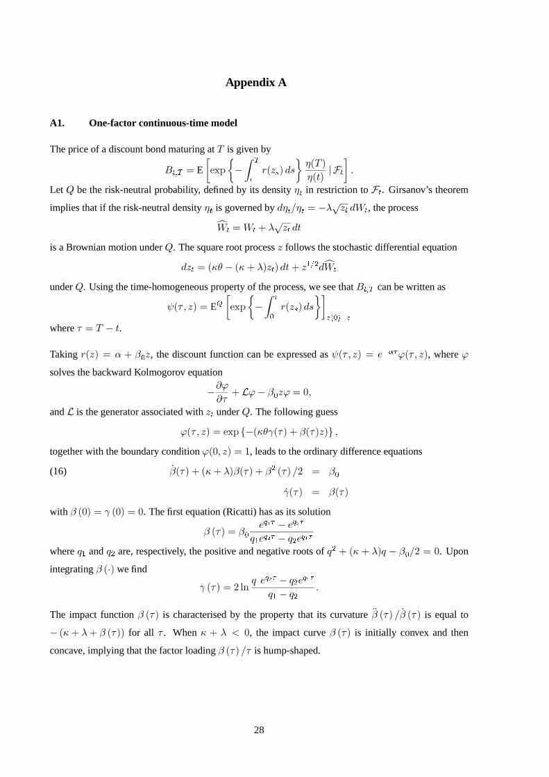
Appendix A

A1. One-factor continuous-time model

The price of a discount bond maturing at � is given by

�|cA � E��

�� A

|

��r� ��

��

�� |

�

Let * be the risk-neutral probability, de�ned by its density �| in restriction to �|. Girsanov’s theorem

implies that if the risk-neutral density �| is governed by ��|��| � � �

�| ��|, the process

��| � �| �

�| ��

is a Brownian motion under *. The square root process � follows the stochastic differential equation

��| � � � � ��|�� *2��|

under *. Using the time-homogeneous property of the process, we see that �|cA can be written as

�� E'

��

��

f

��r��

� 5Ef�'5

where � � � � �.

Taking �� f�, the discount function can be expressed as �� 3k�+�� , where +

solves the backward Kolmogorov equation

�,+

,� �+� �f�+ � ��

and � is the generator associated with �| under *. The following guess

+��

together with the boundary condition +�� , leads to the ordinary difference equations

�� 2 �� f(16)

��

with � �� . The �rst equation (Ricatti) has as its solution

� �� f�^4� � �^5�

-��^5� � -2�^4�

where -� and -2 are, respectively, the positive and negative roots of -2 � �- � �f� � �. Upon

integrating � �� we �nd

� �� -��

^5� � -2�^4�

-� � -2�

The impact function � �� is characterised by the property that its curvature �� is equal to

� � � �� for all � . When % �, the impact curve � �� is initially convex and then

concave, implying that the factor loading � �� is hump-shaped.

28

To study the average yield curve, it is convenient to consider forward rates. Taking the derivative of the

discount function yields

&��

and the mean forward rate curve has a slope given by

�&��

The slope at the origin is positive and equal to �& � � �f � � ��W � ��. It eventually turns negative

if �" � -� $ �, in which case it is hump-shaped. The last condition is met if either 2 % �f

or 2 $ �f and ��

2 � �f��

2 � �f

�.

The volatility term structure can be derived by �xing the maturity date � so that � � � � �. The change

of variable &A| � &�� leads to

�&A| � � �� | ��

�*2| ��|

so that the forward volatility curve is de�ned by �� *2| . Since the rate of increase in �� is

� � � ��, its slope is governed initially by and, for large � , decays at a rate of -�.

A2. Hump shapes in independent factor models

We show that discrete-time af�ne models with independent factors can accommodate hump shapes

provided they account for a time-varying term premium. Consider the recursion that characterises the

factor loadings in a one-dimensional Cox-Ingersoll-Ross model� see for example Backus et al. (1998),

p. 9:

�?n� � 2� �?+� � �?��2�(17)

starting with �f � �. We posit

� ��

�f

+ � �

for some �f, and small $ �. By this token, the difference equation (17) can be seen as an element of

the sequence of recursions indexed by and de�ned by

�"?n� � 2� �"

?� � �� "?

��f �

2��

Let �"? � �f �

"?. We obtain

�"?n� � �"

?

� �f � � ��"

? � �"2? �

where � � �

�f. Thus, �"? converges to the solution to (16) as �. A necessary and suf�cient

condition for a hump is that � % �, a condition equivalent to � + � % �.

29

Appendix B

B1. No-measurement-error assumption (Bessel method)

Let �e be the six-month Libor rate. From (4) and (5) with �e � �, we obtain

�e| � �e �e �|�

The sample loglikelihood at time � can be decomposed into two parts.

�� . With the above change of variable, the �rst part of the log-likelihood is

�� &��|��|3�� e, where &��|��|3�� is the density of �| conditional on �|3� one week before. The

function & can be written as

&��|��|3�� )

�!

.

�D*2

�� ! .�� /D��

!.�

where ) �

� �3V*D2

! � )�|

. � )�3V*D2 �|3�

0 � � $ �

/D�� modi�ed Bessel function of the �rst kind.

For the Bessel function, we have used the integral representation provided by Gradshteyn and Ryzhik

(1980), p. 958. Details about the numerical implementation are available from the author. For the �rst

observation, we used the unconditional distribution of �, which is the gamma function

�� nD

�� 0��D�32V5�

�� . Letting &| � �&| ��&�&|3�, where �| is the vector of �tting errors

for the �ve remaining rates, the second part is

�

�|�

3� | �

��

��1��

The covariance matrix can be concentrated out of the likelihood function, using

� ��A|'2 |

�

|

��

B2. Linear �lter (Kalman method)

We start the Kalman �lter by writing the model (2–5) as

�| � � � �� |3� �|� var��|� � - � � � �2��

�| � � ��| �|

�| � 2�|3� |� var� � � �

30

where � � �3V�and 2 is the diagonal matrix containing the autocorrelation coef�cients of measurement

errors. Using ��| � �| �2�|3�, we can transform the model as

�| � � � �� |3� �|

��| � 34 �|3� | ��|

with 3 � � � �� / � 2�� and 4 � ��/ � 2��. Note that the measurement innovation of the

transformed model is no longer uncorrelated with the factor innovation, and that the state variable at

date � is �|3�.

In the prediction step, we use the rules

�|3��|3� � � � �� |32�|3� �|3��|3�

�|�|3� � �

��|�|3� � 34 �|3��|3��

Let �2|�|3�

be the conditional variance of �|3�. The covariance matrix of the prediction errors is�� 2

|�|3�� 2

|�|3�4 �

� - -��

�2|�|3�

-� �|�|3�

��

where �|�|3� � � -�� 2|�|3�

44 �.

In the correction step, we de�ne 5| ��| �3�4 �|3��|3�

and �nd

�|3��| � �|3��|3� �2|�|3�4��3�

|�|3�5|

�|�| � -��3�|�|3�

5|

the conditional variance of which is

�5c�

|�|�

��2|�|3�

�

� -

��

�2|�|3�

4 �

-��

�|�|3�

��2|�|3�

4 -��

Thus,

�2|n��| ��

� ��5c�

|�|

��

� �2�2|�|3� - �

�-�� 2|�|3�4

�

��3�|�|3�

�-� ��2|�|3�4

�and the Kalman �lter is

�|�| � � � �� |3��|3� 6| 5|

with 6| ��2

|�|3�4 � -��

��3�|�|3�

. To start the �lter, we extract �� from

�� var�� var�� 7

with 7�� .

31

References

Backus D, S Foresi, A Mozumdar and L Wu (1998): “Predictable changes in yields and forward rates”

Working Paper No. 6379, National Bureau of Economic Research, January.

Chen R and L Scott (1993): “Maximum likelihood estimation for a multifactor equilibrium model of the

term structure of interest rates” �� 3, pp. 14–31.

Cox J, J Ingersoll and S Ross (1985): “A theory of the term structure of interest rates” ��

53, pp. 385–407.

Duf�e D and R Kan (1996): “A yield-factor model of interest rates” �� 6, pp. 379–

406.

Duf�e D and K Singleton (1997): “An econometric model of the term structure of interest rate swap

yields” !�� 52(4), pp. 1287–1321.

Fleming M and E Remolona (1999): “The term structure of announcement effects” Working Paper

No. 71, Bank for International Settlements, June.

Gerlach S and F Smets (1997): “The term structure of Euro-rates: some evidence in support of the

expectations hypothesis” �� " �� 16(2), pp. 305–321.

Gong F and E Remolona (1997): “Two factors along the yield curve” � #�� "$

�� % !�� ##��, Blackwell, pp. 1–31.

Gradshteyn I and I Ryzhik (1980): ! �� &� ��$ ��$ �� . Academic Press,

Orlando.

Jamshidian F (1997): “Libor and swap market models and measures” �� 1(4),

pp. 293–330.

Jegadeesh N and G Pennacchi (1996): “The behavior of interest rates implied by the term structure of

Eurodollars futures” �� "$ �� ' �(��& 28(3), pp. 426–446.

Konstantinov V (1999): “Fed funds rate targeting, monetary regimes and the term structure of interbank

rates” Manuscript, Harvard University, January.

Longstaff F and E Schwartz (1992): “Interest rate volatility and the term structure: A two-factor general

equilibrium model” �� , 47, pp. 1259–82.

32

Malz A (1998), “Interbank interest rates as term structure indicators” Research Paper No. 9803, Federal

Reserve Bank of New York, March.

Moreno M and I Peña (1996): “On the term structure of interbank interest rates: Jump-diffusion

processes and option pricing” Discussion Paper No. 24, Universitat Pompeu Fabra.

33

Recent BIS Working Papers

No. Title Author

65April 1999

Higher profits and lower capital prices: is factor allocationoptimal?

P S Andersen, M Klauand E Yndgaard

66April 1999

Evolving international financial markets: someimplications for central banks

William R White

67May 1999

The cyclical sensitivity of seasonality in US employment Spencer Krane andWilliam Wascher

68May 1999

The evolution of determinants of emerging market creditspreads in the 1990s

Steven B Kamin andKarsten von Kleist

69June 1999

Credit channels and consumption in Europe: empiricalevidence

Gabe de Bondt

70June 1999

Interbank exposures: quantifying the risk of contagion Craig H Furfine

71June 1999

The term structure of annoucement effects Michael J Fleming andEli M Remolona

72August 1999

Reserve currency allocation: an alternative methodology SrichanderRamaswamy

73August 1999

The Taylor rule and interest rates in the EMU area: a note Stefan Gerlach andGert Schnabel

74August 1999

The dollar-mark axis Gabriele Galati

75August 1999

A note on the Gordon growth model with nonstationarydividend growth

Henri Pagès

76October 1999

The price of risk at year-end: evidence from interbanklending

Craig H Furfine

77October 1999

Perceived central bank intervention and market expecta-tions: an empirical study of the yen/dollar rate, 1993–96

Gabriele Galati andWilliam Melick

78October 1999

Banking and commerce: a liquidity approach Joseph G Haubrichand João A C Santos

79November 1999

Pass-through of exchange rates and import prices todomestic inflation in some industrialised economies

Jonathan McCarthy

80November 1999

A note on alternative measures of real bond rates Palle Andersen

ISSN 1020-0959

interbank interest rates and the risk premium · interbank interest rates and the risk premium by...

Documents