Intensity Analysis of Spatial Point PatternsGeog 210C

Introduction to Spatial Data Analysis

Chris Funk

Lecture 4

2

Spatial Point Patterns

DefinitionSet of point locations with recorded “events" within study region, e.g., locations of trees, disease or crime incidents

point locations could correspond to all possible events or to subsets of them (mapped versus sampled point pattern)attribute values could have also been measured at event locations, e.g., tree diameter (marked point pattern)

Objective: Introduce statistical tools for quantifying spatial variations in event intensity

3

Some Objectives in Spatial Point Pattern Analysis

Intensity analysis objectivescharacterize patterns of spatial distribution of event locationsdetermine where events are more likely to occur in spaceinvestigate relationships between spatial “clusters" and nearby sources or other factors

NoteThe above should be contrasted with the case of spatially continuous data, where analysis objectives often involve characterizing spatial variation in attribute values recorded at a fixed set of locations/units

4

Outline

Concepts & NotationQuadrat Counts for Intensity Estimation1D Kernel Density Estimation2D Kernel Density EstimationPoints To Remember

5

Some Notation

Point eventsSet of N locations of events occurring in a study area:

Variable of interesty(s) = number of events (a count) within arbitrary domain or support s with measure (length, area, volume) |s|; support s is centered at an arbitrary location u and can also be denoted as s(u); in statistics, y(s) is treated as a realization of a random variable (RV) Y(s)In other words, we are interested in studying the spatial distribution of the count realizations y(s) generated from the respective RVs Y(s)

6

Intensity of Events

Local intensity λ(u)Mean number of events per unit area at an arbitrary location or point u

where E{Y(s)} denotes the expectation (mean) of RV Y(s) defined over a region s(u) centered at u.

Overall intensity λEstimated asWhere where |D| = measure (area) of study region D

Region-specic intensityFor a constant intensity λ(u) = λ the expected number of events within a region s is just a function of |s|i.e., E{Y(s)} = λ|s|;

7

Local Intensity Estimation via Quadrat Counts I

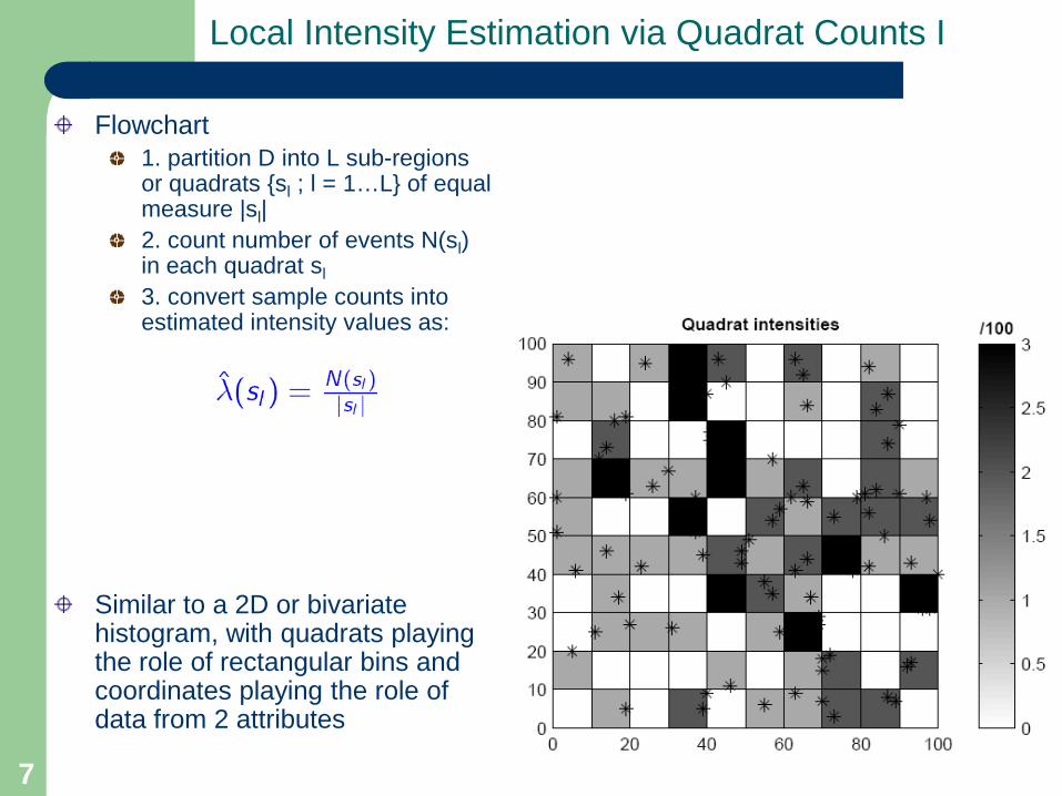
Flowchart1. partition D into L sub-regions or quadrats {sl ; l = 1…L} of equal measure |sl|2. count number of events N(sl) in each quadrat sl3. convert sample counts into estimated intensity values as:

Similar to a 2D or bivariate histogram, with quadrats playing the role of rectangular bins and coordinates playing the role of data from 2 attributes

8

Local Intensity Estimation via Quadrat Counts II

Characteristicsestimated intensities λ(sl) over set of quadratsintended for revealing large-scale patterns in intensity variation over Dlarger quadrats yield smoother intensity maps; smaller quadrats yield “spiky“ intensity maps with empty quadratssliding and overlapping quadrats, as well as randomly placed quadrats, can also be usedsize, origin, and shape of quadrats matters a lot

9

Intensity or Density Estimation in 1D

Consider a hypothetical 1D point pattern comprised of N = 10 events (left) and estimate their local intensity, i.e., a 1D profile of average # of events per unit area:

Statistical analogyThe objective is to describe the density of x-coordinates, and this problem has been treated extensively in the non-parametric density estimation literature; a first-cut at such a density profile is provided by the density histogram plot (right).In other words: the set of N x-coordinates of events in a 1D point pattern can be viewed as N values of an attribute, here the x-coordinate . . .

10

Density Estimation Preview

Key conceptsdensity estimation via a histogram calls for deciding on: (i) the number of attribute classes (bins), and (ii) their centers in the abscissainstead of choosing a limited # of bins, choose as many bins as the # of events in the data setbars in a histogram are rectangular, but nothing prevents us from using other shapes to build a density profile…

Another key concept: Each bar (left) or triangle (right) can be regarded as the influence of an observed event to the likelihood of seeing other events around that observed one …

11

1D or Univariate Kernel I

Kernel functionAnalytical expression for likelihood of a particular x-coordinate, or in other words for probability of observing an event at the particular x-coordinate, given presence of an event at coordinate xi

Kernel characteristics Ifunction of distance hi = |x-xi| between arbitrary point at location x and event at location xi : k(x,xi ) = k(|x-xi|) = ki(h), where h is the distance between an arbitrary location x and the kernel center, here the event location xi (assumed to be at x = 0 on the graph)typically all N kernels are assumed the same, i.e., ki(h) = k(h), for all i

12

1D or Univariate Kernel II

Kernel characteristics II

kernels are (typically symmetric) probability density functions (PDFs), hence non-negative and integrating to 1:

as PDFs, kernels have a mean (0, since the abscissa quanties distance from an event) and positive finite variance:

Relation to density estimationInstead of fixing the # of bins and their origin (as done with histograms) we canestimate the local density f(x) at an arbitrary x-value as a weighted sum of N values k(x-xi); each such value belongs to a different kernel ki(h) centered at a xilocation/coordinate

13

Some 1D Kernel Functions I

rectangular or uniform or Parzen:

triangular:

For a set of P values {xp; p = 1…P} discretizing a 1D segment, and for a particular datum coordinate xi, the function k(xp-xi) can be evaluated P times, and the resulting kernel "profile" can be stored in a (Px1) array ki = [k(xp-xi),p=1…P]T

14

Some 1D Kernel Functions II

Quadratic or Epanechnikov:

Gaussian:

Kernels that reach 0 asymptotically, e.g., Gaussian, are called non-compact kernels

15

Scaled 1D Kernels I

Alternative view of a kernelA kernel function k(x-xi) quantifies the “influence" of a particular event at coordinate xi to its surroundings, i.e., to all other x-locations

Scaling the kernelThe influence of an event at xi to all x-coordinates can be altered by scaling the associated kernel function k(x-xi ); i.e., by dividing the function argument x-xi by a constant b (called the kernel bandwidth); in order to ensure that the new kernel is a PDF, i.e., integrates to 1, divide the output of this new function by b

16

Scaled 1D Kernels II

Scaled kernel functionDivide the argument (distance from event) of the kernel function by a scalar b:

Transformation of PDFsLet X be a RV with PDF fX(x) and Y be another RV defined as Y = (1/b)X, i.e., y = x/b.The PDF fγ(y) of RV Y can be computed as: fγ(y) = (1/b)fX(x/b); if the original PDF fX(x) has std deviation 1, the new PDF fY(y)

has std deviation b

For a set of P values {xp ; p = 1…P} discretizing a 1D segment, and for a particular datum coordinate xi the scaled function k(xp-xi; b) can be evaluated P times, and the resulting discrete kernel stored in a (Px1) array ki(b) = [k(xp-xi;b); p = 1…P]T

17

y Flowchart

1D Kernel Density Estimation Flowchart1. choose a kernel function k(x-xi), i.e., a PDF, and a bandwidth parameter b controlling kernel extent and consequently the “smoothness" of the final estimated density profile f(x); this amounts to choosing a scaled kernel function k(x-xi;b)2. discretize 1D segment, i.e., choose a set of P x-coordinates {xp; p = 1…P} at which the density function f(x) will be estimated3. for each datum coordinate xi , evaluate the scaled kernel function k(xp-xi;b) for all P x-values; this yields N scaled kernel profiles {ki(b); i = 1…N} each one stemming from a particular event coordinate xi4. for each discretization coordinate xp, compute estimated density f(xp) as the sum of the N scaled kernel values k(xp-xi; b), after weighting each such value by 1/N:

OutputA (Px1) vector k(b) with estimated density values f(x) at the specified x-coordinates; the N scaled & weighted kernels {(1/N)ki(b); i = 1…N} can be regarded as N elementary profiles whose super-position builds up the final estimated density profile

18

1D Kernel Density Estimation Examples I

Rules exist for choosing an “optimal" bandwidth parameter, typically based on a pre-supposed distribution type, e.g., Gaussian, for the N data … Estimated density profiles are more sensitive to choice of bandwidth parameter b than to choice of kernel type …

19

1D Kernel Density Estimation Examples II

The smaller the bandwidth, the spikier (noisier) the resulting estimated density profile; too large a bandwidth leads to over-smoothed (with no interesting details) density profiles…

20

Separable 2D Kernels

Two 1D Gaussian kernels

2D composite kernel

SeparabilityAny (scaled or not) 2D kernel that can be derived as a product of 2 elementary1D kernels is called separable

event location ui = (xi;yi), arbitrary location u = (x; y), kernel bandwidths bx and by

bivariate Gaussian PDF for 2 independent RVs, a product of 2 univariate Gaussian PDFs

21

Constructing A Separable 2D Kernel

Two 1D Gaussian kernels for the x- and y-dimensions

Replicated 1D Gaussian kernels and 2D separable composite

Anisotropic kernel = multidimensional kernel with different bandwidths along different directions

22

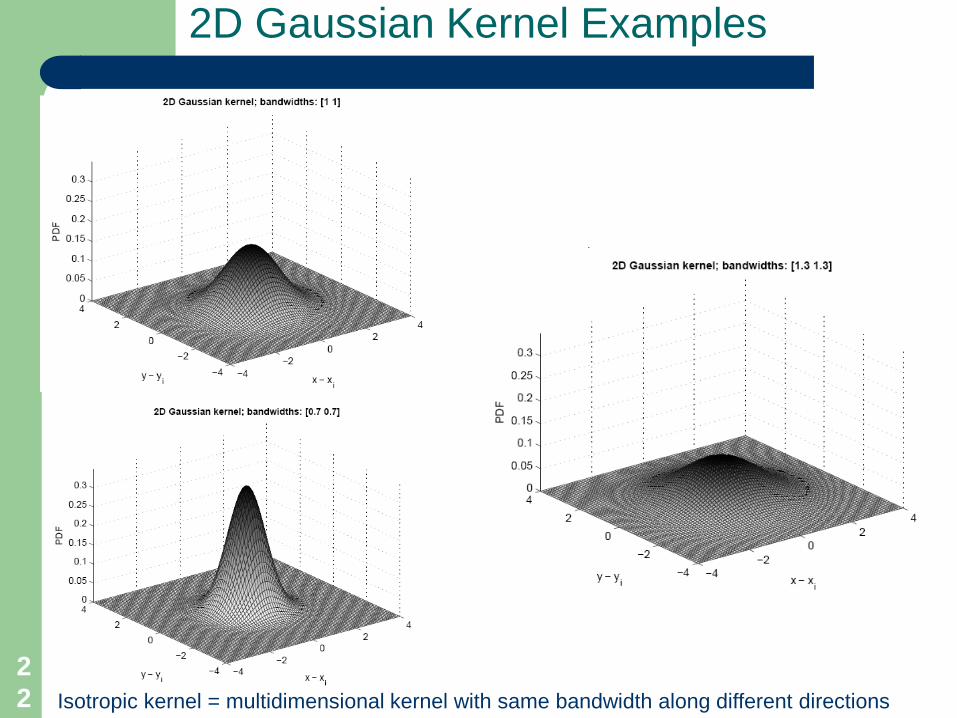
2D Gaussian Kernel Examples

Isotropic kernel = multidimensional kernel with same bandwidth along different directions

23

Multidimensional Kernel Density Estimation

Multidimensional separable kernelsK-dimensional kernels can be constructed in RK as products of K ≥2 1D kernels:

uk = k-th coordinate of location u; uik = k-th coordinate of event location ui

bj = bandwidth along k-th dimension; b = vector with K bandwidths

Estimated densityApply the same computational flowchart as in 1D:

Similar rules with 1D case exist for choosing “optimal" bandwidths along each dimension

24

2D Kernel Intensity Estimation I

1. center a circle C(u;b) of radius b at any arbitrary location u in D2. estimate local intensity at u as: λ(u) =N(u; b)/|C(u;b)|

where N(u; b) = # of events within C(u; b)|C(u; b)| = kernel measure, b2 in 2D.

Note: steps 1 and 2 amount to choosing a 2D kernel function that plots like a cylinder with base radius b and height 1=(b2)3. repeat estimation for set of points (typically arranged at the grid nodes of a regular raster) in the study region to create an intensity map

Looping over # of grid nodes (P) instead over # of events (N),yields same results as kernel density estimation case

25

2D Kernel Intensity Estimation II

conversion of point events to raster format, used for visualizing spatial patterns in event intensity and for detecting “hot spots"

resulting raster surface reveals large-scale patterns in intensity variationlarger kernel bandwidth b yields smoother intensity maps; reverse true for smaller bandwidthscould define local bandwidth b(u) as a function of presence of events in neighborhood of u; this is termed adaptive density estimationdifferent kernels, e.g., quadratic, give more weight to nearby events when calculating λ(u)Ideally, one should use some theoretical basis for selecting an appropriate kernel, e.g., a Gaussian kernel is suitable for diffusion-type processes

Example – Lung & Larynx cancer in Lancanshire county

From Bailey & Gatrell (P. 129-132), images from Tony Smith’s Spatial Data Analysis notebookhttp://www.seas.upenn.edu/~ese502/#notebookBased on data collected between 1974-1983Blue dots are lung cancer casesRed dots are larynx cancer cases

26

Example – Lung & Larynx cancer in Lancanshire county

27

Just how likely was such a cluster of cancer cases located in the sparsely populated south?Wind Direction

28

Recap

Event intensity of spatial point patternsλ(u): mean # of events over a unit area centered at uestimated overall intensity λ = N/|D|local intensity via quadrat counts or kernel density estimation

Kernel intensity estimationconversion of point data (events) to raster format (intensity surface)statistical multidimensional (multivariate) density estimation methods are used to estimate local intensity f(u). Note: Density surface integrates to 1, so multiply every such estimate f(u) by Nto convert it to an intensity value f(u)resulting intensity surface depends on: (i) kernel type, and (ii) bandwidth; the latter is more influentialalternative approaches for non-parametric multivariate density estimation include: k-nearest neighbor and mixture of Gaussian densities methodsintensity surface can be linked (via regression models) to explanatory variables, e.g., disease occurrence intensity as function of air quality variablesAn introduction to R - Venables and Smith (on site).