intelligent dasymetric mapping and its application to ... lit/mennis... · intelligent dasymetric...

Intelligent Dasymetric Mapping and Its Application to Areal Interpolation

Jeremy Mennis and Torrin Hultgren

ABSTRACT: This research presents a new “intelligent” dasymetric mapping technique (IDM), which combines an analyst’s domain knowledge with a data-driven methodology to specify the functional relationship of the ancillary classes with the underlying statistical surface being mapped. The data-driven component of IDM employs a flexible empirical sampling approach to acquire information on the data densities of individual ancillary classes, and it uses the ratio of class densities to redistribute population to sub-source zone areas. A summary statistics table characterizing the resulting dasymetric map can be used to compare the quality of the output of different IDM parameterizations. A case study of four population variables is used to demonstrate IDM and provide a visual and quantitative error assessment comparing various IDM parameterizations with areal weighting and conventional

“binary” dasymetric mapping. Intelligent dasymetric mapping outperforms areal weighting, and certain IDM parameterizations outperform binary dasymetric mapping.

Cartography and Geographic Information Science, Vol. 33, No. 3, 2006, pp. 179-194

Introduction

There has been much recent research on areal interpolation of population data. Much of this interest has been driven by

demand for small-area population estimates for regions in which only relatively coarse resolution population data can readily be obtained. Such data sets are useful in a wide range of applica-tions, such as emergency planning and manage-ment (Dobson et al. 2000), public health (Hay et al. 2005), and monitoring global population (Sutton et al. 2001). The increasing volume and availability of remotely sensed imagery, which has been shown to indicate population distribu-tion (Liu 2003; Holt et al. 2004; Wu et al. 2005), has driven much of the recent research in areal interpolation of population.

A prominent method in areal interpolation is dasymetric mapping, defined here generally as the use of an ancillary data set to disaggregate coarse resolution population data to a finer reso-lution (Eicher and Brewer 2001). Recent research suggests that dasymetric mapping can provide more accurate small-area population estimates than many areal interpolation techniques that do not use ancillary data (Mrozinski and Cromley 1999; Gregory, 2002). However, this research has not

identified an optimal methodology for specifying the functional relationship of the ancillary data with population density. In traditional dasymetric mapping approaches, this relationship has been specified subjectively by the analyst (Wright 1936; Eicher and Brewer 2001). More recently, statisti-cal methods have been used to characterize this relationship (Goodchild et al. 1993; Langford et al. 1991).

In previous research, we described the develop-ment of an algorithm for dasymetric mapping that relies on sampling the source population data to quantify the population density of individual ancillary data classes (Mennis 2003; Mennis and Hultgren 2005). Here, we extend this previous research to present a new “intelligent” dasymetric mapping (IDM) technique that supports a variety of methods for characterizing the relationship between the ancillary data and underlying statis-tical surface. We refer to the technique as intel-ligent because an analyst may: 1) establish this relationship subjectively using their own domain knowledge; 2) extract this relationship from the data using a novel empirical sampling technique; or 3) combine the subjective and empirically based methods. The IDM method is implemented as a geographic information system (GIS) extension that facilitates the parameterization of the technique and returns a set of statistics that summarize the quality of the resulting dasymetric map. As a case study, IDM is used to redistribute U.S. Census tract-level data for four population variables for the Denver, Colorado, region to sub-tract units using ancillary land cover data. U.S. Census block-level data for the same region are used to analyze the

Jeremy Mennis, Department of Geography and Urban Studies, 1115 W. Berks St., 309 Gladfelter Hall, Temple University, Philadelphia, PA 19122. Phone: (215) 204-4748, Fax: (215) 204-7388, Email: <[email protected]>. Torrin Hultgren, Department of Geography, UCB 360, University of Colorado, Boulder, CO 80309. Email: <[email protected]>.

180 Cartography and Geographic Information Science

accuracy of the derived dasymetric map. Different parameterizations of IDM are compared with other, conventional areal interpolation methods.

Previous Research in Dasymetric Mapping and Areal InterpolationTo our knowledge, the earliest reference to dasymetric mapping is the 1922 population map of European Russia by Russian cartogra-pher Semenov Tian-Shansky (for discussion, see Fabrikant’s (2003) and Bielecka’s (2005) read-ings of the work of Preobrazenski (1954) and (1956), respectively). J.K. Wright (1936) popu-larized dasymetric mapping in the U.S. and is often incorrectly cited as its inventor, though he noted the Russian origin of the term “dasymet-ric” (Wright 1936, p. 104). Modern cartography textbooks define a dasymetric map as one that displays statistical surface data by exhaustively partitioning space into zones that reflect the underlying statistical surface variation (e.g., Dent 1999; Slocum et al. 2003). Ideally, the zones in a dasymetric map should be as near to homo-geneous in character as possible, having near constant values within, and having boundaries coincident with, the surface’s steepest escarp-ments.

Dasymetric mapping as a procedure is applied to data sets for which the underlying statistical surface is unknown, but for which aggregated data already exist, though the zones of aggregation are not derived from the variation in the underly-ing statistical surface but are rather the result of some convenience of enumeration. The process of dasymetric mapping is thus the transformation of data from the arbitrary zones of data aggre-gation to a dasymetric map in order to recover and depict the underlying statistical surface. In dasymetric mapping, the transformation of data from the arbitrary zones of the original source data to the meaningful zones of the dasymetric map incorporates the use of an ancillary data set that is separate from, but related to, the variation in the statistical surface (Eicher and Brewer 2001). Dasymetric mapping therefore has a close rela-tionship to areal interpolation—the transforma-tion of data from a set of source zones to a set of target zones with different geometry (Goodchild and Lam 1980).

Recent research in dasymetric mapping has been subsumed in large measure under the topic of areal interpolation. Mrozinski and Cromley (1999) provide a helpful typology of areal interpolation

within which dasymetric mapping may be placed. The typology delineates methods for combining choropleth and area-class maps; in the latter case, zone boundaries demark regions of rela-tively homogeneous character (Mark and Csillig 1989). Mrozinski and Cromley (1999) distinguish between the “alternate geography” problem, in which areal interpolation is used to transform data from the choropleth map source zones to the area-class map target zones, and the “polygon overlay” problem, in which the target zones are formed by the intersection of the choropleth and area-class maps.

The most basic method for areal interpolation is areal weighting, in which a homogeneous distribu-tion of the data throughout each source zone is assumed. Each source zone therefore contributes to the target zone a portion of its data proportional to the percentage of its area that the target zone occupies. In the case of the alternate geography problem, if we denote a choropleth source zone s and an area-class map zone z, then the target zone t = z. The estimation of the count for the target zone is:

(1)

where:ty = the estimated count of the target zone;

ys = the count of the source zone;

zsA ∩ = the area of the intersection between the source and target zone; As = the area of the source zone; and n = the number of source zones with which z overlaps (Goodchild and Lam 1980). In the polygon overlay problem, where zst ∩=

, and each target zone intersects one and only one source zone, Equation (1) may be simplified to read:

(2)

where tA is the area of the target zone.Dasymetric mapping can be considered an

approach to the polygon overlay areal interpo-lation problem which seeks to improve on areal weighting by establishing a relationship between the underlying statistical surface and the differ-ent classes contained within the area-class map. Dasymetric areal interpolation techniques can be distinguished from other areal interpola-tion approaches that either do not make use of

∑=

∩=n

s s

zsst A

Ayy

1

ˆ

s

tst A

Ayy =ˆ

Vol. 33, No. 3 181

ancillary data or do not incorporate information regarding the different ancillary classes, such as areal weighting, distance-weighted interpolation of areal data mapped to point locations (Martin 1989), and smooth pycnophylactic interpolation (Tobler 1979).

Perhaps the most common dasymetric mapping method is the traditional binary method, in which ancillary data classes are regarded as either populated or unpopulated (Eicher and Brewer 2001). Other traditional dasymetric methods include the class percent and limiting variable methods (Wright 1936; McCleary 1969; Eicher and Brewer 2001). These traditional methods have been adapted for use with remotely sensed imagery (Mennis 2003; Holt et al. 2004) and, more recently, for road network data (Hawley and Moellering 2005; Reibel and Bufalino 2005). Other researchers have specified the relationship between the underlying statisti-cal surface and the ancillary data classes using regression (Langford et. al. 1991; Goodchild et al. 1993; Yuan et al. 1997), the expectation/maxi-mization (EM; Dempster et al. 1977) algorithm (Flowerdew et al. 1991; Bloom et al. 1996), and the use of maximum likelihood estimation in a spatial interaction model (Mrozinski and Cromley 1999).

Research which has compared a variety of areal interpolation methods suggests that dasymetric and intelligent areal interpolation techniques can outper-form areal weighting and other areal interpolation approaches that do not incorporate ancillary data (see Wu et al. (2005) for a recent review), though interpolation accuracy is dependent on both the strength of the relationship between the source and ancillary data as well as the geometry of the source, target, and ancillary data zones (Sadahiro 1999). Fisher and Langford (1995) found that the traditional binary dasymetric method was more accurate than both areal weighting and a regres-sion-based intelligent areal interpolation technique. Similar results were born out by Gregory (2002), who also demonstrated the combination of the binary method with the EM algorithm. Mrozinski and Cromley (1999) found dasymetric techniques to be more accurate than areal weighting and smooth pycnophylactic interpolation.

Intelligent Dasymetric Mapping Intelligent dasymetric mapping takes as input count data mapped to a set of source zones and a categorical ancillary data set, and redistributes the data to a set of target zones formed from the

intersection of the source and ancillary zones. Data are redistributed based on a combination of areal weighting and the relative densities of ancillary classes (Mennis 2003). Consider a source zone s and an ancillary zone z where z is associated with ancillary class c. Target zone t is defined as an area of overlap of s and z. The estimated count for a given target zone is calcu-lated as:

(3)

where cD is the estimated density of ancillary class c.

The value of cD may be set by the analyst, if the analyst has a priori knowledge of the density value for that class. Or, the analyst may choose to derive the data density for any ancillary class by sampling a subset of the total source zones that may be associated with that ancillary class. The analyst has three options for the sampling method employed. The ‘containment’ method selects those source zones that are wholly contained within an individual ancillary class. The ‘centroid’ method selects those source zones that have their centroids contained within an individual ancillary class. The ‘percent cover’ method allows the user to set a threshold percentage value and then selects those source zones whose area of occupation by a single ancillary class is equal to or exceeds that threshold. Once a sample of source zones has been selected as representative of a particular ancillary class, cD may be calculated as:

(4)

where m is the number of sampled source zones associated with ancillary class c.

Note that even when an analyst chooses to derive the density of most of the ancillary classes by sam-pling there may be one or two ancillary classes to which the analyst knows that no data should be distributed. In the case where one or more ancil-lary classes are assigned a data density of zero by the analyst, the term tA in Equation (3) refers only to the areas of target zones associated with ancillary classes that are inhabited, i.e., for which a data density of zero has not been enforced by the analyst. Likewise, the term cD in Equation (4) refers only to the densities of ancillary classes

( )

=

∑∈st

ct

ctst DA

DAyy ˆ

ˆˆ

∑∑==

=m

ss

m

ssc AyD

11/ˆ


that are inhabited. In addition, the term sA in Equation (4) is replaced by the area of the source zone occupied by inhabited ancillary classes.

To account for spatial variation in the relationship between data density and ancillary class, IDM can incorporate an additional data set of region zones, where the data density for each ancillary class is calculated separately for each individual region. There is also the possibility that a particular ancil-lary class may go unsampled, which can occur using the containment or the percent cover sampling method. In this case, the unsampled class’s density is estimated using “refined” areal weighting. First, the count assigned to each target zone associated with an unsampled class is estimated based on the previously estimated densities of the other ancillary classes that occupy that target zone’s host source zone. For instance, consider a source zone that overlaps multiple ancillary zones. Some ancillary zones are associated with an ancillary class that has gone unsampled (denoted ancillary class u) and whose density estimate is therefore unknown. The other ancillary zones are associated with an ancillary class whose density estimate is known (denoted ancillary class k), because it was derived from sampling or a preset density value assigned by the analyst. The count of a target zone associ-ated with u is calculated as:

(5)

where:

)(ˆ uty = the estimated count of the target zone associated with u;

kD = the estimated density of k;

)(ktA = the area of the target zone associated with k; and

)(utA = the area of the target zone associated with u. Note that )(ˆ uty is a temporary estimate, used

only to estimate the density of the ancillary class whose density estimate is unknown; it is not the final estimated count for that target zone. Once the value of )(ˆ uty is found, the estimated density of ancillary class u can be calculated using the formula:

(6)

where: uD = the estimated density of u; and p = the number of target zones in the entire data set associated with u.

( )

−= ∑∑

∈∈ sututut

sktktksut AAADyy

)()()(

)()()( /ˆˆ

∑∑==

=p

utut

p

ututu AyD

1)()(

1)()( /ˆˆ

ImplementationThe IDM method was programmed as a Visual Basic for Applications (VBA) script within the ArcGIS (Environmental Systems Research Institute, Inc.) GIS software package. The script prompts the user via a series of dialog boxes to load the source zone and ancillary data layers, set manual preset values for selected ancil-lary classes, and select a sampling strategy. Alternatively, the user can specify the parameter-ization of the technique using a header file. The various sampling strategies are implemented using the basic overlay operations offered by ArcGIS. One parameterization option in the spa-tial selection operation in ArcGIS supports the ability to select only those polygons in one layer that fall completely within polygons in another layer. This option was used to support contain-ment sampling, where the script loops through a series of selection functions that identify those source polygons that are wholly contained within polygons of each ancillary class. Another spatial selection parameterization option supports cen-troid sampling, using the same looping struc-ture in the script. Here, the script loops through a series of selection functions that identify those source polygons whose centroids fall within each ancillary class, essentially a point-in-polygon search (though the analytical geometry is han-dled internally by the software).

The percent cover method is a bit more com-plicated as it requires both a polygon overlay operation and a tabular summary operation. An intersect operation between the source zone layer and the ancillary data layer yields a new “inter-sect” polygon data layer, for which the area is calculated for each polygon. The script then loops through each source zone polygon, retrieves those intersect layer polygons that it contains, sums the area of the source zone polygon occupied by each ancillary class, and divides that area by the area of the entire source zone polygon to yield the percent of the source zone polygon covered by each ancillary class. Those source zone polygons that exceed the user-specified threshold for the percent cover method may be identified using a simple attribute selection operation.

When the IDM script finishes a run, it returns a dasymetric vector polygon layer with a data count and density estimates for the target zones. In addi-tion, a summary table is returned that character-izes the map layer output. This table includes information that is intended to assist the user in evaluating the relative quality of the resulting dasy-

Vol. 33, No. 3 183

metric map; it is described more fully in the case study presented below. Source code for the IDM VBA script, as well as sample data for dasymetric mapping, may be downloaded from http://astro.temple.edu/~jmennis/research/dasymetric.

Case Study Data and MethodsThe IDM method is demonstrated by dasymetric mapping variables derived from the 2000 U.S. Census at the tract-level to sub-tract units. We use U.S. Census data because they are available at nested spatial resolutions; thus we enter tract-level data into IDM and then use higher resolu-tion Census data to validate the IDM results. We emphasize that IDM is not restricted to use with U.S. Census data, or even population data, but it can be applied to the estimation of any spatially aggregated count data.

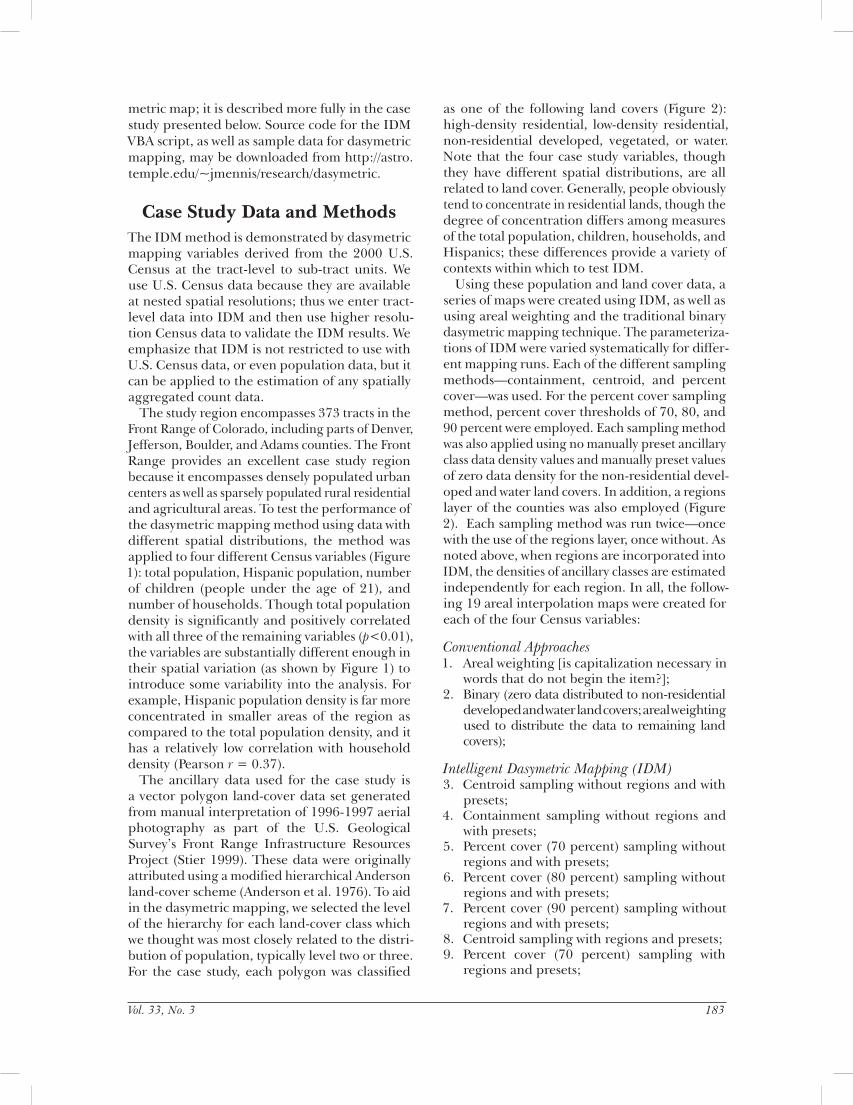
The study region encompasses 373 tracts in the Front Range of Colorado, including parts of Denver, Jefferson, Boulder, and Adams counties. The Front Range provides an excellent case study region because it encompasses densely populated urban centers as well as sparsely populated rural residential and agricultural areas. To test the performance of the dasymetric mapping method using data with different spatial distributions, the method was applied to four different Census variables (Figure 1): total population, Hispanic population, number of children (people under the age of 21), and number of households. Though total population density is significantly and positively correlated with all three of the remaining variables (p<0.01), the variables are substantially different enough in their spatial variation (as shown by Figure 1) to introduce some variability into the analysis. For example, Hispanic population density is far more concentrated in smaller areas of the region as compared to the total population density, and it has a relatively low correlation with household density (Pearson r = 0.37).

The ancillary data used for the case study is a vector polygon land-cover data set generated from manual interpretation of 1996-1997 aerial photography as part of the U.S. Geological Survey’s Front Range Infrastructure Resources Project (Stier 1999). These data were originally attributed using a modified hierarchical Anderson land-cover scheme (Anderson et al. 1976). To aid in the dasymetric mapping, we selected the level of the hierarchy for each land-cover class which we thought was most closely related to the distri-bution of population, typically level two or three. For the case study, each polygon was classified

as one of the following land covers (Figure 2): high-density residential, low-density residential, non-residential developed, vegetated, or water. Note that the four case study variables, though they have different spatial distributions, are all related to land cover. Generally, people obviously tend to concentrate in residential lands, though the degree of concentration differs among measures of the total population, children, households, and Hispanics; these differences provide a variety of contexts within which to test IDM.

Using these population and land cover data, a series of maps were created using IDM, as well as using areal weighting and the traditional binary dasymetric mapping technique. The parameteriza-tions of IDM were varied systematically for differ-ent mapping runs. Each of the different sampling methods—containment, centroid, and percent cover—was used. For the percent cover sampling method, percent cover thresholds of 70, 80, and 90 percent were employed. Each sampling method was also applied using no manually preset ancillary class data density values and manually preset values of zero data density for the non-residential devel-oped and water land covers. In addition, a regions layer of the counties was also employed (Figure 2). Each sampling method was run twice—once with the use of the regions layer, once without. As noted above, when regions are incorporated into IDM, the densities of ancillary classes are estimated independently for each region. In all, the follow-ing 19 areal interpolation maps were created for each of the four Census variables:

Conventional Approaches1. Areal weighting [is capitalization necessary in

words that do not begin the item?];2. Binary (zero data distributed to non-residential

developed and water land covers; areal weighting used to distribute the data to remaining land covers);

Intelligent Dasymetric Mapping (IDM)3. Centroid sampling without regions and with

presets;4. Containment sampling without regions and

with presets;5. Percent cover (70 percent) sampling without

regions and with presets;6. Percent cover (80 percent) sampling without

regions and with presets;7. Percent cover (90 percent) sampling without

regions and with presets;8. Centroid sampling with regions and presets;9. Percent cover (70 percent) sampling with

regions and presets;


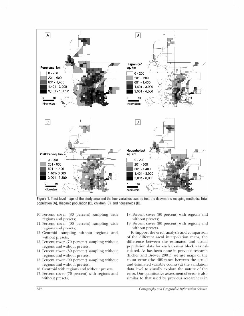
10. Percent cover (80 percent) sampling with regions and presets;

11. Percent cover (90 percent) sampling with regions and presets;

12. Centroid sampling without regions and without presets;

13. Percent cover (70 percent) sampling without regions and without presets;



16. Centroid with regions and without presets;17. Percent cover (70 percent) with regions and

without presets;

18. Percent cover (80 percent) with regions and without presets;

19. Percent cover (90 percent) with regions and without presets.

To support the error analysis and comparison of the different areal interpolation maps, the difference between the estimated and actual population data for each Census block was cal-culated. As has been done in previous research (Eicher and Brewer 2001), we use maps of the count error (the difference between the actual and estimated variable counts) at the validation data level to visually explore the nature of the error. Our quantitative assessment of error is also similar to that used by previous researchers in

Figure 1. Tract-level maps of the study area and the four variables used to test the dasymetric mapping methods: Total population (A), Hispanic population (B), children (C), and households (D).

Vol. 33, No. 3 185

its use of the root mean square (RMS) error as a summary of the error within each original source zone (Fisher and Langford 1995; Gregory 2002; Mrozinski and Cromley 1999). The error within a given source zone is calculated as:

where: RMS

sE =the RMS error of source zone s; by = the actual population of block b; by = the estimated population of block b; and q = the number of blocks contained within s.

To account for the fact that the actual population varies greatly from tract to tract, the RMS error value for each source zone is nor-malized by the actual population of the tract (Eicher and Brewer, 2001; Gregory, 2002) to derive the source zone’s coefficient of variation (CV), calculated as:

These CV scores are entered into an analysis of variance (ANOVA) test to determine whether there is a significant dif-ference in means among the CV values of the 19 different areal interpolation maps. Because the Levene statistic indicates that the assumption of homogeneity of variances among the different groups is rejected for all four vari-ables, the Tamhanes T2 post-hoc test is used to indicate whether there is a significant difference in means between each pair-wise combination of the 19 maps.

Results

Dasymetric Map OutputBecause the volume of results (including 19 areal interpola-tion maps, error maps, and summary files) is too large to present here in full, we focus on just one representative IDM output as an example before

turning to the quantitative analysis of all 19 maps. Figure 3 shows the map of total population pro-duced using the centroid sampling method with regions and presets (#8). Note that the map depicted in Figure 3 is only one visualization of the vector polygon data layer produced by the IDM run; a more detailed map could easily be generated by using a larger number of class intervals or by altering the interval boundaries. Clearly, the map presented in Figure 3 offers a far more detailed depiction of population den-sity than the analogous choropleth map shown in Figure 1. This is particularly true in subur-ban and exurban areas, where the tracts tend to be larger, and where the land cover tends to be

Figure 2. Land cover map of the study area used as the ancillary data in the dasymetric mapping methods (detail of inset box area shown at bottom). County boundaries, clipped to the study area, and county names are also shown for reference.

( )

q

yyE sb

bbRMS

s

∑∈

−=

2ˆ

(7)

(8)

s

RMSss yECV /=


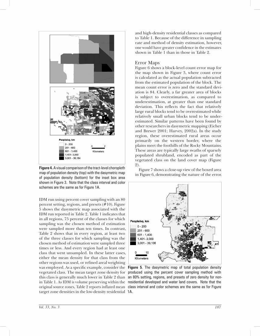
particularly heterogeneous at the transi-tion from urban to rural land uses. Figure 4 shows a close-up view of such an area (delineated as the boxed area in Figure 3) comparing the choropleth map with the IDM-derived map.

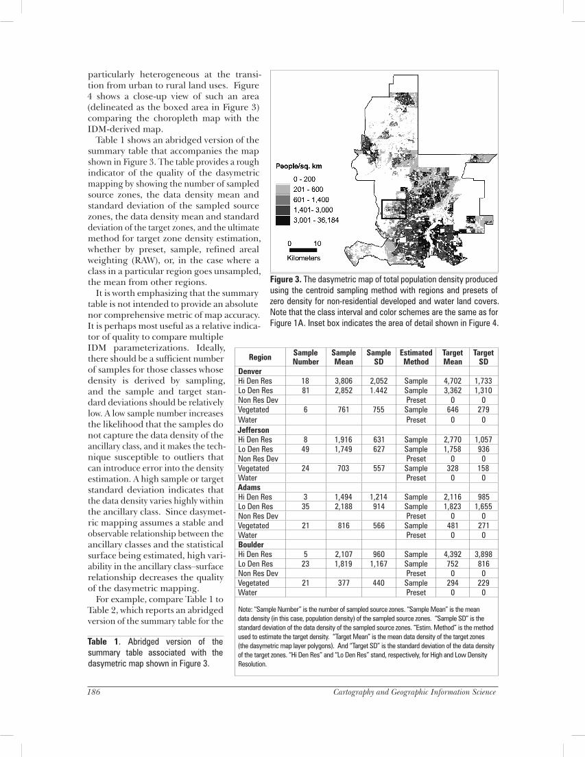
Table 1 shows an abridged version of the summary table that accompanies the map shown in Figure 3. The table provides a rough indicator of the quality of the dasymetric mapping by showing the number of sampled source zones, the data density mean and standard deviation of the sampled source zones, the data density mean and standard deviation of the target zones, and the ultimate method for target zone density estimation, whether by preset, sample, refined areal weighting (RAW), or, in the case where a class in a particular region goes unsampled, the mean from other regions.

It is worth emphasizing that the summary table is not intended to provide an absolute nor comprehensive metric of map accuracy. It is perhaps most useful as a relative indica-tor of quality to compare multiple IDM parameterizations. Ideally, there should be a sufficient number of samples for those classes whose density is derived by sampling, and the sample and target stan-dard deviations should be relatively low. A low sample number increases the likelihood that the samples do not capture the data density of the ancillary class, and it makes the tech-nique susceptible to outliers that can introduce error into the density estimation. A high sample or target standard deviation indicates that the data density varies highly within the ancillary class. Since dasymet-ric mapping assumes a stable and observable relationship between the ancillary classes and the statistical surface being estimated, high vari-ability in the ancillary class–surface relationship decreases the quality of the dasymetric mapping.

For example, compare Table 1 to Table 2, which reports an abridged version of the summary table for the

Figure 3. The dasymetric map of total population density produced using the centroid sampling method with regions and presets of zero density for non-residential developed and water land covers. Note that the class interval and color schemes are the same as for Figure 1A. Inset box indicates the area of detail shown in Figure 4.

Region Sample Number

Sample Mean

SampleSD

EstimatedMethod

TargetMean

Target SD

DenverHi Den Res 18 3,806 2,052 Sample 4,702 1,733Lo Den Res 81 2,852 1.442 Sample 3,362 1,310Non Res Dev Preset 0 0Vegetated 6 761 755 Sample 646 279Water Preset 0 0JeffersonHi Den Res 8 1,916 631 Sample 2,770 1,057Lo Den Res 49 1,749 627 Sample 1,758 936Non Res Dev Preset 0 0Vegetated 24 703 557 Sample 328 158Water Preset 0 0AdamsHi Den Res 3 1,494 1,214 Sample 2,116 985Lo Den Res 35 2,188 914 Sample 1,823 1,655Non Res Dev Preset 0 0Vegetated 21 816 566 Sample 481 271Water Preset 0 0BoulderHi Den Res 5 2,107 960 Sample 4,392 3,898Lo Den Res 23 1,819 1,167 Sample 752 816Non Res Dev Preset 0 0Vegetated 21 377 440 Sample 294 229Water Preset 0 0

Note: “Sample Number” is the number of sampled source zones. “Sample Mean” is the mean data density (in this case, population density) of the sampled source zones. “Sample SD” is the standard deviation of the data density of the sampled source zones. “Estim. Method” is the method used to estimate the target density. “Target Mean” is the mean data density of the target zones (the dasymetric map layer polygons). And “Target SD” is the standard deviation of the data density of the target zones. “Hi Den Res” and “Lo Den Res” stand, respectively, for High and Low Density Resolution.

Table 1. Abridged version of the summary table associated with the dasymetric map shown in Figure 3.

Vol. 33, No. 3 187

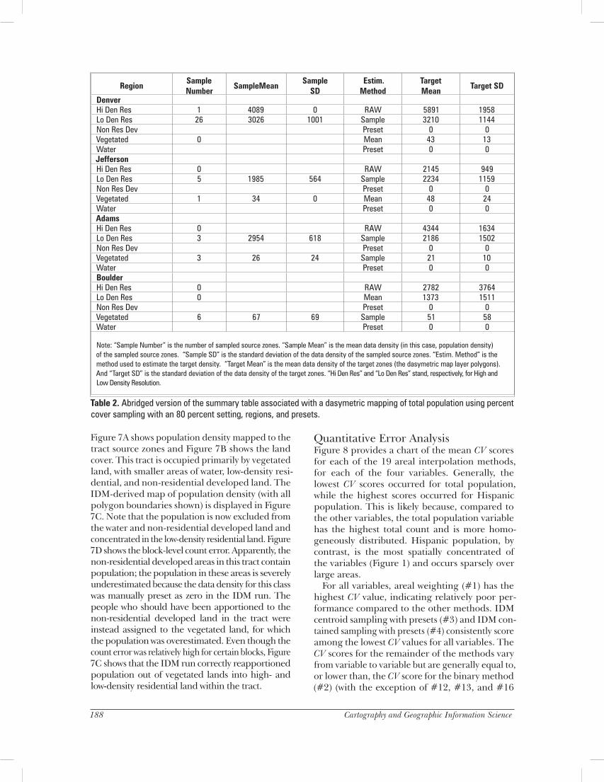
IDM run using percent cover sampling with an 80 percent setting, regions, and presets (#10). Figure 5 shows the dasymetric map associated with the IDM run reported in Table 2. Table 1 indicates that in all regions, 75 percent of the classes for which sampling was the chosen method of estimation were sampled more than ten times. In contrast, Table 2 shows that in every region, at least two of the three classes for which sampling was the chosen method of estimation were sampled three times or less. And every region had at least one class that went unsampled. In these latter cases, either the mean density for that class from the other regions was used, or refined areal weighting was employed. As a specific example, consider the vegetated class. The mean target zone density for this class is generally much lower in Table 2 than in Table 1. As IDM is volume preserving within the original source zones, Table 2 reports inflated mean target zone densities in the low-density residential

and high-density residential classes as compared to Table 1. Because of the difference in sampling rate and method of density estimation, however, one would have greater confidence in the estimates shown in Table 1 than in those in Table 2.

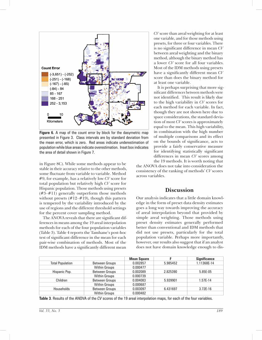
Error MapsFigure 6 shows a block-level count error map for the map shown in Figure 3, where count error is calculated as the actual population subtracted from the estimated population of the block. The mean count error is zero and the standard devi-ation is 84. Clearly, a far greater area of blocks is subject to overestimation, as compared to underestimation, at greater than one standard deviation. This reflects the fact that relatively large rural blocks tend to be overestimated while relatively small urban blocks tend to be under-estimated. Similar patterns have been found by other researchers in dasymetric mapping (Eicher and Brewer 2001; Harvey, 2002a). In the study region, these overestimated rural areas occur primarily on the western border, where the plains meet the foothills of the Rocky Mountains. These areas are typically large swaths of sparsely populated shrubland, encoded as part of the vegetated class on the land cover map (Figure 2).

Figure 7 shows a close-up view of the boxed area in Figure 6, demonstrating the nature of the error.

Figure 4. A visual comparison of the tract-level choropleth map of population density (top) with the dasymetric map of population density (bottom) for the inset box area shown in Figure 3. Note that the class interval and color schemes are the same as for Figure 1A.

Figure 5. The dasymetric map of total population density produced using the percent cover sampling method with an 80% setting, regions, and presets of zero density for non-residential developed and water land covers. Note that the class interval and color schemes are the same as for Figure 1A.


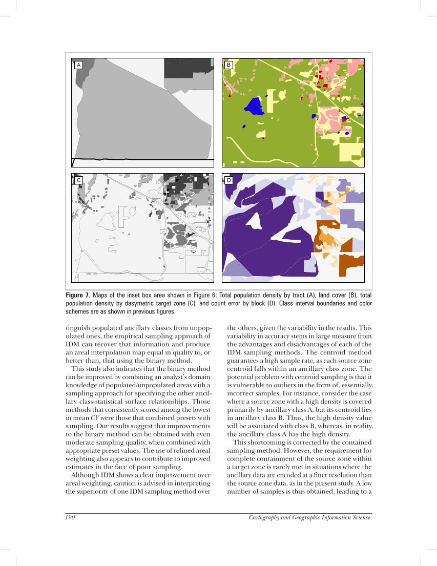
Figure 7A shows population density mapped to the tract source zones and Figure 7B shows the land cover. This tract is occupied primarily by vegetated land, with smaller areas of water, low-density resi-dential, and non-residential developed land. The IDM-derived map of population density (with all polygon boundaries shown) is displayed in Figure 7C. Note that the population is now excluded from the water and non-residential developed land and concentrated in the low-density residential land. Figure 7D shows the block-level count error. Apparently, the non-residential developed areas in this tract contain population; the population in these areas is severely underestimated because the data density for this class was manually preset as zero in the IDM run. The people who should have been apportioned to the non-residential developed land in the tract were instead assigned to the vegetated land, for which the population was overestimated. Even though the count error was relatively high for certain blocks, Figure 7C shows that the IDM run correctly reapportioned population out of vegetated lands into high- and low-density residential land within the tract.

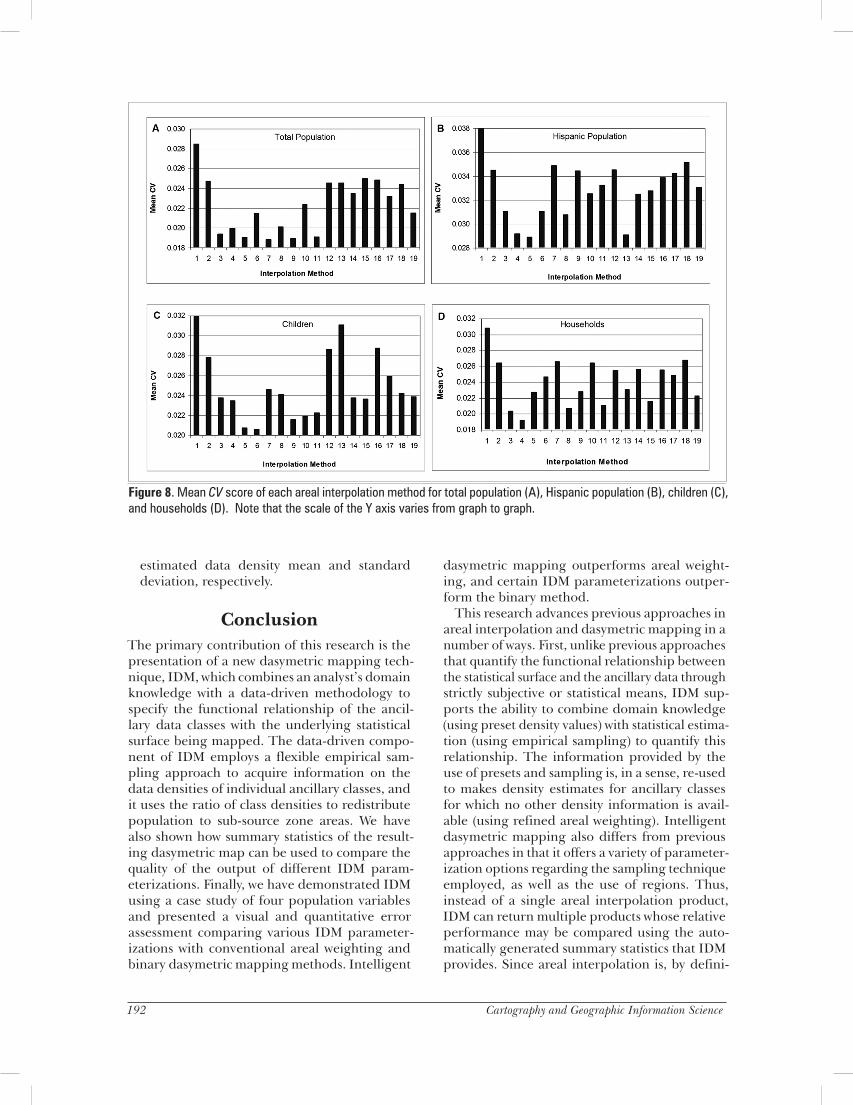
Quantitative Error AnalysisFigure 8 provides a chart of the mean CV scores for each of the 19 areal interpolation methods, for each of the four variables. Generally, the lowest CV scores occurred for total population, while the highest scores occurred for Hispanic population. This is likely because, compared to the other variables, the total population variable has the highest total count and is more homo-geneously distributed. Hispanic population, by contrast, is the most spatially concentrated of the variables (Figure 1) and occurs sparsely over large areas.

For all variables, areal weighting (#1) has the highest CV value, indicating relatively poor per-formance compared to the other methods. IDM centroid sampling with presets (#3) and IDM con-tained sampling with presets (#4) consistently score among the lowest CV values for all variables. The CV scores for the remainder of the methods vary from variable to variable but are generally equal to, or lower than, the CV score for the binary method (#2) (with the exception of #12, #13, and #16

RegionSample Number

SampleMeanSample

SDEstim.

MethodTargetMean

Target SD

DenverHi Den Res 1 4089 0 RAW 5891 1958Lo Den Res 26 3026 1001 Sample 3210 1144Non Res Dev Preset 0 0Vegetated 0 Mean 43 13Water Preset 0 0JeffersonHi Den Res 0 RAW 2145 949Lo Den Res 5 1985 564 Sample 2234 1159Non Res Dev Preset 0 0Vegetated 1 34 0 Mean 48 24Water Preset 0 0AdamsHi Den Res 0 RAW 4344 1634Lo Den Res 3 2954 618 Sample 2186 1502Non Res Dev Preset 0 0Vegetated 3 26 24 Sample 21 10Water Preset 0 0BoulderHi Den Res 0 RAW 2782 3764Lo Den Res 0 Mean 1373 1511Non Res Dev Preset 0 0Vegetated 6 67 69 Sample 51 58Water Preset 0 0

Note: “Sample Number” is the number of sampled source zones. “Sample Mean” is the mean data density (in this case, population density) of the sampled source zones. “Sample SD” is the standard deviation of the data density of the sampled source zones. “Estim. Method” is the method used to estimate the target density. “Target Mean” is the mean data density of the target zones (the dasymetric map layer polygons). And “Target SD” is the standard deviation of the data density of the target zones. “Hi Den Res” and “Lo Den Res” stand, respectively, for High and Low Density Resolution.

Table 2. Abridged version of the summary table associated with a dasymetric mapping of total population using percent cover sampling with an 80 percent setting, regions, and presets.

Vol. 33, No. 3 189

in Figure 8C). While some methods appear to be stable in their accuracy relative to the other methods, some fluctuate from variable to variable. Method #9, for example, has a relatively low CV score for total population but relatively high CV score for Hispanic population. Those methods using presets (#3–#11) generally outperform those methods without presets (#12–#19), though this pattern is tempered by the variability introduced by the use of regions and the different threshold settings for the percent cover sampling method.

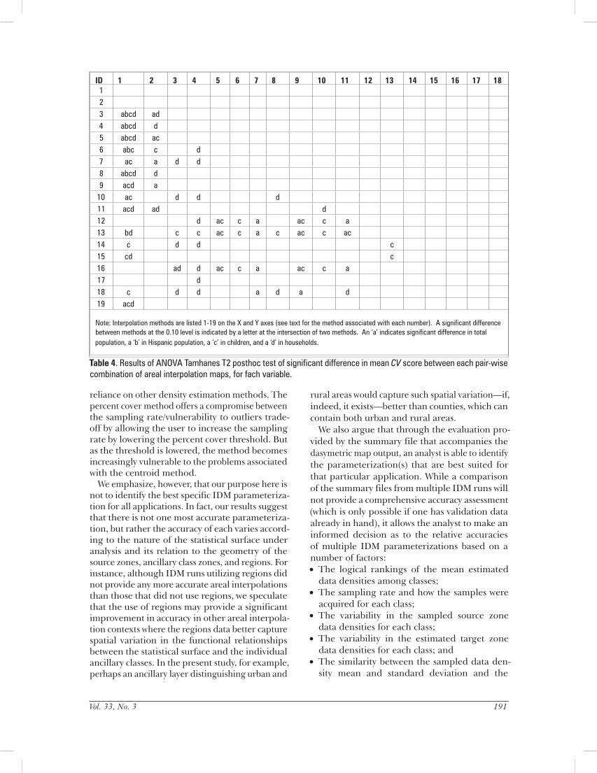
The ANOVA reveals that there are significant dif-ferences in means among the 19 areal interpolation methods for each of the four population variables (Table 3). Table 4 reports the Tamhane’s post-hoc test of significant difference in the mean for each pair-wise combination of methods. Most of the IDM methods have a significantly different mean

CV score than areal weighting for at least one variable, and for those methods using presets, for three or four variables. There is no significant difference in mean CV between areal weighting and the binary method, although the binary method has a lower CV score for all four variables. Most of the IDM methods using presets have a significantly different mean CV score than does the binary method for at least one variable.

It is perhaps surprising that more sig-nificant differences between methods were not identified. This result is likely due to the high variability in CV scores for each method for each variable. In fact, though they are not shown here due to space considerations, the standard devia-tion of most CV scores is approximately equal to the mean. This high variability, in combination with the high number of multiple comparisons and its effect on the bounds of significance, acts to provide a fairly conservative measure for identifying statistically significant differences in mean CV scores among the 19 methods. It is worth noting that

the ANOVA does not take into consideration the consistency of the ranking of methods’ CV scores across variables.

DiscussionOur analysis indicates that a little domain knowl-edge in the form of preset data density estimates goes a long way towards improving the accuracy of areal interpolation beyond that provided by simple areal weighting. Those methods using preset density estimates generally performed better than conventional and IDM methods that did not use presets, particularly for the total population variable. Perhaps more importantly, however, our results also suggest that if an analyst does not have domain knowledge enough to dis-

Figure 6. A map of the count error by block for the dasymetric map presented in Figure 3. Class intervals are by standard deviation from the mean error, which is zero. Red areas indicate underestimation of population while blue areas indicate overestimation. Inset box indicates the area of detail shown in Figure 7.

Mean Square F SignificanceTotal Population Between Groups 0.002857 5.985452 1.11368E-14

Within Groups 0.000477Hispanic Pop. Between Groups 0.002089 2.825390 5.85E-05

Within Groups 0.000739Children Between Groups 0.004083 5.939901 1.57E-14

Within Groups 0.000687Households Between Groups 0.003097 6.431697 3.72E-16

Within Groups 0.000482Table 3. Results of the ANOVA of the CV scores of the 19 areal interpolation maps, for each of the four variables.


tinguish populated ancillary classes from unpop-ulated ones, the empirical sampling approach of IDM can recover that information and produce an areal interpolation map equal in quality to, or better than, that using the binary method.

This study also indicates that the binary method can be improved by combining an analyst’s domain knowledge of populated/unpopulated areas with a sampling approach for specifying the other ancil-lary class-statistical surface relationships. Those methods that consistently scored among the lowest in mean CV were those that combined presets with sampling. Our results suggest that improvements to the binary method can be obtained with even moderate sampling quality, when combined with appropriate preset values. The use of refined areal weighting also appears to contribute to improved estimates in the face of poor sampling.

Although IDM shows a clear improvement over areal weighting, caution is advised in interpreting the superiority of one IDM sampling method over

the others, given the variability in the results. This variability in accuracy stems in large measure from the advantages and disadvantages of each of the IDM sampling methods. The centroid method guarantees a high sample rate, as each source zone centroid falls within an ancillary class zone. The potential problem with centroid sampling is that it is vulnerable to outliers in the form of, essentially, incorrect samples. For instance, consider the case where a source zone with a high density is covered primarily by ancillary class A, but its centroid lies in ancillary class B. Thus, the high density value will be associated with class B, whereas, in reality, the ancillary class A has the high density.

This shortcoming is corrected by the contained sampling method. However, the requirement for complete containment of the source zone within a target zone is rarely met in situations where the ancillary data are encoded at a finer resolution than the source zone data, as in the present study. A low number of samples is thus obtained, leading to a

Figure 7. Maps of the inset box area shown in Figure 6: Total population density by tract (A), land cover (B), total population density by dasymetric target zone (C), and count error by block (D). Class interval boundaries and color schemes are as shown in previous figures.

Vol. 33, No. 3 191

reliance on other density estimation methods. The percent cover method offers a compromise between the sampling rate/vulnerability to outliers trade-off by allowing the user to increase the sampling rate by lowering the percent cover threshold. But as the threshold is lowered, the method becomes increasingly vulnerable to the problems associated with the centroid method.

We emphasize, however, that our purpose here is not to identify the best specific IDM parameteriza-tion for all applications. In fact, our results suggest that there is not one most accurate parameteriza-tion, but rather the accuracy of each varies accord-ing to the nature of the statistical surface under analysis and its relation to the geometry of the source zones, ancillary class zones, and regions. For instance, although IDM runs utilizing regions did not provide any more accurate areal interpolations than those that did not use regions, we speculate that the use of regions may provide a significant improvement in accuracy in other areal interpola-tion contexts where the regions data better capture spatial variation in the functional relationships between the statistical surface and the individual ancillary classes. In the present study, for example, perhaps an ancillary layer distinguishing urban and

ID 1 2 3 4 5 6 7 8 9 10 11 12 13 14 15 16 17 181 2 3 abcd ad 4 abcd d 5 abcd ac 6 abc c d 7 ac a d d 8 abcd d 9 acd a

10 ac d d d 11 acd ad d 12 d ac c a ac c a 13 bd c c ac c a c ac c ac 14 c d d c 15 cd c 16 ad d ac c a ac c a 17 d 18 c d d a d a d 19 acd

Note: Interpolation methods are listed 1-19 on the X and Y axes (see text for the method associated with each number). A significant difference between methods at the 0.10 level is indicated by a letter at the intersection of two methods. An ‘a’ indicates significant difference in total population, a ‘b’ in Hispanic population, a ‘c’ in children, and a ‘d’ in households.

rural areas would capture such spatial variation—if, indeed, it exists—better than counties, which can contain both urban and rural areas.

We also argue that through the evaluation pro-vided by the summary file that accompanies the dasymetric map output, an analyst is able to identify the parameterization(s) that are best suited for that particular application. While a comparison of the summary files from multiple IDM runs will not provide a comprehensive accuracy assessment (which is only possible if one has validation data already in hand), it allows the analyst to make an informed decision as to the relative accuracies of multiple IDM parameterizations based on a number of factors:• The logical rankings of the mean estimated

data densities among classes;• The sampling rate and how the samples were

acquired for each class;• The variability in the sampled source zone

data densities for each class;• The variability in the estimated target zone

data densities for each class; and• The similarity between the sampled data den-

sity mean and standard deviation and the

Table 4. Results of ANOVA Tamhanes T2 posthoc test of significant difference in mean CV score between each pair-wise combination of areal interpolation maps, for fach variable.


estimated data density mean and standard deviation, respectively.

ConclusionThe primary contribution of this research is the presentation of a new dasymetric mapping tech-nique, IDM, which combines an analyst’s domain knowledge with a data-driven methodology to specify the functional relationship of the ancil-lary data classes with the underlying statistical surface being mapped. The data-driven compo-nent of IDM employs a flexible empirical sam-pling approach to acquire information on the data densities of individual ancillary classes, and it uses the ratio of class densities to redistribute population to sub-source zone areas. We have also shown how summary statistics of the result-ing dasymetric map can be used to compare the quality of the output of different IDM param-eterizations. Finally, we have demonstrated IDM using a case study of four population variables and presented a visual and quantitative error assessment comparing various IDM parameter-izations with conventional areal weighting and binary dasymetric mapping methods. Intelligent

dasymetric mapping outperforms areal weight-ing, and certain IDM parameterizations outper-form the binary method.

This research advances previous approaches in areal interpolation and dasymetric mapping in a number of ways. First, unlike previous approaches that quantify the functional relationship between the statistical surface and the ancillary data through strictly subjective or statistical means, IDM sup-ports the ability to combine domain knowledge (using preset density values) with statistical estima-tion (using empirical sampling) to quantify this relationship. The information provided by the use of presets and sampling is, in a sense, re-used to makes density estimates for ancillary classes for which no other density information is avail-able (using refined areal weighting). Intelligent dasymetric mapping also differs from previous approaches in that it offers a variety of parameter-ization options regarding the sampling technique employed, as well as the use of regions. Thus, instead of a single areal interpolation product, IDM can return multiple products whose relative performance may be compared using the auto-matically generated summary statistics that IDM provides. Since areal interpolation is, by defini-

Figure 8. Mean CV score of each areal interpolation method for total population (A), Hispanic population (B), children (C), and households (D). Note that the scale of the Y axis varies from graph to graph.

Vol. 33, No. 3 193

tion, an estimation procedure, information on the reliability of the estimation is key to developing useful areal interpolation products.

In future research we intend to compare IDM with other areal interpolation methods while also using different data sets. In addition to areal weighting and the binary dasymetric technique, compari-sons to the limiting variable method, expectation maximization, and other approaches would serve to further evaluate the relative performance of IDM. And although the present research used four different variables for accuracy assessment, the incorporation of other data sets for regions other than the Front Range of Colorado would be useful for evaluating the sensitivity of the accuracy assess-ment to the geometric configuration and spatial distribution of the variable being mapped.

We also intend to continue to improve the IDM methodology. First, we believe a key strength of IDM is the ability to integrate the analyst’s domain knowledge with information derived from data analysis. This integration may be enhanced by providing more sophisticated modes of user interac-tion, for instance by allowing the analyst to manu-ally select samples for certain classes through a graphical user interface (GUI), as in a supervised classification of remotely sensed imagery (Lillesand and Kiefer 2004). In addition, though the current implementation uses the ratio of data densities to specify the functional relationship between the ancillary classes and the statistical surface there is no reason that other statistical methods, such as regression, cannot be utilized in the same manner. A promising advance in this regard is reported by Harvey (2002b), who describes a two-stage approach where the binary method is initially applied, then followed by a regression-based iterative refinement to redistribute population within the populated areas. Finally, we plan to explore the possibility of using the information contained in the summary table to optimize the IDM parameterization. For this purpose, an overall index of quality incorpo-rating various components of the summary table may be generated and an optimization algorithm applied to iteratively refine the parameter settings to maximize the index value.

REFERENCESAnderson, I.R, E.E. Hardy, J.T. Roach, and R. E.

Witmer. 1976. A land use and land cover classifica-tion system for use with remote sensor data. U.S. Geological Survey Professional Paper 964. Reston, Virginia, U.S.A.

Bielecka, E. 2005. A dasymetric population density map of Poland.” In: Proceedings of the International

Cartographic Conference, July 9-15, A Coruña, Spain [CD].

Bloom, L. M., P.J. Pedler, and G.E. Wragg. 1996. Implementation of enhanced areal interpolation using Mapinfo. Computers and Geosciences 22: 459-66.

Dempster, A. P., N.M. Laird, and D.B. Rubin. 1977. Maximum likelihood from incomplete data via the EM algorithm. Journal of the Royal Statistical Society B 39: 1-38.

Dent, B. D. 1999, Cartography: Thematic map design, 5th ed. Boston, Massachusetts: WCB/McGraw-Hill.

Dobson, J. E., E. A. Bright, P.R. Coleman, R.C. Durfee, B.A. Worley. 2000. LandScan: A global popula-tion database for estimating populations at risk. Photogrammetric Engineering and Remote Sensing 66: 849-57.

Eicher, C. L., and C.A. Brewer. 2001. Dasymetric map-ping and areal interpolation: Implementation and evaluation. Cartography and Geographic Information Science 28: 125-138.

Fabrikant, S. I. 2003. Commentary on ‘A History of Twentieth-Century American Academic Cartography’ by Robert McMaster and Susanna McMaster. Cartography and Geographic Information Science 30: 81-4.

Fisher, P. F., and M. Langford. 1995. Modelling the errors in areal interpolation between zonal sys-tems by Monte Carlo simulation. Environment and Planning A 27: 211-24.

Flowerdew, R., M. Green, and E. Kehris. 1991. Using areal interpolation methods in geographic informa-tion systems. Papers in Regional Science 70: 303-15.

Goodchild, M. F., L. Anselin, and U. Deichmann. 1993. A framework for the areal interpolation of socioeconomic data. Environment and Planning A 25: 383-97.

Goodchild, M. F., and N.S. Lam. 1980. Areal interpo-lation: A variant of the traditional spatial problem. Geo-processing 1: 297-312.

Gregory, I. N. 2002. The accuracy of areal interpola-tion techniques: standardizing 19th and 20th century census data to allow long-term comparisons. Computers, Environment and Urban Systems 26: 293-314.

Harvey, J. T. 2002a. Estimating census district popula-tions from satellite imagery: Some approaches and limitations. International Journal of Remote Sensing 23: 2071-95.

Harvey, J. T. 2002b. Population estimation models based on individual TM pixels. Photogrammetric Engineering and Remote Sensing 68: 1181-92.

Hawley, K., and H. Moellering. 2005. A comparative analysis of areal interpolation methods. Cartography and Geographic Information Science 32: 411-23.

Hay, S. I., A. M. Noor, A. Nelson, and A.J. Tatem., 2005. The accuracy of human population maps for public health application. Tropical Medicine and International Health 10: 1073-86.

Holt, J. B., C.P. Lo, and T.W. Hodler. 2004. Dasymetric estimation of population density and areal interpo-


lation of Census data. Cartography and Geographic Information Science 31: 103-21.

Langford, M., D.J. Maguire, and D.J. Unwin. 1991. The areal interpolation problem: estimating pop-ulation using remote sensing in a GIS framework. In: Handling Geographic Information. Essex, U.K.: Longman Scientific and Technical. pp. 55-77.

Lillesand, T. M., and R.W. Kiefer. 2004. Remote sensing and image interpretation, 5th ed. New York, New York: John Wiley and Sons.

Liu, X. 2003. Estimation of the spatial distribution of urban population using high spatial resolution satellite imagery. Unpublished Ph.D. Dissertation, University of California Santa Barbara.

Mark, D M and Csillig, F, 1989, “The nature of bound-aries on area-class maps” Cartographica 26 65-78.

Martin, D. 1989. Mapping population data from zone centroid locations.” Transactions of the Institute of British Geographers 14: 90-7.

McCleary, G. F., Jr. 1969. The dasymetric method in the thematic cartography. Unpublished Ph.D. dis-sertation, University of Wisconsin.

Mennis, J. 2003. Generating surface models of popu-lation using dasymetric mapping. The Professional Geographer 55: 31-42.

Mennis, J., and T. Hultgren. 2005. Dasymetric map-ping for disaggregating coarse resolution popu-lation data. In: Proceedings of the International Cartographic Conference, July 9-15, A Coruña, Spain (CD).

Mrozinski, R. D., Jr., and R.G. Cromley. 1999. Singly—and doubly—constrained methods of areal interpo-lation for vector-based GIS. Transactions in GIS 3: 285-301.

Preobrazenski, A. 1954. Dorewolucjonnyje i sovietskije karty razmieszczenija nasielenia. Woprosy Geografii Kartographia 34: 134-49.

Preobrazenski, A. 1956. Okonomische Kartographie. Gotha, Germany: VEB Hermann Haack.

Reibel, M., and M.E. Bufalino. 2005. Street-weighted interpolation techniques for demographic count estimation in incompatible zone systems. Environment and Planning A 37: 127-39.

Sadahiro, Y. 1999. Accuracy of areal interpolation: A comparison of alternative methods. Journal of Geographical Systems 1: 323-46.

Slocum, T., R.B. McMaster, F.C. Kessler, and H.H. Howard. 2003. Thematic cartography and geographic visualization, 2nd ed. Upper Saddle River, New Jersey : Prentice Hall.

Stier, M.1999. Temporal land use and land cover map-ping. Paper presented at the American Society for Photogrammetry and Remote Sensing (ASPRS) Conference, Portland, Oregon. [http://rockyweb.cr.usgs.gov/frontrange/publications.htm; accessed January 3, 2006].

Sutton, P., D. Roberts, C.D. Elvidge, and K. Baugh. 2001. Census from heaven: An estimate of the global human population using night-time satellite imagery. International Journal of Remote Sensing 22: 3061-76.

Tobler, W. 1979. Smooth pycnophylactic interpolation for geographical regions. Journal of the American Statistical Association 74: 519-30.

Wright, J. K. 1936. A method of mapping densities of population. The Geographical Review 26: 103-110.

Wu, S-S., X. Qiu, and L. Wang. 2005. Population estimation methods in GIS and remote sensing: A review” GIScience and Remote Sensing 42: 80-96.

Yuan, Y., R. M. Smith, and W.F. Limp. 1997. Remodeling census population with spatial infor-mation from Landsat TM imagery. Computers, Environment and Urban Systems 21: 245-58.

intelligent dasymetric mapping and its application to ... lit/mennis... · intelligent dasymetric...

Documents