ACCELERATED IMPLEMENTATION OF

INTELLIGENT COMPACTION TECHNOLOGY

FOR EMBANKMENT SUBGRADE SOILS, AGGREGATE BASE, AND ASPHALT PAVEMENT

MATERIALS

Draft Final Report

Texas DOT FM156 Field Project July 20 to 25, 2008

Prepared By

David J. White, Ph.D. Pavana Vennapusa Heath Gieselman Luke Johansen

Rachel Goldsmith

Earthworks Engineering Research Center (EERC) Department of Civil Construction and Environmental Engineering

Iowa State University 2711 South Loop Drive, Suite 4700

Ames, IA 50010-8664 Phone: 515-294-1463 www.ctre.iastate.edu

November 25, 2008

ii

TABLE OF CONTENTS

ACKNOWLEDGMENTS ...............................................................................................................6 

INTRODUCTION ...........................................................................................................................7 

BACKGROUND .............................................................................................................................7 

Roller-Integrated Stiffness (ks) Measurement Value .................................................................. 7 Roller-Integrated Compaction Meter Value (CMV) ................................................................... 9 

EXPERIMENTAL TESTING .......................................................................................................10 

Description of Test Beds ........................................................................................................... 10 In-situ Testing Methods ............................................................................................................ 12 

IN-SITU TEST RESULTS AND DISCUSSION ..........................................................................14 

TBs 1 and 3 – Clay Subgrade Material ..................................................................................... 14 Construction of TBs ...........................................................................................................14 Roller-integrated and in-situ point measurements .............................................................15 Summary ............................................................................................................................16 

TB 2 lime-stabilized subgrade and flex base material .............................................................. 25 Construction and testing on TB2 .......................................................................................25 Roller-integrated and in-situ point measurements .............................................................25 Summary ............................................................................................................................25 

TB 5 lime-stabilized subgrade material .................................................................................... 30 Construction of TB ............................................................................................................30 Roller-integrated and in-situ point measurements .............................................................33 Summary ............................................................................................................................34 

TBs 6 and 7 flex base material .................................................................................................. 41 Construction and material conditions ................................................................................41 Roller-integrated and in-situ point measurements .............................................................42 Spatial analysis of roller-integrated and in-situ compaction measurements ......................52 Summary ............................................................................................................................54 

Comparison between padfoot and smooth drum measurements – TBs 1, 3, 4, and 5 .............. 54 

FIELD DEMONSTRATION .........................................................................................................57 

SUMMARY AND CONCLUSIONS ............................................................................................57 

REFERENCES ..............................................................................................................................60 

APPENDIX ....................................................................................................................................61 

iii

LIST OF FIGURES Figure 1. SV212 padfoot and smooth drum rollers used on the project ..........................................8 Figure 2. Lumped parameter two-degree-of-freedom spring dashpot model representing vibratory

compactor and soil behavior (reproduced from Yoo and Selig 1980) .................................8 Figure 3. Figure showing the effect of contact footprint on padfoot and smooth drum ks

measurements (Anderegg 2008) ..........................................................................................9 Figure 4. CA-362 smooth drum roller used on the project ............................................................10 Figure 5. In-situ testing methods used on the project: (a) 200-mm diameter plate Zorn LWD, (b)

dynamic cone penetrometer, (c) calibrated nuclear moisture-density gauge, (d) 300-mm diameter Dynatest FWD, (e) 300-mm diameter static PLT, (f) D-SPA, and (g) Iowa State University geotechnical mobile lab ...................................................................................13 

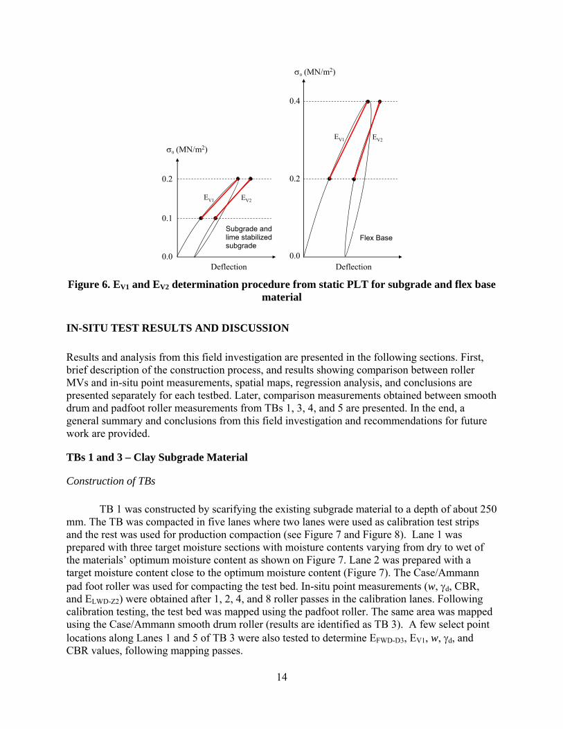
Figure 6. EV1 and EV2 determination procedure from static PLT for subgrade and flex base material ..............................................................................................................................14 

Figure 7. Experimental testing setup TB 1 ....................................................................................15 Figure 8. Picture showing different lanes on TB 1 ........................................................................15 Figure 9. kSΙPD measurement from different passes on TB1 lanes 1 and 5 (nominal a = 0.8 mm, f

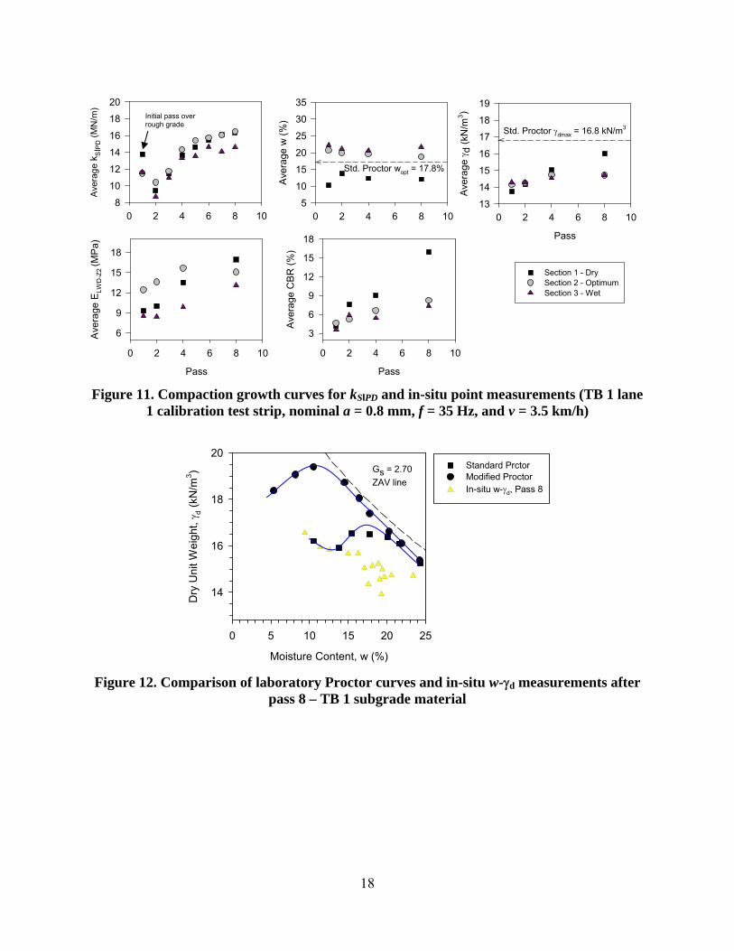
= 35 Hz, and v = 3.5 km/h) ................................................................................................17 Figure 10. Screen shots of kSΙPD maps for different passes on TB 1 ..............................................17 Figure 11. Compaction growth curves for kSΙPD and in-situ point measurements (TB 1 lane 1

calibration test strip, nominal a = 0.8 mm, f = 35 Hz, and v = 3.5 km/h) ..........................18 Figure 12. Comparison of laboratory Proctor curves and in-situ w-d measurements after pass 8 –

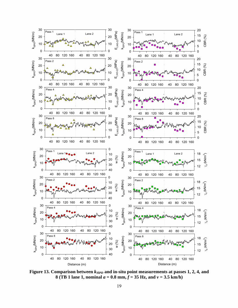
TB 1 subgrade material ......................................................................................................18 Figure 13. Comparison between kSΙPD and in-situ point measurements at passes 1, 2, 4, and 8 (TB

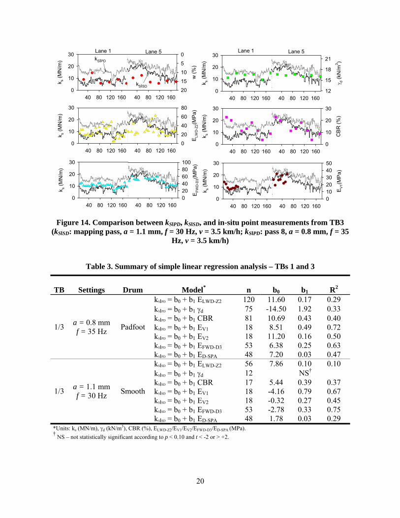
1 lane 1, nominal a = 0.8 mm, f = 35 Hz, and v = 3.5 km/h) .............................................19 Figure 14. Comparison between kSΙPD, kSΙSD, and in-situ point measurements from TB3 (kSΙSD:

mapping pass, a = 1.1 mm, f = 30 Hz, v = 3.5 km/h; kSΙPD: pass 8, a = 0.8 mm, f = 35 Hz, v = 3.5 km/h) ......................................................................................................................20 

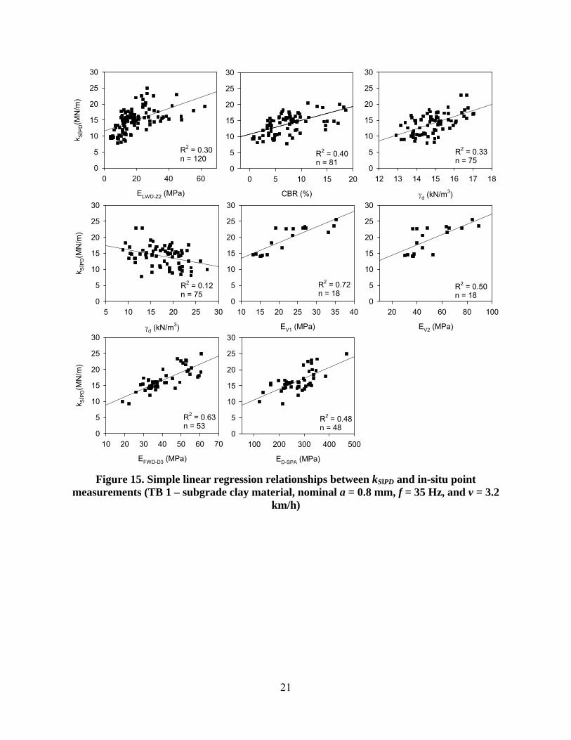
Figure 15. Simple linear regression relationships between kSΙPD and in-situ point measurements (TB 1 – subgrade clay material, nominal a = 0.8 mm, f = 35 Hz, and v = 3.2 km/h) ........21 

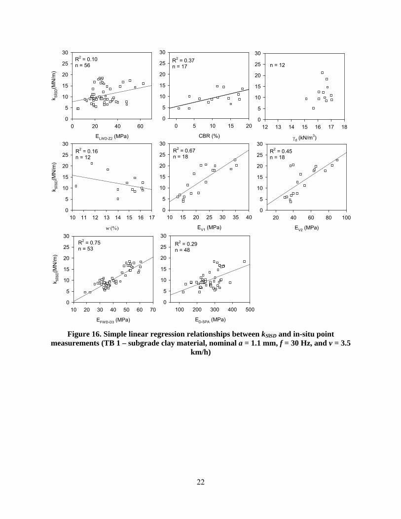
Figure 16. Simple linear regression relationships between kSΙSD and in-situ point measurements (TB 1 – subgrade clay material, nominal a = 1.1 mm, f = 30 Hz, and v = 3.5 km/h) ........22 

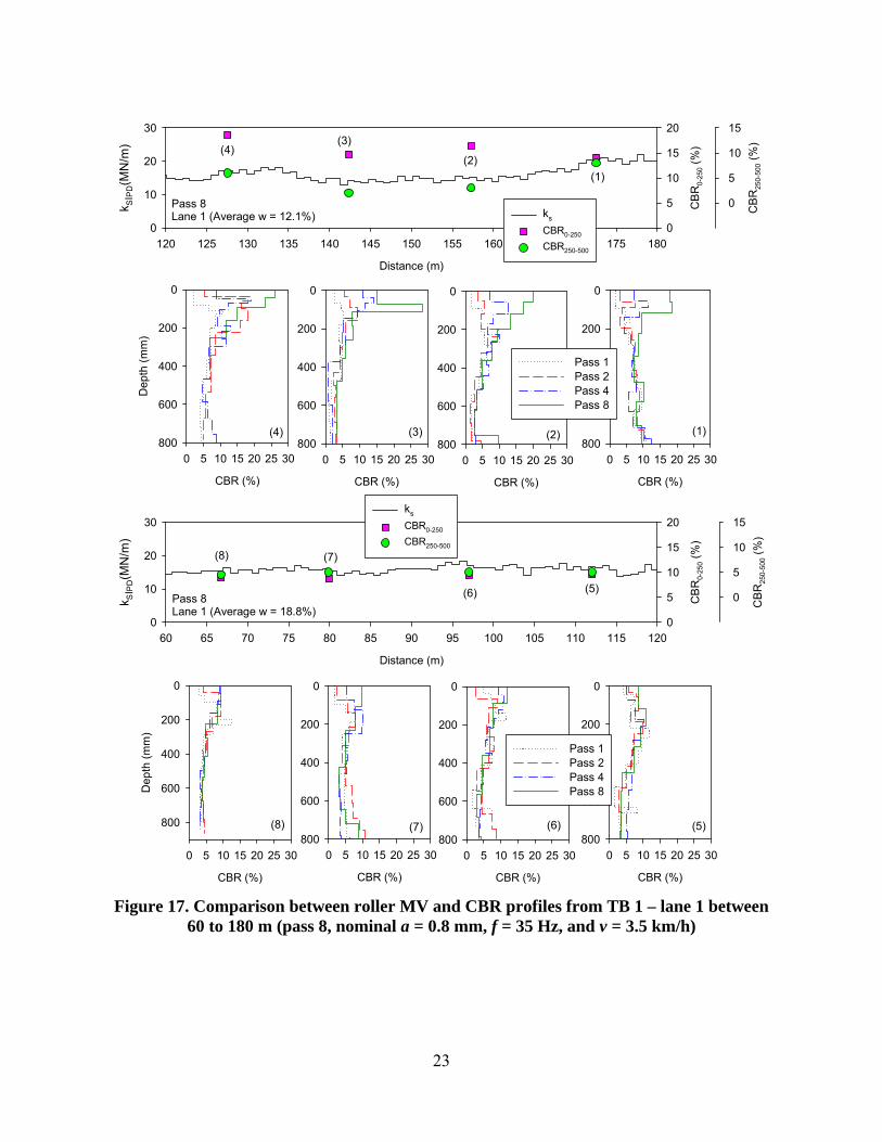
Figure 17. Comparison between roller MV and CBR profiles from TB 1 – lane 1 between 60 to 180 m (pass 8, nominal a = 0.8 mm, f = 35 Hz, and v = 3.5 km/h) ...................................23 

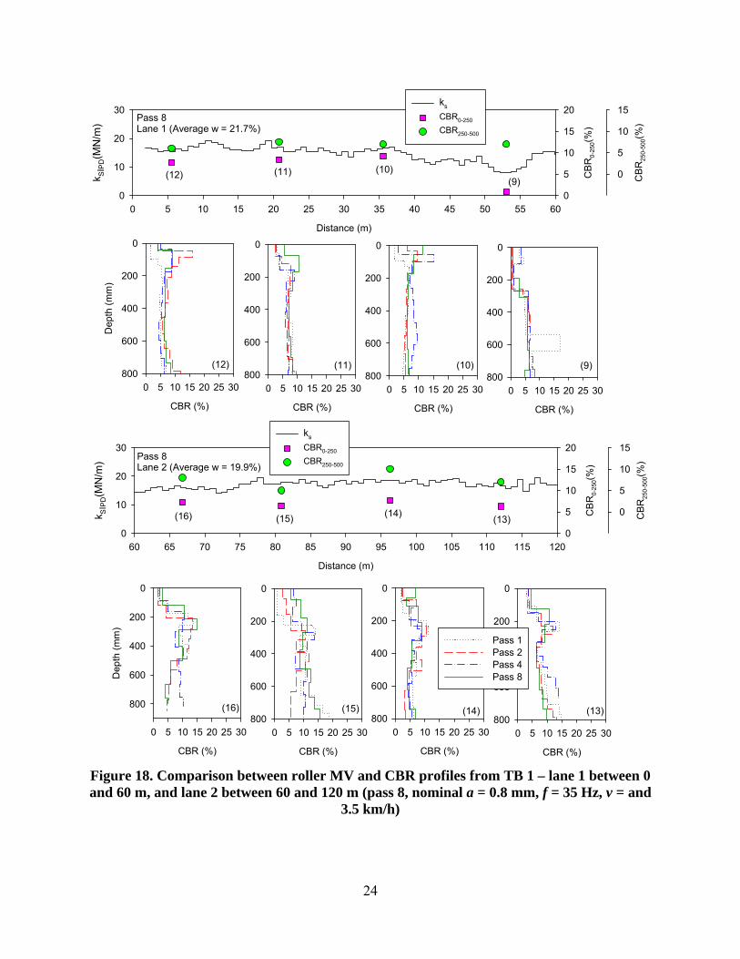
Figure 18. Comparison between roller MV and CBR profiles from TB 1 – lane 1 between 0 and 60 m, and lane 2 between 60 and 120 m (pass 8, nominal a = 0.8 mm, f = 35 Hz, v = and 3.5 km/h) ............................................................................................................................24 

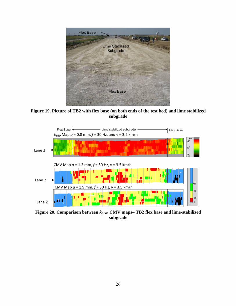
Figure 19. Picture of TB2 with flex base (on both ends of the test bed) and lime stabilized subgrade .............................................................................................................................26 

Figure 20. Comparison between kSΙSD CMV maps– TB2 flex base and lime-stabilized subgrade 26 Figure 21. Comparison between kSΙSD and in-situ point measurements – TB2 (lane 2) flex base

and lime stabilized subgrade (nominal a = 0.8 mm, f = 30 Hz, and v = 3.2 km/h) ............27 Figure 22. Comparison between CMV and in-situ point measurements – TB2 (lane 2) flex base

and lime-stabilized subgrade (nominal f = 30 Hz and v = 3.2 km/h) .................................28 Figure 23. Simple linear regression relationships between (a) kSΙPD, (b) CMV and in-situ point

measurements – TB 2.........................................................................................................29 

iv

Figure 24. Photos showing placement (left) and reclamation (right) process of lime slurry with existing subgrade material (pictures taken 07/21/08) ........................................................31 

Figure 25. Picture showing ponding of lime slurry on the scarified subgrade (picture taken 07/21/2008) ........................................................................................................................31 

Figure 26. Picture showing soil reclaiming (left) and moisture conditioning process on TB 5 (picture taken 07/23/2008) .................................................................................................32 

Figure 27. Experimental testing setup on TB5 (lane 3 for padfoot roller calibration strip and lane 4 for smooth drum roller calibration strip) ........................................................................32 

Figure 28. Picture of TB5 with different lanes ..............................................................................32 Figure 29. Comparison of laboratory Proctor curves and in-situ w-d measurements – TB 5 lime-

stabilized subgrade material ...............................................................................................33 Figure 30. kSΙPD measurements from different passes on TB5 lane 3 calibration test strip (nominal

a = 1.0 mm, f = 35 Hz, and v = 3.5 km/h) ..........................................................................35 Figure 31. Compaction growth curves for kSΙPD and in-situ point measurements (TB 5 lane 3

calibration test strip, nominal a = 1.0 mm, f = 35 Hz, and v = 3.5 km/h) ..........................35 Figure 32. Compaction growth curves for in-situ point measurements (TB 5 lane 4 calibration

test strip) (*roller data file corrupt) ....................................................................................35 Figure 33. Comparison results between kSΙPD (passes 1 to 12), kSΙSD (pass 13), and in-situ point

measurements – TB5 lime stabilized subgrade calibration lane (nominal a = 1.0 mm, f = 35 Hz, and v = 3.5 km/h) ...................................................................................................36 

Figure 34. Comparison between kSΙPD, kSΙSD, and in-situ point measurements on TB 5 – lane 1 lime stabilized subgrade material (kSΙPD: nominal a = 1.0 mm, f = 35 Hz, and v = 3.5 km/h; kSΙSD: nominal a = 1.5 mm, f = 35 Hz, and v = 3.2 km/h) ........................................37 

Figure 35. kSΙSD maps (map 1: nominal a = 1.5 mm, f = 30 Hz, and v = 3.2 km/h) and DCP profiles at select locations on TB5 lime stabilized material (isolated area underlain by a concrete box culvert) ..........................................................................................................38 

Figure 36. Simple linear regression relationships between kSΙPD and in-situ point measurements (TB 5 – lime stabilized subgrade clay material, nominal a = 1.0 mm, f = 35 Hz, and v = 3.2 km/h) ............................................................................................................................39 

Figure 37. Simple linear regression relationships between kSΙSD and in-situ point measurements (TB 5 – lime stabilized subgrade clay material, nominal a = 1.5 mm, f = 30 Hz, and v = 3.2 km/h) ............................................................................................................................40 

Figure 38. Experimental setup on TB 6 .........................................................................................42 Figure 39. Moisture on flex base material during compaction (TB 6 left) and a day after

compaction (TB 7 right) .....................................................................................................42 Figure 40. Moisture segregation on flex base material during testing (TB 7) ...............................42 Figure 41. CMV and BV values for compaction passes on lane 1 of TB6 flex base material ......44 Figure 42. CMV and BV values for compaction passes on lane 2 of TB6 flex base material ......44 Figure 43. CMV and BV values for compaction passes on lane 3 of TB6 flex base material ......45 Figure 44. CMV, BV, and a values for compaction passes on lane 4 of TB6 flex base material .46 Figure 45. CMV and BV values for compaction passes on lane 5 of TB6 flex base material ......46 Figure 46. CMV compaction growth curves for TB 6 lanes 1 to 5 ...............................................47 Figure 47. CMV maps on TB 7 with different operation settings .................................................47 Figure 48. Comparison between CMV and in-situ point measurements (EFWD, d, and w) on TB 7

flex base material flex base material (nominal f = 30 Hz, v = 3.5 km/h) ...........................48 Figure 49. Comparison between CMV and point measurements (ED-SPA and EV1) on TB 7 flex

base material flex base material (f = 30 Hz, v = 3.5 km/h) ................................................49 

v

Figure 50. Comparison between CMV and DCP measurements on lanes 1 and 3 of TB 7 flex base material (nominal f = 30 Hz, v = 3.5 km/h) ...............................................................50 

Figure 51. Comparison between CMV measurements in manual and automatic settings (nominal f = 30 Hz, v = 3.5 km/h) .....................................................................................................51 

Figure 52. Kriged contour maps and semi-variograms of CMV and EFWD on TB 7 flex base material ..............................................................................................................................53 

Figure 53. Comparison between kSΙPD and kSΙSD measurements (TB 1 – subgrade clay material) .55 Figure 54. Comparison between kSΙPD and kSΙSD measurements (TB 4 – flex base material and TB

5 – lime stabilized subgrade material) ...............................................................................56 Figure 55. Spatial comparison of kSΙPD and kSΙSD maps (TB 1 – subgrade clay material) ..............56 Figure 56. Relationship between kSΙPD and kSΙSD measurements ....................................................57 

LIST OF TABLES Table 1. Summary of test beds and in-situ testing .........................................................................11 Table 2. Summary of soil index properties ....................................................................................11 Table 3. Summary of simple linear regression analysis – TBs 1 and 3 .........................................20 Table 4. Summary of simple linear regression analysis – TB 2 ....................................................30 Table 5. Summary of simple linear regression analysis – TB 5 ....................................................41 

6

ACKNOWLEDGMENTS

This study was funded by US FHWA research project DTFH61-07-C-R0032 “Accelerated Implementation of Intelligent Compaction Technology for Embankment Subgrade Soils, Aggregate Base, and Asphalt Pavement Materials”. Zhiming Si, Robert L. Graham, and Richard Williammee with TXDOT provide project coordination and assistance with field testing. Stan Allen served as the contractor liaison for Ed Bell Construction Co. Kirby Carpenter from Texana Machinery/Case, Rolland Anderegg with Ammann Compaction Ltd. (Switzerland), and Gert Hanson with Dynapac USA, Inc. provided intelligent compaction rollers and field support during the project. D-SPA tests were conducted by Prof. Soheil Nazarian and Mr. Deren Yuan from the University of Texas at El Paso. George Chang from the Transtec Group, Inc. is the Principal Investigator for this research project. Robert D. Horan is the project facilitator and assisted with scheduling rollers for the project. Many other assisted with the coordination and participated in the field demonstrations and their assistance and interest is greatly appreciated.

7

INTRODUCTION

The Iowa State University research team conducted field investigations on the FM156 project located in Roanoke, Texas from June 20 – 25, 2008 on Case/Ammann and Dynapac intelligent compaction (IC) rollers. The project involved preparing and testing seven test beds with Type II, III, and V materials (Type II – fine-grained cohesive subgrade clay, Type V – lime stabilized subgrade, and Type III – flex base aggregate material) as identified in the project proposal. Case/Ammann smooth drum and padfoot rollers equipped with roller-integrated stiffness (ks) and Dynapac smooth drum roller equipped with roller-integrated CMV measurement systems were used on the project. The rollers were equipped with GPS and on-board documentation systems. Goals of this field investigation were to:

Evaluate the effectiveness of the roller-integrated measurement values (MVs) from

padfoot and smooth drum rollers in assessing the compaction quality of three material types (Type II, III and V) encountered on the project,

Develop correlations between MVs from padfoot and smooth drum rollers and various conventionally used in-situ point measurements in QC/QA practice, and

Assess comparisons between smooth drum and padfoot roller MVs. This report presents background information for the two measurement systems evaluated in this study (ks and CMV), and documents the results and analysis from test bed field studies and the field demonstration activities. Results presented in this report for the padfoot roller are of high priority among many state DOTs and contractor personnel (based on a recent survey conducted by White 2008). To the authors’ knowledge, this is the first documented field study to report accelerometer based padfoot roller MVs applications for fine grained cohesive subgrade and lime stabilized subgrade materials, and comparison of padfoot to smooth drum roller MVs. These results should be of significant interest to the pavement, geotechnical, and construction engineering community and are anticipated to promote implementation of compaction monitoring technologies into earthwork construction practice in the United States. Further the results of smooth drum measurements for the Type III flex base aggregate material provided new correlation results. BACKGROUND

Roller-Integrated Stiffness (ks) Measurement Value

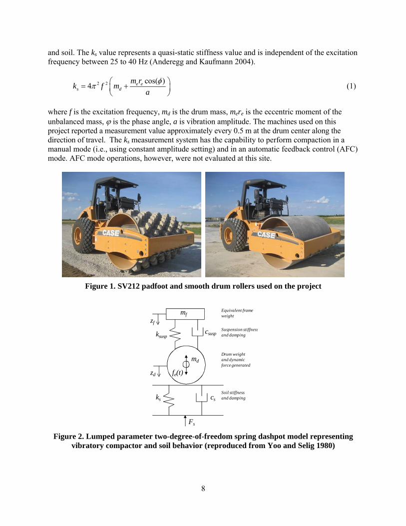
SV-212 12-ton padfoot and smooth drum Case rollers equipped with Ammann’s roller-integrated stiffness ks measurement value were used on this project (Figure 1). The ks measurement system was introduced by Ammann during late 1990’s considering a lumped parameter two-degree-of-freedom spring dashpot system illustrated in Figure 2 (Anderegg 1998). The spring dashpot model has been found effective in representing the drum-ground interaction behavior (Yoo and Selig 1980). The drum inertia force and eccentric force time histories are determined from drum acceleration and eccentric position (neglecting frame inertia). The drum displacement zd is determined by double integrating the measured peak drum accelerations. The soil stiffness ks is determined using Equation 1 when there is no loss of contact between drum

8

and soil. The ks value represents a quasi-static stiffness value and is independent of the excitation frequency between 25 to 40 Hz (Anderegg and Kaufmann 2004).

2 2 cos( )4 e e

s d

m rk f m

a

(1)

where f is the excitation frequency, md is the drum mass, mere is the eccentric moment of the unbalanced mass, is the phase angle, a is vibration amplitude. The machines used on this project reported a measurement value approximately every 0.5 m at the drum center along the direction of travel. The ks measurement system has the capability to perform compaction in a manual mode (i.e., using constant amplitude setting) and in an automatic feedback control (AFC) mode. AFC mode operations, however, were not evaluated at this site.

Figure 1. SV212 padfoot and smooth drum rollers used on the project

zd

csks

mf

ksuspcsusp

fe(t)

zf

Equivalent frame weight

Suspension stiffnessand damping

Drum weightand dynamicforce generated

Soil stiffnessand damping

md

Fs

Figure 2. Lumped parameter two-degree-of-freedom spring dashpot model representing vibratory compactor and soil behavior (reproduced from Yoo and Selig 1980)

9

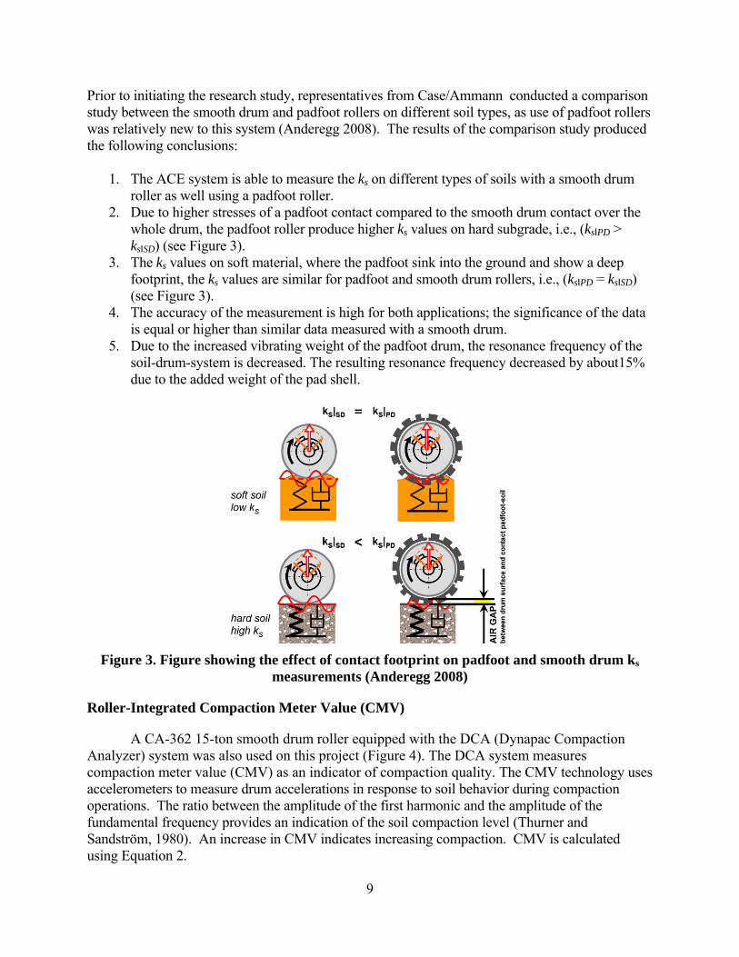
Prior to initiating the research study, representatives from Case/Ammann conducted a comparison study between the smooth drum and padfoot rollers on different soil types, as use of padfoot rollers was relatively new to this system (Anderegg 2008). The results of the comparison study produced the following conclusions:

1. The ACE system is able to measure the ks on different types of soils with a smooth drum roller as well using a padfoot roller.

2. Due to higher stresses of a padfoot contact compared to the smooth drum contact over the whole drum, the padfoot roller produce higher ks values on hard subgrade, i.e., (ksΙPD > ksΙSD) (see Figure 3).

3. The ks values on soft material, where the padfoot sink into the ground and show a deep footprint, the ks values are similar for padfoot and smooth drum rollers, i.e., (ksΙPD = ksΙSD) (see Figure 3).

4. The accuracy of the measurement is high for both applications; the significance of the data is equal or higher than similar data measured with a smooth drum.

5. Due to the increased vibrating weight of the padfoot drum, the resonance frequency of the soil-drum-system is decreased. The resulting resonance frequency decreased by about15% due to the added weight of the pad shell.

Figure 3. Figure showing the effect of contact footprint on padfoot and smooth drum ks measurements (Anderegg 2008)

Roller-Integrated Compaction Meter Value (CMV)

A CA-362 15-ton smooth drum roller equipped with the DCA (Dynapac Compaction Analyzer) system was also used on this project (Figure 4). The DCA system measures compaction meter value (CMV) as an indicator of compaction quality. The CMV technology uses accelerometers to measure drum accelerations in response to soil behavior during compaction operations. The ratio between the amplitude of the first harmonic and the amplitude of the fundamental frequency provides an indication of the soil compaction level (Thurner and Sandström, 1980). An increase in CMV indicates increasing compaction. CMV is calculated using Equation 2.

10

1

0

ACMV C

A (2)

where C = constant, A1 = acceleration of the first harmonic component of the vibration, and A0 = acceleration of the fundamental component of the vibration (Sandström & Pettersson, 2004). CMV is a dimensionless parameter that depends on roller dimensions (i.e., drum diameter, weight) and roller operation parameters (i.e., frequency, amplitude, speed). The machine used on this project reported a measurement value approximately every 0.5 m at the drum center along the direction of travel. The machine also reported a bouncing value (BV) which provides an indication of the drum behavior (e.g., continuous contact, partial uplift, double jump, rocking motion, and chaotic motion) and is calculated using Equation 3, where A0.5 = subharmonic acceleration amplitude cause by drum jumping. When the machine is operated in AFC mode, reportedly the amplitude is reduced when BV approaches 14 to prevent drum jumping (personal communication with Gert Hanson, Dynapac). Comparison between AFC mode and manual mode of compaction to assess the effectiveness of AFC on flex base material is presented in this study.

0.5

0

ABV C

A (3)

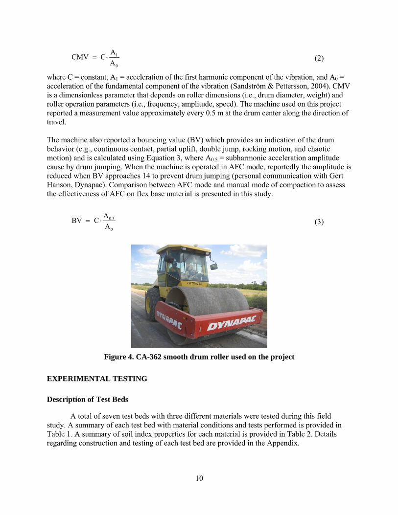
Figure 4. CA-362 smooth drum roller used on the project

EXPERIMENTAL TESTING

Description of Test Beds

A total of seven test beds with three different materials were tested during this field study. A summary of each test bed with material conditions and tests performed is provided in Table 1. A summary of soil index properties for each material is provided in Table 2. Details regarding construction and testing of each test bed are provided in the Appendix.

11

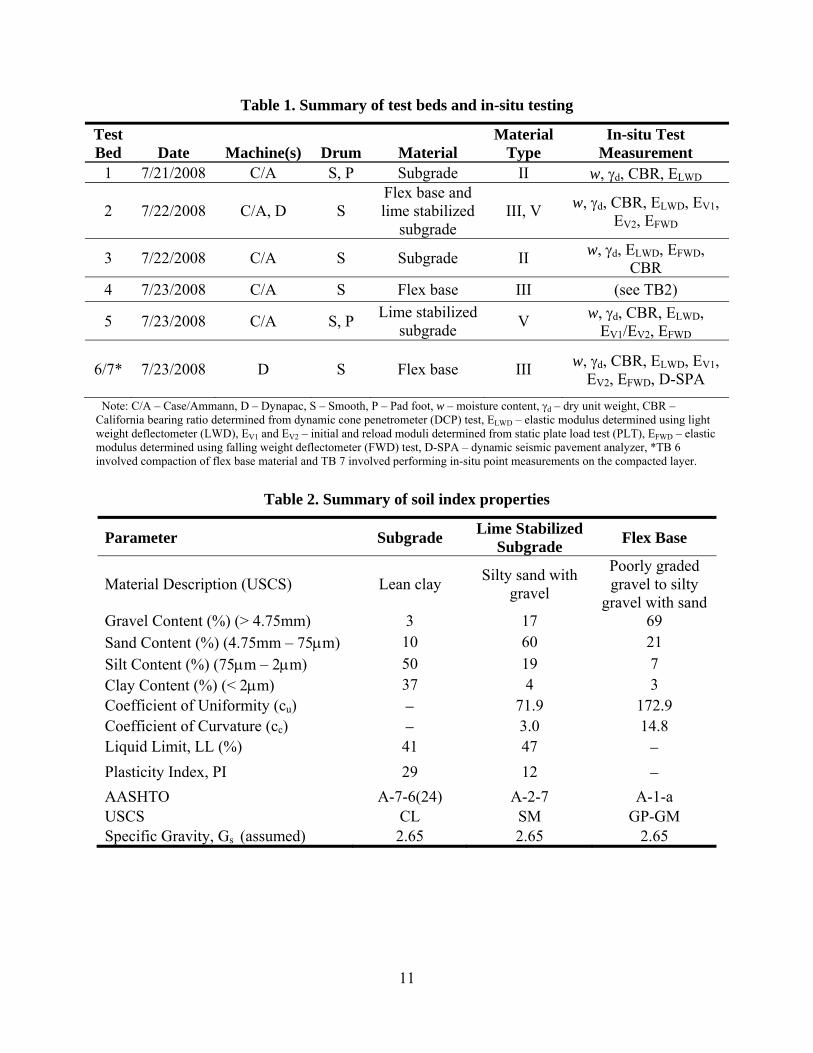
Table 1. Summary of test beds and in-situ testing

Test Bed Date Machine(s) Drum Material

Material Type

In-situ Test Measurement

1 7/21/2008 C/A S, P Subgrade II w, d, CBR, ELWD

2 7/22/2008 C/A, D S Flex base and lime stabilized

subgrade III, V w, d, CBR, ELWD, EV1,

EV2, EFWD

3 7/22/2008 C/A S Subgrade II w, d, ELWD, EFWD, CBR

4 7/23/2008 C/A S Flex base III (see TB2)

5 7/23/2008 C/A S, P Lime stabilized

subgrade V w, d, CBR, ELWD,

EV1/EV2, EFWD

6/7* 7/23/2008 D S Flex base III w, d, CBR, ELWD, EV1, EV2, EFWD, D-SPA

Note: C/A – Case/Ammann, D – Dynapac, S – Smooth, P – Pad foot, w – moisture content, d – dry unit weight, CBR – California bearing ratio determined from dynamic cone penetrometer (DCP) test, ELWD – elastic modulus determined using light weight deflectometer (LWD), EV1 and EV2 – initial and reload moduli determined from static plate load test (PLT), EFWD – elastic modulus determined using falling weight deflectometer (FWD) test, D-SPA – dynamic seismic pavement analyzer, *TB 6 involved compaction of flex base material and TB 7 involved performing in-situ point measurements on the compacted layer.

Table 2. Summary of soil index properties

Parameter Subgrade Lime Stabilized

Subgrade Flex Base

Material Description (USCS) Lean clay Silty sand with

gravel

Poorly graded gravel to silty

gravel with sand Gravel Content (%) (> 4.75mm) 3 17 69 Sand Content (%) (4.75mm – 75m) 10 60 21

Silt Content (%) (75m – 2m) 50 19 7 Clay Content (%) (< 2m) 37 4 3 Coefficient of Uniformity (cu) 71.9 172.9 Coefficient of Curvature (cc) 3.0 14.8 Liquid Limit, LL (%) 41 47

Plasticity Index, PI 29 12 AASHTO A-7-6(24) A-2-7 A-1-a USCS CL SM GP-GM Specific Gravity, Gs (assumed) 2.65 2.65 2.65

12

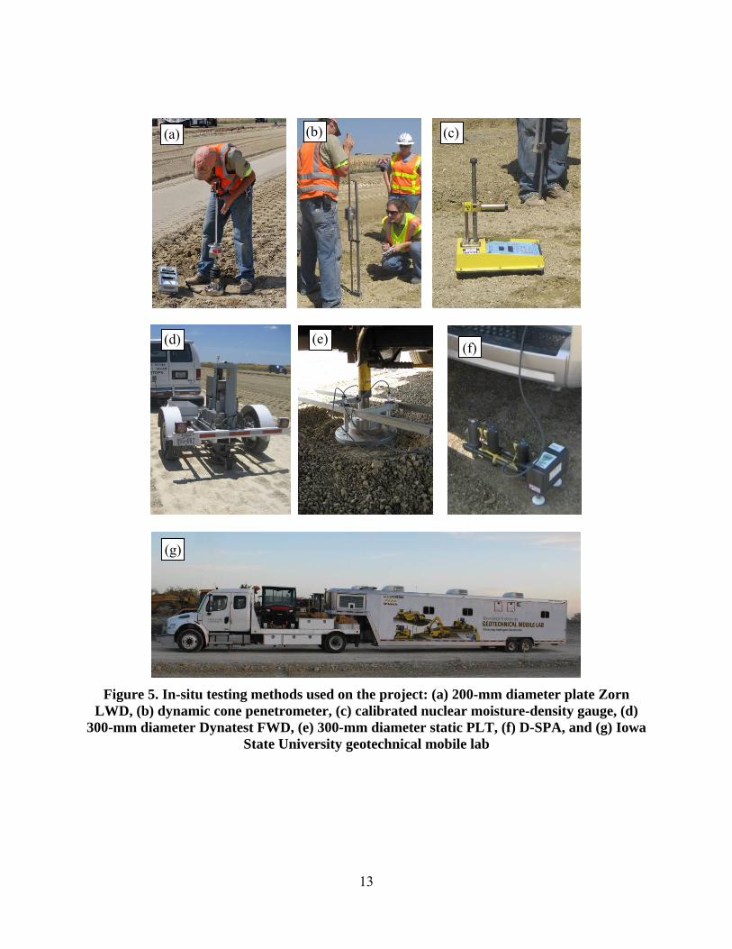
In-situ Testing Methods

Six different in-situ testing methods were employed in this study to evaluate the in-situ soil physical and mechanical properties (Figure 5): (a) 200-mm diameter Zorn LWD setup with 50 mm drop height to determine elastic modulus (ELWD-Z2), (b) Dynamic Cone Penetrometer (DCP) to determine California bearing Ratio (CBR), (c) calibrated nuclear moisture-density gauge (NG), (d) 300-mm diameter Dynatest FWD to determine elastic modulus (EFWD), (e) 300-mm diameter static PLT to determine initial (EV1) and re-load modulus (EV2), and (f) D-SPA to determine low-strain elastic modulus (ED-SPA). LWD, DCP, NG, and PLT tests were conducted by the ISU research team with aid of the geotechnical mobile lab (Figure 5g), FWD tests were conducted by TXDOT personnel (Mr. Robert L. Graham), and D-SPA tests were conducted by University of Texas at El Paso personnel (Prof. Soheil Nazarian and Mr. Deren Yuan). LWD tests were performed following manufacturer recommendations (Zorn 2003) and the ELWD-

Z2 value was determined using Equation 4, where E = elastic modulus (MPa), d0 = measured settlement (mm), v = Poisson’s ratio, 0 = applied stress (MPa), r = radius of the plate (mm), f = shape factor depending on stress distribution (assumed as 8/3 for flex base and/2 for subgrade and lime stabilized subgrade materials). When padfoot roller was used for compaction, the material was carefully excavated down to the bottom of the pad to create a level surface for LWD testing.

20

0

(1 )v rE f

d

(4)

DCP test was performed in accordance with ASTM D6951-03 to determine dynamic cone penetration index (DPI) and calculate CBR using Equation 5. The DCP test results are presented in this report as CBR point values or CBR profiles. When the data is presented as point values, the data represents an average CBR of the compaction layer or the depth specified (e.g., CBR0-250

represents 0-250 mm depth).

1.12

292CBR

DPI (5)

EFWD-D3 values were determined from the stiffness values using Equation 4 (f values were assumed as stated above). Static PLT’s were conducted by applying a static load on 300 mm diameter plate against a 6.2kN capacity reaction force. The applied load was measured using a 90-kN load cell and deformations were measured using three 50-mm linear voltage displacement transducers (LVDTs). The load and deformation readings were continuously recorded during the test using a data logger. The EV1 and EV2 values were determined from Equation 4, using appropriate stress and deflection values as illustrated in Figure 5 depending on the material/layer type. The D-SPA test developed by Nazarian et al. (1993) was used on the project. The resulting modulus values were provided from Transtec.

13

Figure 5. In-situ testing methods used on the project: (a) 200-mm diameter plate Zorn LWD, (b) dynamic cone penetrometer, (c) calibrated nuclear moisture-density gauge, (d)

300-mm diameter Dynatest FWD, (e) 300-mm diameter static PLT, (f) D-SPA, and (g) Iowa State University geotechnical mobile lab

(a) (b) (c)

(d) (e) (f)

(g)

14

0 (MN/m2)

0 (MN/m2)

subgrade base and subbase

0.0

0.1

0.2

0.0

0.2

0.4

Deflection Deflection

EV1 EV2

EV1 EV2

Figure 6. EV1 and EV2 determination procedure from static PLT for subgrade and flex base material

IN-SITU TEST RESULTS AND DISCUSSION

Results and analysis from this field investigation are presented in the following sections. First, brief description of the construction process, and results showing comparison between roller MVs and in-situ point measurements, spatial maps, regression analysis, and conclusions are presented separately for each testbed. Later, comparison measurements obtained between smooth drum and padfoot roller measurements from TBs 1, 3, 4, and 5 are presented. In the end, a general summary and conclusions from this field investigation and recommendations for future work are provided.

TBs 1 and 3 – Clay Subgrade Material

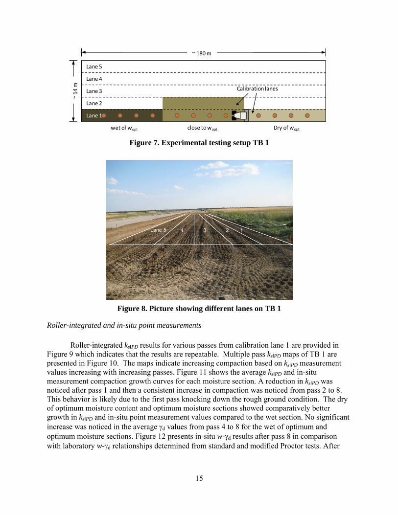
Construction of TBs

TB 1 was constructed by scarifying the existing subgrade material to a depth of about 250

mm. The TB was compacted in five lanes where two lanes were used as calibration test strips and the rest was used for production compaction (see Figure 7 and Figure 8). Lane 1 was prepared with three target moisture sections with moisture contents varying from dry to wet of the materials’ optimum moisture content as shown on Figure 7. Lane 2 was prepared with a target moisture content close to the optimum moisture content (Figure 7). The Case/Ammann pad foot roller was used for compacting the test bed. In-situ point measurements (w, d, CBR, and ELWD-Z2) were obtained after 1, 2, 4, and 8 roller passes in the calibration lanes. Following calibration testing, the test bed was mapped using the padfoot roller. The same area was mapped using the Case/Ammann smooth drum roller (results are identified as TB 3). A few select point locations along Lanes 1 and 5 of TB 3 were also tested to determine EFWD-D3, EV1, w, d, and CBR values, following mapping passes.

Subgrade and lime stabilized subgrade

Flex Base

15

Lane 1

Lane 2

Lane 3

Lane 4

Lane 5

wet of wopt close to wopt Dry of wopt

~ 180 m

~ 14 m Calibration lanes

Figure 7. Experimental testing setup TB 1

Figure 8. Picture showing different lanes on TB 1

Roller-integrated and in-situ point measurements

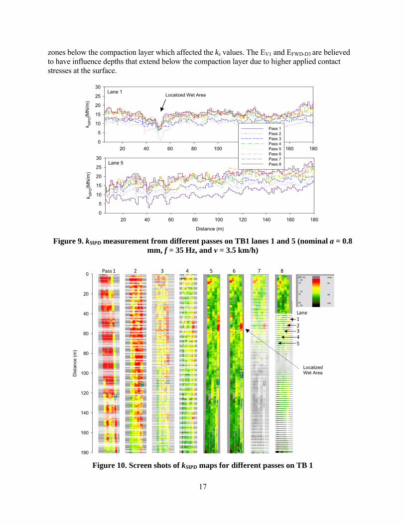
Roller-integrated ksΙPD results for various passes from calibration lane 1 are provided in

Figure 9 which indicates that the results are repeatable. Multiple pass ksΙPD maps of TB 1 are presented in Figure 10. The maps indicate increasing compaction based on ksΙPD measurement values increasing with increasing passes. Figure 11 shows the average ksΙPD and in-situ measurement compaction growth curves for each moisture section. A reduction in ksΙPD was noticed after pass 1 and then a consistent increase in compaction was noticed from pass 2 to 8. This behavior is likely due to the first pass knocking down the rough ground condition. The dry of optimum moisture content and optimum moisture sections showed comparatively better growth in ksΙPD and in-situ point measurement values compared to the wet section. No significant increase was noticed in the average d values from pass 4 to 8 for the wet of optimum and optimum moisture sections. Figure 12 presents in-situ w-d results after pass 8 in comparison with laboratory w-d relationships determined from standard and modified Proctor tests. After

Lane 5 4 3 2 1

16

pass 8, on average the dry of optimum, close to optimum, and wet of optimum sections of the subgrade were at about 96%, 89%, and 88% of the standard Proctor dmax. Comparison between ksΙPD and different in-situ point measurements for calibration lanes 1 and 2 are presented in Figure 13. The ELWD-Z2 point measurements captured the variability observed in the ksΙPD measurements better than the CBR and d measurements. Using the mapping pass measurements from the padfoot (TB 1) and smooth drum rollers (TB3), comparison between ksΙPD, ksΙSD and in-situ point measurements are presented in Figure 14 for lanes 1 and 5. Results show that EFWD-D3 and EV1 measurements tracked well with ks measurement values and the other point measurements showed significant scatter. Simple linear regression relationships between ks and different in-situ point measurements from TBs 1 and 3 are presented in Figure 15 and Figure 16. The relationships were developed by pairing spatially nearest point measurements with the ks data. Spatial locations of point measurements were adjusted up to ± 0.5 m between roller passes to pair with appropriate roller measurement values and involved some judgment. A summary of regression relationships from TBs 1 and 3 are presented in Table 3. The relationships show R2 values ranging from 0 to 0.7. Relationships with EFWD and EV1 measurements produced comparatively higher correlations with R2 > 0.6. To further assess scatter observed in the regressions, full depth CBR profiles from TB 1 were analyzed as shown in Figure 17 and Figure 18. CBR values for the underlying subgrade layer were determined (average CBR from 250 to 500 mm depth) and compared with the ks values. This comparison indicates that in the dry of optimum portion of calibration lane 1 (i.e., position 120 m to 180 m) where the compaction layer CBR > 13, the ks values are better correlated with the underlying layer CBR values. In the wet of optimum portion (i.e., position 0 to 60 m) where the compaction layer CBR < 8 the ks values are better correlated with the compaction layer CBR values. This finding suggests that the roller-integrated ks values are influenced by “soft” zones in the compaction layer as well as below the compaction layer. The d, CBR, and ELWD-Z2 measurements represent only the compaction layer (i.e., within 250 mm depth) properties and therefore did not match well with ks measurements which were influenced by the underlying “soft” layers. The EV1 and EFWD-D3 measurements are believed to have greater influence depths due to larger plate diameter (300 mm) and higher applied contact stresses. Therefore, the EV1 and EFWD-D3

produced better correlations with the ks values. Relating full depth (up to 1m) DCP-CBR profile information to correlate with ks values is a topic of ongoing research for the research team.

Summary

Both padfoot and smooth drum roller-integrated ks values (ksΙPD and ksΙSD) reliably indicate the compaction quality of the subgrade clay material with good repeatability. Regression relationships between ks and different in-situ point measurements show positive correlations with varying degree of uncertainty in the correlations (as assessed by the R2 values), however. Correlations with EFWD

and EV1 values (with R2 > 0.6) produced better R2 values compared to ELWD-Z2, d, and CBR (of the compaction layer) measurements. Poorer correlations with ELWD-Z2, d, and CBR compaction layer values is attributed to the limitation of shallow measurement influence depth of these measurements (≤ 250 mm). CBR profiles up to 1 m generated from DCP tests identified “soft”

17

zones below the compaction layer which affected the ks values. The EV1 and EFWD-D3 are believed to have influence depths that extend below the compaction layer due to higher applied contact stresses at the surface.

Distance (m)

20 40 60 80 100 120 140 160 180

k SIP

D(M

N/m

)

0

5

10

15

20

25

30

20 40 60 80 100 120 140 160 180

k SIP

D(M

N/m

)

0

5

10

15

20

25

30

Pass 1Pass 2Pass 3Pass 4Pass 5Pass 6Pass 7Pass 8

Lane 1

Lane 5

Figure 9. kSΙPD measurement from different passes on TB1 lanes 1 and 5 (nominal a = 0.8 mm, f = 35 Hz, and v = 3.5 km/h)

Dis

tanc

e (m

)

0

20

40

60

80

100

120

140

160

180

Pass 1 2 3 4 5 6 7 8

Lane12345

Figure 10. Screen shots of kSΙPD maps for different passes on TB 1

Localized Wet Area

Localized Wet Area

18

Pass

0 2 4 6 8 10

Ave

rage

ELW

D-Z

2 (M

Pa)

6

9

12

15

18

Pass

0 2 4 6 8 10

Ave

rage

d

(kN

/m3)

13

14

15

16

17

18

19

Section 1 - Dry Section 2 - OptimumSection 3 - Wet

0 2 4 6 8 10

Ave

rage

w (

%)

5

10

15

20

25

30

35

Pass

0 2 4 6 8 10

Ave

rage

CB

R (

%)

3

6

9

12

15

18

0 2 4 6 8 10

Ave

rag

e k S

IPD (

MN

/m)

8

10

12

14

16

18

20

Std. Proctor wopt = 17.8%

Std. Proctor dmax = 16.8 kN/m3

Figure 11. Compaction growth curves for kSΙPD and in-situ point measurements (TB 1 lane 1 calibration test strip, nominal a = 0.8 mm, f = 35 Hz, and v = 3.5 km/h)

Moisture Content, w (%)

0 5 10 15 20 25

Dry

Uni

t W

eig

ht, d

(kN

/m3)

14

16

18

20Standard PrctorModified ProctorIn-situ w-d, Pass 8

Gs = 2.70

ZAV line

Figure 12. Comparison of laboratory Proctor curves and in-situ w-d measurements after pass 8 – TB 1 subgrade material

Initial pass over rough grade

19

40 80 120 160

k SIP

D(M

N/m

)

0

10

20

30

40 80 120 160

ELW

D-Z

2(M

Pa)

0

10

20

30

40 80 120 160

k SIP

D(M

N/m

)

0

10

20

30

40 80 120 160

ELW

D-Z

2(M

Pa)

0

10

20

30

40 80 120 160

k SIP

D(M

N/m

)

0

10

20

30

40 80 120 160E

LWD

-Z2(

MP

a)

0

10

20

30

40 80 120 160

k SIP

D(M

N/m

)

0

10

20

30

40 80 120 160

ELW

D-Z

2(M

Pa)

0

10

20

30

Lane 1 Lane 2Pass 1

Pass 2

Pass 4

Pass 8

40 80 120 160

k SIP

D(M

N/m

)

0

10

20

30

40 80 120 160

CB

R (

%)

0

5

10

15

20

40 80 120 160

k SIP

D(M

N/m

)

0

10

20

30

40 80 120 160

CB

R (

%)

0

5

10

15

20

40 80 120 160

k SIP

D(M

N/m

)

0

10

20

30

40 80 120 160

CB

R (

%)

0

5

10

15

20

40 80 120 160

k SIP

D(M

N/m

)

0

10

20

30

40 80 120 160

CB

R (

%)

0

5

10

15

20

Lane 1 Lane 2Pass 1

Pass 2

Pass 4

Pass 8

40 80 120 160

k SIP

D(M

N/m

)

0

10

20

30

40 80 120 160

w (

%)

0

10

20

30

40

40 80 120 160

k SIP

D(M

N/m

)

0

10

20

30

40 80 120 160

w (

%)

0

10

20

30

40

40 80 120 160

k SIP

D(M

N/m

)

0

10

20

30

40 80 120 160

w (

%)

0

10

20

30

40

Distance (m)

40 80 120 160

k SIP

D(M

N/m

)

0

10

20

30

40 80 120 160

w (

%)

0

10

20

30

40

Lane 1 Lane 2Pass 1

Pass 2

Pass 4

Pass 8

40 80 120 160

k SIP

D(M

N/m

)

0

10

20

30

40 80 120 160

d (

kN/m

3 )

12

15

18

40 80 120 160

k SIP

D(M

N/m

)

0

10

20

30

40 80 120 160 d

(kN

/m3 )

12

15

18

40 80 120 160

k SIP

D(M

N/m

)

0

10

20

30

40 80 120 160

d (

kN/m

3 )

12

15

18

40 80 120 160

k SIP

D(M

N/m

)

0

10

20

30

40 80 120 160

d (

kN/m

3)

12

15

18

Lane 1 Lane 2Pass 1

Pass 2

Pass 4

Pass 8

Distance (m)

Figure 13. Comparison between kSΙPD and in-situ point measurements at passes 1, 2, 4, and 8 (TB 1 lane 1, nominal a = 0.8 mm, f = 35 Hz, and v = 3.5 km/h)

20

40 80 120 160

k s (M

N/m

)

0

10

20

30

40 80 120 160

w (

%)

0

5

10

15

20

Lane 1 Lane 5

40 80 120 160

k s (M

N/m

)

0

10

20

30

40 80 120 160

d (

kN/m

3)

12

15

18

21

40 80 120 160

k s (M

N/m

)

0

10

20

30

40 80 120 160

EL

WD

-Z2(M

Pa)

0

20

40

60

80

40 80 120 160

k s (M

N/m

)

0

10

20

30

40 80 120 160

CB

R (

%)

0

10

20

30

40 80 120 160

k s (M

N/m

)

0

10

20

30

40 80 120 160

EF

WD

-D3(M

Pa)

020406080100

Dist 1-lane 1 vs ks Pass 1 Dist 1-lane 1 vs ks Pass 1 Dist 1-lane 1 vs ks Pass 1 Dist 1-lane 1 vs ks Pass 1 Dist 1-lane 1 vs ks Pass 1 Dist 1-lane 1 vs ks Pass 1 Dist 1-lane 1 vs ks Pass 1 Dist 1-lane 1 vs ks Pass 1

40 80 120 160k s

(MN

/m)

0

10

20

30

40 80 120 160

EV

1(M

Pa)

01020304050

kSIPD

kSISD

Lane 1 Lane 5

Figure 14. Comparison between kSΙPD, kSΙSD, and in-situ point measurements from TB3 (kSΙSD: mapping pass, a = 1.1 mm, f = 30 Hz, v = 3.5 km/h; kSΙPD: pass 8, a = 0.8 mm, f = 35

Hz, v = 3.5 km/h)

Table 3. Summary of simple linear regression analysis – TBs 1 and 3

TB Settings Drum Model*

n b0 b1 R2

1/3 a = 0.8 mm f = 35 Hz

Padfoot

kSIPD = b0 + b1 ELWD-Z2 120 11.60 0.17 0.29 kSIPD = b0 + b1 d 75 -14.50 1.92 0.33 kSIPD = b0 + b1 CBR 81 10.69 0.43 0.40 kSIPD = b0 + b1 EV1 18 8.51 0.49 0.72 kSIPD = b0 + b1 EV2 18 11.20 0.16 0.50 kSIPD = b0 + b1 EFWD-D3 53 6.38 0.25 0.63 kSIPD = b0 + b1 ED-SPA 48 7.20 0.03 0.47

1/3 a = 1.1 mm f = 30 Hz

Smooth

kSISD = b0 + b1 ELWD-Z2 56 7.86 0.10 0.10 kSISD = b0 + b1 d 12 NS†

kSISD = b0 + b1 CBR 17 5.44 0.39 0.37 kSISD = b0 + b1 EV1 18 -4.16 0.79 0.67 kSISD = b0 + b1 EV2 18 -0.32 0.27 0.45 kSISD = b0 + b1 EFWD-D3 53 -2.78 0.33 0.75 kSISD = b0 + b1 ED-SPA 48 1.78 0.03 0.29

*Units: ks (MN/m), d (kN/m3), CBR (%), ELWD-Z2/EV1/EV2/EFWD-D3/ED-SPA (MPa). † NS – not statistically significant according to p < 0.10 and t < -2 or > +2.

21

d (kN/m3)

5 10 15 20 25 30

k SIP

D(M

N/m

)

0

5

10

15

20

25

30

EV2 (MPa)

20 40 60 80 1000

5

10

15

20

25

30

ELWD-Z2 (MPa)

0 20 40 60

k SIP

D(M

N/m

)

0

5

10

15

20

25

30

CBR (%)

0 5 10 15 200

5

10

15

20

25

30

d (kN/m3)

12 13 14 15 16 17 180

5

10

15

20

25

30

R2 = 0.30n = 120

R2 = 0.40n = 81

R2 = 0.33n = 75

EV1 (MPa)

10 15 20 25 30 35 400

5

10

15

20

25

30

EFWD-D3 (MPa)

10 20 30 40 50 60 70

k SIP

D(M

N/m

)

0

5

10

15

20

25

30

ED-SPA (MPa)

100 200 300 400 5000

5

10

15

20

25

30

R2 = 0.12n = 75

R2 = 0.72n = 18

R2 = 0.50n = 18

R2 = 0.63n = 53

R2 = 0.48n = 48

Figure 15. Simple linear regression relationships between kSΙPD and in-situ point measurements (TB 1 – subgrade clay material, nominal a = 0.8 mm, f = 35 Hz, and v = 3.2

km/h)

22

w

10 11 12 13 14 15 16 17

k SIS

D(M

N/m

)

0

5

10

15

20

25

30

EV2 (MPa)

20 40 60 80 1000

5

10

15

20

25

30

ELWD-Z2 (MPa)

0 20 40 60

k SIS

D(M

N/m

)

0

5

10

15

20

25

30

CBR (%)

0 5 10 15 200

5

10

15

20

25

30

d (kN/m3)

12 13 14 15 16 17 180

5

10

15

20

25

30R2 = 0.10n = 56

EV1 (MPa)

10 15 20 25 30 35 400

5

10

15

20

25

30

EFWD-D3 (MPa)

10 20 30 40 50 60 70

k SIS

D(M

N/m

)

0

5

10

15

20

25

30

ED-SPA (MPa)

100 200 300 400 5000

5

10

15

20

25

30

R2 = 0.37n = 17 n = 12

R2 = 0.16n = 12

R2 = 0.67n = 18

R2 = 0.45n = 18

R2 = 0.75n = 53

R2 = 0.29n = 48

Figure 16. Simple linear regression relationships between kSΙSD and in-situ point measurements (TB 1 – subgrade clay material, nominal a = 1.1 mm, f = 30 Hz, and v = 3.5

km/h)

23

CBR (%)

0 5 10 15 20 25 30

0

200

400

600

800

CBR (%)

0 5 10 15 20 25 30

0

200

400

600

800

CBR (%)

0 5 10 15 20 25 30

Dep

th (

mm

)

0

200

400

600

800

Pass 1Pass 2Pass 4Pass 8

CBR (%)

0 5 10 15 20 25 30

0

200

400

600

800

Distance (m)

120 125 130 135 140 145 150 155 160 165 170 175 180

k SIP

D(M

N/m

)

0

10

20

30

CB

R0-

250

(%)

0

5

10

15

20

CB

R25

0-50

0 (%

)

0

5

10

15

ks

CBR0-250

CBR250-500

Pass 8Lane 1 (Average w = 12.1%)

Distance (m)

60 65 70 75 80 85 90 95 100 105 110 115 120

k SIP

D(M

N/m

)

0

10

20

30

CB

R0-

250

(%)

0

5

10

15

20

CB

R25

0-50

0 (%

)

0

5

10

15ks

CBR0-250

CBR250-500

Pass 8Lane 1 (Average w = 18.8%)

(4)(3)

(2)

(1)

(4) (3) (2) (1)

(8) (7)

(6) (5)

CBR (%)

0 5 10 15 20 25 30

0

200

400

600

800(5)

CBR (%)

0 5 10 15 20 25 30

0

200

400

600

800(6)

CBR (%)

0 5 10 15 20 25 30

0

200

400

600

800(7)

CBR (%)

0 5 10 15 20 25 30

Dep

th (

mm

)

0

200

400

600

800

Pass 1Pass 2Pass 4Pass 8

(8)

Figure 17. Comparison between roller MV and CBR profiles from TB 1 – lane 1 between 60 to 180 m (pass 8, nominal a = 0.8 mm, f = 35 Hz, and v = 3.5 km/h)

24

Distance (m)

0 5 10 15 20 25 30 35 40 45 50 55 60

k SIP

D(M

N/m

)

0

10

20

30

CB

R0-

250(

%)

0

5

10

15

20

CB

R25

0-50

0(%

)

0

5

10

15ks

CBR0-250

CBR250-500

Pass 8Lane 1 (Average w = 21.7%)

(12) (11) (10)(9)

Distance (m)

60 65 70 75 80 85 90 95 100 105 110 115 120

k SIP

D(M

N/m

)

0

10

20

30

CB

R0-

250(

%)

0

5

10

15

20

CB

R25

0-50

0(%

)

0

5

10

15

ks

CBR0-250

CBR250-500Pass 8Lane 2 (Average w = 19.9%)

CBR (%)

0 5 10 15 20 25 30

0

200

400

600

800

CBR (%)

0 5 10 15 20 25 30

0

200

400

600

800

CBR (%)

0 5 10 15 20 25 30

0

200

400

600

800

Pass 1Pass 2Pass 4Pass 8

CBR (%)

0 5 10 15 20 25 30

Dep

th (

mm

)

0

200

400

600

800 (16) (15) (14) (13)

(16) (15)(14)

(13)

CBR (%)

0 5 10 15 20 25 30

Dep

th (

mm

)

0

200

400

600

800(12)

CBR (%)

0 5 10 15 20 25 30

0

200

400

600

800(11)

CBR (%)

0 5 10 15 20 25 30

0

200

400

600

800(10)

CBR (%)

0 5 10 15 20 25 30

0

200

400

600

800(9)

Figure 18. Comparison between roller MV and CBR profiles from TB 1 – lane 1 between 0 and 60 m, and lane 2 between 60 and 120 m (pass 8, nominal a = 0.8 mm, f = 35 Hz, v = and

3.5 km/h)

25

TB 2 lime-stabilized subgrade and flex base material

Construction and testing on TB2

TB 2 consisted of a compacted layer of lime stabilized subgrade material transitioning to

flex base at each end of the TB (Figure 19). The flex base layer was significantly stiffer than the stabilized subgrade material and provided a field condition to evaluate the ability of the roller to distinguish between different ground conditions. Case/Ammann and Dynapac smooth drum rollers were used for mapping the TB with different amplitude settings (Figure 20). Following mapping passes, in-situ point measurements (w, d, CBR, ELWD-Z2, EFWD-D3, and ED-SPA) were obtained from lane 2 of the test bed (see Figure 20).

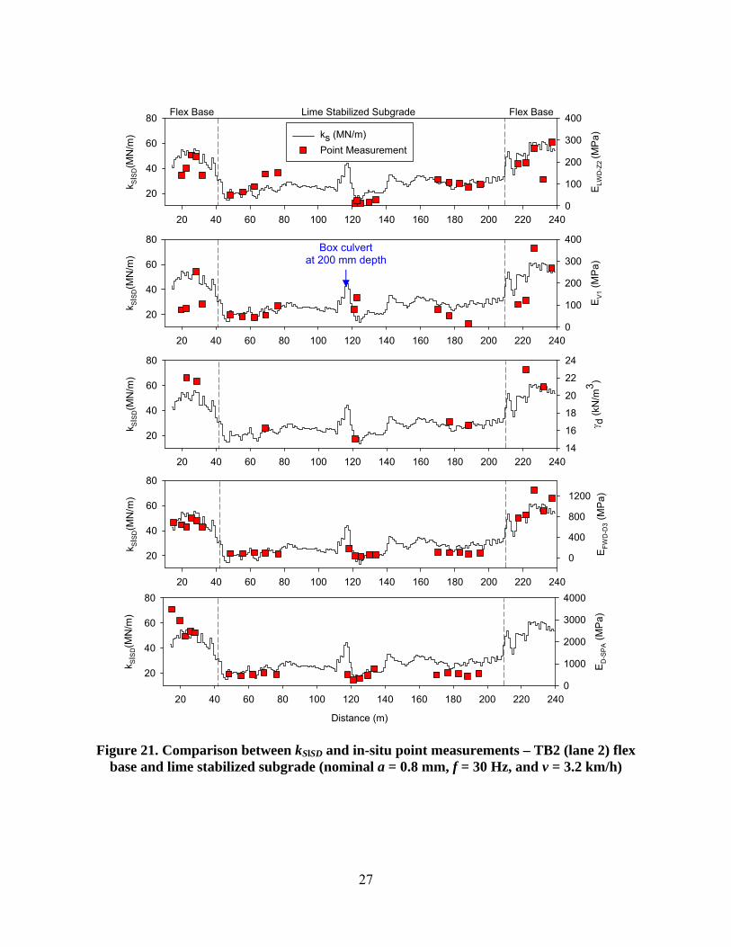
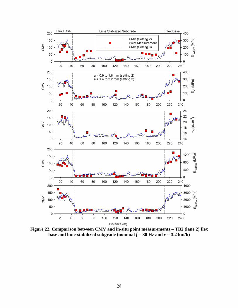
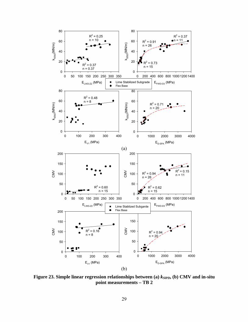
Roller-integrated and in-situ point measurements

Spatial maps of roller-integrated kSΙSD and CMV (from two different amplitude settings)

are presented in Figure 20. Comparison results from lane 2 between CMV, kSΙSD and in-situ point measurements are presented in Figure 21 and Figure 22. Results indicate that the wide variation in stiffness of the two materials in the test bed were well-captured by the in-situ point measurements and the two roller MVs. A box culvert located at a location within the lime stabilized subgrade portion of the test bed was well captured by the roller MVs (see Figure 21 and Figure 22). CMV measurements at the two amplitude settings were similar and reproducible (see Figure 22). Regression relationships based on spatially paired nearest point data are presented in Figure 23, and the relationships are summarized in Table 4. Results generally show separate linear trends for the lime stabilized and flex base materials. Linear regression analysis indicates comparatively better correlations with EFWD measurements than with other point measurements. Hyperbolic regression relationships are provided for EFWD and ED-SPA measurements combining measurements on flex base and lime stabilized subgrade materials. These relationships are presented only to demonstrate the trends, however, additional data is needed especially for CMV between 50 and 100, and ks between 30 and 50 to validate the relationships.

Summary

Both roller MVs and in-situ point measurements captured the wide variation in stiffness

of the compacted lime stabilized and flex base materials. A box-culvert located beneath the lime stabilized subgrade was identified with high roller MVs in that location. Linear regression relationships generally indicate separate linear trends for the lime stabilized and flex base materials. EFWD measurements produced better correlations than other point measurements. Hyperbolic regression relationships were developed for EFWD and ED-SPA measurements which showed strong correlations with ks and CMV measurements but additional data is needed to validate the relationships. The CMV measurements at this location were highly repeatable.

26

Figure 19. Picture of TB2 with flex base (on both ends of the test bed) and lime stabilized subgrade

Figure 20. Comparison between kSΙSD CMV maps– TB2 flex base and lime-stabilized subgrade

Lane 2 

Lane 2 

Lane 2    

CMV Map a = 1.9 mm, f = 30 Hz, v = 3.5 km/h 

CMV Map a = 1.2 mm, f = 30 Hz, v = 3.5 km/h 

kSΙSD Map a = 0.8 mm, f = 30 Hz, and v = 3.2 km/h 

Flex Base

Lime Stabilized Subgrade

Flex Base

Flex Base Flex Base Lime stabilized subgrade

27

20 40 60 80 100 120 140 160 180 200 220 240

k SIS

D(M

N/m

)

20

40

60

80

EL

WD

-Z2

(MP

a)

0

100

200

300

400

ks (MN/m)

Point Measurement

20 40 60 80 100 120 140 160 180 200 220 240

k SIS

D(M

N/m

)

20

40

60

80

EV

1 (

MP

a)

0

100

200

300

400

20 40 60 80 100 120 140 160 180 200 220 240

k SIS

D(M

N/m

)

20

40

60

80

d (

kN/m

3)

14

16

18

20

22

24

20 40 60 80 100 120 140 160 180 200 220 240

k SIS

D(M

N/m

)

20

40

60

80

EF

WD

-D3 (

MP

a)

0

400

800

1200

Flex Base Flex BaseLime Stabilized Subgrade

Distance (m)

20 40 60 80 100 120 140 160 180 200 220 240

k SIS

D(M

N/m

)

20

40

60

80E

D-S

PA (

MP

a)

0

1000

2000

3000

4000

Figure 21. Comparison between kSΙSD and in-situ point measurements – TB2 (lane 2) flex base and lime stabilized subgrade (nominal a = 0.8 mm, f = 30 Hz, and v = 3.2 km/h)

Box culvert at 200 mm depth

28

20 40 60 80 100 120 140 160 180 200 220 240

CM

V

0

50

100

150

200

EL

WD

-Z2 (

MP

a)

0

100

200

300

400

CMV (Setting 2)Point MeasurementCMV (Setting 3)

20 40 60 80 100 120 140 160 180 200 220 240

CM

V

0

50

100

150

200

EV

1 (

MP

a)

0

100

200

300

400

20 40 60 80 100 120 140 160 180 200 220 240

CM

V

0

50

100

150

200

d (

kN/m

3)

14

16

18

20

22

24

20 40 60 80 100 120 140 160 180 200 220 240

CM

V

0

50

100

150

200

EF

WD

-D3 (

MP

a)

0

400

800

1200

a = 0.9 to 1.6 mm (setting 2)a = 1.4 to 2.2 mm (setting 3)

Flex Base Flex BaseLime Stabilized Subgrade

Distance (m)

20 40 60 80 100 120 140 160 180 200 220 240

CM

V

0

50

100

150

200

ED

-SP

A (

MP

a)

0

1000

2000

3000

4000

Figure 22. Comparison between CMV and in-situ point measurements – TB2 (lane 2) flex

base and lime-stabilized subgrade (nominal f = 30 Hz and v = 3.2 km/h)

29

EV1 (MPa)

0 100 200 300 400

k SIS

D(M

N/m

)

0

20

40

60

80

ELWD-Z2 (MPa)

0 50 100 150 200 250 300 350

k SIS

D(M

N/m

)

0

20

40

60

80

EFWD-D3 (MPa)

0 200 400 600 800 100012001400

k SIS

D(M

N/m

)

0

20

40

60

80

ED-SPA (MPa)

0 1000 2000 3000 4000

k SIS

D(M

N/m

)

0

20

40

60

80

Lime Stabilized SubgradeFlex Base

R2 = 0.37 n = 0.37

R2 = 0.37n = 11

R2 = 0.48n = 8

R2 = 0.25 n = 10

R2 = 0.73n = 15

R2 = 0.91n = 26

R2 = 0.71n = 20

(a)

EV1 (MPa)

0 100 200 300 400

CM

V

0

50

100

150

200

ELWD-Z2 (MPa)

0 50 100 150 200 250 300 350

CM

V

0

50

100

150

200

EFWD-D3 (MPa)

0 200 400 600 800 100012001400

CM

V

0

50

100

150

200

ED-SPA (MPa)

0 1000 2000 3000 4000

CM

V

0

50

100

150

200

Lime Stablized SubgardeFlex Base

R2 = 0.60n = 15

R2 = 0.15n = 11

R2 = 0.16n = 8

R2 = 0.62n = 15

R2 = 0.94n = 26

R2 = 0.94n = 20

(b)

Figure 23. Simple linear regression relationships between (a) kSΙPD, (b) CMV and in-situ point measurements – TB 2

30

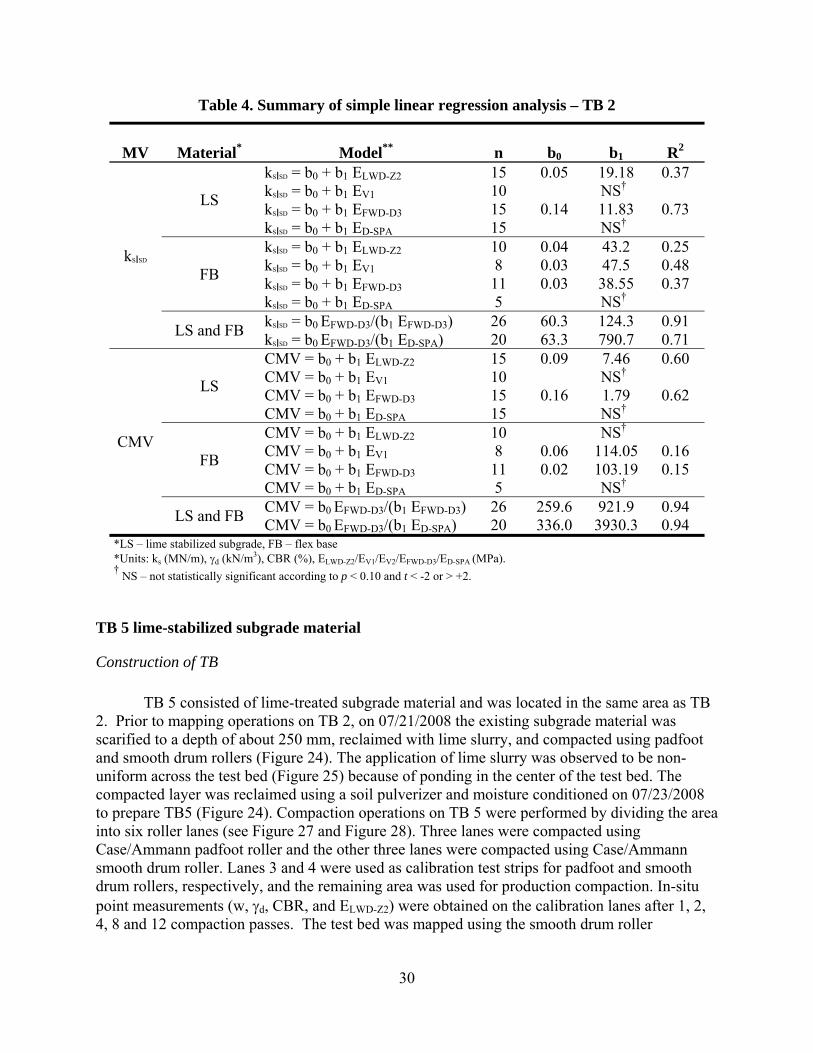
Table 4. Summary of simple linear regression analysis – TB 2

MV Material* Model**

n b0 b1 R2

kSISD

LS

kSISD = b0 + b1 ELWD-Z2 15 0.05 19.18 0.37 kSISD = b0 + b1 EV1 10 NS† kSISD = b0 + b1 EFWD-D3 15 0.14 11.83 0.73 kSISD = b0 + b1 ED-SPA 15 NS†

FB

kSISD = b0 + b1 ELWD-Z2 10 0.04 43.2 0.25 kSISD = b0 + b1 EV1 8 0.03 47.5 0.48 kSISD = b0 + b1 EFWD-D3 11 0.03 38.55 0.37 kSISD = b0 + b1 ED-SPA 5 NS†

LS and FB kSISD = b0 EFWD-D3/(b1 EFWD-D3) 26 60.3 124.3 0.91 kSISD = b0 EFWD-D3/(b1 ED-SPA) 20 63.3 790.7 0.71

CMV

LS

CMV = b0 + b1 ELWD-Z2 15 0.09 7.46 0.60 CMV = b0 + b1 EV1 10 NS† CMV = b0 + b1 EFWD-D3 15 0.16 1.79 0.62 CMV = b0 + b1 ED-SPA 15 NS†

FB

CMV = b0 + b1 ELWD-Z2 10 NS† CMV = b0 + b1 EV1 8 0.06 114.05 0.16 CMV = b0 + b1 EFWD-D3 11 0.02 103.19 0.15 CMV = b0 + b1 ED-SPA 5 NS†

LS and FB CMV = b0 EFWD-D3/(b1 EFWD-D3) 26 259.6 921.9 0.94 CMV = b0 EFWD-D3/(b1 ED-SPA) 20 336.0 3930.3 0.94

*LS – lime stabilized subgrade, FB – flex base *Units: ks (MN/m), d (kN/m3), CBR (%), ELWD-Z2/EV1/EV2/EFWD-D3/ED-SPA (MPa). † NS – not statistically significant according to p < 0.10 and t < -2 or > +2.

TB 5 lime-stabilized subgrade material

Construction of TB

TB 5 consisted of lime-treated subgrade material and was located in the same area as TB

2. Prior to mapping operations on TB 2, on 07/21/2008 the existing subgrade material was scarified to a depth of about 250 mm, reclaimed with lime slurry, and compacted using padfoot and smooth drum rollers (Figure 24). The application of lime slurry was observed to be non-uniform across the test bed (Figure 25) because of ponding in the center of the test bed. The compacted layer was reclaimed using a soil pulverizer and moisture conditioned on 07/23/2008 to prepare TB5 (Figure 24). Compaction operations on TB 5 were performed by dividing the area into six roller lanes (see Figure 27 and Figure 28). Three lanes were compacted using Case/Ammann padfoot roller and the other three lanes were compacted using Case/Ammann smooth drum roller. Lanes 3 and 4 were used as calibration test strips for padfoot and smooth drum rollers, respectively, and the remaining area was used for production compaction. In-situ point measurements (w, d, CBR, and ELWD-Z2) were obtained on the calibration lanes after 1, 2, 4, 8 and 12 compaction passes. The test bed was mapped using the smooth drum roller

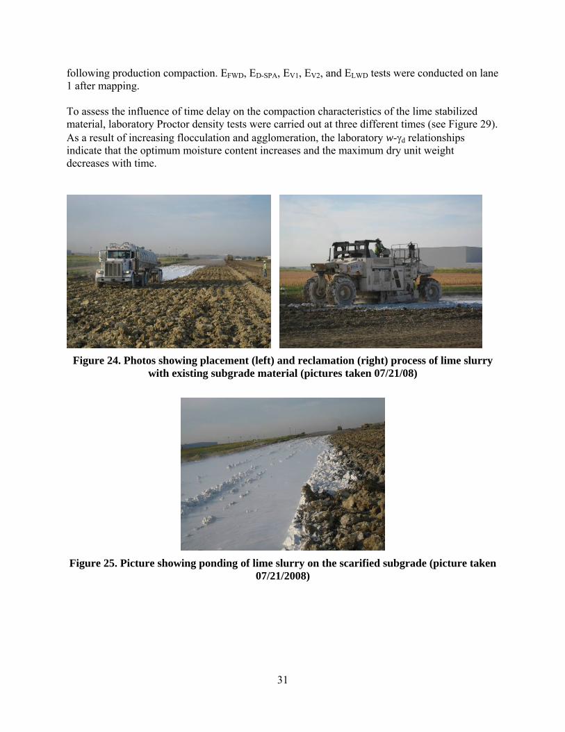
31

following production compaction. EFWD, ED-SPA, EV1, EV2, and ELWD tests were conducted on lane 1 after mapping.

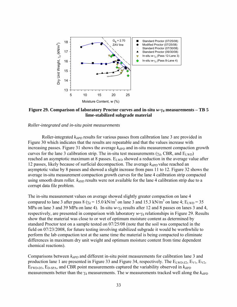
To assess the influence of time delay on the compaction characteristics of the lime stabilized material, laboratory Proctor density tests were carried out at three different times (see Figure 29). As a result of increasing flocculation and agglomeration, the laboratory w-d relationships indicate that the optimum moisture content increases and the maximum dry unit weight decreases with time.

Figure 24. Photos showing placement (left) and reclamation (right) process of lime slurry with existing subgrade material (pictures taken 07/21/08)

Figure 25. Picture showing ponding of lime slurry on the scarified subgrade (picture taken 07/21/2008)

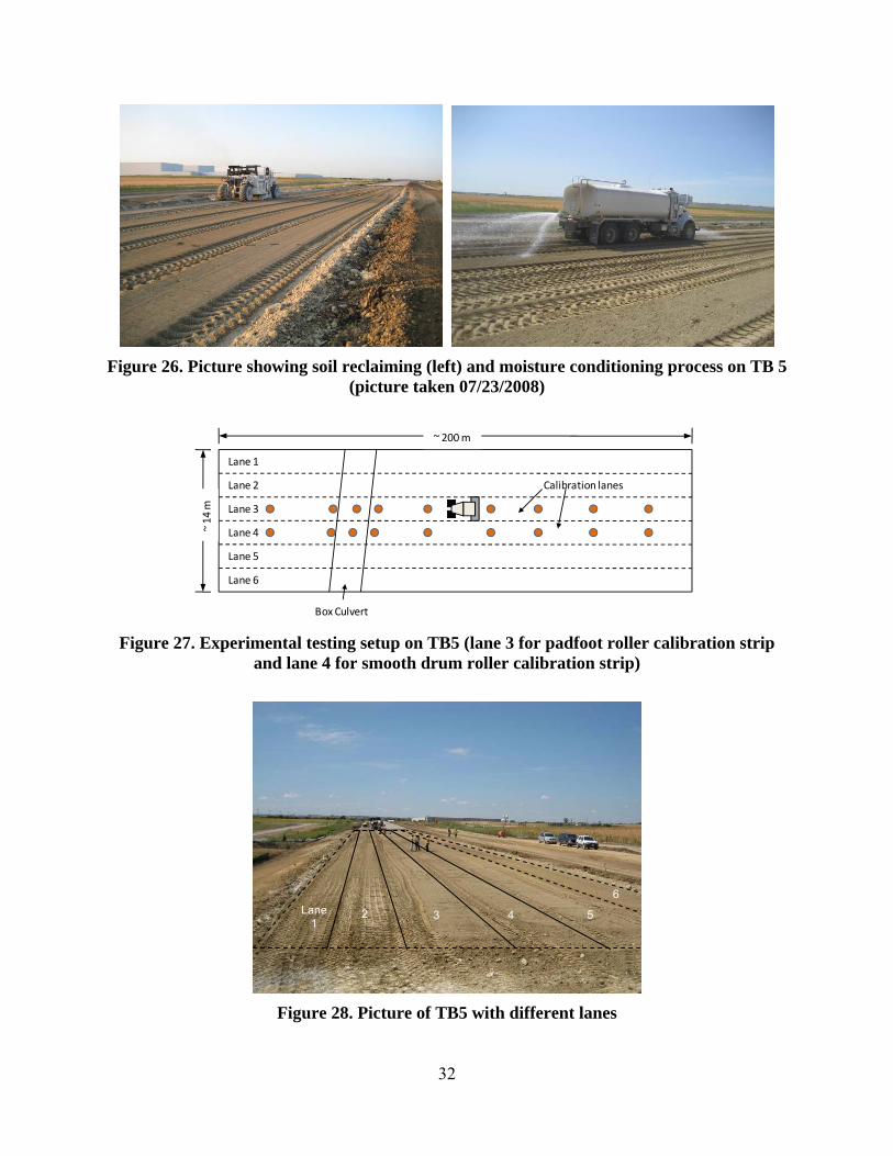
32

Figure 26. Picture showing soil reclaiming (left) and moisture conditioning process on TB 5 (picture taken 07/23/2008)

Lane 6

Lane 5

Lane 4

Lane 3

Lane 2

~ 200 m

~ 14 m

Calibration lanes

Lane 1

Box Culvert

Figure 27. Experimental testing setup on TB5 (lane 3 for padfoot roller calibration strip and lane 4 for smooth drum roller calibration strip)

Figure 28. Picture of TB5 with different lanes

Lane 1

2 3 4 5

6

33

Moisture Content, w (%)

5 10 15 20 25

Dry

Un

it W

eigh

t,

d (

kN/m

3 )

13

14

15

16

17

18 Standard Proctor (07/25/08)Modified Proctor (07/25/08)Standard Proctor (07/30/08)Standard Proctor (09/30/08)In-situ w-d (Pass 12-Lane 3)

In-situ w-d (Pass 8-Lane 4)

Gs = 2.70

ZAV line

Figure 29. Comparison of laboratory Proctor curves and in-situ w-d measurements – TB 5 lime-stabilized subgrade material

Roller-integrated and in-situ point measurements

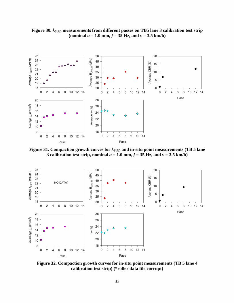
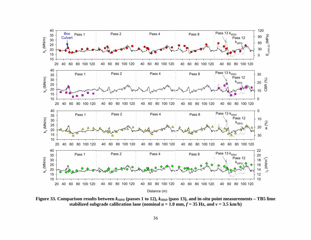
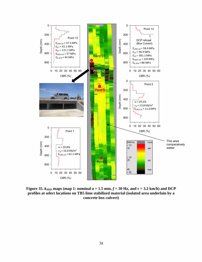
Roller-integrated ksΙPD results for various passes from calibration lane 3 are provided in

Figure 30 which indicates that the results are repeatable and that the values increase with increasing passes. Figure 31 shows the average ksΙPD and in-situ measurement compaction growth curves for the lane 3 calibration strip. The in-situ test measurements (d, CBR, and ELWD) reached an asymptotic maximum at 8 passes. ELWD showed a reduction in the average value after 12 passes, likely because of surficial decompaction. The average ksΙPD value reached an asymptotic value by 8 passes and showed a slight increase from pass 11 to 12. Figure 32 shows the average in-situ measurement compaction growth curves for the lane 4 calibration strip compacted using smooth drum roller. ksΙSD results were not available for the lane 4 calibration strip due to a corrupt data file problem. The in-situ measurement values on average showed slightly greater compaction on lane 4 compared to lane 3 after pass 8 (d = 15.0 kN/m3 on lane 3 and 15.3 kN/m3 on lane 4; ELWD = 35 MPa on lane 3 and 39 MPa on lane 4). In-situ w-d results after 12 and 8 passes on lanes 3 and 4, respectively, are presented in comparison with laboratory w-d relationships in Figure 29. Results show that the material was close to or wet of optimum moisture content as determined by standard Proctor test on a sample tested on 07/25/08 (note that the soil was compacted in the field on 07/23/2008, for future testing involving stabilized subgrade it would be worthwhile to perform the lab compaction test at the same time the material is being compacted to eliminate differences in maximum dry unit weight and optimum moisture content from time dependent chemical reactions).

Comparisons between ksΙPD and different in-situ point measurements for calibration lane 3 and production lane 1 are presented in Figure 33 and Figure 34, respectively. The ELWD-Z2, EV1, EV2, EFWD-D3, ED-SPA, and CBR point measurements captured the variability observed in ksΙPD measurements better than the d measurements. The w measurements tracked well along the ksΙPD

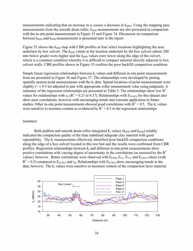
34

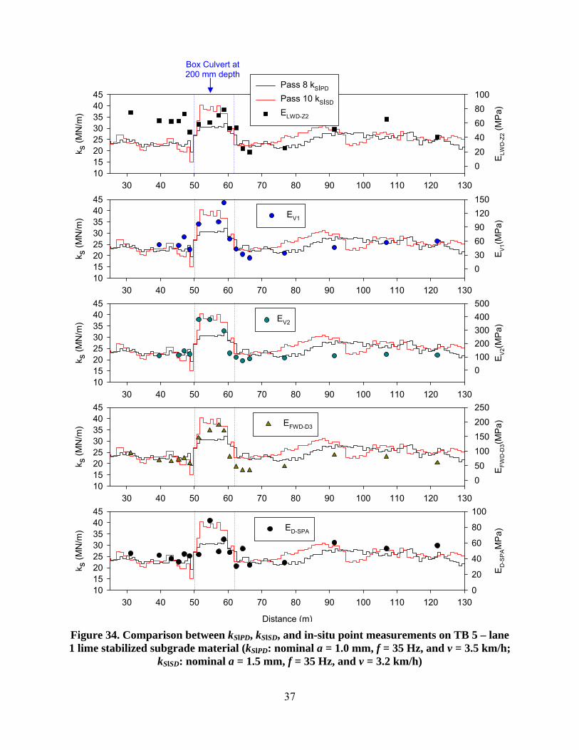
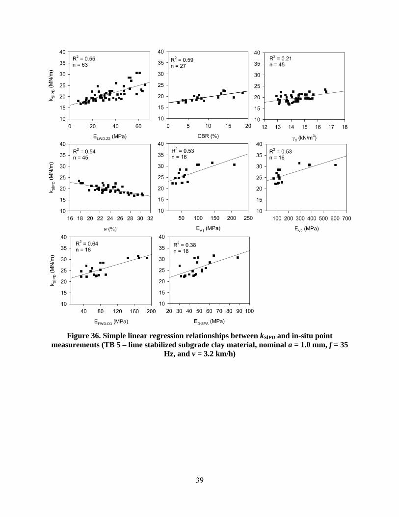
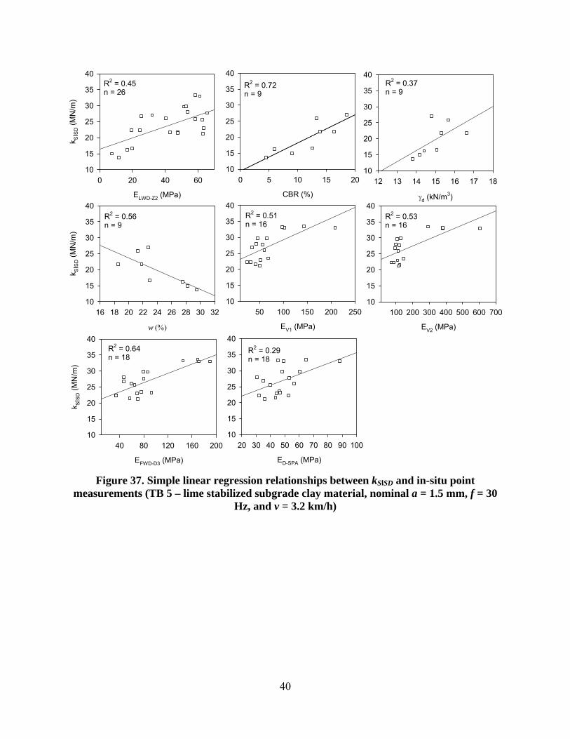
measurements indicating that an increase in w causes a decrease in ksΙPD. Using the mapping pass measurements from the smooth drum roller, ksΙSD measurements are also presented in comparison with the in-situ point measurements in Figure 33 and Figure 34. Discussion on comparison between ksΙSD and ksΙPD measurements is presented later in the report. Figure 35 shows the ksΙSD map with CBR profiles at four select locations highlighting the area underlain by box culvert. The ksΙSD values at the location underlain by the box culvert (about 200 mm below grade) were higher and the ksΙSD values were lower along the edge of the culvert, which is a common condition whereby it is difficult to compact material directly adjacent to box culvert walls. CBR profiles shown in Figure 35 confirm the poor backfill compaction condition. Simple linear regression relationships between ks values and different in-situ point measurements from are presented in Figure 36 and Figure 37. The relationships were developed by pairing spatially nearest point measurements with the ks data. Spatial locations of point measurements were slightly (< ± 0.5 m) adjusted to pair with appropriate roller measurement value using judgment. A summary of the regression relationships are presented in Table 5. The relationships show low R2 values for relationships with d (R

2 = 0.21 to 0.37). Relationships with ED-SPA for this dataset also show poor correlations, however with encouraging trends and warrants application in future studies. Other in-situ point measurements showed good correlations with R2 > 0.5. The ks values were sensitive to moisture content as evidenced by R2 > 0.5 in the regression relationships.

Summary

Both padfoot and smooth drum roller-integrated ks values (ksΙPD and ksΙSD) reliably

indicated the compaction quality of the lime stabilized subgrade clay material with good repeatability. The ks measurements effectively identified poor backfill compaction conditions along the edge of a box culvert located in this test bed and the results were confirmed from CBR profiles. Regression relationships between ks and different in-situ point measurements show positive correlations with varying degree of uncertainty in the correlations (as assessed by the R2 values), however. Better correlations were observed with EFWD, EV1, EV2, and ELWD values (with R2 > 0.5) compared to ED-SPA and d. Relationships with ED-SPA show encouraging trends in the data, however. The ks values were sensitive to moisture content of the compaction layer material.

Distance (m)

30 40 50 60 70 80 90 100 110 120 130

k s (M

N/m

)

10

15

20

25

30

35

40Pass 1Pass 4Pass 6Pass 8Pass 12

Box Culvert

35

Figure 30. kSΙPD measurements from different passes on TB5 lane 3 calibration test strip (nominal a = 1.0 mm, f = 35 Hz, and v = 3.5 km/h)

0 2 4 6 8 10 12 14

Ave

rag

e k S

IPD(M

N/m

)

18

19

20

21

22

23

24

25

0 2 4 6 8 10 12 14A

vera

ge

ELW

D-Z

2 (M

Pa)

20

25

30

35

40

45

50

Pass

0 2 4 6 8 10 12 14

Ave

rag

e

d (k

N/m

3 )

8

10

12

14

16

18

20

Pass

0 2 4 6 8 10 12 14

Ave

rag

e w

(%

)

18

20

22

24

26

28Pass

0 2 4 6 8 10 12 14

Ave

rag

e C

BR

(%

)

0

5

10

15

20

Figure 31. Compaction growth curves for kSΙPD and in-situ point measurements (TB 5 lane 3 calibration test strip, nominal a = 1.0 mm, f = 35 Hz, and v = 3.5 km/h)

0 2 4 6 8 10 12 14

Ave

rag

e k S

IPD (

MN

/m)

18

19

20

21

22

23

24

25

0 2 4 6 8 10 12 14

Ave

rag

e E

LWD

-Z2

(MP

a)

20

25

30

35

40

45

50

Pass

0 2 4 6 8 10 12 14

Ava

reag

e d

(kN

/m3 )

8

10

12

14

16

18

20

Pass

0 2 4 6 8 10 12 14

w (

%)

18

20

22

24

26

28Pass

0 2 4 6 8 10 12 14

Ave

rag

e C

BR

(%

)

0

5

10

15

20

NO DATA*

Figure 32. Compaction growth curves for in-situ point measurements (TB 5 lane 4 calibration test strip) (*roller data file corrupt)

36

40 60 80 100 12020 40 60 80 100 120

k s (M

N/m

)

10152025303540

40 60 80 100 120 40 60 80 100 120

Distance (m)

40 60 80 100 120

ELW

D-Z

2 (

MP

a)

0

30

60

90

120Pass 1 Pass 2 Pass 4 Pass 8

Pass 12kSIPD

40 60 80 100 12020 40 60 80 100 120

k s (M

N/m

)

10152025303540

40 60 80 100 120 40 60 80 100 120 40 60 80 100 120

CB

R (

%)

0

10

20

30Pass 1 Pass 2 Pass 4 Pass 8

40 60 80 100 12020 40 60 80 100 120

k s (M

N/m

)

10152025303540

40 60 80 100 120 40 60 80 100 120 40 60 80 100 120

w (

%)

0

10

20

30

Pass 1 Pass 2 Pass 4 Pass 8

40 60 80 100 12020 40 60 80 100 120

k s (M

N/m

)

10152025303540

40 60 80 100 120 40 60 80 100 120 40 60 80 100 120

d (

kN/m

3)

10121416182022

Pass 1 Pass 2 Pass 4 Pass 8

Pass 13 kSISD

Pass 12kSIPD

Pass 13 kSISD

Pass 12kSIPD

Pass 13 kSISD

Pass 12kSIPD

Pass 13 kSISD

Figure 33. Comparison results between kSΙPD (passes 1 to 12), kSΙSD (pass 13), and in-situ point measurements – TB5 lime stabilized subgrade calibration lane (nominal a = 1.0 mm, f = 35 Hz, and v = 3.5 km/h)

Box Culvert

37

30 40 50 60 70 80 90 100 110 120 130

k s (

MN

/m)

1015202530354045

EL

WD

-Z2 (

MP

a)

0

20

40

60

80

100Pass 8 kSIPD

Pass 10 kSISD

ELWD-Z2

30 40 50 60 70 80 90 100 110 120 130

k s (

MN

/m)

1015202530354045

EV

1(M

Pa)

0

30

60

90

120

150

EV1

30 40 50 60 70 80 90 100 110 120 130

k s (

MN

/m)

1015202530354045

EV

2(M

Pa)

0

100

200

300

400

500

EV2

30 40 50 60 70 80 90 100 110 120 130

k s (

MN

/m)

1015202530354045

EF

WD

-D3(M

Pa)

0

50

100

150

200

250

EFWD-D3

Distance (m)

30 40 50 60 70 80 90 100 110 120 130

k s (

MN

/m)

1015202530354045

ED

-SP

AM

Pa)

0

20

40

60

80

100

ED-SPA

Figure 34. Comparison between kSΙPD, kSΙSD, and in-situ point measurements on TB 5 – lane 1 lime stabilized subgrade material (kSΙPD: nominal a = 1.0 mm, f = 35 Hz, and v = 3.5 km/h;

kSΙSD: nominal a = 1.5 mm, f = 35 Hz, and v = 3.2 km/h)

Box Culvert at 200 mm depth

38

CBR (%)

0 10 20 30 40 50 60

Dep

th (

mm

)

0

200

400

600

800

Point 13

CBR (%)

0 10 20 30 40 50 60

Dep

th (

mm

)

0

200

400

600

800

Point 12

DCP refusal(Box Culvert)

CBR (%)

0 10 20 30 40 50 60

Dep

th (

mm

)

0

200

400

600

800

Point 5

CBR (%)

0 10 20 30 40 50 60

Dep

th (

mm

)

0

200

400

600

800

Point 1

Point 1

Point 5

Point 12

Point 13

w = 29.5% d = 13.8 kN/m3

ELWD‐Z2 = 11.6 MPa

ELWD‐Z2 = 58.4 MPaEV1 = 96.9 MPaEV2 = 381.1 MPaEFWD‐D3 = 145 MPaED‐SPA = 88 MPa

w = 20.8% d = 16.0 kN/m3

ELWD‐Z2 = 61.1 MPa

ELWD‐Z2 = 47.5 MPaEV1 = 42.1 MPaEV2 = 121.1 MPaEFWD‐D3 = 57 MPaED‐SPA = 44 MPa

Figure 35. kSΙSD maps (map 1: nominal a = 1.5 mm, f = 30 Hz, and v = 3.2 km/h) and DCP profiles at select locations on TB5 lime stabilized material (isolated area underlain by a

concrete box culvert)

This area comparatively wetter

39

w

16 18 20 22 24 26 28 30 32

k SIP

D (

MN

/m)

10

15

20

25

30

35

40

EV2 (MPa)

100 200 300 400 500 600 70010

15

20

25

30

35

40

ELWD-Z2 (MPa)

0 20 40 60

k SIP

D (

MN

/m)

10

15

20

25

30

35

40

CBR (%)

0 5 10 15 2010

15

20

25

30

35

40

d (kN/m3)

12 13 14 15 16 17 1810

15

20

25

30

35

40R2 = 0.55n = 63

EV1 (MPa)

50 100 150 200 25010

15

20

25

30

35

40

EFWD-D3 (MPa)

40 80 120 160 200

k SIP

D (

MN

/m)

10

15

20

25

30

35

40

ED-SPA (MPa)

20 30 40 50 60 70 80 90 10010

15

20

25

30

35

40

R2 = 0.59n = 27

R2 = 0.21n = 45

R2 = 0.54n = 45

R2 = 0.53n = 16

R2 = 0.53n = 16

R2 = 0.64n = 18

R2 = 0.38n = 18

Figure 36. Simple linear regression relationships between kSΙPD and in-situ point measurements (TB 5 – lime stabilized subgrade clay material, nominal a = 1.0 mm, f = 35

Hz, and v = 3.2 km/h)

40

w

16 18 20 22 24 26 28 30 32

k SIS

D (

MN

/m)

10

15

20

25

30

35

40

EV2 (MPa)

100 200 300 400 500 600 70010

15

20

25

30

35

40

ELWD-Z2 (MPa)

0 20 40 60

k SIS

D (

MN

/m)

10

15

20

25

30

35

40

CBR (%)

0 5 10 15 2010

15

20

25

30

35

40

d (kN/m3)

12 13 14 15 16 17 1810

15

20

25

30

35

40R2 = 0.45n = 26

EV1 (MPa)

50 100 150 200 25010

15

20

25

30

35

40

EFWD-D3 (MPa)

40 80 120 160 200

k SIS

D (

MN

/m)

10

15

20

25

30

35

40

ED-SPA (MPa)

20 30 40 50 60 70 80 90 10010

15

20

25

30

35

40

R2 = 0.72n = 9

R2 = 0.37n = 9

R2 = 0.56n = 9

R2 = 0.51n = 16

R2 = 0.53n = 16

R2 = 0.64n = 18

R2 = 0.29n = 18

Figure 37. Simple linear regression relationships between kSΙSD and in-situ point measurements (TB 5 – lime stabilized subgrade clay material, nominal a = 1.5 mm, f = 30

Hz, and v = 3.2 km/h)

41

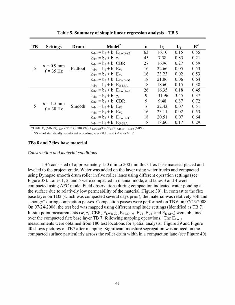
Table 5. Summary of simple linear regression analysis – TB 5

TB Settings Drum Model*

n b0 b1 R2

5 a = 0.9 mm f = 35 Hz

Padfoot

kSIPD = b0 + b1 ELWD-Z2 63 16.10 0.15 0.55 kSIPD = b0 + b1 d 45 7.58 0.85 0.21 kSIPD = b0 + b1 CBR 27 16.96 0.27 0.59 kSIPD = b0 + b1 EV1 16 22.66 0.05 0.53 kSIPD = b0 + b1 EV2 16 23.23 0.02 0.53 kSIPD = b0 + b1 EFWD-D3 18 21.06 0.06 0.64 kSIPD = b0 + b1 ED-SPA 18 18.60 0.15 0.38

5 a = 1.5 mm f = 30 Hz

Smooth

kSISD = b0 + b1 ELWD-Z2 26 16.35 0.18 0.45 kSISD = b0 + b1 d 9 -31.96 3.45 0.37 kSISD = b0 + b1 CBR 9 9.48 0.87 0.72 kSISD = b0 + b1 EV1 16 22.43 0.07 0.51 kSISD = b0 + b1 EV2 16 23.11 0.02 0.53 kSISD = b0 + b1 EFWD-D3 18 20.51 0.07 0.64 kSISD = b0 + b1 ED-SPA 18 18.60 0.17 0.29

*Units: ks (MN/m), d (kN/m3), CBR (%), ELWD-Z2/EV1/EV2/EFWD-D3/ED-SPA (MPa). † NS – not statistically significant according to p < 0.10 and t < -2 or > +2.

TBs 6 and 7 flex base material

Construction and material conditions

TB6 consisted of approximately 150 mm to 200 mm thick flex base material placed and

leveled to the project grade. Water was added on the layer using water trucks and compacted using Dynapac smooth drum roller in five roller lanes using different operation settings (see Figure 38). Lanes 1, 2, and 5 were compacted in manual mode, and lanes 3 and 4 were compacted using AFC mode. Field observations during compaction indicated water ponding at the surface due to relatively low permeability of the material (Figure 39). In contrast to the flex base layer on TB2 (which was compacted several days prior), the material was relatively soft and “spongy” during compaction passes. Compaction passes were performed on TB 6 on 07/23/2008. On 07/24/2008, the test bed was mapped using different amplitude settings (identified as TB 7). In-situ point measurements (w, d, CBR, ELWD-Z2, EFWD-D3, EV1, EV2, and ED-SPA) were obtained over the compacted flex base layer TB 7, following mapping operations. The EFWD measurements were obtained from 180 test locations for spatial analysis. Figure 39 and Figure 40 shows pictures of TB7 after mapping. Significant moisture segregation was noticed on the compacted surface particularly across the roller drum width in a compaction lane (see Figure 40).

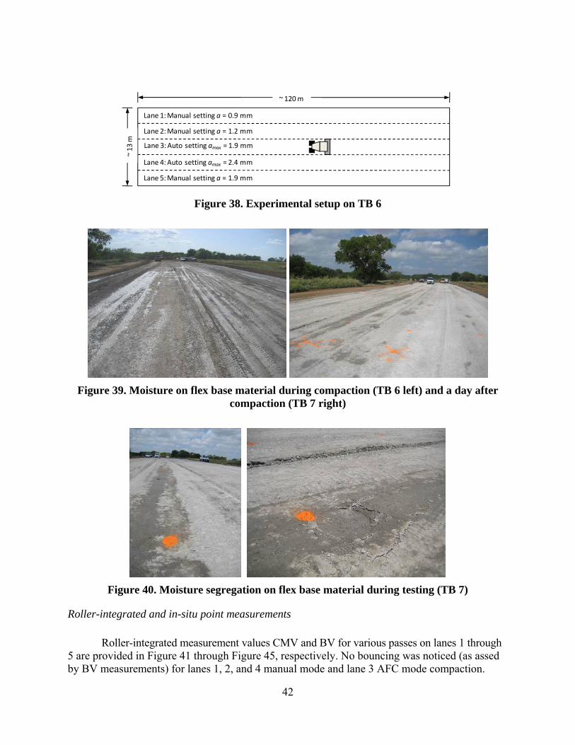
42

Lane 5: Manual setting a = 1.9 mm

Lane 4: Auto setting amax = 2.4 mm

Lane 2: Manual setting a = 1.2 mm

Lane 1: Manual setting a = 0.9 mm

~ 120 m

~ 13

 m

Lane 3: Auto setting amax = 1.9 mm

Figure 38. Experimental setup on TB 6

Figure 39. Moisture on flex base material during compaction (TB 6 left) and a day after compaction (TB 7 right)

Figure 40. Moisture segregation on flex base material during testing (TB 7)

Roller-integrated and in-situ point measurements

Roller-integrated measurement values CMV and BV for various passes on lanes 1 through

5 are provided in Figure 41 through Figure 45, respectively. No bouncing was noticed (as assed by BV measurements) for lanes 1, 2, and 4 manual mode and lane 3 AFC mode compaction.

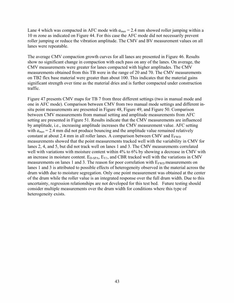
43

Lane 4 which was compacted in AFC mode with amax = 2.4 mm showed roller jumping within a 10 m zone as indicated on Figure 44. For this case the AFC mode did not necessarily prevent roller jumping or reduce the vibration amplitude. The CMV and BV measurement values on all lanes were repeatable.

The average CMV compaction growth curves for all lanes are presented in Figure 46. Results show no significant change in compaction with each pass on any of the lanes. On average, the CMV measurements were greater for lanes compacted with higher amplitudes. The CMV measurements obtained from this TB were in the range of 20 and 70. The CMV measurements on TB2 flex base material were greater than about 100. This indicates that the material gains significant strength over time as the material dries and is further compacted under construction traffic. Figure 47 presents CMV maps for TB 7 from three different settings (two in manual mode and one in AFC mode). Comparison between CMV from two manual mode settings and different in-situ point measurements are presented in Figure 48, Figure 49, and Figure 50. Comparison between CMV measurements from manual setting and amplitude measurements from AFC setting are presented in Figure 51. Results indicate that the CMV measurements are influenced by amplitude, i.e., increasing amplitude increases the CMV measurement value. AFC setting with amax = 2.4 mm did not produce bouncing and the amplitude value remained relatively constant at about 2.4 mm in all roller lanes. A comparison between CMV and EFWD

measurements showed that the point measurements tracked well with the variability in CMV for lanes 2, 4, and 5, but did not track well on lanes 1 and 3. The CMV measurements correlated well with variations with moisture content within 4% to 6% by showing a decrease in CMV with an increase in moisture content. ED-SPA, EV1, and CBR tracked well with the variations in CMV measurements on lanes 1 and 3. The reason for poor correlation with EFWD measurements on lanes 1 and 3 is attributed to possible effects of heterogeneity observed in the material across the drum width due to moisture segregation. Only one point measurement was obtained at the center of the drum while the roller value is an integrated response over the full drum width. Due to this uncertainty, regression relationships are not developed for this test bed. Future testing should consider multiple measurements over the drum width for conditions where this type of heterogeneity exists.

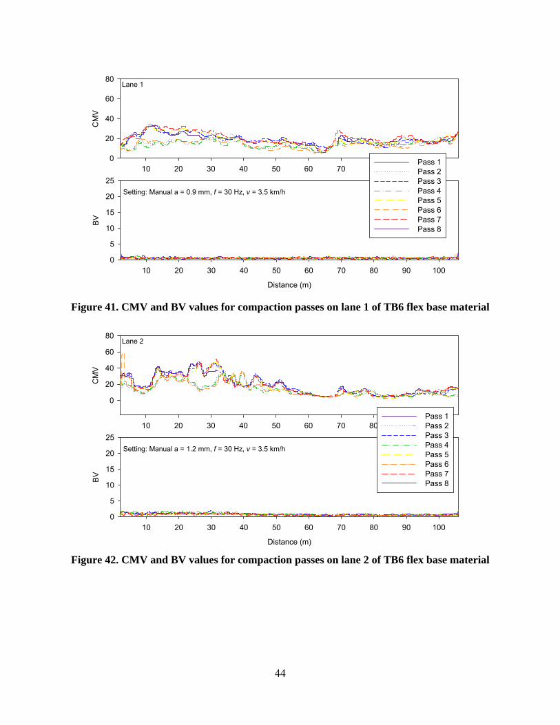
44

Distance (m)

10 20 30 40 50 60 70 80 90 100

BV

0

5

10

15

20

25

10 20 30 40 50 60 70 80 90 100

CM

V

0

20

40

60

80

Pass 1Pass 2Pass 3Pass 4Pass 5Pass 6Pass 7Pass 8

Setting: Manual a = 0.9 mm, f = 30 Hz, v = 3.5 km/h

Lane 1

Figure 41. CMV and BV values for compaction passes on lane 1 of TB6 flex base material

Distance (m)

10 20 30 40 50 60 70 80 90 100

BV

0

5

10

15

20

25

10 20 30 40 50 60 70 80 90 100

CM

V

0

20

40

60

80

Pass 1Pass 2Pass 3Pass 4Pass 5Pass 6Pass 7Pass 8

Setting: Manual a = 1.2 mm, f = 30 Hz, v = 3.5 km/h

Lane 2

Figure 42. CMV and BV values for compaction passes on lane 2 of TB6 flex base material

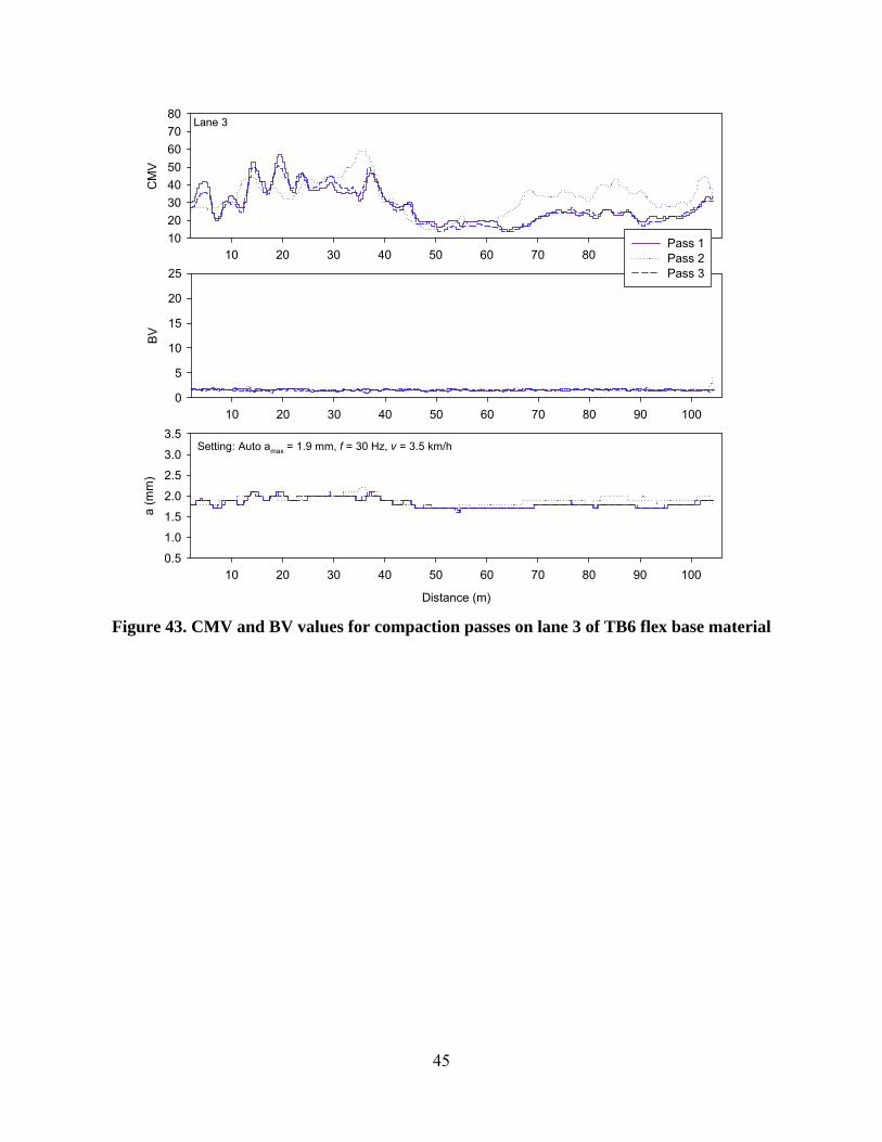
45

Distance (m)

10 20 30 40 50 60 70 80 90 100

a (

mm

)

0.5

1.0

1.5

2.0

2.5

3.0

3.5

10 20 30 40 50 60 70 80 90 100

BV

0

5

10

15

20

25

10 20 30 40 50 60 70 80 90 100

CM

V

10

20

30

40

50

60

70

80

Pass 1Pass 2Pass 3

Setting: Auto amax = 1.9 mm, f = 30 Hz, v = 3.5 km/h

Lane 3

Figure 43. CMV and BV values for compaction passes on lane 3 of TB6 flex base material

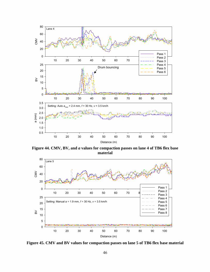
46

10 20 30 40 50 60 70 80 90 100

BV

0

5

10

15

20

25

10 20 30 40 50 60 70 80 90 100

CM

V

0

20

40

60

80

Pass 1Pass 2Pass 3Pass 4Pass 5Pass 6

Lane 4

Distance (m)

10 20 30 40 50 60 70 80 90 100

a (m

m)

0.5

1.0

1.5

2.0

2.5

3.0

3.5Setting: Auto amax = 2.4 mm, f = 30 Hz, v = 3.5 km/h

Figure 44. CMV, BV, and a values for compaction passes on lane 4 of TB6 flex base material

Distance (m)

10 20 30 40 50 60 70 80 90 100

BV

0

5

10

15

20

25

10 20 30 40 50 60 70 80 90 100

CM

V

0

20

40

60

80

Pass 1Pass 2Pass 3Pass 4Pass 5Pass 6Pass 7Pass 8

Setting: Manual a = 1.9 mm, f = 30 Hz, v = 3.5 km/h

Lane 5

Figure 45. CMV and BV values for compaction passes on lane 5 of TB6 flex base material

Drum bouncing

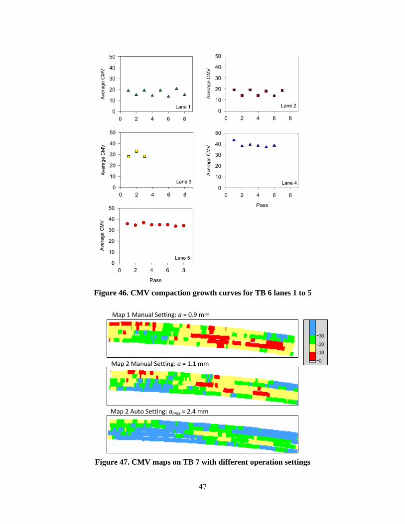
47

0 2 4 6 8

Ave

rag

e C

MV

0

10

20

30

40

50

0 2 4 6 8

Ave

rag

e C

MV

0

10

20

30

40

50

0 2 4 6 8

Ave

rag

e C

MV

0

10

20

30

40

50

Pass

0 2 4 6 8

Ave

rag

e C

MV

0

10

20

30

40

50

Pass

0 2 4 6 8

Ave

rag

e C

MV

0

10

20

30

40

50

Lane 1 Lane 2

Lane 3 Lane 4

Lane 5

Figure 46. CMV compaction growth curves for TB 6 lanes 1 to 5

Figure 47. CMV maps on TB 7 with different operation settings

Map 1 Manual Setting: a = 0.9 mm 

Map 2 Manual Setting: a = 1.1 mm 

Map 2 Auto Setting: amax = 2.4 mm 

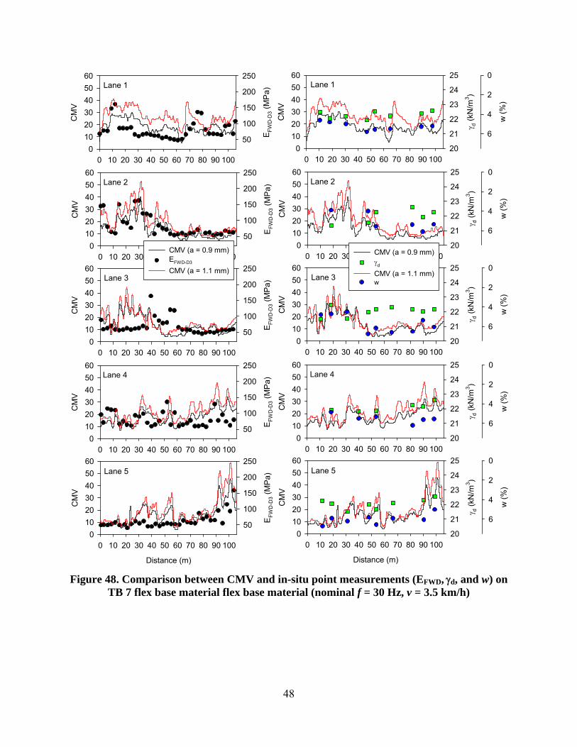
48

0 10 20 30 40 50 60 70 80 90 100

CM

V

0

10

20

30

40

50

60

EF

WD

-D3 (

MP

a)

50

100

150

200

250

0 10 20 30 40 50 60 70 80 90 100

CM

V

0

10

20

30

40

50

60

EF

WD

-D3

(MP

a)

50

100

150

200

250

0 10 20 30 40 50 60 70 80 90 100

CM

V

0

10

20

30

40

50

60

EF

WD

-D3

(MP

a)

50

100

150

200

250

0 10 20 30 40 50 60 70 80 90 100

CM

V

0

10

20

30

40

50

60E

FW

D-D

3 (M

Pa)

50

100

150

200

250

CMV (a = 0.9 mm)EFWD-D3

CMV (a = 1.1 mm)

Distance (m)

0 10 20 30 40 50 60 70 80 90 100

CM

V

0

10

20

30

40

50

60

EF

WD

-D3

(MP

a)

50

100

150

200

250

Lane 1

Lane 2

Lane 3

Lane 4

Lane 5

0 10 20 30 40 50 60 70 80 90 100

CM

V

0

10

20

30

40

50

60

d (

kN/m

3)

20

21

22

23

24

25

w (

%)

0

2

4

6

0 10 20 30 40 50 60 70 80 90 100

CM

V

0

10

20

30

40

50

60

d (

kN/m

3 )

20

21

22

23

24

25

w (

%)

0

2

4

6

0 10 20 30 40 50 60 70 80 90 100

CM

V

0

10

20

30

40

50

60

d (

kN/m

3 )

20

21

22

23

24

25

w (

%)

0

2

4

6

0 10 20 30 40 50 60 70 80 90 100

CM

V

0

10

20

30

40

50

60

d (

kN/m

3 )

20

21

22

23

24

25

w (

%)

0

2

4

6

CMV (a = 0.9 mm)d

CMV (a = 1.1 mm)w

Distance (m)

0 10 20 30 40 50 60 70 80 90 100

CM

V

0

10

20

30

40

50

60 d

(kN

/m3 )

20

21

22

23

24

25

w (

%)

0

2

4

6

Lane 1

Lane 2

Lane 3

Lane 4

Lane 5

Figure 48. Comparison between CMV and in-situ point measurements (EFWD, d, and w) on TB 7 flex base material flex base material (nominal f = 30 Hz, v = 3.5 km/h)

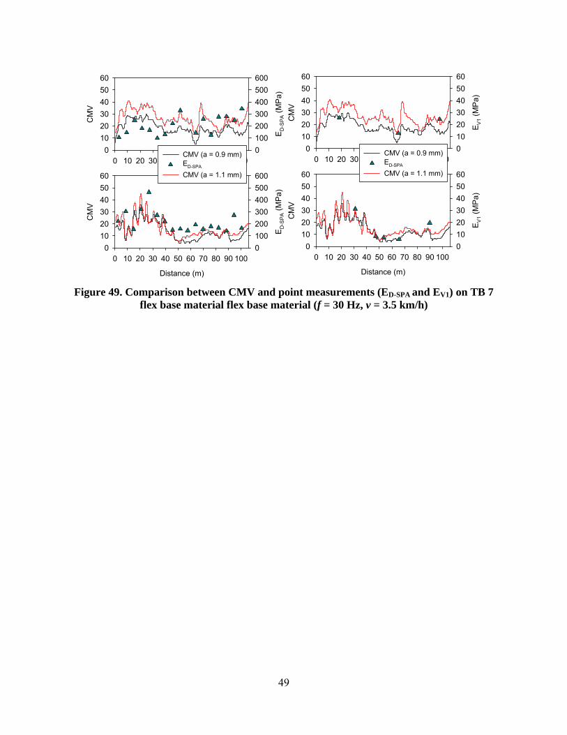
49

0 10 20 30 40 50 60 70 80 90 100

CM

V

0

10

20

30

40

50

60

ED

-SP

A (

MP

a)

0

100

200

300

400

500

600

Distance (m)

0 10 20 30 40 50 60 70 80 90 100

CM

V

0

10

20

30

40

50

60

ED

-SP

A (

MP

a)

0

100

200

300

400

500

600

CMV (a = 0.9 mm)ED-SPA

CMV (a = 1.1 mm)

0 10 20 30 40 50 60 70 80 90 100

CM

V

0

10

20

30

40

50

60

EV

1 (M

Pa

)

0

10

20

30

40

50

60

Distance (m)

0 10 20 30 40 50 60 70 80 90 100

CM

V

0

10

20

30

40

50

60

EV

1 (

MP

a)

0

10

20

30

40

50

60

CMV (a = 0.9 mm)ED-SPA

CMV (a = 1.1 mm)

Figure 49. Comparison between CMV and point measurements (ED-SPA and EV1) on TB 7 flex base material flex base material (f = 30 Hz, v = 3.5 km/h)

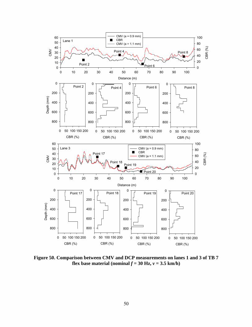
50

Distance (m)

0 10 20 30 40 50 60 70 80 90 100

CM

V

0

10

20

30

40

50

60

CB

R (

%)

0

20

40

60

80

100Lane 1

CBR (%)

0 50 100 150 200

De

pth

(m

m)

0

200

400

600

800

CBR (%)

0 50 100 150 200

0

200

400

600

800

CBR (%)

0 50 100 150 200

0

200

400

600

800

CBR (%)

0 50 100 150 200

0

200

400

600

800

Point 2 Point 4 Point 6 Point 8

Distance (m)

0 10 20 30 40 50 60 70 80 90 100

CM

V

0

10

20

30

40

50

60

CB

R (

%)

0

20

40

60

80

100

CMV (a = 0.9 mm)CBRCMV (a = 1.1 mm)

Lane 3

Point 2

Point 4

Point 6

Point 8

CBR (%)

0 50 100 150 200

Dep

th (

mm

)

0

200

400

600

800

CBR (%)

0 50 100 150 200

0

200

400

600

800

CBR (%)

0 50 100 150 200

0

200

400

600

800

CBR (%)

0 50 100 150 200

0

200

400

600

800

CMV (a = 0.9 mm)CBRCMV (a = 1.1 mm)

Point 17

Point 18Point 19

Point 20

Point 17 Point 18 Point 19 Point 20

Figure 50. Comparison between CMV and DCP measurements on lanes 1 and 3 of TB 7 flex base material (nominal f = 30 Hz, v = 3.5 km/h)

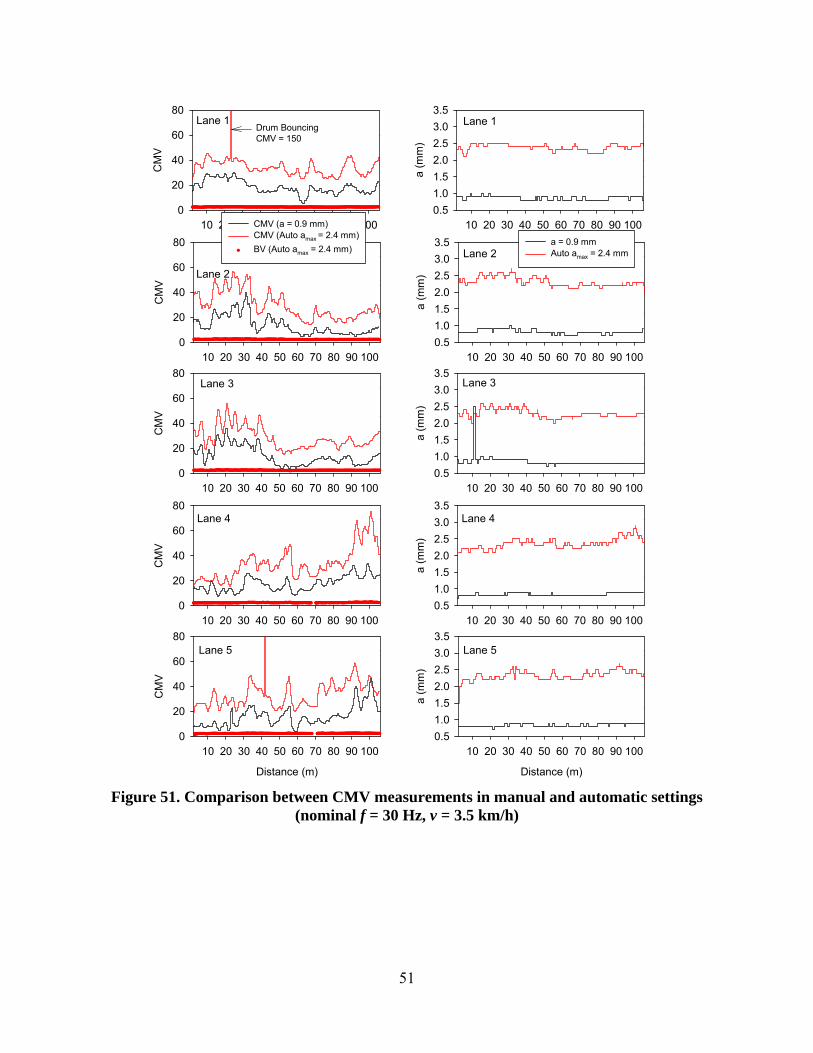
51

10 20 30 40 50 60 70 80 90 100

a (m

m)

0.5

1.0

1.5

2.0

2.5

3.0

3.5

10 20 30 40 50 60 70 80 90 100

CM

V

0

20

40

60

80

10 20 30 40 50 60 70 80 90 100

CM

V

0

20

40

60

80

CMV (a = 0.9 mm)CMV (Auto amax = 2.4 mm)

BV (Auto amax = 2.4 mm)

10 20 30 40 50 60 70 80 90 100

CM

V

0

20

40

60

80

10 20 30 40 50 60 70 80 90 100

CM

V

0

20

40

60

80

Distance (m)

10 20 30 40 50 60 70 80 90 100

CM

V

0

20

40

60

80

Lane 1

Lane 2

Lane 3

Lane 4

Lane 5

10 20 30 40 50 60 70 80 90 100

a (m

m)

0.5

1.0

1.5

2.0

2.5

3.0

3.5

10 20 30 40 50 60 70 80 90 100

a (m

m)

0.5

1.0

1.5

2.0

2.5

3.0

3.5

10 20 30 40 50 60 70 80 90 100

a (m

m)

0.5

1.0

1.5

2.0

2.5

3.0

3.5 a = 0.9 mmAuto amax = 2.4 mm

Distance (m)

10 20 30 40 50 60 70 80 90 100

a (

mm

)

0.5

1.0

1.5

2.0

2.5

3.0

3.5

Lane 1

Lane 2

Lane 3

Lane 4

Lane 5

Drum BouncingCMV = 150

Figure 51. Comparison between CMV measurements in manual and automatic settings (nominal f = 30 Hz, v = 3.5 km/h)

52

Spatial analysis of roller-integrated and in-situ compaction measurements

Roller-integrated compaction measurements provide an opportunity to spatially visualize

and quantify “non-uniformity” of compaction measurement values. This topic is slowly gaining popularity among the pavement engineering community. Vennapusa and White (2008) demonstrated the use of semivariogram analysis in combination with conventional statistical analysis to effectively address the issue of non-uniformity in quality assurance during earthwork construction. A variogram is a plot of the average squared differences between data values as a function of separation distance, and is a common tool used in geostatistical studies to describe spatial variation. Three important features of a semivariogram include: sill, range, and nugget. Sill is defined as the plateau that the semivariogram reaches, range is defined as the distance at which the semivariogram reaches the sill, and nugget is defined as the vertical height of the discontinuity at the origin which mostly represents sampling error or short scale variations (Srivastava, 1996). From a semivariogram model, a low “sill” and longer “range of influence” can represent best conditions for uniformity, while the opposite represents an increasingly non-uniform condition. Using these semivariogram parameters, theoretical models can be fit to the experimental semivariogram data. In the author’s experience, exponential model generally fits well with the roller-integrated and in-situ compaction measurements (see White et al. 2007a, White et al. 2007b, Vennapusa and White 2008). Detailed descriptions of theoretical models can be found elsewhere in the literature (e.g., Clark and Harper 2002). To evaluate the application of spatial analysis, spatially referenced CMV and EFWD measurements obtained from TB 7 were analyzed. The comparisons are shown using theoretical and experimental semivariogram models, and Kriged surface maps generated for CMV and EFWD measurements using the theoretical (exponential) semivariogram model. The theoretical semivariograms were fit to the experimental semivariograms by checking for its “goodness” using the modified Cressie goodness of fit approach suggested by Clark and Harper (2002) as well as the cross-validation process. A lower Cressie “goodness” factor and high R2 value in cross-validation process indicates a better fit (see White et al. 2007a for additional details on model fitting process). The semivariograms of CMV for two different amplitude settings showed similar effective ranges (6 m) but with higher sill for a = 1.1 mm than for a = 0.9 mm. This means that CMV data obtained with a = 1.1 mm setting was relatively more non-uniform than obtained with a = 0.9 mm. Univariate statistics (mean , standard deviation , and coefficient of variation COV) presented on Figure 52 show that the CMV from a = 1.1 mm setting was slightly higher on average than the CMV from a = 0.9 mm but with similar COV, however. This demonstrates the advantage of using spatial statistics for a better characterization of non-uniform conditions than using univariate statistics. The reasons for a difference in sill values of CMV for different amplitude settings are attributed to the materials’ response to different stress conditions and possibly different influence depths. Increasing amplitude increases the contact stresses under the roller drum and also believed to increase the depth of influence under the drum. The EFWD

measurements showed slightly lower spatial continuity compared to CMV measurements with an effective range of about 4.5 m. The CMV and EFWD Kriged contour maps are spatially comparable and showed similar spatial structure in their respective semivariograms.

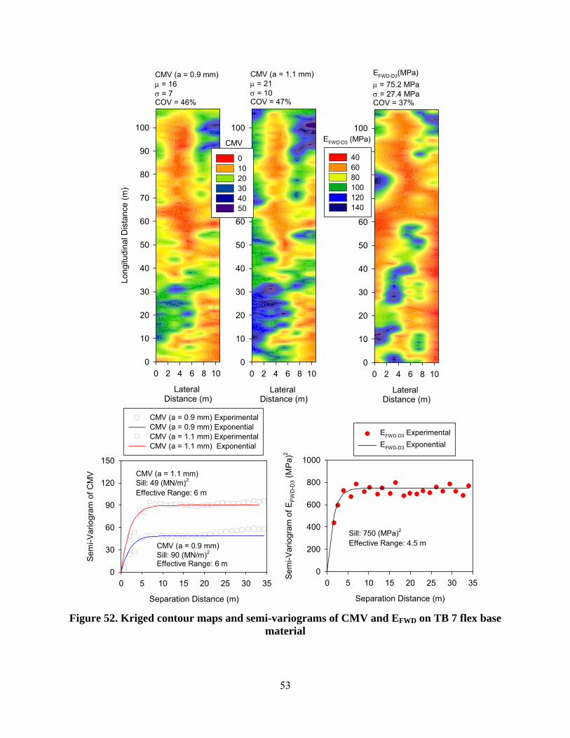
53

Lateral Distance (m)

0 2 4 6 8 100

10

20

30

40

50

60

70

80

90

100

Lateral Distance (m)

0 2 4 6 8 10

Lon

gitu

din

al D

ista

nce

(m)

0

10

20

30

40

50

60

70

80

90

100

0 10 20 30 40 50

Lateral Distance (m)

0 2 4 6 8 100

10

20

30

40

50

60

70

80

90

100

40 60 80 100 120 140

CMV (a = 0.9 mm) = 16 = 7COV = 46%

CMV (a = 1.1 mm) = 21 = 10COV = 47%

EFWD-D3(MPa)

= 75.2 MPa = 27.4 MPaCOV = 37%

CMV EFWD-D3 (MPa)

Separation Distance (m)

0 5 10 15 20 25 30 35

Sem

i-Var

iogr

am o

f C

MV

0

30

60

90

120

150

CMV (a = 0.9 mm) ExperimentalCMV (a = 0.9 mm) ExponentialCMV (a = 1.1 mm) ExperimentalCMV (a = 1.1 mm) Exponential

Separation Distance (m)

0 5 10 15 20 25 30 35

Sem

i-Var

iogr

am o

f E

FW

D-D

3 (M

Pa)

2

0

200

400

600

800

1000

EFWD-D3 Experimental

EFWD-D3 Exponential

CMV (a = 0.9 mm)Sill: 90 (MN/m)2

Effective Range: 6 m

CMV (a = 1.1 mm)Sill: 49 (MN/m)2

Effective Range: 6 m

Sill: 750 (MPa)2

Effective Range: 4.5 m

Figure 52. Kriged contour maps and semi-variograms of CMV and EFWD on TB 7 flex base material

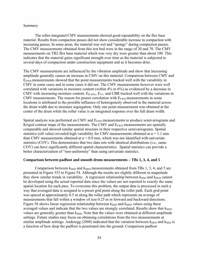
54

Summary

The roller-integrated CMV measurements showed good repeatability on the flex base

material. Results from compaction passes did not show considerable increase in compaction with increasing passes. In some areas, the material was wet and “spongy” during compaction passes. The CMV measurements obtained from this test bed were in the range of 20 and 70. The CMV measurements on TB2 flex base material which was very dry were greater than about 100. This indicates that the material gains significant strength over time as the material is subjected to several days of compaction under construction equipment and as it becomes drier.

The CMV measurements are influenced by the vibration amplitude and show that increasing amplitude generally causes an increase in CMV on this material. Comparison between CMV and EFWD measurements showed that the point measurements tracked well with the variability in CMV in some cases and in some cases it did not. The CMV measurements however were well correlated with variations in moisture content (within 4% to 6%) as evidenced by a decrease in CMV with increasing moisture content. ED-SPA, EV1, and CBR tracked well with the variations in CMV measurements. The reason for poorer correlation with EFWD measurements in some locations is attributed to the possible influence of heterogeneity observed in the material across the drum width due to moisture segregation. Only one point measurement was obtained at the center of the drum while the roller value is an integrated response over the full drum width. Spatial analysis was performed on CMV and EFWD measurements to produce semivariograms and Kriged contour maps of the measurements. The CMV and EFWD measurements are spatially comparable and showed similar spatial structure in their respective semivariograms. Spatial statistics (sill value) revealed high variability for CMV measurements obtained at a = 1.1 mm than CMV measurements obtained at a = 0.9 mm, which was not identified with univariate statistics (COV). This demonstrates that two data sets with identical distributions (i.e., same COV) can have significantly different spatial characteristics. Spatial statistics can provide a better characterization of “non-uniformity” than using univariate statistics.

Comparison between padfoot and smooth drum measurements – TBs 1, 3, 4, and 5

Comparison between kSΙSD and kSΙPD measurements obtained from TBs 1, 3, 4, and 5 are presented in Figure 553 to Figure 54. Although the results are slightly different in magnitude they show similar trends in variability. A regression relationship between kSΙSD and kSΙPD cannot be developed using the actual reported data since the values are not reported to exactly the same spatial location for each pass. To overcome this problem, the output data is processed in such a way that averaged data is assigned to a preset grid point along the roller path. Each grid point was spaced at approximately 0.5 m along the roller path which represents an average of measurements that fall within a window of size 0.25 m in forward and backward directions. Figure 56 shows linear regression relationship between kSΙSD and kSΙPD values using these averaged values and indicate that the two values are strongly correlated. Results show that kSΙPD values are generally greater than kSΙSD. Note that the values were obtained at different amplitude settings. Future studies may focus on obtaining correlations from the two measurements at similar amplitude settings. Anderegg (2008) indicated that the variation between kSΙPD and kSΙSD is a function of how deep the padfoot is penetrated into the ground. Comparison padfoot

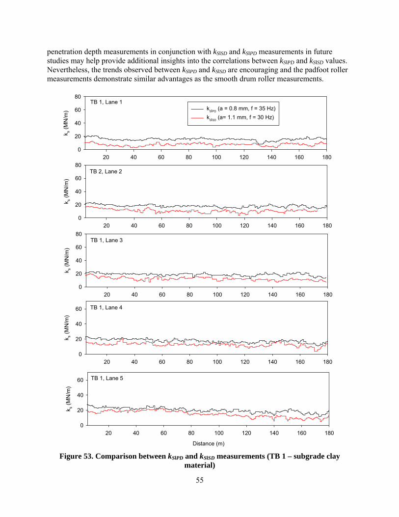
55

penetration depth measurements in conjunction with kSΙSD and kSΙPD measurements in future studies may help provide additional insights into the correlations between kSΙPD and kSΙSD values. Nevertheless, the trends observed between kSΙPD and kSΙSD are encouraging and the padfoot roller measurements demonstrate similar advantages as the smooth drum roller measurements.

20 40 60 80 100 120 140 160 180

k s (M

N/m

)

0

20

40

60

80

kSIPD

(a = 0.8 mm, f = 35 Hz)

kSISD

(a= 1.1 mm, f = 30 Hz)

20 40 60 80 100 120 140 160 180

k s (M

N/m

)

0

20

40

60

80

20 40 60 80 100 120 140 160 180

k s (M

N/m

)

0

20

40

60

80

20 40 60 80 100 120 140 160 180

k s (M

N/m

)

0

20

40

60

Distance (m)

20 40 60 80 100 120 140 160 180

k s (M

N/m

)

0

20

40

60

TB 1, Lane 1

TB 2, Lane 2

TB 1, Lane 3

TB 1, Lane 4

TB 1, Lane 5

Figure 53. Comparison between kSΙPD and kSΙSD measurements (TB 1 – subgrade clay material)

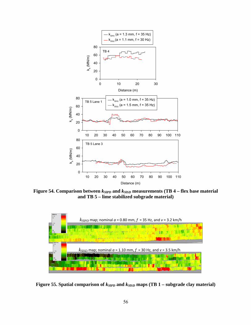
56

10 20 30 40 50 60 70 80 90 100 110

k s (M

N/m

)

0

20

40

60

80 kSIPD

(a = 1.0 mm, f = 35 Hz)

kSISD

(a = 1.5 mm, f = 35 Hz)

Distance (m)

10 20 30 40 50 60 70 80 90 100 110

k s (M

N/m

)

0

20

40

60

80

TB 5 Lane 1

TB 5 Lane 3

Distance (m)

0 10 20 30k s

(MN

/m)

0

20

40

60

80

kSIPD

(a = 1.3 mm, f = 35 Hz)

kSISD

(a = 1.1 mm, f = 30 Hz)

TB 4

Figure 54. Comparison between kSΙPD and kSΙSD measurements (TB 4 – flex base material and TB 5 – lime stabilized subgrade material)

Figure 55. Spatial comparison of kSΙPD and kSΙSD maps (TB 1 – subgrade clay material)

kSΙSD map; nominal a = 1.10 mm, f  = 30 Hz, and v = 3.5 km/h 

kSΙPD map; nominal a = 0.80 mm, f  = 35 Hz, and v = 3.2 km/h 

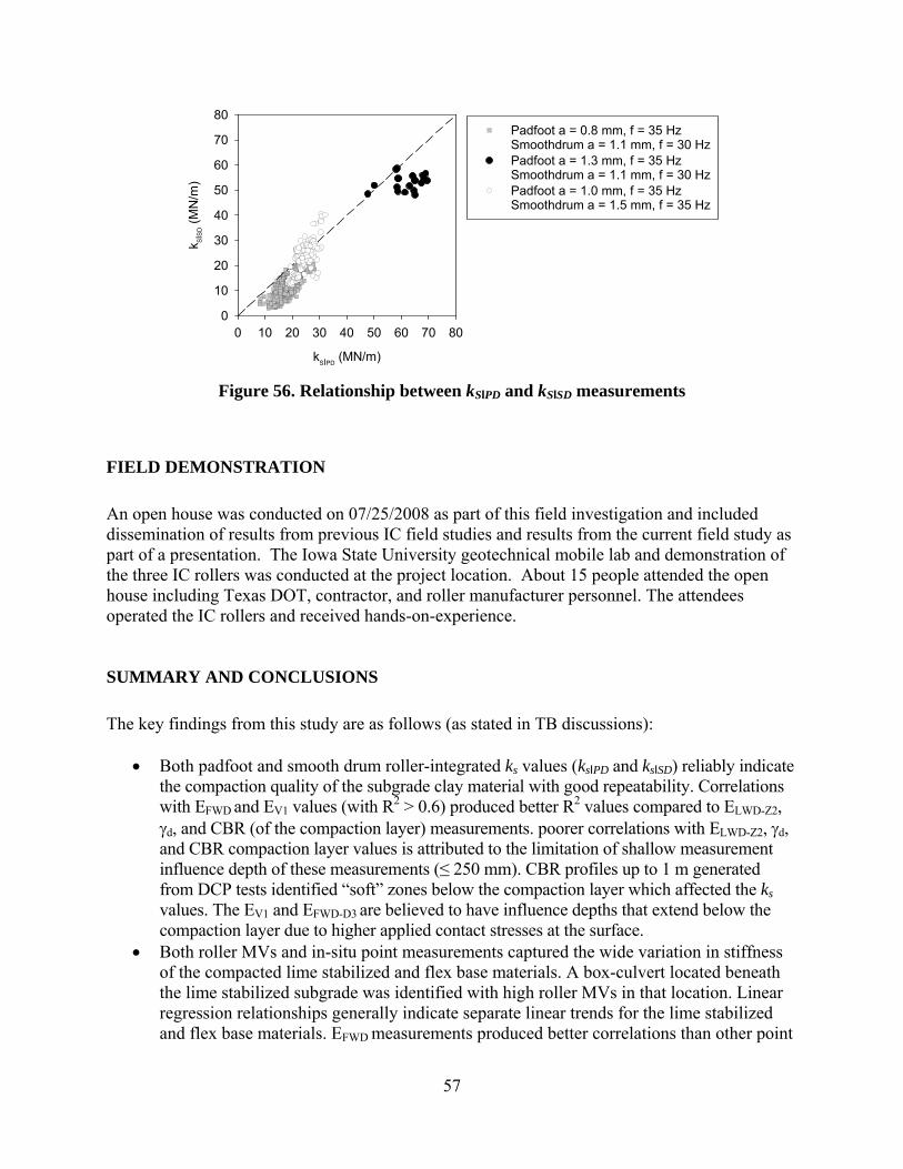
57

kSIPD

(MN/m)

0 10 20 30 40 50 60 70 80

k SIS

D (

MN

/m)

0

10

20

30

40

50

60

70

80Padfoot a = 0.8 mm, f = 35 HzSmoothdrum a = 1.1 mm, f = 30 HzPadfoot a = 1.3 mm, f = 35 HzSmoothdrum a = 1.1 mm, f = 30 HzPadfoot a = 1.0 mm, f = 35 HzSmoothdrum a = 1.5 mm, f = 35 Hz

Figure 56. Relationship between kSΙPD and kSΙSD measurements

FIELD DEMONSTRATION

An open house was conducted on 07/25/2008 as part of this field investigation and included dissemination of results from previous IC field studies and results from the current field study as part of a presentation. The Iowa State University geotechnical mobile lab and demonstration of the three IC rollers was conducted at the project location. About 15 people attended the open house including Texas DOT, contractor, and roller manufacturer personnel. The attendees operated the IC rollers and received hands-on-experience. SUMMARY AND CONCLUSIONS

The key findings from this study are as follows (as stated in TB discussions):

Both padfoot and smooth drum roller-integrated ks values (ksΙPD and ksΙSD) reliably indicate the compaction quality of the subgrade clay material with good repeatability. Correlations with EFWD and EV1 values (with R2 > 0.6) produced better R2 values compared to ELWD-Z2, d, and CBR (of the compaction layer) measurements. poorer correlations with ELWD-Z2, d, and CBR compaction layer values is attributed to the limitation of shallow measurement influence depth of these measurements (≤ 250 mm). CBR profiles up to 1 m generated from DCP tests identified “soft” zones below the compaction layer which affected the ks values. The EV1 and EFWD-D3 are believed to have influence depths that extend below the compaction layer due to higher applied contact stresses at the surface.

Both roller MVs and in-situ point measurements captured the wide variation in stiffness of the compacted lime stabilized and flex base materials. A box-culvert located beneath the lime stabilized subgrade was identified with high roller MVs in that location. Linear regression relationships generally indicate separate linear trends for the lime stabilized and flex base materials. EFWD measurements produced better correlations than other point

58

measurements. Hyperbolic regression relationships were developed for EFWD and ED-SPA measurements which showed strong correlations with ks and CMV measurements but additional data is needed to validate the relationships. The CMV measurements at this location were highly repeatable.

Both padfoot and smooth drum roller-integrated ks values (ksΙPD and ksΙSD) reliably indicated the compaction quality of the lime stabilized subgrade clay material with good repeatability. The ks measurements effectively identified poor backfill compaction conditions along the edge of a box culvert located in this test bed and the results were confirmed from CBR profiles. Regression relationships between ks and different in-situ point measurements show positive correlations with varying degree of uncertainty in the correlations (as assessed by the R2 values), however. Better correlations were observed with EFWD, EV1, EV2, and ELWD values (with R2 > 0.5) compared to ED-SPA and d. Relationships with ED-SPA show encouraging trends in the data, however. The ks values were sensitive to moisture content of the compaction layer material.

The roller-integrated CMV measurements showed good repeatability on the flex base material. Results from compaction passes did not show considerable increase in compaction with increasing passes. In some areas, the material was wet and “spongy” during compaction passes. The CMV measurements obtained from this test bed were in the range of 20 and 70. The CMV measurements on TB2 flex base material which was very dry were greater than about 100. This indicates that the material gains significant strength over time as the material is subjected to several days of compaction under construction equipment and as it becomes drier.

The CMV measurements are influenced by the vibration amplitude and show that increasing amplitude generally causes an increase in CMV on this material. Comparison between CMV and EFWD measurements showed that the point measurements tracked well with the variability in CMV in some cases and in some cases it did not. The CMV measurements however were well correlated with variations in moisture content (within 4% to 6%) as evidenced by a decrease in CMV with increasing moisture content. ED-SPA, EV1, and CBR tracked well with the variations in CMV measurements. The reason for poorer correlation with EFWD measurements in some locations is attributed to the possible influence of heterogeneity observed in the material across the drum width due to moisture segregation. Only one point measurement was obtained at the center of the drum while the roller value is an integrated response over the full drum width.

Spatial analysis was performed on CMV and EFWD measurements to produce semivariograms and Kriged contour maps of the measurements. The CMV and EFWD measurements are spatially comparable and showed similar spatial structure in their respective semivariograms. Spatial statistics (sill value) revealed high variability for CMV measurements obtained at a = 1.1 mm than CMV measurements obtained at a = 0.9 mm, which was not identified with univariate statistics (COV). This demonstrates that two data sets with identical distributions (i.e., same COV) can have significantly different spatial characteristics. Spatial statistics can provide a better characterization of “non-uniformity” than using univariate statistics.

Comparison between kSΙSD and kSΙPD show that kSΙPD values are generally greater than kSΙSD. Note that the values were obtained at different amplitude settings. Future studies may focus on obtaining correlations from the two measurements at similar amplitude settings. Comparison padfoot penetration depth measurements in conjunction with kSΙSD

59

and kSΙPD measurements in future studies may help provide additional insights into the correlations between kSΙPD and kSΙSD values. Nevertheless, the trends observed between kSΙPD and kSΙSD are encouraging and the padfoot roller measurements demonstrate similar advantages as the smooth drum roller measurements.

60

REFERENCES

Anderegg, R. (1998). Nichtlineare Schwingungen bei dynamischen Bodenverdichtern. Ph.D. Dissertation, Eidgenossische Technische Hochschule Zurich (in German).

Anderegg, R., and Kaufmann, K. (2004). "Intelligent compaction with vibratory rollers." Transp.

Res. Rec., 1868, Journal of the Transportation Research Board, Washington D.C., 124–134. Anderegg, R. (2008). Testing the PD-Shell Single Drum Roller SV 212ACE. July 31

(unpublished report). Clark, I., and Harper, W. (2002). Practical geostatistics 2000. 3rd reprint, Ecosse North America

Llc, Columbus, Oh. Nazarian, S., Baker, M.R., and Crain, K. (1993). Fabrication and Testing of a Seismic Pavement

Analyzer. SHRP Report H-375. National Highway Research Council, Washington, D.C. Srivastava, R. M. (1996). “Describing spatial variability using geostatistical analysis.”

Geostatistics for Environmental and Geotechnical Applications, ASTM STP 1283, R. M. Srivastava, S. Rouhani, M. V. Cromer, A. J. Desbarats, A. I. Johnson, eds., ASTM, West Conshohocken, Pa, 13–19.

Vennapusa, P., White, D.J. (2008b). “Geostatistical analysis for spatially referenced roller-

integrated compaction measurements, Journal of Geotechnical and Geoenvironmental Engineering, ASCE (in review, submitted July 2008).

White, D.J, Thompson, M., Vennapusa, P. (2007a). Field Validation of Intelligent Compaction

Monitoring Technology for Unbound Materials, Mn/DOT Report No. MN/RC 2007-10, Iowa State University, Ames, IA.

White, D. J., Thompson, M., Vennapusa, P. (2007b). Field study of compaction monitoring

systems – Tamping foot 825 and vibratory smooth drum CS-533E rollers. Final Report, Center of Transportation Research and Education, Iowa State University, Ames, Ia.

White, D. J. (2008). Report of the Workshop on Intelligent Compaction for Soils and HMA.

Earthworks Engineering Research Center – Iowa State University and Iowa Department of Transportation, Ames, Iowa, April 2-4.

Yoo, T., Selig. E. (1980). “New concepts of vibratory compaction of soil,” Proc. of Intl. Conf. on

Compaction, Vol. II, Paris, pp. 703–707. Zorn, G. (2003). Operating manual: Light drop-weight tester ZFG2000, Zorn Stendal, Germany.

61

APPENDIX

62

Test Beds # 1/3 (07/21/2008 to 07/22/2008) Construction/Testing Photos

Description: The test bed was constructed by scarifying the existing subgrade material to a depth of about 250 mm (10 inches) and compacted in f ive lanes where two lanes (Lanes 4 and 5) were used as calibration test strips and the rest was used for production compaction. Lane 5 was prepared with three target moisture sections with moisture contents varying f rom dry to wet of the materials’ optimum moisture content. The Case/Ammann pad foot roller was used for compaction for passes 1 to 10 and smooth drum roller was used for mapping (passes 11 to 14). In-situ point measurements (w, d, CBR, and ELWD) were obtained af ter 1, 2, 4, and 8 roller passes. Some point locations along lanes 1 and 5 were selected for EFWD, EV1, and EV2 testing (denoted as TB3). The objectives of this test bed were to obtain correlations between padfoot roller MVs and in-situ soil properties, and compare padfoot and smooth drum roller MVs.

Machine settings: Passes 1 to 8 – f = 35 Hz, Ecc. = 33%, a ~ 0.8 mm; Pass 9 – f = 35 Hz, Ecc. = 41%, a ~ 0.95 mm; Pass 10 – f = 30 Hz, Ecc. = 67%, a ~ 1.3 mm; Mapping Pass 11 – f = 30 Hz, Ecc. = 66%, a ~ 2.0 mm; Pass 12 – f = 30 Hz, Ecc. = 33%, a ~ 1.1 mm; Passes 13 to 14 – f = 30 Hz, Ecc. = 90%, a ~ 2.0+ mm.

Subgrade scarification using grader

Compaction using Case/Ammann padfoot roller

Zorn LWD DCP

Calibration Test Strips

CalibrationPoint Measurements

Accelerated Implementation of IC Technology for Embankment Subgrade Soils, Aggregate Base, and Asphalt Pavement Materials

Iowa State University Research Team Field Testing, FM 156 Fort Worth, Texas

Lanes 1   2   3  4   5

~ 180m

~14 m

Case/Ammann ks

63

Test Beds # 2/4 (07/22/2008) Construction/Testing Photos

Description:

Test bed 2 consisted of a compacted layer of lime stabilized subgrade material transitioning to f lex base at each end (see picture of the test bed). The f lex base layer was signif icantly stif fer than the stabilized subgrade material. Case/Ammann and Dynapac smooth drum rollers were used for mapping the test bed. Following mapping passes, in-situ point measurements (w, d, CBR, ELWD, EFWD, and ED-SPA) were obtained f rom one lane of the test bed. The objectives of this test bed were to obtain measurements over a wide range of stif fness values for correlations with the two roller MVs.

Test bed 4 consisted of very stif f compacted f lex base layer (see f igure below). The TB was compacted using Case/Ammann padfoot roller to compare with smooth drum roller measurements.

Machine settings:Case/Ammann smooth drum – Map 1f = 30 Hz, Ecc. = 20%, a ~ 0.8 mm.Dynapac smooth drum – Map 2: a ~ 1.2 mm.Dynapac smooth drum – Map 3: a ~ 1.9 mm.

Picture of the testbed

FWD

Accelerated Implementation of IC Technology for Embankment Subgrade Soils, Aggregate Base, and Asphalt Pavement Materials

Iowa State University Research Team Field Testing, FM 156 Fort Worth, Texas

Compacted Lime Stabilized Subgrade

Compacted Flex base

Setting 2 Dynapac CMV Map

Setting 3 DynapacCMV Map

f = 30 Hz, Ecc. = 20%, a ~ 0.8 mm Case/Ammann ksMap

~240 m

~14m

~14m

~14m

Point Measurements

Flex Base Lime Stabilized Subgrade Flex Base

D-SPA

Test Bed # 4(comparison between Case/Ammann padfoot roller and smooth drum roller )

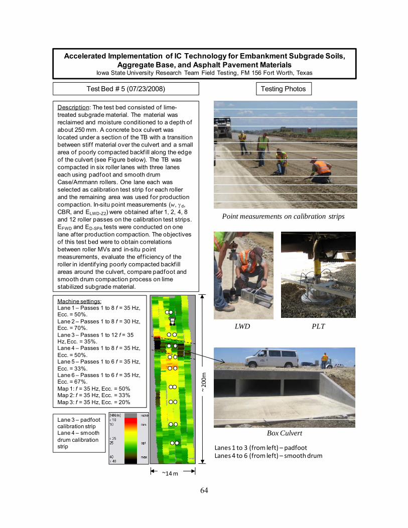
64

Test Bed # 5 (07/23/2008) Testing Photos

Description: The test bed consisted of lime-treated subgrade material. The material was reclaimed and moisture conditioned to a depth of about 250 mm. A concrete box culvert was located under a section of the TB with a transition between stif f material over the culvert and a small area of poorly compacted backf ill along the edge of the culvert (see Figure below). The TB was compacted in six roller lanes with three lanes each using padfoot and smooth drum Case/Ammann rollers. One lane each was selected as calibration test strip for each roller and the remaining area was used for production compaction. In-situ point measurements (w, d, CBR, and ELWD-Z2) were obtained af ter 1, 2, 4, 8 and 12 roller passes on the calibration test strips. EFWD and ED-SPA tests were conducted on one lane af ter production compaction. The objectives of this test bed were to obtain correlations between roller MVs and in-situ point measurements, evaluate the ef f iciency of the roller in identifying poorly compacted backf ill areas around the culvert, compare padfoot and smooth drum compaction process on lime stabilized subgrade material.

Accelerated Implementation of IC Technology for Embankment Subgrade Soils, Aggregate Base, and Asphalt Pavement Materials

Iowa State University Research Team Field Testing, FM 156 Fort Worth, Texas

Machine settings:Lane 1 – Passes 1 to 8 f = 35 Hz, Ecc. = 50%.Lane 2 – Passes 1 to 8 f = 30 Hz, Ecc. = 70%.Lane 3 – Passes 1 to 12 f = 35 Hz, Ecc. = 35%.Lane 4 – Passes 1 to 8 f = 35 Hz, Ecc. = 50%.Lane 5 – Passes 1 to 6 f = 35 Hz, Ecc. = 33%.Lane 6 – Passes 1 to 6 f = 35 Hz, Ecc. = 67%.Map 1: f = 35 Hz, Ecc. = 50%Map 2: f = 35 Hz, Ecc. = 33%Map 3: f = 35 Hz, Ecc. = 20%

~ 200m

Point measurements on calibration strips

LWD PLT

Box Culvert

~14 m

Lanes 1 to 3 (from left) – padfootLanes 4 to 6 (from left) – smooth drum

Lane 3 – padfoot calibration stripLane 4 – smooth drum calibration strip

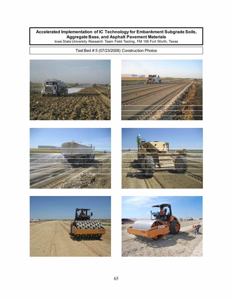
65

Test Bed # 5 (07/23/2008) Construction Photos

Accelerated Implementation of IC Technology for Embankment Subgrade Soils, Aggregate Base, and Asphalt Pavement Materials

Iowa State University Research Team Field Testing, FM 156 Fort Worth, Texas

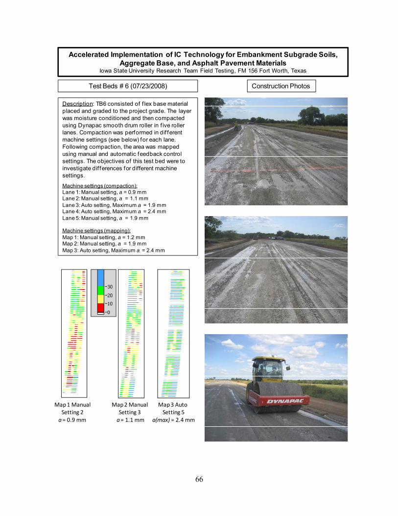
66

Test Beds # 6 (07/23/2008) Construction Photos

Description: TB6 consisted of f lex base material placed and graded to the project grade. The layer was moisture conditioned and then compacted using Dynapac smooth drum roller in f ive roller lanes. Compaction was performed in dif ferent machine settings (see below) for each lane. Following compaction, the area was mapped using manual and automatic feedback control settings. The objectives of this test bed were to investigate dif ferences for different machine settings.

Machine settings (compaction):Lane 1: Manual setting, a = 0.9 mmLane 2: Manual setting, a = 1.1 mmLane 3: Auto setting, Maximum a = 1.9 mmLane 4: Auto setting, Maximum a = 2.4 mmLane 5: Manual setting, a = 1.9 mm

Machine settings (mapping):Map 1: Manual setting, a = 1.2 mmMap 2: Manual setting, a = 1.9 mmMap 3: Auto setting, Maximum a = 2.4 mm

Accelerated Implementation of IC Technology for Embankment Subgrade Soils, Aggregate Base, and Asphalt Pavement Materials

Iowa State University Research Team Field Testing, FM 156 Fort Worth, Texas

Map 3 Auto Setting 5

a(max) = 2.4 mm

Map 2 Manual Setting 3 a = 1.1 mm

Map 1 Manual Setting 2 a = 0.9 mm

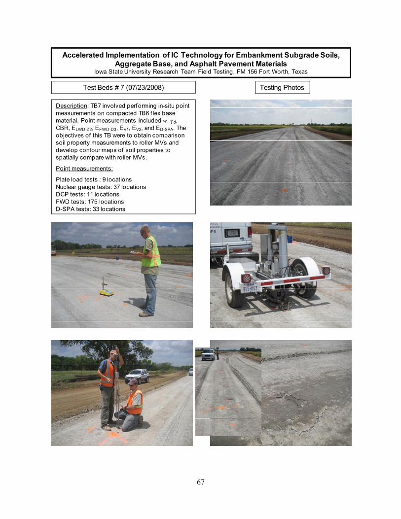
67

Test Beds # 7 (07/23/2008) Testing Photos

Description: TB7 involved performing in-situ point measurements on compacted TB6 f lex base material. Point measurements included w, d, CBR, ELWD-Z2, EFWD-D3, EV1, EV2, and ED-SPA. The objectives of this TB were to obtain comparison soil property measurements to roller MVs and develop contour maps of soil properties to spatially compare with roller MVs.

Point measurements:

Plate load tests : 9 locationsNuclear gauge tests: 37 locationsDCP tests: 11 locationsFWD tests: 175 locationsD-SPA tests: 33 locations

Accelerated Implementation of IC Technology for Embankment Subgrade Soils, Aggregate Base, and Asphalt Pavement Materials

Iowa State University Research Team Field Testing, FM 156 Fort Worth, Texas

Picture of test bed