integration of geodetic and geotechnical deformation surveys in the geosciences
TRANSCRIPT

Tectonophysics. 130 (1986) 369-383
Elsevier Science Publishers B.V., Amsterdam - Printed in The Netherlands
369
INTEGRATION OF GEODETIC AND GEOTECHNICAL DEFORMATION
SURVEYS IN THE GEOSCIENCES
ADAM CHRZANOWSKI, YONGQI CHEN *. PABLO ROMERO and JAMES M. SECORD
Department of Surveying Engineering, Unioersity of New Brunswick, P.O. Box 4400,
Fredericton, N. B. E3B 5A3 (Canada)
(Accepted March 18. 1986)
ABSTRACT
Chrzanowski. A., Chen. Y.Q., Romero. P. and Secord. J.M., 1986. Integration of geodetic and geotechni-
cal deformation surveys in the geosciences. In: H.G. Henneberg (Editor), Recent Crustal Movements.
1985. Tectonophysics, 130: 369-383.
Ground movement studies can utilize information from conventional geodetic surveying. photogram-
metry. and geotechnical measurements of strain, tilt. etc. Each method alone cannot yield a complete
picture of the deformation. However, each is complemented by the others. Hence. their integration in a
simultaneous analysis in space and in time is advocated. An integrated analysis is readily accommodated
by a generalized method of deformation analysis devised by the authors. Any number of measurements
of any type can be considered in any fashion of modelling with full statistical assessment of the
modelling and of derived characteristics. Such an integration is illustrated using data from a coal mining
area in rugged mountainous terrain of western Canada. Conventional terrestrial geodetic methods
connected 15 stations. Displacements from an additional 29 points were obtained from aerial photogram-
metry. Biaxial tiltmeters continuously measured ground tilts at 3 stations. A surface of subsidence for the
whole area was modelled with the graphical depiction in three dimensions.
1. INTRODUCTION
Monitoring surveys in the geosciences, for purposes such as investigations of
tectonic movements, landslides, or natural or man-induced ground subsidence, can
be categorized into three main groups according to the methodology and instrumen-
tation used: geodetic surveying methods; photogrammetric surveys: and geotechni-
cal measurements (using strainmeters, extensometers, tiltmeters, etc.).
Geodetic surveys offer high accuracy in the relative positioning of discrete
monitoring points and give a global picture of the status of deformation. However,
* On leave from the Wuhan Technical University of Surveying and Mapping. Wuhan. P.R. of China.
0040-1951/86,‘$03.50 10 1986 Elsevier Science Publishers B.V

370
they are slow and their adaptation to continuous and automatic monitoring is difficult and expensive.
Photogrammetric surveys provide an instant capture of the deformation status of the whole object of interest, including inaccessible areas, and the field work is relatively light. But their accuracy is not always sufficient.
Geotechnical surveys supply highly accurate information regarding deformation and are easily adaptable for continuous. fully automatic and telemetric data acquisition. In comparison with the two other methods, they are independent of environmental conditions such as snow coverage or poor visibility. However, they provide only local information at discrete points.
Each of the above methods, if used separately, may lead to physical misinterpre- tation of the actual deformation. For example, change in the distances in a geodetic network in a seismically active area may be prematurely interpreted as strain accumulation, while in reality the observed changes could be produced just by rigid body dislocation of the geodetic points due to discontinuities in the deformable object. In this case, the addition of local strain measurements could help in arriving at a proper deformation model.
From the above, one can clearly see that each of the three methods complements the other two. Therefore, an integration of the different methods is recommended.
In practice, one could find many monitoring projects where the data from geotechnical and geodetic measurements have been collected and analysed sep- arately by different specialists without any attempt to integrate or, at least, to exchange the information for a better understanding of the deformation mechanism.
The authors have developed a generalized approach (Chen, 1983; Chrzanowski et al., 1983) to the deformation analysis in which any type of observations measured in several campaigns can be analysed simultaneously in space and time. A summary of the approach is given below together with an example of its application to a ground subsidence study in which geodetic, photogrammetric, and geotechnical measure- ments have been integrated in a simultaneous geometrical analysis.
2. BASIC PRINCIPLE OF THE GENERALIZED APPROACH
The defo~tion of a body is ful.ly described in three dimensions if nine deformation parameters, i.e., six strain and three differential rotation components, can be determined at each point. In addition, components of relative -rigid body motion between blocks should also be determined if discontinuities exist in the body. The above deformation parameters can be easily calculated if a dispfacement function d(x, y, z; t - to) is known (e.g., Sokolnikoff, 1955). Since, in practice, deformation surveys are made only at discrete points, displacement fun&ion must be approximated through some selected model which fits into the observation data in the best possible way.

371
The displacement function can be written in matrix notation as:
~~~,i,;;*-_~I=/,I,IIl::rEl~=~~ (1)
where u, u, u’ are the components of the displacement in the x, _v, z directions,
respectively, B is the deformation matrix with its elements being functions of the
position of the observation points and of time, and c is the vector of unknown
coefficients. A vector Al of changes in any type of observations or quasi-observa-
tions, for instance the coordinates derived from photogrammetric surveys, can be
expressed in terms of the displacement function as:
Al=ABc=& (2)
where A is the transformation matrix (or configuration matrix) relating the observa-
tions to the displacements. In the case of the observations being changes in
coordinates (displacements) of the observed points, the matrix A becomes the
identity matrix. The functional relationship between different types of observables
and coefficient vector c is given in Appendix I.
If redundant observations are made, the elements of the unknown vector c are
estimated through the least-squares approximation:
E = ( bTPA,b) -lBTPA, Al (3)
and have the covariance matrix
ct=fJ;(BTPJj-’ (4)
where PA, is the weight matrix for Al, and ui is the variance factor.
In a more general case, when a simultaneous multi-epoch analysis of the
observables y, (i = 1, 2,. . . , k epochs) is performed, a general solution to the vector
c has been elaborated in Chen (1983) and reads as:
(5)
where Pi is the weight matrix of observations in epoch i.
The above solution takes care of possible datum and configuration defects in the
monitoring network when quasi-observations are involved.
It can be shown that the solution (3) is a special case of the general solution (5)
when only two epochs are considered.
The generalized approach is applicable to any type of geometrical analysis, both
in space and in time, including the detection of an unstable area and the determina-

372
tion of strain components and relative rigid body motion within a deformed object. It allows utilization of different types of surveying data and geotechnical measure- ments. In practical application, the approach consists of three basic processes: identification of deformation models; estimation of the deformation parameters: diagnostic checking of the models and the final selection of the “best” model.
The analysis procedures using the approach can be summarized in the following steps:
Sfep 1. Assessment of the observations using the minimum norm quadratic unbiased estimation (MINQUE) principle to obtain the variances of observations and possible correlations of the observations within one epoch or between epochs, if the a priori values are not available.
Step 2. Separate adjustment of each epoch of geodetic or photogrammetric observations, if such are available, for detection of outliers and systematic errors. If correlations of the observations between epochs are not negligible, then simulta- neous adjustment of multiple epochs of observations is required.
Steps 1 and 2 overlap because the existence of outliers and systematic errors will influence the estimated variances and covariances and the adopted variances and covariances of the observations will affect outlier detection.
Step 3. Comparison of pairs of epochs; selection of deformation models based on a priori considerations and trend analysis from the displacement pattern, if such is available from the observations. If a monitoring network suffers from datum defects, the method of iterative weighted projection (Chen, 1983) is used to yield the “best” picture of the displacement pattern. Examples of typical deformation models are given in Appendix II for illustration.
Step 4. Estimation of the coefficients of deformation models and their covari- antes using all available information.
Step 5. Global test on the deformation model: testing groups of coefficients or an individual one for significance.
The above three steps should be considered as an iterative three-step procedure, so they necessarily overlap.
Step 6. Simultaneous estimation of the coefficients of the deformation model in space and in time if the analysis of pairs of epochs of observations suggests that it is worth doing.
This simultaneous estimation must be performed if the observations are scattered in time. The iterative three-step procedure is still valid. The possible deformation models can be selected either based on a priori considerations or by plotting the observations versus time for trend analysis.
Step 7. Comparison of the models and choice of the “best” model. Since more than one of several possible models could fit the data reasonably well, the “best” model is selected according to the criteria: (a) the model passes the global statistical test at an acceptable probability; (b) if more than one model passes the global test, then the model with the fewest significant coefficients is selected; (c) if the two
373
above criteria cannot be satisfied, then the rationale based on physical grounds and
minimal error of fit is used.
Step 8. Calculation of the desired deformation characteristics and their accuracies
from the parameters of the “best” model.
Step 9. Graphical display of the deformation model.
A detailed description of the above steps can be found in Secord (1984).
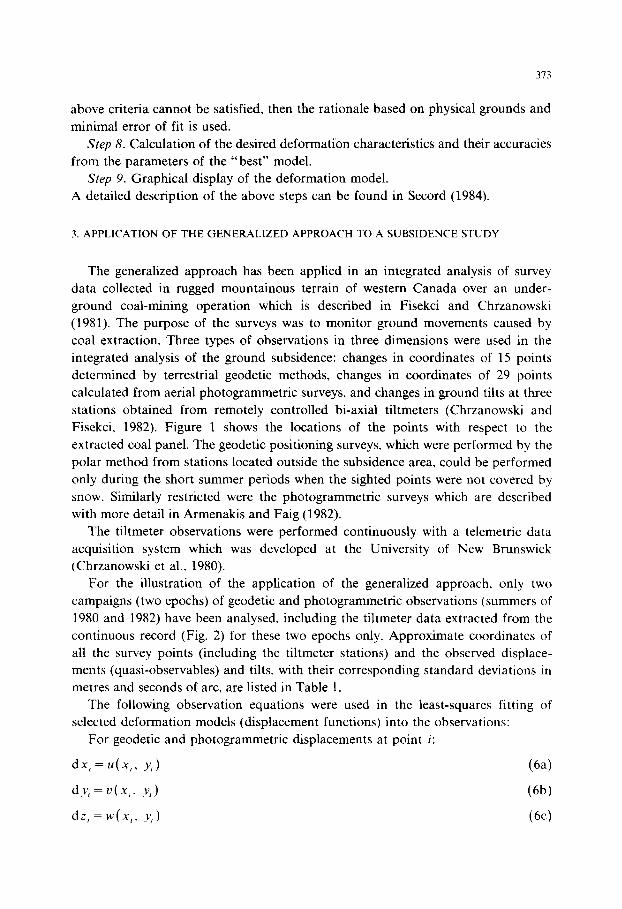
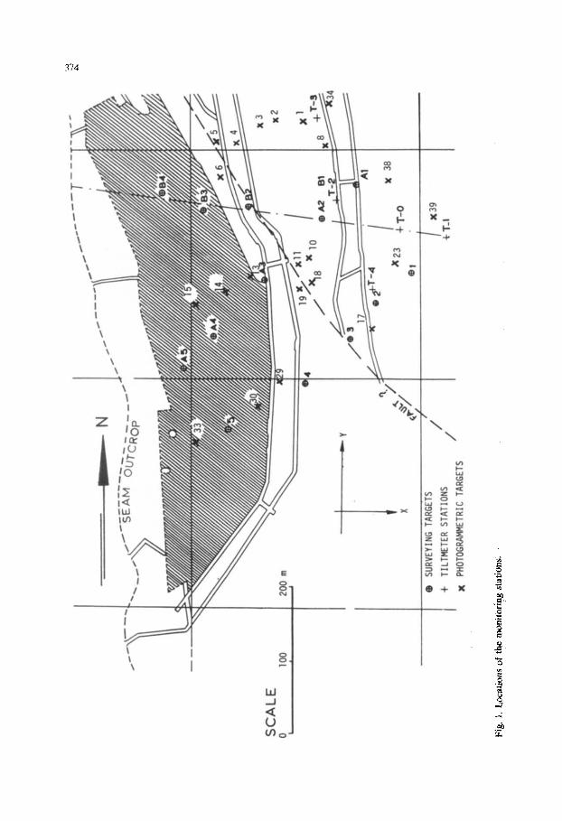
3. APPLICATION OF THE GENERALIZED APPROACH TO A SUBSIDENCE STUDY
The generalized approach has been applied in an integrated analysis of survey
data collected in rugged mountainous terrain of western Canada over an under-
ground coal-mining operation which is described in Fisekci and Chrzanowski
(1981). The purpose of the surveys was to monitor ground movements caused by
coal extraction. Three types of observations in three dimensions were used in the
integrated analysis of the ground subsidence: changes in coordinates of 15 points
determined by terrestrial geodetic methods, changes in coordinates of 29 points
calculated from aerial photogrammetric surveys, and changes in ground tilts at three
stations obtained from remotely controlled bi-axial tiltmeters (Chrzanowski and
Fisekci, 1982). Figure 1 shows the locations of the points with respect to the
extracted coal panel. The geodetic positioning surveys, which were performed by the
polar method from stations located outside the subsidence area, could be performed
only during the short summer periods when the sighted points were not covered by
snow. Similarly restricted were the photogrammetric surveys which are described
with more detail in Armenakis and Faig (1982).
The tiltmeter observations were performed continuously with a telemetric data
acquisition system which was developed at the University of New Brunswick
(Chrzanowski et al., 1980).
For the illustration of the application of the generalized approach, only two
campaigns (two epochs) of geodetic and photogrammetric observations (summers of
1980 and 1982) have been analysed. including the tiltmeter data extracted from the
continuous record (Fig. 2) for these two epochs only. Approximate coordinates of
all the survey points (including the tiltmeter stations) and the observed displace-
ments (quasi-observables) and tilts, with their corresponding standard deviations in
metres and seconds of arc. are listed in Table 1.
The following observation equations were used in the least-squares fitting of
selected deformation models (displacement functions) into the observations:
For geodetic and photogrammetric displacements at point i:
d-x, = u(x,, ~1,) (6a)
d.v, = u(x,. .v,) (6b)
d:, = w(x,, J,) (6~)
374
-X
\ 1

Y

TA
BL
E
1
App
roxi
mat
e co
ordi
nat
es
of m
onit
orin
g st
atio
ns
and
obse
rved
dis
plac
emen
ts
and
tilt
s
App
roxi
mat
e st
atio
n c
oord
inat
es (
m)
Sta
tion
X
/E
Y/N
Z
/H
Dis
plac
emen
t co
mpo
nen
ts
and
thei
r st
anda
rd d
evia
tion
s (m
)
DX
0
DY
0
DZ
Geo
deti
c ob
seru
akw
s
1 0.
000
2 -
41.1
60
4 -
142.
620
5 -
244.
750
Al
- 73
.220
A2
- 11
9.22
0
A3
- 19
5.73
0
A4
- 26
3.62
0
Bl
- 11
9.34
0
B4
- 33
0.82
0
TO
-
14.8
40
Tl
45.8
80
T2
- 98
.870
T3
- 12
4.11
0
T4
- 52
.200
Ph
o~og
rrrm
mer
ric ck
tvat
ion
s
PI
- 14
3.08
4
P2
- 17
5.24
4
P3
- 19
8.63
5
P4
- 22
8.12
6
P5
- 26
0.03
7
0.00
0 19
01.9
20
- 0.
870
0.08
0 -0
.100
0.
080
-0.8
90
- 40
.240
18
61.9
40
- 0.
950
0.08
0 -
0.17
0 0.
080
- 0.
910
- 14
7.94
0 17
53.5
40
- 1.
370
0.08
0 -
0.47
0 0.
080
- 1.
310
-211
.150
16
74.2
60
- 1.
410
0.08
0 -
0.38
0 0.
080
- 1.
730
116.
730
1903
.540
-
1.42
0 0.
080
-0.1
90
0.08
0 -
1.60
0
71.9
10
1862
.010
-
1.61
0 0.
080
- 0.
420
0.08
0 -
1.77
0
- 9.
490
1177
.020
-
1.66
0 0.
080
- 0.
450
0.08
0 -
1.95
0
- 85
.250
17
10.8
40
-1.4
40
0.08
0 -
0.69
0 0.
080
- 1.
550
72.0
10
1862
.120
-
1.51
0 0.
080
- 0.
510
0.08
0 -1
.760
104.
730
1710
.060
-
1.96
0 0.
080
- 0.
670
0.08
0 -
2.18
0
57.6
70
1916
.560
-
1.23
0 0.
080
-0.1
50
0.08
0 -
1.08
0
47.2
20
1935
.960
-
1.12
0 0.
080
- 0.
050
0.08
0 -
0.81
0
96.4
50
1889
.110
-
1.76
0 0.
080
- 0.
460
0.08
0 -
1.57
0
204.
540
1887
.890
-
1.72
0 0.
080
- 0.
460
0.08
0 -
1.42
0
- 22
.400
18
64.1
60
- 1.
070
0.08
0 -
0.25
0 0.
080
-0.9
90
200.
778
1872
.913
-
2.25
0 0.
200
- 0.
380
0.20
0 -
1.04
0
197.
658
1851
.179
-2
.044
I 0.
200
- 0.
610
0.20
0 -1
.960
187.
084
1831
.305
-
1.66
0 0.
200
-0.4
60
0.20
0 -
1.79
0
170.
168
1804
.028
-
0.88
0 0.
200
- 1.
270
0.20
0 -1
.000
169.
388
1784
.374
-1
.800
0.
200
- 0.
690
0.20
0 --
1.5
00
0.15
0
0.15
0
0.15
0
0.15
0
0.15
0
0.15
0
0.15
0
0.15
0
0.15
0
0.15
0
0.15
0
0.15
0
0.15
0
0.15
0
0.15
0
0.30
0
0.30
0
0.30
0
0.30
0
0.30
0

P6
P7
P8
P9
PlO
Pll
P12
P13
P14
P15
PI7
PI8
P19
P21
P22
P23
P24
P29
P30
P31
P34
P36
P38
P39
- 25
3.79
0
- 29
9.97
3
- 11
0.94
4
- 10
9.85
2
- 13
6.99
0
- 15
1.49
2
- 16
9.42
9
- 21
3.25
6
-263
.210
- 29
8.21
3
- 49
.878
- 12
4.96
2
- 14
7.40
2
~ 27
3.26
4
- 23
.818
- 19
.881
- 16
.504
- 17
7.99
0
-211
.152
- 29
9.14
3
- 11
2.57
7
- 69
.030
- 38
.803
42.9
25
Ob
serv
ed r
ilts
(ar
csec
)
TX
128.
100
1769
.042
160.
122
1753
.901
174.
329
1888
.986
77.7
59
1869
.673
44.7
22
1832
.980
36.4
11
1821
.794
16.8
39
1801
.775
- 9.
299
1770
.241
- 20
.368
17
47.9
64
- 43
.793
17
16.9
24
- 57
.124
18
49.8
08
- 15
.079
18
10.6
64
- 34
.829
17
88.6
45
- 94
.973
16
99.6
96
- 16
.468
18
81.7
10
12.8
94
1895
.275
44.0
58
1910
.460
- 15
0.61
1 17
35.8
31
~ 18
3.95
5 17
04.8
84
- 22
5.49
6 16
40.2
57
231.
708
1879
.399
111.
562
1901
.571
129.
198
1910
.744
75.9
02
1940
.332
- 1.
973
- 2.
314
- 1.
461
- 1.
360
- 1.
730
- 1.
820
- 2.
010
- 1.
820
-1.9
40
- 1.
240
- 1.
040
- 1.
700
- 1.
320
- 0.
990
- 1.
210
- 1.
840
- 1.
340
- 1.
710
- 1.
580
- 1.
350
- 1.
190
~ 1.
050
- 1.
360
- 1.
160
0.20
0
0.20
0
0.20
0
0.20
0
0.20
0
0.20
0
0.20
0
0.20
0
0.20
0
0.20
0
0.20
0
0.20
0
0.20
0
0.20
0
0.20
0
0.20
0
0.20
0
0.20
0
0.20
0
0.20
0
0.20
0
0.20
0
0.20
0
0.20
0
~ 0.
700
0.20
0
- 0.
980
0.20
0
- 0.
410
0.20
0
- 0.
567
0.20
0
- 0.
350
0.20
0
- 0.
520
0.20
0
- 0.
160
0.20
0
- 0.
620
0.20
0
- 0.
680
0.20
0
-1.4
40
0.20
0
- 0.
280
0.20
0
- 0.
540
0.20
0
- 0.
590
0.20
0
- 0.
510
0.20
0
- 0.
090
0.20
0
-0.1
28
0.20
0
- 0.
300
0.20
0
- 0.
520
0.20
0
- 0.
430
0.20
0
- 0.
760
0.20
0
- 0.
130
0.20
0
- 0.
200
0.20
0
- 0.
070
0.20
0
- 0.
040
0.20
0
- 1.
750
0.30
0
- 2.
260
0.30
0
- 1.
110
0.30
0
- 1.
650
0.30
0
- 1.
610
0.30
0
- 2.
450
0.30
0
- 2.
140
0.30
0
- 1.
580
0.30
0
- 2.
090
0.30
0
- 1.
510
0.30
0
- 0.
930
0.30
0
- 1.
410
0.30
0
- 1.
020
0.30
0
- 1.
580
0.30
0
- 1.
150
0.30
0
- 1.
510
0.30
0
- 0.
780
0.30
0
~ 0.
680
0.30
0
- 1.
000
0.30
0
- 1.
600
0.30
0
- 1.
020
0.30
0
- 1.
950
0.30
0
- 1.
000
0.30
0
- 0.
780
0.30
0
Tl
2077
.000
30
.000
-
754.
000
30.0
00
T3
2588
.000
30
.000
12
48.0
00
30.0
00
T4
1474
.000
30
.000
-
1105
.000
30
.000

378
For the two components
rx = kw(Xi+ _Yj)
r,, = &W(X,, Y;)
Following the steps of
rY and rV of the tilt observations at a point i:
(7a)
(7b)
the generalized approach, several possible deformation models were fitted to the observations and statistically tested. The following displacement function was finally accepted as the “best” model:
U( x, y) = a, + a,x + a,y + a,xy + qjx*y + asx3 + a,y3 @a)
U(X, y) = 6, + b,y + b,.xy + b4x2 + b,x2y + b,x3 (8b)
w( x, y) = C” + CIX + c,y + c,xy + cqx2 + c,y2 + cgx2y + c,xy2 + (3*x3 (8~)
Table 2 lists the estimated coefficients and their (1 - cw) significances together with the global test of the model. As one can see from the results, all the coefficients are significant at probabilities higher than 87% [(l - a) > 0.871. The significance of 1.000 in the computer output was printed for (1 - CX) > 0.999. The global test passed. Figure 3 shows a computer-generated graphical display of the ground subsidence calculated from the model.
In this particular example, a similar subsidence model would have been obtained when using only geodetic and photogrammetric data without the three tilt stations. However, the continuous record of the tilts suppkl important information on some
TABLE 2
Coefficients of the deformation model and their (1 - a) significances
Coefficients (1 - a)
A0 - 0.9158274408D 00 l.oOoo
BO - 0.185856529OD 00 1.OoOO
co - 0.9706251681D 00 1.0000
Al 0.5136725012D-02 l.OW
A2 - 0.51281899331)-02 l.OooO
A3 - 0,3832308799D-04 0.9975
A6 -O.l184677505D-06 0.9994
A8 -0.3213389714D-07 1.0000
A9 0.3894232203D07 0.9948
B2 O.l523455053D-02 0.9247
B3 O.l997947764D-04 0.9514
Estimated variance factor: 1.2382997605
Degrees of freedom: 102
Chi squared test at 0.05: 0.9580 i 1.0 < 1:6632 ?
Chi squared test at 0.01: 0.8860 < 1.0 < 1.8321 ?
Coefficients (1 - a)
B4 - O.l792043467D-04 0.9999
B6 0.4364056549D-07 0.8767
B8 - 0,4143482424D-07 0.9943
Cl 0.9933722003D-02 1.0000
c2 - 0.668839749OD02 l.OQOO
c3 - 0.7137434691D-04 1.0000
c4 0.3884618663D-04 1.0000
c5 0.5845810260D-04 1.0000
C6 -0.2332744889D.06 1.0000
c7 0.3245244405D-06 l.OWO
C8 0,2888329518D-07 1.0000

319
3x0
abrupt changes in the movements of rock masses which can be seen on the display in Fig. 2 and which would have not been noticed without those observations. Detailed discussion on the subsidence interpretation in this example has been considered as being beyond the scope of this paper.
4. CONCLUSIONS
Integration of different types of observables is very important for a proper physical interpretation and better understanding of the deformation phenomena. In the geosciences, when the deformation studies extend over large areas, for instance, in investigation of earth crustal movements, an integration of space surveying techniques (e.g., GPS, VLBI) with micro-measurements (micro-geodetic and geo- technical) of the stability of the observing stations should be made. The generalized approach provides a tool for such analysis.
The example of the ground subsidence study in which the 3-D geodetic, photo- grammetric, and tilt measurements have been integrated in the geometrical analysis demonstrates the flexibility of the approach.
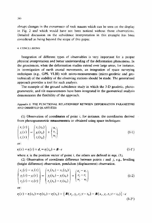
Appendix I: THE FUNCTIONAL RELATIONSHIP BETWEEN DEFORh4ATION PARAMETERS
AND OBSERVED QUANTITIES
(1) Observation of coo~climtes of point i, for instance, the coordinates derived from photogrammetric measurements or obtained using space techniques:
(1-l)
~(l)=~(t)+d,=r;(to)+B.c (I-l’)
where 4 is the position vector of point i, the others are defined in eqn. (1). (2) Observation of coordinate difference between points i and j, e.g., levelling
(height difference) observation, pendulum (displacement) observation.
l+(t) -x,(t) ’
Y;(t) -Y,(f) = (I-2)
\ zjw -G(t)
or:

381
(3) Observation of azimuth from point i to point j:
q(t) =‘Y,,(f0) + - i
cos a,J sin arj u/ - u,
s,, cos p,, ’ s,, cos p,, H 1 . v, - I,, (I-3)
where /3,, and S,, are the vertical angle and spatial distance from point i to point j,
respectively.
The observation of a horizontal angle is expressed as the difference of two
azimuths.
(4) Observation of the distance between point i and point j:
u, - u,
S,,(t) = S,,( t,,) + (cos /?,, sin (Y,,, cos p,, cos (Y,,, sin p,,) .
1 1
5 - L’, (I-4) M; - W,
(5) Observation of strain along the azimuth (Y and vertical angle p at point i:
+)=c(t,)+PTEP (I-5)
where PT = (cos p sin OL, cos /3 cos LX, sin /?) and:
i au au au - - - ax av aZ
at) aLI au - - - E = ax ay aZ
au, aw awl --- , ax ay a,-
,
(6) Observation of a vertical angle at point i to point j:
(
sin J3,j sin (Y,, sin j?,, cos (Y,, cos P,, u, - u,
P,,(r)=P,,(Gl)+ - s 9- s v, - D,
1.1 IJ u; - w,
(7) Observation of a horizontal tiltmeter:
aw a u’ ~(t)=~(t”)+- sina+- coscu
ax al (I-7)
where (Y is the orientation of the tiltmeter.
Appendix II: SOME TYPICAL DEFORMATION MODELS (Chrzanowski et al.. 1982)
(1) Single point displacement or a rigid body displacement (Fig. 4a) of a group of
points (say block B) with respect to a stable block (say block A); the deformation
model is:
uA(x. _r)=O. P,(x, y)=O, u~(.x, .~)=a, and L~~(x, y)=b, (11-l )

3x2
L-----+X
fa) IhJ
Fig. 4. Typical deformation models.
(2) Homogeneous strain (Fig. 4b) in the whole body without discontinuities; For the whole body, the linear deformation model is:
u( x, y) = a,x + a,y and u(x, .v) = b,x + b,y (11-2)
which, after using the well-known infinitesimal strain displacement relationships, becomes:
U( x, y) = ex. x + c’x” ‘_V - wy (11-3)
u(x, y)=f,,..x+e;y+wx (II-4)
where:
(3) A deformable body with one discontinuity, say between blocks A and B, with different linear deformations of each block plus a rigid body displacement of B with respect to A (Fig. 4c):
u.,#( x, y) = a,x -I- a,_Y (II-5)
uA(x, Y) = b,x + b,v (11-6)
UB(X, r> = co + crx + c2y (11-7)
%(X1 Y) = go + t?lX + g2Y (11-8)
In the above case, components Aui and Au, of a total relative dislocation at any point i located on the discontinuity line between blocks A and B may be calculated as:
Aui=uB(Xi, Y~)-uA(X~, ~8) (II-9)
and:
Aui 5 ug(xi? ~1) - uA(Xi, ~1) (II-lo)

383
Usually. the actual deformation model is a combination of the above simple
models or, if more complicated, it is expressed by non-linear displacement functions
which require fitting of higher order polynomials or other suitable functions.
If time-dependent deformation parameters are sought then the above deforma-
tion models will contain a time variable. For instance. in the first model above, if
the velocity (rate) and acceleration of the dislocation of block B in respect to block
A are to be found, the deformation model would be:
u,~ = 0. ~1~ = 0, us = ci,t + Zi,t’ and us = &,t + &,t’ (11-11)
and, in the model of the homogeneous strain, if a linear time dependence is
assumed. the model becomes:
u(x. x. t) = i,xt + i,,.yt - cjyt (H-12)
u(x, _V. t)=I,,.xt+i,.yt+cjxt (H-13)
where the dot above the parameters indicates their rate (velocity) and the double
dot, acceleration.
REFERENCES
Armenakis, C. and Faig, W. 1982. Subsidence monitoring by photogrammetry. Proc. 4th Can. Symp. on
Mining Surveying and Deformation Measurements, Banff. pp. 197-208.
Chen. Y.Q., 1983. Analysis of Deformation Surveys-A Generalized Method. Dep. Surv. Eng. Tech.
Rep. 94. Univ. New Brunswick. Fredericton. N.B.
Chrzanowski. A. and Fisekci, M.Y., 1982. Application of tiltmeters with a remote data acquisition in
monitoring mining subsidence. Proc. 4th Can. Symp. on Mining Surveying and Deformation Surveys,
Banff. pp. 321-333.
Chrzanowski. A., Faig, W.. Kurz, B.J. and Makosinski. A.. 1980. Development, installation and operation
of a subsidence monitoring and telemetry system. Final report to the Canada Centre for Mineral and
Energy Technology, Calgary.
Chrzanowski. A.. Chen, Y.Q. and Secord, J.M.. 1983. On the strain analysis of tectonic movements using
fault-crossing micro-geodetic surveys. Tectonophysics. 97: 297-315.
Fisekci. M.Y. and Chrzanowski, A., 1981. Some aspects of subsidence monitoring in difficult terrain and
climate conditions of Rocky Mountains, western Canada. In: S. Peng (Editor). Proc. Workshop on
Surface Subsidence due to Underground Mining, Morgantown. WV, University of West Virginia. pp.
1822197.
Secord. J.M.. 1984. Implementation of a generalized method for the analysis of deformation surveys.
M.Sc.E. thesis. Department of Surveying Engineering. University of New Brunswick. Fredericton.
N.B.
Sokolnikoff. IS.. 1956. Mathematical Theory of Elasticity. McGraw-Hill. New York.