integrating landscape connectivity and habitat suitability to guide

Integrating landscape connectivity and habitat

suitability to guide offensive and defensive invasive

species management

Ben Stewart-Koster1*, Julian D. Olden1 and Pieter T. J. Johnson2

1School of Aquatic and Fishery Sciences, University of Washington, Seattle, WA, USA; and 2University of Colorado,

Boulder, CO, USA

Summary

1. Preventing the arrival of invasive species is the most effective way of controlling their

impact. Preventative strategies may be ‘offensive’ aimed at preventing the invader leaving col-

onised locations or ‘defensive’ aimed at preventing its arrival at uninvaded locations. The lim-

ited resources for invasive species control must be prioritized, particularly for numerous

vulnerable locations or uncertainty about which sites are already invaded.

2. We developed an integrative modelling framework to prioritise locations for either strategy

by incorporating connectivity and habitat suitability. We applied this framework to a data set

comprising 5189 water bodies in Wisconsin and Michigan, U.S.A, for zebra mussels Dreissena

polymorpha and Eurasian watermilfoil Myriophyllum spicatum. We developed the framework

with a spatial graph based on recreational boater movement and habitat suitability models.

3. An historical graph comprised 3105 natural lakes connected in one of 18 components,

whereas a total of 3944 water bodies (lakes and reservoirs) were connected in one of 13 sepa-

rate components in a graph of the contemporary system. Habitat suitability models accounted

for around half of the deviance in the distribution data for each species.

4. There was a distinct spatial pattern in the levels of risk and subsequent recommended alloca-

tion of management interventions across several levels of investment. Higher risk water bodies

were generally found in the largest component of the spatial graph. At comparatively low levels

of investment, where managers target 5% of all locales to control D. polymorpha, the results

suggested that 71% and 27% of this effort should be committed to defensive and offensive strat-

egies, respectively, in the largest component. For M. spicatum, 92% and 8% of this effort

should be allocated in this component to defensive and offensive strategies, respectively. It is

only with much greater investment that water bodies in other components should be targeted.

5. Synthesis and applications. Allocating limited resources to prevent the spread of invasive

species is a challenge that transcends ecosystems and geography. We successfully identified a

reduced number of locations to target for offensive and defensive intervention strategies for

two species. This framework is readily applicable to other aquatic and terrestrial ecosystems

vulnerable to invasive species.

Key-words: connectivity, Eurasian watermilfoil, generalised additive models, graph theory,

invasive species management, risk assessment, spatial graph, zebra mussels

Introduction

Mounting theoretical and empirical research has revealed

numerous challenges to modelling pathways that might

promote invasive species (Hastings et al. 2005; Wilson et al.

2009) while illustrating the opportunity for this knowledge

to inform management strategies (Vander Zanden & Olden

2008; Hulme 2009). Accordingly, the prevention of initial

invasions is now a clear priority in emerging management

policies (Lodge et al. 2006; Hulme et al. 2008). Attempts

to prevent the secondary spread of an established invasive

species, however, are complicated by the landscape con-

*Correspondence author. Griffith University, Australian Rivers

Institute, 170 Kessels Road, Nathan, QLD 4111, Australia.

E-mail: [email protected]

© 2015 The Authors. Journal of Applied Ecology © 2015 British Ecological Society

Journal of Applied Ecology 2015, 52, 366–378 doi: 10.1111/1365-2664.12395

text of vulnerable habitats and what may be arbitrary

management jurisdictions – the so-called ‘management

mosaic’ (Epanchin-Niell et al. 2010). As contemporary

landscapes are managed for a variety of uses and out-

comes, effective local-scale prevention measures can be

undermined by lack of action at neighbouring source hab-

itats (Peters & Lodge 2009), particularly when such source

habitats occur in a separate management district. This chal-

lenge is particularly acute in fragmented or patchy environ-

ments where the natural and human-mediated connectivity

may have changed over both space and time (von der Lippe

& Kowarik 2007; Fausch et al. 2009; Rahel 2013).

Strategies for the prevention of secondary spread in

patchy environments can broadly be considered as either

offensive or defensive (Drury & Rothlisberger 2008).

Offensive strategies aim to contain potential invaders at

source locations, whereas defensive strategies aim to pre-

vent the arrival at currently uninvaded locations. It

remains a challenge to identify the most effective location

and scale at which to apply these preventive measures;

each strategy might be required depending on the suitabil-

ity of the habitat to the invader (target defensive) or the

probability of dispersal from an invaded site (target offen-

sive). Simulation models support the intuitive prediction

that defensive strategies are likely to be more effective

once more than half of the habitats are invaded (Drury &

Rothlisberger 2008). However, where invasive species

management is coordinated at a regional scale and

includes hundreds or even thousands of locales, often with

imperfect knowledge of invasive species distributions, such

general findings may be difficult to implement. A multi-

scale approach that incorporates the functional connectiv-

ity of the entire system with the suitability to potential

invaders of specific locations would represent an impor-

tant step in addressing this challenge.

Graph-theoretical methods have received growing atten-

tion in ecological applications as a way to visualise and

quantify connections between habitat nodes in space

(Dale & Fortin 2010). A spatial graph consists of nodes –representing habitat patches – that may be connected by

arcs or links that depict pathways of potential for move-

ment of a focal species, genes or populations (Urban &

Keitt 2001; Galpern, Manseau & Fall 2011; Er}os et al.

2012). Links within a graph may be binary, indicating the

presence of a connection or quantitative, representing

actual distance or the probability of connectivity between

two nodes (Dale & Fortin 2010). Analyses of the topology

of a graph provide insight into the connectivity of the

landscape under study (Galpern, Manseau & Fall 2011;

Er}os et al. 2012). Additionally, there is capacity to incor-

porate the habitat quality of each location to weight the

nodes of the graph, either explicitly or implicitly (Dale &

Fortin 2010). In the context of invasive species manage-

ment, such information may provide a way to identify

specific habitats as well as broader regions that would be

most suitable for offensive or defensive strategies. The

value of this type of analysis may be enhanced when

combined with habitat suitability modelling to allow con-

current analysis of the probability of arrival and establish-

ment of invasive species in new locales.

Recent years have seen ecologists combine multiple

models into integrative frameworks to model and forecast

invasive species distributions and for risk assessment

(Franklin 2010; Ib�a~nez et al. 2014). These approaches typi-

cally include empirical or phenomenological models, such

as gravity models, spatial statistical models or machine

learning methods (Leung & Mandrak 2007; Vander Zanden

& Olden 2008; Rothlisberger & Lodge 2009), which may

be coupled with dynamic population models (Franklin

2010; Gallien et al. 2010). Although there are many

advantages to these approaches, the use of dynamic

population models may only be feasible when life-history

parameters and specific habitat requirements are well

understood (Keith et al. 2008; Ib�a~nez et al. 2014).

Dispersal events by invaders are often highly stochastic;

therefore, it can be difficult to define dispersal parameters

and thus accurately predict colonisation (Rothlisberger &

Lodge 2009). In the absence of suitable data to estimate

such parameters, quantifying the different axes of invasion

risk with empirical models may offer a way forward when

urgent management interventions are required.

The aim of this study was to develop an integrative

modelling framework that effectively operationalized the

concepts of offensive and defensive management strategies

for invasive species management. To quantify where and

how to prioritise these strategies, we developed a risk met-

ric based on emerging graph-theoretical techniques and

habitat suitability models. This metric simultaneously

integrated the effects of habitat quality, spatial proximity

and the probable connectivity of each potential locale.

Importantly, our approach provides an avenue to make

recommendations for interventions at both local and land-

scape scales. To demonstrate the utility of this approach,

we examined the diverse freshwater landscapes of the

mid-western United States, which has a high concentra-

tion of both natural lakes and artificial reservoirs that

have been invaded by numerous non-native species (Van-

der Zanden & Olden 2008). Lake systems are exemplary

of fragmented landscapes with suitable habitats nested

within a broader habitat matrix that is unavailable to resi-

dent biota, best illustrated by the ‘lakes-as-islands’ anal-

ogy (Keddy 1976; Arnott et al. 2006). Today, water

bodies in the region are invaded by species such as zebra

mussels Dreissena polymorpha and Eurasian watermilfoil

Myriophyllum spicatum, two highly invasive species with

respect to ecological and economic impacts (Johnson,

Olden & Vander Zanden 2008).

Materials and methods

STUDY REGION AND SPECIES

We compiled species and environmental data for 5189 water

bodies representing 4183 lakes and 1006 reservoirs (≥0�04 km2 in

© 2015 The Authors. Journal of Applied Ecology © 2015 British Ecological Society, Journal of Applied Ecology, 52, 366–378

Prioritising invasive species management 367

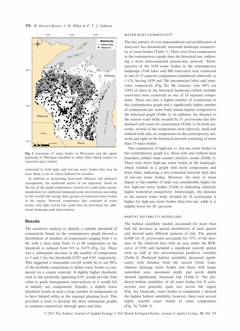
surface area and ≥2 m in maximum depth) distributed across

Wisconsin and the upper peninsula of Michigan, U.S.A (Fig. 1;

Johnson, Olden & Vander Zanden 2008). Historical connectivity

in this system is a function of lake hydrology, with drainage lakes

having clear movement corridors along stream channels and the

many seepage lakes being historically disconnected. However,

contemporary connectivity is also influenced by human activity;

the construction of artificial reservoirs has created barriers to in-

channel movement (Johnson, Olden & Vander Zanden 2008),

whereas the entrainment of invasive species on recreational boat-

ing and fishing equipment (so-called ‘hitchhiking’) has facilitated

the overland dispersal of many species (Johnson & Carlton 1996;

Buchan & Padilla 1999). We broadly classified reservoirs to

include hydroelectric reservoirs, impoundments created by dam-

ming a river or flooding a low-lying area, lakes equipped with

stabilizing dams or created through soil excavation, and mill, irri-

gation or stock ponds.

Occurrence of D. polymorpha and M. spicatum was obtained

from the Wisconsin Department of Natural Resources (WDNR),

Michigan Department of Environmental Quality (MDEQ), the

Great Lakes Indian Fish & Wildlife Commission (GLIFWC) and

the Center for Limnology at University of Wisconsin (CFLUW)

according to strict inclusion criteria (see Johnson, Olden & Van-

der Zanden 2008). Distributional data were collected primarily

during broad-scale field surveys, rather than through isolated

accounts, thereby reducing the likelihood of any systematic biases

in the data. Environmental characteristics used for habitat suit-

ability modelling were obtained from the WDNR Register of

Waterbodies, the Wisconsin Lakes Book, the Surface Waters of

Wisconsin volumes and the MDEQ.

Dreissena polymorpha are relatively small (25–35 mm length)

suspension-feeding mussels that commonly reach densities exceed-

ing 10 000 individuals m�2 (Berkman et al. 1998). Dreissena poly-

morpha can dramatically affect phytoplankton abundance,

nutrient cycling and water clarity and are associated with declines

in native biota (Higgins & Vander Zanden 2010) as well as signifi-

cant economic damages via fouling and water treatment (Connelly

et al. 2007). The invasion of D. polymorpha into North America

was facilitated through the ballast water of trans-Atlantic ships

and was first identified in the western basin of Lake Erie during

1986 (Carlton 2008). Within a few years of establishment, D. poly-

morpha expanded its range to include all five of the Laurentian

Great Lakes, reached the upper Mississippi River by 1991, and

currently has expanded its range southward to the Gulf of Mexico

(Benson 2013). Secondary spread of D. polymorpha has been lar-

gely facilitated by entrainment on recreational boats by encrusting

on hulls and entanglement on engine propellers and fishing equip-

ment (Rothlisberger et al. 2010). Data used in our analysis

included verified reports of established adult populations, standar-

dised visual and substrate sampling by the WDNR and veliger

larvae sampling by the WDNR (1998–2006) and GLIFWC (2003-

2006). Briefly, veliger sampling involved epilimnetic vertical tows

of a 50–64 micron mesh zooplankton net (50 cm opening) per-

formed at three sites per water body and on three different dates

during the summer season (late June to August). Preserved sam-

ples were subsequently examined for the presence of Dreissena

veliger larvae (Johnson, Olden & Vander Zanden 2008).

Myriophyllum spicatum was first introduced to the United

States in the 1940s and presently occupies 46 states and several

Canadian provinces from Qu�ebec to British Columbia (Moody &

Les 2007). Initially introduced accidentally via the plant aquarium

trade, human transport of plant fragments on boating equipment

is now cited as the most important vector of dispersal among

water bodies for M. spicatum (Madsen & Smith 1997; Rothlisber-

ger et al. 2010). This species is a perennial herbaceous submersed

plant, which forms a dense canopy of branches, and causes

marked changes in macrophyte cover, light penetration, nutrient

cycling and invertebrate and vertebrate communities (Smith &

Barko 1990). Myriophyllum spicatum was first found in south-

eastern Wisconsin in the mid-1960s and has since spread north-

ward and westward. Distribution data for M. spicatum in

Wisconsin and Upper Peninsula Michigan came from surveys

conducted by the WDNR (and its volunteer monitoring

programme), GLIFWC and CFLUW. We relied heavily on

broad-scale survey data collected by Stanley Nichols and col-

leagues between 1976 and 2000 (Nichols & Martin 1990). Sam-

pling methodologies involved a fixed number of rake throws

along transects in the littoral zone (http://lter.limnology.wisc.edu/

protocols.html).

SPATIAL GRAPHS

As the principal vector of dispersal of invasive species in this sys-

tem is entrainment on recreational boating equipment, we devel-

oped a spatial graph for the 5189 water bodies (i.e. graph nodes)

with links derived from a probability of connectivity via road tra-

vel. Recent surveys suggest that up to 30% of recreational boat-

ers in the region seldom or never wash down their equipment

after use, while 32% may at times travel directly between lakes

on the same day (Peterson & Nelson 2008). Nonetheless, the

majority of boat users visit one water body per trip (Buchan &

Padilla 1999), which means that most hitchhiking propagules are

not transported directly from one water body to another. Rather,

potential introductions most likely occur on subsequent trips to

uninvaded water bodies within a time frame that propagules

remain viable. To accommodate this, we used the centroid of

each county in the region as a surrogate for boaters’ residences

(given that boater’ addresses were not collected) and routed all

road distances through these locations.

We began by generating a matrix of road distances between

each water body and all of the county centroids. We then con-

verted these road distances to probabilities based on an empirical

distribution of boater travel in Wisconsin, which was highly cor-

related with the observed pattern of spread of D. polymorpha

(Buchan & Padilla 1999). This provided an estimate of the proba-

bility of travel to each water body from each of the county cent-

roids in the region. We used these probabilities to derive a

probability of connectivity between each pair of water bodies.

For a pair of water bodies in the same county, the probability of

connectivity was simply the product of the probability of travel

from the centroid to each water body. For a pair of water bodies

in different counties (lake 1 in county A and lake 2 in county B),

we calculated two estimates of the probability of connectivity: the

first of these being the product of the probability of travel from

each lake to the centroid of county A and the second being the

product of the probability of travel from each lake to the

centroid of county B. We set the probability of connectivity

between the two lakes as the maximum of these two values. This

resulted in a pairwise matrix of probabilities of connectivity

among all water bodies in the data set from which we built a

contemporary spatial graph using all water bodies including

artificial reservoirs. We subsequently identified the proportion of


368 B. Stewart-Koster, J. D. Olden & P. T. J. Johnson

http://lter.limnology.wisc.edu/protocols.html

http://lter.limnology.wisc.edu/protocols.html

probable connections to define two water bodies as ‘connected’

via a sensitivity analysis that varied the possible threshold

between 0�025 and 0�975.Having determined a set of pairwise connections using the con-

temporary spatial graph, we constructed three additional graphs:

(i) an historical graph represented by only natural lakes; (ii) a

contemporary high-use graph representing only water bodies with

boat launches and (iii) a contemporary low-use graph represent-

ing only water bodies without boat launches. This enabled us to

evaluate the effect of the relatively recent construction of artificial

reservoirs on the connectivity of the system, assuming contempo-

rary boater movements, and examine the potential vulnerabilities

in the system at high-use water bodies.

To assess network topology and quantify different elements of

connectivity, we computed a series of graph-theoretical indices

for each graph. First, we calculated the number of components

to quantify the connectivity of the spatial graphs as a whole. A

component is a set of nodes (here, water bodies) in which there is

a path, though not necessarily a direct link, between all pairs of

nodes (Galpern, Manseau & Fall 2011). As such, all components

are effectively disconnected from each other (Pascual-Hortal &

Saura 2006) and could be used as discrete management units to

guide local and landscape scale invasive species interventions. As

the connectivity of the entire graph increases, the number of com-

ponents decreases. Second, we computed the number of links in

each graph. At the water body level, we computed the node

degree for each water body, which is the number of binary con-

nections of that node. As the connectivity of a node increases, so

does its degree. Third, we calculated the mean distance to an

invaded water body in each graph. We calculated the number of

components using Conefor Sensinode 2.2 (Saura & Torn�e 2009),

while all other graph-theoretical indices were calculated in the R

statistical environment version 2.14.1 (R Development Core

Team 2012).

HABITAT SUITABIL ITY MODELLING

For each water body, we estimated the suitability of habitat for

D. polymorpha and M. spicatum by fitting logistic generalised

additive models (GAMs) using presence/absence data from a sub-

set of the water bodies (n = 312 for D. polymorpha and n = 601

for M. spicatum). Generalised additive models are a flexible non-

parametric approach to regression modelling that can account for

nonlinear relationships via the use of splines (Hastie & Tibshirani

1990). The spatial GAMs were fit with a set of predictor variables

and a smoothed spatial term, using splines on latitude and longi-

tude, to account for residual spatial variation (Bivand, Pebesma

& G�omez-Rubio 2008). The predictor variables included environ-

mental characteristics deemed important for colonisation and

establishment based on previous investigations (reviewed in John-

son, Olden & Vander Zanden 2008), including maximum depth

(m), surface area (km2), conductance (lmhos cm�1), secchi depth

(m), upstream watershed area (km2), water body type (seepage or

drainage), impoundment status (lake or reservoir), number of

boat launches and the straight line distance to the nearest Great

Lake (either Lake Michigan or Lake Huron). Predictor variables

were selected using backwards elimination to remove statistically

nonsignificant variables while minimising the AIC. The smooth-

ness of the spatial spline was determined by minimising the unbi-

ased risk estimator criterion (Wood 2011). The spatial GAMs

were fit in the R statistical environment (R Development Core

Team 2012) using the mgcv package (Wood 2011). We calculated

the area under the receiver operating characteristic (ROC) curve

using the pROC package (Robin et al. 2011).

MANAGEMENT RECOMMENDATIONS

We combined the results of the GAMs with results of the spatial

graphs to rank water bodies according to priority for manage-

ment intervention relative to other water bodies on a continuous

scale. First, each water body was identified as suitable for offen-

sive or defensive strategies depending on its invasion status and

subsequently prioritised according to a probabilistic estimate of

risk based on combined connectivity and habitat suitability. We

defined the risk of invasion at any given water body as a product

of its habitat suitability and those to which it is connected and its

probable connectivity to other invaded or vulnerable water

bodies:

Ri ¼ Hi �Xj

j¼1

ðHjCijÞ

where Ri is the estimated risk at the ith lake, Hi is the estimated

habitat suitability of the ith lake and Hj is the habitat suitability

of each of the j connected lakes, and Cij is the probability of con-

nection between the ith lake and all j lakes within the component.

For lakes known to be invaded, we simply replaced the model-

estimated habitat suitability Hi or Hj with 1. We used the compo-

nents that were identified in the contemporary spatial graph to

define a neighbourhood for each water body that provided the

connections used to estimate our metric of risk. However, we

used to the probabilistic connections to define Cij, rather than the

binary ones used to define the neighbourhood, which we scaled

within each component to a unit sum. Thus, the sum of all Cij in

each component was 1, which ensured the estimate of risk, Ri,

represented a probability that ranged from 0 to 1.

Under this model, the risk associated with known invaded

water bodies can be interpreted as an offensive risk, and for

water bodies that are uninvaded or unknown, it can be inter-

preted as the defensive risk. We tested the risk metric by evaluat-

ing its capacity as a classifier of invasion status using the area

under the receiver operating characteristic curve (AUC). An

AUC of 1 indicates perfect classification, while an AUC of 0�5indicates no better than random classification (Fielding & Bell

1997). We compared the AUC for the risk metric with that of the

spatial GAMs to assess the improvement in classification when

combining connectivity with habitat suitability.

We prioritised local-scale measures under different budget con-

straints, or levels of investment, according to the spatial distribu-

tion of risk across the components. We quantified different levels

of investment in terms of the proportion of all water bodies at

which intervention measures could afford to be deployed. At each

level of investment, we allocated effort by ranking the water

bodies by their risk and attributing effort accordingly. For exam-

ple, if only 5% of the water bodies in the region could be tar-

geted with a prevention measure, we identified the proportion of

the water bodies above the 95th percentile of risk that fell in each

component. These proportions identified the specific water bodies

to be targeted and by extension the allocation of effort for that

component. An additional step examining high-use water bodies

within the contemporary graph offers a further filter to assist pri-

oritisation. This would identify potential habitats that are highly



connected to both high- and low-use water bodies that may be

more likely to act as source habitats for invaders.

In addition to prioritising local-scale offensive and defensive

management, the multiscale nature of our approach, based on

the use of the graph components, ensured we could make recom-

mendations for additional landscape-scale interventions according

to the overall risk among these groups of connected water bodies

in the region. Network components that consisted of water

bodies with high overall risk could then be prioritised for addi-

tional landscape-scale interventions.

Results

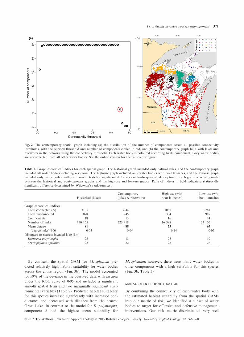
The sensitivity analysis to identify a suitable threshold of

connectivity based on the contemporary graph showed a

distribution of numbers of components ranging from 1 to

60, with a clear jump from 13 to 60 components as the

threshold is reduced from 0�9 to 0�875 (Fig. 2a). There

was a subsequent decrease in the number of components

to 3 and 1 for the thresholds 0�925 and 0�95, respectively.This suggested a reasonable cut-off would be to use 90%

of the probable connections to define water bodies as con-

nected via a county centroid. A slightly higher threshold,

such as the intuitively appealing 0�95, would provide little

value to guide management interventions as it would fail

to identify any components. Equally, a slightly lower

threshold results in such a large number of components as

to have limited utility at the regional planning level. This

provided a basis to develop the three subsequent graphs

to compare connectivity through space and time.

WATER BODY CONNECTIV ITY

The last century of river impoundment and proliferation of

reservoirs has dramatically increased landscape connectiv-

ity of water bodies (Table 1). There were fewer components

in the contemporary graph than the historical one, indicat-

ing a more interconnected present-day network. Three-

quarters of the 5189 water bodies in the contemporary

landscape (3144 lakes and 800 reservoirs) were connected

in one of 13 separate components (numbered arbitrarily as

1–13), leaving 1039 and 206 unconnected lakes and reser-

voirs, respectively (Fig. 2b). By contrast, only 60% (or

3105) of lakes in the historical landscape (which excludes

reservoirs) were connected in one of 18 separate compo-

nents. There was also a higher number of connections in

the contemporary graph and a significantly higher number

of connections per water body (mean degree) compared to

the historical graph (Table 1). In addition, the distance to

the nearest water body invaded by D. polymorpha has also

declined with reservoir construction (Table 1). In both net-

works, several of the components were relatively small and

isolated with only six components in the contemporary net-

work and eight in the historical network consisting of more

than 15 water bodies.

The comparison of high-use vs. low-use water bodies in

the contemporary graph (i.e. those with and without boat

launches) yielded some counter intuitive results (Table 1).

There were fewer high-use water bodies in the landscape,

which resulted in a graph with more components and

fewer links, indicating a less-connected network than that

of low-use water bodies. However, the ratio of mean

degree to the number of links was considerably higher for

low high-use water bodies (Table 1) indicating relatively

higher node-level connectivity. Interestingly, the distance

to the nearest water body invaded by D. polymorpha is

higher for high-use water bodies than low-use, while it is

slightly lower for M. spicatum.

HABITAT SUITABIL ITY MODELL ING

The habitat suitability models accounted for more than

half the deviance in spatial distribution of each species

and showed quite different patterns of risk. The spatial

GAM for D. polymorpha accounted for 53% of the devi-

ance in the observed data with an area under the ROC

curve of 0�94 and included a significant smooth spatial

term as well as five environmental predictor variables

(Table 2). Predicted habitat suitability decreased signifi-

cantly with distance from the nearest Great Lake,

whereas drainage water bodies and those with larger

watershed area, maximum depth and secchi depth

showed significantly increased risk (Table 2). The pre-

dicted habitat suitability of all water bodies for D. poly-

morpha was generally quite low across the region

(Fig. 3a). Generally, water bodies in component 1 showed

the highest habitat suitability; however, there were several

highly suitable water bodies in other components

(Fig. 3a; Table 3).

Fig. 1. Locations of water bodies in Wisconsin and the upper

peninsula of Michigan classified as either lakes (black circles) or

reservoirs (grey circles).



By contrast, the spatial GAM for M. spicatum pre-

dicted relatively high habitat suitability for water bodies

across the entire region (Fig. 3b). The model accounted

for 59% of the deviance in the observed data with an area

under the ROC curve of 0�95 and included a significant

smooth spatial term and two marginally significant envi-

ronmental variables (Table 2). Predicted habitat suitability

for this species increased significantly with increased con-

ductance and decreased with distance from the nearest

Great Lake. In contrast to the model for D. polymorpha,

component 8 had the highest mean suitability for

M. spicatum; however, there were many water bodies in

other components with a high suitability for this species

(Fig. 3b, Table 3).

MANAGEMENT PRIORIT ISATION

By combining the connectivity of each water body with

the estimated habitat suitability from the spatial GAMs

into our metric of risk, we identified a subset of water

bodies to target for offensive and defensive management

interventions. Our risk metric discriminated very well

(a) (b)

Fig. 2. The contemporary spatial graph including (a) the distribution of the number of components across all possible connectivity

thresholds, with the selected threshold and number of components circled in red, and (b) the contemporary graph built with lakes and

reservoirs in the network using the connectivity threshold. Each water body is coloured according to its component. Grey water bodies

are unconnected from all other water bodies. See the online version for the full colour figure.

Table 1. Graph-theoretical indices for each spatial graph. The historical graph included only natural lakes, and the contemporary graph

included all water bodies including reservoirs. The high-use graph included only water bodies with boat launches, and the low-use graph

included only water bodies without. Pairwise tests for significant differences in landscape-scale descriptors of each graph were only made

between the historical and contemporary graphs and the high-use and low-use graphs. Pairs of indices in bold indicate a statistically

significant difference determined by Wilcoxon’s rank-sum test

Historical (lakes)

Contemporary

(lakes & reservoirs)

High use (with

boat launches)

Low use (w/o

boat launches

Graph-theoretical indices

Total connected (N) 3105 3944 1087 2781

Total unconnected 1078 1245 334 987

Components 18 13 16 14

Number of links 170 155 223 418 16 388 123 105

Mean degree 81 88 23 65

(degree:links)*100 0�05 0�04 0�14 0�05Distances to nearest invaded lake (km)

Dreissena polymorpha 25 13 25 19

Myriophyllum spicatum 22 22 25 26



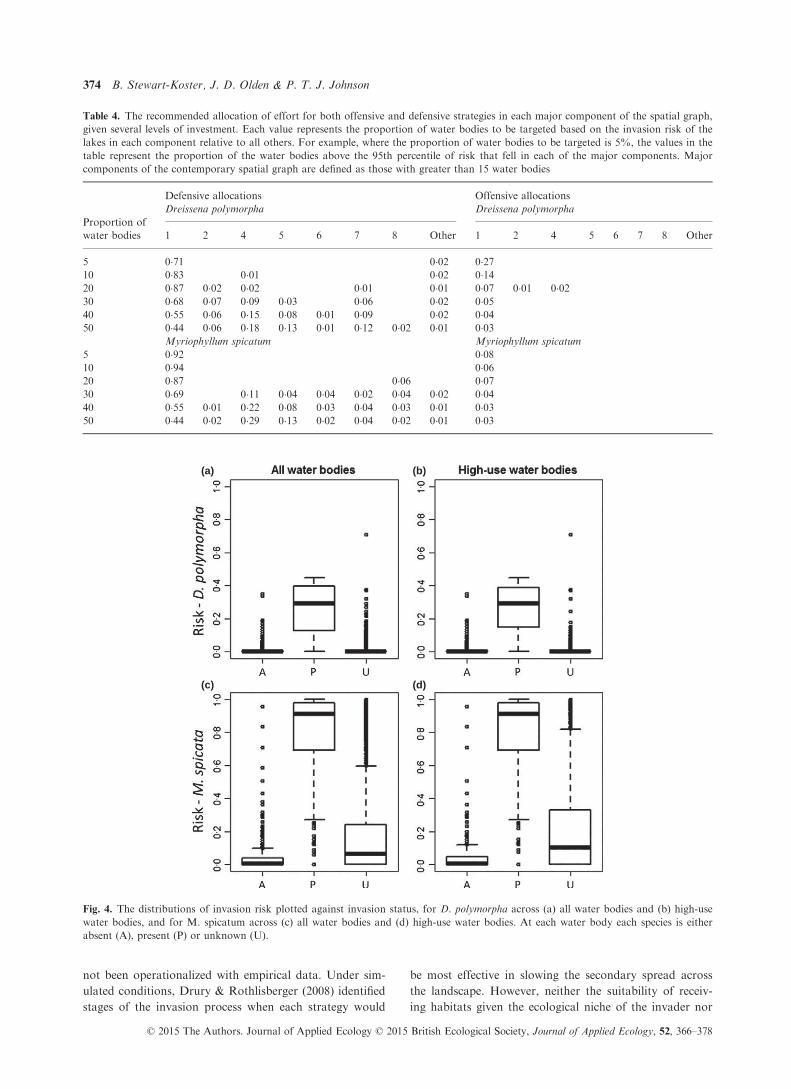
between water bodies observed to be invaded and unin-

vaded by D. polymorpha (Fig. 4a) and had an area under

the ROC curve of 0�97, which is slightly higher than the

spatial GAM. This pattern was consistent for high-use

water bodies (Fig. 4b). The spatial distribution of risk for

D. polymorpha was heavily skewed towards the south-

eastern part of the study region, which largely comprised

component 1 (Fig. 3c; Table 3). This is due to the gener-

ally higher habitat suitability and connectivity in that part

of the graph (Table 3). Subsequently, analyses for alloca-

tion of effort suggested component 1 should receive the

greatest allocation of effort for both offensive and defen-

sive strategies (Table 4). Should management budgets

allow for only 5% of water bodies to be protected, 71%

of this effort should be allocated to defensive strategies at

water bodies in component 1, with 27% allocated to

offensive strategies in component 1 and 2% allocated to

defensive strategies in other components. As management

budgets allow for a greater proportion of water bodies to

be targeted, our results suggest that other components

should receive allocation of effort for both offensive and

defensive strategies. It is not until it is possible to target

50% of all water bodies that all components should

receive some allocation of management effort for D. poly-

morpha.

The relatively high risk of invasion by M. spicatum was

distributed across most components of the spatial graph

with most of the high-risk water bodies contained in

components 1 and 8 (Table 3; Fig. 3d), a pattern consis-

tent with the predictions from the habitat suitability mod-

els. As with D. polymorpha, our risk metric was able to

discriminate well between water bodies observed to be

invaded and uninvaded by M. spicatum (Fig. 4c), with an

area under the ROC curve of 0�93, which is comparable

to the spatial GAM. The distributions of risk for M. spic-

atum were also similar for high-use water bodies (Fig. 4d).

Despite the more relatively even distribution of risk across

the region, the water bodies with the highest risk were

predominantly located in component 1. Consequently, it

is only under management plans that allow for more than

20% of the water bodies to be targeted for intervention

that another component, in this case component 8, should

receive management activities targeting M. spicatum

(Table 4).

Discussion

Increasing evidence of the ecological and economic

impacts of species invasions has emphasised the urgent

need for researchers to provide managers with meaningful

recommendations for how to both prevent invasions and

prioritize management of invasive species (Papes� et al.

2011). The notion of offensive and defensive strategies in

invasive species management provides a very useful frame-

work to guide preventive measures aimed at limiting the

secondary spread of non-native species, but until now has

Table 2. Parameter estimates for the generalised additive models of invasion vulnerability for the two invasive species. Only significant

variables, as determined by analysis of deviance, were used in the final models

Species Predictor variable Estimate (SE) Reduction in deviance P-value

Dreissena polymorpha Watershed area 0�87 (0�25) 12 <0�001Maximum depth 0�71 (0�27) 7�1 0�007Secchi depth 0�82 (0�31) 7�2 0�007Drainage lake 2�17 (0�61) 12�5 <0�001Distance to GL �1�19 (0�57) 4�4 0�04S(longitude, latitude) 41�8 <0�001

Myriophyllum spicatum Conductance 0�95 (0�47) 4 0�045Distance to GL �1�28 (0�75) 3 0�085S(longitude, latitude) 77�1 <0�001

Table 3. Summary statistics of the major components in the contemporary spatial graph for both species, including the number of water

bodies sampled (ni), the proportion known to be invaded (pi), predicted habitat suitability, and estimated invasion risk

Component

Dreissena polymorpha Myriophyllum spicatum

Observations Habitat suitability Invasion risk Observations Habitat suitability Invasion risk

ni pi Mean Max Mean Max ni pi Mean Max Mean Max

1 (n = 1 295) 163 0�42 0�14 0�99 0�04 0�71 326 0�97 0�84 1 0�75 1

2 (n = 164) 13 0�08 0�02 0�58 0 0�01 7 0�71 0�29 0�96 0�06 0�234 (n = 1 123) 28 0�07 0�007 0�77 0 0�02 64 0�41 0�34 0�99 0�13 0�75 (n = 791) 55 0 0�004 0�17 0 0 142 0�2 0�24 0�93 0�08 0�566 (n = 65) 1 0 0�003 0�02 0 0 3 0�33 0�61 0�93 0�38 0�627 (n = 411) 21 0 0�006 0�54 0 0 28 0�14 0�25 0�81 0�08 0�398 (n = 57) 9 0 0�004 0�03 0 0 7 1 0�92 0�99 0�86 0�96



92°W 90°W 88°W

42°N

44°N

46°N

Lake Superior

La

ke

Mi c

hi g

an

Illinois

Iowa

Minnesota

Michigan

92°W 90°W 88°W

42°N

44°N

46°N

Wisconsin

50 0 50 kilometers25

0.81 1.00

0.61 0.80

0.41 0.60

0.21 0.40

0.00 –

–

–

–

–

0.20

Lake Superior

La

ke

Mi c

hi g

an

Illinois

Iowa

Minnesota

Michigan

92°W 90°W 88°W

42°N

44°N

46°N

Wisconsin


0

0

0

5

0.41 1.0

0.21 0.4

0.06 0.2

0.01–

–

–

–

0.0

0.00

Lake Superior

La

ke

Mi c

hi g

an

Illinois

Iowa

Minnesota

Michigan

92°W 90°W 88°W

42°N

44°N

46°N

Wisconsin


0.81 1.00

0.61 0.80

0.41 0.60

0.21 0.40

0.00 –

–

–

–

–

0.20

(a) (b)

(c) (d)

Lake Superior

La

ke

Mi c

hi g

an

Illinois

Iowa

Minnesota

Michigan

Wisconsin


0.41 – 1.00

0.21 – 0.40

0.11 –0.20

0.01 – 0.10

0.00

D. polymorpha – habitat suitability M. spicatum – habitat suitability

D. polymorpha – invasion risk M. spicatum – invasion risk

Fig. 3. Predicted habitat suitability as predicted by the spatial GAMs, for (a) D. polymorpha and (b) M. spicatum, and estimated inva-

sion risk for (c) D. polymorpha and (d) M. spicatum integrating habitat suitability and probable connectivity of each water body. Symbol

size reflects habitat suitability or invasion risk.



not been operationalized with empirical data. Under sim-

ulated conditions, Drury & Rothlisberger (2008) identified

stages of the invasion process when each strategy would

be most effective in slowing the secondary spread across

the landscape. However, neither the suitability of receiv-

ing habitats given the ecological niche of the invader nor

Table 4. The recommended allocation of effort for both offensive and defensive strategies in each major component of the spatial graph,

given several levels of investment. Each value represents the proportion of water bodies to be targeted based on the invasion risk of the

lakes in each component relative to all others. For example, where the proportion of water bodies to be targeted is 5%, the values in the

table represent the proportion of the water bodies above the 95th percentile of risk that fell in each of the major components. Major

components of the contemporary spatial graph are defined as those with greater than 15 water bodies

Proportion of

water bodies

Defensive allocations Offensive allocations

Dreissena polymorpha Dreissena polymorpha

1 2 4 5 6 7 8 Other 1 2 4 5 6 7 8 Other

5 0�71 0�02 0�2710 0�83 0�01 0�02 0�1420 0�87 0�02 0�02 0�01 0�01 0�07 0�01 0�0230 0�68 0�07 0�09 0�03 0�06 0�02 0�0540 0�55 0�06 0�15 0�08 0�01 0�09 0�02 0�0450 0�44 0�06 0�18 0�13 0�01 0�12 0�02 0�01 0�03

Myriophyllum spicatum Myriophyllum spicatum

5 0�92 0�0810 0�94 0�0620 0�87 0�06 0�0730 0�69 0�11 0�04 0�04 0�02 0�04 0�02 0�0440 0�55 0�01 0�22 0�08 0�03 0�04 0�03 0�01 0�0350 0�44 0�02 0�29 0�13 0�02 0�04 0�02 0�01 0�03

(a) (b)

(c) (d)

Fig. 4. The distributions of invasion risk plotted against invasion status, for D. polymorpha across (a) all water bodies and (b) high-use

water bodies, and for M. spicatum across (c) all water bodies and (d) high-use water bodies. At each water body each species is either

absent (A), present (P) or unknown (U).



the connectivity among those habitats was considered.

Further, the constraint of large numbers of potential habi-

tats to protect with limited resources means that some

form of prioritisation is required. Here, we developed and

presented an approach that integrates the notion of offen-

sive and defensive strategies into recent frameworks repre-

senting integrative approaches to risk assessment (Vander

Zanden & Olden 2008; Leung et al. 2012; Ib�a~nez et al.

2014). Our goal was to demonstrate an integrated model-

ling approach that incorporated separate axes of the inva-

sion process (i.e. colonisation vs. establishment) and

provided guidelines for management intervention at

multiple scales. Because sufficient data to estimate popula-

tion demographic parameters are often lacking, we

sought an empirical approach that did not rely on

dynamic population models. Rather, we integrated

estimated habitat suitability and probable connectivity

based on empirical distribution of boater behaviour from

the region.

Using this approach for two different species, we identi-

fied an allocation of effort and a specific subset of water

bodies for offensive and defensive strategies. This infor-

mation can help ensure invasive species intervention mea-

sures are distributed most efficiently. Overall, the

estimates of risk were much higher for M. spicatum than

D. polymorpha, which reflects the generally higher pre-

dicted habitat suitability for M. spicatum. The improved

classification accuracy of our risk metric for D. polymor-

pha and its comparable accuracy for M. spicatum, when

compared to the spatial statistical models alone, provide

strong evidence of support for this estimate of risk. Our

approach provides flexibility for stakeholders to identify

priority sites for prevention efforts given a maximum level

of acceptable risk or based on budgetary/time restrictions

that may limit the number of locations that can be man-

aged. Placing additional priority on high-use water bodies,

reservoirs or those that are of high risk for both species

would assist in identifying the highest priority water

bodies for a given management plan. Finally, the water

body and component-level analysis provide a multiscale

perspective to identify broader regions (network compo-

nents) that may be suitable for larger scale interventions

such as component-wide boater education programmes or

wash down stations in population centres. Additionally,

the 60 component graph could be used to guide mesoscale

interventions, potentially administered at the local govern-

ment level (i.e. county or lake districts).

The arrival of invaders at uninvaded habitat is arguably

the most important step of the invasion process (Lock-

wood, Cassey & Blackburn 2005), making attempts to

quantify this process vital. We converted road distances

to probabilities based on the empirical distribution of

boater movements in the region reported by Buchan &

Padilla (1999). By using road distances in this way, we

could more faithfully represent the dispersal process asso-

ciated with species’ entrainment on recreational boats

than if we had used some other distance measure, such as

straight-line distance (Drake & Mandrak 2010). We were

required to assume that the county centroid represented

the average boater’s home to accommodate that the

majority of recreational boating trips are to a single water

body each day (Buchan & Padilla 1999). This assumption

will almost certainly overestimate the connectivity of some

water bodies and underestimate the connectivity of others.

However, in the absence of information about specific

trips or the physical addresses of registered boaters, this

assumption is unavoidable at this stage. It is nonetheless

a reasonable one since the overwhelming majority of fish-

ing trips are to a single water body and subsequent inva-

sive species introductions occur on later trips to others

(Peterson & Nelson 2008).

Improvements in the estimation of connectivity and its

validation could come from data pertaining to the nodes

(water bodies) or the links (the road network). Empirical

data derived from surveys of patterns of use at specific

water bodies or probabilistic estimates of attraction simi-

lar to gravity models could be used to weight nodes

according to their popularity. Equally, the distance

between pairs of lakes could be weighted by the quality of

the roads connecting them to derive connections based on

distance and ease of access. In addition to these improve-

ments, dispersal processes where the species move through

the network of water bodies unassisted, either through

drift or through active dispersal along drainage channels,

could be incorporated. We specifically looked at human-

assisted movements to target under the risk assessment

framework as this is generally the primary vector of

spread for many species (Vander Zanden & Olden 2008).

However, recent theoretical work predicting metapopula-

tion persistence of several species, based on within net-

work and overland dispersal of aquatic organisms,

demonstrated the likely importance of both processes to

metapopulation persistence, particularly for D. polymor-

pha (Mari et al. 2014). Our approach could be extended

by developing a spatial graph of the drainage network

and estimating connections according to empirical data

on instream species movements.

Graph and network theoretical approaches offer a

promising methodology to quantifying connectivity (or

potential connectivity) in complex networks (Dale &

Fortin 2010), especially freshwater ecosystems (Stewart-

Koster et al. 2007; Er}os et al. 2012; Rolls et al. 2014). A

network approach to modelling dispersal has already

demonstrated utility in understanding the spread of inva-

sive species (e.g. Muirhead & MacIsaak 2005; Drake &

Mandrak 2010). The development of numerous graph-the-

oretical indices that describe the connectivity of a given

system at a node and network level (e.g. Galpern,

Manseau & Fall 2011) may provide further opportunity

to advance invasive species research. Such indices can be

used to identify important hubs in a network given their

location and connectivity. The removal of such hubs from

the network of invasive species spread (i.e. offensive or

defensive protection) would reduce the connectivity of the



system most substantially, thereby decreasing the vulnera-

bility of the entire system (e.g. Florance et al. 2011). It

may not necessarily be the most highly connected node

that is most important, particularly for random as

opposed to scale-free networks (Barab�asi 2009). In the

present study, the difference between the historical and

contemporary spatial graphs highlighted the importance

of artificial reservoirs in reducing the average dispersal

distance required for the invasive species to access unin-

vaded locations. These types of habitats are known to

facilitate invasions into new locations (Johnson, Olden &

Vander Zanden 2008). Expected changes to the system

that improve accessibility such as such as the construction

of new boat launches or additional reservoirs could also

be incorporated into future spatial graphs of the system.

Beyond invasion hubs, graph-theoretical indices can be

applied to links in the network to identify the most

important potential invasion pathways, which if removed

(i.e. offensive protection at appropriate invaded water

bodies) would also reduce system-wide connectivity. These

could also be applied to road quality and accommodate

new road developments that improve access to uninvaded

water bodies.

Subsequent to the initial arrival of a species, the success-

ful establishment of a population is dependent on several

factors including the local habitat suitability. We quantified

this component of the invasion process using spatial GAMs

with environmental variables that may act as abiotic con-

straints on species establishment (Peterson & Vieglais

2001). These models, which accounted for approximately

half of the deviance in the spatial distribution for each spe-

cies, provided an avenue to predict invasion vulnerability at

unsampled water bodies given local environmental condi-

tions and any additional spatial processes not necessarily

accounted for by the spatial graph. Improving the deviance

explained and the predictive accuracy of the models would

improve our approach and could be achieved through the

use of additional predictor variables including biotic infor-

mation, as well as mechanistic modelling approaches such

as biophysical ecological models (Ib�a~nez et al. 2014). Addi-

tionally, modelling expected environmental and climate

changes could facilitate a predictive risk assessment that

accommodates how the invasion vulnerability of water

bodies in the system may change.

Dreissena polymorpha and M. spicatum had quite differ-

ent spatial distributions of predicted risk despite the dis-

persal of both being assisted via entrainment on both

boating and fishing equipment. This is no doubt a reflec-

tion of the different habitat requirements of each as well

as the difference in time since initial invasion, M. spica-

tum arrived 20–30 years before D. polymorpha (see Mate-

rials and Methods). Nonetheless, component 1 in the

contemporary spatial graph had the highest average inva-

sion risk for both species. This is not entirely unexpected

given its high number of reservoirs that are frequently

associated with species invasions in this region (Johnson,

Olden & Vander Zanden 2008) and its proximity to Lake

Michigan, which acts as a key source habitat. It is also

possible that both species are approaching a point of satu-

ration where invasion rates will start to decline because of

some process not included in the model. If this were the

case, the implicit assumption in the GAMs that the inva-

sion vulnerability of each water body is defined only its

location and the abiotic variables would result in the

degree and extent of invasion vulnerability being overesti-

mated. In such a scenario, the graph-theoretical analyses

still provide a useful first pass identifying vulnerability of

water bodies to new and still spreading invaders given

their potential connectivity (e.g. Johnson, Olden & Van-

der Zanden 2008; Olden, Vander Zanden & Johnson

2011). The economic and ecological impacts of these spe-

cies make such assessments critical.

In an age of limited public funds available for ecologi-

cal protection, it is imperative that the implementation of

invasive species management be targeted to locations of

the highest priority in all ecosystem types (Papes� et al.

2011). A risk assessment framework that combines as

many aspects of the invasion process as possible, such as

that presented here, provides an avenue to guide such

decisions. It is likely, given the already widespread spatial

distribution of M. spicatum, that some of the water bodies

with high and very high defensive priority are in fact

already invaded by this species. As such, it would be pru-

dent to conduct field sampling to determine the invasion

status to further refine the prioritisation. It is also impor-

tant to note that as with any risk assessment framework,

we are not advocating that the invasion vulnerability at

lower priority habitats be ignored. Rather, we are

attempting to aid decision-making as to where to apply

limited resources for management. Clearly, it would be

preferable to protect all uninvaded habitats and prevent

the invaders from leaving already invaded ones. However,

the reality of limited budgets and a growing number of

invasive species introductions mean that prioritisation is

crucial to slowing or even stopping their spread. The

approach presented here may assist with this process

across many ecosystem types.

Acknowledgements

We thank Dara Olson from the Great Lakes Indian Fish and Wildlife

Commission, Laura Herman, Susan Knight, Ron Martin from the Wis-

consin Department of Natural Resources, Pat Soranno, Kathy Webster

from the Michigan Department of Environmental Quality, David Balsiger

and from the North Temperate Lakes LTER program. We also thank

Jake Vander Zanden and Jeff Maxted from the University of Wisconsin

and Luke Rogers from the University of Washington for assistance with

road network connectivity. Finally, we thank two anonymous reviewers

whose comments substantially improved this manuscript. JDO was

supported by the H. Mason Keeler Endowed Professorship (School of

Aquatic and Fishery Sciences, University of Washington).

Data accessibility

Water body locations, environmental conditions and estimated invasion

risk, available at http://dx.doi.org/10.6084/m9.figshare.1285847 (Stewart-

Koster, Olden & Johnson 2015).



http://dx.doi.org/10.6084/m9.figshare.1285847

References

Arnott, S.E., Magnuson, J.J., Dodson, S.I. & Colby, A.C.C. (2006) Lakes

as islands: biodiversity, invasion, and extinction. Long Term Dynamics

of Lakes in the Landscape (eds J.J. Magnuson, T.K. Kratz & B.J. Ben-

son), pp. 67–88. Oxford Press, Oxford, UK.

Barab�asi, A.-L. (2009) Scale-free networks: a decade and beyond. Science,

325, 412–413.Benson, A. (2013) Zebra mussel sightings distribution. United States Geo-

logical Survey. http://nas.er.usgs.gov/

Berkman, P.A., Haltuch, M.A., Tichich, E., Garton, D.W., Kennedy,

G.W., Gannon, J.E., Mackey, S.D., Fuller, J.A. & Liebenthal, D.L.

(1998) Zebra mussels invade Lake Erie muds. Nature, 393, 27–28.Bivand, R.S., Pebesma, E.J. & G�omez-Rubio, V. (2008) Applied Spatial

Data Analysis with R. Springer-Verlag, New York, NY, USA.

Buchan, L.A.J. & Padilla, D.K. (1999) Estimating the probability of long-

distance overland dispersal of invading aquatic species. Ecological Appli-

cations, 9, 254–265.Carlton, J.T. (2008) The zebra mussel Dreissena polymorpha found in

North America in 1986 and 1987. Journal of Great Lakes Research, 34,

770–773.Connelly, N.A., O’Neill, C.R., Knuth, B.A. & Brown, T.L. (2007)

Economic impacts of zebra mussels on drinking water treatment and

electric power generation facilities. Environmental Management, 40, 105–112.

Dale, M.R.T. & Fortin, M.-J. (2010) From graphs to spatial graphs.

Annual Review of Ecology, Evolution and Systematics, 41, 21–38.Drake, D.A. & Mandrak, N.E. (2010) Least-cost transportation networks

predict spatial interaction of invasion vectors. Ecological Applications,

20, 2286–2299.Drury, K.L.S. & Rothlisberger, J.D. (2008) Offense and defense in land-

scape-level invasion control. Oikos, 117, 182–190.Epanchin-Niell, R.S., Hufford, M.B., Aslan, C.E., Sexton, J.P., Port, J.D.

& Waring, R.M. (2010) Controlling invasive species in complex social

landscapes. Frontiers in Ecology and the Environment, 8, 210–216.Er}os, T., Olden, J.D., Schick, R.S., Schmera, D. & Fortin, M.-J. (2012)

Characterizing connectivity relationships in freshwaters using patch-

based graphs. Landscape Ecology, 27, 303–317.Fausch, K.D., Rieman, B.E., Dunham, J.B., Young, M.K. & Peterson, D.P.

(2009) Invasion versus isolation: trade-offs in managing native salmonids

with barriers to upstream movement. Conservation Biology, 23, 859–870.Fielding, A.H. & Bell, J.F. (1997) A review of methods for the assessment

of prediction errors in conservation presence/absence models. Environ-

mental Conservation, 24, 38–49.Florance, D., Webb, J.K., Dempster, T., Kearney, M.R., Worthing, A. &

Letnic, M. (2011) Excluding access to invasion hubs can contain the

spread of an invasive vertebrate. Proceedings of the Royal Society B,

278, 2900–2908.Franklin, J. (2010) Moving beyond static species distribution models in

support of conservation biogeography. Diversity and Distributions, 16,

321–330.Gallien, L., M€unkem€uller, T., Albert, C.H., Boulangeat, I. & Thuiller, W.

(2010) Predicting potential distributions of invasive species: where to go

from here? Diversity and Distributions, 16, 331–342.Galpern, P., Manseau, M. & Fall, A. (2011) Patch-based graphs of land-

scape connectivity: a guide to construction, analysis and application for

conservation. Biological Conservation, 144, 44–55.Hastie, T.J. & Tibshirani, R.J. (1990) Generalized Additive Models. Chap-

man & Hall, London.

Hastings, A., Cuddington, K., Davies, K.F., Dugaw, C.J., Elmendorf, S.,

Freestone, A. et al. (2005) The spatial spread of invasions: new develop-

ments in theory and evidence. Ecology Letters, 8, 91–101.Higgins, S.N. & Vander Zanden, M.J. (2010) What a difference a species

makes: a meta–analysis of dreissenid mussel impacts on freshwater eco-

systems. Ecological Monographs, 80, 179–196.Hulme, P.E. (2009) Trade, transport and trouble: managing invasive spe-

cies pathways in an era of globalization. Journal of Applied Ecology, 46,

10–18.Hulme, P.E., Bacher, S., Kenis, M., Klotz, S., Kuhn, I., Minchin, D. et al.

(2008) Grasping at the routes of biological invasions: a framework for

integrating pathways into policy. Journal of Applied Ecology, 45, 403–414.

Ib�a~nez, I., Diez, J.M., Miller, L.P., Olden, J.D., Sorte, C.J.B., Blumenthal,

D.M. et al. (2014) Integrated assessment of biological invasions. Ecolog-

ical Applications, 24, 25–37.

Johnson, L.E. & Carlton, J.T. (1996) Post-establishment spread in large-

scale invasions: dispersal mechanisms of the zebra mussel Dreissena

polymorpha. Ecology, 77, 1686–1690.Johnson, P.T.J., Olden, J.D. & Vander Zanden, M.J. (2008) Dam invad-

ers: impoundments facilitate biological invasions into freshwaters. Fron-

tiers in Ecology and the Environment, 6, 357–363.Keddy, P.A. (1976) Lakes as islands: the distributional ecology of two

aquatic plants, Lemna minor L. and L. trisulca L. Ecology, 57, 163–359.Keith, D.A., Akc�akaya, H.R., Thuiller, W., Midgley, G.F., Pearson, R.G.,

Phillips, S.J., Regan, H.M., Ara�ujo, M.B. & Rebelo, T.G. (2008) Pre-

dicting extinction risks under climate change: coupling stochastic popu-

lation models with dynamic bioclimatic habitat models. Biology Letters,

4, 560–563.Leung, B. & Mandrak, N.E. (2007) The risk of establishment of aquatic

invasive species: joining invasibility and propagule pressure. Proceedings

of the Royal Society B, 274, 2603–2609.Leung, B., Roura-Pascual, N., Bacher, S., Heikkil€a, J., Brotons, L., Burg-

man, M.A. et al. (2012) TEASIng apart alien species risk assessments: a

framework for best practices. Ecology Letters, 15, 1475–1493.von der Lippe, M. & Kowarik, I. (2007) Long-distance dispersal of plants

by vehicles as a driver of plant invasions. Conservation Biology, 21, 986–996.

Lockwood, J.L., Cassey, P. & Blackburn, T. (2005) The role of propagule

pressure in explaining species invasions. Trends in Ecology and Evolu-

tion, 20, 223–228.Lodge, D.M., Williams, S., MacIsaac, H.J., Hayes, K.R., Leung, B., Rei-

chard, S. et al. (2006) Biological invasions: recommendations for U.S.

policy and management. Ecological Applications, 16, 2035–2054.Madsen, J.D. & Smith, D.H. (1997) Vegetative spread of Eurasian water-

milfoil colonies. Journal of Aquatic Plant Management, 35, 63–68.Mari, L., Casagrandi, R., Bertuzzo, E., Rinaldo, A. & Gatto, M. (2014)

Metapopulation persistence and species spread in river networks. Ecol-

ogy Letters, 17, 426–434.Moody, M.L. & Les, D.H. (2007) Geographic distribution and genotypic

composition of invasive hybrid watermilfoil (Myriophyllum spicatum 9

M. sibiricum) populations in North America. Biological Invasions, 9,

559–570.Muirhead, J.R. & MacIsaak, H.J. (2005) Development of inland lakes as

hubs in an invasion network. Journal of Applied Ecology, 42, 80–90.Nichols, S.A. & Martin, R. (1990) Wisconsin Lake Plant Database. Info.

Circ. 69, Wisconsin Geological and Natural History Survey, Madison.

Olden, J.D., Vander Zanden, M.J. & Johnson, P.T.J. (2011) Assessing eco-

system vulnerability to invasive rusty crayfish (Orconectes rusticus). Eco-

logical Applications, 21, 2587–2599.Papes�, M., Sallstrom, M., Asplund, T.R. & Vander Zanden, M.J. (2011)

Invasive species research to meet the needs of resource management and

planning. Conservation Biology, 25, 867–872.Pascual-Hortal, L. & Saura, S. (2006) Comparison and development of

new graph-based landscape connectivity indices: towards the prioriza-

tion of habitat patches and corridors for conservation. Landscape Ecol-

ogy, 21, 959–967.Peters, J.A. & Lodge, D.L. (2009) Invasive Species Policy at the Regional

Level: a Multiple Weak Links Problem. Fisheries, 34, 373–380.Peterson, K. & Nelson, E. (2008) Recreational Boating in Wisconsin: The

2007 Survey, Wisconsin Department of Natural Resources, pp 44.

Peterson, A.T. & Vieglais, D.A. (2001) Predicting species invasions using

ecological niche modeling: new approaches from bioinformatics attack a

pressing problem. BioScience, 51, 363–371.R Development Core Team (2012) R: A Language and Environment for

Statistical Computing. R Foundation for Statistical Computing, Vienna,

Austria. URL http://www.R-project.org/.

Rahel, F. (2013) Intentional fragmentation as a management strategy in

aquatic systems. BioScience, 63, 362–372.Robin, X., Turck, N., Hainard, A., Tiberti, N., Lisacek, F., Sanchez, J.-C.

& M€uller, M. (2011) pROC: an open-source package for R and S+ to

analyze and compare ROC curves. BMC Bioinformatics, 12, 77.

Rolls, R.J., Stewart-Koster, B., Ellison, T., Faggotter, S. & Roberts, D.T.

(2014) Multiple factors determine the effect of anthropogenic barriers to

connectivity on riverine fish. Biodiversity and Conservation, 23, 2201–2220.

Rothlisberger, J.D. & Lodge, D.M. (2009) Limitations of gravity models

in predicting the spread of Eurasian Watermilfoil. Conservation Biology,

25, 64–72.Rothlisberger, J.D., Chadderton, W.L., McNulty, J. & Lodge, D.M.

(2010) Aquatic invasive species transport via trailered boats: what is



http://nas.er.usgs.gov/

http://www.R-project.org/

being moved, who is moving it, and what can be done. Fisheries, 35,

121–132.Saura, S. & Torn�e, J. (2009) Conefor Sensinode 2.2: A software package

for quantifying the importance of habitat patches for landscape connec-

tivity. Environmental Modelling & Software, 24, 135–139.Smith, C.S. & Barko, J.W. (1990) Ecology of Eurasian watermilfoil. Jour-

nal of Aquatic Plant Management, 28, 55–64.Stewart-Koster, B., Kennard, M.J., Harch, B.D., Sheldon, F., Arthington,

A.H. & Pusey, B.J. (2007) Partitioning the variation in stream fish

assemblages within a spatio-temporal hierarchy. Marine and Freshwater

Research, 58, 675–686.Stewart-Koster, B., Olden, J.D. & Johnson, P.T.J. (2015) Data from: Inte-

grating landscape connectivity and habitat suitability to guide offensive

and defensive invasive species management. Figshare, http://dx.doi.org/

10.6084/m9.figshare.1285847.

Urban, D. & Keitt, T. (2001) Landscape connectivity: a graph-theoretic

perspective. Ecology, 82, 1205–1218.Vander Zanden, M.J. & Olden, J.D. (2008) A management framework for

preventing the secondary spread of aquatic invasive species. Canadian

Journal of Fisheries and Aquatic Sciences, 65, 1512–1522.Wilson, J.R.U., Dormontt, E.E., Prentis, P.J., Lowe, A.J. & Richardson,

D.M. (2009) Something in the way you move: dispersal pathways affect

invasion success. Trends in Ecology & Evolution, 24, 136–144.Wood, S.N. (2011) Fast stable restricted maximum likelihood and mar-

ginal likelihood estimation of semiparametric generalized linear models.

Journal of the Royal Statistical Society (B), 73, 3–36.

Received 29 September 2014; accepted 14 January 2015

Handling Editor: Shelley Arnott





integrating landscape connectivity and habitat suitability to guide

Documents