Integrated Inventory Routing and Freight Consolidation

for Perishable Goods

Weihong Hu Alejandro Toriello

H. Milton Stewart School of Industrial and Systems Engineering

Georgia Institute of Technology, Atlanta, GA

weihongh at gatech dot edu, atoriello at isye dot gatech dot edu

Maged Dessouky

Daniel J. Epstein Department of Industrial and Systems Engineering

University of Southern California, Los Angeles, CA

maged at usc dot edu

May 11, 2018

Abstract

We propose a model that integrates inventory routing and freight consolidation for perishable

goods with a fixed lifetime. The problem is motivated by the status quo of logistics in some

U.S. agriculture markets, but adapts to other relevant two-echelon supply chains, e.g. combined

production planning and distribution. We first identify special cases where solving single-echelon

subproblems sequentially yields an asymptotically optimal solution. For the general case, we

propose an iterative framework that consists of a decomposition procedure and a local search

scheme. In the decomposition, a freight consolidation subproblem is first solved to obtain crucial

shipping decisions, and after fixing these a restrictive model generates the other decisions for

the integrated problem. The local search aims at fast identification of good neighborhoods

by solving an assignment-style mixed-integer program that matches the consolidation decision

with an inventory routing subproblem, and gradually strengthens the incumbent solution pool

when executed in an iterative fashion. Experiments based on empirical demand distributions

demonstrate that our proposed iterative framework is quite efficient compared to a sequential

approach, and that it effectively solves challenging instances.

Keywords: logistics, inventory routing, freight consolidation

1 Introduction

Transportation is frequently the single largest element of total logistics cost, accounting for 50%-

65% [27]. A supplier often achieves efficient use of transportation assets by intelligently routing

1

a fleet to serve multiple customers. When transportation decisions are coupled with inventory

management, the resulting decisions are modeled by the inventory routing problem (IRP). Some

recent examples of successful IRP applications include Walmart’s vendor-managed inventory (VMI)

initiative [6] and ExxonMobil’s liquefied natural gas transportation and storage [36].

Nowadays, ever-increasing global competition encourages transportation cost savings through

horizontal cooperation within a supply chain echelon, such as when a warehouse consolidates differ-

ent suppliers’ orders to schedule outbound shipments at minimum total freight cost. One concrete

example is given by the plight of the California cut flower industry, where growers ship their prod-

uct individually to U.S. customers, and because of small disaggregated volumes, must usually incur

expensive less-than-truckload (LTL) or courier (e.g. FedEx, UPS) rates. In the last two decades,

this disadvantage has played a major role in California’s loss of over 40% of U.S. market share to

South American growers, who enjoy favorable full truckload (FTL) rates by aggregating products

prior to domestic distribution [35]. These authors estimate that California cut flower growers could

reduce annual transportation costs by $6 to $17 million via consolidation, depending on the number

of participating growers.

Vertical coordination across supply chain echelons is an additional avenue to reduce transporta-

tion costs. Although consolidation reduces outbound transportation costs with higher utilization

of shipping capacity, an excessive emphasis on it could restrict inbound shipping, and indirectly

lead to higher total costs. Moreover, it is hard to evaluate the impact of consolidation strategies

on inventory control at a facility without considering both echelons together. Therefore, many

agricultural sectors are realizing the collaboration imperative for growers, consolidation terminals,

sellers, and third-party carriers.

Cooperation and coordination offer benefits in almost every area, from procurement to last-mile

delivery. Besides the aforementioned truckload costs, economies of scale prevail when a vendor offers

batch ordering discounts, when a factory processes identical jobs on heterogeneous machines, when

a liner company ships different customers’ cargoes, etc. The ideal performance of the supply chain

could entail joint management of cross-functional activities such as production, transportation,

consolidation and inventory.

This paper integrates two classical problems that are typically solved independently in these

and similar supply chains. As interpreted in agriculture logistics, the first decision includes the

shipments and routes from local growers to a consolidation center, which is the short-haul problem

and can be modeled as an IRP; trucks are the only form of agriculture transportation in at least

80% of U.S. cities and communities [40], and thus the short-haul problem will generally involve a

routing component. The second decision concerns direct shipments from the consolidation center

to customers (retailers or wholesalers), the long-haul freight consolidation problem. The two sep-

arate models are already difficult and involve real-world complications like time-varying demand,

perishability, different truckload costs, routing capacities and duration limits. We propose the in-

tegrated problem, formulate it as a mixed-integer programming (MIP), and develop an iterative

2

framework with a decomposition procedure and a local search scheme to obtain solutions of high

quality in a reasonable amount of time. In the decomposition, a freight consolidation subproblem is

first solved to obtain long-haul FTL schedules, and after fixing these a restrictive model generates

the other decisions for the integrated MIP. The local search aims at fast identification of good

neighborhoods by solving an assignment-style MIP that matches the consolidation decision with

an IRP subproblem, and gradually strengthens the incumbent solution pool when executed in an

iterative fashion.

In the agricultural industry, long-haul transportation costs usually dominate the total distribu-

tion cost, which intuitively suggests a consolidation-based strategy. Hence, the “standard” approach

would be to first solve the long-haul freight consolidation problem, and use its shipping schedule

as the demand input for the short-haul IRP. However, our results show that overall costs can be

reduced by utilizing a system-wide optimization approach. We also demonstrate the potential of

the iterative framework in balancing solution efficacy and computational efficiency. The standard

approach tends to exceed 5 hours while solving a moderately-sized IRP subproblem, whereas our

proposed method yields near-optimal global solutions by exploring more neighborhoods in the same

amount of CPU time. When the planning horizon is longer, or there are more growers or sellers, our

approach can provide better solutions than CPLEX upper bounds as well as the standard approach,

and the advantage is enhanced as the problem size increases. On the other hand, we find that the

standard approach, or the seemingly counterintuitive “reverse” approach (which first optimizes the

IRP and uses its schedule as input for the consolidation subproblem), are asymptotically optimal

under some assumptions.

The remainder of the paper is organized as follows. We provide a brief literature review below

in §1.1. We formally state the problem in §2. We motivate and detail the iterative heuristic in §3.

We present experimental results in §4. We discuss potential future research and conclude in §5.

The appendix gives additional details not included in the body of the paper.

1.1 Literature Review

Both inventory routing and freight consolidation problems have drawn extensive attention in the

operations research community. The IRP simultaneously decides (1) when a central facility dis-

patches vehicles, (2) which customers a vehicle visits and in what order, and (3) how much demand

to fulfill or inventory to maintain at each facility. Over the past thirty years, numerous IRP models

have been studied with quite specific problem characteristics, among which the closest variants to

our short-haul problem are the class of finite horizon multi-period single-vehicle one-to-many IRP.

The solution techniques range from exact methods to meta-heuristics to optimization-based heuris-

tics. We refer the reader to [21] and [6] for comprehensive surveys on state-of-the-art methodologies

and industrial applications, respectively.

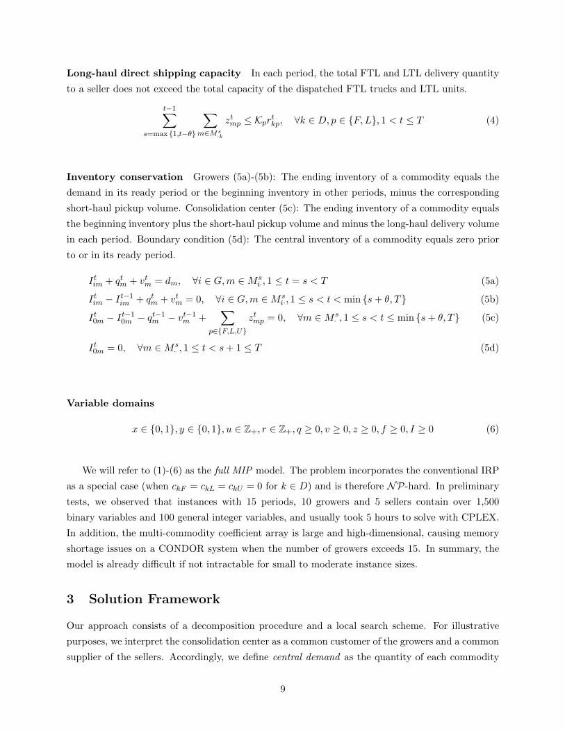
Freight consolidation addresses the question of how much volume or how many time periods to

accumulate before releasing a shipment that leverages economies of scale in transportation costs.

3

Since the pioneering work of [15, 28], quantity-based, time-based and hybrid policies have been

investigated; see [18] for a summary. In particular, [34, 35] proposed optimal and near-optimal

algorithms to solve the version of our long-haul problem without inventory aspects. When inventory

is taken into account, the long-haul decision can be viewed as a lot-sizing problem (LSP) where the

ordering cost function is piecewise linear (PWL), as depicted in Figure 1. Related research includes

the LSP with multiple set-up costs [5, 25, 33] and volume discounts [9, 19], but much of this work

usually assumes concave or monotonic properties that do not generalize to our case.

Figure 1: Volume-dependent long-haul shipping costs

The literature on the integration of inventory, routing, and consolidation is comparatively sparse.

Representative problems in this vein are the production routing problem (PRP) [4] and the maritime

inventory routing problem (MIRP) [36]. PRP coordinates two core supply chain functions, namely

production planning and distribution, which are the origins of LSP and IRP, and thus resemble

our long-haul and short-haul decisions, respectively. However, the few publications on this subject

concern much simpler settings, e.g. specified inventory replenishment rules [1, 16], uncapacitated

production and/or routing [37], fixed-charge or PWL concave production costs [3, 10, 12, 13, 14,

16, 17]. Furthermore, existing PRP models largely consider a homogeneous product from a single

plant to customers that do not restrict service time windows. In contrast, we treat the demand

for each grower-seller pair as an individual commodity, and impose hard constraints on the time in

transit or storage to accommodate the perishable nature of the agricultural product. On the other

hand, MIRP typically involves multiple commodities, loading/discharging time slots and intricate

cost elements, but fundamentally differs in network topology and does not share our cost structure.

Another related but less studied problem is the integration of various transportation modes in the

conventional IRP, e.g. when a main route serves a few major customers who then transship the

goods to minor customers via direct shipping [20].

From the perspective of solution approaches, many exact and heuristic IRP algorithms have

4

been successfully extended to MIRP and IRP with transshipment, whereas the PRP literature

centers more on heuristics. Early attempts are primarily meta-heuristics, especially those very

powerful in vehicle routing, e.g. GRASP [16], memetic algorithms [17], tabu search [10, 13]. Meta-

heuristics are capable of tackling PRP instances up to 200 customers and 20 time periods [16],

but the implementation is difficult because of the increased complexity in combined decisions and

constraints. Exact methods have also been developed, such as branch-and-price algorithms [14],

branch-and-cut algorithms [2, 8, 20, 37] and Lagrangian relaxations [26, 38], which unfortunately

are effective only for more basic variants and smaller problem instances. A seemingly promising

alternative is thus optimization-based heuristics. For example, [3] propose a hybrid adaptive large

neighborhood search (ALNS) scheme where upper-level search operators handle binary setup and

routing decisions, and lower-level network flow problems yield the corresponding production, inven-

tory and shipping quantities. Recently, [1] introduced a new two-phase scheme which considers a

lot-sizing problem with approximated routing costs first and a routing problem subsequently. Both

approaches exploit diversification mechanisms to prevent fast convergence to local optima in an

iterative fashion, and outperform previous methods for most benchmark instances with 14 to 200

customers and 6 to 20 time periods.

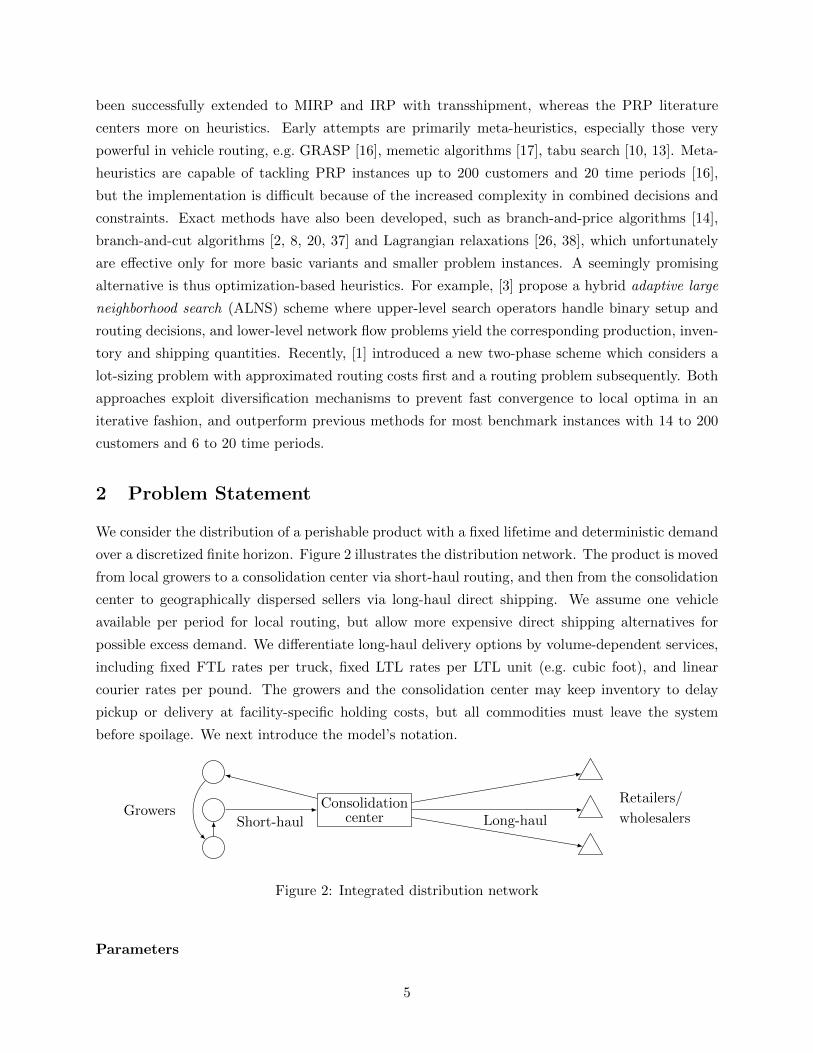
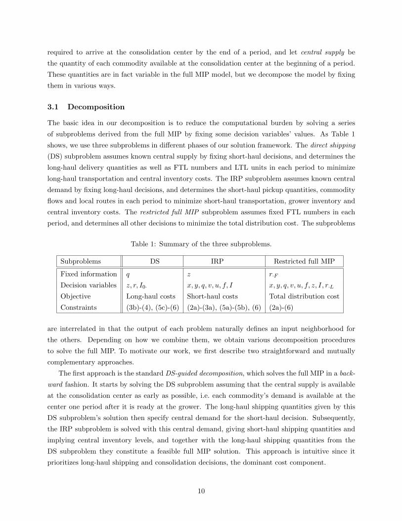
2 Problem Statement

We consider the distribution of a perishable product with a fixed lifetime and deterministic demand

over a discretized finite horizon. Figure 2 illustrates the distribution network. The product is moved

from local growers to a consolidation center via short-haul routing, and then from the consolidation

center to geographically dispersed sellers via long-haul direct shipping. We assume one vehicle

available per period for local routing, but allow more expensive direct shipping alternatives for

possible excess demand. We differentiate long-haul delivery options by volume-dependent services,

including fixed FTL rates per truck, fixed LTL rates per LTL unit (e.g. cubic foot), and linear

courier rates per pound. The growers and the consolidation center may keep inventory to delay

pickup or delivery at facility-specific holding costs, but all commodities must leave the system

before spoilage. We next introduce the model’s notation.

GrowersRetailers/

wholesalersConsolidation

centerShort-haul Long-haul

Figure 2: Integrated distribution network

Parameters

5

T : length of the planning horizon.

θ: product lifetime.

G, 0, D: set of growers, the consolidation center, and set of sellers, respectively.

m = M sik: a commodity tuple of product that is ready for pickup at the beginning of period

s and will be moved from grower i to seller k, ∀i ∈ G, k ∈ D, 1 ≤ s < T . M = {M sik} denotes

the set of all commodity tuples, and · indicates all elements with the respective indices. E.g.,

M ·i· is the set of commodities that originate from grower i.

dm: demand for commodity m.

Q: local vehicle capacity.

lij : local travel time from facility i to facility j, ∀i, j ∈ G∪{0}, i 6= j, scaled so that a route’s

maximum duration is one (i.e. one period in the planning horizon).

cij : local mileage cost from facility i to facility j, ∀i, j ∈ G ∪ {0}, i 6= j.

B: alternative short-haul direct shipping cost per shipment.

{F,L, U}: set of long-haul direct shipping modes, where F,L, U represent FTL, LTL and

courier services, respectively.

KF ,KL: maximum capacities in cubic feet for a FTL truck and a LTL unit, respectively.

ckF , ckL: transportation costs for an FTL truck and an LTL unit, respectively, from the

consolidation center to seller k, ∀k ∈ D.

α: conversion factor (lbs. per cubic foot).

ckU : transportation cost (per pound) for a courier shipment to seller k, ∀k ∈ D.

hi: inventory holding cost per unit product per period at facility i, ∀i ∈ G ∪ {0}.

The goal is to minimize the total transportation and inventory cost while satisfying all demands

before spoilage, and respecting local vehicle capacity, routing duration limits, as well as long-haul

shipping capacities for each FTL truck or LTL unit. We propose the MIP formulation below.

Decision variables

xtij =

1, arc (i, j) is traversed in period t

0, otherwise, ∀i, j ∈ G ∪ {0}, i 6= j, 1 ≤ t < T .

yt =

1, a local trip occurs in period t

0, otherwise, 1 ≤ t < T .

6

uti: number of alternative local vehicles used by grower i in period t, ∀i ∈ G, 1 ≤ t < T .

qtm: short-haul pick-up volume of commodity m in period t, ∀m ∈ M s. ,max {0, t− θ} < s ≤

t, 1 ≤ t < T .

vtm: volume of commodity m picked up in period t via alternative short-haul direct shipping,

∀m ∈M s. ,max {0, t− θ} < s ≤ t, 1 ≤ t < T .

f tijm: short-haul flow volume of commodity m on arc (i, j) in period t, ∀i, j ∈ G ∪ {0}, i 6=j,m ∈M s

. ,max {0, t− θ} < s ≤ t, 1 ≤ t < T .

ztmp: long-haul delivery volume of commodity m with mode p in period t, ∀p ∈ {F,L, U},m ∈M s. ,max {1, t− θ} ≤ s < t, 1 < t ≤ T .

rtkp: FTL numbers or LTL units sent to seller k in period t, ∀k ∈ D, p ∈ {F,L}, 1 < t ≤ T .

Itim: grower inventory of commoditym at the end of period t, ∀i ∈ G,m ∈M si.,max {0, t− θ} <

s ≤ t, 1 ≤ t < T .

It0m: central inventory of commodity m at the end of period t, ∀m ∈ M s. ,max {1, t− θ} ≤

s < t, 1 < t ≤ T .

Objective function The total distribution cost includes three parts: (1a) the short-haul trans-

portation cost, which equals regular arc routing costs plus alternative direct shipping costs; (1b) the

long-haul transportation cost, which is the sum of FTL trucks, LTL units and courier volume multi-

plied by their respective dispatch cost rates; (1c) the inventory cost, measured with facility-specific

holding cost rates.

minT−1∑t=1

∑i,j∈G∪{0},i 6=j

cijxtij +

T−1∑t=1

∑i∈G

Buti (1a)

+T∑t=2

∑k∈D

∑p∈{F,L}

ckprtkp + α

T∑t=2

t−1∑s=max {1,t−θ}

∑k∈D

∑m∈Ms

·k

ckUztmU (1b)

+

T−1∑t=1

∑i∈G

hi

t∑s=max {1,t−θ+1}

∑m∈Ms

i·

Itim + h0

T∑t=2

t−1∑s=max {1,t−θ}

∑m∈Ms

·

It0m (1c)

Route definition Arc degree constraints: Equalities (2a) and inequalities (2b) relate the node

degrees in the short-haul network to whether a trip occurs in each period. Specifically, the outdegree

of the consolidation center equals 1 if there is a trip, and 0 otherwise; the outdegree of a grower

is no more than that of the consolidation center. Constraints (2c) balance each facility’s indegree

and outdegree.

7

Commodity flow constraints (2d)-(2e): For a commodity originating at a specific grower, the

total outflow equals the total inflow plus the short-haul pickup volume in any period; for a com-

modity originating from other growers, the total outflow equals the total inflow. These constraints

also eliminate sub-tours.

Vehicle capacity constraints (2f)-(2g): The total volume carried by a regular vehicle does not

exceed its capacity on any arc traversed in each period; the total local direct shipping volume does

not exceed the total capacity of alternative vehicles dispatched from a grower in any period.

Duration constraints (2h): The total duration of a tour lasts no more than one period.∑i∈G

xt0i = yt, 1 ≤ t < T (2a)∑j∈G∪{0}

xtij ≤ yt, ∀i ∈ G, 1 ≤ t < T (2b)

∑j∈G∪{0},j 6=i

xtij −∑

j∈G∪{0},j 6=i

xtji = 0, ∀i ∈ G ∪ {0}, 1 ≤ t < T (2c)

∑j∈G∪{0},j 6=i

f tijm −∑

j∈G,j 6=if tjim = qtm, ∀i ∈ G,m ∈M s

i·,max {0, t− θ} < s ≤ t, 1 ≤ t < T (2d)

∑j∈G∪{0},j 6=i

f tijm −∑

j∈G,j 6=if tjim = 0, ∀i ∈ G,m /∈M s

i·,max {0, t− θ} < s ≤ t, 1 ≤ t < T (2e)

t∑s=max {1,t−θ+1}

∑m∈Ms

·

f tijm ≤ Qxtij , ∀i, j ∈ G ∪ {0}, i 6= j, 1 ≤ t < T (2f)

t∑s=max {1,t−θ+1}

∑m∈Ms·

i·

vtm ≤ Quti, ∀i ∈ G, 1 ≤ t < T (2g)

∑i,j∈G∪{0},i 6=j

lijxtij ≤ 1, 1 ≤ t < T (2h)

Demand satisfaction Short-haul (3a): For the short-haul echelon, the total pickup quantity

of each commodity, including regular routing and alternative direct shipping volume, equals its

demand. Long-haul (3b): For the long-haul echelon, the total delivery quantity of each commodity,

including FTL, LTL and courier volume, equals its demand.

min {s+θ,T}−1∑t=s

(qtm + vtm) = dm, ∀m ∈M s· , 1 ≤ s < T (3a)

min {s+θ,T}∑t=s+1

∑p∈{F,L,U}

ztmp = dm, ∀m ∈M s· , 1 ≤ s < T (3b)

8

Long-haul direct shipping capacity In each period, the total FTL and LTL delivery quantity

to a seller does not exceed the total capacity of the dispatched FTL trucks and LTL units.

t−1∑s=max {1,t−θ}

∑m∈Ms

·k

ztmp ≤ Kprtkp, ∀k ∈ D, p ∈ {F,L}, 1 < t ≤ T (4)

Inventory conservation Growers (5a)-(5b): The ending inventory of a commodity equals the

demand in its ready period or the beginning inventory in other periods, minus the corresponding

short-haul pickup volume. Consolidation center (5c): The ending inventory of a commodity equals

the beginning inventory plus the short-haul pickup volume and minus the long-haul delivery volume

in each period. Boundary condition (5d): The central inventory of a commodity equals zero prior

to or in its ready period.

Itim + qtm + vtm = dm, ∀i ∈ G,m ∈M si·, 1 ≤ t = s < T (5a)

Itim − It−1im + qtm + vtm = 0, ∀i ∈ G,m ∈M si·, 1 ≤ s < t < min {s+ θ, T} (5b)

It0m − It−10m − qt−1m − vt−1m +

∑p∈{F,L,U}

ztmp = 0, ∀m ∈M s· , 1 ≤ s < t ≤ min {s+ θ, T} (5c)

It0m = 0, ∀m ∈M s· , 1 ≤ t < s+ 1 ≤ T (5d)

Variable domains

x ∈ {0, 1}, y ∈ {0, 1}, u ∈ Z+, r ∈ Z+, q ≥ 0, v ≥ 0, z ≥ 0, f ≥ 0, I ≥ 0 (6)

We will refer to (1)-(6) as the full MIP model. The problem incorporates the conventional IRP

as a special case (when ckF = ckL = ckU = 0 for k ∈ D) and is therefore NP-hard. In preliminary

tests, we observed that instances with 15 periods, 10 growers and 5 sellers contain over 1,500

binary variables and 100 general integer variables, and usually took 5 hours to solve with CPLEX.

In addition, the multi-commodity coefficient array is large and high-dimensional, causing memory

shortage issues on a CONDOR system when the number of growers exceeds 15. In summary, the

model is already difficult if not intractable for small to moderate instance sizes.

3 Solution Framework

Our approach consists of a decomposition procedure and a local search scheme. For illustrative

purposes, we interpret the consolidation center as a common customer of the growers and a common

supplier of the sellers. Accordingly, we define central demand as the quantity of each commodity

9

required to arrive at the consolidation center by the end of a period, and let central supply be

the quantity of each commodity available at the consolidation center at the beginning of a period.

These quantities are in fact variable in the full MIP model, but we decompose the model by fixing

them in various ways.

3.1 Decomposition

The basic idea in our decomposition is to reduce the computational burden by solving a series

of subproblems derived from the full MIP by fixing some decision variables’ values. As Table 1

shows, we use three subproblems in different phases of our solution framework. The direct shipping

(DS) subproblem assumes known central supply by fixing short-haul decisions, and determines the

long-haul delivery quantities as well as FTL numbers and LTL units in each period to minimize

long-haul transportation and central inventory costs. The IRP subproblem assumes known central

demand by fixing long-haul decisions, and determines the short-haul pickup quantities, commodity

flows and local routes in each period to minimize short-haul transportation, grower inventory and

central inventory costs. The restricted full MIP subproblem assumes fixed FTL numbers in each

period, and determines all other decisions to minimize the total distribution cost. The subproblems

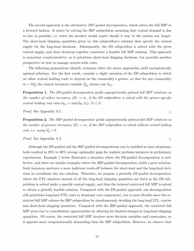
Table 1: Summary of the three subproblems.

Subproblems DS IRP Restricted full MIP

Fixed information q z r·F

Decision variables z, r, I0· x, y, q, v, u, f, I x, y, q, v, u, f, z, I, r·L

Objective Long-haul costs Short-haul costs Total distribution cost

Constraints (3b)-(4), (5c)-(6) (2a)-(3a), (5a)-(5b), (6) (2a)-(6)

are interrelated in that the output of each problem naturally defines an input neighborhood for

the others. Depending on how we combine them, we obtain various decomposition procedures

to solve the full MIP. To motivate our work, we first describe two straightforward and mutually

complementary approaches.

The first approach is the standard DS-guided decomposition, which solves the full MIP in a back-

ward fashion. It starts by solving the DS subproblem assuming that the central supply is available

at the consolidation center as early as possible, i.e. each commodity’s demand is available at the

center one period after it is ready at the grower. The long-haul shipping quantities given by this

DS subproblem’s solution then specify central demand for the short-haul decision. Subsequently,

the IRP subproblem is solved with this central demand, giving short-haul shipping quantities and

implying central inventory levels, and together with the long-haul shipping quantities from the

DS subproblem they constitute a feasible full MIP solution. This approach is intuitive since it

prioritizes long-haul shipping and consolidation decisions, the dominant cost component.

10

The second approach is the alternative IRP-guided decomposition, which solves the full MIP in

a forward fashion. It starts by solving the IRP subproblem assuming that central demand is due

as late as possible, i.e. when the product would expire should it stay in the system any longer.

The short-haul shipping quantities given by this subproblem’s solution then specify the central

supply for the long-haul decisions. Subsequently, the DS subproblem is solved with the given

central supply, and these decisions together constitute a feasible full MIP solution. This approach

is somewhat counterintuitive, as it prioritizes short-haul shipping decisions, but provides another

perspective on how to manage system-wide costs.

The following propositions identify scenarios when the above approaches yield asymptotically

optimal solutions. For the first result, consider a slight variation of the DS subproblem in which

we allow central holding costs to depend on the commodity’s grower, so that for any commodity

m = M sik the central inventory variable It0m incurs cost h0,i.

Proposition 1. The DS-guided decomposition yields asymptotically optimal full MIP solutions as

the number of sellers increases, |D| → ∞, if the DS subproblem is solved with the grower-specific

central holding cost rates h0,i = min{h0, hi}, ∀i ∈ G.

Proof. See Appendix A.1. �

Proposition 2. The IRP-guided decomposition yields asymptotically optimal full MIP solutions as

the number of growers increases, |G| → ∞, if the IRP subproblem is solved without central holding

cost, i.e. using h′0 = 0.

Proof. See Appendix A.2. �

Although the DS-guided and the IRP-guided decompositions can be justified in some situations,

both resulted in 20% to 30% average optimality gaps for realistic problem instances in preliminary

experiments. Example 1 below illustrates a situation where the DS-guided decomposition is inef-

fective, and there are similar examples where the IRP-guided decomposition yields a poor solution.

Such instances motivate a more judicious trade-off between the short-haul and the long-haul deci-

sions to coordinate the two echelons. Therefore, we propose a partially DS-guided decomposition,

where the FTL numbers instead of all the long-haul shipping quantities are fixed as the DS sub-

problem is solved under a specific central supply, and then the induced restricted full MIP is solved

to obtain a globally feasible solution. Compared with the DS-guided approach, our decomposition

still prioritizes long-haul FTL costs (a dominant cost component), but is more flexible since the re-

stricted full MIP relaxes the IRP subproblem by simultaneously deciding the long-haul LTL, courier

and short-haul shipping quantities. Compared with the IRP-guided approach, the restricted full

MIP gives rise to consolidation opportunities by allowing for limited changes in long-haul shipping

quantities. Of course, the restricted full MIP involves more decision variables and constraints, so

it appears more computationally demanding than the IRP subproblem. However, we observe that

11

the overall problem difficulty mainly stems from the routing decisions, and our approach achieves

a reasonable balance between solution quality and computational runtime.

Example 1. Consider a network with two growers and one retailer, where the planning horizon

length is T = 3 days, the product lifetime is θ = 2 days, and the local vehicles as well as the

long-haul FTL trucks have identical capacities, i.e. Q = KF . Suppose the holding cost rates are

such that h1 = h2 > h0 > 0. Let two orders be ready at the beginning of the planning horizon,

0.5Q for one grower and 0.5Q + ε (ε > 0) for the other. The total shipping volume exceeds the

FTL capacity by a small volume of ε units, which will be shipped via LTL or courier services in

the long-haul echelon. Since h0 > 0 and the long-haul transportation cost depends on the volume

rather than the shipping period, the optimal DS solution ships all KF + ε units on the second day

to minimize central inventory costs. In the consequent IRP subproblem, this results in a violation

of the local vehicle capacity on the first day and thus induces a penalty cost of B. On the other

hand, the global optimum would postpone ε units to the third day as a compromise between the

two echelons. The partially DS-guided decomposition attains this optimum since the final LTL and

courier schedules are subject to the simultaneous short-haul decisions. The excess total cost of the

DS-guided decomposition is then B − h2ε, which can be very high if the grower holding cost rate

is small.

The DS subproblem can be solved with CPLEX for moderate instances; the algorithms in

[34, 35] can handle large instances (e.g. T = 300) assuming just-in-time central supply (hi =

0, ci,j = 0,∀i, j ∈ G and so I ·0· = 0, which yields the lowest possible long-haul transportation cost).

The IRP subproblem and the restricted full MIP subproblem can be solved with CPLEX for small

instances; existing heuristics for IRP variants with time windows may also be employed to obtain

fast solutions for larger instances.

3.2 Local Search

Our motivation for developing a local search scheme is to escape poor local optima encountered in a

single iteration of the partially DS-guided decomposition. Despite the additional flexibility gained

over the DS-guided approach by substituting the IRP subproblem with the restricted full MIP,

there is no improvement guarantee on the resulting solution, even if the subproblems are solved to

optimality, which is unrealistic as the instance size increases. We next propose an optimization-

based local search scheme that takes advantage of the inherent incompatibility between the DS and

the IRP subproblems. We introduce some terminology before elaboration.

Definition 1 (Mismatched demand, MMD). Assume both IRP and DS subproblems are solved

simultaneously under given central demand and central supply assignments, respectively. A portion

of the demand for a commodity (i, k, s) is said to be mismatched if the short-haul pickup time ι and

the long-haul delivery time τ are incompatible, s < τ ≤ ι < min{s+ θ, T}; that is, the short-haul

12

solution collects this demand from the grower too late for its corresponding long-haul shipment.

We denote this mismatched subcommodity by (i, k, s, ι, τ).

Definition 2 (Service time windows). For a commodity (i, k, s), we may restrict the time in which

it can be picked up at the grower to the time interval [ι, ι], which we call its pickup time window,

where s ≤ ι ≤ ι < min{s+ θ, T}. Similarly, we may restrict the time in which the commodity can

be shipped from the center to the time interval [τ , τ ], which we call a delivery time window, where

s < τ ≤ τ ≤ min{s+ θ, T}.

From the perspective of transportation costs, later central demand benefits short-haul routing

whereas earlier central supply facilitates long-haul consolidation. Hence MMD can arise when the

IRP subproblem and the DS subproblem are solved separately under the respective central demand

and supply assumptions. In particular, the IRP solution with pickup windows [s,min{s + θ, T})and the DS solution with delivery windows (s,min{s + θ, T}] tend to be globally infeasible if

we piece them together into a full MIP solution. Narrowing service time windows corresponding

to MMD can eliminate this global infeasibility; for example, if (i, k, s, ι, τ) is a mismatched sub-

commodity with τ ≤ ι, we can revise the pickup window to be [s, τ) or the delivery window to be

(ι,min{s+ θ, T}], and the MMD will vanish when the subproblems are solved under the adjusted

service time windows. To hopefully balance the objectives of both subproblems, we may use a

pickup window [s, ζ) and a delivery window [ζ,min{s+θ, T}] where ι < ζ ≤ τ , or adjust the pickup

windows for a portion of the MMD and the delivery windows for the remaining units. The following

example illustrates the basic idea.

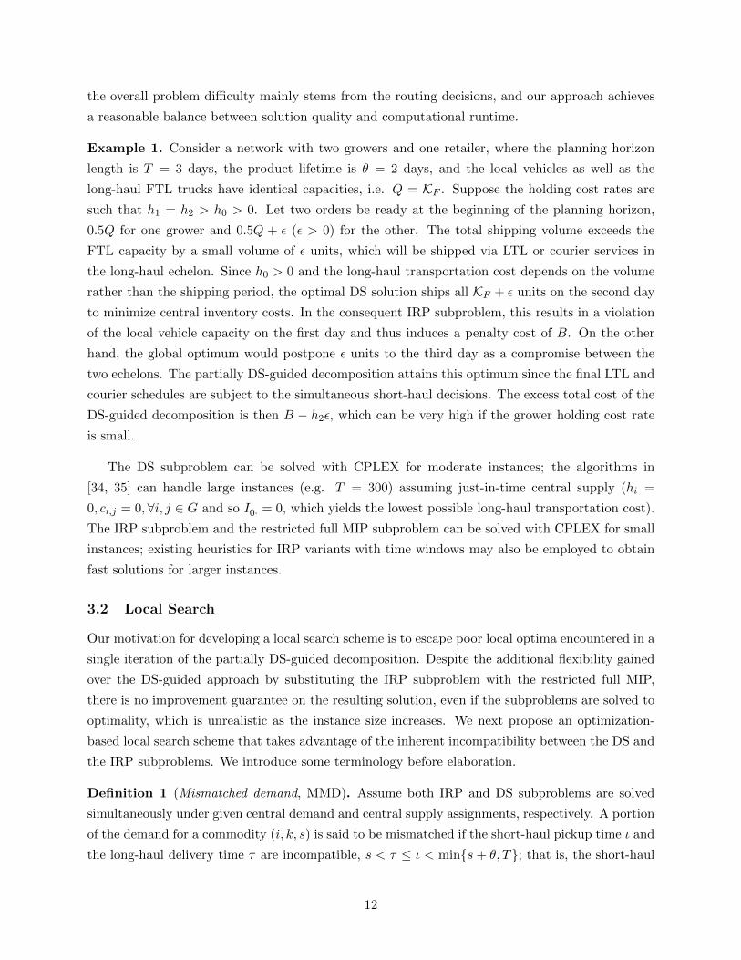
Example 2. Consider the time-space network in Figure 3. There are three planning periods, two

growers and two retailers, i.e. T = 3 days, G = {i, j}, D = {k, `}. The product has a lifetime θ = 2

days, and the demands are d1ik = 5, d1i` = 5, d2i` = 5, d1jk = 10, d2j` = 5. Suppose local mileage

costs are symmetric, holding costs are such that hi > h0 > hj , 0 < h0 < min{ckL, c`L}, and vehicle

capacities satisfy Q = KF = 15. For illustration purposes, the consolidation center is split into two

copies, representing the common IRP customer and the common DS supplier, respectively. Assume

the central supply is ready for long-haul delivery the day after a demand is ready for pickup at

the grower, whereas the central demand is not due until the expiration time or end of the horizon.

This encourages both single-echelon subproblems to best utilize transportation capacity.

Suppose we solve the subproblems with the given holding cost rates: The total demand is∑2s=1(d

sik+dsi`+d

sjk+dsj`) = 30 = 2Q, and the portion ready on the first day is d1ik+d1i`+d

1jk+d1j` =

20 = Q + 5. To avoid expensive direct shipping alternatives, the IRP subproblem tries to fully

utilize the local routing vehicle capacity, which means a volume of 5 units will be held in inventory

on day 1. Since hi > h0 > hj , grower i’s demands are prioritized whereas half of the demand for

commodity (j, k, 1) is delayed until day 2 for local pickup. On the other hand, the total demands for

retailer k and retailer ` both equal KF , and are expected to be ready for long-haul delivery on day 2

and day 3, respectively; hence the optimal DS subproblem solution sends out an FTL on each day.

13

This solution is outlined in Figure 3(a), where the bold numbers represent the quantities associated

with grower j and the others for grower i. The central flow imbalance from day 2 to day 3 indicates

that subcommodity (j, k, 1, 2, 2) induces an MMD of 5 units. Therefore, the corresponding full MIP

solution would be infeasible if we piece the subproblem solutions together. To remove the MMD,

we may keep the IRP solution and narrow the delivery window for commodity (j, k, 1) to day 3 in

the DS subproblem, or keep the DS solution and narrow the pickup window to day 1 in the IRP

subproblem. As a compromise, we may also take the approach illustrated by Figure 3(b), where

the pickup window for 2 units of the mismatched subcommodity (j, k, 1, 2, 2) is narrowed to day 1,

and the delivery window for the remaining 3 units is narrowed to day 3, respectively.

MMD essentially provides a guide to attain more compatible central demand and supply as-

signments for the subproblems. Since the modification of service time windows impacts routing,

consolidation and inventory decisions, we propose using a demand reasignment problem to deter-

mine the time window modifications. The input of this problem includes both relevant full MIP

parameters and extra data from the IRP and DS subproblem solutions. Specifically, we calculate

mismatched subproblem demands, residual short-haul and long-haul transportation capacities as

well as the remaining time allowed for each local route. We also estimate the routing cost and

duration changes for each pair of grower and route. If grower i is visited by a regular short-haul

vehicle in period t (route t), we approximate the routing cost savings of removing i from the route

with the amount obtained by joining i’s predecessor and successor when it is removed from route t.

Meanwhile, if grower i is not visited by route t, we approximate its insertion cost with the cheapest

insertion cost of inserting i into the route. We use the same approximations to estimate duration

changes.

Additional input

m = Msιτik : a mismatched subcommodity tuple, where a portion of demand dm is picked

up in period ι for the IRP subproblem and delivered in period τ for the DS subproblem,

m ∈ {M sik}, i ∈ G, k ∈ D, s < τ ≤ ι < min{s + θ, T}. Define M with the possible usage of ·

analogously to M in §2.

dm: demand for subcommodity m.

σti : indicator, equals 1 if grower i is visited by route t, 0 otherwise.

ηti+: insertion cost for grower-route pair (i, t), equals 0 if σti = 1.

lti+: duration increase for route t after inserting grower i, equals 0 if σti = 1.

ηti−: cost savings from removing i from t, equals 0 if σti = 0.

lti−: duration reduction for route t after removing grower i, equals 0 if σti = 0.

14

Day 1

i5+10

j

5

5

Day 2

i10+5

j

10

k10+5

`5+10

Day 3

k

`5+10

10+5 5

(a) Full MIP infeasibility due to MMD

Day 1

i7+8

j

7

2

3

Day 2

i8+7

j

8

k7+5

`

Day 3

k3

`5+10

7+8

8+7 3

(b) A reassignment strategy by narrowing pickup and delivery windows

Grower Consolidation center Retailer

Transportation arc Inventory arc

Figure 3: MMD and reassignment strategies

15

Lt: remaining time allowed for route t, equals 1 minus the duration of route t if it occurs, 1

otherwise.

Qt: residual capacity for route t, equals Q minus the total short-haul pickup volume for route

t if it occurs, Q otherwise.

Vtk: total FTL and LTL volume sent to seller k in period t in the DS subproblem solution.

Υtkp: number of FTL trucks or LTL units sent to seller k in period t in the DS subproblem

solution, p ∈ {F,L}.

The decision variables of the demand reassignment problem include insertion or removal for each

grower-route pair (i, t), short-haul pickup and long-haul delivery quantities for each mismatched

subcommodity, extra or saved FTL and LTL numbers, as well as courier volume and inventory

level changes in each period.

Decision variables

πti =

1, if grower i is inserted into route t

0, otherwise, i ∈ G, 1 ≤ t < T .

ρti =

1, if grower i is removed from route t

0, otherwise, i ∈ G, 1 ≤ t < T .

νt =

1, if the new route t exceeds capacity or duration limit

0, otherwise, 1 ≤ t < T .

ωtm ∈ R+: reassigned short-haul pickup volume of subcommodity m to route t, m ∈Ms·· , 1 ≤

s ≤ t < min{s+ θ, T}.

δtm ∈ R+: reassigned long-haul delivery volume of subcommodity m in period t, m ∈ Ms·· ,

1 ≤ s < t ≤ min{s+ θ, T}.

rtkp+, rtkp− ∈ Z+: extra and saved FTL or LTL numbers, respectively, dispatched to seller k

in period t, k ∈ D, p ∈ {F,L}, 1 < t ≤ T .

ztk+, ztk− ∈ R+: extra and saved courier volume, respectively, shipped to seller k in period t,

k ∈ D, 1 < t ≤ T .

Itim+, Itim− ∈ R+: inventory increase and reduction, respectively, of subcommodity m at

grower i in period t, m ∈Ms·i· , i ∈ G, 1 ≤ s ≤ t < min{s+ θ, T}.

It0m ∈ R+: central inventory of subcommodity m in period t, m ∈ Ms·· , 1 ≤ s < t ≤

min{s+ θ, T}.

16

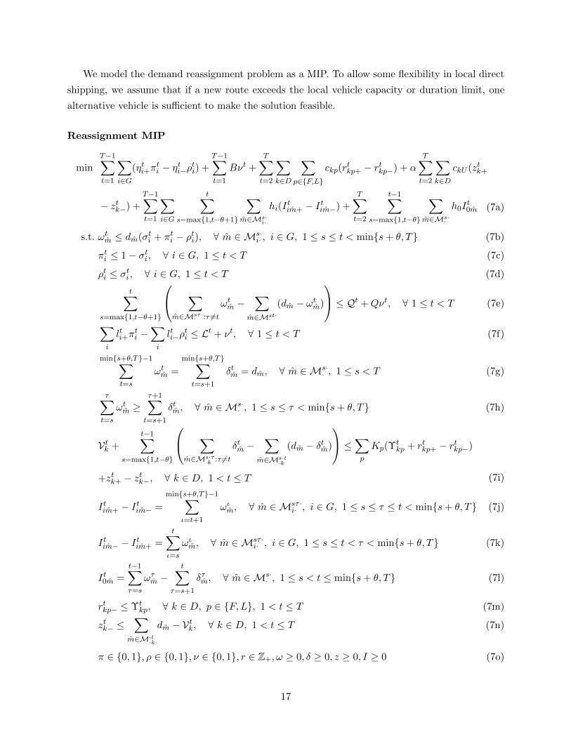
We model the demand reassignment problem as a MIP. To allow some flexibility in local direct

shipping, we assume that if a new route exceeds the local vehicle capacity or duration limit, one

alternative vehicle is sufficient to make the solution feasible.

Reassignment MIP

minT−1∑t=1

∑i∈G

(ηti+πti − ηti−ρti) +

T−1∑t=1

Bνt +T∑t=2

∑k∈D

∑p∈{F,L}

ckp(rtkp+ − rtkp−) + α

T∑t=2

∑k∈D

ckU (ztk+

− ztk−) +T−1∑t=1

∑i∈G

t∑s=max{1,t−θ+1}

∑m∈Ms·

i·

hi(Itim+ − Itim−) +

T∑t=2

t−1∑s=max{1,t−θ}

∑m∈Ms·

·

h0It0m (7a)

s.t. ωtm ≤ dm(σti + πti − ρti), ∀ m ∈Ms·i· , i ∈ G, 1 ≤ s ≤ t < min{s+ θ, T} (7b)

πti ≤ 1− σti , ∀ i ∈ G, 1 ≤ t < T (7c)

ρti ≤ σti , ∀ i ∈ G, 1 ≤ t < T (7d)

t∑s=max{1,t−θ+1}

∑m∈Msτ ·

· :τ 6=tωtm −

∑m∈Mst·

·

(dm − ωtm)

≤ Qt +Qνt, ∀ 1 ≤ t < T (7e)

∑i

lti+πti −

∑i

lti−ρti ≤ Lt + νt, ∀ 1 ≤ t < T (7f)

min{s+θ,T}−1∑t=s

ωtm =

min{s+θ,T}∑t=s+1

δtm = dm, ∀ m ∈Ms·· , 1 ≤ s < T (7g)

τ∑t=s

ωtm ≥τ+1∑t=s+1

δtm, ∀ m ∈Ms·· , 1 ≤ s ≤ τ < min{s+ θ, T} (7h)

Vtk +

t−1∑s=max{1,t−θ}

∑m∈Ms·τ

·k :τ 6=tδtm −

∑m∈Ms·t

·k

(dm − δtm)

≤∑p

Kp(Υtkp + rtkp+ − rtkp−)

+ztk+ − ztk−, ∀ k ∈ D, 1 < t ≤ T (7i)

Itim+ − Itim− =

min{s+θ,T}−1∑ι=t+1

ωιm, ∀ m ∈Msτ ·i· , i ∈ G, 1 ≤ s ≤ τ ≤ t < min{s+ θ, T} (7j)

Itim− − Itim+ =t∑ι=s

ωιm, ∀ m ∈Msτ ·i· , i ∈ G, 1 ≤ s ≤ t < τ < min{s+ θ, T} (7k)

It0m =t−1∑τ=s

ωτm −t∑

τ=s+1

δτm, ∀ m ∈Ms·· , 1 ≤ s < t ≤ min{s+ θ, T} (7l)

rtkp− ≤ Υtkp, ∀ k ∈ D, p ∈ {F,L}, 1 < t ≤ T (7m)

ztk− ≤∑

m∈M·t·k

dm − Vtk, ∀ k ∈ D, 1 < t ≤ T (7n)

π ∈ {0, 1}, ρ ∈ {0, 1}, ν ∈ {0, 1}, r ∈ Z+, ω ≥ 0, δ ≥ 0, z ≥ 0, I ≥ 0 (7o)

17

The objective (7a) is to minimize the total net rerouting and reconsolidation cost. Note that

we calculate net inventory cost changes at the growers, but only consider inventory costs after

reassignment at the consolidation center. (7b)-(7d) ensure that the binary rerouting variables are

correctly updated to form a new route, i.e. pickup can occur only if a grower is visited; insertion

can occur only if the grower was not visited in the original IRP subproblem solution; removal

can occur only if the grower was visited. (7e)-(7f) are short-haul transportation capacity and

duration constraints, i.e. the net increase of reassigned pickup volume does not exceed the residual

regular vehicle capacity plus alternative capacity in each period; similarly, the net increase of

duration after reassignment does not exceed the residual time of the original regular route plus

the length of a possible alternative direct shipping trip (i.e. one period). (7g)-(7h) are demand

satisfaction constraints redefined for each MMD, i.e. the total short-haul pickup volume equals

the total long-haul delivery volume after reassignment; at any point before the product spoils, the

total short-haul pickup volume to date is no less than the total long-haul delivery volume by the

next period. (7i) are aggregated direct shipping capacity constraints after canceling out the courier

volume, i.e. the net increase of reassigned delivery volume to a seller does not exceed the residual

long-haul transportation capacity plus the extra capacity in each period. (7j)-(7l) are inventory

balance constraints, i.e. the grower’s inventory of any MMD in period t increases by the total later

reassigned short-haul pickup volume if it was shipped by period t in the original IRP solution;

the grower’s inventory of any MMD in period t decreases by the total short-haul pickup volume

reassigned earlier than or in period t if it was shipped after that in the original IRP solution;

the central inventory of any MMD in period t equals the total short-haul pickup volume that has

arrived minus the total long-haul volume that has been delivered to the seller. (7m)-(7n) and (7o)

are boundary conditions and the domain, respectively.

At first glance, the reassignment MIP (7) may appear complicated and similar in structure to

the full MIP. However, it exhibits several features that enable efficient optimization: First, decisions

for matched demands are fixed so the problem size is smaller than the full MIP; second, combina-

torial rerouting costs are approximated linearly; third, complex subtour elimination constraints are

circumvented with the introduction of simple binary variables. In our experiments, CPLEX solved

it almost instantly in most cases.

3.3 An Iterative Framework

We have set up an optimization problem for local search in hope of eliminating MMD at the lowest

cost. We note the following issues:

• We fix the subproblem decisions for matched demands before solving Model (7). If a grower is

removed from a tour but only a fraction of the shipment was mismatched, then the matched

portion should also be removed from the tour and the residual vehicle capacity should be

larger. Model (7) does not capture this.

18

• The approximate rerouting costs for the reassignment problem may differ from the optimal

values. For instance, the effect of rerouting multiple growers in a period is the corresponding

TSP tour cost change, which generally is not the summation of cost changes incurred by

each single grower. Similarly, the savings approximation of removing a single grower may

underestimate the true amount.

• The input quantities that Model (7) inherits from the subproblem solutions may not reflect

the full MIP solution induced by the reassigned quantities. For instance, the subproblems

start with predefined central demand and supply assignments, but the short-haul pickup or

long-haul delivery times are not revealed until the reassigned solution is determined; hence

the modeled central inventory levels may differ from the final outcome.

For these reasons, we do not count on finding high-quality full MIP solutions by solving Model

(7) once. Instead, we propose to obtain solutions by embedding the decomposition and the local

search in an iterative framework (Figure 4). Throughout the procedure, we record the best full

MIP solution found so far, and keep a count that determines when to terminate. We partition the

given commodities M into two subsets, where S contains the matched sub-commodities and Mthe mismatched subset. Both subsets will be updated from iteration to iteration. To initiate the

procedure, we set S = M, M = ∅, i.e. we assume all given demands are matched.

We begin with the most flexible transportation for both echelons, which is realized by fixing

the pickup windows to [s,min{s + θ, T}) and the delivery windows to (s,min{s + θ, T}] for each

m ∈M s· . This gives the latest possible central demand and the earliest possible central supply. We

first solve the DS subproblem and obtain the long-haul shipping quantities. Subsequently, we fix the

FTL numbers and solve the corresponding restricted full MIP. If a predefined maximum allowable

number of iterations N is not yet reached, we then solve the IRP subproblem and calculate all

mismatched demands in comparison to the DS solution. If there is any MMD, i.e. M 6= ∅ or∑m∈M dm > 0, we update the subset S = M \M, and go to the next iteration. Each new iteration

starts by solving Model (7), after which we adjust the mismatched sub-commodity service time

windows based on the reassigned quantities. For example, if the demand for Msιτik where τ ≤ ι

is reassigned to period ι′ for short-haul shipping and period τ ′ for long-haul shipping (ι′ < τ ′),

then we modify the pickup and delivery windows to be [s, τ ′) and (ι′,min{s+ θ, T}], respectively.

For the matched sub-commodities S, we use the initial service time windows to encourage higher

utilization of transportation capacities. Mathematically, this is equivalent to adding constraints∑τ ′

t=s qtm ≥

∑τ ′−1t=s ωtm in the IRP model and

∑min{s+θ,T}t=ι+1

∑p∈{F,L,U} z

tmp ≥

∑min{t+θ,T}t=ι+1 δtm in the

DS model for all m ∈M, where ω and δ are the shipping quantities reassigned by Model (7). The

adjusted service time windows induce new central demand and supply, and the iterative process

repeats itself until the maximum number of iterations is met or MMD no longer exists, where we

output the best full MIP solution and exit.

19

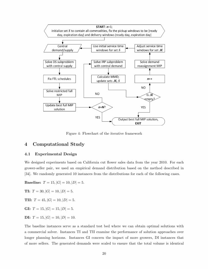
Figure 4: Flowchart of the iterative framework

4 Computational Study

4.1 Experimental Design

We designed experiments based on California cut flower sales data from the year 2010. For each

grower-seller pair, we used an empirical demand distribution based on the method described in

[34]. We randomly generated 10 instances from the distributions for each of the following cases.

Baseline: T = 15, |G| = 10, |D| = 5.

TI: T = 30, |G| = 10, |D| = 5.

TII: T = 45, |G| = 10, |D| = 5.

GI: T = 15, |G| = 15, |D| = 5.

DI: T = 15, |G| = 10, |D| = 10.

The baseline instances serve as a standard test bed where we can obtain optimal solutions with

a commercial solver. Instances TI and TII examine the performance of solution approaches over

longer planning horizons. Instances GI concern the impact of more growers, DI instances that

of more sellers. The generated demands were scaled to ensure that the total volume is identical

20

across profiles, and there are enough local routing vehicles to carry it. For each instance, we further

considered three scenarios: h0 = 0, 2, 4, representing low, moderate, and high central holding cost

rates, respectively. The common parameter settings are θ = 3 and hi = 1, ∀i ∈ G.

We use CPLEX 12.6 Concert technology with Visual Studio C++ 2010 for all the MIP models,

running on a Linux server with 70 Gs of memory and 16 cores. The CPLEX MIP emphasis param-

eter is set to hidden feasibility, to prioritize the search of high quality feasible solutions over proving

optimality of the best incumbent [31]. We ran the proposed iterative partially DS-guided (IPDSG)

heuristic, and compare it with both CPLEX and the DS-guided (DSG) benchmarks. For all the

instances except GI, we report the IPDSG upper bounds, the CPLEX upper and lower bounds, as

well as the DSG upper bounds within five hours of CPU time. The GI instances are more chal-

lenging because of the exponentially increasing computational time to solve the IRP subproblems;

hence we report the CPLEX upper bounds within 10 hours as an alternative benchmark to the

lower bounds, which in many cases remained quite low even when the instances ran on CPLEX for

20 hours.

4.2 Results

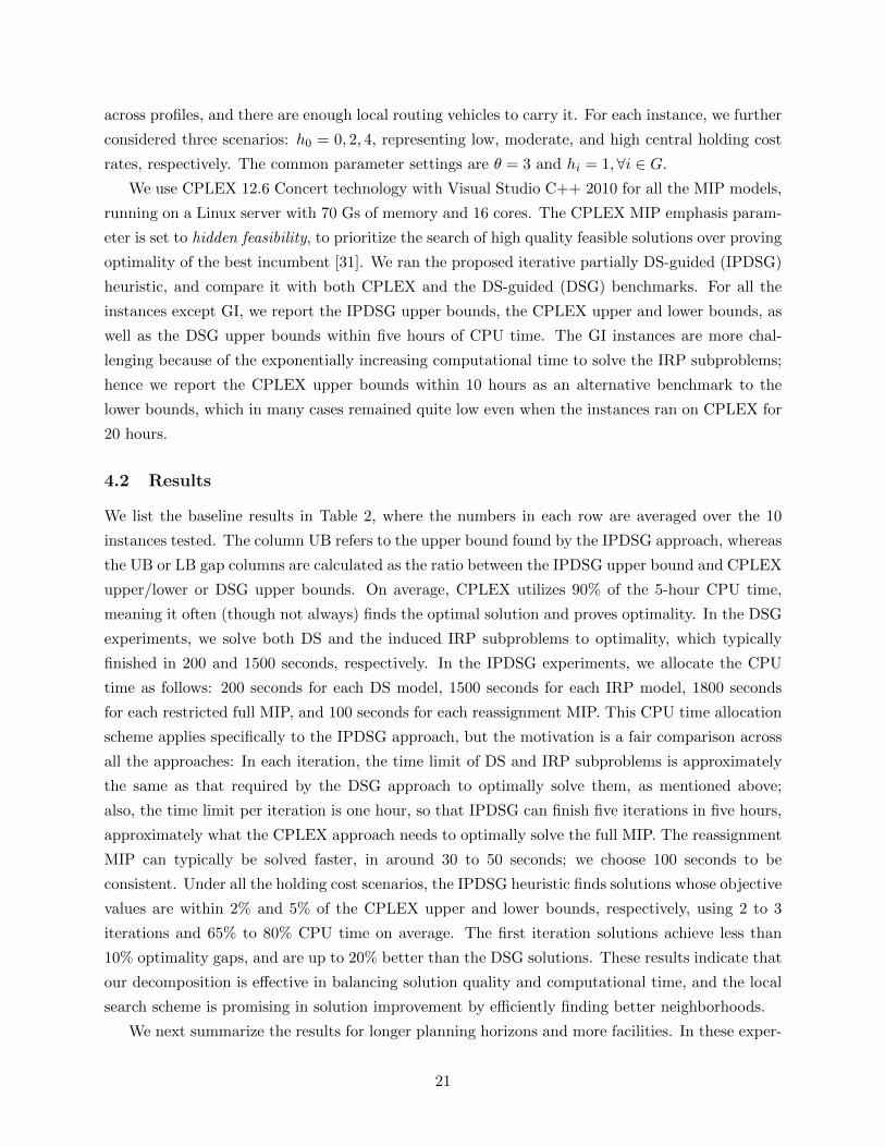
We list the baseline results in Table 2, where the numbers in each row are averaged over the 10

instances tested. The column UB refers to the upper bound found by the IPDSG approach, whereas

the UB or LB gap columns are calculated as the ratio between the IPDSG upper bound and CPLEX

upper/lower or DSG upper bounds. On average, CPLEX utilizes 90% of the 5-hour CPU time,

meaning it often (though not always) finds the optimal solution and proves optimality. In the DSG

experiments, we solve both DS and the induced IRP subproblems to optimality, which typically

finished in 200 and 1500 seconds, respectively. In the IPDSG experiments, we allocate the CPU

time as follows: 200 seconds for each DS model, 1500 seconds for each IRP model, 1800 seconds

for each restricted full MIP, and 100 seconds for each reassignment MIP. This CPU time allocation

scheme applies specifically to the IPDSG approach, but the motivation is a fair comparison across

all the approaches: In each iteration, the time limit of DS and IRP subproblems is approximately

the same as that required by the DSG approach to optimally solve them, as mentioned above;

also, the time limit per iteration is one hour, so that IPDSG can finish five iterations in five hours,

approximately what the CPLEX approach needs to optimally solve the full MIP. The reassignment

MIP can typically be solved faster, in around 30 to 50 seconds; we choose 100 seconds to be

consistent. Under all the holding cost scenarios, the IPDSG heuristic finds solutions whose objective

values are within 2% and 5% of the CPLEX upper and lower bounds, respectively, using 2 to 3

iterations and 65% to 80% CPU time on average. The first iteration solutions achieve less than

10% optimality gaps, and are up to 20% better than the DSG solutions. These results indicate that

our decomposition is effective in balancing solution quality and computational time, and the local

search scheme is promising in solution improvement by efficiently finding better neighborhoods.

We next summarize the results for longer planning horizons and more facilities. In these exper-

21

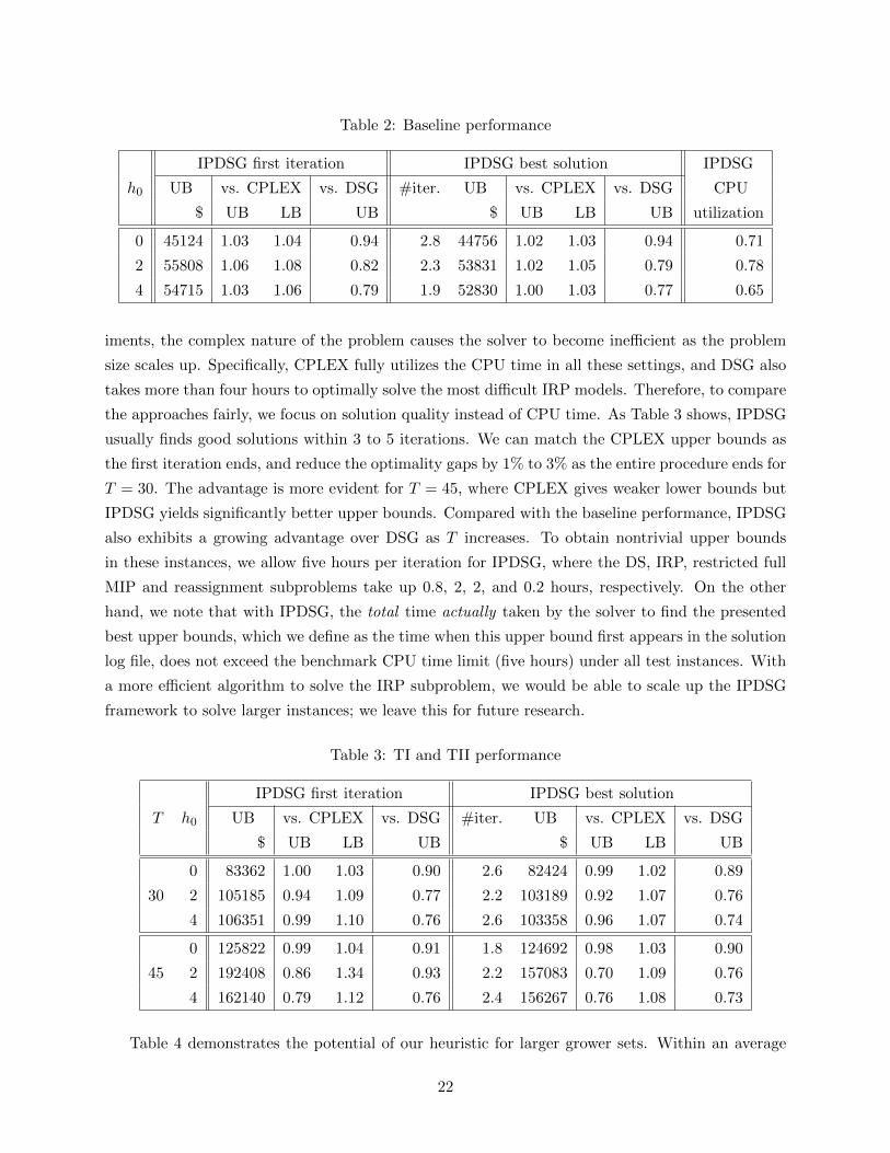
Table 2: Baseline performance

IPDSG first iteration IPDSG best solution IPDSG

h0 UB vs. CPLEX vs. DSG #iter. UB vs. CPLEX vs. DSG CPU

$ UB LB UB $ UB LB UB utilization

0 45124 1.03 1.04 0.94 2.8 44756 1.02 1.03 0.94 0.71

2 55808 1.06 1.08 0.82 2.3 53831 1.02 1.05 0.79 0.78

4 54715 1.03 1.06 0.79 1.9 52830 1.00 1.03 0.77 0.65

iments, the complex nature of the problem causes the solver to become inefficient as the problem

size scales up. Specifically, CPLEX fully utilizes the CPU time in all these settings, and DSG also

takes more than four hours to optimally solve the most difficult IRP models. Therefore, to compare

the approaches fairly, we focus on solution quality instead of CPU time. As Table 3 shows, IPDSG

usually finds good solutions within 3 to 5 iterations. We can match the CPLEX upper bounds as

the first iteration ends, and reduce the optimality gaps by 1% to 3% as the entire procedure ends for

T = 30. The advantage is more evident for T = 45, where CPLEX gives weaker lower bounds but

IPDSG yields significantly better upper bounds. Compared with the baseline performance, IPDSG

also exhibits a growing advantage over DSG as T increases. To obtain nontrivial upper bounds

in these instances, we allow five hours per iteration for IPDSG, where the DS, IRP, restricted full

MIP and reassignment subproblems take up 0.8, 2, 2, and 0.2 hours, respectively. On the other

hand, we note that with IPDSG, the total time actually taken by the solver to find the presented

best upper bounds, which we define as the time when this upper bound first appears in the solution

log file, does not exceed the benchmark CPU time limit (five hours) under all test instances. With

a more efficient algorithm to solve the IRP subproblem, we would be able to scale up the IPDSG

framework to solve larger instances; we leave this for future research.

Table 3: TI and TII performance

IPDSG first iteration IPDSG best solution

T h0 UB vs. CPLEX vs. DSG #iter. UB vs. CPLEX vs. DSG

$ UB LB UB $ UB LB UB

0 83362 1.00 1.03 0.90 2.6 82424 0.99 1.02 0.89

30 2 105185 0.94 1.09 0.77 2.2 103189 0.92 1.07 0.76

4 106351 0.99 1.10 0.76 2.6 103358 0.96 1.07 0.74

0 125822 0.99 1.04 0.91 1.8 124692 0.98 1.03 0.90

45 2 192408 0.86 1.34 0.93 2.2 157083 0.70 1.09 0.76

4 162140 0.79 1.12 0.76 2.4 156267 0.76 1.08 0.73

Table 4 demonstrates the potential of our heuristic for larger grower sets. Within an average

22

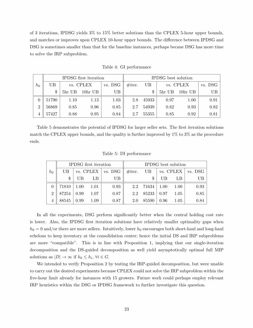
of 3 iterations, IPDSG yields 3% to 15% better solutions than the CPLEX 5-hour upper bounds,

and matches or improves upon CPLEX 10-hour upper bounds. The difference between IPDSG and

DSG is sometimes smaller than that for the baseline instances, perhaps becaue DSG has more time

to solve the IRP subproblem.

Table 4: GI performance

IPDSG first iteration IPDSG best solution

h0 UB vs. CPLEX vs. DSG #iter. UB vs. CPLEX vs. DSG

$ 5hr UB 10hr UB UB $ 5hr UB 10hr UB UB

0 51790 1.10 1.13 1.03 2.8 45933 0.97 1.00 0.91

2 56869 0.85 0.96 0.85 2.7 54939 0.82 0.93 0.82

4 57427 0.88 0.95 0.84 2.7 55355 0.85 0.92 0.81

Table 5 demonstrates the potential of IPDSG for larger seller sets. The first iteration solutions

match the CPLEX upper bounds, and the quality is further improved by 1% to 3% as the procedure

ends.

Table 5: DI performance

IPDSG first iteration IPDSG best solution

h0 UB vs. CPLEX vs. DSG #iter. UB vs. CPLEX vs. DSG

$ UB LB UB $ UB LB UB

0 71810 1.00 1.01 0.93 2.2 71634 1.00 1.00 0.93

2 87254 0.99 1.07 0.87 2.2 85233 0.97 1.05 0.85

4 88545 0.99 1.09 0.87 2.0 85590 0.96 1.05 0.84

In all the experiments, DSG perform significantly better when the central holding cost rate

is lower. Also, the IPDSG first iteration solutions have relatively smaller optimality gaps when

h0 = 0 and/or there are more sellers. Intuitively, lower h0 encourages both short-haul and long-haul

echelons to keep inventory at the consolidation center; hence the initial DS and IRP subproblems

are more “compatible”. This is in line with Proposition 1, implying that our single-iteration

decomposition and the DS-guided decomposition as well yield asymptotically optimal full MIP

solutions as |D| → ∞ if h0 ≤ hi, ∀i ∈ G.

We intended to verify Proposition 2 by testing the IRP-guided decomposition, but were unable

to carry out the desired experiments because CPLEX could not solve the IRP subproblem within the

five-hour limit already for instances with 15 growers. Future work could perhaps employ relevant

IRP heuristics within the DSG or IPDSG framework to further investigate this question.

23

5 Conclusions

In this paper, we study a two-echelon distribution problem integrating an IRP problem and a

freight consolidation problem for perishable goods with a fixed lifetime. We propose an iterative

solution framework that consists of a decomposition into subproblems and an optimization-based

local search. Extensive experiments with empirical demand distributions demonstrate the potential

of our solution approach. We also present some theoretical findings on the asymptotic behavior of

related decompositions.

The computational results motivate us to develop fast and effective heuristics for the subprob-

lems, in particular the IRP model and the restricted full MIP. We are also interested in design-

ing diversification mechanisms to explore various types of neighborhoods, which seems necessary

for larger problem instances where heuristics commonly get stuck in local optima [1, 3]. The

optimization-based local search could also give rise to simple and flexible alternatives, e.g. by in-

corporating other cost components in the objective function (7a) or revising constraints (7g)-(7h),

which would result in different reassignment strategies.

Another interesting future research direction to improve solution times for the IRP subproblem

concerns the deployment of valid inequalities within the IRP’s optimization. The use of cutting

planes and the development of branch-and-cut and branch-cut-and-price algorithms for IRP is a

growing area of interest, e.g. [2, 7, 24]. While we are not aware of any previously studied inequalities

that exactly fit our IRP model, recent results such as [11, 22, 23] suggest that adapting some classes

of cuts could help reduce solve times and allow us to solve larger models within practical time frames.

Acknowledgements

This work was partially funded by the National Science Foundation under award CMMI-1265616.

The authors thank two anonymous reviewers and the associate editor for helpful comments and

suggestions.

References

[1] N. Absi, C. Archetti, S. Dauzere-Peres, and D. Feillet. A two-phase iterative heuristic approach

for the production routing problem. Transportation Science, 49(4):784–795, 2015.

[2] Y. Adulyasak, J. F. Cordeau, and R. Jans. Formulations and branch-and-cut algorithms for

multivehicle production and inventory routing problems. INFORMS Journal on Computing,

26(1):103–120, 2014.

[3] Y. Adulyasak, J. F. Cordeau, and R. Jans. Optimization-based adaptive large neighborhood

search for the production routing problem. Transportation Science, 48(1):20–45, 2014.

24

[4] Y. Adulyasak, J. F. Cordeau, and R. Jans. The production routing problem: A review of

formulations and solution algorithms. Computers & Operations Research, 55(0):141–152, 2015.

[5] A. Akbalik and C. Rapine. Polynomial time algorithms for the constant capacitated single-

item lot sizing problem with stepwise production cost. Operations Research Letters, 40:390–397,

2012.

[6] H. Andersson, A. H. M. Christiansen, G. Hasle, and A. Løkketangen. Industrial aspects and

literature survey: Combined inventory management and routing. Computers & Operations

Research, 37(9):1515–1536, 2010.

[7] C. Archetti, L. Bertazzi, G. Laporte, and M. G. Speranza. A branch-and-cut algorithm for a

vendor-managed inventory-routing problem. Transportation Science, 41(3):382–391, 2007.

[8] C. Archetti, L. Bertazzi, G. Paletta, and M. G. Speranza. Analysis of the maximum level

policy in a production-distribution system. Computers & Operations Research, 38:1731–1746,

2011.

[9] C. Archetti, L. Bertazzi, and M. G. Speranza. Polynomial cases of the economic lot sizing

problem with cost discounts. European Journal of Operations Research, 237:519–527, 2014.

[10] V. A. Armentano, A. L. Shiguemoto, and A. Løkketangen. Tabu search with path relinking for

an integrated production-distribution problem. Computers & Operations Research, 38(8):1199–

1209, 2011.

[11] P. Avella, M. Boccia, and L.A. Wolsey. Single-Period Cutting Planes for Inventory Routing

Problems. Transportation Science, 2017. Forthcoming.

[12] J. F. Bard and N. Nananukul. Heuristics for a multiperiod inventory routing problem with

production decisions. Computers & Industrial Engineering, 57(3):713–723, 2009.

[13] J. F. Bard and N. Nananukul. The integrated production-inventory-distribution-routing prob-

lem. Journal of Scheduling, 12(3):257–280, 2009.

[14] J. F. Bard and N. Nananukul. A branch-and-price algorithm for an integrated production and

inventory routing problem. Computers & Operations Research, 37(12):2202–2217, 2010.

[15] D. E. Blumenfeld, L. D. Burns, D. J. Diltz, and C. F. Daganzo. Analyzing trade-offs between

transportation, inventory and production costs on freight networks. Transportation Research

Part B: Methodological, 19(5):361–380, 1985.

[16] M. Boudia, M. A. O. Louly, and C. Prins. A reactive GRASP and path relinking for a combined

production-distribution problem. Computers & Operations Research, 34(11):3402–3419, 2007.

25

[17] M. Boudia and C. Prins. A memetic algorithm with dynamic population management for

an integrated production-distribution problem. European Journal of Operational Research,

195(3):703–715, 2009.

[18] S. Cetinkaya. Coordination of inventory and shipment consolidation decisions: A review of

premises, models, and justification. In G. Joseph, E. Akcali, P. M. Pardalos, H. E. Romeijn,

and Z. J. Shen, editors, Applications of Supply Chain Management and E-Commerce Research,

volume 92 of Applied Optimization, pages 3–51. Springer, US, 2005.

[19] L. M. A. Chan, A. Muriel, Z. J. Shen, and D. Simchi-Levi. On the effectiveness of zero-

inventory-ordering policies for the economic lot sizing model with a class of piecewise linear

cost structures. Operations Research, 50(6):1058–1067, 2002.

[20] L. C. Coelho, J. F. Cordeau, and G. Laporte. The inventory-routing problem with transship-

ment. Computers & Operations Research, 39(11):2537–2548, 2012.

[21] L. C. Coelho, J. F. Cordeau, and G. Laporte. Thirty years of inventory routing. Transportation

Science, 48(1):1–19, 2014.

[22] L.C. Coelho and G. Laporte. Improved Solutions for Inventory-Routing Problems through

Valid Inequalities and Input Ordering. International Journal of Production Economics,

155:391–397, 2014.

[23] G. Desaulniers, J.G. Rakke, and L.C. Coelho. A Branch-Price-and-Cut Algorithm for the

Inventory Routing Problem. Transportation Science, 50:1060–1076, 2016.

[24] F. G. Engineer, K. C. Furman, G. L. Nemhauser, M. W. P. Savelsbergh, and J. H. Song.

A branch-price-and-cut algorithm for single-product maritime inventory routing. Operations

Research, 60(1):106–122, 2012.

[25] M. Florian, J. K. Lenstra, and A. H. G. Rinnooy Kan. Deterministic production planning:

Algorithms and complexity. Management Science, 26(7):669–679, 1980.

[26] F. Fumero and C. Vercellis. Syncronized development of production, inventory, and distribution

schedules. Transportation Science, 33:330–340, 1999.

[27] M. Goetschalckx. Supply Chain Engineering. Springer, London, 2011.

[28] R. W. Hall. Consolidation strategy : Inventory, vehicles and terminals. Journal of Business

Logistics, 8(2):57–73, 1987.

[29] W. Hu. Modeling and Solution of Some Multi-Period Supply Chain Optimization Problems.

PhD thesis, Georgia Institute of Technology, 2016.

26

[30] W. Hu, A. Toriello, and M. Dessouky. Decomposition-based approximation algorithms for the

one-warehouse multi-retailer problem with concave batch order costs. Working paper, available

at http://www2.isye.gatech.edu/~atoriello3/owmr_apx.pdf, 2016.

[31] IBM ILOG. CPLEX Optimization Studio CPLEX Parameters Reference, version 12.6.

Available at http://www.ibm.com/support/knowledgecenter/SSSA5P_12.6.3/ilog.odms.

studio.help/pdf/paramcplex.pdf.

[32] Y. Jin and A. Muriel. Single-warehouse multi-retailer inventory systems with full truckload

shipments. Naval Research Logistics, 56(5):450–464, 2009.

[33] S. A. Lippman. Optimal inventory policy with multiple set-up costs. Management Science,

16(1):118–138, 1969.

[34] C. Nguyen, M. Dessouky, and A. Toriello. Consolidation strategies for the delivery of perishable

products. Transportation Research Part E: Logistics and Transportation Review, 69:108–121,

2014.

[35] C. Nguyen, A. Toriello, M. Dessouky, and J. E. Moore. Evaluation of transportation practices

in the california cut flower industry. Interfaces, 43(2):182–193, 2013.

[36] D. J. Papageorgiou, G. L. Nemhauser, J. Sokol, M.-S. Cheon, and A. B. Keha. MIRPLib – A

library of maritime inventory routing problem instances: Survey, core model, and benchmark

results. European Journal of Operational Research, 235(2):350 – 366, 2014.

[37] M. Ruokokoski, O. Solyalı, R. Jans, and H. Sural. Efficient formulations and a branch-and-

cut algorithm for a production-routing problem. GERAD Technical Report G-2010-66, HEC

Montreal, Canada, 2010.

[38] O. Solyalı and H. Sural. A relaxation based solution approach for the inventory control and

vehicle routing problem in vendor managed systems. In S. K. Neogy, A. K. Das, and R. B.

Bapat, editors, Modeling, Computation and Optimization, volume 6 of Statistical Science and

Interdisciplinary Research. World Scientific, Singapore, 171-189, 2009.

[39] G. Stauffer, G. Massonnet, C. Rapine, and J.-P. Gayon. A simple and fast 2-approximation

algorithm for the one-warehouse multi-retailer problem. In Proceedings of the Twenty-Second

Annual ACM-SIAM Symposium on Discrete Algorithms, pages 67–79, 2011.

[40] U.S. Department of Agriculture and U.S. Department of Transportation. Study of rural trans-

portation issues. Technical report, Washington DC, April 2010.

27

Appendix A Remaining Proofs

A.1 Proof of Proposition 1

We bridge the specified DS-guided solution and the optimal full MIP solution with an auxiliary

solution, which is constructed as follows:

Step 1. Solve the DS subproblem with h0,i to obtain the long-haul shipping decisions.

Step 2. For each grower i ∈ G, assign the associated DS shipping quantities to the commodity

ready periods for local pickup if its holding cost rate exceeds the warehouse’s rate; otherwise,

assign those quantities to the DS shipping periods. That is, add constraints qsm + vsm = dm

in the IRP subproblem if hi > h0, else add qt−1m + vt−1m =∑

p∈{F,L,U} ztmp, ∀m ∈ M ·i·, t =

(s + 1) . . .min{s + θ, T}, where ztmp are the values determined in Step 1. This gives the

system-wide inventory decisions.

Step 3. Solve the resulting IRP subproblem to obtain the short-haul shipping decisions.

The above procedure yields a feasible full MIP solution. Let the overall costs for this solution, the

specified DS-guided solution and the optimal full MIP solution be Za, ZDSG and Z∗, respectively.

Using the same superscripts, let V ·, H · and C · be the respective total local vehicle routing and

alternative direct shipping cost, total system-wide holding cost, and total long-haul direct shipping

cost incurred by the corresponding full MIP solutions, i.e. Z · = V ·+H ·+C ·. Assume the demand

for each commodity, dm, is i.i.d. in each period with mean dik > 0, ∀m ∈ M ·ik. We will show that

lim|D|→∞ZDSG−Z∗

Z∗ = lim|D|→∞Za−Z∗Z∗ = 0 with probability 1.

First, ZDSG ≤ Za: We respect the DS-guided long-haul shipping plan when constructing the

auxiliary solution; hence CDSG = Ca. The auxiliary solution implies a feasible solution to the

IRP subproblem induced by the DS-guided decomposition under the same long-haul shipping plan;

hence HDSG + V DSG ≤ Ha + V a.

Second, Ha + Ca ≤ H∗ + C∗: Step 2 ensures that the total system-wide holding cost and

long-haul shipping cost incurred by the auxiliary solution equals the optimal objective value of the

DS subproblem under the revised holding cost rates h0,i, which is in fact a relaxation of the full

MIP where the local transportation decisions x, y, u are removed. The relaxation can be validated

by converting any given feasible full MIP solution into a feasible solution with no higher objective

value for the specified DS subproblem analogously to Step 2; see [30] Lemma 8.2 and [39] Lemma

5.1 for more details on relevant two-echelon inventory models.

Third, V a − V ∗ ≤ T |G|(A + B), where A is the optimal TSP tour cost when all growers are

visited, and B the per alternative local direct shipment cost parameter (see §2). This is true since

we allow one routing vehicle in each period, and the alternative direct shipments contain at most

one partially-filled truck for each grower in each period.

Fourth, C∗ ≥∑

k∈D∑

m∈M ··kckFdm/KF , where the right-hand-side is the long-haul direct ship-

ping cost with the highest possible truck capacity utilization. This value is obtained by assuming

28

the lowest possible unit rates of ckF /KF and the longest possible product lifetime θ = T ; hence it

is a lower bound for that incurred by any feasible full MIP solution.

Therefore, ZDSG−Z∗Z∗ ≤ Za−Z∗

Z∗ ≤ V a−V ∗C∗ ≤ T |G|(A+B)∑

k∈D∑m∈M··k

ckF dm/KF → 0 as |D| → ∞. In other

words, both the auxiliary solution and the specified DS-guided solution are asymptotically optimal

when there are arbitrarily many sellers.

The proposition can be extended to the case of multiple local routing vehicles by slightly mod-

ifying the comparison of V a and V ∗ assuming B ≤ A.

A.2 Proof of Proposition 2

We show the result with the following lemmas. Lemma 3 ensures the existence of a special cost func-

tion that bounds each seller’s long-haul transportation cost function from above, whereas Lemma

4 gives structural properties of an LSP under this upper bound cost function. Both lemmas are

proved in [29].

Lemma 3. Let Ck(q) be the long-haul direct shipping transportation cost when q units are sent to

retailer k. There exist functions Ck(·) such that

Ck(q) ≤ Ck(q) = b qKFc · ckF + ck(q mod KF ), ∀q ∈ R+, (8)

where ck(·) is a PWL concave function on [0,KF ] and ck(KF ) = ckF , ∀k ∈ D.

Lemma 4. The perishable lot sizing problem with concave batch transportation costs, where the

item lifetime is fixed and the cost per batch is an identical concave function of the shipping volume

within the batch capacity, has an optimal solution such that in each period,

i) there is at most one partially filled batch;

ii) the end inventory is lower than the batch capacity.

Let Z∗ and ZIRPG be the optimal full MIP objective value and that of the IRP-guided solution,

respectively. When the IRP subproblem is solved with h′0 = 0, it minimizes the short-haul trans-

portation costs and the grower holding costs under any input cost parameters; hence its objective

value does not exceed the corresponding cost components of the optimal full MIP solution. To

analyze the gap between ZIRPG and Z∗, it then suffices to check the central inventory costs and

the long-haul transportation costs. Let W ∗, W IRPG, and W IRPG be the respective total values of

these cost components incurred by the optimal full MIP solution, the IRP-guided solution, and the

optimal solution of the DS subproblem which uses the central supply implied by the IRP solution

and some Ck(·) that satisfy (8). Since the long-haul decision for each seller is independent from the

others’ under the given central supply, the DS subproblem is equivalent to |D| lot sizing problems.

Applying a similar argument as Theorem 7.1 in [32], we have

ZIRPG − Z∗

Z∗≤ W IRPG −W ∗

W ∗≤ W IRPG −W ∗

W ∗≤

∑k∈D(h0KF + ckF )T∑

i∈G∑

k∈D∑

m∈M ·ikckFdm/KF

, (9)

29

where W IRPG ≤ W IRPG is implied by Lemma 3; W ∗ ≥∑

i∈G∑

k∈D∑

m∈M ·ikckFdm/KF since the

right-hand-side number is the lowest possible long-haul transportation cost assuming the highest

truck capacity utilization, which also gives W IRPG−W ∗ ≤∑

k∈D(h0KF + ckF )T by Lemma 4. Let

the demand for each commodity in each period dm be i.i.d. with mean dik > 0, ∀i ∈ G, k ∈ D,m ∈M ·ik; then

∑k∈D(h0KF + ckF ) ∼ o(

∑i∈G

∑k∈D

∑m∈M ·ik

ckFdm/TKF ) with probability 1, and the

right-hand side of (9) converges to 0 as |G| → ∞.

30