Computer Vision and Image Understanding 113 (2009) 708–725

Contents lists available at ScienceDirect

Computer Vision and Image Understanding

journal homepage: www.elsevier .com/locate /cv iu

Integrated detection and tracking of multiple faces using particlefiltering and optical flow-based elastic matching

Suchendra M. Bhandarkar *, Xingzhi LuoDepartment of Computer Science, The University of Georgia, Athens, GA 30602-7404, USA

a r t i c l e i n f o a b s t r a c t

Article history:Received 30 August 2006Accepted 26 November 2008Available online 21 January 2009

Keywords:Particle filteringMultiple face trackingGenetic AlgorithmElastic matchingOptical flow

1077-3142/$ - see front matter � 2008 Elsevier Inc. Adoi:10.1016/j.cviu.2008.11.010

* Corresponding author.E-mail address: suchi@cs.uga.edu (S.M. Bhandarka

The design and implementation of a multiple face tracking framework that integrates face detection andface tracking is presented. Specifically, the incorporation of a novel proposal distribution and object shapemodel within the face tracking framework is proposed. A general solution that incorporates the mostrecent observation in the proposal distribution using a multiscale elastic matching-based optical flowalgorithm is proposed. The proposed multiscale elastic matching-based optical flow algorithm is shownto be general and powerful in three significant ways. First, it allows for the tracking of both, rigid andelastic objects. Second, it enables robust tracking even in the face of sudden and gradual changes in illu-mination, scale and viewpoint. Third, it is suitable for tracking using both, fixed cameras and movingcameras. The proposed object shape model is based on a kernel-based line segment matching algorithm,which incorporates a voting scheme similar to the Radon Transform. The incorporation of the objectshape model is shown to improve the computational complexity and accuracy of the face tracking algo-rithm and also enhance its robustness to occlusion, noise and scene clutter. Efficient techniques for par-ticle sampling based on the Genetic Algorithm and for computation of the region-based likelihoodfunction using the integral image are proposed. The incorporation of face detection within the face track-ing algorithm is also proposed. Experimental results show that the proposed face tracking system is veryrobust in its ability to handle occlusion, noise, scene clutter and changes in illumination, scale and view-point and is also computationally efficient.

� 2008 Elsevier Inc. All rights reserved.

1. Introduction

Computer vision-based tracking of multiple objects is challeng-ing in several aspects. The first challenge arises from occurrence ofocclusion, including mutual occlusion between foreground objectsand occlusion caused by background objects, which makes it diffi-cult to accurately localize the occluded object and track it contin-uously. The second challenge is the formulation of an objectmodel that is able to capture important and relevant informationabout the tracked object in order to facilitate fast and reliabletracking even in the face of occlusion. The third challenge is tobe able to accurately predict/estimate the object position and up-date the prediction via accurate localization. The fourth challengeis to meet the real time constraints of most tracking applicationsin the real world. Accurate and robust object localization in realtime over several video frames is the ultimate objective of a real-world tracking system.

Factors such as measurement noise, inaccurate object modeling,changes in illumination, scale and viewpoint, scene clutter, false tar-gets (positives) and instances of occlusion contribute towards the

ll rights reserved.

r).

uncertainty in the state (location, identity, velocity, shape etc.) ofthe tracked object. This necessitates a stochastic Bayesian trackingframework as opposed to a deterministic one. In a Bayesian tracker,the current state of the tracker is denoted by Xt whereas the currentobservation (image frame) is represented by the variable It . The goalof a Bayesian tracker is to recursively estimate the current filteringor posterior distribution pðXt jI1:tÞ given the observation likelihooddistribution pðIt jXtÞ, the state transition prior distributionpðXt jXt�1Þ and the previously estimated filtering (posterior) distri-bution pðXt�1jI1:t�1Þwhere I1:t denotes the sequence of observations(image frames) fI1; I2; . . . ; Itg. The recursive Bayesian estimation pro-cedure is given by the following pair of equations:

pðXtjI1:t�1Þ ¼Z

pðXt jXt�1ÞpðXt�1jI1:t�1ÞdXt�1 ð1Þ

and

pðXtjI1:tÞ ¼pðItjXtÞpðXtjI1:t�1Þ

pðItjI1:t�1Þð2Þ

The recursive Bayesian estimation procedure in Eqs. (1) and (2) rep-resents the propagation of the tracking hypothesis frompðXt�1jI1:t�1Þ to pðXtjI1:tÞ. The prediction (Eq. (1)) involves high-dimen-sional integration and is difficult to solve analytically. Consequently,

S.M. Bhandarkar, X. Luo / Computer Vision and Image Understanding 113 (2009) 708–725 709

the filtering distribution pðXtjI1:tÞ is approximated by a set ofweighted particles fðXi

t;witÞ : i ¼ 1; . . . ;ng, where n is the number of

particles, t is the time variable and wit is the weight of particle Xi

t , usinga sampling importance resampling (SIR) procedure. Each particleXi

t ¼ ðoi1; . . . ; oi

mÞ represents a specific configuration of the tracked ob-jects oi

k, 1 6 k 6 m, where m is the number of objects, and is termed asa tracking hypothesis. The object description oi

k consists of, typically,its identity, location, velocity, shape, color and other features of inter-est. In the SIR procedure the proposal distribution pðXtjX1:t�1; I1:tÞ isused to approximate the filtering distribution pðXtjI1:tÞ since samplingdirectly from the latter is often not feasible. The proposal distributionin turn is simplified as pðXtjX1:t�1; I1:tÞ � pðXtjX1:t�1Þ � pðXtjXt�1Þusing the Markovian property. Thus, the proposal distribution isapproximated by the state transition prior distribution pðXtjXt�1Þand the weight of the particle Xi

t is computed as wit � pðIt jXi

tÞ. Theresulting approximation to the recursive Bayesian estimation proce-dure is termed as the particle filter which has proven to be a very effec-tive technique for object tracking.

A typical particle filter-based tracker is composed of three basiccomponents. The first component is the statistical object model,which is used to compute the likelihood distribution pðIt jXi

tÞ ofeach particle Xi

t , where It is the current observation (image frame).The second component is the sampling algorithm, which computesa set of new particles fXi

t

0g from a set of existing particles fXi

tg, i.e.,fXi

t

0g ¼ fSðfXi

tgÞ, where fS is the sampling algorithm. Most particlefiltering algorithms sample the particles in direct proportion tothe posterior probability of each particle pðXi

tjItÞ which is typicallyapproximated by the state transition prior distribution pðXt jXt�1Þ.The third component is the transition function Xi

t ¼ fTðXit�1; ItÞ,

which computes the new parameters of a configuration Xit when

the current observation It and the previous configuration Xit�1 are

given. The transition function is essentially derived from the pro-posal distribution or an approximation thereof. Linear predictionis usually used as the transition function in conventional particlefilters [14]. The particle filtering algorithm works iteratively as fol-lows: (a) Initialize the particles fXi

0;wi0g and compute their likeli-

hood distributions wi0 ¼ pðI0jXi

0Þ; (b) Sample the current set ofparticles to generate a new particle set using the sampling algo-rithm fXi

t�1

0g ¼ fSðfXi

t�1gÞ; and (c) Given the new observation It , ap-ply transition function fTð:Þ to generate the new sample setfXi

tg ¼ fTðfXit�1

0g; ItÞ and update the weight of each particle Xi

t .The traditional particle filter [12,14] has been used successfully

in several computer vision-based tracking applications. However,as elaborated upon in Section 3, the traditional particle filter suf-fers from certain key shortcomings when dealing with tracking ofmultiple objects in the presence of occlusions and scene clutter.

2. Brief literature review

Generally speaking, there exist three broad categories of objectmodels in the context of tracking: contour-based models[2,16,19,24,36], region-based models [7,10,14,25,28,34], and fea-ture point-based models [18,22,32]. The absence of color or edgeinformation from within the interior of the object, restricts theability of contour-based models to handle occlusion. Most re-gion-based models exploit the color distribution within the trackedobject, allowing for computationally efficient tracking [7,25,28].The use of kernel functions and a similarity measure between colordistributions [7] allows for robust tracking in the face of occlusion.However, it is not possible to achieve accurate tracking in multi-ple-object scenes when the color distributions within different ob-jects are similar. A grid-based object model [14,34] can potentiallyencode more detailed spectral (color) and structural (shape) infor-mation of the tracked objects but the encoding of the shape infor-mation is sensitive to the structural organization of the grid [14].

Feature point-based tracking is popular on account of its sim-plicity and relative ease of encoding object shape informationusing corner points [11,18,22] or edge points [26,32] as the featurepoints of interest. However, feature point-based tracking methodsare easily distracted by noisy feature points in the background andare, by their very nature, limited to objects rich in feature points.When the image regions that correspond to the tracked objectsare largely homogeneous, few salient feature points are availablethus causing the robustness of the tracking to suffer. Hybrid objectmodels [3,6] that encode both boundary and region informationare attractive since they potentially provide the desired robustnessto occlusion. However, current hybrid models [3] are computation-ally too intensive and hence unacceptable for real-time surveil-lance applications.

The CONDENSATION tracker [12,14] represents one of the earlyparticle filter implementations of the recursive Bayesian trackingparadigm using the SIR procedure. More recent implementationsof the particle filter have focussed on improving the estimationof the proposal distribution and formulation of the transition func-tion. The simplified proposal distribution in the conventional par-ticle filter [12,14] uses only historical data to predict the newstatus of Xt . In the interest of simplicity of the analytical formula-tion, the current observation It is ignored in the estimation of theproposal distribution and the transition function even when it isavailable. However, to ensure robustness, it is important to incor-porate the most current observation It in the proposal distributionsince ignoring it makes the system susceptible to failure whentracking fast moving objects. Recent approaches to incorporate It

in the proposal distribution include the design of an an auxiliarytracker [13] and the use of a Kalman filter resulting in a KalmanParticle Filter (KPF) or Unscented Kalman Particle Filter (UKPF)[19]. However, the auxiliary tracker itself needs a good proposaldistribution thus presenting a chicken-and-egg problem, whereasthe Kalman filter entails the formulation of an observation functionwhich is unavailable, inaccurate or highly sensitive to randomnoise and occlusion in the image [19].

The particle filter has also been extended to address the prob-lem of tracking multiple objects. In the Boosted Particle Filter(BPF) [29], the Adaboost detection algorithm [39] is interleavedwith a Gaussian mixture-based particle filter. The multiple-objecttracking hypothesis is modeled using a mixture of independentGaussian distributions supported by a common set of particles,where each tracked object is represented by a component of theGaussian mixture. The assumption regarding the independence ofthe Gaussian mixture components, however, breaks down whenthe multiple objects move together (i.e., exhibit correlated mo-tion). Also, the modified proposal distribution in the BPF is mod-eled as a weighted linear combination of the Adaboost proposaldistribution and the proposal distribution of the Gaussian mix-ture-based particle filter. This raises certain critical issues, namely,how does one assign weights to the individual proposal distribu-tions in the above weighted linear combination and how doesone interpret the results when the means of the individual pro-posal distributions are separated significantly. The BPF also suffersfrom the correspondence problem, i.e., it is difficult to determinethe set of particles that correspond to a specific tracked object.The BRAMBLE multiple-object tracking algorithm [14] which ran-domly generates a new object and removes an existing object usinga Poison distribution model, is also seen to suffer from the afore-mentioned correspondence problem.

3. Contributions of the paper

The accuracy, robustness and computational efficiency of themajor components, i.e., the object model, particle sampling proce-

Fig. 1. Proposed System for Integrated Object Detection and Object Tracking.

710 S.M. Bhandarkar, X. Luo / Computer Vision and Image Understanding 113 (2009) 708–725

dure, proposal distribution and transition function, are critical foran effective particle filter-based tracking system. In this paper wepresent four significant enhancements to the conventional particlefilter that enhance the accuracy, robustness and computationalefficiency of the aforementioned components, namely, (a) an im-proved proposal distribution and transition function that entailthe computation of optical flow using a multiscale elastic matchingalgorithm, (b) an improved object model that integrates a statisti-cal region-based model and a statistical shape-based model, (c) animproved particle sampling procedure based on the Genetic Algo-rithm (GA) and (d) incorporation of object detection within objecttracking which alleviates the common problems associated withextending the particle filtering framework to a multiple objecttracking scenario. These enhancements are further detailed in theremainder of this section.

The proposal distribution proposed in this paper is unique inthat the current observation is incorporated by exploiting the opti-cal flow and velocity field to update the state(s) of the particles.Inaccurate prediction of the object location by the proposal distri-bution and transition function results in a large number of particlesrequired to support the tracking hypothesis on account of thegreater uncertainty in object localization. Our previous work [21]has shown that the imposition of spatial constraints on the opticalflow field enables the tracking of multiple objects in complex situ-ations with just a single tracking hypothesis. However, a majorshortcoming of a single hypothesis-based multiple object trackeris its propensity to get trapped in a local optimum in spite of theincorporation of optical flow information [21]. Consequently, inthe proposed tracking algorithm, we incorporate optical flow infor-mation within a multiple tracking hypothesis framework. The opticalflow and velocity field are used to predict the new locations of theparticles accurately and efficiently. In the case of partially occludedobjects, the imposition of spatial constraints is shown to enableaccurate computation of the velocity field in the unoccluded re-gions of the image, which in turn allows the tracking parametersof partially occluded objects to be correctly updated. It is shownthat incorporation of multiscale elastic matching and use of mul-ti-spectral channels within the optical flow computation enablesthe tracking algorithm to deal with object shape deformation,and changes in scale, viewpoint and illumination. Unlike the KPF[19], the proposed optical flow computation does not require anaccurate measurement function thus making it more general androbust than the KPF.

The proposed object model is based on the integration of a sta-tistical region model and a statistical shape model. It is designed tomake the tracker computationally efficient, enhance its robustnessto noise, clutter and occlusion, and increase the tracking accuracyby reducing the variance or uncertainty associated with the track-ing parameters. The proposed object model enables more accurateestimation of the likelihood pðIt jXtÞ compared to simpler region-based models even in instances of partial occlusion [29,38]. Thestatistical region model is trained on human skin color to enablehuman face detection and tracking. The region-based log-likeli-hood measure is based on region (skin) color and computed effi-ciently using an integral image [40,41]. The statistical shapemodel within the proposed object model relies on a line segmentmatching procedure similar to the one used in structural indexing[33] and geometric hashing methods [9,42] for object recognition.In contrast to the computationally intensive edge-based statisticalshape model proposed in [3], the proposed line segment matchingprocedure is shown to produce a smooth probability surface for theshape model in a computationally efficient manner using a kernel-based voting scheme similar to that used in the Radon Transform[8,37]. The kernel-based voting scheme is restricted to the compu-tation of the shape likelihood function via precomputation andindexing of the line segments using a simple hash table. The like-

lihood of each instance of the shape model in the image is com-puted efficiently without having to compute the probabilitydistribution function over the entire parameter space as in the caseof the Radon Transform. The proposed kernel-based voting schemeis shown to be robust in the presence of occlusion. The incorpora-tion of the shape model within the particle filter is shown to resultin a more compact distribution of the resulting particles (i.e., withlower variance). It should be noted that although the efficacy of theproposed object model is demonstrated in the context of facedetection and face tracking, the overall object modeling frameworkcan be applied to the detection and tracking of general objects forwhich appropriate statistical region and shape models can beformulated.

The proposed sampling procedure for the particle filter incorpo-rates elements of the Genetic Algorithm (GA) [27] within the con-ventional SIR procedure of the CONDENSATION tracker [12,14]. In amultiple-object tracking scenario, the GA is shown provide a natu-ral mechanism for retaining particles that better support the track-ing hypothesis while eliminating those that do not. In particular,the crossover operator in the GA is shown to improve the probabil-ity of finding a good multiple-object configuration hypothesis (i.e.,one with higher likelihood) thus enabling the sampling procedureto converge faster and on a more accurate set of trackinghypotheses.

The final enhancement is the incorporation of an explicit objectdetection and validation procedure within the proposed trackingframework. This ensures that each particle represents an identicalnumber of tracked objects and that the ith object in particle m1 cor-responds to the ith object in particle m2. Thus, each particle de-notes a distinct multiple-object hypothesis and represents thesame set of objects in the scene. This circumvents the correspon-dence problem and the independence assumption problem dis-cussed previously in the context of the BPF [29] and theBRAMBLE tracker [14].

Fig. 1 depicts the proposed tracking framework which inte-grates object detection with the proposed multiple-object trackingalgorithm. The tracking algorithm tracks the location of each objectin the new image whereas the detection algorithm detects thepresence of new objects. The validation algorithm uses the proba-bilistic object model and occlusion reasoning to validate the pres-ence of new and previously tracked objects. Although the proposedscheme is currently implemented for the detection and tracking of(multiple) human faces in video streams, it is general enough to beused for the detection and tracking of any object for which appro-priate region- and shape-based models can be formulated. The factthat the efficacy of the proposed scheme is demonstrated in thecontext of detection and tracking of (multiple) human faces in vi-deo streams does not diminish the generality of the underlyingformulation.

The proposed system can be briefly described as follows. Givena new image and the set of n particles fXi

tg:

(1) The log-likelihood values of the face (skin) color distributionpðyjFÞ and non-face color distribution pðyjFÞ at each pixel loca-tion y are computed using a log-likelihood lookup table. These

S.M. Bhandarkar, X. Luo / Computer Vision and Image Understanding 113 (2009) 708–725 711

values are then used to compute the region log-likelihood valueof each particle. The line segments describing the object shapeare extracted and indexed, and used to compute the shapeprobability of each instance of the object for each particle.

(2) The proposed transition function that incorporates multi-scale elastic matching-based optical flow computation isused to compute the new parameters of each particle Xi

t

0.

(3) The object detection algorithm is used to detect the presenceof new objects. If a new object oi is detected, n new instancesof object oi are generated based on the location of thedetected object. Each of the n particles Xi

t is updated by hav-ing an instance of object oi appended to it.

(4) The log-likelihood of each particle logðpðIjXit

0ÞÞ is computed

based on the region- and shape-based object model.(5) The output particle set is computed using a weighted aver-

aging algorithm.(6) The output is validated and occlusion reasoning is per-

formed. Invalid objects are removed from consideration.(7) The new set of particles is generated for the next iteration

using a novel combination of the traditional SIR procedureof the CONDENSATION tracker [12,14] and a GA [27]. Thetracking algorithm proceeds to step 1 of the next iteration.

The remainder of the paper is organized as follows. Section 4describes briefly the proposed object model wherein Section 4.1details the proposed region-based model and Section 4.2 detailsthe proposed shape model. Section 5 details the computation ofthe configuration probability or particle likelihood via integrationof the shape model and region model. Section 6 describes the pro-posed sampling algorithm which incorporates the GA [27] withinthe SIR procedure of the CONDENSATION tracker [12,14]. Section7 describes the proposed proposal distribution which is based onthe computation of optical flow using multiscale elastic matching.Section 8 summarizes the proposed system. Section 9 presentsexperimental results in the context of detection and tracking ofmultiple human faces in fairly complex scenes containing in-stances of occlusion, scene clutter and changes in illumination,scale and viewpoint. Section 10 concludes the paper with an out-line for future work.

4. Object representation

In the proposed tracking scheme, a particle denotes a trackinghypothesis, i.e., a configuration of the foreground objects at any gi-ven instant of time. A particle Xi

t is represented as a vector whereeach component of the vector denotes the individual state of a dis-tinct foreground object. Each foreground object oi

j is associatedwith a contour c and a region r. Consequently, particleXi

t ¼ ðoijðc; rÞÞ, j ¼ 1; . . . ;m, where m is the number of tracked ob-

jects at time t. Each object oij is represented as a vector of parame-

ters ðx; y; h; s; idÞ, where ðx; yÞ is the centroid of the object, id is thetemplate identification number, s is the scale, and h is the rotationangle. That is, each object is expressed as a 2-D Euclidean transfor-mation of one of the shape templates where the contour c auto-matically determines the region r.

4.1. Region-based object model

A color-based region model is proposed for the human face andused to compute efficiently the log-likelihood value of each face re-gion using the integral image and the union set operator. Based onthe independence assumption, the log-likelihood computation isrepresented as a summation of feature-based log-likelihood valuesat each pixel within the region. Each object region is represented asa simple rectangle or a combination of rectangles. A 2-D integral

image [40,41] is used to speed up the log-likelihood computationsince the summation of the log-likelihood values in a rectanglecan be computed with two additions and one subtraction. Sincethe feature vector at each pixel is multi-dimensional, the integralhistogram algorithm presented in [31] is used to compute the inte-gral image. The major difference between the proposed integralimage approach and the approaches described in [40] and [41] isthat, in our case, the integral image is defined over the pixel valuesof the log likelihood image whereas in [40] and [41] it is definedover the grayscale or color histogram of the image pixels.

In the proposed integral image approach, overlapping rectan-gles need to be given special consideration since the simple addi-tion of the log-likelihood values of two overlapping rectangleswould yield an incorrect result. A particle is represented as an ar-ray of foreground objects Xr ¼ ðo1; . . . ; omÞ where each foregroundobject is represented by a set of rectangular regions fr1; . . . ; rgg.For each region rj, the summation of its pixel log-likelihood valuesis denoted by Lrj

. If the regions rj are non-overlapping, then the to-tal log-likelihood Lr is given simply by Lr ¼

PLrj

. However, whenthe regions rj are overlapping, the simple summation will countsome regions more than once, and hence give incorrect results. Gi-ven a set of regions R ¼ fr1; . . . ; rgg, we define the region setRk ¼ fra1 \ . . . \ rak

; aj 2 ½1; . . . ; g�;8i; j; ai < aj () i < jg. We also de-fine

Sk ¼

PR2Rk

R, then the regionSg

1ri ¼S

1 �S

2 þS

3 � . . . :

þð�1Þkþ1Sk and the corresponding likelihood value is given by

L[g

1

ri

!¼ L

[1

!� L

[2

!þ L

[3

!� . . .þ ð�1Þkþ1L

[k

!ð3Þ

For example, the union of three sets A;B; C can be computed asA [ B [ C ¼ Aþ Bþ C � ðA \ BÞ � ðA \ CÞ � ðB \ CÞ þ ðA \ B \ CÞ andthe corresponding likelihood computed as LðA [ B[CÞ ¼ LðAÞ þ LðBÞþ LðCÞ � LðA \ BÞ� LðA \ CÞ � LðB \ CÞ þ LðA \ B \ CÞ.

4.2. Shape-based object model

A contour-based model of the object shape is used where theobject contours are approximated by a sequence of connected linesegments. A contour-based model was observed to be less sensitiveto noise and outliers than the edge pixel-based shape model de-scribed in [3]. The line segment-based contour approximation alsoallows for more efficient computation of the affine transformationand similarity matching of the line segments than B-splines or Be-zier curves that could potentially yield a better approximation tothe object contours.

The matching algorithm for computing shape similarity is basedon a geometric hashing procedure described in [9,42] and uses avoting procedure similar to the one used in the Radon Transform[8,37] for shape recognition. The Radon Transform, which can beviewed as a general procedure to map a set of image observations(edge pixels, line segments, ...) to a parametric description of theobject shape, is known to be capable of handling instances of occlu-sion and missing data in the image. The Radon Transform typicallyentails an exhaustive search of the parameter space and is hencecomputationally intensive, especially when dealing with largeparameter spaces. In the proposed tracking framework, we areinterested primarily in computing the conditional probabilitypðIt jStÞ of the current image It for a given set of shape instancesSt ¼ fSi

t ; 1 6 i 6 mg with known shape parameters, rather thanfor all possible shapes, where m is number of tracked objects.Hence we compute the conditional probability specifically for theexisting shape instances described by the current set of particles,rather than for the entire parameter space. All possible line seg-ments for the current image are computed using an incrementalline segment approximation algorithm and stored in a hash table.The hash table allows for efficient computation of the shape prob-

712 S.M. Bhandarkar, X. Luo / Computer Vision and Image Understanding 113 (2009) 708–725

ability whereas the proposed probabilistic shape model ensuresthat the resulting probability surface is smooth.

In the proposed shape model, the line segments are first ex-tracted from the observed image using algorithms for edge detec-tion and line segment following. The extracted line segments arethen used to vote for the object shapes. The shape model is pre-trained using the clustering algorithm described in Section 5.2.1,from which a set of shape templates fSi; i ¼ 1; . . . ; Tg is obtained.A shape template is given by Si ¼ fEi;j ¼ ðCi;j;Hi;j; Li;jÞ;rC;i;

rH;i;rL;i; j ¼ 1; . . . ;Mg, where Ci;j is the center, Hi;j the angular ori-entation and Li;j the length of the line segment. The parametersrC;i;rH;i and rL;i are the standard deviations of C;H and L, respec-tively. When we compute the line segment approximations to theshape templates, we ensure that the lengths of the line segmentsare approximately equal and the number of line segments M isidentical for all shape templates. This simplifies the matching algo-rithm designed to compute the shape probability.

Each shape template is associated with a prior distribution pðSiÞ.The time series of the shapes is assumed to be a Markov process, thatis pðSt jSt�1; . . . ; S0Þ ¼ pðSt jSt�1Þ. With this simplification, pðStjSt�1Þcan be precomputed easily with training data. The shape probabilitymodel is used subsequently in the sampling procedure of the particlefilter. However, before presenting the algorithm to compute theshape probability model, we prove the following lemma:

Lemma 1. If the random variables Ai are independent of each other,then

pðIjA1; . . . ;AnÞ ¼ ½pðIÞ�ð1�nÞYn

i

pðIjAiÞ ð4Þ

Proof 1. Eq. (4) in the above lemma can be proved as follows:

pðIjA1; . . . ;AnÞ ¼pðI;A1; . . . ;AnÞpðA1; . . . ;AnÞ

¼ pðA1; . . . ;AnjIÞpðIÞQni¼1

pðAiÞ

¼pðIÞ

Qni¼1

pðAijIÞ

Qni¼1

pðAiÞ¼½pðIÞ�ð1�nÞ Qn

i¼1ðpðAijIÞpðIÞÞ

Qni¼1

pðAiÞ

¼ ½pðIÞ�ð1�nÞYn

i¼1

pðAijIÞpðAiÞ

PðIÞ

¼ ½pðIÞ�ð1�nÞYn

i¼1

pðIjAiÞ � ð5Þ

In the context of the shape model, a particle X is associated with anarray of shape descriptors Xs ¼ ðS1; . . . ; SmÞ, where m is the numberof tracked objects, which is the same for all the particles. Each shapedescriptor Si is a Euclidean transformation of a shape template Sidi

,where idi is the shape template identification number of shape Si.Assuming the independence of the shapes, PðXsÞ ¼

Qmi¼1pðSidi

Þ,where pðSidi

Þ is the probability of template Sidi. From Eq. (4),

pðIjXsÞ ¼ p1�mðIÞQ

pðIjSiÞ. A shape instance Si within a particle X isrepresented as Si ¼ ðfEi;kg; idiÞ, where idi is the template identifica-tion number, and fEi;kg is a set of line segments describing theshape. fEi;kg is obtained via an affine transformation of templateSidi

with the scale factor s, rotation angle h, and displacementd ¼ ðx; yÞ. Given a shape template Si ¼ fðCi;j;Hi;j; Li;jÞg and the trans-formation parameters ðd; s; hÞ, the shape instance can be expressedas Si ¼ ðfEi;j ¼ ðsRhCij þ d;Hi;j þ h; sLi;jÞg; idiÞ. A shape instance Si hastwo representations, one is in terms of the transformation parame-ters ðd; s; h; idÞ, the other is the set of line segments Si ¼ ðfEi;jg; idiÞ.The second representation can be computed easily from the first.For the purpose of computation of the shape-based likelihood, thesecond representation is deemed more convenient.

5. Computation of the particle likelihood pðIjXÞ

In the case of multiple tracking hypotheses, the particle likeli-hood pðIjXÞ is used as the particle weight in the sampling proce-dure of the particle filter where each particle denotes an m-object tracking hypothesis. The particle likelihood pðIjXÞ comprisesof the region-based likelihood pðIjXrÞ and the shape-based likeli-hood pðIjXsÞ.

5.1. Computation of the region-based likelihood pðIjXrÞ

A color-based region model is used in the proposed facedetection and tracking system on account of its simplicity andcomputational efficiency. The lookup table-based face detectionalgorithm described in [43] is adopted. Two lookup tables are de-signed; the first is the log-likelihood color lookup table, whichgives a probabilistic face color model and the other is the classifi-cation (binarization) lookup table, which is used to detect the faceregions. Sensitivity analysis of face detection is used to choose theappropriate color space and the size of the lookup tables fromtraining data [30]. A more comprehensive treatment of color-basedface detection algorithms can be found in [43].

Given a color space Y, the classification lookup table simplymaps each color y (y 2 Y) into one of two classes: skin color (F)or non-skin color (F). The likelihood probability is given bypðIjXrÞ, where I ¼ ðy1; . . . ; yNÞ is the observed image which com-prises of the colors observed at each pixel location and N is the to-tal number of image pixels. In the case of the region model, anequivalent representation of a particle consists of the labels as-signed to each pixel location in the image, i.e., Xl ¼ ðx1; . . . ; xNÞwhere each xi is the classification label (i.e., face or non-face) forthe ith pixel location. By assuming the independence of the colorsand classification labels at each pixel location, one obtainspðIjXrÞ ¼ pðIjXlÞ ¼

QpðyijxiÞ. We introduce the notation pðyijFÞ as

an abbreviation for pðyijxi ¼ FÞ and pðyijFÞ as an abbreviation forpðyijxi ¼ FÞ. Likewise, we introduce the notation pðIjFÞ to denotepðIjXl ¼ FÞ ¼ pðIjx1 ¼ F; x2 ¼ F; . . . ; xN ¼ FÞ and pðIjFÞ to denotepðIjXl ¼ FÞ ¼ pðIjx1 ¼ F; x2 ¼ F; . . . ; xN ¼ FÞ. Note that the back-ground likelihood of the image pðIjXl ¼ FÞ is a constant for any par-ticle Xi in the sampling procedure. Therefore

pðIjXlÞ ¼ pðIjXl ¼ FÞ pðIjXlÞpðIjXl ¼ FÞ

¼ pðIjXl ¼ FÞYN

i¼1

pðyijxiÞpðyijxi ¼ FÞ

ð6Þ

Note that only the relative and not absolute probability valuespðIjXrÞ ¼ pðIjXlÞ of each particle Xi are of relevance in the samplingprocedure for the particle filter. Also, note that in Eq. (6), it is nec-essary to compute the likelihood

QNi¼1

pðyi jxiÞpðyi jxi¼FÞ

for only the fore-

ground regions whose pixel labeled as F, because if xi is labeled as

F, then pðyi jxiÞpðyi jxi¼FÞ

¼ 1. Thus,QN

i¼1pðyi jxiÞ

pðyi jxi¼FÞ¼Q

xi¼Fpðyi jxi¼FÞpðyi jxi¼FÞ

. Computing

the log of both sides of Eq. (6), we obtain

log pðIjXrÞ ¼ log pðIjXlÞ ¼ log pðIjXl ¼ FÞ þXxi¼F

logpðyijxi ¼ FÞpðyijxi ¼ FÞ

ð7Þ

Thus, the designed log-likelihood lookup table stores the values oflogðpðyjFÞ=pðyjFÞÞ, where the values of pðyjFÞ and pðyjFÞ are com-puted using the linear binning method [15] using a set of groundtruth labeled face color samples and background color samples.The likelihood is computed as cðyÞ ¼ pðyjFÞ=pðyjFÞ. A threshold va-lue T is chosen for the classifier, such that if cðyÞ > T , then the coloris classified as a face color, otherwise it is classified as a non-facecolor. The optimal choices for the color space, bin size for the lookuptable and threshold value are determined via training on the groundtruth labeled data set and subsequent analysis of the resulting plot

Fig. 2. Classification results with color sets for different detection rates.

S.M. Bhandarkar, X. Luo / Computer Vision and Image Understanding 113 (2009) 708–725 713

of the detection rate (true positive rate) a versus the false positiverate �. With the amount of ground truth data at our disposal, thebest encoding scheme that we obtained was the HSV color spacewith a bin size 2� 16� 2.

Fig. 2a–c display the original image and the face detection re-sults for detection rate a ¼ 0:5 and a ¼ 0:7, respectively where re-gion growing and component size filtering are used to detect theimage regions corresponding to human faces. Fig. 2b shows thata lower detection rate a results in fewer false positives but at thecost of fragmentation of the actual face regions in the image. Ahigher detection rate, on the other hand, is able to better recoverthe actual face regions but results in several false positives(Fig. 2c). To address this tradeoff, a hierarchical face detectionscheme is designed by computing the set of face colors for increas-ing values of the face detection rate a. Candidate face regions arefirst detected using the set of face colors computed for a small pre-determined detection rate a1. In the next stage, the set of face col-ors is computed for a higher detection rate a2 and used to detectfaces only in the spatial proximity of the candidate face regions de-tected in the previous stage. The result of the hierarchical facedetection scheme is shown in Fig. 3. The hierarchical face detectionscheme was observed to recover effectively the actual face regionswithout increasing the false positive rate.

5.2. Computation of the shape-based likelihood pðIjXsÞ

We assume that a shape instance is expressed as a set of linesegments Si ¼ fEi;j; j ¼ 1; . . . ;Mg. Assuming the independence ofthe line segments in Si, we obtain pðIjSiÞ ¼ p1�MðIÞ

QMj¼1pðIjEi;jÞ. The

distribution pðIjXsÞ is therefore computed as:

pðIjXsÞ ¼ p1�mðIÞYmi¼1

p1�MðIÞYMj¼1

pðIjEi;jÞ" #

¼ p1�mMðIÞYmi¼1

YMj¼1

pðIjEi;jÞ" #

ð8Þ

Computing the log of both sides of Eq. (8),

logðpðIjXsÞÞ ¼ ð1�mMÞ log pðIÞ þXm

i¼1

XM

j¼1

logðpðIjEi;jÞÞ" #

ð9Þ

Fig. 3. Result of face detection using the hierarchical scheme.

We present efficient algorithms to compute values of pðIjEi;jÞ andpðIjXsÞ using the hash table. Since pðIÞ is a constant for all the sam-ples, and values of m and M are the same for all the particles, we caneffectively ignore pðIÞ. We use the hash table to store all possibleline segments in the current image, such that for a given value ofXs, we can compute pðIjXsÞ efficiently. Based on the previous discus-sion, a large fraction of the time taken to compute pðIjXsÞ is devotedto the computation of the conditional probability pðIjEÞ for a givenline segment E of a given shape instance in a particle. The condi-tional distribution pðejEÞ of the observed line segment e ¼ ðc; h; lÞin image I is assumed to be a Gaussian distribution. Since we as-sume the statistical independence of c, h and l, pðejEÞ ¼ Gðc; C;rCÞGðh; H;rHÞGðl; L;rLÞ, where Gðx;l;rÞ denotes a Gaussian distribu-tion with mean l and standard deviation r. The search range fore for a specified E is given by ½�3:5rC;x;�3:5rC;y;�3:5rH;�3:5rL�.The conditional probability of a line segment e in the above searchrange of E is given by pðIjEÞ ¼ pðejEÞ. If there is no line segment inthe aforementioned range, it could be a result of occlusion or thefailure of the edge detection algorithm. In this case a small defaultvalue is assigned to pðIjEÞ. If the lengths of the line segments arerandom, it is very possible that a single line segment in the shapemodel corresponds to a collection of line segments in the image.For example, a line segment of length 100 pixels in the shape modelcould correspond to two line segments of lengths 30 pixels and 70pixels in the image. This uncertainty makes it very difficult to estab-lish correspondence between the line segments in the object modeland those in the image. Hence, to simplify the problem, it is ensuredthat the lengths of all the line segments in the object shape tem-plates are equal. Therefore, for each line segment in the shape tem-plate, we only need to search for the best match among the linesegments in the image. That is, if there are multiple line segmentsin the image that correspond to the model line segment E, thenthe image line segment e which results in the maximum matchprobability pðejEÞ is chosen. Fig. 4 shows a line segment E ¼ GHfrom a model shape instance and a curve e ¼ ABCD which is a con-tour segment detected in the image. The matching of image linesegments AC and BD to the model line segment E results in differentvalues for the conditional probability pðe ¼ ABCDjE ¼ GHÞ. Theobjective, therefore, is to determine a line segment on the contoursegment e ¼ ABCD that maximizes the conditional probabilitypðe ¼ ABCDjE ¼ GHÞ.

Fig. 4. Matching of an image curve with a model line segment.

714 S.M. Bhandarkar, X. Luo / Computer Vision and Image Understanding 113 (2009) 708–725

A straightforward scheme to compute pðejEÞ is to search all theline segments with length L ¼ jEj on the image contour segmentABCD for the best match with model line segment E. Given the im-age contour segment ABCD ¼ fðxi; yiÞ; i ¼ 0; . . . ;Ng, we first com-pute a line segment eð0Þ ¼ ðc0; h0Þ, (where c0 is the midpoint ofthe line segment and h0 is its orientation) using the Least MeanSquared Error (LMSE) line fitting algorithm on the pointsðx0; y0Þ; . . . ; ðxL�1; yL�1Þ, and then compute the conditional probabil-ity pðeð0ÞjEÞ. We then compute pðeð1ÞjEÞ for line segmenteð1Þ ¼ ðx1; y1Þ; . . . ; ðxL; yLÞ; pðeð2ÞjEÞ for line segment eð2Þ ¼ ðx2; y2Þ;. . . ; ðxLþ1; yLþ1Þ and so on. The procedure is halted when all line seg-ments of length L on the contour segment are considered. The linesegment that maximizes pðeðiÞjEÞ is considered the best match forthe model line segment E.

For an image contour segment of length l where l P L, l� Lþ 1invocations of the LMSE line fitting algorithm are needed. Given apoint set fðxi; yiÞ; i ¼ 0; . . . ; L� 1g, the LMSE line fitting algorithmcomputes eð0Þ ¼ ðc0; h0Þ as c0 ¼ ð1L

Pxi;

1L

PyiÞ, and h0 ¼

arctanP

yi

Px2

i�P

xi

PxiyiP

xi

Py2

i�P

yi

Pxiyi

. For convenience, we introduce the fol-

lowing variables sx ¼P

xi; sy ¼P

yi; sxx ¼P

x2i ; syy ¼

Py2

i ;

sxy ¼P

xi; yi. There are several ways to improve the efficiency ofthe above LMSE line fitting algorithm. First, the LMSE algorithmcan be performed incrementally. After the computation of eð0Þ, ifpoint ðx0; y0Þ is removed and replaced with an new point ðxL; yLÞ,then the value of sx; sy; sxx; syy and sxy are updated as follows:s0x¼sxþxL�x0;s0y ¼syþyL�y0; s0xx¼sxxþx2

L�x20; s0yy¼syyþy2

L�y20, and

s0xy ¼ sxy þ xLyL � x0y0. Thus the line segments eð1Þeð2Þ; . . . can becomputed incrementally resulting in significant computationalsavings. Second, the result of the line approximation algorithmeð0Þ; eð1Þ; . . . can be precomputed and stored in a hash table thatis indexed using the midpoint ðx; yÞ of the line segment. The hashtable stores information for all possible image line segments oflength L. For any given model line segment E, the hash table issearched in the range ½�3:5rCx ;�3:5rCy � for the best match.

In the above incremental line approximation algorithm, thenumber of pixels used in the computation of the line approxima-tion is fixed and preset to a number L. However, the lengths ofthe actual line segments generated from L pixels may vary depend-ing on the actual locations of these L pixels. Moreover, the scales ofthe objects in the image may also vary. Consequently, in the linesegment matching procedure, the two line segments beingmatched may have different lengths. However, this is not a prob-lem as long as the curves that describe the shape template andthe curves obtained from the observed image are smooth enough.When the underlying curves are smooth, the orientations and posi-tions of the centroids of the line segments resulting from a varyingnumber of pixels are close to each other. This means that the mea-surement error in the line segment matching procedure resultingfrom variations in the lengths and orientations of the line segmentis small.

The Gaussian kernel function can be effectively used to modelthe measurement error resulting from the variation in the line seg-ment length. This simplification is significant from a computationalperspective, since it is not necessary to compute the line segmentapproximation for all possible lengths of the line segments. In or-der to ensure the validity of the above simplification, it is impor-tant to ensure that the set of line segments derived from theshape template and the set of line segments obtained from the ob-served image are sufficiently smooth. The smoothness of the linesegment set obtained from the shape template is ensured by a B-spline curve approximation. In order to obtain a smooth line seg-ment set from the observed image, it is important to keep trackof the orientations of the line segments as they are being followed.As the edge pixels in the image are being followed, if the current

edge pixel is seen not to be a fork pixel, then it is added directlyto the list of edge pixels of the current line segment. Note that afork pixel is one that has more than one neighboring pixel thathas not been visited thus far. If the current pixel is a fork pixel, itwill have two or more neighboring pixels, of which one pixel needsto be chosen as the next pixel for the current line segment. Sincethe orientation of the current line segment is known, the neighbor-ing pixel which is nearest to the current line segment is chosen asthe next pixel.

The line following algorithm can be described briefly as follows:

(1) Find the first edge pixel ðx0; y0Þ in the edge image using araster scan. If this pixel is not a fork pixel, remove it fromthe edge image and append it to the list of edge pixels ofthe current line segment.

(2) Find the next edge pixel. Again, if this pixel is not a forkpixel, remove it from edge image and append it to the listof edge pixels of the current line segment.

(3) Compute the orientation of the current line segment usingthe existing pixels in the edge list.

(4) Search for the next edge pixel. If it is not a fork pixel, appendit directly to the list of edge pixels of the current line seg-ment. Remove the edge pixel from the edge image. Updatethe line segment parameters. If the edge pixel is a fork pixel,add it to the list of edge pixels of the current line segmentbut do not remove the edge pixel from the current edgeimage. Examine the neighboring edge pixels. Determinethe edge pixel which is nearest to the current line segment,append it to the list of edge pixels of the current linesegment.

(5) Repeat step 4 until the total number of pixels in the currentline segment is a predefined number L, then add the existingline segment to the hash table.

(6) Remove the first pixel from the list of edge pixels of the cur-rent line segment, and repeat steps 4 and 5 until no newconnected edge pixel is found.

(7) Repeat steps 1–6 until all the edge pixels in the edge imageare processed.

5.2.1. Generation of the contour template pðSÞIn the proposed scheme, the object contour is implicitly

included in the object model and modeled as an instance of a pre-computed contour template. The contour templates are gener-ated from ground truth labeled training data. Given a contourtraining set fCig, each object contour Ci is first normalized to aspecified size (eg. 100� 100 in the case of face tracking) as shownin Fig. 5a1. The contours in the training data are generated by man-ually tracing the human faces in each frame of the training videos.The spatial distribution of contour points is made uniform (equal-ized) using interpolation such that the resulting contour points areuniformly distributed along the contour. The starting point on thecontour is chosen to be vertically aligned with centroid of the con-tour, as shown in Fig. 5a2 where O is the centroid and S is the cho-sen staring point. Let C0i ¼ ðci;0; . . . ; ci;N�1Þ be the contour obtainedfrom Ci after normalization, equalization and alignment. A vectorof B-spline control points fTig ¼ ðti;0; . . . ; ti;M�1Þ is obtained for eachcontour C0i in the training set as shown in Fig. 5a3 where the pointindicated by the arrow represents the first control point. The valueM ¼ 10 is used in our face tracking experiments. Fig. 5a4 depictsthe contour restored using the B-spline control points. The controlpoint vectors fTig are modeled as a mixture of K Gaussian distribu-tions for a predetermined value of K. The corresponding K clustersof control points are determined using the K-means clusteringalgorithm. The distance between the control point vectors Ti andTj is measured using the Euclidean metric dðTi;TjÞ ¼ kTi � Tjk. As

Fig. 5. Contour templates.

S.M. Bhandarkar, X. Luo / Computer Vision and Image Understanding 113 (2009) 708–725 715

shown in Fig. 5b, 352 faces are randomly extracted from the videodata for training in the face tracking experiment. The control pointsobtained from the normalized faces are shown in Fig. 5b1. Usingthe K-means clustering algorithm (with K ¼ 3), 3 clusters are ob-tained from the 352 control point vectors. The 3 contours gener-ated from the 3 cluster centers of the control point vectors areshown in Fig. 5b2–4 where the number within each contour repre-sents the cluster cardinality. Each cluster (shape template) Si isrepresented by a Gaussian distribution Si �NðTi;RiÞ.

For each template represented using B-spline control points, thecorresponding contour is computed and the line segment approx-imation algorithm used to obtain the line segment representationof the template. After performing the clustering procedure, thetraining shapes Ti are classified into a class represented by Si. Withthis information, we can readily approximate the probabilitypðS ¼ SiÞ and the probability pðSt jSt�1Þ by counting the number ofsamples in the relevant classes.

Fig. 6 shows the result of edge detection and shape (face) like-lihood distribution pðIjoÞ for various instances generated from asingle shape template Si with identical values for the scale param-eter s and orientation parameter h where o ¼ ðx; y; s; h; iÞ is a spe-cific instance of the shape template Si. The dark lines in Fig. 6denote the detected edges whereas the shading (grayscale values)denotes the values of the shape likelihood function. The grayscalevalue at pixel location ðx; yÞ is proportional to the shape likelihoodvalue pðIjoÞ. In Fig. 6, a darker shade denotes a higher grayscale va-lue and hence a higher value of the shape likelihood function pðIjoÞ.From Fig. 6, it can be seen that the shape (face) likelihood functionpðIjoÞ has higher values in the vicinity of actual faces in the image.

5.2.2. Shape instance generation and weighted averagingWhen a shape instance needs to be initialized, the following in-

stance generating algorithm is employed:

(1) In the given region, randomly generate the affine transformvalues ðd; h; sÞ, where d ¼ ðx; yÞ.

(2) Randomly generate a shape template identification numberid with probability pðSidÞ, i.e., id � pðSidÞ.

(3) Generate the instance S ¼ fðsRhCid;j þ d; hid;j; sLid;jÞg;j ¼ 1; . . . ;M.

When an array of particles fXis ¼ ðS

i1; . . . ; Si

mÞg and their posterior

probability values pðIjXisÞ are known, the output can be computed

using the weighted average, Xs ¼ 1PpðXi

s jIÞ

PpðXi

sjIÞXis. Since for each

instance Sij ¼ ðxi

j; yij; h

ij; s

ij; id

ijÞ, xi

j; yij; h

ij and si

j are continuous vari-ables, their weighted averages can be readily computed. However,since the template identification number id, is not a continuousvariable, the template with the maximum weight is chosen asthe output template for each object. The weight of template Sid of

the jth object is computed as wid;j ¼P

idij¼idpðIjXiÞ, where idi

j is the

template identification number of the jth object in the ith particle.

The template with identification number idj ¼ argðmaxidðwid;jÞÞ is

chosen as the output template of the jth object. Thus, the outputof the jth object is a affine transform of template Sidj

with param-

eters ð�xj; �yj; �hj;�sjÞ, where xj ¼P

xijpðIjX

iÞ; �yj ¼P

yijpðIjX

iÞ;�hj ¼

Phi

jpðIjXiÞ and �sj ¼

Psi

jpðIjXiÞ.

5.3. Combining pðIjXrÞ and pðIjXsÞ

The region-based likelihood pðIjXrÞ and shape-based likelihoodpðIjXsÞ are combined to yield the particle likelihood pðIjXÞ. Byassuming the mutual independence of the shape model and regionmodel, from Eq. (4) the likelihood of particle X is given by:

pðIjXÞ ¼ pðIjXrÞpðIjXsÞpðIÞ ð10Þ

6. CONDENSATION and the Genetic Algorithm

The SIR procedure employed by the CONDENSATION tracker[12,14] is a population-based simulated Monte Carlo techniquethat approximates the filtering distribution pðXt jI0; :::; ItÞ by a setof weighted particles fðXi

t;witÞ; i ¼ 1; . . . ;ng. The importance

weights wit are chosen to be approximations to the relative poster-

ior probabilities (or densities) of the particles such thatPni¼1wðiÞt ¼ 1. The CONDENSATION tracker [12,14] can be summa-

rized as follows:

(1) Initialise fðXi0;w

i0Þg

Ni¼1 from the prior distribution X0.

(2) For t > 0

(a) Resample Phase: Resample fðXi

t�1;wit�1Þg

Ni¼1 to yield

fðXit�1

0;1=NÞgN

i¼1.(b) Predict Phase: Generate Xi

t � pðXt jXt�1 ¼ Xit�1

0Þ to yield

fðXit ;1=NÞg.

(c) Weighting Phase: Set wit / pðIjXt ¼ Xi

tÞ to yieldfðXi

t ;witÞg, normalized so that

Pwi

t ¼ 1:(d) Estimate Xt for the purpose of display.

6.1. The Genetic Algorithm (GA)

Like the SIR procedure, the GA [27] is a population-based simu-lated Monte Carlo procedure used extensively in search and opti-mization problems. Since multiple hypotheses are maintained bythe GA in order to determine an optimal solution, it is shown tobe is well suited for the multiple-hypotheses (multiple-object)tracking problem. At each stage, the GA maintains a populationof candidate solutions fXig to a given problem, where each solutionis represented by an array of data values. In our formulation of themultiple-object tracking problem, each data value is an instance oj

of a tracked object and a solution is a tracking configuration ortracking hypothesis represented by a particle Xi ¼ foi

jg.In the proposed GA-based sampling procedure, an objective

function is used to evaluate each candidate solution, and the

716 S.M. Bhandarkar, X. Luo / Computer Vision and Image Understanding 113 (2009) 708–725

resulting value is used as the weight of the solution. The candi-date solutions in the population are subject to two genetic oper-ators, i.e., the mutation operator Xt ¼ f ðXt�1Þ, which is equivalentto the transition function in the CONDENSATION tracker, and thecrossover operator ðXi

t ;XjtÞ ¼ gðXi

t�1;Xjt�1Þ. The canonical single-

point crossover operator chooses a common crossover point ona pair of solutions and exchanges the data between them. Forexample, given solutions Xi

t�1 ¼ ðoi1; o

i2; o

i3Þ and Xj

t�1 ¼ ðoj1; o

j2; o

j3Þ,

if the crossover point is chosen at position 2, then after crossover,Xi

t ¼ ðoi1; o

j2; o

j3Þ and Xj

t ¼ ðoj1; o

i2; o

i3Þ. The crossover operator can

generate a potentially better solution from two inferior solutions.Based on the above example, if oi

1 is a good fit to the problem, butoi

2 and oi3 are not, then solution Xi

t�1 is not a good solution. On theother hand, if oj

1 is a bad fit, but oj2 and oj

3 are a good fit, then Xjt�1

is also an unsatisfactory solution. But after subjecting Xit�1 and

Xjt�1 to the crossover operator, one obtains Xi

t ¼ ðoi1; o

j2; o

j3Þ, which

is a better solution than either Xit�1 or Xj

t�1 individually. Typically,a certain fraction of candidate solutions in the population aresubject to the crossover operator. Since the GA combines globalsearch via the crossover operator with local search via the muta-tion operator, it enables faster convergence to a potentially globaloptimum. Like the SIR procedure, the GA also uses a population-based Monte Carlo sampling procedure to select candidate solu-tions to which the genetic operators are applied. As in the SIRprocedure, the likelihood measure pðIjXt ¼ Xi

tÞ is used to computethe particle weights.

6.2. Importance sampling and the GA

The SIR procedure can be deemed as a GA sans the crossoveroperator. Since the SIR procedure provides a well defined statisticalframework with specific guidelines for importance sampling, weincorporate the crossover operator from the GA within the statisti-cal framework of the SIR procedure as follows:

(1) Initialization Phase: Initialise fðXi0;pi

0ÞgNi¼1 from the prior dis-

tribution X0.(2) For t > 0

(a) Resample Phase: Resample fðXit�1;w

it�1Þg

Ni¼1 to obtain

fðXit�1

0;1=NÞgN

i¼1.(b) Prediction Phase: Generate xi

t � pðXtjXt�1 ¼ Xit�10Þ to

yield fðXit ;1=NÞg.

(c) Crossover Phase: Randomly draw upon a percent of theparticle population, and group the selected particlesinto pairs. Randomly generate a crossover point foreach pair of particles and exchange their data values.

(d) Weighting Phase: Set wit / pðIjXt ¼ Xi

tÞ to yieldfðXi;pi

tÞg. The weights wit are normalized such thatP

pit ¼ 1.

(e) Estimate Xt for display of the tracking result.

7. Computation of the proposal distribution pðXt jXt�1Þ usingoptical flow

The computation of the state transition prior pðXt jXt�1Þ as anapproximation to the proposal distribution is an important aspectof an importance sampling procedure (such as the SIR procedure).Most importance sampling algorithms use a linear prediction mod-el; that is Xt ¼ AXt�1 þ NðtÞ, where A is a linear transform and NðtÞis additive zero mean Gaussian white noise. A common shortcom-ing of conventional linear prediction models is that the proposaldistribution computation is based solely upon the history mea-sured at time t � 1. The Kalman Particle Filter (KPF) proposed in

[19] uses the Kalman filter (which is also a linear prediction model)to compute the proposal distribution with higher reported accu-racy than the simple linear model. A major improvement of theKPF over the simple linear model is the introduction of a measure-ment function, which takes into consideration the current observa-tion, in order to correct the prediction. However, the measurementfunction used in [19] is too simple and also sensitive to randomnoise. Instead, we compute the optical flow over the image, whichyields the velocity (displacement) value at each pixel location.With the computed velocity, the proposal distribution can be ex-pressed as Xt ¼ Xt�1 þ v þ NðtÞ, where v is the velocity field andNðtÞ is zero mean Gaussian white noise, which represents the accu-racy of measurement of the velocity field.

7.1. Optical flow computation via multiscale elastic matching

Optical flow is a common representation of the 2-D velocityfield in an image. However, in most optical flow computationmethods, the lack of inter-pixel constraints precludes accuratevelocity estimation at pixels within a homogeneous region. A mul-tiscale elastic matching algorithm is designed to enable robustoptical flow computation over the entire image including homoge-neous regions within the image. This algorithm is inspired by thepyramidal Lucas–Kanade feature tracker [4], in which each featurepoint is tracked independently in an input grayscale image [20]. Inthe proposed scheme, a multiscale elastic matching procedure[1,5,35] is incorporated within the optical flow computation, in-ter-pixel constraints are imposed over the velocity field and the in-put is generalized from a simple grayscale image to a multi-channel (multi-spectral) image [23].

A foreground region rlðiÞat level l in the pyramid is represented bya network of points rlðiÞ ¼ ðfYl

jg;KlÞ, where Nl is the number of points

in the foreground region and 0 6 j 6 Nl � 1. Kl is the connectivitymatrix with dimension Nl � Nl such that kl

ij ¼ 1 if points Yli and Yl

j

are connected, and klij ¼ 0 otherwise. In practice, kl

ij ¼ 1 if point Yli

is one of the neighboring points of point Ylj. The matrix Kl is symmet-

ric in which the diagonal entries are all zero, i.e., klii¼4 0.

Given a foreground region rlðtÞ at time t and at level l, its initialvelocity field ðV0Þl, and a new input image Ilðx; y; t þ 1Þ, the objec-tive of the multiscale elastic matching algorithm is to refine thevelocity field Vl of the tracked object(s), such that the energy func-tion defined in Eq. (11) is minimized.

El ¼XNl

i¼1

�lðv liÞ ð11Þ

where

�lðv liÞ ¼

XYl

j2OðYliÞ½rl

j � IlðYlj þ ðv0

i Þl þ v l

i�2

|fflfflfflfflfflfflfflfflfflfflfflfflfflfflfflfflfflfflfflfflfflfflfflfflfflfflfflfflfflfflffl{zfflfflfflfflfflfflfflfflfflfflfflfflfflfflfflfflfflfflfflfflfflfflfflfflfflfflfflfflfflfflffl}feature matching

þ bXNl

j¼1kl

ijkðv0i Þ

l þ v li � ðv0

j Þl � v l

jk2|fflfflfflfflfflfflfflfflfflfflfflfflfflfflfflfflfflfflfflfflfflfflfflfflfflfflfflfflfflfflfflfflffl{zfflfflfflfflfflfflfflfflfflfflfflfflfflfflfflfflfflfflfflfflfflfflfflfflfflfflfflfflfflfflfflfflffl}

velocity constraints

ð12Þ

and OðYliÞ is the set of pixels within a window of predefined size

W �W; Yli is the center point of the window, and ðv0

j Þl ¼ ðv0

xj;v0

yjÞl

is the initial velocity at point Ylj. In order to avoid the need for image

interpolation, each value in the initial velocity field ðV0Þl is actuallyrounded to its nearest integer value and v l

j is the incremental veloc-ity. The first part of Eq. (12) measures the feature compatibility ofeach point on the object with the new image. This requires the cor-responding point in the new image to have a similar feature vectorin order to minimize the energy function. The feature vector couldbe multi-dimensional, thus allowing for a multi-channel (multi-spectral) image to be used as input [23]. The second part of Eq.(12) imposes spatial coherence on the velocity field. This requires

S.M. Bhandarkar, X. Luo / Computer Vision and Image Understanding 113 (2009) 708–725 717

the velocity values of neighboring pixels to be close to each other inorder to minimize the energy function in Eq. (11). The parameter bcontrols the elasticity of the object. Eq. (11) is minimized when@El=@ðVlÞs ¼ 0, which is equivalent to@El

@ðv liÞ

s ¼ �2

�X

Ylj2OðYl

iÞ

clj � IlðYl

j þ ðv0i Þ

l þ v liÞ

h i @IlðYlj þ ðv0

i Þl þ v l

iÞ@ðv l

iÞs

þ 4bXNl

j¼1

klij v l

i � v lj þ ðv0

i Þl � ðv0

j Þl

� �sð13Þ

Note that the above equation is obtained under the assumption thatKl is symmetric. By using Taylor series expansion,

IlðYlj þ ðv0

i Þl þ v lÞ � IlðYl

j þ ðv0i Þ

lÞ þ Ilv jðv lÞs ð14Þ

where Ilv j¼ ðIl

xj; Il

yjÞ is the gradient vector at location

Ylj þ ðv0

i Þl; Il

x ¼ ½Ilðxþ 1; yÞ � Ilðx� 1; yÞ�=2 and

Ily ¼ ½I

lðx; yþ 1Þ � Ilðx; y� 1Þ�=2. Based on the above definition forthe gradient vector, the Taylor series expansion in Eq. (14) is validwhen jv l

xj 6 1 and jv lyj 6 1. For convenience, let dIl

j ¼ rlj � IlðYl

jþðv0

i ÞlÞ. Eq. (13) can then be rewritten as:

@El

@ðv liÞ

s ¼X

Ylj2OðYl

iÞ

ðIlv jÞsIl

v jðv l

iÞs �

XYl

j2OðYliÞ

dIljðI

lv jÞs þ 2b

XNl

j¼1

klijððv l

iÞs

� ðv ljÞ

s þ ððv0i Þ

lÞs � ððv0j Þ

lÞsÞ ð15ÞThe derivation of Eq. (15) takes advantage of the fact that@IlðYj þ v0

i þ v iÞ=@ðv liÞ

s ¼ ðIlv jÞs and Il

v jðv l

iÞsðIl

v jÞs ¼ ðIl

v jÞsIl

v jðv l

iÞs. Eq.

(15) is equivalent to Eqs. (16) and (17) given below:

Fig. 6. The shape likelihood pðIjoÞ.

Fig. 7. The sampling points for the transition function.

�@El

2@v lxi

¼ 2klibþ

XYl

j2OðYliÞ

I2xj

264

375v l

xiþ

XYl

j2OðYliÞ

Ilxj

Ilyjv l

yi� 2b

XNl

j¼1

klijv l

xj

�X

Ylj2OðYl

iÞ

dIljI

lxjþ 2b

XNl

j¼1

klijððv0

xiÞl � ðv0

xjÞlÞ ð16Þ

�@El

2@v lyi

¼ 2klibþ

XYl

j2OðYliÞ

I2yj

264

375v l

yiþ

XYl

j2OðYliÞ

Ilxj

Ilyjv l

xi� 2b

XNl

j¼1

klijv l

yj

�X

Ylj2OðYl

iÞ

dIljI

lyjþ 2b

XNl

j¼1

klijððv0

yiÞl � ðv0

yjÞlÞ ð17Þ

By letting all @El=@v lxi¼ 0 and @El=@v l

yi¼ 0, a system of linear equa-

tions describing the incremental velocity field Vl can be obtained inthe form AðVlÞs ¼ b, which can be solved using the LU decomposi-tion algorithm. The matrix A is given by:

ðIlv1ÞsðIl

v1Þ þ 2bkl

1I0 . . . �2bkl1;NI0

�2bkl21I0 . . . �2bkl

2;NI0

� � � � � � � � ��2bkl

N;1I0 � � � ðIlvNÞsðIl

vNÞ þ 2bkl

NI0

0BBBBB@

1CCCCCA ð18Þ

where I0 ¼1 00 1

� �; kl

i ¼P

jkij and lli ¼

Pjl

lij. Vector b is given by:

bi ¼X

Ylj2OðYl

iÞ

dIljðI

lv jÞs � 2

XNl

j¼1

bklijðððv0

i ÞlÞs � ððv0

j ÞlÞsÞ ð19Þ

The velocity field Vl0 is initialized under one of the following situa-

tions: (a) when the object tracking procedure is initialized, thevelocity field is assumed to be all 0; (b) the pyramidal (multiscale)elastic matching algorithm is used to compute the velocity fieldstarting at a given level (eg. l ¼ 2) in the pyramid. When the velocityat level l is known, it is then mapped to level l� 1 such that thevelocity v at point ðx; yÞ at level l maps to velocity 2v at pointð2x;2yÞ at level l� 1; or (c) the velocity field in the previous frames(t 6 t0) is known, in which case the Kalman filter is used to predictthe velocity field at time t0 þ 1.

The optical flow computation based on multiscale elastic match-ing as described above has been observed to be robust to presence ofhomogeneous regions and regions that contain occlusions and illu-mination changes. The conventional optical flow algorithm is pix-el-based which causes it to be unstable and error-prone in thepresence of these regions. In contrast, the proposed optical flowcomputation is performed on a multiscale elastic grid which resultsin the imposition of inter-pixel continuity constraints at multiplescales of resolution. Thus, pixels within homogeneous regions andregions that contain occlusions and illumination changes are han-dled by imposition of continuity constraints from distant pixels.

7.2. Computation of the transition function Xt ¼ fTðXt�1Þ

After the velocity field is computed, the status of an observationcan be updated. The sampled points fpi; i ¼ 1; ::;Ng of a given shapeare predefined as shown in Fig. 7. The velocity at each sampledpoint is obtained directly from the velocity field computed usingthe elastic matching-based optical flow computation algorithm de-scribed in the previous subsection.

The current state of each object instance oðt � 1Þ ¼ ðxðt � 1Þ;yðt � 1Þ; hðt � 1Þ; sðt � 1Þ; idðt � 1ÞÞ within each particle Xt is up-dated to obtain its new state oðtÞ ¼ ðxðtÞ; yðtÞ; hðtÞ; sðtÞ; idðtÞÞ usingthe following equations.

718 S.M. Bhandarkar, X. Luo / Computer Vision and Image Understanding 113 (2009) 708–725

xðtÞ ¼ xðt � 1Þ þ 1N

XN

j¼1

vxðpiÞ þNð0;rxyÞ ð20Þ

yðtÞ ¼ yðt � 1Þ þ 1N

XN

j¼1

vyðpiÞ þNð0;rxyÞ ð21Þ

hðtÞ ¼ hðt � 1Þ þNð0;rhÞ ð22ÞsðtÞ ¼ sðt � 1Þ þNð0;rsÞ ð23ÞidðtÞ ¼ k � pðSkjSidðt�1ÞÞ ð24Þ

where Nð0;rxyÞ;Nð0;rhÞ and Nð0;rsÞ are simply Gaussian whitenoise. The transition function for the template identification num-ber is given by pðSidðtÞÞjSidðt�1ÞÞ, which is obtained during the trainingprocess for the shape template discussed in Section 5.2.1.

In order to perform a comparison of the proposed trackingscheme with the Kalman Particle Filter (KPF) [19], a transitionfunction is designed for the KPF using the previously described linesegment matching procedure. The object shape contour is approx-imated by a set of k line segments fEig; i ¼ 1; . . . ; k, where Ei de-notes the ith line segment. For each line segment of an objectinstance in a particle, the value of its best match in the model isused to evaluate the transition function. The changes in displace-ment and scale for the object instance are computed by measuringthe corresponding changes for each line segment. Given an objectinstance o ¼ fEig; i ¼ 1; . . . ; k, if di is the computed displacementof the ith line segment, then the displacement of the entire objectis given by d̂ðtÞ ¼ 1

k

Pki¼1di þ rd, where rd ¼ ðrC;x;rC;yÞ and the scale

change is given by sðtÞ ¼ sðt � 1Þ þNð0;rsÞ. The transition func-tion for the template identification number is given bypðSidðtÞÞjSidðt�1ÞÞ.

8. The proposed system

In the proposed tracking scheme, the color-based face detectionalgorithm described earlier is used to detect new objects withinthe field of view. The foreground regions O corresponding to thetracked objects are determined from the output configuration ofthe tracker. For each frame, the face detection algorithm attemptsto detect new objects within the non-foreground regions O. If anew object o is detected, n instances of the new object o are gener-ated using the algorithm described in Section 5.2.2. Each instanceof the new object is appended to a distinct particle in the currentpopulation of n particles.

There are two conditions under which an object is removedfrom further consideration by the tracker. First, if the likelihoodof an object is smaller than a given threshold TL in f successiveframes (f=3 in our case), it is removed from all the particles. Sec-ond, if the fraction (with respect to the object size) of the overlap-ping regions of an object with other objects is above a threshold To

in f successive frames, then this object is deemed permanently oc-cluded and also removed from all the particles. The proposedtracking scheme is described as follows:

(1) Create n particles fXi0g, where each particle initially contains

no objects.(2) For each new image Itðx; yÞ, given the previous set of parti-

cles fXt�1g, do the following:

(a) Compute the log-likelihood image Irðx; yÞ by looking

up the color table. Compute the integral log-likelihoodimage Jðx; yÞ.

(b) Perform edge detection and apply the line followingalgorithm to extract line segments e. Simultaneously,create a hash table for the line segments e using themidpoints of the line segments as the indices.

(c) Compute the optical flow Vðx; yÞ.

(d) Update the particles using the transition functionfX 0t ¼ fTðXt�1Þg.

(e) Detect new objects (faces) in region O, where O is theset of foreground regions of the current configuration.If a new object (face) o is detected, generate n newinstances of object (face) o, and append a new objectinstance to each particle Xi

t

0. Refer to Section 5.2.2

for more details.(f) Compute the likelihood of each particle pðItjX 0tÞ based

on the region model and shape model using Jðx; yÞ andeðx; yÞ.

(g) Randomly select a fraction a of the particles and groupthem into pairs fðXi

t ;XjtÞg. For each pair, fðXi

t ;XjtÞg per-

form the crossover operation to yield ðXit

0;Xj

t

0Þ. Com-

pute pðIt jXit

0Þ and pðIt jXj

t

0Þ. Select the best two

particles from among fXit ;X

jt ;X

it

0;Xj

t

0g and replace Xi

t

and Xjt with the best two particles. Note that the par-

ticles are evaluated using the likelihood functionpðIjXÞ as the objective function.

(h) Compute the output Xt ¼ ð�o1; . . . ; omÞ using theweighted average of the particles. Refer to Section5.2.2 for more details.

(i) Compute the sum of the log-likelihood values for eachobject �oj; if it is below a threshold, increment thecounter associated with this object.

(j) For each object �oj, compute the percentage (withrespect to the object size) of its overlapping region(s)with other objects. If this percentage is above a certainthreshold, increment the counter associated with thisobject.

(k) If an object does not meet the above two conditions,reset its counter to 0.

(l) If the value of the counter associated with an object isabove a predefined threshold f, remove it from all theparticles and from the output configuration. Theobject is deemed to be permanently occluded or tohave exited from the field of view of the camera.

(m) Generate new samples Xt � pðXt jIÞ.

Note that the likelihood computation at each stage of the Ge-netic Algorithm can take advantage of the likelihood value com-puted in the previous stage. For example, if the likelihood of theshape model is computed independently for each instance andthe result stored, then it can be reused during the crossover oper-ation if the crossover operator is deemed to result in a better solu-tion. Also, the likelihood computation for the region model can beperformed very efficiently by using the integral image.

9. Experimental results

The proposed scheme is applied to the problem of tracking ofhuman faces in video streams. Specifically, we compare the pro-posed scheme with other existing tracking algorithms in the fol-lowing aspects: First, we evaluate the performance of our schemein the presence of occlusion. Second, we evaluate the performanceof our scheme with and without the proposed shape model. Third,we compare the performance of our scheme using the conven-tional linear prediction-based transition function and the proposedoptical flow-based transition function. All experiments are per-formed on a 2.0 MHz Pentium Xeon workstation with 2.0 GBytesof RAM and 2.0 MBytes of cache memory using Visual C++ as theprogramming language.

We use three videos to judge the performance of the proposedscheme. Partial occlusion is present in the first video (VIDEO1),

S.M. Bhandarkar, X. Luo / Computer Vision and Image Understanding 113 (2009) 708–725 719

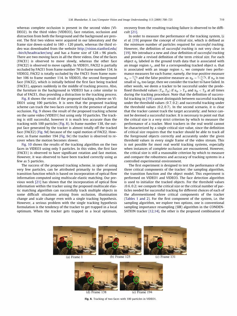
whereas complete occlusion is present in the second video (VI-DEO2). In the third video (VIDEO3), face rotation, occlusion anddistraction from both the foreground and the background are pres-ent. The first two videos were acquired in our laboratory and theframe size down-scaled to 180� 120 pixels, whereas the third vi-deo was downloaded from the website http://vision.stanford.edu/~birch/headtracker/seq/ and has a frame size of 128� 96 pixels.There are two moving faces in all the three videos. One of the faces(FACE1) is observed to move slowly, whereas the other face(FACE2) is observed to move rapidly. In VIDEO1, FACE2 is partiallyoccluded by FACE1 from frame number 78 to frame number 134. InVIDEO2, FACE2 is totally occluded by the FACE1 from frame num-ber 106 to frame number 114. In VIDEO3, the second foregroundface (FACE2), which is initially behind the first face being tracked(FACE1), appears suddenly in the middle of tracking process. Also,the furniture in the background in VIDEO3 has a color similar tothat of FACE1, thus providing a distraction to the tracking process.

Fig. 8 shows the result of the proposed tracking scheme on VI-DEO1 using 100 particles. It is seen that the proposed trackingscheme can track the two faces correctly in the presence of partialocclusion. Fig. 9 shows the result of the proposed tracking schemeon the same video (VIDEO1) but using only 10 particles. The track-ing is still successful, however it is much less accurate than thetracking with 100 particles (Fig. 8). In frame number 138, the out-put face generated by the tracker is almost totally off the trackedface (FACE2) (Fig. 9d) because of the rapid motion of FACE2. How-ever, in frame number 194 (Fig. 9e) the tracker is observed to re-cover when the motion becomes slower.

Fig. 10 shows the results of the tracking algorithm on the twofaces in VIDEO3 using only 5 particles. In this video, the first face(FACE1) is observed to have significant rotation and fast motion.However, it was observed to have been tracked correctly using asfew as 5 particles.

The success of the proposed tracking scheme, in spite of usingvery few particles, can be attributed primarily to the proposedtransition function which is based on incorporation of optical flowinformation computed using multiscale elastic matching. Our pre-vious work [21] has shown that the incorporation of optical flowinformation within the tracker using the proposed multiscale elas-tic matching algorithm can successfully track multiple objects insome difficult situations arising from occlusion, illuminationchange and scale change even with a single tracking hypothesis.However, a serious problem with the single tracking hypothesisformulation is the tendency of the tracker to get trapped in a localoptimum. When the tracker gets trapped in a local optimum,

Fig. 8. Tracking of two faces wi

recovery from the resulting tracking failure is observed to be diffi-cult [21].

In order to measure the performance of the tracking system, Liet al. [19] propose the concept of critical size, which is defined asthe minimum number of particles required for successful tracking.However, the definition of successful tracking is not very clear in[19]. We introduce a new and clear definition of successful trackingand provide a revised definition of the term critical size. For eachobject og labeled in the ground truth data that is associated withan image region rg , and for a corresponding tracked object ot thatis associated with an image region rt , we compute two perfor-mance measures for each frame; namely, the true positive measureatp ¼ rt\rg

rgand the false positive measure as afp ¼ rt�rt\rg

rg. If atp is too

small or afp too large, then we consider the tracker to have failed. Inother words, we deem a tracker to be successful under the prede-fined threshold values ðTtp; TfpÞ if atp > Ttp and afp < Tfp at all timesduring the tracking procedure. Note that the definition of success-ful tracking in [19] cannot distinguish between successful trackingunder the threshold values ð0:7;0:2Þ and successful tracking underthe threshold values ð0:2;0:7Þ. In the second scenario, it is clearthat the tracker cannot track the target accurately; and hence can-not be deemed a successful tracker. It is necessary to point out thatthe critical size is a very strict criterion by which to measure theperformance of a tracker. Most trackers in the real world cannotbe characterized by a single critical size value, since the definitionof critical size requires that the tracker should be able to track allthe foreground objects correctly and accurately under the giventhreshold values in every single frame of the video stream. Thisis not possible for most real world tracking systems, especiallywhen instances of complete occlusion are encountered. However,the critical size is still a reasonable criterion by which to measureand compare the robustness and accuracy of tracking systems in acontrolled experimental environment.

The first experiment is designed to test the performance of thethree critical components of the tracker: the sampling algorithm,the transition function and the object model. This experiment isperformed on VIDEO1 and VIDEO3. The face detection algorithmis used to initialize the tracked objects. For the threshold valuesð0:6;0:2Þwe compute the critical size or the critical number of par-ticles needed for successful tracking for different choices of each ofthe aforementioned three critical components of the tracker(Tables 1 and 2). For the first component of the system, i.e. thesampling algorithm, we explore two options, one is conventionalsampling importance resampling (SIR) algorithm in the CONDEN-SATION tracker [12,14], the other is the proposed combination of

th 100 particles in VIDEO1.

Fig. 9. Tracking of two faces with 10 particles in VIDEO1.

Fig. 10. Tracking of two faces with 5 particles in VIDEO3.

720 S.M. Bhandarkar, X. Luo / Computer Vision and Image Understanding 113 (2009) 708–725

the GA and the SIR algorithm termed as GA-CONDENSATION. Forthe second component, i.e. the transition function, we examinetwo possibilities, one is the Kalman filter [19], and the other isthe proposed transition function that incorporates optical flowinformation via multiscale elastic matching. The third componentis the object model, for which we have explored two possibilities,i.e. the region model and the region model combined with theshape model. Since there are two choices for each of the aforemen-tioned components, there are, in all, eight possible ways in whichto configure the final tracker (Tables 1 and 2).

For each of the eight distinct system configurations, we obtainthe critical size under the threshold values ð0:6;0:2Þ. We also mea-sure the tracking speed measured in terms of the number of framesprocessed per second (fps) for each of eight system configurations(Tables 1 and 2). In this experiment, we use the face detection algo-rithm only to bootstrap the tracking algorithm. It is very interest-ing to observe that all the system configurations without the

Table 1Comparison of tracking performance for different system configurations on VIDEO1.CON: CONDENSATION, KF: Kalman Filter, OF: Optical Flow, GA-CON: the CONDEN-SATION combined with GA. *The tracking speed in frames/sec is measured using 100particles.

SamplingAlgorithm

TransitionFunction

Object Model criticalsize

Frames persecond

CON KF REGION N/A 7.2*

GA-CON KF REGION N/A 7.1*

CON KF REGION andSHAPE

N/A 6.5*

GA-CON KF REGION andSHAPE

N/A 6.3*

CON OF REGION 100 6.3GA-CON OF REGION 80 7.0CON OF REGION and

SHAPE20 10.4

GA-CON OF REGION andSHAPE

12 14.2

proposed transition function (that incorporates optical flow infor-mation via multiscale elastic matching) fail when one face occludesanother. However, for the sake of measuring tracking speed, 100particles are used. This experiment shows that the transition func-tion that incorporates optical flow information via multiscaleelastic matching is very critical to the robustness, accuracy andreal-time performance of the tracking system (Tables 1 and 2).When comparing the performance of the tracker with and withoutthe proposed shape model, we observe that the incorporation ofthe shape model greatly improves the robustness of the trackingsystem measured in terms of the critical size at the cost of a verysmall reduction in tracking speed. It is also evident that the incor-poration of the GA also contributes to the improvement in the per-formance of the tracker (Tables 1 and 2) since the same trackingperformance is achieved with a smaller critical size (i.e., fewer par-ticles) resulting in a faster frame processing rate. From Tables 1and 2, one can see that similar results are obtained for VIDEO1

Table 2Comparison of tracking performance for different system configurations on VIDEO3.*The tracking speed in frames/sec is measured using 60 particles.

SamplingAlgorithm

TransitionFunction

Object Model criticalsize

Frames persecond

CON KF REGION N/A 10.4*

GA-CON KF REGION N/A 10.1*

CON KF REGION andSHAPE

N/A 9.5*

GA-CON KF REGION andSHAPE

N/A 9.3*

CON OF REGION 60 8.4GA-CON OF REGION 60 9.2CON OF REGION and

SHAPE8 16.1

GA-CON OF REGION andSHAPE

5 16.6

Fig. 11. VIDEO1: The particle distribution with and without the proposed shape model.

S.M. Bhandarkar, X. Luo / Computer Vision and Image Understanding 113 (2009) 708–725 721

and VIDEO3. The frame processing rate is higher in the case of VI-DEO3 on account of its smaller frame size. In the case of VIDEO3,the second face (FACE2) was not considered in the critical sizemeasurement since it appears very briefly in the video sequence.

In the second experiment, we compare the tracking accuracy ofthe aforementioned system configurations with and without theshape model. Fig. 11 depicts a visual comparison of the trackingaccuracy in VIDEO1 with and without the proposed shape model.Fig. 11a shows the particle distribution when the shape model isused, where the centroids of the particles are labeled with redspots. Likewise, Fig. 11b shows the particle distribution when theshape model is not used. It can be seen that when the proposedshape model is used, the particles are concentrated and closely dis-tributed around the actual locations of the faces, whereas the par-ticles are sparsely distributed when the shape model is not used.This explains why much fewer particles are needed when the pro-posed shape model is used. Fig. 12 compares the tracking accuracyin VIDEO1 of two of the eight system configurations with and with-out the proposed shape model where both system configurationsuse 100 particles. Both system configurations use the SIR algorithmwithout the incorporation of the GA and without the proposedtransition function (that incorporates optical flow information viamultiscale elastic matching). From Fig. 12, it is evident that theintroduction of the proposed shape model improves significantlythe tracking accuracy in VIDEO1. In VIDEO1, the face detection ratewas observed to be approximately 90%. The failure of face detec-tion was caused mostly by instances of partial occlusion betweenthe faces. However, the tracking algorithm was able to recoverand correctly track all the faces in all of the system configurationswhere the proposed transition function (which incorporates opti-cal flow information via multiscale elastic matching) was used.Similar results on VIDEO3 are shown in Fig. 13.

In the third experiment, we examine the performance of thetracking algorithm on VIDEO1 with and without the crossover oper-ator of the GA, as shown in Fig. 14. Both versions of the tracking algo-rithm use the object shape model and the object color model.However, the first version uses the SIR algorithm of the CONDENSA-TION-based tracker [14], whereas the second version uses the SIRalgorithm combined with the crossover operator of the GA. Both ver-sions of the tracker use 100 particles. The experimental results showthat incorporation of the crossover operator of the GA improves thetrue positive rate. In this experiment, the false positive rates are ob-served to be very similar for both versions, i.e., with and without thecrossover operator of the GA. However, the true benefit of using a GAstems from the fact that same tracking performance is achieved witha smaller critical size (Tables 1 and 2).

In the fourth experiment, we investigate a system where thetracker is integrated with the face detection algorithm. In the sec-ond video (VIDEO2), none of the tracking algorithms can correctly

track FACE2 when it is totally occluded by FACE1 (Fig. 15a). Inother words, the critical size criterion cannot be applied to com-pare the various tracking system configurations on this video. Inthe algorithm that integrates face tracking and face detection, ifthe likelihood of the second face (FACE2) is very small for a certaintime period, then it is deleted in the validation process (Fig. 15b).Fig. 16 shows the log-likelihood of the face at the point of trackingfailure. The log-likelihood value of FACE2 decreases sharply andthen returns to its normal value. The rapid decrease in the log-like-lihood value of FACE2 is caused by the failure of the tracking pro-cedure, which could be attributed to two possible reasons. The firstreason is that FACE2 moves too rapidly, in which case, the trackingalgorithm cannot keep up with the actual location of the face. Thesecond reason is that when occlusion occurs, the tracking algo-rithm cannot keep up with FACE2. However, in some cases, asshown in Fig. 16, the log-likelihood value for one of the faces doesreturn to a normal level. This could also be caused by two reasons.The first reason is that the moving face has slowed down, and thetracking algorithm is able to recover and resume correct tracking.The second reason is that when the two faces move together, theimage region corresponding to the occluded face may still have ahigh log-likelihood value, but the log-likelihood value actually cor-responds to the image region of the occluding object (FACE1) andnot the occluded object (FACE2). A simple region-based objectmodel cannot resolve this ambiguity. A higher level of occlusionreasoning based on face recognition is needed in such cases.

If a sharp decrease in the log-likelihood value of an object oc-curs when two objects move together, we remove the object fromthe tracking algorithm and using the detection algorithm to detectit when it reappears within the field of view of the camera. How-ever, the recovery of the object label is much more difficult. Thenewly detected object could be the occluded object, or could alsobe a new object. Recovery of the object label would entail usingan object (face) recognition procedure which is not within the cur-rent scope of the paper. Instead, we always assign a new label tothe newly detected object. After the object appears again, it is de-tected by the object (face) detection algorithm. A new instance ofthe object is created for each particle. It can be observed that sincethe new instance of the object is generated randomly, the corre-sponding particles are randomly distributed in the vicinity of thedetected object (Fig. 17a). However, after several iterations, thetracking algorithm is observed to rapidly converge so that the par-ticles are compactly distributed around the centroid of the newlydetected object (face) (Fig. 17b).

In the fifth experiment we show the results of a tracking algo-rithm that employs a single tracking hypothesis and incorporatesoptical flow information computed using the proposed multiscaleelastic matching algorithm. The particle filtering framework, objectregion model and object shape model are not used but occlusion

Fig. 12. VIDEO1: The tracking accuracy with and without the shape model.

Fig. 13. VIDEO3: The tracking accuracy with and without the shape model.

Fig. 14. VIDEO1: The comparison of the SIR algorithm and the SIR algorithmcombined with the GA.

722 S.M. Bhandarkar, X. Luo / Computer Vision and Image Understanding 113 (2009) 708–725

reasoning is performed [21]. Fig. 18a shows snapshots from thetracking of an eraser in a video with the camera zooming inwhereas Fig. 18b shows snapshots of the tracking of an eraser ina video with the camera zooming out. Fig. 18 shows that the pro-

posed transition function based on optical flow computation is ableto handle significant changes in the object size. Fig. 19a showssnapshots of a tracked object undergoing in-plane rotation andFig. 19b shows snapshots of a video undergoing illuminationchange. Fig. 19 shows that the proposed transition function basedon optical flow computation via multiscale elastic matching canhandle object rotation and illumination changes. The illuminationchange is well handled because of the incorporation of color gradi-ent information in the feature vector rl used in the optical flowcomputation (Eq. (12)). The imposition of inter-pixel constraintsin the optical flow computation (Eq. (12)) makes it feasible to alsohandle large changes in scale and instances of partial occlusion.Fig. 20a shows snapshots of the tracking of a face with largechanges in scale whereas Fig. 20b shows snapshots of the trackingof a face in the presence of partial occlusion. Fig. 21 shows thetracking of two faces where one face partially occludes another.These examples show that the proposed transition function basedon optical flow computation via multiscale elastic matching iscapable of handling instances of partial occlusion and also enablesocclusion reasoning [21].

It is seen that the optical flow computed using multiscale elasticmatching enables accurate estimation of the 2-D velocity field inthe image. In fact, the optical flow thus computed can be usedfor tracking in its own right. However, since only a single trackinghypothesis is maintained and no object model is used, a trackerbased on optical flow alone lacks the ability to correct localizationerrors over the course of object tracking. This causes the trackingerror to accumulate over time. It is observed that the localizationaccuracy of the contours of the tracked objects typically diminishesover time. This is particularly true in cases where there are multi-ple objects to be tracked and the tracked objects exhibit large andrapid shape deformations. This underscores the need for a goodstatistical object model and a particle filtering framework in orderto ensure robust tracking over the long term. A good statistical ob-ject model provides a validation component within the trackingsystem, which corrects the tracking errors. A particle filteringframework maintains multiple alternative tracking hypotheses atevery stage of the tracking procedure, thus enabling robust track-ing in complex multiple object scenarios. Finally, it must be notedthat the proposed system does employ tables, such as the hash ta-ble for computing the shape-based likelihood and the lookup tablefor computing the region-based likelihood, in the interest ofimproving the run-time performance. However, the overall mem-ory overhead associated with these tables was observed to be lessthan 32 MBytes which is well within the capacity of any currentdesktop or laptop computer.

10. Conclusions and future work

In this paper, a multiple object tracking framework that inte-grates object detection and object tracking was proposed. Four ma-jor improvements were made over the conventional particlefiltering-based tracking framework. These improvements were ob-served to reduce the number of particles needed for robust track-ing, thus making the proposed tracking system more robust andcomputationally more efficient. First, a novel proposal distributionand novel transition function were proposed based on the incorpo-ration of optical flow computed using multiscale elastic matching.The proposed transition function was shown to be substantiallydifferent from the existing prediction-based transition functionsused in most existing tracking systems. In prediction-based transi-tion functions, simple linear prediction models are typically used.Since linear prediction is based on historical observations andapproximation of the observed velocity by a linear model, it ismuch less accurate. The primary advantage of using the proposed

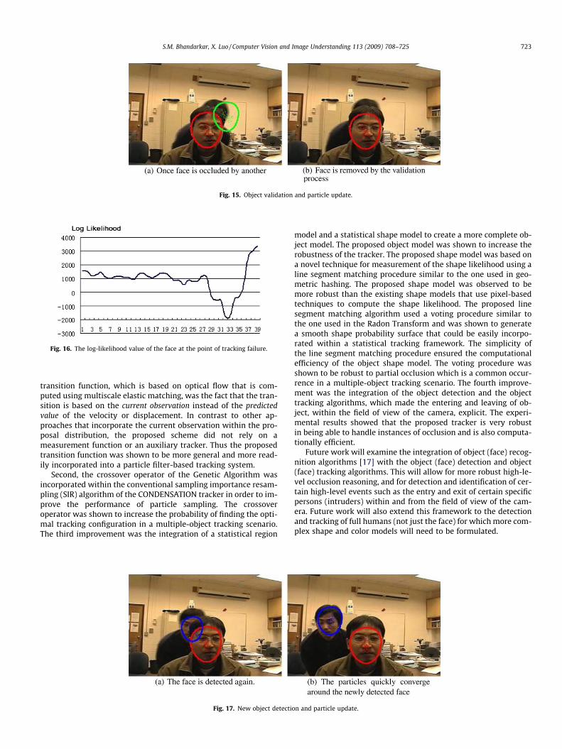
Fig. 15. Object validation and particle update.

Fig. 16. The log-likelihood value of the face at the point of tracking failure.

S.M. Bhandarkar, X. Luo / Computer Vision and Image Understanding 113 (2009) 708–725 723

transition function, which is based on optical flow that is com-puted using multiscale elastic matching, was the fact that the tran-sition is based on the current observation instead of the predictedvalue of the velocity or displacement. In contrast to other ap-proaches that incorporate the current observation within the pro-posal distribution, the proposed scheme did not rely on ameasurement function or an auxiliary tracker. Thus the proposedtransition function was shown to be more general and more read-ily incorporated into a particle filter-based tracking system.

Second, the crossover operator of the Genetic Algorithm wasincorporated within the conventional sampling importance resam-pling (SIR) algorithm of the CONDENSATION tracker in order to im-prove the performance of particle sampling. The crossoveroperator was shown to increase the probability of finding the opti-mal tracking configuration in a multiple-object tracking scenario.The third improvement was the integration of a statistical region

Fig. 17. New object detectio

model and a statistical shape model to create a more complete ob-ject model. The proposed object model was shown to increase therobustness of the tracker. The proposed shape model was based ona novel technique for measurement of the shape likelihood using aline segment matching procedure similar to the one used in geo-metric hashing. The proposed shape model was observed to bemore robust than the existing shape models that use pixel-basedtechniques to compute the shape likelihood. The proposed linesegment matching algorithm used a voting procedure similar tothe one used in the Radon Transform and was shown to generatea smooth shape probability surface that could be easily incorpo-rated within a statistical tracking framework. The simplicity ofthe line segment matching procedure ensured the computationalefficiency of the object shape model. The voting procedure wasshown to be robust to partial occlusion which is a common occur-rence in a multiple-object tracking scenario. The fourth improve-ment was the integration of the object detection and the objecttracking algorithms, which made the entering and leaving of ob-ject, within the field of view of the camera, explicit. The experi-mental results showed that the proposed tracker is very robustin being able to handle instances of occlusion and is also computa-tionally efficient.

Future work will examine the integration of object (face) recog-nition algorithms [17] with the object (face) detection and object(face) tracking algorithms. This will allow for more robust high-le-vel occlusion reasoning, and for detection and identification of cer-tain high-level events such as the entry and exit of certain specificpersons (intruders) within and from the field of view of the cam-era. Future work will also extend this framework to the detectionand tracking of full humans (not just the face) for which more com-plex shape and color models will need to be formulated.

n and particle update.

Fig. 21. Multiple face tracking using optical flow.

Fig. 19. Object tracking using optical flow with in-plane rotation and illumination change.

Fig. 20. Single face tracking using optical flow.

Fig. 18. Object tracking using optical flow with camera zoom in and zoom out.

724 S.M. Bhandarkar, X. Luo / Computer Vision and Image Understanding 113 (2009) 708–725

Appendix A. Supplementary data

Supplementary data associated with this article can be found, inthe online version, at doi:10.1016/j.cviu.2008.11.010.

References

[1] R. Bajcsy, S. Kovacic, Multiresolution elastic matching, Computer Vision,Graphics, and Image Processing 46 (1) (1989) 1–21.

[2] A. Blake, R. Curwen, A. Zisserman, A framework for spatio-temporal control inthe tracking of visual contours, International Journal of Computer Vision 11 (2)(1993) 127–145.

[3] K. Branson, S. Belongie, Tracking multiple mouse contours (without too manysamples), in: Proc. IEEE Conf. Computer Vision Pattern Recognition (CVPR), vol.1, San Diego, CA, 2005, pp. 1039–1046.

[4] J. Bouguet, Pyramidal implementation of the Lucas–Kanade feature tracker:description of the algorithm, OpenCV Documentation. Available from: http://www.intel.com/research/mrl/research/opencv/.

[5] C. Chuang, C. Kuo, Wavelet deformable model for shape description andmultiscale elastic matching, in: Proc. SPIE Symposium on VisualCommunications and Image Processing, Cambridge, MA, 1993.

[6] D. Chung, W.J. MacLean , S. Dickinson, Integrating region and boundaryinformation for improved spatial coherence in object tracking, in: Proc. IEEEConf. Computer Vision and Pattern Recognition (CVPR), Washington, DC, June2004.

[7] D. Comaniciu, V. Ramesh, P. Meer, Kernel-based object tracking, IEEETransactions on Pattern Analysis and Machine Intelligence (PAMI) 25 (5)(2003) 564–567.

[8] S.R. Deans, The Radon Transform and Some of Its Applications, John Wiley andSons, New York, NY, 1983.

[9] W. Grimson, D. Huttenlocher, On the verification of hypothesized matches inmodel-based recognition, IEEE Transactons on Pattern Recognition andMachine Intelligence (PAMI) 13 (12) (1991) 1201–1213.

[10] P. Golland, A.M. Bruckstein, Motion from Color, Center for Intelligent SystemsTR #9513, Computer Science Department, Technion, Haifa, August 1997.

[11] C. Harris, M. Stephens, A combined corner and edge detector, in: Proc. FourthAlvey Vision Conference, Manchester, UK, 1988, pp. 147–151.

[12] M. Isard, A. Blake, CONDENSATION—conditional density propagation for visualtracking, International Journal of Computer Vision (IJCV) 29 (1) (1998) 5–28.

[13] M. Isard, A. Blake, ICONDENSATION: unifying low-level and high-level trackingin a stochastic framework, Lecture Notes in Computer Science 1406 (1998)893–908.

[14] M. Isard, J. MacCormick, BraMBLe: a Bayesian multiple-blob tracker, in: Proc.Intl. Conf. Computer Vision, vol. 2, Vancouver, Canada, July 2001, pp. 34–41.

[15] M.C. Jones, Discretized and interpolated kernel density estimates, Journal ofAmerican Statistcs Association (84) (1989) 733–741.

[16] D. Koller, J.W. Weber, J. Malik, Robust multiple car tracking with occlusionreasoning, in: Proc. European Conf. Computer Vision, Stockholm, Sweden,1994, pp. 189–196.

[17] M. Lades, J. Vorbruggen, J. Buhmann, J. Lange, C.V.D. Malburg, R. Wurtz,Distortion invariant object recognition in the dynamic link architecture, IEEETransactions on Computers 42 (3) (1992) 300–311.

S.M. Bhandarkar, X. Luo / Computer Vision and Image Understanding 113 (2009) 708–725 725

[18] V. Lepetit, J. Pilet, P. Fua, Point matching as a classification problem for fast androbust object pose estimation, in: Proc. IEEE Conf. Computer Vision andPattern Recognition, vol. 2, Washington, DC, June 2004, pp. 244–250.

[19] P. Li, T. Zhang, A.E.C. Pece, Visual contour tracking based on particle filters,Image and Vision Computing 21 (2003) 111–123.

[20] B.D. Lucas, T. Kanade, An iterative image registration technique with anapplication to stereo vision, in: Proc. DARPA Image Understanding Workshop,1981, pp. 121–130.

[21] X. Luo, S.M. Bhandarkar, Tracking of multiple objects using optical flow-basedmultiscale elastic matching, in: Proc. Workshop on Dynamical Vision at theIntl. Conf. Computer Vision (ICCV), Beijing, China, October 2005, pp. 203–217.

[22] S. Malik, G. Roth, C. McDonald, Robust corner tracking for real-time augmentedreality, in:Proc. VisionInterface, Calgary, Alberta, Canada, May 2002, pp. 399–406.

[23] V. Markandey, B.E. Flinchbaugh, Multispectral constraints for optical flowcomputation, in: Proc. Intl. Conf. Computer Vision (ICCV), Osaka, Japan,December 1990, pp. 38–41.

[24] D. Martin, C. Fowlkes, J. Malik, Learning to detect natural image boundariesusing local brightness, color, and texture cues, IEEE Transactions on PatternAnalysis and Machine Intelligence 26 (5) (2004) 530–549.

[25] S.J. McKenna, S. Jabri, Z. Duric, A. Rosenfeld, H. Wechsler, Tracking groups ofpeople, Computer Vision and Image Understanding 80 (2000) 42–56.

[26] P. Meer, B. Georgescu, Edge detection with embedded confidence, IEEETransactions on Pattern Analysis and Machine Intelligence 23 (12) (2001)1351–1365.

[27] M. Mitchell, An Introduction to Genetic Algorithms, MIT Press, Cambridge, MA,1996.

[28] K. Nummiaro, E. Koller-Meier, L.V. Gool, An adaptive color-based particle filter,Image and Vision Computing 21 (1) (2003) 99–110.

[29] K. Okuma, A. Taleghani, N. De Freitas, J.J. Little, D.G. Lowe, A boosted particlefilter: multitarget detection and tracking, in: Proc. European Conf. ComputerVision (ECCV), Prague, Czech Republic, May 2004, pp. 28–39.

[30] M. Pietikainen, T. Maenpaa, J. Virtola, Color texture classification with colorhistogram and local binary patterns, in: Proc. Intl. Wkshp. Texture Analysisand Synthesis, Copenhagen, UK, June 2002, pp. 109–112.

[31] F. Porikli, A fast way to extract histograms in cartesian spaces, in: Proc. IEEEConf. Computer Vision Pattern Recognition, vol. 1., San Diego, CA, 2005, pp.829–836.

[32] W.J. Rucklidge, Locating objects using the Hausdorff distance, in: Proc. Intl.Conf. Computer Vision, Boston, MA, June 1995, pp. 457–464.

[33] F. Stein, G. Medioni, Structural indexing: efficient 3-D object recognition, IEEETransactions on Pattern Analysis and Machine Intelligence 14 (2) (1992) 125–145.

[34] J. Sullivan, A. Blake, M. Isard, J. MacCormick, Object localization by Bayesiancorrelation, in: Proc. Intl. Conf. Computer Vision, vol. 2, Corfu, Greece,September 1999, pp. 1068–1075.

[35] M. Tang, S. Ma, A fast algorithm for multiresolution elastic matching, in: Proc.10th Scandinavian Conf. Image Analysis, Lappeenranta, Finland, June 1997.

[36] D. Terzopoulos, R. Szeliski, Tracking with Kalman Snakes, in Active Vision, MITPress, Cambridge, MA, 1993. pp. 3–20.

[37] P. Toft, The Radon Transform—Theory and Implementation, Ph.D. Thesis,Department of Mathematical Modelling, Technical University of Denmark,June 1996.

[38] J. Vermaak, A. Doucet, P. Perez, Maintaining multi-modality through mixturetracking, in: Proc. Intl. Conf. Computer Vision, Nice, France, October 2003.

[39] P. Viola, M.Jones, Rapid object detection using a cascade of simple features, in:Proc. IEEE Conf. Computer Vision Pattern Recognition, Honolulu, Hawaii, June2001.

[40] P. Viola, M. Jones, Robust real-time face detection, International Journal ofComputer Vision 52 (2) (2004) 137–154.

[41] H. Wang, D. Suter, K. Schindler, Effective appearance model and similaritymeasure for particle filtering and visual tracking, in: Proc. European Conf.Computer Vision, vol. 3953, 2006, pp. 606–618

[42] H.J. Wolfson, I. Rigoutsos, Geometric hashing: an overview, IEEEComputational Science and Engineering 4 (4) (1997) 10–21.

[43] B.D. Zarit, B.J. Super, F.K.H. Quek, Comparison of five color models in skinpixel classification, in: Intl. Wkshp. Recognition, Analysis, and Tracking ofFaces and Gestures in Real-Time Systems, Washington, DC, September 1999,pp. 58–63.