1

GEOPHYSICAL APPLICATIONS

M. D. Prouty, I. Hrvoic, A. Vershovski

1 .1 A i rbo rne magnetometers and g rad io meters Along with electromagnetic (EM), gravity, and radiation detection methods, magnetometry is a basic method for geophysical exploration for minerals, including diamonds, and oil. Fixed-wing and helicopter-borne magnetometers and gradiometers are generally used for assessment explorations, with ground and marine methods providing for follow-up mapping of interesting areas.

Magnetometers have been towed by or mounted on airborne platforms for resource exploration since the 1940s [18]. Mapping of the Earths magnetic field can illuminate structural geology relating to rock contacts, intrusive bodies, basins, and bedrock. Susceptibility contrasts associated with diering amounts of magnetite in the subsurface can identify areas that are good candidates for base and precious metal mineral deposits or diamond pipes. Existing magnetic anomalies associated with known mineralization are often extrapolated to extend drilling patterns and mining activities into new areas.

After World War I Iuxgate sensors, originally employed for submarine detection, replaced dipping needle and induction coil magneticeld d sensing systems as the airborne magnetometer of choice. While theuxgate e and induction magnetometer could measure the components of the Earthseld

d rapidly (100 Hz or more), their sensitivity to orientation made them a poor choice for installation on moving platforms. Experiments by Packard and Varian in 1953 on nuclear magnetic resonance resulted in the invention of the orientation-independent total-eld proton precession magnetometer and total-eld magnetometers replaced vector magnetometer systems in mobile platforms.

Basic research on the cesium atomic clock during the 1960s resulted in the

2 P r ou t y

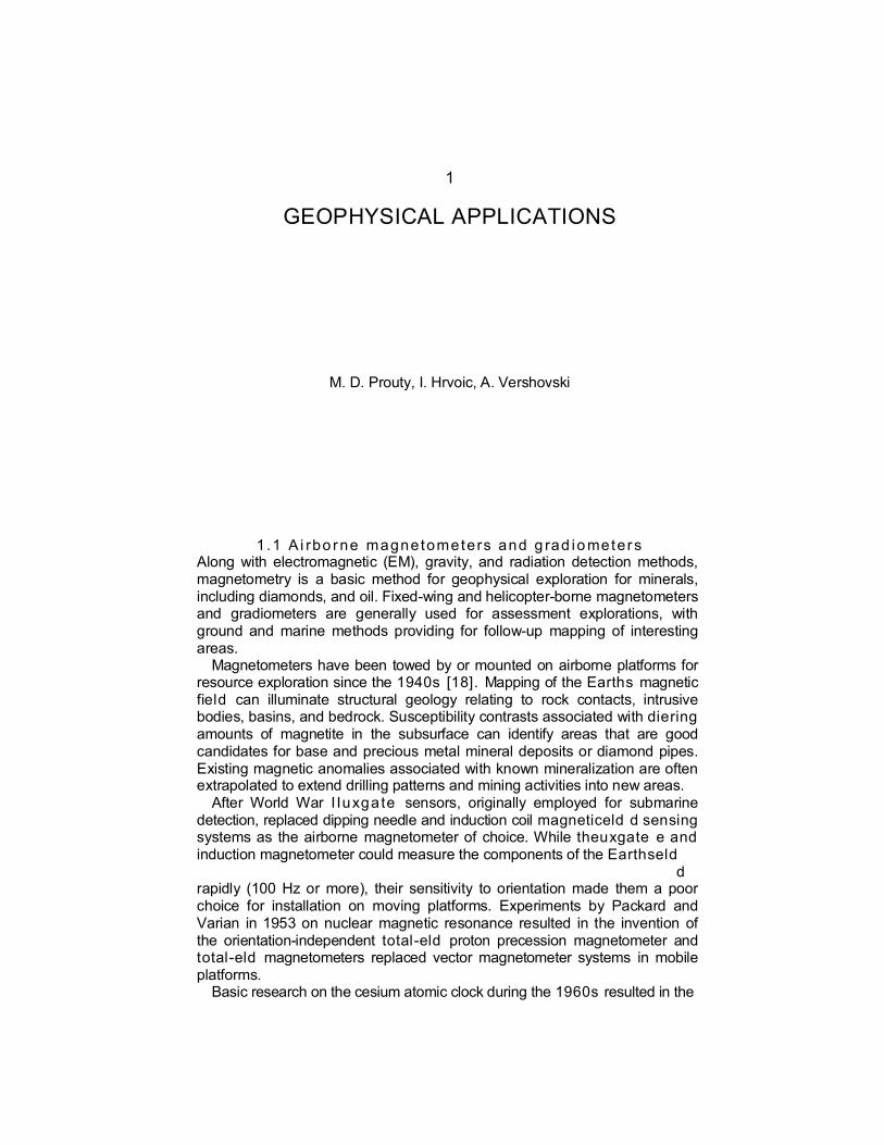
Figure 1.1 Various airborne magnetometers. Photo a) shows a helicopter-towed bird sensor. Photo b) shows a sensor mounted on a nose stinger on a helicopter. Photo c) shows a tail stinger mounted sensor. Photo d) shows a gradiometer bird for helicopter surveys.

development of high performance magnetometers with much higher sample rates and sensitivities than those using proton precession methods. These optically-pumped magnetometers replaced proton precession systems in the 1970s and 1980s. Since that time most airborne surveys have been con-ducted with high speed, high sensitivity cesium vapor or potassium magne-tometers.

The primary purpose of an airborne magnetic survey is to delineate mag-netic features of a survey area in an economical manner. Installation of one to four sensors allows for up to three gradient measurements (alongand across-track and vertical). Airborne magnetometers can be installed in wing-tip or tail-stinger housings, externally mounted inbooms, s," or towed in streamlinedbirds. " Up to 100 readings per second are utilized forxed-wing installations, providing enough sampling to allow for anti-alias pre-ltering

g of the data. Figure 1.1 shows several examples of airborne systems.

Measurements along-track cover the terrain adequately with one reading every 10 to 30 meters at a y i n g altitude of 30 to 50 meters. However, across-track measurements, determined by line spacing, are generally under-sampled and subject to the aliasing of geologic information. Aliasing can be reduced by the installation of one magnetometer on each wing tip to obtain smaller line spacing or to measure an across-track gradient.

Fixed-wing aircraft allow for high survey speeds and, therefore, faster cov-erage of desired areas. Sensors are typically mounted in nose or tail stingers and wing-tip housings to minimize interference wi th igh t t dynamics and

Geophysical applications 3

pilot practices. However, sensors mounted close to the airframe are greatly inuenced by the magnetic signature of the aircraft itself. The proximity of the conductive aircraft structure, engines, and magnetic components for control of the aircraft, along with electrical currents from the avionics, requires data compensation either in real time or in post processing. Through compensation, the signals created by the aircraft itself may be reduced by a factor or 20 or more.

Compensation systems must also subtract the complicated induced and permanent magneticelds of the aircraft and eddy currents associated with motion or acceleration of the conducting aircraft skin in the Ear thseld.

. Final data noise levels of 100 p T / H z RMS are common, and may approach 1pT using high-sensitivity vapor magnetometers, magnetically clean aircraft, and modern compensation solutions.

Signal from the airframe may be much reduced, and compensation may be entirely avoided, by mounting the magnetometers in towed birds. Towed birds are dicult to utilize in axed-wing aircraft, but are often used from helicopters. The highest quality geophysical data can often be obtained from sensors mounted in helicopter-towed birds. Direct installations on helicopter skids or stingers are rare in mineral exploration but are used for ordnance detection.

A typical helicopter installation utilizes a bird towed 100 ft or more below and behind the helicopter. Due to reduced interference from the aircraft, sys-tem sensitivities are superior, reaching 10pT or lower total-eld d noise level and few pT/m gradient sensitivities at 10 readings per second. While there is no need for active compensation in helicopter installations, higher operational costs of rotary wing aircraft make helicopter magnetometer surveys most suitable for mountainous or rough terrain or detailed surveys.

1 .2 Gro u n d magnetome te rs /grad iometers

Portable magnetometers are used for ground follow-up of airborne surveys for minerals, diamonds, and hydrocarbon structures, as well as to aid in-terpretation of seismic and electromagnetic surveys. They are also used for detection and characterization of unexploded ordnance (UXO), utilities (un-derground storage tanks, pipelines, telecommunication cables) and for rapid non-intrusive survey of archaeological sites. Alkali magnetometers are also suitable for forensic science investigations, since most excavations, such as grave sites, create a magnetic anomaly.

Single-axisuxgate magnetometers were used in ground magnetic sur-

4 Prouty

veys until the invention of the proton precession magnetometer in the late 60s. In the early 70s proton precession magnetometers became small and light weight enough to be carried as portable systems. The total-eld d mea-surement of those sensors eliminated the orientation dependence ofuxgate

e magnetometers, which measure a single component of the vectoreld.

. Proton precession magnetometers have a sample interval of approximately

0.5 to 3 seconds and require substantial power to polarize the proton-rich hydrocarbonuid prior to relaxation. Incorporating auid with a small amount of unpaired electrons and utilizing RF pumping resulted in the dynamic polarization, or Overhauser, magnetometer which requires much less power and provides faster sampling of as little as 0.2 seconds. Still, performance is limited due to the protons low frequency precession signal and the requirement of a deection pulse, which interrupts theeld-reading process.

Self-oscillating optically pumped Cesium Vapor magnetometers became available in the 80s and 90s and provided a much higher Larmor frequency and virtually continuous readings. Cesium or potassium magnetometers used in portable instruments typically sample at 10 Hz. Optically pumped magne-tometers also have improved tolerance of undesirable environmental condi-tions such as gradients and high-frequency or large-amplitude interferences.

Today, ground magnetic surveys are usually performed by making a dier-ential measurement between a roving magnetometer and a stationary base station. This technique eliminates the temporal variations of the magnetic field, which are about 10 - 30nT in amplitude over the course of a day. For good performance, base station readings must be synchronous with the roving magnetometer readings. A variety of sensor congurations s are used, including a single sensor, vertical or horizontal across track gradiometers, or multisensor arrays on carts, ski-doos or other vehicles.

Measurement of position is generally done by GPS (Global Positioning Systems). Previous methods of cutting survey lines and marking measure-ment points withags are now largely abandoned.

Ground surveys face a number of diculties, some of which do not exist in airborne installations. Magnetic contamination from the electronics and operator may result in signicant heading errors, power lines and other man-made magneticelds create interfering signals, and the presence of high gradients places greater requirements on the positioning of the sensors.

The advantages of optically pumped magnetometers greatly enhance the utility of magnetic gradient surveys, which are more susceptible to all the problems mentioned. Gradiometric measurements are helpful in more pre-cisely determining target depth and shape. Gradient maps dene e the position and shape of anomalies more sharply than magnetic maps. In addition,

Geophys ical appl icat ions 5

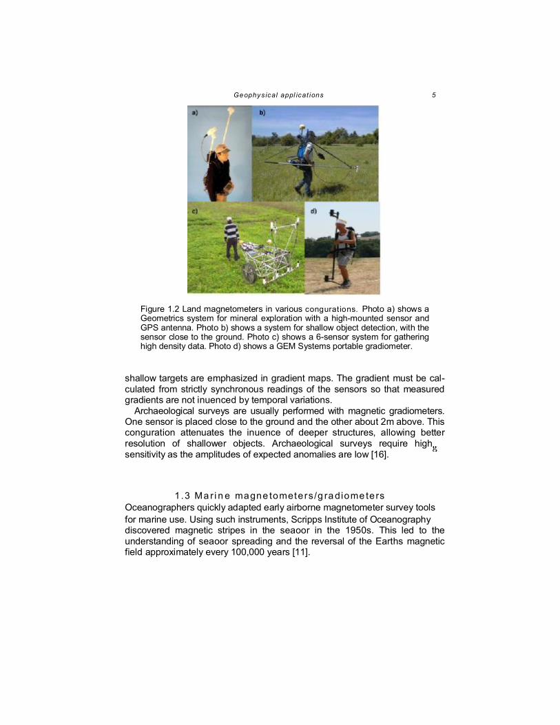
Figure 1.2 Land magnetometers in various congurations. Photo a) shows a Geometrics system for mineral exploration with a high-mounted sensor and GPS antenna. Photo b) shows a system for shallow object detection, with the sensor close to the ground. Photo c) shows a 6-sensor system for gathering high density data. Photo d) shows a GEM Systems portable gradiometer.

shallow targets are emphasized in gradient maps. The gradient must be cal-culated from strictly synchronous readings of the sensors so that measured gradients are not inuenced by temporal variations.

Archaeological surveys are usually performed with magnetic gradiometers. One sensor is placed close to the ground and the other about 2m above. This conguration attenuates the inuence of deeper structures, allowing better resolution of shallower objects. Archaeological surveys require high sensitivity as the amplitudes of expected anomalies are low [16].

1 .3 Ma r i n e magne tometers/g ra diome ters Oceanographers quickly adapted early airborne magnetometer survey tools for marine use. Using such instruments, Scripps Institute of Oceanography discovered magnetic stripes in the seaoor in the 1950s. This led to the understanding of seaoor spreading and the reversal of the Earths magnetic field approximately every 100,000 years [11].

6 Prouty

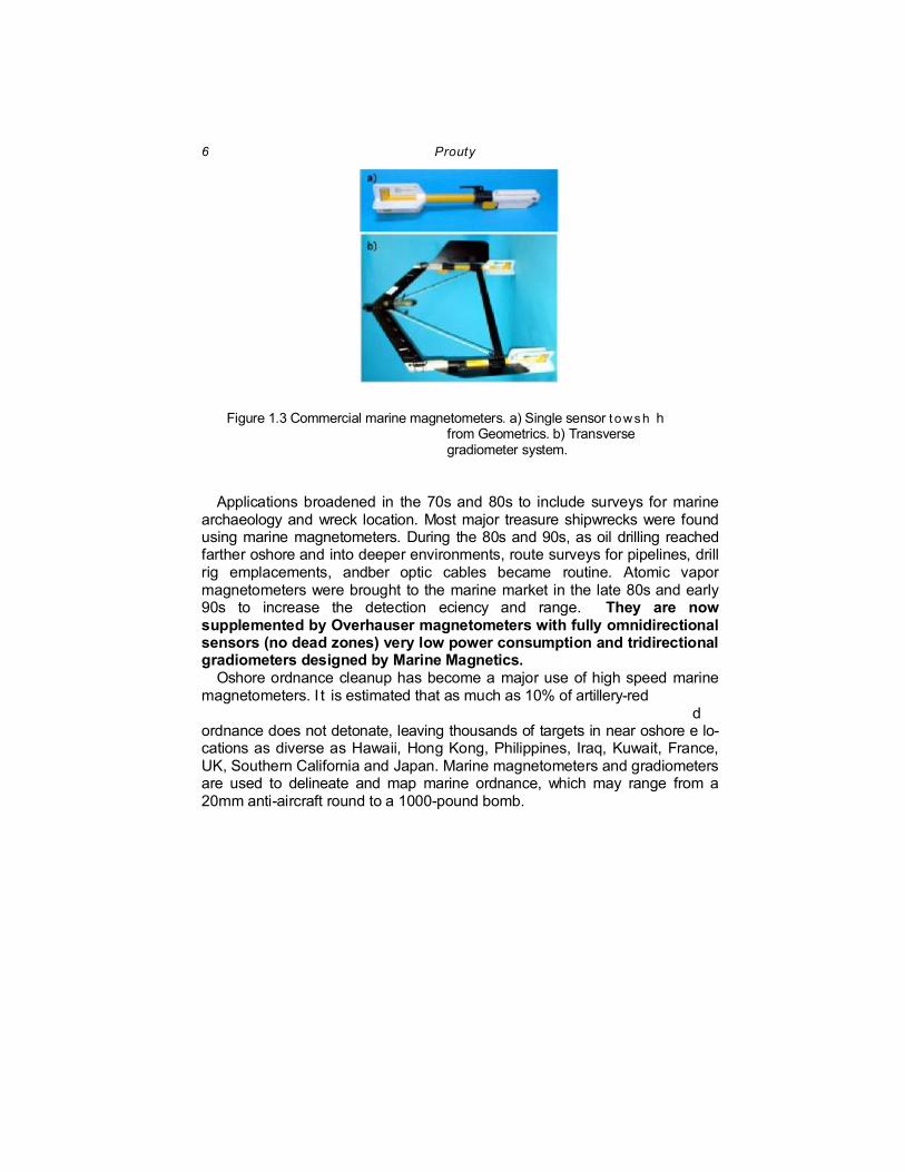
Figure 1.3 Commercial marine magnetometers. a) Single sensor t owsh h from Geometrics. b) Transverse gradiometer system.

Applications broadened in the 70s and 80s to include surveys for marine archaeology and wreck location. Most major treasure shipwrecks were found using marine magnetometers. During the 80s and 90s, as oil drilling reached farther oshore and into deeper environments, route surveys for pipelines, drill rig emplacements, andber optic cables became routine. Atomic vapor magnetometers were brought to the marine market in the late 80s and early 90s to increase the detection eciency and range. They are now supplemented by Overhauser magnetometers with fully omnidirectional sensors (no dead zones) very low power consumption and tridirectional gradiometers designed by Marine Magnetics.

Oshore ordnance cleanup has become a major use of high speed marine magnetometers. I t is estimated that as much as 10% of artillery-red

d ordnance does not detonate, leaving thousands of targets in near oshore e lo-cations as diverse as Hawaii, Hong Kong, Philippines, Iraq, Kuwait, France, UK, Southern California and Japan. Marine magnetometers and gradiometers are used to delineate and map marine ordnance, which may range from a 20mm anti-aircraft round to a 1000-pound bomb.

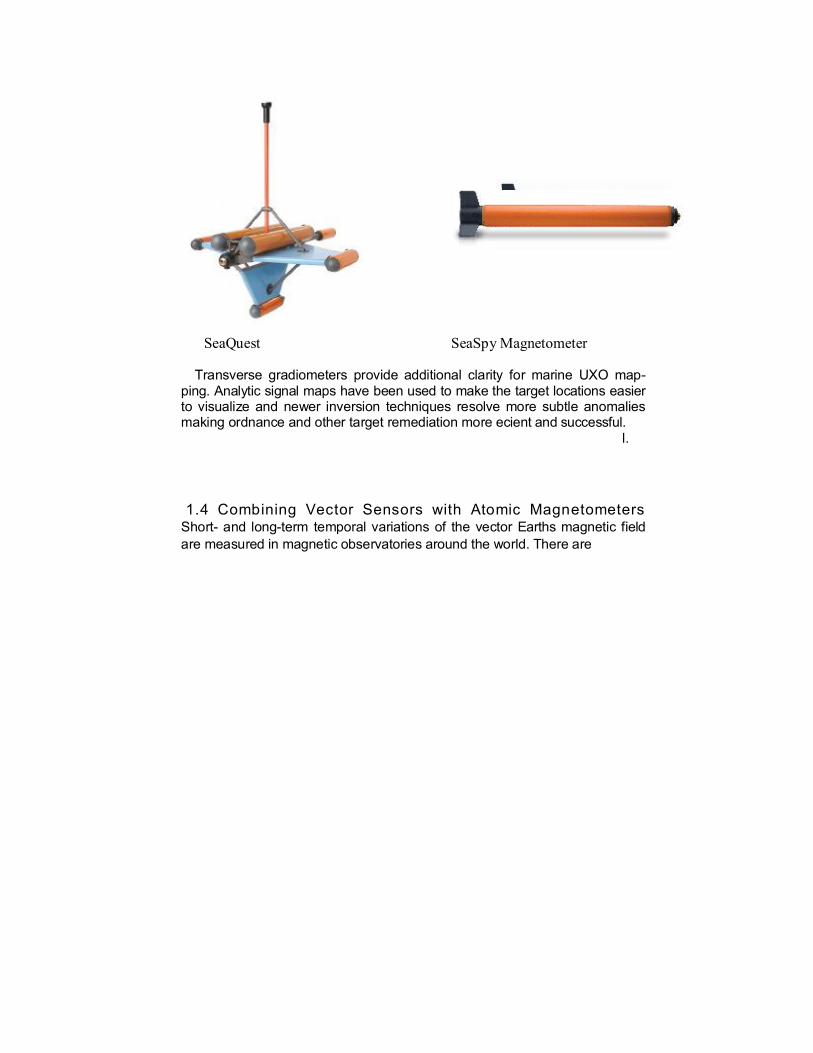
SeaQuest SeaSpy Magnetometer

Transverse gradiometers provide additional clarity for marine UXO map-ping. Analytic signal maps have been used to make the target locations easier to visualize and newer inversion techniques resolve more subtle anomalies making ordnance and other target remediation more ecient and successful.

l.

1.4 Combining Vector Sensors with Atomic Magnetometers Short- and long-term temporal variations of the vector Earths magnetic field are measured in magnetic observatories around the world. There are

8

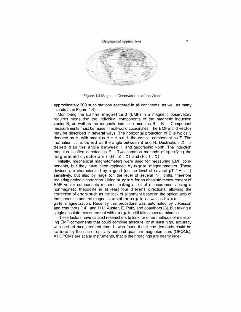
Figure 1.4 Magnetic Observatories of the World

approximately 200 such stations scattered in all continents, as well as many islands (see Figure 1.4).

Monitoring the Earths magneticeld (EMF) in a magnetic observatory requires measuring the individual components of the magnetic induction vector B, as well as the magnetic induction modulus B = B . Component measurements must be made in real-world coordinates. The EMFeld d vector may be described in several ways. The horizontal projection of B is typically denoted as H, with modulus H = H a n d the vertical component as Z. The inclination, I , is dened as the angle between B and H. Declination, D , is dened d as the angle between H and geographic North. The induction modulus is often denoted as F . Two common methods of specifying the magneticeld d vector are ( (H , Z , D ) and (F , I , D ) .

Initially, mechanical magnetometers were used for measuring EMF com-ponents, but they have been replaced byuxgate magnetometers. These devices are characterized by a good (on the level of several pT / H z ) sensitivity, but also by large (on the level of several nT) drifts, therefore requiring periodic correction. Using auxgate for an absolute measurement of EMF vector components requires making a set of measurements using a nonmagnetic theodolite in at least four dierent directions, allowing the correction of errors such as the lack of alignment between the optical axis of the theodolite and the magnetic axis of theuxgate as well as th eu x - gate magnetization. Recently this procedure was automated by J.Rasson and coauthors [14], and H.U. Auster, E. Pulz, and coauthors [3], but taking a single absolute measurement with auxgate still takes several minutes.

These factors have caused researchers to look for other methods of measur-ing EMF components that could combine absolute, or at least high, accuracy with a short measurement time. I t was found that these demands could be satised by the use of optically pumped quantum magnetometers (OPQMs). All OPQMs are scalar instruments, that is their readings are nearly inde-

9

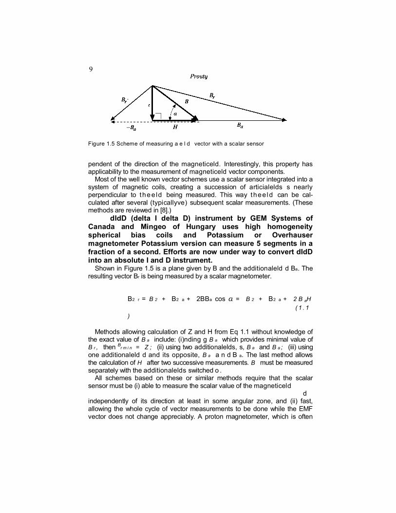
Figure 1.5 Scheme of measuring a e l d vector with a scalar sensor

pendent of the direction of the magneticeld. Interestingly, this property has applicability to the measurement of magneticeld vector components.

Most of the well known vector schemes use a scalar sensor integrated into a system of magnetic coils, creating a succession of articialelds s nearly perpendicular to the e ld being measured. This way thee ld can be cal-culated after several (typicallyve) subsequent scalar measurements. (These methods are reviewed in [8].) dIdD (delta I delta D) instrument by GEM Systems of Canada and Mingeo of Hungary uses high homogeneity spherical bias coils and Potassium or Overhauser magnetometer Potassium version can measure 5 segments in a fraction of a second. Efforts are now under way to convert dIdD into an absolute I and D instrument.

Shown in Figure 1.5 is a plane given by B and the additionaleld d Ba. The resulting vector Br is being measured by a scalar magnetometer.

B2 r = B 2 + B2 a + 2BBa cos a = B 2 + B2 a + 2 B aH ( 1 . 1)

Methods allowing calculation of Z and H from Eq 1.1 without knowledge of

the exact value of B a include: (i)nding g B a which provides minimal value of B r , then B

r m i n = Z ; (ii) using two additionalelds, s, B a and B a ; (iii) using one additionaleld d and its opposite, B a a n d B a. The last method allows the calculation of H after two successive measurements. B must be measured separately with the additionalelds switched o .

All schemes based on these or similar methods require that the scalar sensor must be (i) able to measure the scalar value of the magneticeld

d independently of its direction at least in some angular zone, and (ii) fast, allowing the whole cycle of vector measurements to be done while the EMF vector does not change appreciably. A proton magnetometer, which is often

10 used in schemes of this kind, satises therst condition, but fails to satisfy the second. Overhauser magnetometers are somewhat faster, with a rate of 5 readings/sec allowing for the cycle to be completed in 1 sec. Potassium magnetometers allow for about 0.25sec cycles. Their very low heading error assures good accuracy of measurement.

Because of their fast response, OPQMs (see Chapter 3), with their typical bandwidth of several kHz, are much better suited for use in these schemes. Th e rs t OPQM-based component device of this kind, designed by J.R. Rasson, was based on an Mz-sensor [13]. Its working cycle consisted ofve

e

Geophysical applications 11

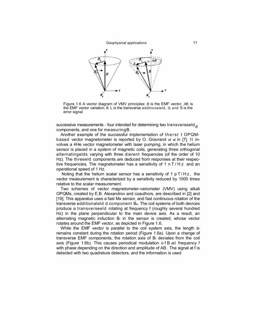
Figure 1.6 A vector diagram of VMV principles: B is the EMF vector, AB is the EMF vector variation, B L is the transverse addit ionale ld, d, and S is the error signal

successive measurements - four intended for determining two transverseeld components, and one for measuringB.

Another example of the successful implementation of the rst t OPQM-based vector magnetometer is reported by O. Gravrand et al in [7]. I t in-volves a 4He vector magnetometer with laser pumping, in which the helium sensor is placed in a system of magnetic coils, generating three orthogonal alternatingelds varying with three dierent frequencies (of the order of 10 Hz). The threeeld components are deduced from responses at their respec-tive frequencies. The magnetometer has a sensitivity of 1 n T / H z and an operational speed of 1 Hz.

Noting that the helium scalar sensor has a sensitivity of 1 p T / H z , the vector measurement is characterized by a sensitivity reduced by 1000 times relative to the scalar measurement.

Two schemes of vector magnetometer-variometer (VMV) using alkali OPQMs, created by E.B. Alexandrov and coauthors, are described in [2] and [19]. This apparatus uses a fast Mx sensor, and fast continuous rotation of the transverse additionaleld d component Ba. The coil systems of both devices produce a transverseeld rotating at frequency f (roughly several hundred Hz) in the plane perpendicular to the main device axis. As a result, an alternating magnetic induction Br in the sensor is created, whose vector rotates around the EMF vector, as depicted in Figure 1.6.

While the EMF vector is parallel to the coil system axis, the length Br remains constant during the rotation period (Figure 1.6a). Upon a change of transverse EMF components, the rotation axis of Br deviates from the coil axis (Figure 1.6b). This causes periodical modulation o f B rat frequency f with phase depending on the direction and amplitude of AB. The signal at f is detected with two quadrature detectors, and the information is used

10 Prouty

to induceelds, fully compensating for AB . The magnitude of currents in the coils generating theseelds is regarded as a measure of the transverse components of the magneticeld d B.

The signal amplitude can be estimated as being S = k B, where k = B (B2 +B2 )12. This means that the vector sensitivity of the device grows with the amplitude of the rotatingeld; unfortunately, this amplitude is limited by the stability and sensitivity of measuring the z-component of the eld B on one hand and by the scalar sensor time response on the other.

Fast Mx-sensors allow a relatively large amplitude of B , ensuring k on the level of 1/10. The variant of the VMV described in [2] uses additional 90-95% compensation of the EMF, which permits an increase in the sensitivity of measuring the transverseeld components almost by an order of magnitude (k Pz 1 16). This instrument is characterized by a sensitivity of about 0.015 nT rms at a 0.1 s sample rate, and reproducibility of the z-channel at a level of 0.15 nT.

The instruments described above are classied as variometers because their readings are not absolute: theeld they measure is inuenced by the magnetic coils. The method for the absolute measurement of magneticeld

d components, widely used in magnetic observatories, consists of zeroing two field components and measuring the third with the help of a scalar sensor. I t does not require high nullication accuracy because the contribution of small residual transverse components to theeld modulus is suppressed by a few orders of magnitude.

A scheme implying fast Cs Mx-OPQM together with relatively fast (5 Hz) switching of additionalelds was reported in [12]. The measurement cycle consists o f v e stages, ensuring an accuracy of 0.1 nT and a cycle time of 1 s. For further accuracy a slow correction of the readings of the Cs sensor may be done with a Cs-He magnetometer (see Chapter 3).

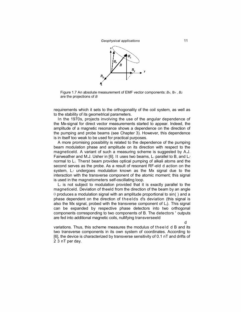
A way to measure the three components of the EMF vector with high absolute accuracy using OPQM integrated into a symmetric coil system was proposed by A.K. Vershovskiy in [19]. In this method, the compensating fields are harmonically modulated so that the resultant magneticeld vector Br in the sensor rotates, with constant magnitude, around the initial field direction, and passes in each rotation cycle through the three positions shown in Figure 1.7. At each position, two components of the magneticeld

d B are compensated with high accuracy, while the third one is fully uncom-pensated and amenable to measurement. I t has been shown theoretically that this method provides an absolute accuracy of 0.1 nT with 0.1 s time response. The main drawback of this method is related to the very strict

Geophysical applications 11

Figure 1.7 An absolute measurement of EMF vector components: BX, BY , BZ are the projections of B

requirements which it sets to the orthogonality of the coil system, as well as to the stability of its geometrical parameters.

In the 1970s, projects involving the use of the angular dependence of the Mx-signal for direct vector measurements started to appear. Indeed, the amplitude of a magnetic resonance shows a dependence on the direction of the pumping and probe beams (see Chapter 3). However, this dependence is in itself too weak to be used for practical purposes.

A more promising possibility is related to the dependence of the pumping beam modulation phase and amplitude on its direction with respect to the magneticeld. A variant of such a measuring scheme is suggested by A.J. Fairweather and M.J. Usher in [6]. I t uses two beams, Li parallel to B, and L2 normal to Li. Therst beam provides optical pumping of alkali atoms and the second serves as the probe. As a result of resonant RF-eld d action on the system, L2 undergoes modulation known as the Mx signal due to the interaction with the transverse component of the atomic moment; this signal is used in the magnetometers self-oscillating loop.

Li is not subject to modulation provided that it is exactly parallel to the magneticeld. Deviation of theeld from the direction of the beam by an angle 0 produces a modulation signal with an amplitude proportional to sin( ) and a phase dependent on the direction of the elds d's deviation (this signal is also the Mx signal, probed with the transverse component of L l). This signal can be expanded by respective phase detectors into two orthogonal components corresponding to two components of B. The detectors ' outputs are fed into additional magnetic coils, nullifying transverseeld

d variations. Thus, this scheme measures the modulus of thee ld d B and its two transverse components in its own system of coordinates. According to [6], the device is characterized by transverse sensitivity of 0.1 nT and drifts of 2 3 nT per day.

12 Prouty

The disadvantages of this scheme are common to nearly all devices employ-ing systems of additional articial magneticelds; they are 1) the presence of additional magneticelds inuencing the process of absolute measurements, and 2) absence of easy means to dene the coordinate system of the device relative to the geophysical coordinate system.

A signicant modication of the Fairweather-Usher scheme was proposed by A.K. Vershovskiy in [20]. This scheme does not stipulate using any addi-tional magneticelds and, therefore, is capable of an absolute measurement of the magneticeld vector components. Instead of the forced return of the measured magneticeld d vector B towards direction z, it is suggested to vary the direction of laser beam L1 so that it would follow the vector of the measured magneticeld. This would make it possible to relate the measure-ment to the Earths coordinate system by merely measuring the L1 beam direction, which can be done with extremely high precision.

Preliminary calculations show that this scheme can ensure the measure-ment of the modu lus,B , with an absolute accuracy of 0.02 nT, and of two angles of deviation of B with an absolute accuracy and sensitivity of no worse than 0.1 nT for a measurement time of 1 s. The accuracy of this scheme does not depend on the precision of its positioning in space. Its additional advantage is the absence of generated magneticelds, s, which makes possible its use in magnetometric observatories jointly with other devices.

Most of the instruments described in this section exist only as laboratory prototypes, whereas almost all vector measurements worldwide are being done withuxgates or proton-based magnetometers. Nevertheless, OPQMs have proven their advantages in this realm, so one can expect that commercial devices of this sort will appear.

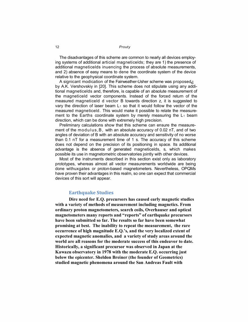
Earthquake Studies Dire need for E.Q. precursors has caused early magnetic studies

with a variety of methods of measurement including magnetics. From ordinary proton magnetometers, search coils, Overhauser and optical magnetometers many reports and “reports” of earthquake precursors have been submitted so far. The results so far have been somewhat promising at best. The inability to repeat the measurement, the rare occurrence of high magnitude E.Q.’s, and the very localized extent of expected magnetic anomalies, and a variety of study areas around the world are all reasons for the moderate success of this endeavor to date. Historically, a significant precursor was observed in Japan at the Kawazu observatory in 1978 with the moderate E.Q. occurring just below the epicenter. Sheldon Breiner (the founder of Geometrics) studied magnetic phenomena around the San Andreas Fault with

Geophysical applications 11 Rubidium optical magnetometers in 1967. (Breiner 1967) He showed several anomalies, precursors preceding the San Andreas Fault creep by tens of hours and then preceding the local earthquakes by several days. However he denies consistent correlation of magnetic signals and earthquakes. The Loma Prieta E.Q. near San Francisco in 1989 (Frazer-Smith et all 1990) produced a larger precursor (later disputed by a number of magneticins and seismologists, sometimes with somewhat unconvincing arguments). Strictly, magnetic precursors, if they exist, will have some limitations:

a) As we expect dipolar type of anomaly, the precursors will be very localized (dipolar field falls off with third potential of distance)

b) Detectable signals must be of a very low frequency as the hypocenters are deep in the earth and with even a low conductivity of the ground above, a skin effect will add severe attenuation of higher frequencies and prevent their detectability. Millihertz frequencies seem to be the upper limit.

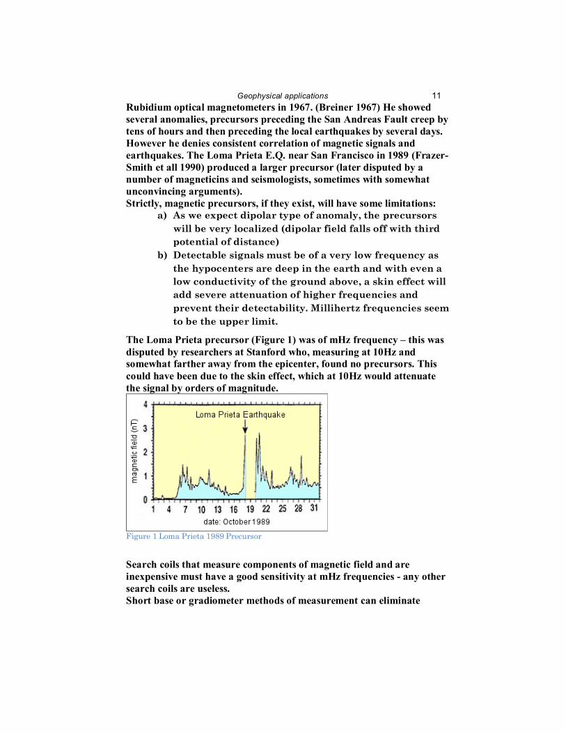
The Loma Prieta precursor (Figure 1) was of mHz frequency – this was disputed by researchers at Stanford who, measuring at 10Hz and somewhat farther away from the epicenter, found no precursors. This could have been due to the skin effect, which at 10Hz would attenuate the signal by orders of magnitude.

Figure 1 Loma Prieta 1989 Precursor

Search coils that measure components of magnetic field and are inexpensive must have a good sensitivity at mHz frequencies - any other search coils are useless. Short base or gradiometer methods of measurement can eliminate

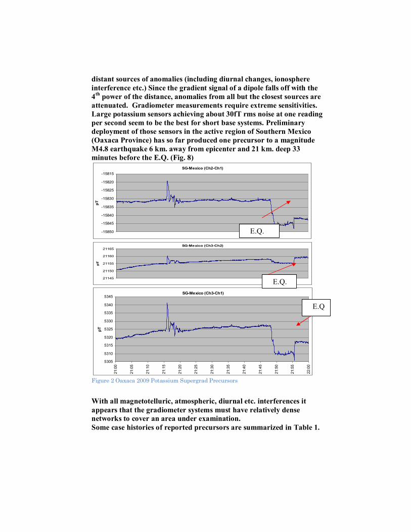
distant sources of anomalies (including diurnal changes, ionosphere interference etc.) Since the gradient signal of a dipole falls off with the 4th power of the distance, anomalies from all but the closest sources are attenuated. Gradiometer measurements require extreme sensitivities. Large potassium sensors achieving about 30fT rms noise at one reading per second seem to be the best for short base systems. Preliminary deployment of those sensors in the active region of Southern Mexico (Oaxaca Province) has so far produced one precursor to a magnitude M4.8 earthquake 6 km. away from epicenter and 21 km. deep 33 minutes before the E.Q. (Fig. 8)

SG-Mexico (Ch2-Ch1)

-15850

-15845

-15840

-15835

-15830

-15825

-15820

-15815

pT

SG-Mexico (Ch3-Ch2)

21145

21150

21155

21160

21165

pT

SG-Mexico (Ch3-Ch1)

5305

5310

5315

5320

5325

5330

5335

5340

5345

21:0

0

21:0

5

21:1

0

21:1

5

21:2

0

21:2

5

21:3

0

21:3

5

21:4

0

21:4

5

21:5

0

21:5

5

22:0

0

pT

Figure 2 Oaxaca 2009 Potassium Supergrad Precursors

With all magnetotelluric, atmospheric, diurnal etc. interferences it appears that the gradiometer systems must have relatively dense networks to cover an area under examination. Some case histories of reported precursors are summarized in Table 1.

E.Q.

E.Q.

E.Q

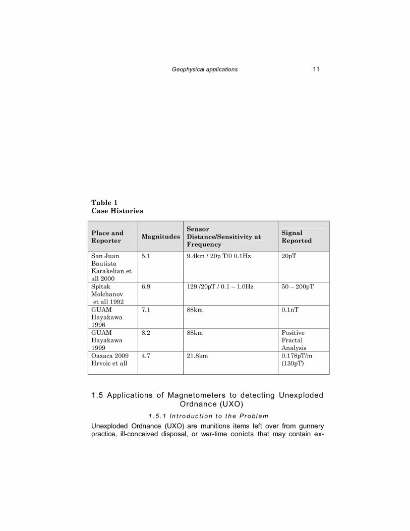
Geophysical applications 11 Table 1 Case Histories

1.5 Applications of Magnetometers to detecting Unexploded

Ordnance (UXO) 1 . 5 . 1 In t ro duc t i on t o t h e Pr obl em

Unexploded Ordnance (UXO) are munitions items left over from gunnery practice, ill-conceived disposal, or war-time conicts that may contain ex-

Place and Reporter

Magnitudes Sensor Distance/Sensitivity at Frequency

Signal Reported

San Juan Bautista Karakelian et all 2000

5.1 9.4km / 20p T/0 0.1Hz 20pT

Spitak Molchanov et all 1992

6.9 129 /20pT / 0.1 – 1.0Hz 50 – 200pT

GUAM Hayakawa 1996

7.1 88km 0.1nT

GUAM Hayakawa 1999

8.2 88km Positive Fractal Analysis

Oaxaca 2009 Hrvoic et all

4.7 21.8km 0.178pT/m (130pT)

plosive materials posing a hazard if disturbed. Items may range in size from 37mm shells to 1000-pound bombs.

Detecting UXO is distinctly easier than detecting land mines. UXO were never intended to be dicult to detect, nor to be triggered by weak vibration or low pressure contact. Thus, the detection of UXO items is considerably easier and safer than detecting land mines. UXO usually contains signicant

t

Geophysical applications 13

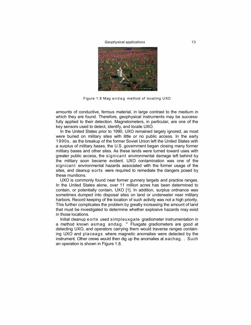
Figure 1.8 Mag a n d a g method of locat ing UXO

amounts of conductive, ferrous material, in large contrast to the medium in which they are found. Therefore, geophysical instruments may be success-fully applied to their detection. Magnetometers, in particular, are one of the key sensors used to detect, identify, and locate UXO.

In the United States prior to 1990, UXO remained largely ignored, as most were buried on military sites with little or no public access. In the early 1990s, as the breakup of the former Soviet Union left the United States with a surplus of military bases, the U.S. government began closing many former military bases and other sites. As these lands were turned toward uses with greater public access, the signicant environmental damage left behind by the military soon became evident. UXO contamination was one of the signicant environmental hazards associated with the former usage of the sites, and cleanup eorts were required to remediate the dangers posed by these munitions.

UXO is commonly found near former gunnery targets and practice ranges. In the United States alone, over 11 million acres has been determined to contain, or potentially contain, UXO [1]. In addition, surplus ordnance was sometimes dumped into disposal sites on land or underwater near military harbors. Record keeping of the location of such activity was not a high priority. This further complicates the problem by greatly increasing the amount of land that must be investigated to determine whether explosive hazards may exist in those locations.

Initial cleanup eorts used s impleuxgate gradiometer instrumentation in a method known asmag andag. " Fluxgate gradiometers are good at detecting UXO, and operators carrying them would traverse ranges contain-ing UXO and placeags where magnetic anomalies were detected by the instrument. Other crews would then dig up the anomalies at eachag. . Such an operation is shown in Figure 1.8.

14 Prouty

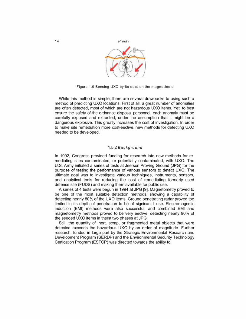
Figure 1.9 Sensing UXO by its eect on the magnet ice ld

While this method is simple, there are several drawbacks to using such a method of predicting UXO locations. First of all, a great number of anomalies are often detected, most of which are not hazardous UXO items. Yet, to best ensure the safety of the ordnance disposal personnel, each anomaly must be carefully exposed and extracted, under the assumption that it might be a dangerous explosive. This greatly increases the cost of investigation. In order to make site remediation more cost-eective, new methods for detecting UXO needed to be developed.

1.5.2 Bac kground

In 1992, Congress provided funding for research into new methods for re-mediating sites contaminated, or potentially contaminated, with UXO. The U.S. Army initiated a series of tests at Jeerson Proving Ground (JPG) for the purpose of testing the performance of various sensors to detect UXO. The ultimate goal was to investigate various techniques, instruments, sensors, and analytical tools for reducing the cost of remediating formerly used defense site (FUDS) and making them available for public use.

A series of 4 tests were begun in 1994 at JPG [9]. Magnetometry proved to be one of the most suitable detection methods, showing a capability of detecting nearly 80% of the UXO items. Ground penetrating radar proved too limited in its depth of penetration to be of signicant t use. Electromagnetic induction (EMI) methods were also successful, and combined EMI and magnetometry methods proved to be very eective, detecting nearly 90% of the seeded UXO items in therst two phases at JPG.

Still, the quantity of inert, scrap, or fragmented metal objects that were detected exceeds the hazardous UXO by an order of magnitude. Further research, funded in large part by the Strategic Environmental Research and Development Program (SERDP) and the Environmental Security Technology Certication Program (ESTCP) was directed towards the ability to

Geophysical applications 15

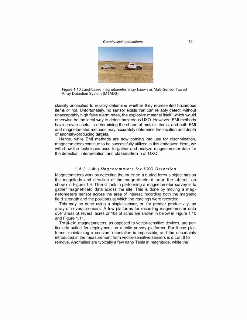
Figure 1.10 Land-based magnetometer array known as Multi-Sensor Towed Array Detection System (MTADS)

classify anomalies to reliably determine whether they represented hazardous items or not. Unfortunately, no sensor exists that can reliably detect, without unacceptably high false alarm rates, the explosive material itself, which would otherwise be the ideal way to detect hazardous UXO. However, EMI methods have proven useful in determining the shape of metallic items, and both EMI and magnetometer methods may accurately determine the location and depth of anomaly-producing targets.

Hence, while EMI methods are now coming into use for discrimination, magnetometers continue to be successfully utilized in this endeavor. Here, we will show the techniques used to gather and analyze magnetometer data for the detection, interpretation, and classication n of UXO.

1 . 5 . 3 Using Ma g ne t om e t e r s f o r U X O De t e c t i on Magnetometers work by detecting the inuence a buried ferrous object has on the magnitude and direction of the magneticeld d near the object, as shown in Figure 1.9. Therst task in performing a magnetometer survey is to gather magneticeld data across the site. This is done by moving a mag-netometers sensor across the area of interest, recording both the magnetic field strength and the positions at which the readings were recorded.

This may be done using a single sensor, or, for greater productivity, an array of several sensors. A few platforms for recording magnetometer data over areas of several acres or 10s of acres are shown in below in Figure 1.10 and Figure 1.11.

Total-eld magnetometers, as opposed to vector-sensitive devices, are par-ticularly suited for deployment on mobile survey platforms. For these plat-forms, maintaining a constant orientation is impossible, and the uncertainty introduced in the measurement from vector-sensitive sensors is dicult lt to remove. Anomalies are typically a few nano Tesla in magnitude, while the

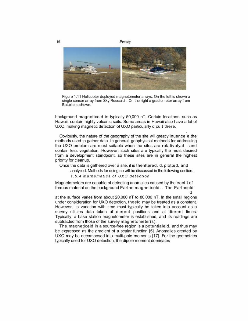
Figure 1.11 Helicopter deployed magnetometer arrays. On the left is shown a single sensor array from Sky Research. On the right a gradiometer array from Battelle is shown.

background magneticeld is typically 50,000 nT. Certain locations, such as Hawaii, contain highly volcanic soils. Some areas in Hawaii also have a lot of UXO, making magnetic detection of UXO particularly dicult there.

. Obviously, the nature of the geography of the site will greatly inuence e the

methods used to gather data. In general, geophysical methods for addressing the UXO problem are most suitable when the sites are relativelyat t and contain less vegetation. However, such sites are typically the most desired from a development standpoint, so these sites are in general the highest priority for cleanup.

Once the data is gathered over a site, it is thenltered, d, plotted, and analyzed. Methods for doing so will be discussed in the following section. 1 . 5 . 4 Ma t he m a t i c s of UX O det e c t i on

Magnetometers are capable of detecting anomalies caused by the eect t of ferrous material on the background Earths magneticeld. . The Earthseld

d at the surface varies from about 20,000 nT to 80,000 nT. In the small regions under consideration for UXO detection, theeld may be treated as a constant. However, its variation with time must typically be taken into account as a survey utilizes data taken at dierent positions and at dierent times. Typically, a base station magnetometer is established, and its readings are subtracted from those of the survey magnetometer(s).

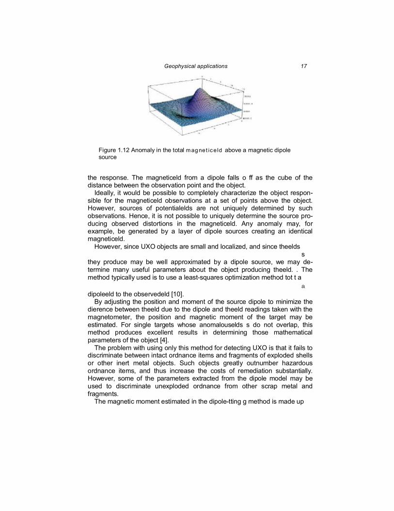
The magneticeld in a source-free region is a potentialeld, and thus may be expressed as the gradient of a scalar function [5]. Anomalies created by UXO may be decomposed into multi-pole moments [17]. For the geometries typically used for UXO detection, the dipole moment dominates

Geophysical applications 17

Figure 1.12 Anomaly in the total m agnet ice ld above a magnetic dipole source

the response. The magneticeld from a dipole falls o ff as the cube of the distance between the observation point and the object.

Ideally, it would be possible to completely characterize the object respon-sible for the magneticeld observations at a set of points above the object. However, sources of potentialelds are not uniquely determined by such observations. Hence, it is not possible to uniquely determine the source pro-ducing observed distortions in the magneticeld. Any anomaly may, for example, be generated by a layer of dipole sources creating an identical magneticeld.

However, since UXO objects are small and localized, and since theelds s

they produce may be well approximated by a dipole source, we may de-termine many useful parameters about the object producing theeld. . The method typically used is to use a least-squares optimization method tot t a

a dipoleeld to the observedeld [10].

By adjusting the position and moment of the source dipole to minimize the dierence between theeld due to the dipole and theeld readings taken with the magnetometer, the position and magnetic moment of the target may be estimated. For single targets whose anomalouselds s do not overlap, this method produces excellent results in determining those mathematical parameters of the object [4].

The problem with using only this method for detecting UXO is that it fails to discriminate between intact ordnance items and fragments of exploded shells or other inert metal objects. Such objects greatly outnumber hazardous ordnance items, and thus increase the costs of remediation substantially. However, some of the parameters extracted from the dipole model may be used to discriminate unexploded ordnance from other scrap metal and fragments.

The magnetic moment estimated in the dipole-tting g method is made up

18 Prouty

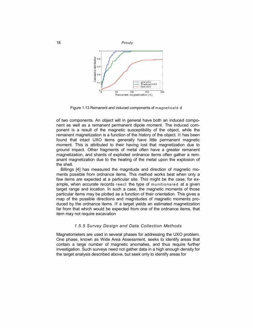
Figure 1.13 Remanent and induced components of m agnet ice ld d

of two components. An object will in general have both an induced compo-nent as well as a remanent permanent dipole moment. The induced com-ponent is a result of the magnetic susceptibility of the object, while the remanent magnetization is a function of the history of the object. I t has been found that intact UXO items generally have little permanent magnetic moment. This is attributed to their having lost that magnetization due to ground impact. Other fragments of metal often have a greater remanent magnetization, and shards of exploded ordnance items often gather a rem-anant magnetization due to the heating of the metal upon the explosion of the shell.

Billings [4] has measured the magnitude and direction of magnetic mo-ments possible from ordnance items. This method works best when only a few items are expected at a particular site. This might be the case, for ex-ample, when accurate records reect the type of muni t ionsred at a given target range and location. In such a case, the magnetic moments of those particular items may be plotted as a function of their orientation. This gives a map of the possible directions and magnitudes of magnetic moments pro-duced by the ordnance items. I f a target yields an estimated magnetization far from that which would be expected from one of the ordnance items, that item may not require excavation

1.5.5 Survey Design and Data Collection Methods

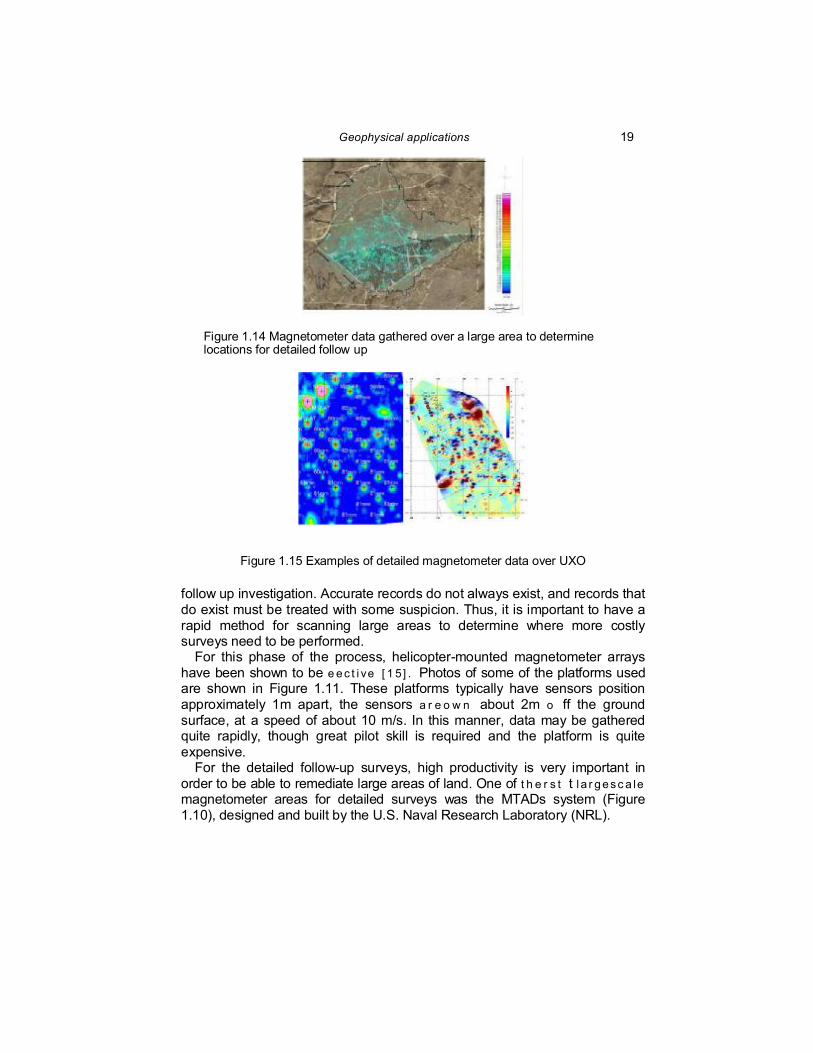
Magnetometers are used in several phases for addressing the UXO problem. One phase, known as Wide Area Assessment, seeks to identify areas that contain a large number of magnetic anomalies, and thus require further investigation. Such surveys need not gather data in a high enough density for the target analysis described above, but seek only to identify areas for

Geophysical applications 19

Figure 1.14 Magnetometer data gathered over a large area to determine locations for detailed follow up

Figure 1.15 Examples of detailed magnetometer data over UXO

follow up investigation. Accurate records do not always exist, and records that do exist must be treated with some suspicion. Thus, it is important to have a rapid method for scanning large areas to determine where more costly surveys need to be performed.

For this phase of the process, helicopter-mounted magnetometer arrays have been shown to be e ec t i ve [ 1 5] . Photos of some of the platforms used are shown in Figure 1.11. These platforms typically have sensors position approximately 1m apart, the sensors a r e o w n about 2m o ff the ground surface, at a speed of about 10 m/s. In this manner, data may be gathered quite rapidly, though great pilot skill is required and the platform is quite expensive.

For the detailed follow-up surveys, high productivity is very important in order to be able to remediate large areas of land. One of t h e r s t t l a r gesc a le magnetometer areas for detailed surveys was the MTADs system (Figure 1.10), designed and built by the U.S. Naval Research Laboratory (NRL).

20 Prouty

References

[1] 2004. Report of the Sefense Science Board Task Force on Unexploded Ordnance. Tech. rept. Defense Science Board.

[2] Alexandrov, E.B. 2004. Three-component variometer based on a scalar potas-sium sensor. Meas. Sci. Technol., 15, 918.

[3] Auster, H.U. 2007. Automation of absolute measurement of the geomagnetic eld. . Earth Planets Space, 59, 1007.

[4] Billings, S.D. 2004. Discrimination and classication of buried unexploded ordnance using magnetometry. IEEE Transactions on Geoscience and Remote Sensing, 42(6), 1241 - 1251.

[5] Blakely, Richard J. 1995. Potential Theory in Gravity and Magnetic Applications. New York: Cambridge University Press.

[6] Fairweather, A.J. 1072. A vector rubidium magnetometer. J Phys. E., 5, 986. [7] Gravrand, O. 2001. On the calibration of vectorial 4He pumped magnetometer.

Earth Planets Space, 53, 949. [8] Lamden, R.J. 1969. The design of unattended stations for recording geomag-

netic microsuplation signals. Journal of Phys E, 2, 125. [9] Llopis, J.L. 2008. Introduction to this UXO Special Issue of JEEG. Journal of

Environmental & Engineering Geophysics, 13(3), v. [10] M. Tchernychev, D.D. Snyder. 2007. Open source magnetic inversion program-

ming framework and its practical applications. Journal of Applied Physics, 61, 184 - 193.

[11] Nambighian, M.N. 2005. The historical development of the magnetic method in exploration. Geophysics, 70(6).

[12] Pulz, E. 2009. A quasi absolute optically pumped magnetometer for the per-manent recording of the Earths magneticeld d vector. Page 216 of: Proceedings of the X I IAGA Workshop on Geomagnetic Observatory Instruments. U.S. Geological Survey Open-File Report.

[13] Rasson, J.L. 1991. Geophys. Trans, 36, 187. [14] Rasson, J.L. 2009. Automatic D I u x Measurements with AUTODIF. Page 220

of: Proceedings of the X I IAGA Workshop on Geomagnetic Observatory Instruments, vol. 2009-1226. U.S. Geological Survey Open-File Report.

[15] S. Billings, D. Wright. 2010. Interpretation of high-resolution low-altitude he-licopter magnetometer surveys over sites contaminated with unexploded ord-nance. Journal of Applied Physics, doi:10.1016/j.jappgeo.2010.09.005.

[16] Smekalova, T. 2005. Magnetometric investigations of stone constructions within large ancient barrows of Denmark and Crimea. Geoarchaeology, 20(5), 461 - 482.

[17] Stratton, J. 1941. Electromagnetic Theory. New York: McGraw-Hill. [18] Telford, W.M. 1976. Applied Geophysics. Cambridge: Cambridge University

Press. [19] Vershovskii, A.K. 2006. Fast three-component magnetometer-variometer based

on a cesium sensor. Technical Physics, 51(1), 112. [20] Vershovskii, A.K. 2011. Optically Pumped Quantum Magnetometer Employing

Optically pumped quantum magnetometer employing two components of a magnetic precession signal. Technical Physics Letters, 37, 140.