instructor guide chapter 3 microfossils and biostra tigraphy · 2017-10-20 · chapter 3....

Ch 3 Microfossils and Biostratigraphy Instructor Guide

of 44

INSTRUCTOR GUIDE Chapter 3 Microfossils and Biostratigraphy

SUMMARY Microfossils are important, and in places the dominant constituents of deep sea sediments (see Chapter 2). The shells/hard parts of calcareous microfossils can be geochemically analyzed, for example by stable isotopes of oxygen and carbon, which are powerful proxies (indirect evidence) in paleoceanography and climate change studies (see Chapter 6). Microfossil evolution has provided a rich archive for establishing relative time in marine sedimentary sequences. In this chapter you will gain experience using microfossil distributions in deep-sea cores to apply a biostratigraphic zonation and interpret relative age, correlate from one region of the world ocean to another, and calculate rates of sediment accumulation. In Part 3.1, you will learn about the major types of marine microfossils and their habitats; you will consider their role in primary productivity in the world oceans, their geologic record and diversity through time, as well as the relationship between microfossil diversity and sea level changes through time. In Part 3.2, you will explore microfossil distribution in a deep-sea core and consider microfossils as age indicators. In Part 3.3, you will apply microfossil first and last occurrences (datum levels) in a deep-sea core to establish biostratigraphic zones. In Part 3.4, you will use these same microfossil datum levels to determine sediment accumulation rates. In Part 3.5, you will explore the reliability of microfossil datum levels in multiple locations.

Goal:

to gain experience with the use of microfossil evolution in establishing relative time.

Objectives:

1. Infer paleoecological and

After completing this exercise your students should be able to:

paleobiological information using microfossil distribution data.

2. Make observations about microfossil abundance data and make hypotheses to explain their observations.

3. Apply a biostratigraphic zonation to microfossil abundance data and use it to interpret relative ages.

4. Use microfossil data to calculate rates of sediment accumulation.

5. Use microfossil data to test the reliability of microfossil datum levels in multiple locations, and correlate sedimentary sequences at different locations.

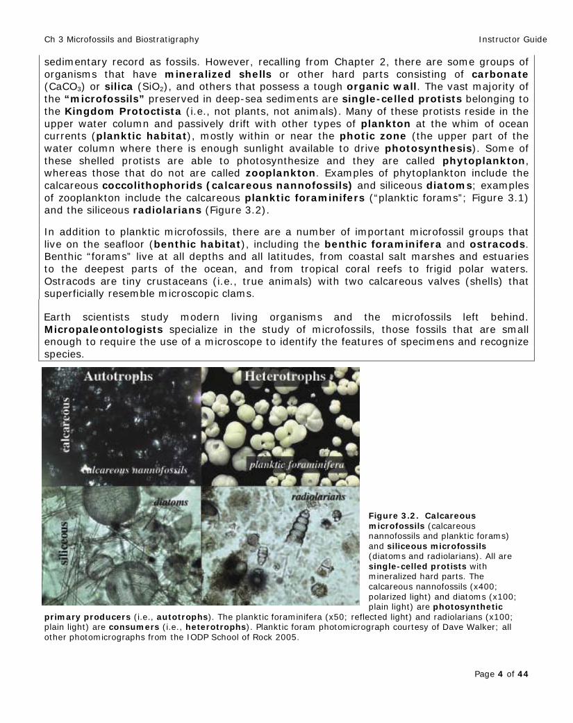
FIGURE 3.1. Four species of planktic foraminifers from the tropical western Atlantic: upper left: Globigerinoides ruber, upper right: Globigerinoides sacculifer, lower left: Globorotalia menardii, lower right: Neogloboquadrina dutertrei. Scale bar=100 µm (100 µm=0.1 mm). Photo courtesy of Mark Leckie.


of 44

I. How Can I Use All or Parts of this Exercise in my Class? (based on Project 2061 instructional materials design.)

Part 3.1 Part 3.2 Part 3.3 Part 3.4 Part 3.5

Title (of each part) What are Microfossils?

Microfossils in Deep Sea Sediment

Application of First & Last Occurrences

Sediment Accumulation Rates

Datum Reliability

How much class time will I need? (per part)

30-45 minutes

<30 minutes ~30 minutes, plus discussion time

<30 minutes <30 minutes

Can this be done independently (i.e., as homework)?

Yes, but doing Part 3.1 in lecture works well

Yes, as homework, lab or discussion section




What content will students be introduced to in this exercise? Phyto- & zooplankton distributions, abundances & diversity

X X X X X

Geologic timescale and/or Geomagnetic polarity timescale

X X X

Sea level change X Trophic levels & productivity X Age determination using fossils, index fossils, biozones, datums, first/last occurrences

X X X X

Extinction X X X X Sed accum rates, age-depth plots

X X

Calibration & correlation of different types of data

X X

Unconformities, hiatus X X Reliability and uncertainty X What types of transportable skills will students practice in this exercise? Make observations (describe what you see)

X X X X X

Plot data, determine lines of best fit, interpret graphs, diagrams, photos, tables

X X X X

Pose hypotheses or predictions X X X X X Perform calculations & develop quantitative skills

X X

Decision-making, problem solving & pattern recognition

X X X X X

What general prerequisite knowledge & skills are required?

Basic biology and Earth science



Basic math and Earth science

Basic geography and Earth science

What Anchor Exercises (or Parts of Exercises) should be done prior to this to guide student interpretation & reasoning?

Ch. 2: Seafloor Sediments

Part 3.1 Parts 3.1-3.2 Parts 3.1-3.3 Parts 3.1-3.4


of 44

II. Annotated Student Worksheets (i.e., the ANSWER KEY)

This section includes the annotated copy of the student worksheets with answers for each Part of this Chapter. This instructor guide contain the same sections as in the student book chapter, but also includes additional information such as: useful tips, discussion points, notes on places where students might get stuck, what specific points students should come away with from an exercise so as to be prepared for further work, as well as ideas and/or material for mini-lectures.

Part 3.1. What are Microfossils? Why are they Important in Climate Change Science?

WHAT ARE MICROFOSSILS? While there are many types of tiny animals and microorganisms living in the sunlit surface waters of the ocean, at depth in the water column and on the seafloor, most of these organisms do not possess the hard parts necessary for them to be preserved on the

What other resources or materials do I need? (e.g., internet access to show on-line video; access to maps, colored pencils)

None Access to world map or ocean floor map

None None Access to world map or ocean floor map

What student misconception does this exercise address?

Kingdoms of life; how productivity works

Evolution of life (first and last occurrences of organisms)

How relative age is assigned to (deep-sea) sediments

How age-depth plots are constructed

Dispersal of species; science is testable

What forms of data are used in this? (e.g., graphs, tables, photos, maps)

Photos, graphs

Photos, map, tables

Diagram, chart, tables

Tables, graph

Map, tables

What geographic locations are these datasets from?

N/A Western equatorial Pacific, NW Pacific – Shatsky Rise

NW Pacific – Shatsky Rise, North Pacific Ocean

NW Pacific – Shatsky Rise, eastern equatorial Pacific

NW Pacific – Shatsky Rise, Caribbean Sea

How can I use this exercise to identify my students’ prior knowledge (i.e., student misconceptions, commonly held beliefs)?

Prior knowledge and misconceptions can be identified by examining student answers of open ended questions and/or though class discussion. Student ideas on evolution, correlation, reliability will certainly be drawn out in this exercise.

How can I encourage students to reflect on what they have learned in this exercise? [Formative Assessment]

Exercise Parts can be concluded by asking: On note card (with or without name) to turn in, answer: What did you find most interesting/helpful in the exercise we did above? Does what we did model scientific practice? If so, how and if not, why not?

How can I assess student learning after they complete all or part of the exercise? [Summative Assessment]

See suggestions in Summative Assessment section below.

Where can I go to for more information on the science in this exercise?

See the Supplemental Materials and Reference sections below.


of 44

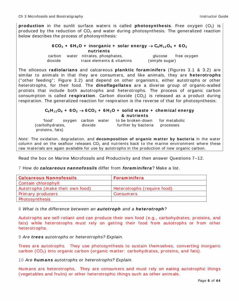
sedimentary record as fossils. However, recalling from Chapter 2, there are some groups of organisms that have mineralized shells or other hard parts consisting of carbonate (CaCO3) or silica (SiO2), and others that possess a tough organic wall. The vast majority of the “microfossils” preserved in deep-sea sediments are single-celled protists belonging to the Kingdom Protoctista (i.e., not plants, not animals). Many of these protists reside in the upper water column and passively drift with other types of plankton at the whim of ocean currents (planktic habitat), mostly within or near the photic zone (the upper part of the water column where there is enough sunlight available to drive photosynthesis). Some of these shelled protists are able to photosynthesize and they are called phytoplankton, whereas those that do not are called zooplankton. Examples of phytoplankton include the calcareous coccolithophorids (calcareous nannofossils) and siliceous diatoms; examples of zooplankton include the calcareous planktic foraminifers (“planktic forams”; Figure 3.1) and the siliceous radiolarians (Figure 3.2). In addition to planktic microfossils, there are a number of important microfossil groups that live on the seafloor (benthic habitat), including the benthic foraminifera and ostracods. Benthic “forams” live at all depths and all latitudes, from coastal salt marshes and estuaries to the deepest parts of the ocean, and from tropical coral reefs to frigid polar waters. Ostracods are tiny crustaceans (i.e., true animals) with two calcareous valves (shells) that superficially resemble microscopic clams.

Earth scientists study modern living organisms and the microfossils left behind. Micropaleontologists specialize in the study of microfossils, those fossils that are small enough to require the use of a microscope to identify the features of specimens and recognize species.

Figure 3.2. Calcareous microfossils (calcareous nannofossils and planktic forams) and siliceous microfossils (diatoms and radiolarians). All are single-celled protists with mineralized hard parts. The calcareous nannofossils (x400; polarized light) and diatoms (x100; plain light) are photosynthetic

primary producers (i.e., autotrophs). The planktic foraminifera (x50; reflected light) and radiolarians (x100; plain light) are consumers (i.e., heterotrophs). Planktic foram photomicrograph courtesy of Dave Walker; all other photomicrographs from the IODP School of Rock 2005.


of 44

1 In Chapter 2, Seafloor Sediments, you learned that there are a variety of marine microfossils found in deep-sea sediments. Why are microfossils found in deep-sea sediments? Explain.

Some marine organisms such as some groups of plankton have mineralized hard parts (shells or tests), composed of CaCO3 or SiO2. When these organisms are eaten or die, they “rain down” to the seafloor as individual shells, or aggregates or in fecal pellets of larger organisms and are preserved into the sedimentary record. They are buried by more microfossils or other types of sediment over time.

Trophic Levels and Productivity

2 What types of organisms make up the base of the food chain (i.e., food webs, food pyramids) on land?

Plants 3 Why are these organisms at the base of the food chain?

They create their own food through photosynthesis and are therefore consumed by other organisms that cannot make their own food; i.e., plants are autotrophs and primary producers.

4 What types of organisms make up the base of the food chain in the ocean?

In the surface ocean, phytoplankton are the base of the food chain (and photosynthetic bacteria called cyanobacteria) 5 How might these organisms be similar, and how might they differ from those on land?

They are similar in that they are both autotrophs and can produce their own nutrition from inorganic material through photosynthesis.

They differ in that phytoplankton can only produce food within the photic zone, or upper ~100-150 m of the water column. Also, phytoplankton are very tiny compared to land plants.

6 It is very cold and pitch black on the seafloor below 1000 m water depth. Speculate about the types of organisms that make up the base of the food chain in the deep ocean. Chemosynthetic bacteria and archea, e.g., associated with hydrothermal vents at spreading centers and methane seeps along continental margins MARINE MICROFOSSILS AND PRODUCTIVITY The siliceous diatoms and calcareous coccolithophorids (and other calcareous nannofossils) are similar to plants, in that they contain chlorophyll and, like plants, they are autotrophs (“self-feeding”; Figure 3.2). These autotrophs synthesize organic molecules (e.g., carbohydrates, proteins, and fats) from inorganic molecules (CO2, water, and nutrients) using solar radiation. In other words, they make organic carbon from inorganic carbon. Such organisms are considered to be primary producers because they manufacture the organic materials that other types of organism require as food; thus, primary producers form the basis of many marine food chains/food pyramids. The process of organic carbon


of 44

production in the sunlit surface waters is called photosynthesis. Free oxygen (O2) is produced by the reduction of CO2 and water during photosynthesis. The generalized reaction below describes the process of photosynthesis:

6CO2 + 6H2O + inorganic + solar energy → C6H12O6 + 6O2 nutrients carbon water nitrates, phosphates, glucose free oxygen dioxide trace elements & vitamins (simple sugar) The siliceous radiolarians and calcareous planktic foraminifers (Figures 3.1 & 3.2) are similar to animals in that they are consumers, and like animals, they are heterotrophs (“other feeding”; Figure 3.2) and depend on other organisms, either autotrophs or other heterotrophs, for their food. The dinoflagellates are a diverse group of organic-walled protists that include both autotrophs and heterotrophs. The process of organic carbon consumption is called respiration. Carbon dioxide (CO2) is released as a product during respiration. The generalized reaction for respiration is the reverse of that for photosynthesis:

C6H12O6 + 6O2 → 6CO2 + 6H2O + solid waste + chemical energy & nutrients

‘food’ oxygen carbon water to be broken-down for metabolic (carbohydrates, dioxide further by bacteria processes proteins, fats) Note: The oxidation, degradation, and decomposition of organic matter by bacteria in the water column and on the seafloor releases CO2 and nutrients back to the marine environment where these raw materials are again available for use by autotrophs in the production of new organic carbon. Read the box on Marine Microfossils and Productivity and then answer Questions 7–12. 7 How do calcareous nannofossils differ from foraminifera? Make a list. Calcareous Nannofossils Foraminifera Contain chlorophyll Autotrophs (make their own food) Heterotrophs (require food) Primary producers Consumers Photosynthesis 8 What is the difference between an autotroph and a heterotroph?

Autotrophs are self-reliant and can produce their own food (e.g., carbohydrates, proteins, and fats) while heterotrophs must rely on getting their food from autotrophs or from other heterotrophs.

9 Are trees autotrophs or heterotrophs? Explain.

Trees are autotrophs. They use photosynthesis to sustain themselves, converting inorganic carbon (CO2) into organic carbon (organic matter: carbohydrates, proteins, and fats).

10 Are humans autotrophs or heterotrophs? Explain.

Humans are heterotrophs. They are consumers and must rely on eating autotrophic things (vegetables and fruits) or other heterotrophic things such as other animals.


of 44

11 Why is photosynthesis a fundamentally important Earth systems process?

It is the mechanism by which phytoplankton, cyanobacteria, algae, plants, and trees thrive. Without it, we wouldn’t have oxygen on Earth, which is such a vital by-product of photosynthesis. It makes up the base of the food chain that many animals rely on. It also has a fundamental impact on climate. Photosynthesis draws down CO2 from the atmosphere; vegetation and soils on land, and phytoplankton and deep-sea sediments in the ocean are important sinks for CO2.

12 The global carbon cycle describes the exchange of different types of carbon compounds (e.g., CO2, organic carbon, CaCO3) between the various carbon reservoirs (e.g., atmosphere, biosphere, ocean, solid Earth) in the Earth system (see Chapter 5). Speculate how changes in photosynthesis might have an impact on the carbon cycle and therefore the global climate. Vegetation and phytoplankton draw down CO2 from the atmosphere through photosynthesis, which could lead to global cooling if the rate of photosynthesis or organic carbon burial increased. If photosynthesis were to decrease, then CO2 would increase in the atmosphere resulting in global warming.

Marine Microfossils of the Mesozoic and Cenozoic Eras

The major mineralized microfossil groups have geologic records that extend back more than 100 millions years (Figures 3.3 & 3.4); in fact, the radiolarians are found in marine rocks dating back to 540 million years ago! Microfossils are very useful in scientific ocean drilling and in the oil and gas industry because their tiny size and great abundance in marine sediments allows geoscientists to reconstruct ancient environmental conditions, establish the relative age of the sedimentary layers (i.e., fossils found in lower or deeper strata are older than fossils found in higher or shallower strata; fossil occurrences can be used to identify the relative order of past events), and correlate the sedimentary layers with other localities around the world.


of 44

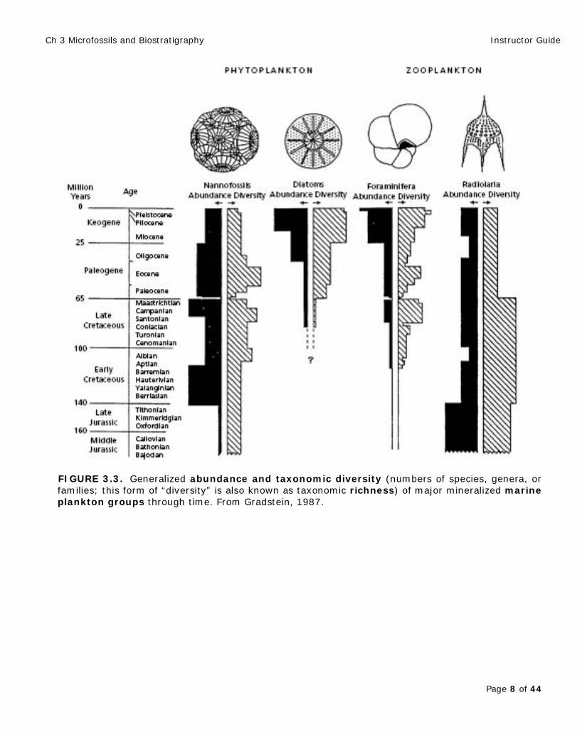
FIGURE 3.3. Generalized abundance and taxonomic diversity (numbers of species, genera, or families; this form of “diversity” is also known as taxonomic richness) of major mineralized marine plankton groups through time. From Gradstein, 1987.


of 44

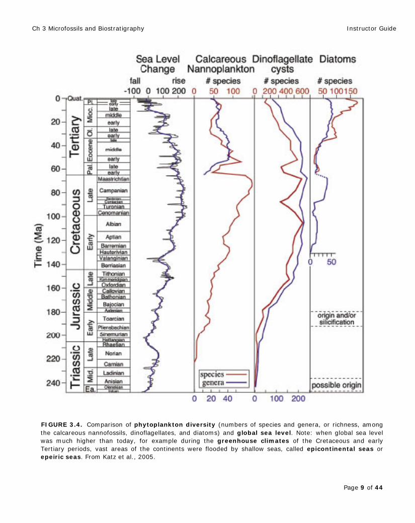
FIGURE 3.4. Comparison of phytoplankton diversity (numbers of species and genera, or richness, among the calcareous nannofossils, dinoflagellates, and diatoms) and global sea level. Note: when global sea level was much higher than today, for example during the greenhouse climates of the Cretaceous and early Tertiary periods, vast areas of the continents were flooded by shallow seas, called epicontinental seas or epeiric seas. From Katz et al., 2005.


of 44

13 Consider diversity (i.e., numbers of species and numbers of genera) through the Mesozoic and Cenozoic Eras (Figures 3.3 & 3.4). In very general terms, describe the pattern of evolution (i.e., times of increasing or decreasing diversity) of each of the following groups of microfossils:

(a) Calcareous nannofossils - Major radiation throughout Jurassic and Cretaceous; radiation in the early Paleogene and minor radiation in the Neogene - Gradually increased from the Triassic to the end of the Cretaceous - Abruptly declined at the K/Pg boundary - Abrupt increase at the PETM followed by a gradual decline through remainder of the Cenozoic

(b) Diatoms

- Minor radiations in the mid-Cretaceous and Late Cretaceous; major radiations in the Eocene and Neogene - Gradual increase from the Early Cretaceous followed by a slight decline at the Albian-Cenomanian boundary - Abrupt increase at the Campanian followed by a rapid decrease at the K/Pg boundary - Increase at the end of the Eocene and again during the Neogene

(c) Dinoflagellates

- Major radiation in Late Jurassic through mid-Cretaceous, Late Cretaceous, and early Paleogene - Gradual increase from the Triassic to mid-Albian - Abrupt decline at the Coniacian followed by a rapid increase to the mid-Maastrichtian - Abrupt decrease at the K/Pg boundary followed by an abrupt increase to the PETM where it declines gradually after

(d) Planktic Foraminifers

- 3 or 4 major radiations: mid-Cretaceous, Late Cretaceous, Paleogene, and Neogene - Rapid increase from the Coniacian to the K/Pg boundary - Abrupt decrease at the K/Pg boundary followed by an increase to the end of the Eocene - A gradual increase from the Oligocene to the present

(e) Radiolarians

- High diversity from the middle Jurassic to the K/Pg boundary - Abrupt decline in diversity at the K/Pg boundary

14 Are there any similarities in the diversity patterns between any of the groups? If so, describe. - All show a major decrease in diversity at the K/Pg boundary, especially the calcareous plankton: calcareous nannofossils and planktic forams - All show an increase in diversity (except radiolarians) at the PETM - All show a general gradual increase in diversity leading up to the Cretaceous


of 44

15 Do phytoplankton and zooplankton groups track each other? Explain. Yes, in general. Zooplankton abundances rely on phytoplankton as a food source.

16 Based on Figure 3.4, are there any similarities between the pattern of plankton

Diversity and global sea level change? If so, describe.

Yes – in general, plankton diversity parallels changes is sea level, particularly during the Mesozoic and Paleogene. However, during the Neogene, planktic foram and especially diatom diversity increases while global sea level is falling.

17 Hypothesize about why similarities between plankton diversity and global sea level might exist.

During times of high sea level and widespread shallow seas, phytoplankton are abundant and many diversify during the Mesozoic and early Paleogene; perhaps this is driven in part by more niche spaces available for diversification. Also global warmth and increased weathering rates may have provided increased nutrient availability in some marine environments.

Part 3.2. Microfossils in Deep-Sea Sediments

Consider this scenario: We have a core of deep-sea sediment from a known location that has been described and sampled. What else do you want to know about this core?

A next logical step is to make an age determination in order to provide a temporal context for the core. Without an age, it is very difficult to tell a story, geologic or otherwise (e.g., “Once upon a time . . . ”, or “Long, long ago in a galaxy far, far away . . . ”). Geoscientists depend on reliable age assignments in order to (1) calibrate paleomagnetic records and other types of geologic data against the geologic time scale, (2) calculate rates of sediment accumulation, and (3) correlate core intervals representing a specific time from one location to another around the world oceans.

1 List your ideas on how geoscientists determine the “age” of a sequence of sedimentary layers. This question could be addressed by students in a variety of ways: 1) think-pair-share, 2) small group, or classroom discussion, the latter featuring the instructor making a list on the board, overhead, or computer (projected on to a screen) based on student input. Another very effective variation is to have think-pair-share followed by a general classroom discussion. The result will be a list created from student input. As the list comes together in your classroom discussion, there may be opportunities for teachable moments. Some possible responses:

• Fossils (or microfossils) – you might ask how fossils can be used to determine the age of sediments.

• 14C dating – this is one of the most common replies and misconceptions in age dating. Many introductory students are very unfamiliar with the principles of radiometric age dating and the variety of radiometric dating techniques, but they’ve all ‘heard’ of 14C dating. You might ask what type of materials can actually be dated. 14C dating is


of 44

restricted to relatively young (<60,000 years) carbon-containing materials, including calcium carbonate.

• Magnetism (or paleomagnetism) – this will be explored and described in the next exercise module, but you might ask how magnetism-paleomagnetism can be used to determine the age of sediments. I suggest not going into much detail if you plan to also do the exercise module on paleomagnetism.

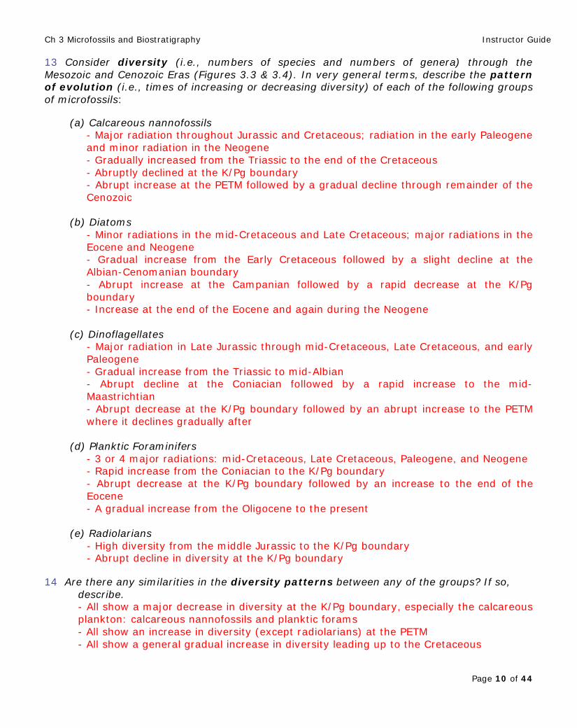
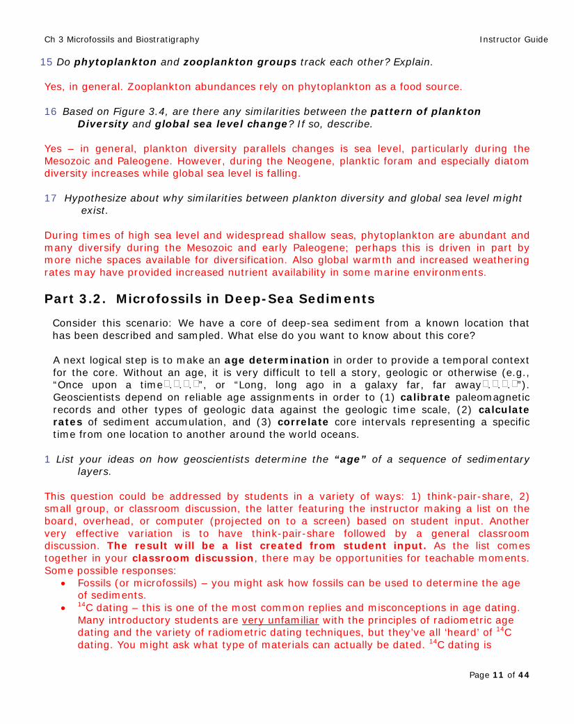
The above discussion will reveal the nature of your students’ existing knowledge about age determination. The “boxes” in these modules are brief snips of information that are useful background and provide additional context for the module. SMEAR SLIDES AND CALCAREOUS NANNOFOSSILS A smear slide is made to investigate the composition and texture of sediments (recall how you used smear slide data in Chapter 2 to determine sediment lithologies). To prepare a smear slide, a small amount of sediment from the core, collected with a toothpick, is mixed with a couple of drops of water to make a slurry (Figure 3.5). This slurry is smeared in a very thin layer across the glass slide, which is then dried on a hot plate. Adhesive and a cover slip are added. The adhesive is cured under a black light (UV radiation) for about 5 minutes. Now the slide is ready to be examined using a transmitted light microscope.

FIGURE 3.5. Making a smear slide. Note the sample label affixed to the glass slide describing exactly where this toothpick smear slide came from. Photo courtesy of Tina King. Micropaleontolgists specializing in calcareous nannofossils use a high-powered transmitted light microscope to study these very tiny microfossils (Figure 3.6). They typically work with magnifications of 1000–1400x and use different types of light to accentuate the subtle features of the calcite hard parts, including plane-polarized light, plane-polarized light with a phase contrast filter, and cross-polarized light.


of 44

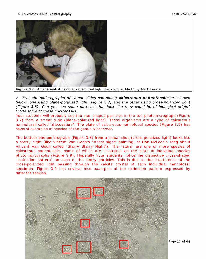
Figure 3.6. A geoscientist using a transmitted light microscope. Photo by Mark Leckie. 2 Two photomicrographs of smear slides containing calcareous nannofossils are shown below, one using plane-polarized light (Figure 3.7) and the other using cross-polarized light (Figure 3.8). Can you see some particles that look like they could be of biological origin? Circle some of these microfossils. Your students will probably see the star-shaped particles in the top photomicrograph (Figure 3.7) from a smear slide (plane-polarized light). These organisms are a type of calcareous nannofossil called “discoasters”. The plate of calcareous nannofossil species (Figure 3.9) has several examples of species of the genus Discoaster. The bottom photomicrograph (Figure 3.8) from a smear slide (cross-polarized light) looks like a starry night (like Vincent Van Gogh’s “starry night” painting, or Don McLean’s song about Vincent Van Gogh called “Starry Starry Night”). The “stars” are one or more species of calcareous nannofossils, some of which are illustrated on the plate of individual species photomicrographs (Figure 3.9). Hopefully your students notice the distinctive cross-shaped “extinction pattern” on each of the starry particles. This is due to the interference of the cross-polarized light passing through the calcite crystal of each individual nannofossil specimen. Figure 3.9 has several nice examples of the extinction pattern expressed by different species.


of 44

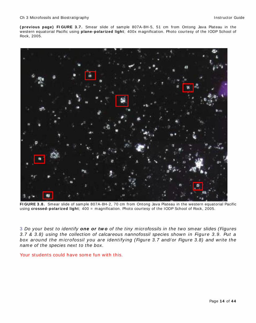
(previous page) FIGURE 3.7. Smear slide of sample 807A-8H-5, 51 cm from Ontong Java Plateau in the western equatorial Pacific using plane-polarized light; 400x magnification. Photo courtesy of the IODP School of Rock, 2005.

FIGURE 3.8. Smear slide of sample 807A-8H-2, 70 cm from Ontong Java Plateau in the western equatorial Pacific using crossed-polarized light; 400 = magnification. Photo courtesy of the IODP School of Rock, 2005.

3 Do your best to identify one or two of the tiny microfossils in the two smear slides (Figures 3.7 & 3.8) using the collection of calcareous nannofossil species shown in Figure 3.9. Put a box around the microfossil you are identifying (Figure 3.7 and/or Figure 3.8) and write the name of the species next to the box.

Your students could have some fun with this.


of 44

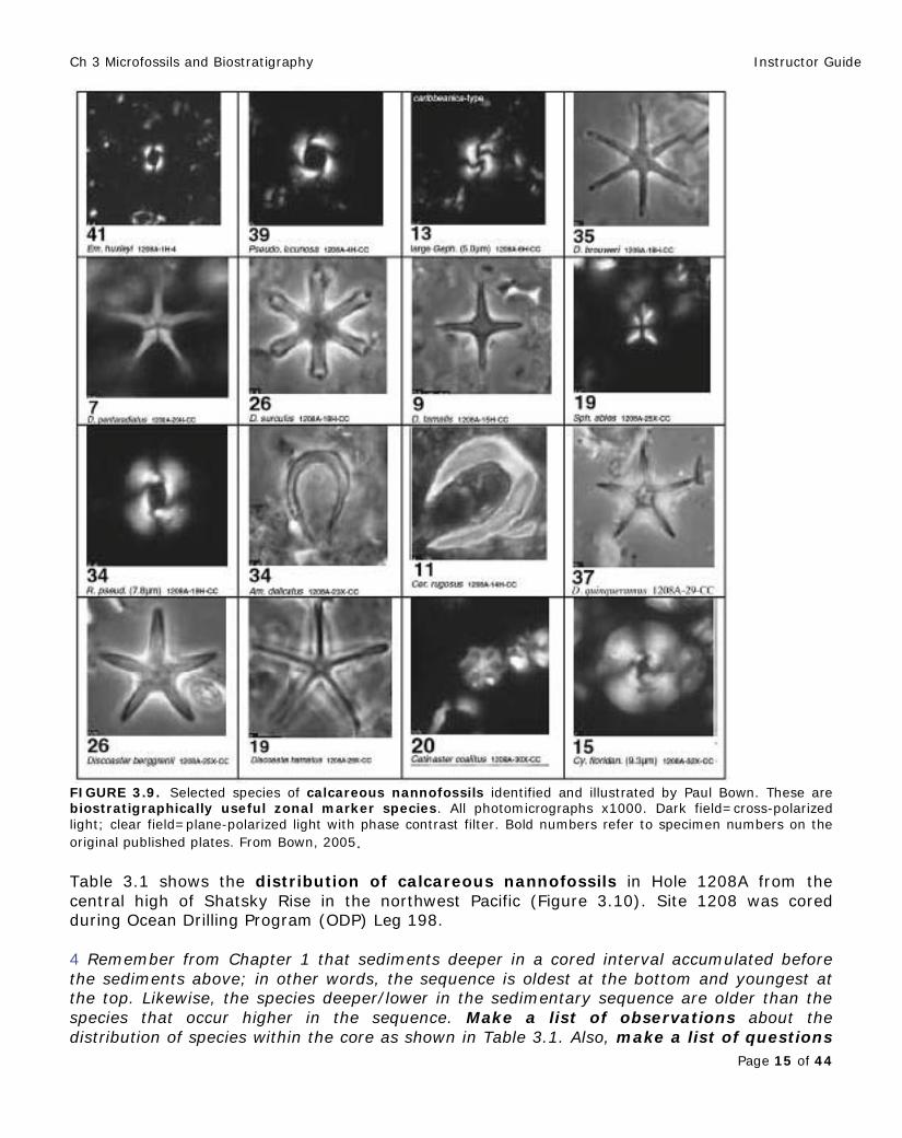
FIGURE 3.9. Selected species of calcareous nannofossils identified and illustrated by Paul Bown. These are biostratigraphically useful zonal marker species. All photomicrographs x1000. Dark field=cross-polarized light; clear field=plane-polarized light with phase contrast filter. Bold numbers refer to specimen numbers on the original published plates. From Bown, 2005. Table 3.1 shows the distribution of calcareous nannofossils in Hole 1208A from the central high of Shatsky Rise in the northwest Pacific (Figure 3.10). Site 1208 was cored during Ocean Drilling Program (ODP) Leg 198. 4 Remember from Chapter 1 that sediments deeper in a cored interval accumulated before the sediments above; in other words, the sequence is oldest at the bottom and youngest at the top. Likewise, the species deeper/lower in the sedimentary sequence are older than the species that occur higher in the sequence. Make a list of observations about the distribution of species within the core as shown in Table 3.1. Also, make a list of questions


of 44

that you may have about the distribution of species in this table. What additional information would you like to know about the species and their distribution in the Site 1208 drill site? Observations students may make:

• Species don’t occur in all samples. • There are many species in these samples. • Some species occur more-or-less persistently from one sample to the next and then

disappear • Some species are abundant or common in the samples, while other species are few or

rare. • Some species occur in the lower part of the sequence but not in the upper part, while

other species only occur in the upper part of the sequence. • The species in the sediment samples changes up-section (i.e., the species at this site

change over time) • Species of the genus Discoaster disappear above 100 mbsf.

It’s important to remind students that as they ‘read’ the table of microfossil data and make observations, the samples listed in the table come from sediments that accumulated layer by layer, with the oldest sediments and their contained microfossils at the bottom of this list of samples, and the youngest samples at the top. They might think of this sequence of sediment samples as a tape-recorder of geologic history; like pages in a book.

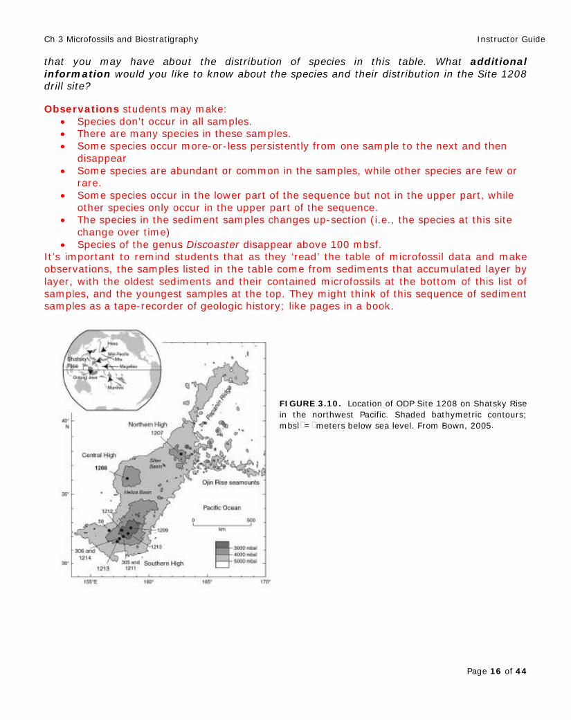
FIGURE 3.10. Location of ODP Site 1208 on Shatsky Rise in the northwest Pacific. Shaded bathymetric contours; mbsl = meters below sea level. From Bown, 2005.


of 44

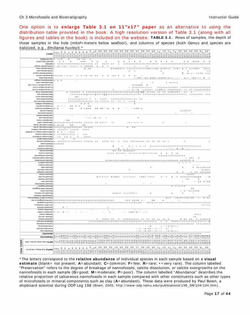
One option is to enlarge Table 3.1 on 11”x17” paper as an alternative to using the distribution table provided in the book. A high resolution version of Table 3.1 (along with all figures and tables in the book) is included on the website. TABLE 3.1. Rows of samples, the depth of those samples in the hole (mbsf=meters below seafloor), and columns of species (both Genus and species are italicized, e.g., Emiliania huxleyi).*

*The letters correspond to the relative abundance of individual species in each sample based on a visual estimate (blank= not present; A=abundant; C=common; F=few; R=rare; •=very rare). The column labelled “Preservation” refers to the degree of breakage of nannofossils, calcite dissolution, or calcite overgrowths on the nannofossils in each sample (G=good; M=moderate; P=poor). The column labelled “Abundance” describes the relative proportion of calcareous nannofossils in each sample compared with other constituents such as other types of microfossils or mineral components such as clay (A=abundant). These data were produced by Paul Bown, a shipboard scientist during ODP Leg 198 (Bown, 2005; http://www-odp.tamu.edu/publications/198_SR/104/104.htm).


of 44

Questions that students may have: • Why do some species come and go (i.e., why don’t they occur consistently from one

sample to the next)? • Why do some species show variability in abundance from one sample to the next? • Why do some species suddenly disappear up-section? • Why do other species suddenly appear in the section?

These are possible ‘teachable moments’ about ecology, paleoecology, and evolution. There are a number of different directions you could go from here. The exercises that follow will focus more on the application of these observations rather than the ecology of the organisms or processes of evolution.

Additional Information: The classroom discussion about this distribution table will generate a buzz. Is this site typical of the distribution of calcareous nannofossils in deep-sea sediments?

5 Fossil occurrences can be used to identify the relative order of past events. Geoscientists “read” the sedimentary record from bottom to top (i.e., from older to younger). How might the species data in Table 3.1 be useful for determining how old the sediment layers are in this drill site? Explain.

Microfossils may indicate age because: • Species have known geologic ranges (i.e., species evolve and become extinct;

species not living today existed for a finite time on Earth before becoming extinct). • Species ranges are known from a similar pattern of first occurrences (evolution)

and last occurrences (extinction) at multiple locations. • Species first and last occurrences are referred to as “datums”. • Species first and last occurrences, and their individual ranges are predictable and

testable. Students are not likely to grasp the concept of first and last occurrences, or a species stratigraphic range right away. The concepts listed above provide the teachable moment.

Part 3.3. Application of Microfossil First and Last Occurrences

The presence of microfossils in many types of deep-sea sediments provides a basis for determination of age. The recurrent (and testable) pattern of fossil first occurrences (FOs) and last occurrences (LOs) recognized by paleontologists studying sedimentary sequences reveals the relative sequence of evolutionary origination and extinction of species through time. In other words, in a distribution table showing the occurrences of species in a deep-sea core, like Table 3.1, the lowest occurrence of a species represents the first time (i.e., first occurrence, FO) this particular taxon was found in this area of the northwest Pacific. This can be considered the evolutionary first appearance, or time of origination of this new species. By contrast, the highest occurrence of a species represents the last time (i.e., last occurrence, LO) this particular taxon was found in this area. This can be considered the evolutionary last appearance, or time of extinction of this species. Because of these evolutionary events, microfossil species found in marine sediments are unique to a particular interval of geologic time and this property makes them very useful for age determination (Figure 3.11).


of 44

1 How can geoscientists test whether a pattern or sequence of fossil first and last occurrences is consistent and repeatable? We hope that the students would suggest that another deep-sea site should be investigated to see if the same sequence of first and last occurrences is present at more than one site. By the way, this is precisely the exercise developed in Part 5 (‘How reliable are microfossil datums?’). BIOSTRATIGRAPHY Biostratigraphy is the study of sedimentary layers based on fossil content. Paleontologists organize sedimentary layers into biozones based on the first and last occurrences of selected species; such zonal marker species (index fossils) are more suitable than other species for biostratigraphy, because they have short stratigraphic ranges, are geographically widespread, easily recognized, and well preserved. These levels of origination and extinction of marker species are called biostratigraphic datum levels. The ages of the biostratigraphic datum levels can be determined by multiple methods including paleomagnetic stratigraphy and radiometric age dating (this will be explored in Chapter 4, Paleomagnetism and Magnetostratigraphy).

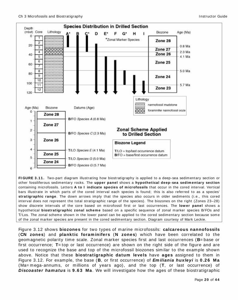
Zonal marker species are used to differentiate intervals of geologic time in a sedimentary section cored from the deep sea, thus essentially determining the age of successive layers of sediment. In the case illustrated in Figure 3.11, the distribution of eight microfossil species (A to I) is shown in a 120-meter cored interval. Four of these species (A, C, E, and G) have been established previously as zonal marker species because their first and/or last occurrences have been shown to be reliable biostratigraphic datum levels.


of 44

FIGURE 3.11. Two-part diagram illustrating how biostratigraphy is applied to a deep-sea sedimentary section or other fossiliferous sedimentary rocks. The upper panel shows a hypothetical deep-sea sedimentary section containing microfossils. Letters A to I indicate species of microfossils that occur in the cored interval. Vertical bars illustrate in which parts of the cored interval each species is found; this is also referred to as a species’ stratigraphic range. The down arrows imply that the species also occurs in older sediments (i.e., this cored interval does not represent the total stratigraphic range of the species). The biozones on the right (Zones 23–28) show discrete intervals of the core based on microfossil first or last occurrences. The lower panel shows a hypothetical biostratigraphic zonal scheme based on a specific sequence of zonal marker species B/FOs and T/Los. The zonal scheme shown in the lower panel can be applied to the cored sedimentary section because some of the zonal marker species are present in the cored sedimentary section. Diagram courtesy of Mark Leckie.

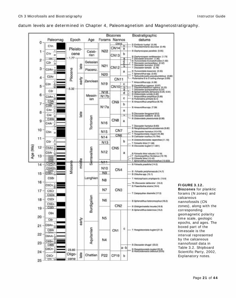
Figure 3.12 shows biozones for two types of marine microfossils: calcareous nannofossils (CN zones) and planktic foraminifers (N zones) which have been correlated to the geomagnetic polarity time scale. Zonal marker species first and last occurrences (B=base or first occurrence; T=top or last occurrence) are shown on the right side of the figure and are used to recognize the base and top of the microfossil biozones similar to the example shown above. Notice that these biostratigraphic datum levels have ages assigned to them in Figure 3.12. For example, the base (B, or first occurrence) of Emiliania huxleyi is 0.26 Ma (Ma=mega-annums, or millions of years ago), and the top (T, or last occurrence) of Discoaster hamatus is 9.63 Ma. We will investigate how the ages of these biostratigraphic


of 44

datum levels are determined in Chapter 4, Paleomagnetism and Magnetostratigraphy.

FIGURE 3.12. Biozones for planktic forams (N zones) and calcareous nannofossils (CN zones), along with the corresponding geomagnetic polarity time scale, geologic epochs, and ages. The boxed part of the timescale is the interval represented by the calcareous nannofossil data in Table 3.2. Shipboard Scientific Party, 2002, Explanatory notes.


of 44

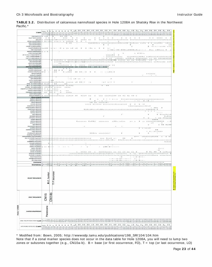
Table 3.2 shows is the distribution of calcareous nannofossil species in Hole 1208A on Shatsky Rise in the Northwest Pacific. This table is nearly identical with Table 3.1 and depicts the stratigraphic occurrence of species found in samples analyzed from Hole 1208A. The first column corresponds to a sample identifier (core-section, interval) and the second column is the depth in Hole 1208A (meters below seafloor, mbsf) for each of the samples. What is different about this version of the distribution table (compared to that shown in Table 3.1) is the addition of several columns: Geochronology, Nannofossil Zone, and Nannofossil Datum. These are to be filled in as part of this exercise. One option is to enlarge Table 3.2 on 11”x17” paper as an alternative to using the distribution table provided in the book. A high resolution version of Table 3.2 (along with all figures and tables in the book) is included on the website.


of 44

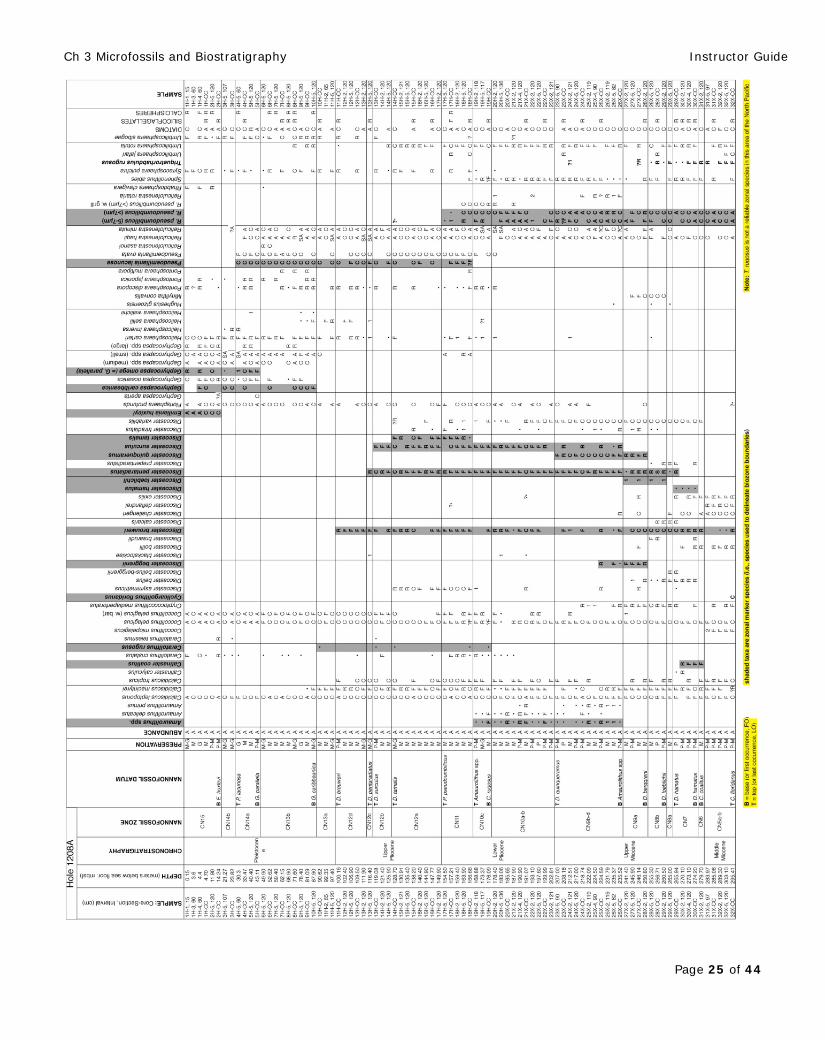
TABLE 3.2. Distribution of calcareous nannofossil species in Hole 1208A on Shatsky Rise in the Northwest Pacific.*

* Modified from: Bown, 2005; http://wwwodp.tamu.edu/publications/198_SR/104/104.htm Note that if a zonal marker species does not occur in the data table for Hole 1208A, you will need to lump two zones or subzones together (e.g., CN10a-b). B = base (or first occurrence, FO), T = top (or last occurrence, LO)


of 44

In this exercise you will interpret and apply the calcareous nannofossil zonal scheme (CN zones) presented in Figure 3.12 to the actual nannofossil distribution data from Hole 1208A (Table 3.2).

Step 1: Find the species of calcareous nannofossils that correspond with the CN zone boundaries shown in Figure 3.12; these are the zonal marker species (i.e., species names that line up with zone boundaries). Each zonal marker species will either be a base (B) or a top (T).

Step 2: Find each of these zonal marker species on the Hole 1208A distribution table on the following page. Be sure to note whether you need the base (first occurrence) or top (last occurrence) of the species range. Please note: some zonal species may not be present in the Hole 1208A data.

For example: The two youngest biozones are interpreted on Table 3.2: See previous page.

• The base, or first occurrence of Emiliania huxleyi (distribution highlighted in gray) is used to define the boundary between Zone CN14b and CN15. E. huxleyi first occurs in sample 2H-CC, so this sample is the lowest sample in Zone CN15. Draw a horizontal line across the distribution table between sample 2H-CC and the underlying sample 3H-5, 107 cm. This line represents the boundary between Zone CN14b and CN15. The age of this level in Hole 1208A is 0.26 Ma.

• The top, or last occurrence of Pseudoemiliania lacunosa (distribution highlighted in gray) is used to define the boundary between Zone CN14a and CN14b. P. lacunosa last occurs in sample 4H-5, 60, so this sample is the highest sample in Zone CN14a. Draw a horizontal line across the distribution table between sample 4H-5, 60 and the overlying sample 3H-CC. This line represents the boundary between Zone CN14a and CN14b. The age of this level in Hole 1208A is 0.46 Ma.

2 Interpret biozones for the remainder of the Hole 1208A distribution table (Table 3.2) by locating the CN zonal marker species and drawing horizontal lines on Table 3.2 corresponding with the zone boundaries. Fill in the columns of Table 3.2 for Geochronology, Nannofossil Zone, and Nannofossil Datum as shown for the two examples described above. Geochronology is a geologic time unit and refers to the Epoch/Age of the sediment (e.g., Pleistocene, late Pliocene, early Pliocene, late Miocene, middle Miocene).

Next page: Interpreted distribution table is shown on next page. Species highlighted in gray are the index (marker) species for the zones. Horizontal lines show the biozone boundaries.


of 44


of 44

3 In this investigation you learned how to apply a biostratigraphic zonal scheme to a cored sedimentary sequence from the seafloor of the North Pacific Ocean. This process essentially enabled you to convert depth to age for that sedimentary sequence. What does knowing “age” now allow you to explore about the history of environmental and climate change? For example: 1) to determine relative age of a fossiliferous sedimentary sequence (because some species have known or predictable first and last occurrences relative to other species), 2) to correlate from one location to another so that you can relate the sediments and their history of deposition from one place to another (need to do this to reconstruct geologic history), and 3) to calculate rates of sedimentation/sediment accumulation (Part 3 of this exercise), and other geologic processes provided you can determine the absolute age of the species first and last occurrences (this latter piece is described in detail in Chapter 4-Paleomagnetism/Magnetostratigraphy exercise module; see discussion of Geomagnetic Polarity Time Scale).

Part 3.4. Using Microfossil Datum Levels to Calculate Sedimentation Rates

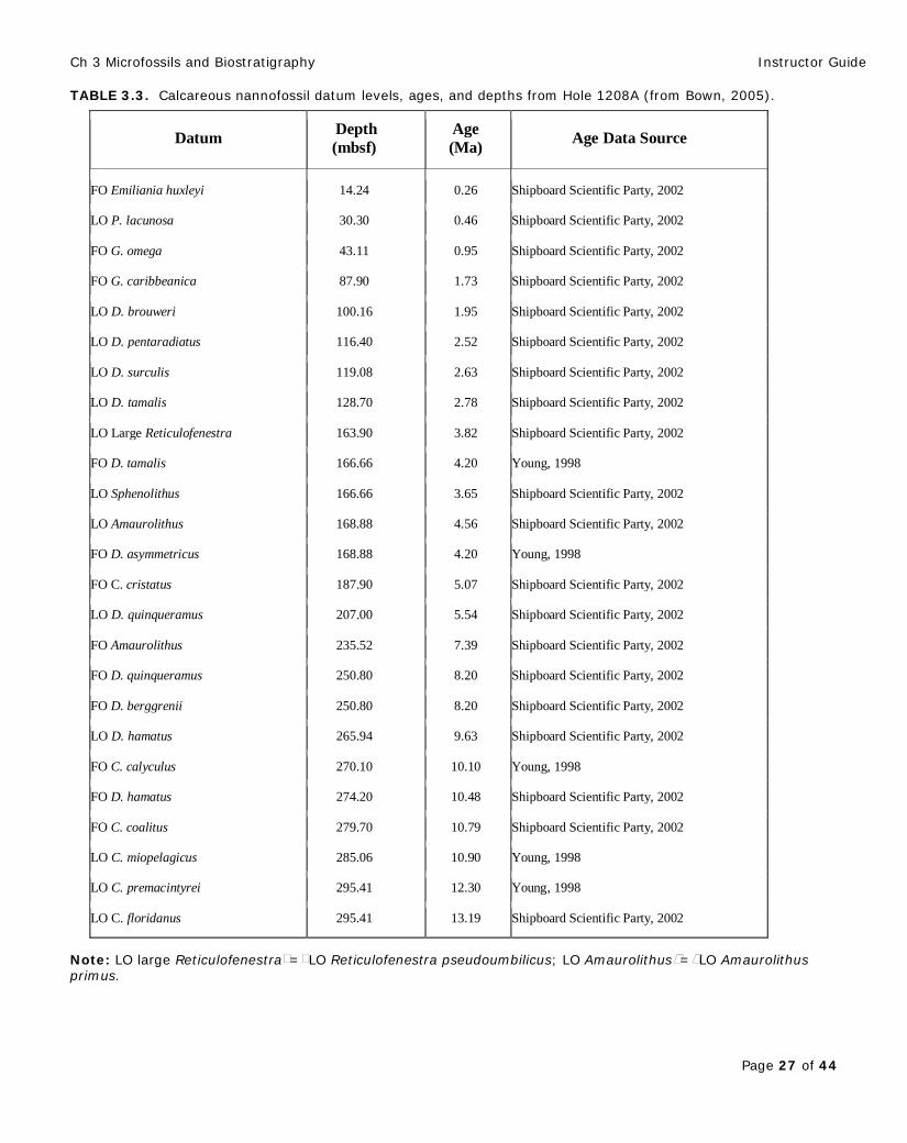
Table 3.3 [next page] presents a summary of select calcareous nannofossil species datum levels observed at Site 1208 (ODP Leg 198) on the central high of Shatsky Rise in the Northwest Pacific (from Bown, 2005). FO = first occurrence, LO = last occurrence. This list represents a subset of all the species shown on the distribution table (Tables 3.1 and 3.2) analyzed in Part 3.2 and Part 3.3 (i.e., most of these are the zonal marker species). These taxa have well established datum level ages and are therefore useful for establishing the age of the sedimentary sequence (age model) at Site 1208. Note: The age-depth data in Table 3.3 are derived from the biostratigraphic zonation that was done in Part 3.3.


of 44

TABLE 3.3. Calcareous nannofossil datum levels, ages, and depths from Hole 1208A (from Bown, 2005).

Datum Depth (mbsf)

Age (Ma) Age Data Source

FO Emiliania huxleyi 14.24 0.26 Shipboard Scientific Party, 2002

LO P. lacunosa 30.30 0.46 Shipboard Scientific Party, 2002

FO G. omega 43.11 0.95 Shipboard Scientific Party, 2002

FO G. caribbeanica 87.90 1.73 Shipboard Scientific Party, 2002

LO D. brouweri 100.16 1.95 Shipboard Scientific Party, 2002

LO D. pentaradiatus 116.40 2.52 Shipboard Scientific Party, 2002

LO D. surculis 119.08 2.63 Shipboard Scientific Party, 2002

LO D. tamalis 128.70 2.78 Shipboard Scientific Party, 2002

LO Large Reticulofenestra 163.90 3.82 Shipboard Scientific Party, 2002

FO D. tamalis 166.66 4.20 Young, 1998

LO Sphenolithus 166.66 3.65 Shipboard Scientific Party, 2002

LO Amaurolithus 168.88 4.56 Shipboard Scientific Party, 2002

FO D. asymmetricus 168.88 4.20 Young, 1998

FO C. cristatus 187.90 5.07 Shipboard Scientific Party, 2002

LO D. quinqueramus 207.00 5.54 Shipboard Scientific Party, 2002

FO Amaurolithus 235.52 7.39 Shipboard Scientific Party, 2002

FO D. quinqueramus 250.80 8.20 Shipboard Scientific Party, 2002

FO D. berggrenii 250.80 8.20 Shipboard Scientific Party, 2002

LO D. hamatus 265.94 9.63 Shipboard Scientific Party, 2002

FO C. calyculus 270.10 10.10 Young, 1998

FO D. hamatus 274.20 10.48 Shipboard Scientific Party, 2002

FO C. coalitus 279.70 10.79 Shipboard Scientific Party, 2002

LO C. miopelagicus 285.06 10.90 Young, 1998

LO C. premacintyrei 295.41 12.30 Young, 1998

LO C. floridanus 295.41 13.19 Shipboard Scientific Party, 2002

Note: LO large Reticulofenestra = LO Reticulofenestra pseudoumbilicus; LO Amaurolithus = LO Amaurolithus primus.


of 44

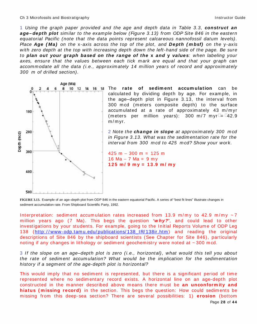
1 Using the graph paper provided and the age and depth data in Table 3.3, construct an age–depth plot similar to the example below (Figure 3.13) from ODP Site 846 in the eastern equatorial Pacific (note that the data points represent calcareous nannofossil datum levels). Place Age (Ma) on the x-axis across the top of the plot, and Depth (mbsf) on the y-axis with zero depth at the top with increasing depth down the left-hand side of the page. Be sure to plan out your graph based on the range of the x and y values: when labeling your axes, ensure that the values between each tick mark are equal and that your graph can accommodate all the data (i.e., approximately 14 million years of record and approximately 300 m of drilled section).

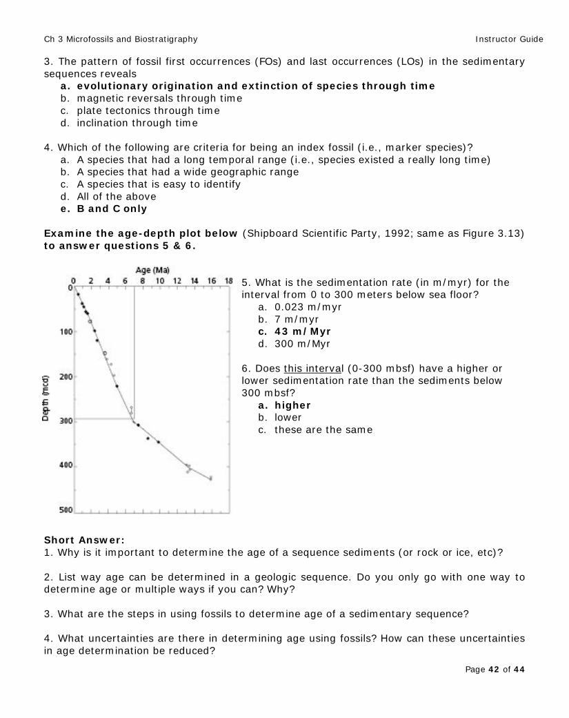
The rate of sediment accumulation can be calculated by dividing depth by age. For example, in the age–depth plot in Figure 3.13, the interval from 300 mcd (meters composite depth) to the surface accumulated at a rate of approximately 43 m/myr (meters per million years): 300 m/7 myr = 42.9 m/myr. 2 Note the change in slope at approximately 300 mcd in Figure 3.13. What was the sedimentation rate for the interval from 300 mcd to 425 mcd? Show your work. 425 m – 300 m = 125 m 16 Ma – 7 Ma = 9 my 125 m/9 my = 13.9 m/my

FIGURE 3.13. Example of an age–depth plot from ODP 846 in the eastern equatorial Pacific. A series of “best fit lines” illustrate changes in sediment accumulation rate. From Shipboard Scientific Party, 1992. Interpretation: sediment accumulation rates increased from 13.9 m/my to 42.9 m/my ~7 million years ago (7 Ma). This begs the question ‘why?’, and could lead to other investigations by your students. For example, going to the Initial Reports Volume of ODP Leg 138 (http://www-odp.tamu.edu/publications/138_IR/138ir.htm) and reading the original descriptions of Site 846 by the shipboard scientists (See Chapter for Site 846), particularly noting if any changes in lithology or sediment geochemistry were noted at ~300 mcd. 3 If the slope on an age–depth plot is zero (i.e., horizontal), what would this tell you about the rate of sediment accumulation? What would be the implication for the sedimentation history if a segment of the age-depth plot is horizontal?

This would imply that no sediment is represented, but there is a significant period of time represented where no sedimentary record exists. A horizontal line on an age-depth plot constructed in the manner described above means there must be an unconformity and hiatus (missing record) in the section. This begs the question: How could sediments be missing from this deep-sea section? There are several possibilities: 1) erosion (bottom

http://www-odp.tamu.edu/publications/138_IR/138ir.htm�


of 44

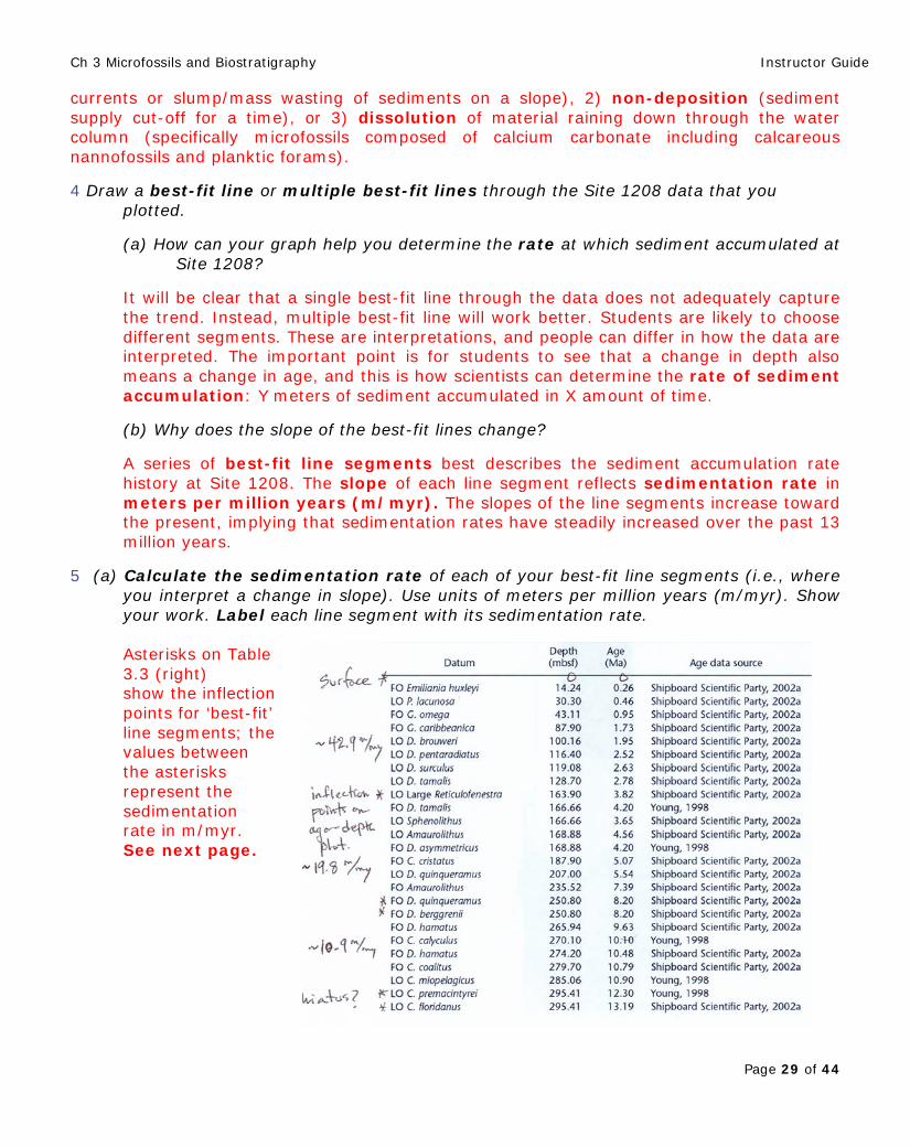
currents or slump/mass wasting of sediments on a slope), 2) non-deposition (sediment supply cut-off for a time), or 3) dissolution of material raining down through the water column (specifically microfossils composed of calcium carbonate including calcareous nannofossils and planktic forams).

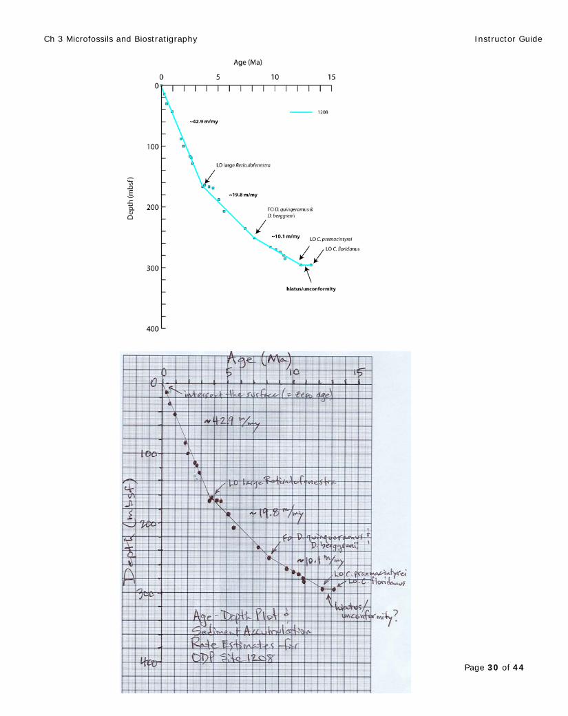
4 Draw a best-fit line or multiple best-fit lines through the Site 1208 data that you plotted.

(a) How can your graph help you determine the rate at which sediment accumulated at Site 1208?

It will be clear that a single best-fit line through the data does not adequately capture the trend. Instead, multiple best-fit line will work better. Students are likely to choose different segments. These are interpretations, and people can differ in how the data are interpreted. The important point is for students to see that a change in depth also means a change in age, and this is how scientists can determine the rate of sediment accumulation: Y meters of sediment accumulated in X amount of time.

(b) Why does the slope of the best-fit lines change?

A series of best-fit line segments best describes the sediment accumulation rate history at Site 1208. The slope of each line segment reflects sedimentation rate in meters per million years (m/myr). The slopes of the line segments increase toward the present, implying that sedimentation rates have steadily increased over the past 13 million years.

5 (a) Calculate the sedimentation rate of each of your best-fit line segments (i.e., where you interpret a change in slope). Use units of meters per million years (m/myr). Show your work. Label each line segment with its sedimentation rate.

Asterisks on Table 3.3 (right) show the inflection points for ‘best-fit’ line segments; the values between the asterisks represent the sedimentation rate in m/myr. See next page.


of 44


of 44

(b) Was the sedimentation rate constant at Site 1208 over the past 13 million years? If not, describe how the rate of sedimentation changed over time.

The sedimentation rate was not constant over the past 13 myr. Based on the best-fit line segments, it is clear that sedimentation rate at Site 1208 has increased toward the present day.

(c) Propose some hypotheses to explain these changes in sedimentation rate at this site through time. What data would you need to test these hypotheses?

Students may generate a variety of best-fit line segments. Regardless of which datums they use as inflection points in their own solution/interpretation, they should see increasing slopes toward the top of the section reflecting a steady increase in sediment accumulation rates toward the present. In the solution provided, 4 line segments are identified, including a possible unconformity/hiatus at the base of the study interval. Possible hypotheses to explain why sedimentation rates have increased since the late middle Miocene:

1. Increased terrigenous input through time (i.e., more erosion on land and increased input of mud to the ocean).

2. Increased productivity by plankton (could also be related to hypothesis 1; increased erosion on land can lead to increased availability of nutrients needed by phytoplankton).

These ideas could be tested by reading the original descriptions of Site 1208 by the shipboard scientists (http://www-odp.tamu.edu/publications/198_IR/198ir.htm; See Chapter for Site 1208 under Volume Contents; http://www-odp.tamu.edu/publications/198_IR/chap_04/chap_04.htm), particularly checking text and figures for any changes in sediment composition, sediment geochemistry, or physical properties (color reflectance, magnetic susceptibility) that may have taken place in this part of the section. From the Site 1208 chapter you can learn that there is a change in color and an increase in magnetic susceptibility in the sediments, reflecting an increase in terrigenous sediments since the Miocene. However, an increase in diatoms suggests that productivity also increased during this time. Part 3.5. How Reliable are Microfossil Datum Levels? As we observed in Part 3.3, the presence of microfossils in many types of deep-sea sediments provides a basis for age determination. The recurrent (and testable) pattern of fossil first occurrences (FOs) and last occurrences (LOs) recognized by paleontologists studying sedimentary sequences reveals the relative sequence of evolutionary origination and extinction of species through time. Because of these evolutionary events, microfossil species found in marine sediments are unique to a particular interval of geologic time making them very useful for age determination. By comparing the microfossil distribution at one site with other deep-sea sites from the same latitudinal belt (i.e., tropical-subtropical, temperate, or subpolar-polar) geoscientists can test whether the pattern or sequence of fossil first and last occurrences is consistent

http://www-odp.tamu.edu/publications/198_IR/198ir.htm�

http://www-odp.tamu.edu/publications/198_IR/chap_04/chap_04.htm�

http://www-odp.tamu.edu/publications/198_IR/chap_04/chap_04.htm�


of 44

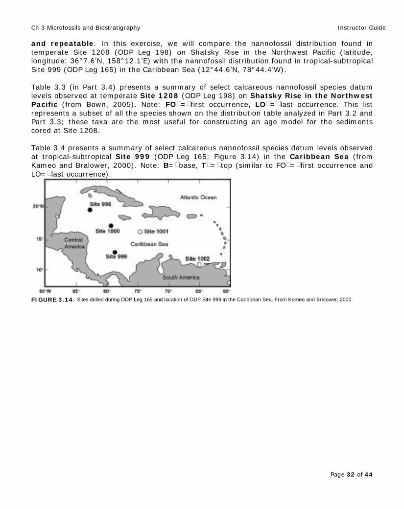
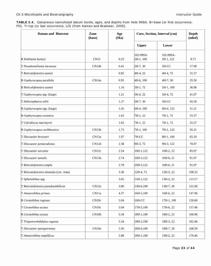
and repeatable. In this exercise, we will compare the nannofossil distribution found in temperate Site 1208 (ODP Leg 198) on Shatsky Rise in the Northwest Pacific (latitude, longitude: 36°7.6’N, 158°12.1’E) with the nannofossil distribution found in tropical-subtropical Site 999 (ODP Leg 165) in the Caribbean Sea (12°44.6’N, 78°44.4’W). Table 3.3 (in Part 3.4) presents a summary of select calcareous nannofossil species datum levels observed at temperate Site 1208 (ODP Leg 198) on Shatsky Rise in the Northwest Pacific (from Bown, 2005). Note: FO = first occurrence, LO = last occurrence. This list represents a subset of all the species shown on the distribution table analyzed in Part 3.2 and Part 3.3; these taxa are the most useful for constructing an age model for the sediments cored at Site 1208. Table 3.4 presents a summary of select calcareous nannofossil species datum levels observed at tropical-subtropical Site 999 (ODP Leg 165; Figure 3.14) in the Caribbean Sea (from Kameo and Bralower, 2000). Note: B= base, T = top (similar to FO = first occurrence and LO= last occurrence).

FIGURE 3.14. Sites drilled during ODP Leg 165 and location of ODP Site 999 in the Caribbean Sea. From Kameo and Bralower, 2000.


of 44

TABLE 3.4. Calcareous nannofossil datum levels, ages, and depths from Hole 999A; B=base (or first occurrence, FO), T=top (or last occurrence, LO) (from Kameo and Bralower, 2000).

Datum and Bioevent Zone (base)

Age (Ma)

Core, Section, Interval (cm) Depth (mbsf)

Upper Lower

B Emiliania huxleyi CN15 0.25 165-999A-2H-1, 100

165-999A-2H 1, 122 8.71

T Pseudoemiliania lacunosa CN14b 0.41 2H-7, 30 2H-CC 17.00

T Reticulofenestra asanoi 0.85 4H-4, 22 4H-4, 72 31.57

B Gephyrocapsa parallela CN14a 0.95 4H-6, 100 4H-7, 30 35.50

B Reticulofenestra asanoi 1.16 5H-1, 72 5H-1, 100 36.96

T Gephyrocapsa spp. (large) 1.21 5H-4, 22 5H-4, 72 41.07

T Helicosphaera sellii 1.27 5H-7, 30 5H-CC 45.50

B Gephyrocapsa spp. (large) 1.45 6H-4, 100 6H-4, 122 51.21

B Gephyrocapsa oceanica 1.65 7H-1, 22 7H-1, 72 55.57

T Calcidiscus macintyrei 1.65 7H-1, 22 7H-1, 72 55.57

B Gephyrocapsa caribbeanica CN13b 1.73 7H-1, 100 7H-1, 122 56.21

T Discoaster brouweri CN13a 1.97 7H-CC 8H-1, 100 65.10

T Discoaster pentaradiatus CN12d 2.38 9H-3, 72 9H-3, 122 78.07

T Discoaster surculus CN12c 2.54 10H-1,122 10H-2, 22 85.07

T Discoaster tamalis CN12b 2.74 10H-5,122 10H-6, 21 91.07

T Reticulofenestra ampla 2.78 10H-5,122 10H-6, 21 91.07

T Reticulofenestra minutula (circ. fonn) 3.36 12H-4, 72 12H-5, 22 108.32

T Sphenolithus spp. 3.65 13H-1,122 13H-2, 22 113.57

T Reticulofenestra pseudoumbilicus CN12a 3.80 13H-6,100 13H-7, 30 121.00

T Amaurolithus primus CN11a 4.37 16H-5,100 16H-6, 22 147.96

B Ceratolithus rugosus CN10c 5.04 16H-CC 17H-1, 100 150.60

T Ceratolithus acutus CN10c 5.04 17H-5,100 17H-6, 22 157.46

B Ceratolithus acutus CN10b 5.34 18H-1,100 18H-2, 22 160.96

T Triquetrorhabdulus rugosus 5.34 18H-2,100 18H-3, 22 162.46

T Discoaster quinqueramus CN10a 5.56 18H-6,100 18H-7, 30 168.50

T Amaurolithus amplificus 5.88 19H-1,100 19H-2, 22 170.46


of 44

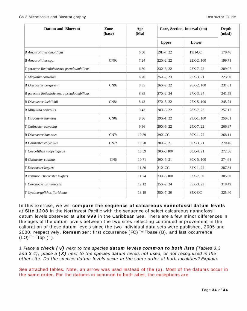
Datum and Bioevent Zone (base)

Age (Ma)

Core, Section, Interval (cm) Depth (mbsf)

Upper Lower

B Amaurolithus amplificus 6.50 19H-7, 22 19H-CC 178.46

B Amaurolithus spp. CN9b 7.24 22X-2, 22 22X-2, 100 199.71

T paracme Reticulofenestra pseudoumbilicus 6.80 23X-6, 22 23X-7, 22 209.07

T Minylitha convallis 6.70 25X-2, 23 25X-3, 21 223.90

B Discoaster berggrenii CN9a 8.35 26X-2, 22 26X-2, 100 231.61

B paracme Reticulofenestra pseudoumbilicus 8.85 27X-2, 24 27X-3, 24 241.59

B Discoaster loeblichii CN8b 8.43 27X-5, 22 27X-5, 100 245.71

B Minylitha convallis 9.43 28X-6, 22 28X-7, 22 257.17

T Discoaster hamatus CN8a 9.36 29X-1, 22 29X-1, 100 259.01

T Catinaster calyculus 9.36 29X-6, 22 29X-7, 22 266.87

B Discoaster hamatus CN7a 10.39 29X-CC 30X-1, 22 268.11

B Catinaster calyculus CN7b 10.70 30X-2, 21 30X-3, 21 270.46

T Coccolithus miopelagicus 10.39 30X-3,100 30X-4, 21 272.36

B Catinaster coalitus CN6 10.71 30X-5, 21 30X-5, 100 274.61

T Discoaster kugleri 11.50 31X-CC 32X-1, 22 287.31

B common Discoaster kugleri 11.74 33X-6,100 33X-7, 30 305.60

T Coronocyclus nitescens 12.12 35X-2, 24 35X-3, 23 318.49

T Cyclicargolithus floridanus 13.19 35X-7, 20 35X-CC 325.40

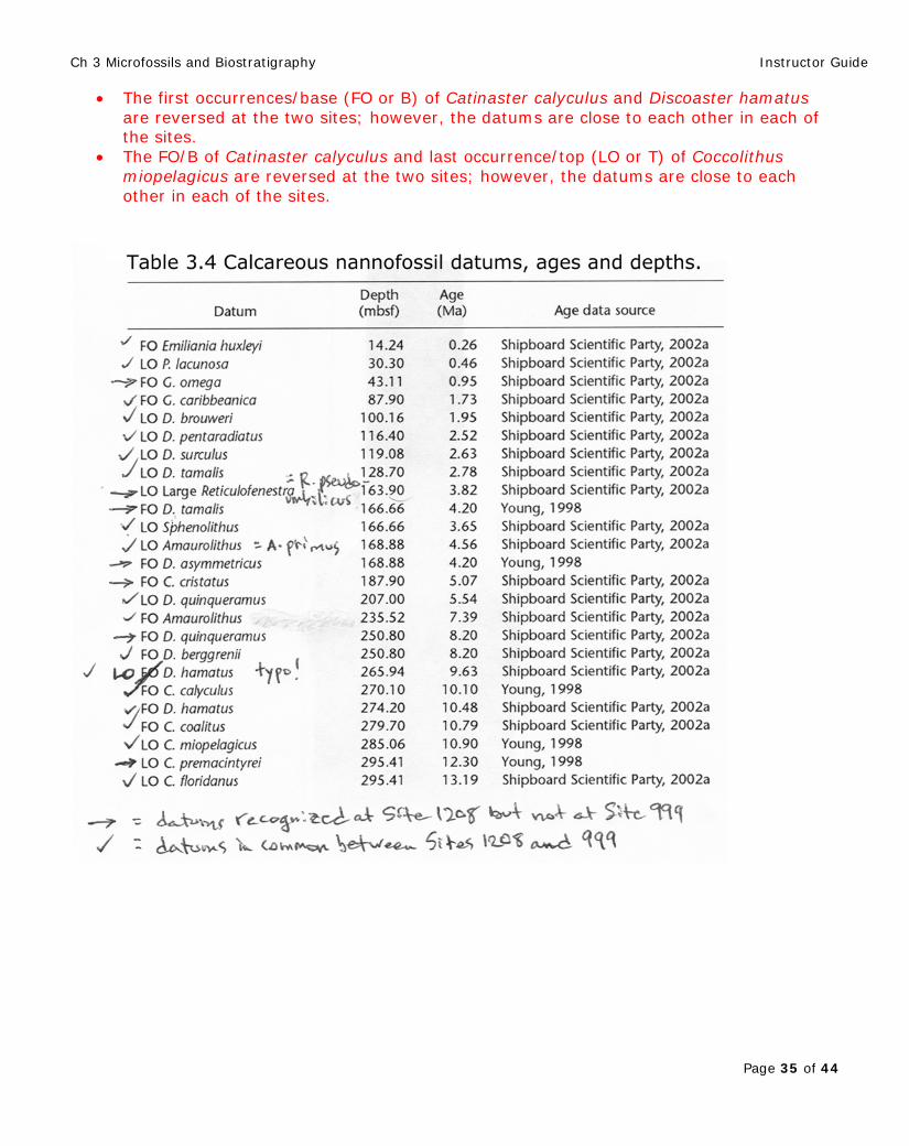
In this exercise, we will compare the sequence of calcareous nannofossil datum levels at Site 1208 in the Northwest Pacific with the sequence of select calcareous nannofossil datum levels observed at Site 999 in the Caribbean Sea. There are a few minor differences in the ages of the datum levels between the two sites reflecting continued improvement in the calibration of these datum levels since the two individual data sets were published, 2005 and 2000, respectively. Remember: first occurrence (FO) = base (B), and last occurrence (LO) = top (T). 1 Place a check (√) next to the species datum levels common to both lists (Tables 3.3 and 3.4); place a (X) next to the species datum levels not used, or not recognized in the other site. Do the species datum levels occur in the same order at both localities? Explain. See attached tables. Note, an arrow was used instead of the (x). Most of the datums occur in the same order. For the datums in common to both sites, the exceptions are:


of 44

• The first occurrences/base (FO or B) of Catinaster calyculus and Discoaster hamatus are reversed at the two sites; however, the datums are close to each other in each of the sites.

• The FO/B of Catinaster calyculus and last occurrence/top (LO or T) of Coccolithus miopelagicus are reversed at the two sites; however, the datums are close to each other in each of the sites.


of 44

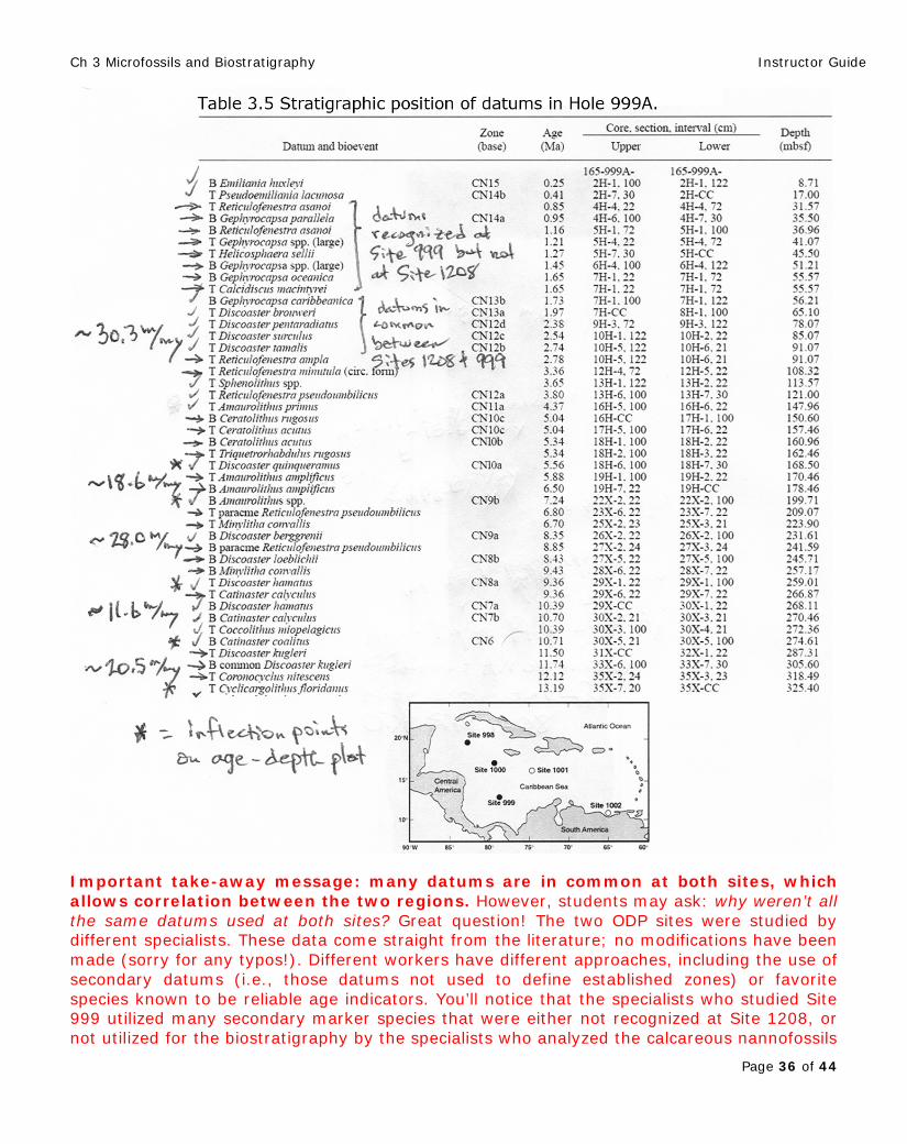
Important take-away message: many datums are in common at both sites, which allows correlation between the two regions. However, students may ask: why weren’t all the same datums used at both sites? Great question! The two ODP sites were studied by different specialists. These data come straight from the literature; no modifications have been made (sorry for any typos!). Different workers have different approaches, including the use of secondary datums (i.e., those datums not used to define established zones) or favorite species known to be reliable age indicators. You’ll notice that the specialists who studied Site 999 utilized many secondary marker species that were either not recognized at Site 1208, or not utilized for the biostratigraphy by the specialists who analyzed the calcareous nannofossils


of 44

at Site 1208. Alternatively, the Caribbean is different from the North Pacific; paleobiogeographic differences between the two regions may also explain some of the differences between the two sites. Teachable moment here about nannofossil paleoecology and paleoenvironment; tropics (Site 999 = 12°N latitude) compared with northern subtropics (Site 1208 = 36°N latitude). 2 Provide a hypothesis or two to explain the similarities and differences of the nannofossil assemblages at the two sites based on the information provided in the tables. How might you test your hypotheses?

Similarities are likely due to the rapid and widespread dispersal of calcareous nannofossils. Differences could be ascribed to environmental/ecologic differences between the two sites, which are from two different ocean basins (North Pacific and Caribbean) and different zonal belt (Site 1208 = 36°N latitude, Site 999 = 12°N latitude). These paleobiogeographic differences may have affected certain species more than others. These results could be further tested by examining the distribution of calcareous nannofossil species in other deep-sea sites. You might ask your students if they would expect to see similar results at all deep-sea sites, or only those sites from tropical-subtropical latitudes.

Comparison of Sediment Accumulation Rate Histories

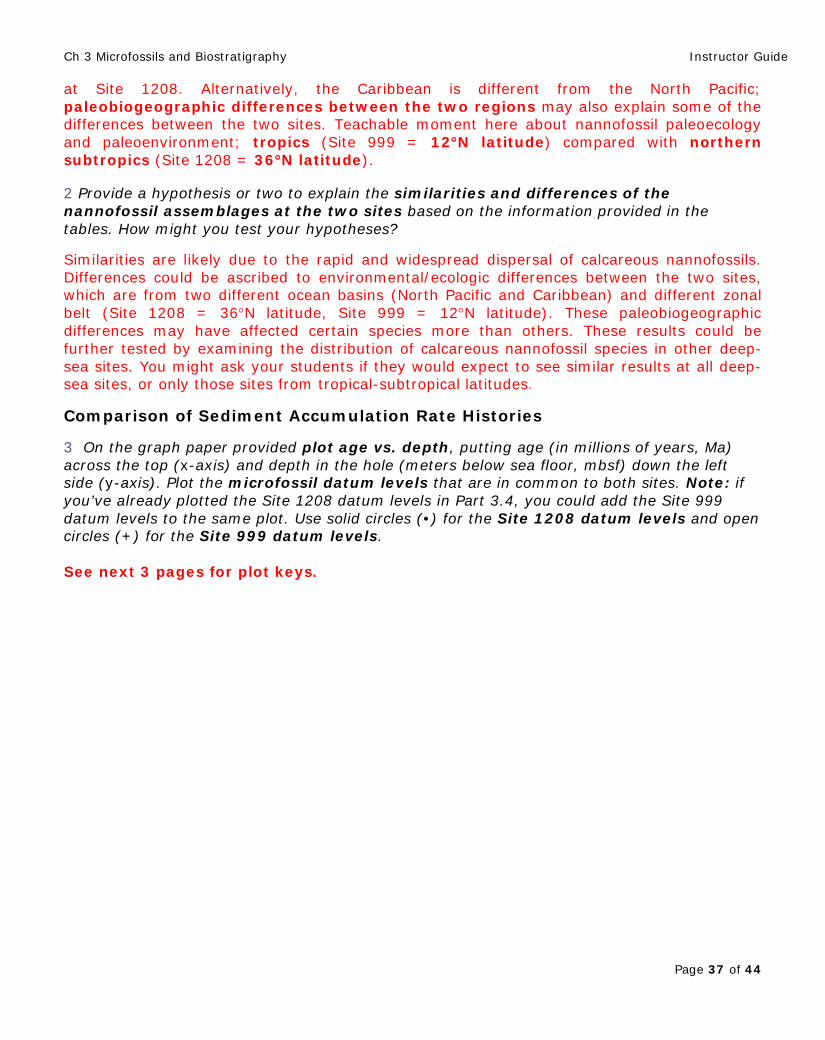
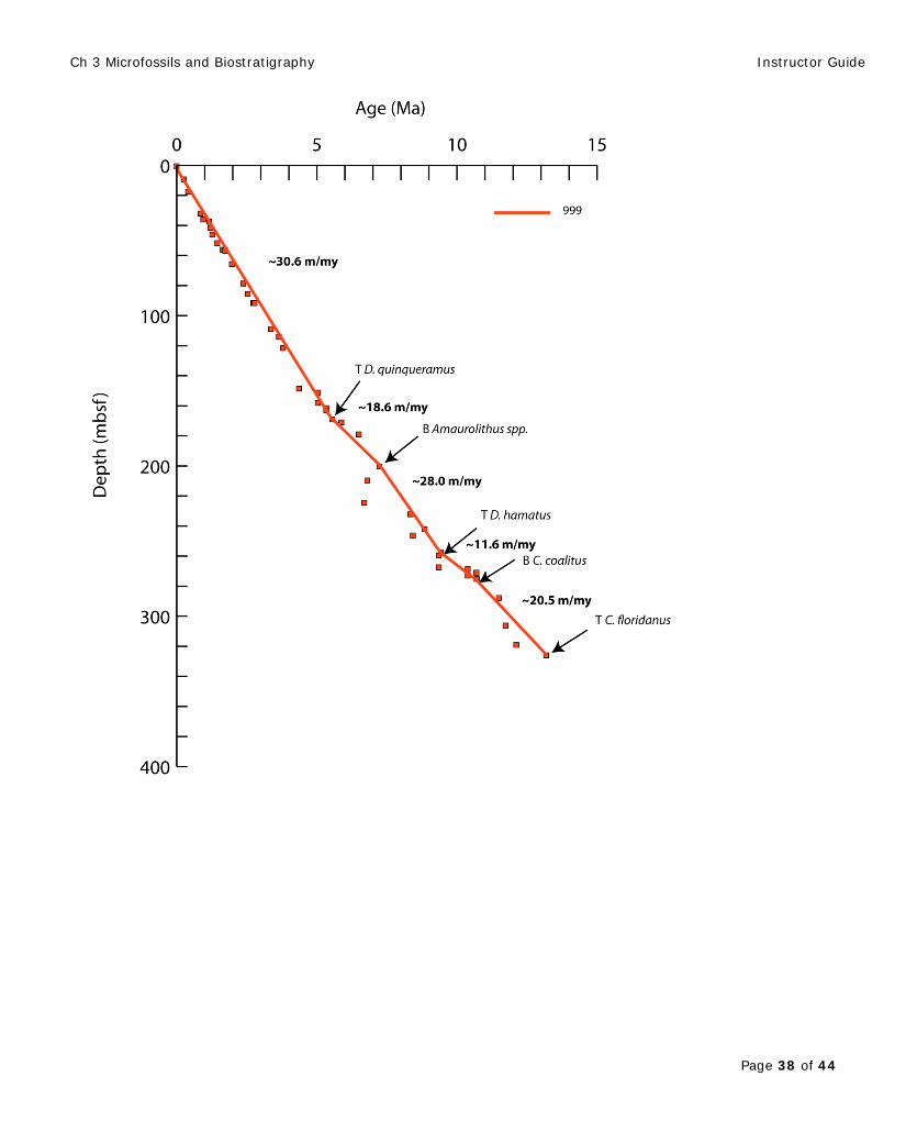
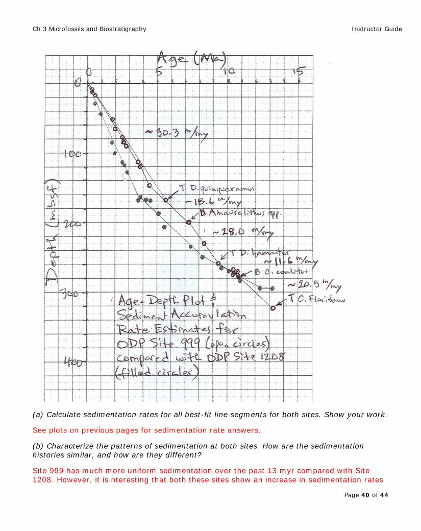
3 On the graph paper provided plot age vs. depth, putting age (in millions of years, Ma) across the top (x-axis) and depth in the hole (meters below sea floor, mbsf) down the left side (y-axis). Plot the microfossil datum levels that are in common to both sites. Note: if you’ve already plotted the Site 1208 datum levels in Part 3.4, you could add the Site 999 datum levels to the same plot. Use solid circles (•) for the Site 1208 datum levels and open circles (+) for the Site 999 datum levels. See next 3 pages for plot keys.


of 44


of 44

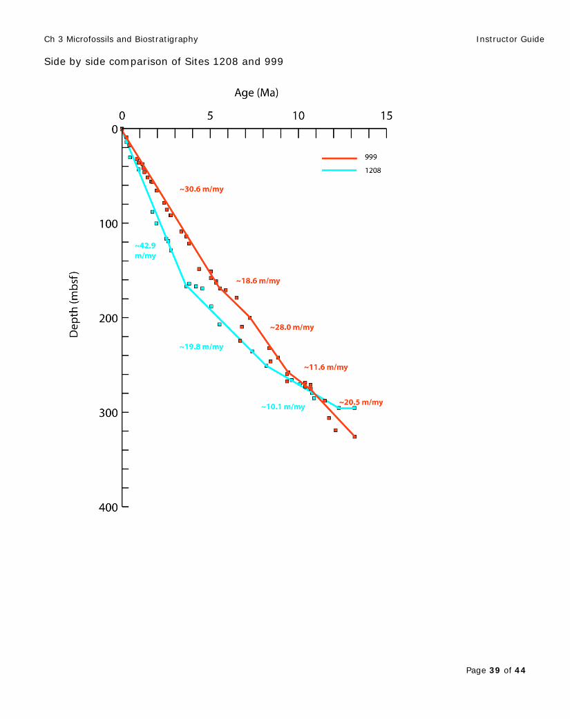
Side by side comparison of Sites 1208 and 999


of 44

(a) Calculate sedimentation rates for all best-fit line segments for both sites. Show your work.

See plots on previous pages for sedimentation rate answers.

(b) Characterize the patterns of sedimentation at both sites. How are the sedimentation histories similar, and how are they different?

Site 999 has much more uniform sedimentation over the past 13 myr compared with Site 1208. However, it is nteresting that both these sites show an increase in sedimentation rates


of 44

toward the present.

(c) Provide possible explanations for the similarities and/or differences.

As with Site 1208, there are multiple ways to interpret the changes in sedimentation rate. Site 1208 is influenced by runoff and climatic conditions in Asia (westerly winds), and by changes in productivity in the northwest Pacific. Site 999 is influenced by runoff from Central America and the emergent Andes Mountains of northern South America, as well as seasonal changes in the position of the Intertropical Convergence Zone (ITCZ). Onset of Northern Hemisphere glaciation at ~2.6 Ma may have contributed to increased meridional temperature gradients that affected everything from precipitation patterns and runoff to biological productivity. III. Summative Assessment There are several ways the instructor can assess student learning after completion of this exercise. For example, students should be able to answer the following questions after completing this exercise (note this is just a small sampling of the types of questions that could be asked): 1. You are examining the microfossils from two different sediment cores from the sea floor (see sketch below). In Core A the last occurrence of Discoaster brouweri occurs at 20 meters below sea floor. In Core B the last occurrence of Discoaster brouweri occurs at 30 meters below sea floor. Based on this information what can you conclude?

a. The layer that includes the last occurrence of D. brouweri in Core A is older. b. The layer that includes the last occurrence of D. brouweri in Core A is younger. c. The layer that includes the last occurrence of D. brouweri in Core A must be

the same age as the layer that includes the last occurrence of D. brouweri in Core B.

2. Continuing the scenario in #1, what would you do next to determine the age of this layer in core A?

a. Radiometrically-date that specific microfossil sample in your core b. Use this index fossil to determine the biozone, and therefore the fossil-based

age. c. Count the layers of sediment and they will always give you the age d. Go to a museum and find this species in an exhibit display

B A

20 m, L.O. of D. brouweri

30 m, L.O. of D. brouweri


of 44

3. The pattern of fossil first occurrences (FOs) and last occurrences (LOs) in the sedimentary sequences reveals

a. evolutionary origination and extinction of species through time b. magnetic reversals through time c. plate tectonics through time d. inclination through time

4. Which of the following are criteria for being an index fossil (i.e., marker species)?

a. A species that had a long temporal range (i.e., species existed a really long time) b. A species that had a wide geographic range c. A species that is easy to identify d. All of the above e. B and C only

Examine the age-depth plot below (Shipboard Scientific Party, 1992; same as Figure 3.13) to answer questions 5 & 6.

5. What is the sedimentation rate (in m/myr) for the interval from 0 to 300 meters below sea floor?

a. 0.023 m/myr b. 7 m/myr c. 43 m/Myr d. 300 m/Myr

6. Does this interva

a. higher

l (0-300 mbsf) have a higher or lower sedimentation rate than the sediments below 300 mbsf?

b. lower c. these are the same

Short Answer: 1. Why is it important to determine the age of a sequence sediments (or rock or ice, etc)? 2. List way age can be determined in a geologic sequence. Do you only go with one way to determine age or multiple ways if you can? Why? 3. What are the steps in using fossils to determine age of a sedimentary sequence? 4. What uncertainties are there in determining age using fossils? How can these uncertainties in age determination be reduced?


of 44

5. If we compared two sedimentary sequences from two different locations and found that they contain the same biozone boundary (e.g., top of CN 14a), are the layers from these two different sequences the same age? Explain. Are they necessarily the depth? Explain. 6. What are biozones? How are the biozones in a new location (e.g., like the case study we did from the NW Pacific) determined? 7. What are First Occurrences (FO) and last Occurrences (LO)? Be able to find FO and LO for given species in table to define biozones. [Remember FO is also Base and LO is also Top.] 8. How might you explain an older species being above a younger species in your sedimentary sequence? [note: this is not the norm, older should be deeper (below) younger, so what could mix this up?] IV. Supplemental Materials

• To download a poster of microfossils made by teachers for teachers go to: http://joidesresolution.org/node/265

• For a short video taken on the JOIDES Resolution showing how core samples are taken and processed for foraminifera biostratigraphy go to: http://www.nisd.net/jay/joides/index.htm then selected “Processing core samples & observing micro fossils with Dr. Leckie (video)” or go to: http://www.schooltube.com/video/a4ca5da84f1145a7d1e6/

• The Microfossil Image Recovery and Circulation for Learning and Education ("MIRACLE") website has a wealth of images and descriptions of the main microfossil groups: http://www.ucl.ac.uk/GeolSci/micropal/welcome.html. It includes descriptions of the history, classification, applications, biology, lifestyle, preparation techniques, and observation techniques of foraminifera, calcareous nannofossils, diatoms, radiolarians, conodonts, ostrocods, and dinoflagellates. It also contains many links to academic and professional organization sites that focus on micropaleontology.

V. References

Bown, P.R., 2005, Cenozoic calcareous nannofossil biostratigraphy, ODP Leg 198 Site 1208 (Shatsky Rise, Northwest Pacific Ocean). Proceedings of the Ocean Drilling Program, Scientific Results, Bralower, T.J., et al. (eds), vol. 198, College Station, TX, Ocean Drilling Program, pp. 1–44. http://www-odp.tamu.edu/publications/198_SR/104/104.htm

Gradstein, F., 1987, Report of the Second Conference on Scientific Ocean Drilling (Cosod II), European Science Foundation, Strasbourg, France, p. 109.

Kameo, K. and Bralower, T.J., 2000, Neogene calcareous nannofossil biostratigraphy of Sites 998, 999, and 1000, Caribbean Sea. In Proceedings of the Ocean Drilling Program, Scientific Results, vol. 165, Leckie, R.M., et al. (eds), College Station, TX, Ocean Drilling Program, pp. 3–17. http://www-odp.tamu.edu/publications/165_SR/chap_01/chap_01.htm

Katz, M.E., et al., 2005, Biological overprint of the geological carbon cycle. Marine Geology, 217, 323–38.

http://joidesresolution.org/node/265�

http://www.nisd.net/jay/joides/index.htm�

http://www.schooltube.com/video/a4ca5da84f1145a7d1e6/�

http://www.ucl.ac.uk/GeolSci/micropal/welcome.html�

http://www-odp.tamu.edu/publications/198_SR/104/104.htm�

http://www-odp.tamu.edu/publications/165_SR/chap_01/chap_01.htm�


of 44

Shipboard Scientific Party, 1992, Site 846. In Initial Reports of the Ocean Drilling Program, vol. 138, Mayer, L., et al., College Station, TX, Ocean Drilling Program, pp. 256–333; doi:10.2973/odp.proc.ir.138.111.1992.http://www-odp.tamu.edu/publications/138_IR/VOLUME/CHAPTERS/ir138_11.pdf

Shipboard Scientific Party, 2002, Explanatory notes. In Proceedings ODP, Initial Reports of the Ocean Drilling Program, vol. 198, Bralower, T.J., et al., College Station, TX, Ocean Drilling Program, pp. 1–63. doi:10.2973/odp.proc.ir.198.102.2002. http://www-odp.tamu.edu/publications/198_IR/198TOC.HTM

Young, J.R., 1998, Neogene. In Calcareous Nannofossil Biostratigraphy, Bown, P.R. (ed.), Kluwer Academic Publishers, Dordrecht, The Netherlands, pp. 225–65.

http://www-odp.tamu.edu/publications/138_IR/VOLUME/CHAPTERS/ir138_11.pdf�

http://www-odp.tamu.edu/publications/138_IR/VOLUME/CHAPTERS/ir138_11.pdf�

http://www-odp.tamu.edu/publications/198_IR/198TOC.HTM�

http://www-odp.tamu.edu/publications/198_IR/198TOC.HTM�

instructor guide chapter 3 microfossils and biostra tigraphy · 2017-10-20 · chapter 3....

Documents