innovation, technological interdependence, and …...innovation, technological interdependence, and...
TRANSCRIPT
Innovation, Technological Interdependence, and
Economic Growth˚
Douglas HanleyUniversity of Pittsburgh
January 15, 2015
Abstract
There is substantial heterogeneity across industries in the level of interdependence be-
tween new and old technologies. I propose a measure of this interdependence–an index
of sequentiality in innovation–which is the transfer rate of patents in a particular indus-
try. I find that highly sequential industries have higher profitability, higher variance of
firm growth, lower exit rates, and lower rates of patent expiry. To better understand these
trends, I construct a model of firm dynamics where the productivity of firms evolves en-
dogenously through innovations. New innovators either replace existing technologies or
must purchase the rights to existing technologies from incumbents in order to produce,
depending on the level of sequentiality in the industry. Estimating the model using data
on US firms and recent data on US patent transfers, I can account for a large fraction of
the cross-industry trends described above. Because innovation results in larger monopoly
distortions in more sequential industries, there is an overinvestment of research inputs
into these industries. This misallocation, which amounts to 2.5% in consumption equiv-
alent terms, can be partially remedied using a patent policy featuring weaker protection
in more sequential industries, producing welfare gains of 1.7%.
JEL classification: L11, O31, O33, O34, O38
Keywords: Innovation, firm dynamics, technological change, optimal policy.
˚I am deeply indebted to my advisor Ufuk Akcigit for his guidance and support. Additionally, I would like
to thank Dirk Krueger and Iourii Manovskii for their valuable advice. I am also grateful to Daron Acemoglu,
William Kerr, and Nicolas Serrano-Velarde for their help in the research process. I received numerous useful
comments and suggestions from seminar participants in the University of Pennsylvania Macro Club, Money
Macro Workshop, and Growth Reading Group.
2 Hanley Innovation, Technological Interdependence, and Economic Growth
1 Introduction
The innovation process is known to be highly cumulative. New ideas are created because in-
ventors “stand on the shoulders of giants” that preceded them. However, the extent to which
new technology is dependent upon old technology varies substantially from field to field. In
some areas, such as pharmaceuticals, new technologies often replace existing ones, render-
ing them obsolete. Here creative destruction is a natural byproduct of innovation. In other
areas, such as computer software, new technologies complement existing ones and are inte-
grated with them into a final product. In this setting, technologies are generated incremen-
tally, potentially across multiple firms and over long periods of time, necessitating some form
of technology transfer between firms.
Motivated by this last consideration, I proxy the level of technological interdependence in
an industry by the rate of patent transfer between firms, which, following the literature, I refer
to as sequentiality. Using this index of sequentiality, I find that more sequential industries
have higher profitability, higher variance of firm growth, lower exit rates, and lower rates of
patent expiry1. These trends may at first seem puzzling, but as I will show, they in fact arise
naturally from a model of firm-driven technological progress featuring heterogeneity across
industries in the level of sequentiality. By studying such a model and constraining it with data,
we can address a number of important questions. For instance, how does the appropriability
of the returns to innovation vary with sequentiality? Does cross-industry heterogeneity in
sequentiality produce substantial research misallocation? And finally, what role can patent
policy play in this setting?
Estimating this model using firm-level data on patenting and balance sheet information,
each of the trends noted above is matched qualitatively, and a large fraction of the variation
is accounted for quantitatively. I show theoretically that the larger the sequentiality in a par-
ticular industry, the more severe the monopoly distortions induced by a particular level of
innovation. This leads to an overallocation of research inputs into more sequential indus-
tries. In line with this result, I find that implementing an optimal industry dependent patent
policy, which features weaker patent protection in more sequential industries, can remedy a
substantial fraction of this misallocation, over and above an optimal uniform patent policy.
This paper contributes to the existing body of literature along both empirical and theoret-
ical dimensions. First, regarding theory, I construct a parsimonious, micro-founded model of
1Patent holders must pay maintenance fees at 4, 8, and 12 years after granting or face permanent expiry.
3 Hanley Innovation, Technological Interdependence, and Economic Growth
sequential innovation and endogenous technological change that formalizes the process by
which new ideas are generated, built upon, and subsequently transferred between firms or
rendered obsolete. Sequential innovation has already been given treatment in the literature
on innovation and endogenous growth, notably in Green and Scotchmer (1995) and Bessen
and Maskin (2009), as well as Hopenhayn, Llobet, and Mitchell (2006), who analyze the in-
herent trade-off present between rewarding incumbents and subsequent innovators that will
replace them. This model captures the same trade-off while incorporating features of more
empirically focused models of firm dynamics such as those of Klette and Kortum (2004) and
Lentz and Mortensen (2008).2 I characterize the innovation decisions of firms in a manner that
provides intuition for the various economic forces at play and solve for a variety of observable
quantities.
In the model, new innovations have differing degrees of dependence on existing technol-
ogy. High levels of dependence (sequential innovations) necessitate some form of patent sales
agreement between the owners of existing technology and new innovators.3 Conversely, low
levels of dependence (independent innovations) necessitate little adjudication of rights be-
tween firms as the new innovation simply renders the old one obsolete, leading to the expi-
ration of the original patent. Laitner and Stolyarov (2013) entertain a similar distinction in a
model of exogenous innovation. In my model, innovation is endogenously determined and
the frequency of sequential innovation varies from industry to industry.
As has been done in Akcigit and Kerr (2010) and Atkeson and Burstein (2010), firms can
engage in two types of innovation: external, where they innovate on product lines owned by
other firms, and internal, where they innovate on their own product lines. The effect of se-
quentiality on the rate of external innovation is ex ante ambiguous due to the presence of two
countervailing forces. First, the value of owning an existing product line is larger in more se-
quential industries as they feature lower rates of creative destruction from competitors and
larger streams of payments from subsequent sequential innovators who buy their patents.
However, because of the increased probability of sequential innovation, which necessitates a
payout to the existing incumbent, the net effect on innovators will be ambiguous. This stands
2These in turn build upon foundational works such as Romer (1990), Aghion and Howitt (1992), and Grossman
and Helpman (1991), as well as numerous other works produced in the interim. See Aghion et al. (2013) for a very
recent survey.3I assume that firms always sell their patents rather than licensing them. In the model, this will always be the
optimal type of agreement due to monopolistic distortions.
4 Hanley Innovation, Technological Interdependence, and Economic Growth
in contrast to the model presented in Akcigit, Celik, and Greenwood (2013), which features
the positive effect of revenues from patent sales, but not the inhibition of follow on innovation
due to continuing patent protection. In the case of internal innovation, the picture becomes
clearer, as only the positive effect described above remains.
Broadly speaking, the sequentiality dimension introduced here fills a gap between two
classes of models commonly studied in the endogenous growth literature. That is, most mod-
els either feature firms that face no threat of replacement from other innovators at the product
line level, as in the expanding variety model of Romer (1990), or just the opposite, that firms
innovate solely on other firms’ product lines and can take over production at will upon a suc-
cessful innovation, as in Aghion and Howitt (1992), Grossman and Helpman (1991), or Klette
and Kortum (2004). The model presented in this paper will act as a bridge between the two
extremes presented above. In the extreme of full sequentiality, much of the gains from inno-
vation will be internalized through repeated selling of patent rights down the quality ladder,
though distortions from bargaining will complicate this process slightly. In contrast to the
Romer model, however, this will come at the cost of a buildup of monopoly power. In the
extreme of no sequentiality, we find ourselves with a standard model of creative destruction.
The second contribution of this paper is to enrich our understanding of the data on patent-
ing and innovation by firms. To study cross-industry differences in the sequentiality of inno-
vation, I propose a method of classifying technology classes–an index of sequentiality–based
upon the fraction of patents that are transferred in their lifetime. Looking back to the intro-
ductory examples, patents in the major pharmaceutical patent classes are transferred 15% of
the time, while the same figure for telecommunications is twice as large at 30%. Using this
ordering, I document a variety of trends in both the patent data and in linked firm-level data.
One would naturally expect the level of sequentiality in a particular industry to have an ef-
fect upon innovations dynamics in that industry. For instance, highly sequential industries
should feature lower rates of patent obsolescence, as patents are more likely to be built upon
and integrated into a larger portfolio rather than being replaced by a new type of technology.
This buildup of larger patent portfolios should in turn cause profits to rise, as leading firms
will have a larger technological lead over their nearest competitor.
In the data description section below, I document that these trends are in fact present in
the data, and I enumerate other trends observed in the cross-industry data, namely that more
sequential industries feature lower exit rates and higher variance in firm growth. The former
is a natural implication of the reduction in the rate of creative destruction in more sequential
5 Hanley Innovation, Technological Interdependence, and Economic Growth
industries. The latter effect arises from interaction with firm heterogeneity. Higher sequen-
tiality and the concomitant patent transfers result in the agglomeration of more productive
control into the hands of high quality firms. This magnifies the persistent growth differences
between firms of differing quality, resulting in more volatile firm growth overall, particularly
over longer time periods.
In addition to cross-industry statistics, there are notable trends occurring at the firm and
patent level. There is a strong tendency for patents to flow from older and larger firms to
younger and smaller firms, with the age dimension showing a distinctly stronger trend than
the size dimension. This echoes the finding of Figueroa and Serrano (2013) that small firms
receive a disproportionate amount of patent transfers.4 These facts, in conjunction with the
cross-industry trend in firm growth volatility lend support to the notion that patent transfers
reflect an underlying process of reallocation amongst firms. This is particularly compelling
given the strong evidence that younger, smaller firms excel in many measures of firm perfor-
mance such as growth and profitability (both in the data presented here and in other works
such as Akcigit and Kerr (2010) and Acemoglu et al. (2013)).
The third contribution of this paper is to estimate the proposed model using data on public
firms and patents in the US, provide a detailed quantitative analysis of the results, and study
the implications for optimal patent policy. I use a Simulated Method of Moments (SMM) es-
timator to match various features of the US data on patent grants, transfers, and expiry and
on firm level growth rates and profitability. The patent data comes from the USPTO/Google
database and includes data on filings, grants, expiry, and transfers. Data on patent transfers in
particular has not been utilized extensively in the literature, especially in a structural setting.
The patent data is aggregated to the firm level and matched to Compustat balance sheet data
using sophisticated name matching routines.
The estimated model is able to match the targeted moments quite well. In addition, the
model can match various non-targeted features of the data, including some of the major trends
noted above. The resulting eight-year patent expiration rate over all industries is 39%, com-
pared to 34% in the data, while the standard deviation is 15% compared to 13% in the data.
Thus the model captures the proportional variation in the data, while slightly overshooting
the magnitude. Other cross-industry trends, such as the relationship between transfer rates
and profitability, firm growth variance, and exit rate are qualitatively captured, and the model
is able to quantitatively account for a large fraction of these tends.
4They use firm size information (greater or less than 500 employees) contained in patent renewal applications.
6 Hanley Innovation, Technological Interdependence, and Economic Growth
As predicted by theory, the level of internal innovation rises with sequentiality, with a 52%
increase moving from the least to most sequential industry. The level of external innovation,
whose dependence on sequentiality was theoretically ambiguous, falls modestly along this
dimension, largely due to bargaining distortions that limit the appropriability of back-loaded
profit streams. To assess potential misallocation of production and research labor, both within
and between industries, I consider a constrained social planner who can choose innovation
rates but is still subject to monopoly distortions induced by patenting. I show theoretically
that the larger the sequentiality in a particular industry, the more severe the monopoly dis-
tortions induced by an increase in innovation rates. Thus for either type of innovation, the
planner optimally choses a profile that falls sharply with sequentiality–in the case of external
innovation, much more so than in the equilibrium–so as to limit the monopoly distortions
caused by the buildup of large, protected technological leads by firms. The equilibrium yields
a consumption equivalent welfare 2.5% lower than that of the constrained social planner.
Finally, I investigate the implications of the model for patent policy. I consider both a uni-
form patent policy and one that depends upon the sequentiality of the industry in question.
For the purposes of implementation, the sequentiality of a particular industry can be inferred
using the monotonic relationship between sequentiality and the patent transfer rate in the
equilibrium of the estimated model. The above discussion of the social planner’s optimum
leads one to suspect that the optimal patent policy would feature weaker protection in more
sequential industries. Indeed, I find that for certain very low levels of sequentiality, an infi-
nite patent is called for. The optimal patent length then decreases from infinity to a minimal
value of 6 years in the most sequential industry. This policy results in welfare gains of 1.7% in
consumption equivalent terms. For comparison, the optimal constant patent policy calls for
a mean patent length of 12 years and delivers welfare gains of only 0.9%.
The remainder of the paper is laid out as follows: in Section 2, I describe the data set used
and enumerate the notable trends in the data; in Section 3, I construct a model capable of
matching these facts and describe its equilibrium properties; in Section 4, I describe the es-
timation procedure and results; in Section 5, I provide a detailed quantitative analysis of the
estimated model with accompanying decompositions and policy experiments; and finally in
Section 6, I conclude the analysis.
7 Hanley Innovation, Technological Interdependence, and Economic Growth
2 Empirical Findings
Data on patent grants, expirations, and transfers was acquired from the USPTO Bulk Down-
load site (hosted by Google). Firm names are matched and aggregated into persistent entities
based on a name matching algorithm described in Appendix A.5
For each patent transfer, the following information is provided: (1) the name of the ori-
gin firm and destination firm (assignor and assignee), (2) the date that the patent was legally
transferred, (3) the date that the transfer was recorded by the patent office, and (4) the pur-
pose of the transfer, amongst other things. In particular, the information on the purpose of
the transfer (known as the conveyance text) is used to filter out mergers, licensing agreements,
and collateralizations, leaving only simple patent sales, which account for about 85% of the
original data points.
The names of the origin and destination firm were matched to the set of entities produced
from the patent grant data using the same name matching algorithms. In order to focus on
innovating firms and not firms that are simply acquiring patents for other reasons (such as
resale), I keep only transfers to firms that have already acquired patents through filing and
granting. This eliminates firms that act solely as patent brokers. Furthermore, to exclude
instances where conglomerates are transferring patents amongst their constituent units, I
eliminate transfers where the origin and destination firm names are sufficiently close, using
a more aggressive version of the original name matching algorithm (this is also described in
Appendix A).
To enrich the data on patent grants, I also use data on the payment of patent maintenance
fees. Firms must pay fees to the US patent office after 4, 8, and 12 years from the time of
granting. If these fees are not paid, the patent expires permanently. If a patent is maintained
through the initial 12 year period, it remains valid until 20 years from its filing date.6 This data
thus gives discretized information on the active lifespan of a patent. In total, 35% of patents
expire after 8 years, while 48% make it to the natural expiry date. Using the data on patent
expiration gives us fairly direct information on the rate of patent obsolescence and hence a
window into the level of product market competition faced by firms. Using this in conjunction
5Python code to parse, match, and aggregate the USPTO patent data (along with Compustat data) can be
found at https://github.com/iamlemec/patents.6Traditionally, the maximum patent length was 17 years from the grant date. The 1994 Uruguay Round Agree-
ments Act changed this to the above criterion. See Graham and Vishnubhakat (2013) for a review of the relevant
statutes.
8 Hanley Innovation, Technological Interdependence, and Economic Growth
with the data on patent transfers helps us understand the importance of sequential innovation
and its impact on firm dynamics and the incentives to innovate.
To register a patent reassignment with the USPTO, a firm must pay a one-time $40 flat fee.
The bulk of the cost is likely to be found in simply filling out the paperwork. Firms already
incur legal fees to arrange the contracts for the transfer deals, so going the extra step to reg-
ister with the patent office is probably not a huge effort. Patent maintenance fees are slightly
higher but still not large compared to the common estimates of patent value in the literature.
Some studies, such as Pakes (1986), Pakes and Schankerman (1984), and Bessen and Meurer
(2008), have used patent renewal patterns to estimate the distribution of patent valuations. A
survey by Griliches (1998) reports that various studies found a highly skewed distribution of
patent valuations, with mean valuation estimates in the hundreds of thousands of current US
dollars, and an obsolescence rate of between 10% and 20% per year. The fees required for re-
newal at 4, 8, and 12 years are $1600, $3600, and $7200, respectively. These fees are cut in half
for small entities (less than 500 employees), and halved again for “micro entities” (targeted
towards individual inventors). This self-reported size information provides useful data on the
actual size of particular patenting firms. Figueroa and Serrano (2013) utilize this to study the
relationship between firm size and patent transferring activity.
An important consideration is the possibility that firms license the patents of other firms
rather than buying them outright. Firms are required to register patent sales or transfers in
order to retain patent rights for a particular technology. However, there is no such requirement
for patent licensing, which is regulated by state law in the US.7 Approximately 1% of patent
transfer entries list licensing as the documented activity, though this cannot be guaranteed
to be a complete record. Looking across industries, there is no systematic variation in this
fraction of reported licensing activity.
2.1 Major Trends
Testing various cross-industry predictions necessitates dividing the sample of patents and
firms into particular industry level categories. For this exercise, I employ the level one tech-
nology class utilized by the US patent office. There are 714 such classes represented in the full
patent grant dataset, with a median size of around one thousand patents. Using the first-level
classification provides sufficient granularity to capture the specific features of various tech-
7See Dykeman and Kopko (2004) for an overview of the relevant statutes and case law.
9 Hanley Innovation, Technological Interdependence, and Economic Growth
nological fields while being large enough to avoid excessive noise in aggregate statistics due
to small within-industry samples.
It is also possible to extend patent classification information to the firm level. By assigning
to a firm the modal patent class amongst its portfolio of patents, we can look at how various
firm characteristics vary with technological field. Though most firms have patents in multiple
patent classes, the modal patent class accounts for an average of 50% of a firm’s patents. This
extension to firm characteristics will be important for analyzing trends in balance sheet data
from Compustat. For patent data, much of the analysis can be done purely on the patent
level. However, I do analyze the patent data using firm-level class assignment for robustness
and find similar results.
Industry level regressions are done using weighted least squares. The weighting used is
simply the size of the particular technology class in terms of total patents granted. Data on
patenting is available from 1976 to the present. For the facts below, I look at the five-year pe-
riod from 1995 to 2000. This allows sufficient lead time to have realistic values for firm patent
stocks, which is the count of patents that are unexpired at any given time. In a steady state
world, a lead in time equal to or greater than the patent length suffices. Additionally, it allows
sufficient lag time to analyze future transfer, maintenance, and citation activity. The correla-
tions presented below are also weighted by patent class size. In each of the figures accompa-
nying the following facts, the point size represents the total number of patents granted (the
weight) and the color represents the the numerical patent class, which ranges from 1 (lightest)
to 800 (darkest). Because patent classes have been added incrementally over time, the patent
class (color) also provides a very good proxy for how recently the patent class was created.
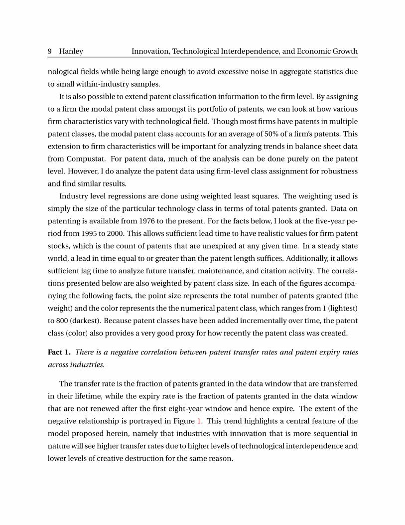
Fact 1. There is a negative correlation between patent transfer rates and patent expiry rates
across industries.
The transfer rate is the fraction of patents granted in the data window that are transferred
in their lifetime, while the expiry rate is the fraction of patents granted in the data window
that are not renewed after the first eight-year window and hence expire. The extent of the
negative relationship is portrayed in Figure 1. This trend highlights a central feature of the
model proposed herein, namely that industries with innovation that is more sequential in
nature will see higher transfer rates due to higher levels of technological interdependence and
lower levels of creative destruction for the same reason.
10 Hanley Innovation, Technological Interdependence, and Economic Growth
FIGURE 1: TRANSFER–EXPIRY RELATIONSHIP
Relationship between patent transfer and expiry. Red line: WLS regression β “´0.33.
Correlation is ρ“´0.34.
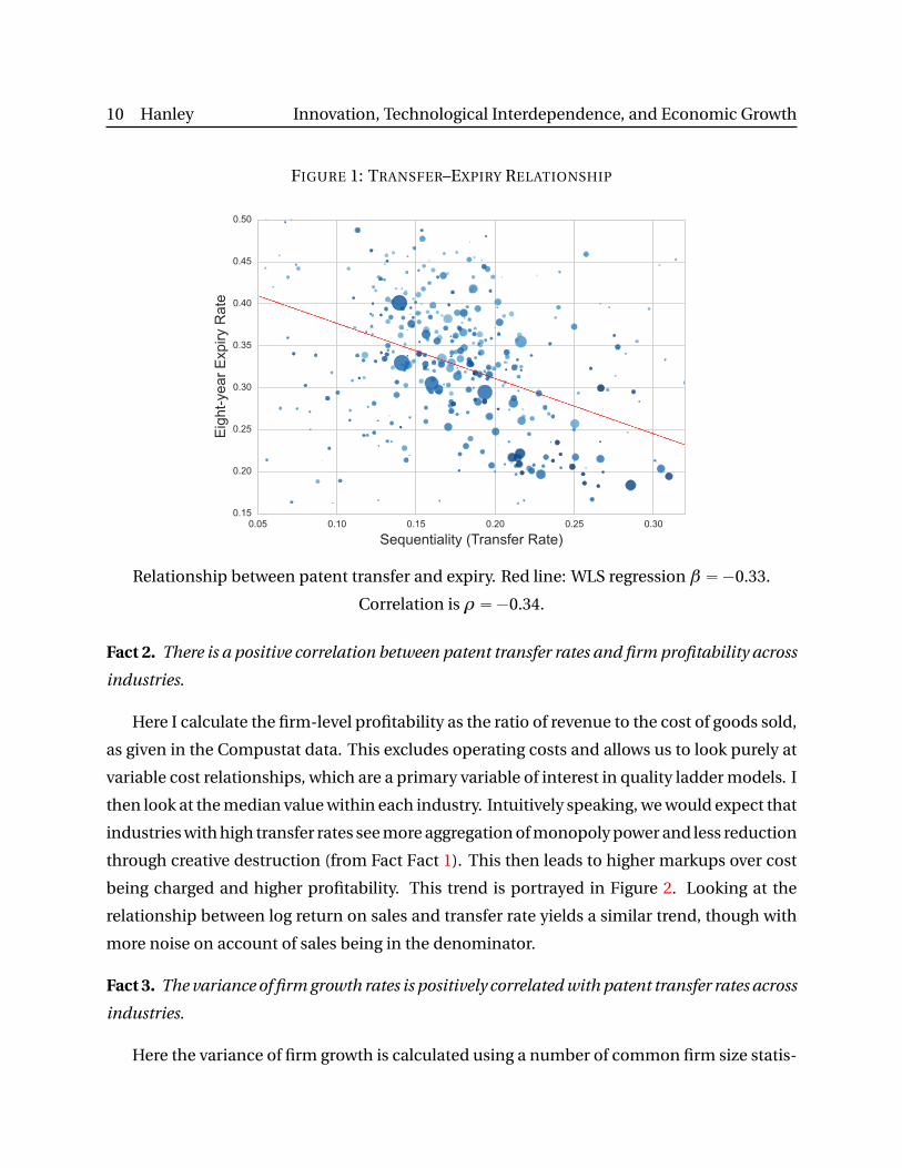
Fact 2. There is a positive correlation between patent transfer rates and firm profitability across
industries.
Here I calculate the firm-level profitability as the ratio of revenue to the cost of goods sold,
as given in the Compustat data. This excludes operating costs and allows us to look purely at
variable cost relationships, which are a primary variable of interest in quality ladder models. I
then look at the median value within each industry. Intuitively speaking, we would expect that
industries with high transfer rates see more aggregation of monopoly power and less reduction
through creative destruction (from Fact Fact 1). This then leads to higher markups over cost
being charged and higher profitability. This trend is portrayed in Figure 2. Looking at the
relationship between log return on sales and transfer rate yields a similar trend, though with
more noise on account of sales being in the denominator.
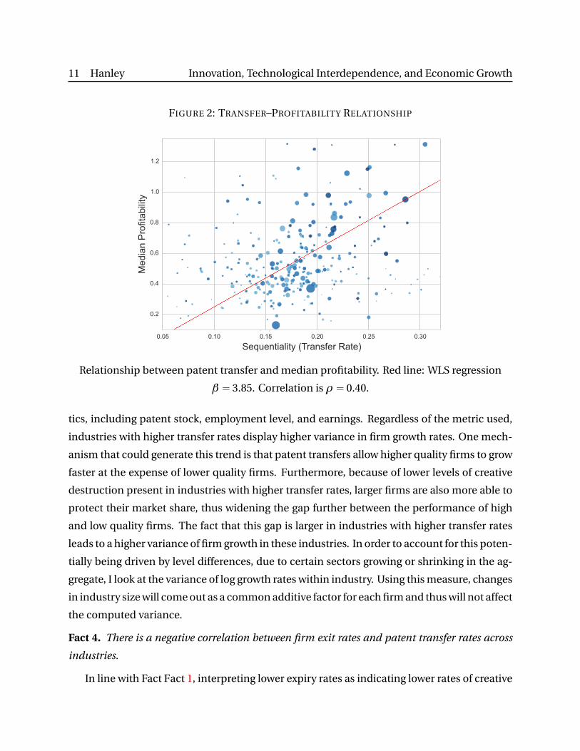
Fact 3. The variance of firm growth rates is positively correlated with patent transfer rates across
industries.
Here the variance of firm growth is calculated using a number of common firm size statis-
11 Hanley Innovation, Technological Interdependence, and Economic Growth
FIGURE 2: TRANSFER–PROFITABILITY RELATIONSHIP
Relationship between patent transfer and median profitability. Red line: WLS regression
β “ 3.85. Correlation is ρ“ 0.40.
tics, including patent stock, employment level, and earnings. Regardless of the metric used,
industries with higher transfer rates display higher variance in firm growth rates. One mech-
anism that could generate this trend is that patent transfers allow higher quality firms to grow
faster at the expense of lower quality firms. Furthermore, because of lower levels of creative
destruction present in industries with higher transfer rates, larger firms are also more able to
protect their market share, thus widening the gap further between the performance of high
and low quality firms. The fact that this gap is larger in industries with higher transfer rates
leads to a higher variance of firm growth in these industries. In order to account for this poten-
tially being driven by level differences, due to certain sectors growing or shrinking in the ag-
gregate, I look at the variance of log growth rates within industry. Using this measure, changes
in industry size will come out as a common additive factor for each firm and thus will not affect
the computed variance.
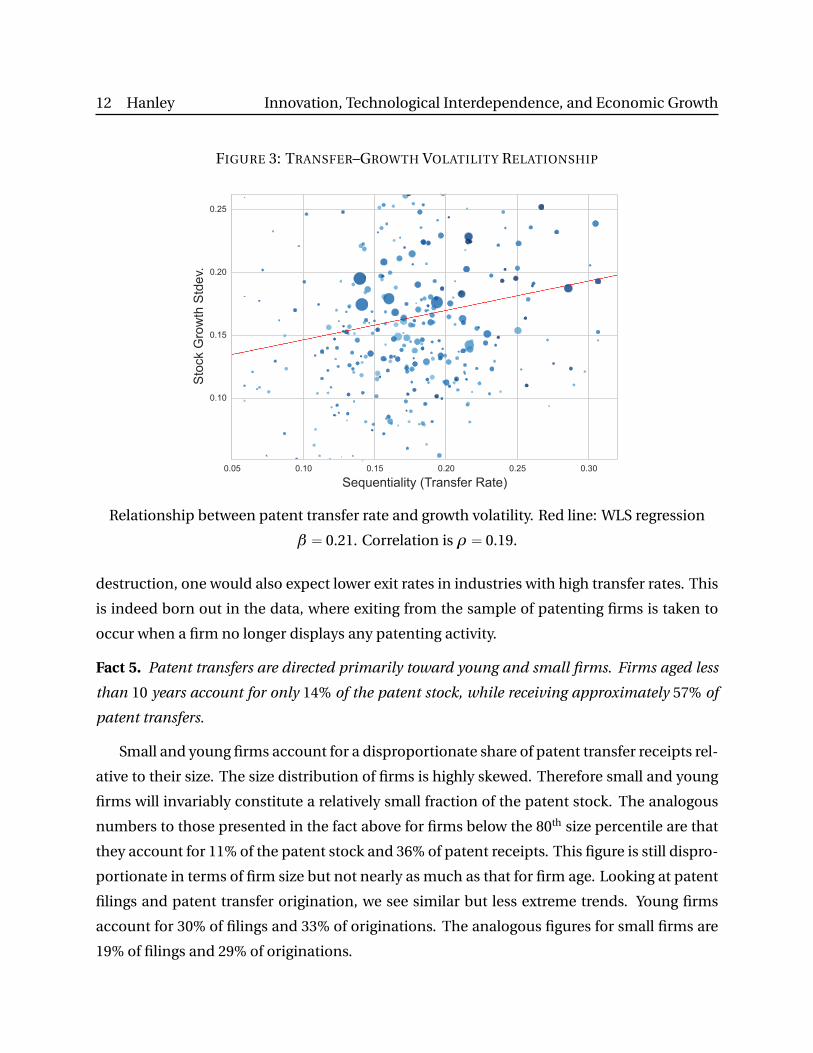
Fact 4. There is a negative correlation between firm exit rates and patent transfer rates across
industries.
In line with Fact Fact 1, interpreting lower expiry rates as indicating lower rates of creative
12 Hanley Innovation, Technological Interdependence, and Economic Growth
FIGURE 3: TRANSFER–GROWTH VOLATILITY RELATIONSHIP
Relationship between patent transfer rate and growth volatility. Red line: WLS regression
β “ 0.21. Correlation is ρ“ 0.19.
destruction, one would also expect lower exit rates in industries with high transfer rates. This
is indeed born out in the data, where exiting from the sample of patenting firms is taken to
occur when a firm no longer displays any patenting activity.
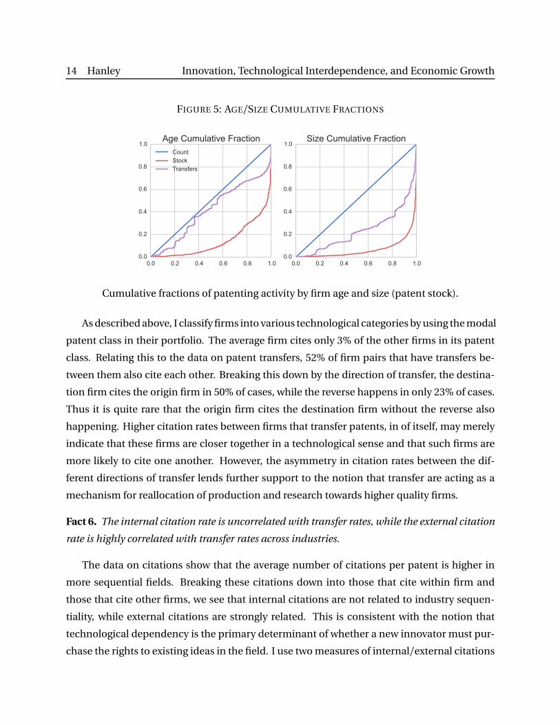
Fact 5. Patent transfers are directed primarily toward young and small firms. Firms aged less
than 10 years account for only 14% of the patent stock, while receiving approximately 57% of
patent transfers.
Small and young firms account for a disproportionate share of patent transfer receipts rel-
ative to their size. The size distribution of firms is highly skewed. Therefore small and young
firms will invariably constitute a relatively small fraction of the patent stock. The analogous
numbers to those presented in the fact above for firms below the 80th size percentile are that
they account for 11% of the patent stock and 36% of patent receipts. This figure is still dispro-
portionate in terms of firm size but not nearly as much as that for firm age. Looking at patent
filings and patent transfer origination, we see similar but less extreme trends. Young firms
account for 30% of filings and 33% of originations. The analogous figures for small firms are
19% of filings and 29% of originations.
13 Hanley Innovation, Technological Interdependence, and Economic Growth
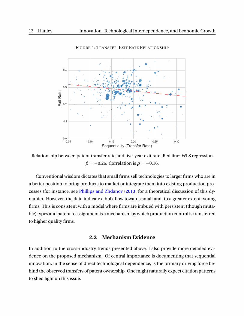
FIGURE 4: TRANSFER–EXIT RATE RELATIONSHIP
Relationship between patent transfer rate and five-year exit rate. Red line: WLS regression
β “´0.26. Correlation is ρ“´0.16.
Conventional wisdom dictates that small firms sell technologies to larger firms who are in
a better position to bring products to market or integrate them into existing production pro-
cesses (for instance, see Phillips and Zhdanov (2013) for a theoretical discussion of this dy-
namic). However, the data indicate a bulk flow towards small and, to a greater extent, young
firms. This is consistent with a model where firms are imbued with persistent (though muta-
ble) types and patent reassignment is a mechanism by which production control is transferred
to higher quality firms.
2.2 Mechanism Evidence
In addition to the cross-industry trends presented above, I also provide more detailed evi-
dence on the proposed mechanism. Of central importance is documenting that sequential
innovation, in the sense of direct technological dependence, is the primary driving force be-
hind the observed transfers of patent ownership. One might naturally expect citation patterns
to shed light on this issue.
14 Hanley Innovation, Technological Interdependence, and Economic Growth
FIGURE 5: AGE/SIZE CUMULATIVE FRACTIONS
Cumulative fractions of patenting activity by firm age and size (patent stock).
As described above, I classify firms into various technological categories by using the modal
patent class in their portfolio. The average firm cites only 3% of the other firms in its patent
class. Relating this to the data on patent transfers, 52% of firm pairs that have transfers be-
tween them also cite each other. Breaking this down by the direction of transfer, the destina-
tion firm cites the origin firm in 50% of cases, while the reverse happens in only 23% of cases.
Thus it is quite rare that the origin firm cites the destination firm without the reverse also
happening. Higher citation rates between firms that transfer patents, in of itself, may merely
indicate that these firms are closer together in a technological sense and that such firms are
more likely to cite one another. However, the asymmetry in citation rates between the dif-
ferent directions of transfer lends further support to the notion that transfer are acting as a
mechanism for reallocation of production and research towards higher quality firms.
Fact 6. The internal citation rate is uncorrelated with transfer rates, while the external citation
rate is highly correlated with transfer rates across industries.
The data on citations show that the average number of citations per patent is higher in
more sequential fields. Breaking these citations down into those that cite within firm and
those that cite other firms, we see that internal citations are not related to industry sequen-
tiality, while external citations are strongly related. This is consistent with the notion that
technological dependency is the primary determinant of whether a new innovator must pur-
chase the rights to existing ideas in the field. I use two measures of internal/external citations
15 Hanley Innovation, Technological Interdependence, and Economic Growth
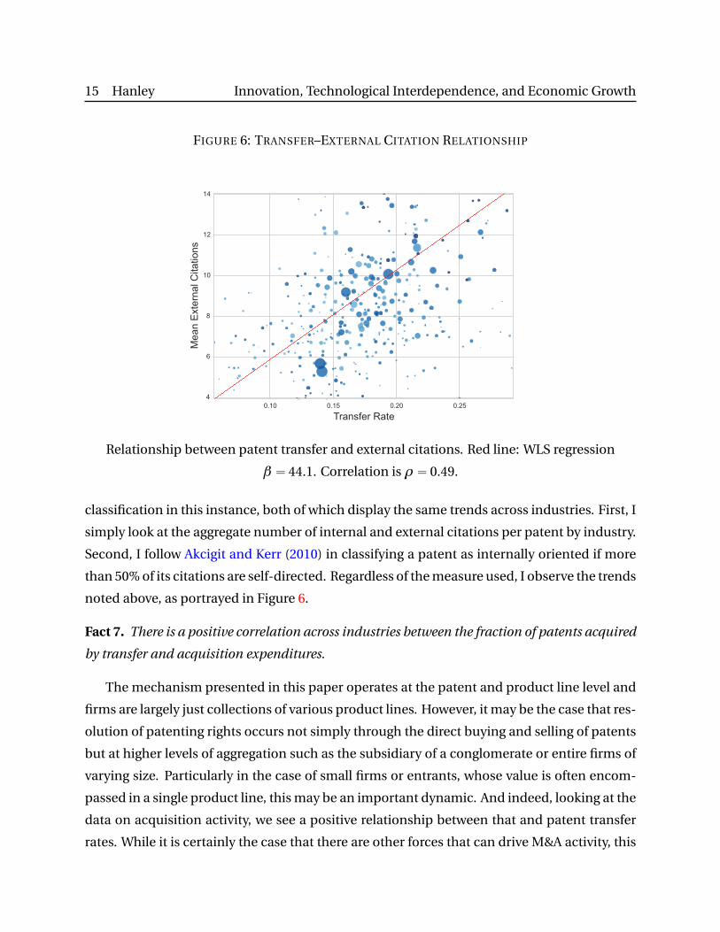
FIGURE 6: TRANSFER–EXTERNAL CITATION RELATIONSHIP
Relationship between patent transfer and external citations. Red line: WLS regression
β “ 44.1. Correlation is ρ“ 0.49.
classification in this instance, both of which display the same trends across industries. First, I
simply look at the aggregate number of internal and external citations per patent by industry.
Second, I follow Akcigit and Kerr (2010) in classifying a patent as internally oriented if more
than 50% of its citations are self-directed. Regardless of the measure used, I observe the trends
noted above, as portrayed in Figure 6.
Fact 7. There is a positive correlation across industries between the fraction of patents acquired
by transfer and acquisition expenditures.
The mechanism presented in this paper operates at the patent and product line level and
firms are largely just collections of various product lines. However, it may be the case that res-
olution of patenting rights occurs not simply through the direct buying and selling of patents
but at higher levels of aggregation such as the subsidiary of a conglomerate or entire firms of
varying size. Particularly in the case of small firms or entrants, whose value is often encom-
passed in a single product line, this may be an important dynamic. And indeed, looking at the
data on acquisition activity, we see a positive relationship between that and patent transfer
rates. While it is certainly the case that there are other forces that can drive M&A activity, this
16 Hanley Innovation, Technological Interdependence, and Economic Growth
trend indicates that the technological landscape plays an important role. Discussion of how
this data may be mapped into the model is deferred until the section on estimation.
3 Model
In this section, I present a continuous-time model of firm dynamics and endogenous techno-
logical growth. After specifying the various elements of the model, I characterize the dynamic
equilibrium. I then focus on the case of the steady state, with the objective of producing pre-
dictions that map into the trends described in the previous section.
3.1 Consumers
There is a unit mass of immortal consumer-workers in the economy. Each has one unit of
labor that they supply inelastically. Their utility is a function on the infinite flow stream of
consumption starting at time t “ 0. In particular, they discount the future at rate δ and have
an instantaneous utility function of upc q with constant relative risk aversion parameter σ.
Thus their utility function can be expressed as
U pc q “
ż 8
0
„
c pt q1´σ´1
1´σ
expp´δt qd t
where c is a consumption profile that specifies the level of consumption at each point in time.
All agents earn a wage w from employment. They also have access to a risk-free bond paying
interest r and having zero net supply in the aggregate. Let their bond holding profile be the
function a . Their budget equation is then given by
c ` 9a “w ` r a
where time dependence is suppressed for notational convenience. There is a single final good
Y for consumption, which is normalized to have a unit price at each point in time. Because all
costs are purely in terms of labor, the final good resource constraint for the economy is simply
c “ Y . The associated Euler equation for this problem the delivers the result
g ”9Y
Y“
9c
c“
r ´δ
σ
Letting the common growth rate of Y and c be denoted by g , we arrive at r “δ`σg .
17 Hanley Innovation, Technological Interdependence, and Economic Growth
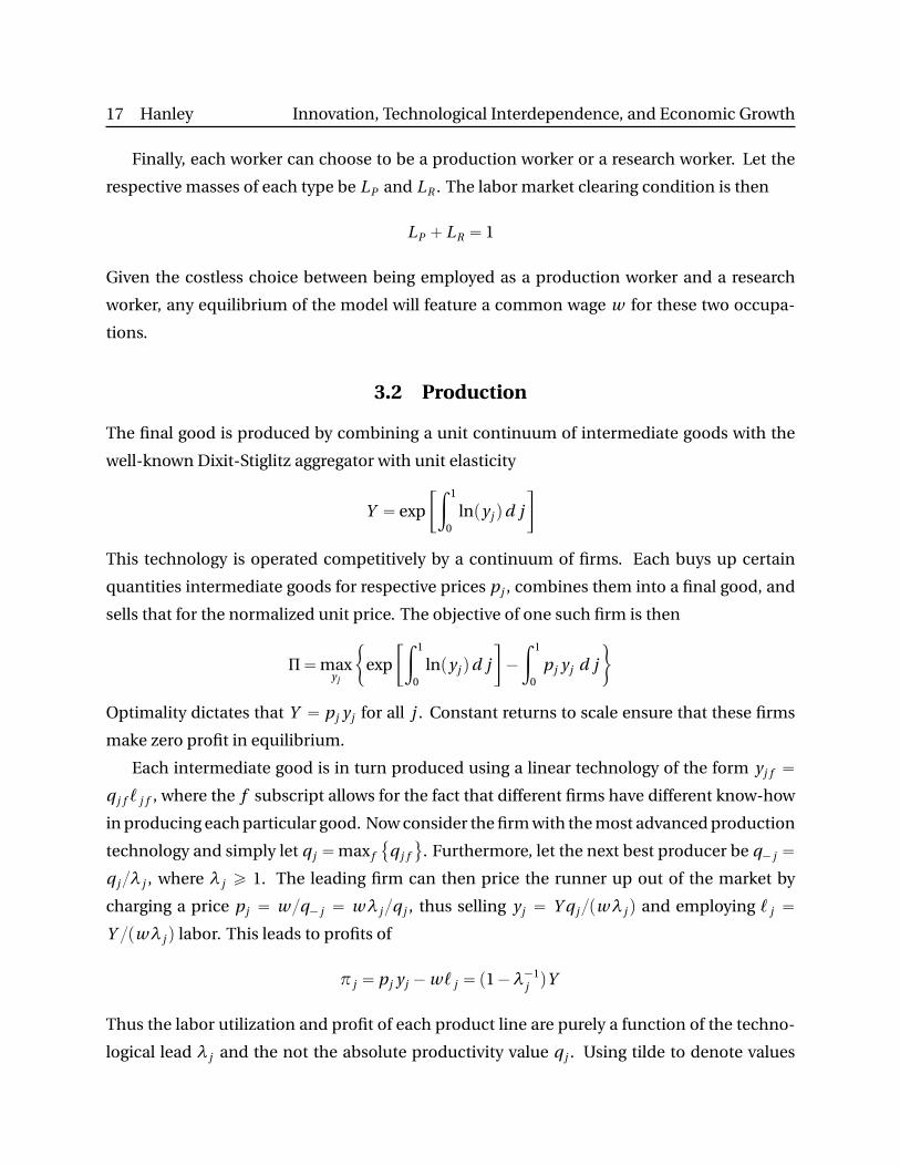
Finally, each worker can choose to be a production worker or a research worker. Let the
respective masses of each type be LP and LR . The labor market clearing condition is then
LP ` LR “ 1
Given the costless choice between being employed as a production worker and a research
worker, any equilibrium of the model will feature a common wage w for these two occupa-
tions.
3.2 Production
The final good is produced by combining a unit continuum of intermediate goods with the
well-known Dixit-Stiglitz aggregator with unit elasticity
Y “ exp
„ż 1
0lnpyj qd j
This technology is operated competitively by a continuum of firms. Each buys up certain
quantities intermediate goods for respective prices pj , combines them into a final good, and
sells that for the normalized unit price. The objective of one such firm is then
Π“maxyj
"
exp
„ż 1
0lnpyj qd j
´
ż 1
0pj yj d j
*
Optimality dictates that Y “ pj yj for all j . Constant returns to scale ensure that these firms
make zero profit in equilibrium.
Each intermediate good is in turn produced using a linear technology of the form yj f “
q j f ` j f , where the f subscript allows for the fact that different firms have different know-how
in producing each particular good. Now consider the firm with the most advanced production
technology and simply let q j “max f
q j f
(
. Furthermore, let the next best producer be q´ j “
q j λ j , where λ j ě 1. The leading firm can then price the runner up out of the market by
charging a price pj “ w q´ j “ wλ j q j , thus selling yj “ Y q j pwλ j q and employing ` j “
Y pwλ j q labor. This leads to profits of
π j “ pj yj ´w ` j “ p1´λ´1j qY
Thus the labor utilization and profit of each product line are purely a function of the techno-
logical lead λ j and the not the absolute productivity value q j . Using tilde to denote values
18 Hanley Innovation, Technological Interdependence, and Economic Growth
normalized by Y , the labor utilization and profit for a product line with technological lead λ
are given by
`pλq “λ´1
rwand rπpλq “ 1´λ´1
Having fully characterized the production decisions of intermediate goods producing firms,
we can now use these production values to address the innovations decisions of firms.
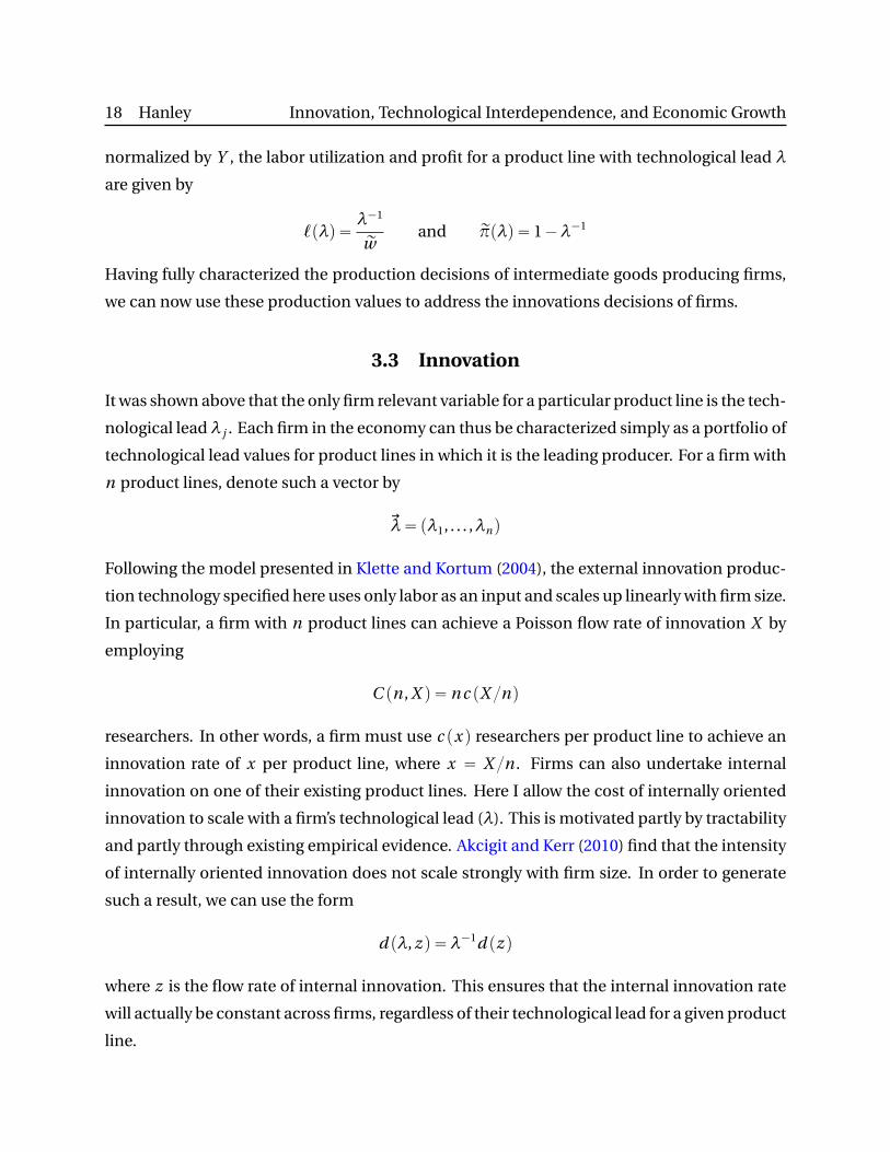
3.3 Innovation
It was shown above that the only firm relevant variable for a particular product line is the tech-
nological lead λ j . Each firm in the economy can thus be characterized simply as a portfolio of
technological lead values for product lines in which it is the leading producer. For a firm with
n product lines, denote such a vector by
~λ“ pλ1, . . . ,λnq
Following the model presented in Klette and Kortum (2004), the external innovation produc-
tion technology specified here uses only labor as an input and scales up linearly with firm size.
In particular, a firm with n product lines can achieve a Poisson flow rate of innovation X by
employing
C pn , X q “ n c pX nq
researchers. In other words, a firm must use c px q researchers per product line to achieve an
innovation rate of x per product line, where x “ X n . Firms can also undertake internal
innovation on one of their existing product lines. Here I allow the cost of internally oriented
innovation to scale with a firm’s technological lead (λ). This is motivated partly by tractability
and partly through existing empirical evidence. Akcigit and Kerr (2010) find that the intensity
of internally oriented innovation does not scale strongly with firm size. In order to generate
such a result, we can use the form
d pλ, z q “λ´1d pz q
where z is the flow rate of internal innovation. This ensures that the internal innovation rate
will actually be constant across firms, regardless of their technological lead for a given product
line.
19 Hanley Innovation, Technological Interdependence, and Economic Growth
The functional forms given allow one to treat each firm simply as a collection of research
labs, each associated with a particular product line. Denote the value of a research lab with
technological lead λ by V pλq. A firm with portfolio ~λwill then have value
V p~λq “8ÿ
i“1
V pλi q
A research lab will accrue profits from production and generate innovations. Successful in-
novations will garner new research labs with their associated production and innovation ca-
pabilities. Now we can characterize all firm decisions by addressing the problem at a product
line level.
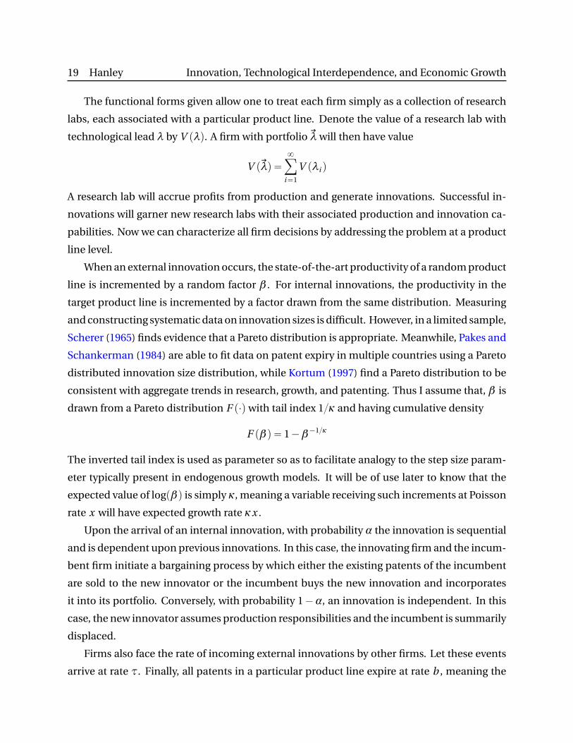
When an external innovation occurs, the state-of-the-art productivity of a random product
line is incremented by a random factor β . For internal innovations, the productivity in the
target product line is incremented by a factor drawn from the same distribution. Measuring
and constructing systematic data on innovation sizes is difficult. However, in a limited sample,
Scherer (1965) finds evidence that a Pareto distribution is appropriate. Meanwhile, Pakes and
Schankerman (1984) are able to fit data on patent expiry in multiple countries using a Pareto
distributed innovation size distribution, while Kortum (1997) find a Pareto distribution to be
consistent with aggregate trends in research, growth, and patenting. Thus I assume that, β is
drawn from a Pareto distribution F p¨qwith tail index 1κ and having cumulative density
F pβq “ 1´β´1κ
The inverted tail index is used as parameter so as to facilitate analogy to the step size param-
eter typically present in endogenous growth models. It will be of use later to know that the
expected value of logpβq is simply κ, meaning a variable receiving such increments at Poisson
rate x will have expected growth rate κx .
Upon the arrival of an internal innovation, with probability α the innovation is sequential
and is dependent upon previous innovations. In this case, the innovating firm and the incum-
bent firm initiate a bargaining process by which either the existing patents of the incumbent
are sold to the new innovator or the incumbent buys the new innovation and incorporates
it into its portfolio. Conversely, with probability 1´α, an innovation is independent. In this
case, the new innovator assumes production responsibilities and the incumbent is summarily
displaced.
Firms also face the rate of incoming external innovations by other firms. Let these events
arrive at rate τ. Finally, all patents in a particular product line expire at rate b , meaning the
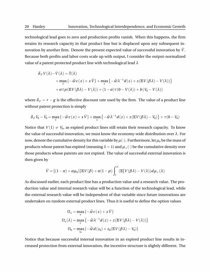
20 Hanley Innovation, Technological Interdependence, and Economic Growth
technological lead goes to zero and production profits vanish. When this happens, the firm
retains its research capacity in that product line but is displaced upon any subsequent in-
novation by another firm. Denote the present expected value of successful innovation by sV .
Because both profits and labor costs scale up with output, I consider the output-normalized
value of a patent protected product line with technological lead λ
δF V pλq´ 9V pλq “ rπpλq
`maxxt´ rw c px q` x sV u`max
z
´ rwλ´1d pz q` z pEV pβλq´V pλqq(
`ατp pEV pβλq´V pλqq`p1´αqτp0´V pλqq` b pV0´V pλqq
where δF “ r ´ g is the effective discount rate used by the firm. The value of a product line
without patent protection is simply
δF V0´9V0“max
xt´ rw c px q` x sV u`max
z
´ rwλ´1d pz q` z pEV pβλq´V0q(
`τp0´V0q
Notice that V p1q ‰ V0, as expired product lines still retain their research capacity. To know
the value of successful innovation, we must know the economy-wide distribution over λ. For
now, denote the cumulative density for this variable byµp¨q. Furthermore, letµ0 be the mass of
products whose patent has expired (meaning λ“ 1) and µ`p¨q be the cumulative density over
those products whose patents are not expired. The value of successful external innovation is
then given by
sV “ rp1´αq`αµ0qsEV pβq`αp1´p q
ż 8
1pErV pβλq´V pλqqdµ`pλq
As discussed earlier, each product line has a production value and a research value. The pro-
duction value and internal research value will be a function of the technological lead, while
the external research value will be independent of that variable since future innovations are
undertaken on random external product lines. Thus it is useful to define the option values
Ωx “maxxt´ rw c px q` x sV u
Ωz pλq “maxz
´ rwλ´1d pz q` z pEV pβλq´V pλqq(
Ω0“maxz0
t´ rw d pz0q` z0pEV pβλq´V0qu
Notice that because successful internal innovation in an expired product line results in in-
creased protection from external innovation, the incentive structure is slightly different. The
21 Hanley Innovation, Technological Interdependence, and Economic Growth
product line value function expressions can then be simplified to
pδF `p1´αqτqV pλq´ 9V pλq “πpλq`Ωx `Ωz pλq`ατp pEV pβλq´V pλqq` b pV0´V pλqq
pδF `τqV0´9V0“Ωx `Ω0
Having characterized the firm value functions and their dynamics, we must also address the
evolution of the state space, which in this case consists of the technological lead distributions.
First, the respective masses of expired and unexpired product lines will satisfy the flow equa-
tions
9µ0“ bµ`´pτ` z0qµ0 and 9µ`“ pτ` z0qµ0´ bµ`
Focusing on unexpired product lines (where λą 0), the distribution will satisfy the flow equa-
tion
9µ`pλq “pb `p1´αqτqrF pλq´µ`pλqs´ pατ` z q
ż 8
1r1´ F pλλ1qsdµ`pλ
1q (1)
`
ˆ
9µ`µ`
˙
rF pλq´µ`pλqs (2)
The first two terms are what we would expect in the case without patent expiry. Independent
innovations arrive at rate p1´αqτ and reset the technological lead to some random value β ,
and similarly for patent expiry b . Meanwhile, sequential and internal innovations arrive at
rate ατ` y and increment the technological lead by some random value β . The last term
simply deals with the fact that there are also product lines flowing into and out of expiry.
3.4 Equilibrium
Having described the optimization problems faced by consumers and firms, we can now move
on to characterizing their optimal behavior and setting forth conditions for aggregate consis-
tency given the equilibrium variables we have introduced. The aggregate information needed
by the firm to make decisions includes the rate of creative destruction τ, the wage rate w , and
the interest rate r . Finally, the firm needs to know the state space, namely the distribution
over technological leads, which is fully described by the respective masses of expired and un-
expired product lines µ0 and µ` and the distribution of technological leads over unexpired
product lines µ`p¨q. Eventually, it will be shown that the mean inverse over µ`p¨q
Γ`“
ż 8
0λ´1dµ`pλq
22 Hanley Innovation, Technological Interdependence, and Economic Growth
will suffice for the purposes of the firm and for aggregate consistency. Now posit a linearly
separable ansatz for the unexpired product line value function
V pλq “ A´Bλ´1
Recall that rπpλq “ 1´λ´1. Inserting the above into the product line value function and equat-
ing coefficients on the constant term and the λ´1 terms yields the following characterization
of the coefficients
pδF ` b `p1´αqτqA´ 9A“ 1`Ωx ` b V0
pδF ` b `p1´αqτqB ´ 9B “ 1´Ωz ´ατp Bp1`κ´1q
HereΩx is the option value of external innovation. Because of the concavity of the profit func-
tion in the technological lead, the gross returns to internal innovation are decreasing. How-
ever, since the the cost also decreases by the same proportion, the net returns also scale down
with the technological lead. Thus internal innovation shows up in the variable portion of the
value function as
Ωz “maxz
´ rw d pz q` z Bp1`κ´1q(
Ω0“maxz0
t´ rw d pz0q` z0pA´Bp1`κq´V0qu
with Ωz pλq “λ´1Ωz . Using these expressions, the expected gain from innovation can be sim-
plified to
sV “ pp1´αq`αµ0qpA´Bp1`κqq`αp1´p qµ`Γ`Bp1`κ´1q
The labor market clearing condition will include contributions from production, external in-
novation (from incumbents and entrants) and internal innovation (on expired and unexpired
product lines) as delineated below
1“Γ
rw`p1` e qc px q`µ0d pz0q`µ`Γ`d pz q (3)
where Γ is the average inverse technological lead over all product lines and satisfies Γ “ µ0`
µ`Γ`. The flow equation for Γ` is described in the next section and depends only on µ0, µ`,
and Γ` itself. Therefore, with regards to solving the equilibrium by determining the evolution
of the state space, Γ` is a sufficient statistic forµ`p¨q. In fact, justµ0 and Γ would be a sufficient
state space. However, the three variable specification proves to be notationally cleaner.
23 Hanley Innovation, Technological Interdependence, and Economic Growth
Aggregate consistency of the rate of external innovation requires thatτ“ p1`e qx . Though
it is not necessary for the equilibrium solution, the growth rate will naturally be of interest
as an implication of this model. Each innovation, regardless of whether it is sequential or
independent furthers the state of the art for a particular intermediate good by a random factor
β drawn from F . Because of the log-log aggregation in producing the final good, output can
be decomposed into
Y “Q LP ∆
where Q is the log aggregate productivity logpQ q “ş1
0 logpq j qd j and ∆ is a measure of labor
misallocation given by
logp∆q “ log
„ż 1
0` j d j
´
ż 1
0logp` j qd j
“ log
„ż 8
1λ´1dµpλq
´
ż 8
1logpλ´1
qdµpλq ě 0
where the inequality above follows from Jensen’s inequality. It is straightforward to show that
the growth rate of the aggregated productivity will simply be
g “ κpτ` z q (4)
where z “µ0z0`µ`z is the aggregate rate of internal innovation. Outside of steady state the
quantities LP and ∆ can of course also change. So the overall growth rate of output will be
composed of contributions from these three factors. In steady state, however, the growth rate
of Y will simply be g .
3.5 Steady State
The above section fully characterized the dynamic equilibrium of the model. In principle,
this characterization could be used to describe the path of the economy starting from any
given point in the state space. The usefulness of this capability is dampened by the inherent
difficulty in simultaneously identifying the parameters of the model and the position in the
state space. Therefore, I focus on the case of steady state.
In steady state, all normalized figures, such as those comprising the value function, will
be constant. In addition, the position in the aggregate state space, as defined above, will be
24 Hanley Innovation, Technological Interdependence, and Economic Growth
invariant. Proceeding from this basis, the firm value function coefficients simplify to
A“1`Ωx ` b V0
δF ` b `p1´αqτand B “
1´Ωz
δF ` b `pp1´αq`αpκp1`κqqτ(5)
The value of a product line where patent protection has expired becomes simply
V0“Ωx `Ω0
δF `τ(6)
These quantities, in conjunction with the state space position will determine the expected
present value from successful innovation, which will in turn determine innovation rates, the
growth rate, wages, and other observables of interest.
We now move on to the task of characterizing the steady distribution of technological
leads. Imposing steady state on the flow equation for µ`p¨q object given in (1), I find
pb `p1´αqτqrF pλq´µ`pλqs “ pατ` z q
ż 8
1r1´ F pλλ1qsdµ`pλ
1q
For arbitrary F , the resulting distribution is intractable. However, given our assumption of
Pareto distributed step sizes, one can show that the steady state distribution will in fact be
Pareto as well.
Proposition 1. The distribution of technological leads for patent protected product lines is
Pareto with
µ`pλq “ 1´λ´1m
where the tail index parameter satisfies
m “ κ
„
b `τ` z
b `p1´αqτ
(7)
Proof. Recall that the cumulative density forβ is simply F pβq “ 1´β´1κ. Now posit a similar
form for the technological lead distribution with shape parameter m . Plugging this into the
flow equation, one can verify that this shape parameter is given the above expression.
Thus the expected value of logpλq, conditional on being strictly positive is simply m . Here
one can see that increasing either α and τ serves to attenuate the technological lead distri-
bution while increasing the patent length b draws it closer to unity. Furthermore, the mean
inverse technological lead for unexpired product lines can then be expressed as
Γ`“1
1`m
25 Hanley Innovation, Technological Interdependence, and Economic Growth
Note. As an aside, I will note that the assumption of Pareto distributed step sizes is not critical
to the equilibrium solution, but is needed to ensure tractability of the technological lead distri-
bution, which simplifies notation in various places. For arbitrarily distributed β , one can write
the flow equation for the quantity Γ` as
9Γ`“ pb `p1´αqτq`
Erβ´1s´ Γ`
˘
´pατ` z q`
1´Erβ´1s˘
Γ```
Erβ´1s´ Γ`
˘
ˆ
9µ`µ`
˙
Imposing 9Γ`“ 9µ`“ 0 and solving then yields the equations
Γ`“1
1`mwhere m “ p1´Erβ´1
sq
„
b `τ` z
b `p1´αqτ
though m can no longer be interpreted as the tail index of the distribution µ`.
The only remaining elements of the state space to be solved for are the aggregate shares of
expired and unexpired product lines. Equating the flow equations for these quantities to zero
yields the simple solution
µ0“b
b `τ` z0and µ`“
τ` z0
b `τ` z0
Combining these with the results above, the inverse technological lead over all product lines,
expired or unexpired, is then
Γ “µ0`µ`Γ`“b `pτ` z0qp1`mq
b `τ` z0
Existence A balanced growth path equilibrium of this model is characterized by a vector
p rw , g , A, B , V0q consisting of the wage rate rw satisfying (3), the aggregate growth rate g satisfy-
ing (4), the unexpired product line value coefficients A and B satisfying (5), and the unexpired
product line value V0 satisfying (6).
Proposition 2. A balance growth path equilibrium for this economy exists.
Proof. See Appendix.
3.6 Welfare
As discussed in the previous section, aggregate output can be decomposed into contributions
from three components
logpY q “
ż 1
0logpq j` j qd j “ logpQ q`
ż 8
1µpλq logp`pλqqdλ
“ logpQ q` logpLP q´ logp∆q
26 Hanley Innovation, Technological Interdependence, and Economic Growth
The term logp∆q is a measure of labor usage heterogeneity, which leads to productive misal-
location. This implies that Q is the maximum possible output of the economy and Q LP is the
maximal output given a certain amount of production labor LP . In steady state, this takes on
the value
logp∆q “ logpΓ q`µ`m “ log
„
b `pτ` z0qp1`mq
b `τ` z0
`
ˆ
τ` z0
b `τ` z0
˙
m (8)
Notice that, holding innovation rates constant, this is decreasing in the patent length b and
increasing in sequentiality α, since m is also increasing in α. Welfare is given according to
W “
ż 8
0
„
Y pt q1´σ´1
1´σ
expp´δt qd t
Without loss of generality, I can assume that Q p0q “ 1. Furthermore, we know that 9QQ “ g .
Plugging in for Y and evaluating the integral then yields
δW “
ˆ
δ
δ`pσ´1qg
˙
«
g
δ`pLP ∆q
1´σ´1
1´σ
ff
(9)
Thus welfare can be easily expressed purely as a function of τ, z , and z0. One of the main im-
plications of this model is that the welfare effects of monopoly distortions are more severe in
more sequential industries. To see this, consider the effect of varying the aggregate innovation
rates on the labor misallocation factor∆.
Proposition 3. The effect of τ, z , and z0 on monopoly distortions is greater for more sequential
industries. That is, B∆Bτ , B∆
Bz , and B∆Bz0
are increasing in α. Furthermore, the latter two derivatives
are always positive, while the first is positive if αb ą p1´αqz .
Proof. See Appendix.
This is one of the major implications of the model presented here. Not only does more
innovation induce higher production labor misallocation in most cases, this effects is larger
for more sequential industries. Thus in considering patent policy, where the fundamental
trade-off is between incentivizing innovation at the cost of monopoly distortions, the benefit
is the same while the cost is larger in more sequential industries.
27 Hanley Innovation, Technological Interdependence, and Economic Growth
3.7 Social Optima
Before considering various policy interventions or changes, it is important to study this model
from a social planner’s prospective in order to gain insight into the types and levels of ineffi-
ciency present in the decentralized equilibrium. Two types of social planners will be consid-
ered. The first is a partially constrained social planner who can control the innovation deci-
sions of firms but is still subject to the outcome of the static product market equilibrium with
its associated monopoly distortions. In this case, the patent length is assumed to be the same
as in the decentralized equilibrium. Choosing external innovation rate τ, internal unexpired
innovation rate z , and internal expired innovation rate z0 allows one to determine the growth
rate g , the production labor utilization LP , and the labor misallocation factor∆. Using these,
one can compute steady state welfare using (9).
The second type is an unconstrained planner who makes both innovation and production
decisions for firms. This results in a simple closed form expressions for LP and g as functions
of τ, z , and z0. The unconstrained planner will optimally choose labor utilization to be equal
across product lines, meaning ` j “ LP for all j and∆“ 1.
3.8 Predictions
The only aggregate variables of interest in this setting are the wage rw and the growth rate g .
The following predictions will not be functions of these variables. They will depend only on
the within industry variables, which are indexed by α. In general, both τ, z , and z0 will be
functions of α, however their dependence is suppressed here for the sake of brevity.
Transfer Rates The direction of transfer is indeterminate in this model. Let the probability
that a transfer goes towards the innovator be q . Knowing this, what fraction of patents can
one expect to be transferred in their lifetime? Patents are born at rate τ` z . They die at rate b
and an rendered obsolete at rate p1´αqτ. Additionally, an external patent (fractionτpτ` y q)
has a probability αp1´q q of being transferred immediately upon birth, implying
P p0q “
ˆ
τ
τ` z
˙
αp1´q q
Once born, patents of any type have a flow rate of transfer αqτ for their entire lifetime. The
probability of a particular patent surviving to age t and being transferred for the first time is
28 Hanley Innovation, Technological Interdependence, and Economic Growth
then
P pt q “
„
1´
ˆ
τ
τ` z
˙
αp1´q q
αqτexpp´pb `p1´αqτ`αqτq t q
This exponential form is very close to what is seen in the data. A detailed evaluation of the
match is given in the quantitative section. Finding the probability that a patent is never trans-
ferred is then a matter of evaluating the above expression in the limit as t Ñ8. This yields
the expression
P “ P p0q`p1´P p0qq
ˆ
αqτ
b `p1´αqτ`αqτ
˙
P
„
α
ˆ
τ
maxtz , b u`τ
˙
,α
Thus it is very closely related to the incidence of sequential innovation. Notice that the lower
bound decreases with the fraction of innovations that are within-firm, since these innovations
result in no transfers. Having only external innovation would result in implausibly high frac-
tions of patents being transferred. Additionally, the lower bound decreases with the rate of
patent expiry, since innovation on an expired product line induce no transfers as well.
Patent Expiry Now consider the process of patent obsolescence. This occurs due to patent
expiry at rate b and due to technological replacement at the rate p1´ αqτ. Therefore, the
distribution over the productive lifetime of a patent, E p¨q, is given by
E pt q “ pb `p1´αqτqexpp´pb `p1´αqτqt q
which arises from the properties of continuous time Poisson processes. Therefore, when look-
ing across industries or patent classes, one would expect to see a negative relationship be-
tween the fraction of patents that are not renewed after a given period of time and the fraction
of patents that are transferred at least once.
Another figure of interest the fraction of patents that become obsolete through creative
destruction, rather than patent expiry. This value can be shown to be
E “p1´αqτ
b `p1´αqτ
Interpreting the loss of a patent due to failure to pay maintenance fees as creative destruction,
this figure is roughly 12 in the data.

29 Hanley Innovation, Technological Interdependence, and Economic Growth
Markups and Profits We must also address the effect of α on markups over cost. Recall that
for a given product line, total revenues are always Y , while production labor costs are toλ´1Y .
Thus the markup for any one product line is simply λ and average markup at the product line
level is equal to
Λ“µ0`µ`
ˆ
1
1´m
˙
“b `pτ` z0qp1´mq
b `τ` z0
Unfortunately, this is not always well defined since we cannot guarantee that m ă 1. We can
however give a well-defined expression for the median markup at the product line level. The
complete cumulative density for markups is given byµpλq “µ0`µ`p1´λ´1mq. Equating this
to one half yields
pΛ“max
"
1,
„
2
ˆ
τ` z0
b `τ` z0
˙m*
(10)
These cannot be directly observed in the Compustat data. However, one can look at total sales
over variable cost at the firm level and target that using simulations. Meanwhile, the aggregate
ratio of sales to cost over the entire economy (Λ) is simply the harmonic mean of individual
product line markups
Λ“
„
µ0`µ`
ˆ
1
1`m
˙´1
“b `τ` z0
b `pτ` z0qp1`mq
This measure can be calculated directly from the Compustat data set or taken from existing
estimates. It can also be shown to be increasing in α. However, the endogenous response of
τ, z , and z0 will determine the net effect.
Patent Portfolios A closely related figure is the size of a firm’s patent portfolio. In this case
I will work with portfolios at the per-product line level, which can then be aggregated to the
firm level. Let the mean portfolio size in a given industry be denoted by n . The flow equation
for this quantity is given by
9sn “
8ÿ
n“0
9µn n “ p1´αqτ`psn `1qpατ` z q´pb `τ` z qsn
which leads to the solution
sn “τ` z
b `p1´αqτ
This can be used to calculate a number of pertinent values. For instance, assuming indepen-
dent innovations make no citations, the average number of external citations per patent will
simply be`
ττ`z
˘
αsn .
30 Hanley Innovation, Technological Interdependence, and Economic Growth
3.9 Industry and Firm Heterogeneity
In order to match the cross-industry variation in quantities such as transfer rates, expiry rates,
and profitability, I introduce the possibility of heterogeneity across industries in the sequen-
tiality of innovation. Industries are segmented in terms of innovation but share a common
pool of labor. Let there be M equal-mass segments in total. Each will have a particular value
for α and associated innovation rates τpαq, z pαq, and z0pαq and average inverse technological
lead Γ pαq. The initial analysis then carries through unchanged at the industry level and we
need only be concerned with aggregate labor and bond market clearing. The labor market
clearing condition is given by
1“Eα
„
Γ pαq
rw`p1` e qc px pαqq`µ0pαqd pz0pαqq`µ`pαqΓ`pαqd pz pαqq
In practice, one can deal in the limit where M Ñ8, using a continuous distribution over α.
Each industry is then treated as an infinitesimally small segment of the overall spectrum of
products.
One potentially unsatisfying implication of the above model is that the direction of trans-
fer is indeterminate and is effectively decided by a weighted coin flip q between incumbent
and challenger. By introducing firm level heterogeneity, either in production or research ca-
pability, we can not only break this indeterminacy, we can investigate the potential allocative
implications of the transferring of patent rights. This modification of the model is motivated
by the trends presented above as well. In particular, Fact Fact 5 regarding the predominance
of patent flows towards younger and smaller firms leads one to believe such a dynamic is an
important determinant of trends in the transfer of patent rights.
A two-type extension of the model presented herein is exposited in detail in Appendix B.
This partially resolves the indeterminacy of patent transfer direction in the sense that inter-
actions between firms of unlike types will result in final ownership being vested in the high
type firm. However, interactions of like type firms will still require the introduction of ad hoc
randomness. Firms differ in their cost of external innovation, while the cost of internal inno-
vation and production capacity remain identical across firms. As a result, there will be differ-
ential firm-level external innovation rates x H and x L and expired internal innovation rates z H0
and z L0 but a common unexpired internal innovation rate z . Entering firms are high type with
probability ζ and decay to low type at the Poisson flow rate ν. The associated aggregate exter-
nal innovation rate is τ“ pζe `µH qx H `pp1´ζqe `µLqx L , where µi is the mass of products
owned by a type i firm, while the aggregate internal innovation rate is z “µH0 z H
0 `µL0 z L
0 `µ`z .
31 Hanley Innovation, Technological Interdependence, and Economic Growth
4 Estimation
In this section I bring the proposed model to the firm-level data. First, I provide a summary of
the challenges associated with identifying the key aspects of the model quantitatively. Then I
present the results of the estimation, assess the quality of the fit, and give some interpretation
to the resulting parameters values.
4.1 Identification
In the basic model, there are seven parameters that need to be identified. First, those asso-
ciated with the innovation production process, namely the step size distribution tail index
κ and the cost parameters c and η. Additionally, there is the mass of entrants e and the dis-
count rateδ, which is set to 0.05. Finally, there are two parameters specific to the phenomenon
studied in this paper, the probability of sequential innovation α and the bargaining power of
the incumbent p . Moving to the setting with own-product innovation will add an additional
cost parameter d , and the introducing industry level heterogeneity in α will add in two dis-
tributional parameters. The specific form used will be the two parameter Beta distribution, a
flexible choice for random variables on the unit interval.
First, the the innovation production parameters can be jointly constrained using aggregate
moments. Naturally, their exact values will dependent upon the estimated values of other pa-
rameters in the model. However, this partitioning is still useful at a conceptual level. The tail
index parameter κ will be a strong determinant of profits in the economy. The expression
given in (10) is calculated at the product line level. Aggregating this to the firm level has no
apparent analytical form, so simulation must be used. Meanwhile, the R&D production func-
tion parameters can be effectively constrained using the aggregate growth rate and the share
of R&D spending in the economy. Both these moments are readily available from BEA data.
For the sake of consistency, analogues at the firm level, namely the incumbent innovation rate
and R&D intensity, can be used as well.
Introducing the possibility of own-product innovation adds one additional cost scaling pa-
rameter d , while the elasticity η is assumed to be common with the external innovation cost
function. This can be constrained in a straightforward manner by using self-citation activity
by firms. In particular, one can look at the fraction of citations that are internally directed ver-
sus externally directed. Alternatively, one can classify patents as primarily internal or external
and look at the composition thereof. In the US patent data, approximately 23% of patents cite
32 Hanley Innovation, Technological Interdependence, and Economic Growth
other patents from their filing firm. Akcigit and Kerr (2010) study these patterns extensively,
finding that approximately 20% of patents are self-citing. They also have access to analogous
information at an R&D expenditure level (there termed product versus process innovation)
and find a similar fraction.
The mass of entrants parameter can readily be determined by looking at the fraction of
the patent stock owned by entrants over a five year period, for instance. Alternatively, one can
undertake a growth decomposition and target the standard number given by Davis, Halti-
wanger, and Schuh (1998) of 13. As innovation and growth are one-to-one in this framework,
we would then simply set e “ 12. However, due to selective exit of low type firms early in the
life cycle, targeting simulated numbers over a number of years is more accurate.
Capturing information about α and the distribution over various industries proves not to
be too difficult. As shown above, the fraction of patents that are transferred in their lifetime
varies with α. This response is not provably one-to-one due to variability in the endogenous
response of innovation rates, but in practice it proves to be robustly monotone. Thus we can
effectively use the inverse of this function to relate data on patent transfer rates to sequential-
ity measures α and the industry-level distribution thereof.
The most difficult parameter to estimate is the bargaining power parameter p . One possi-
ble stance is that, there being no difference ex ante between firms in terms of bargaining po-
sition, symmetry dictates the value be set to 12. However, if one imagines a model in which
bargaining does not happen instantaneously, the incumbent might be more patient if it thinks
it can produce a workaround innovation. Alternatively, there may be asymmetries in patent
protection for incumbents and new innovators that lead to asymmetries that can be captured
by the bargaining power parameter. In the baseline case, I simply set p “ 12, however, I
also investigate the effects of changing this parameter on innovation rates and aggregate out-
comes.
To match the facts regarding patent flows to younger and smaller firms, I also introduce
firm-level heterogeneity in the cost of external innovation. This introduces three new param-
eters. First, there are now two cost factors for external innovation (c H and c L ) rather than one.
Additionally, there is the initial fraction of entrants that are high type (ζ) and the rate at which
high type firms decay into low type firms (ν). By looking at growth rate differentials between
young and old firms, as well as the fraction of the patents stock owned by young firms, we can
constrain these various parameter values.
33 Hanley Innovation, Technological Interdependence, and Economic Growth
4.2 Results
As noted at the outset, the previous discussion is merely a conceptual overview of identifi-
cation. Each of the parameters will affect each potential moment in varying degrees, as de-
termined by the model. In order to match all of these simultaneously and intelligently trade
off prediction errors in the case of a less-than-perfect match, I employ a simulated method of
moments (SMM) estimator. This has the additional advantage of allowing for bootstrapping
to determine parameter standard errors. See Bloom (2009) for further details on the usage
of SMM. The details of the equilibrium solver and simulation algorithm are described in Ap-
pendix C.
The SMM objective function is simply quadratic form of the differences between the data
and model predictions for a certain vector of moments. The requirements for identification
discussed above will largely determine which moments are used. However, there are still some
specific implementation details that should be explained.
First, the notion of entry employed here counts any previously unobserved firm that files
for a patent. As the primary focus is on the innovation process, this would seem to be the most
relevant statistic for our purposes. Additionally, it does not suffer from the selection issues that
using Compustat would entail. It is susceptible to misclassification of firms in the sense that
any novel name matching failure would show up as an entrant rather than simply a filing from
an existing firm. Including a measure of the patent stock that recent entrants comprise could
ease these concerns and potentially provide valuable information about the type distribution
of entrants (the parameter ζ).
To measure internal citations, one must take a stance on the exact mapping between the
model and the data in this regard. Independent innovations of course cannot be entirely
disparate from work that has come before. There is a sense in which general knowledge in-
forms innovations within and across fields. The extent to which citations reflect general ver-
sus specific influence is not clear. Assuming that sequential and independent innovations
have roughly similar amounts of external citations, the internal citation ratio would simply
be z pτ` z q. Note that here I assume that a new addition to a patent portfolio cites all of the
patents below it, or at least a fixed fraction thereof.
The transfer rate mean and variance statistics are calculated as the probability that a patent
in a particular industry filed for during the period in question is ever transferred (including
beyond the end of the period). The three year transfer rate is simply the same probability but
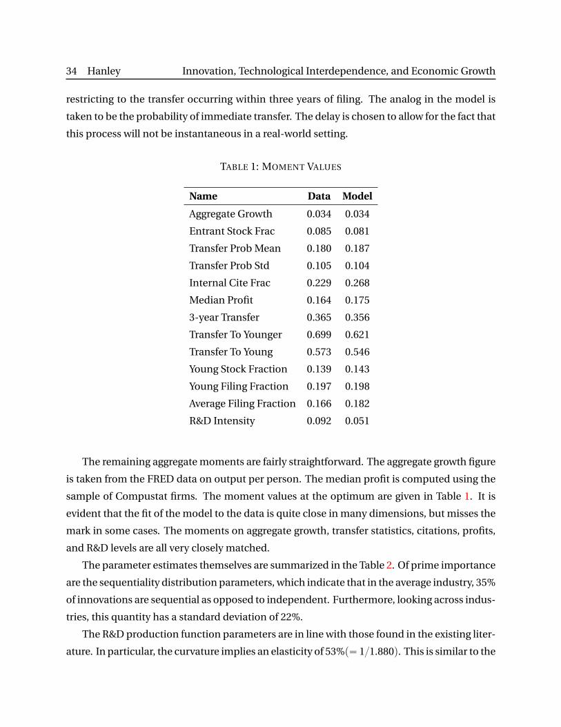
34 Hanley Innovation, Technological Interdependence, and Economic Growth
restricting to the transfer occurring within three years of filing. The analog in the model is
taken to be the probability of immediate transfer. The delay is chosen to allow for the fact that
this process will not be instantaneous in a real-world setting.
TABLE 1: MOMENT VALUES
Name Data Model
Aggregate Growth 0.034 0.034
Entrant Stock Frac 0.085 0.081
Transfer Prob Mean 0.180 0.187
Transfer Prob Std 0.105 0.104
Internal Cite Frac 0.229 0.268
Median Profit 0.164 0.175
3-year Transfer 0.365 0.356
Transfer To Younger 0.699 0.621
Transfer To Young 0.573 0.546
Young Stock Fraction 0.139 0.143
Young Filing Fraction 0.197 0.198
Average Filing Fraction 0.166 0.182
R&D Intensity 0.092 0.051
The remaining aggregate moments are fairly straightforward. The aggregate growth figure
is taken from the FRED data on output per person. The median profit is computed using the
sample of Compustat firms. The moment values at the optimum are given in Table 1. It is
evident that the fit of the model to the data is quite close in many dimensions, but misses the
mark in some cases. The moments on aggregate growth, transfer statistics, citations, profits,
and R&D levels are all very closely matched.
The parameter estimates themselves are summarized in the Table 2. Of prime importance
are the sequentiality distribution parameters, which indicate that in the average industry, 35%
of innovations are sequential as opposed to independent. Furthermore, looking across indus-
tries, this quantity has a standard deviation of 22%.
The R&D production function parameters are in line with those found in the existing liter-
ature. In particular, the curvature implies an elasticity of 53%p“ 11.880q. This is similar to the
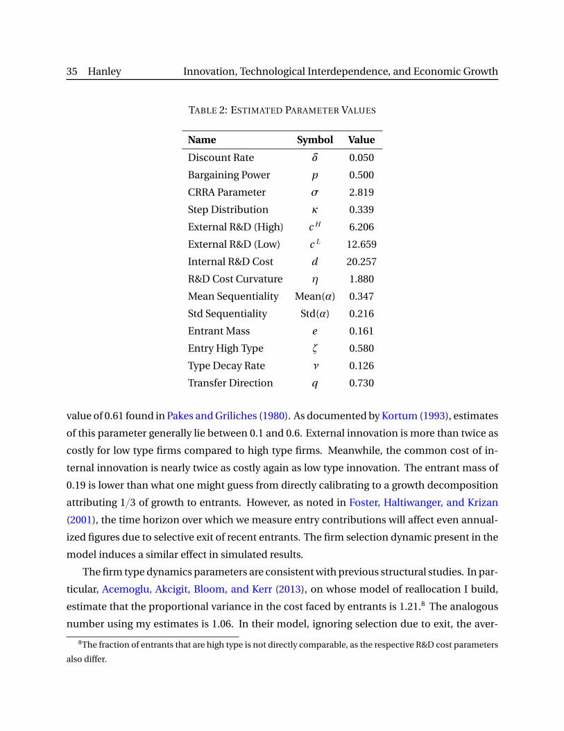
35 Hanley Innovation, Technological Interdependence, and Economic Growth
TABLE 2: ESTIMATED PARAMETER VALUES
Name Symbol Value
Discount Rate δ 0.050
Bargaining Power p 0.500
CRRA Parameter σ 2.819
Step Distribution κ 0.339
External R&D (High) c H 6.206
External R&D (Low) c L 12.659
Internal R&D Cost d 20.257
R&D Cost Curvature η 1.880
Mean Sequentiality Mean(α) 0.347
Std Sequentiality Std(α) 0.216
Entrant Mass e 0.161
Entry High Type ζ 0.580
Type Decay Rate ν 0.126
Transfer Direction q 0.730
value of 0.61 found in Pakes and Griliches (1980). As documented by Kortum (1993), estimates
of this parameter generally lie between 0.1 and 0.6. External innovation is more than twice as
costly for low type firms compared to high type firms. Meanwhile, the common cost of in-
ternal innovation is nearly twice as costly again as low type innovation. The entrant mass of
0.19 is lower than what one might guess from directly calibrating to a growth decomposition
attributing 13 of growth to entrants. However, as noted in Foster, Haltiwanger, and Krizan
(2001), the time horizon over which we measure entry contributions will affect even annual-
ized figures due to selective exit of recent entrants. The firm selection dynamic present in the
model induces a similar effect in simulated results.
The firm type dynamics parameters are consistent with previous structural studies. In par-
ticular, Acemoglu, Akcigit, Bloom, and Kerr (2013), on whose model of reallocation I build,
estimate that the proportional variance in the cost faced by entrants is 1.21.8 The analogous
number using my estimates is 1.06. In their model, ignoring selection due to exit, the aver-
8The fraction of entrants that are high type is not directly comparable, as the respective R&D cost parameters
also differ.
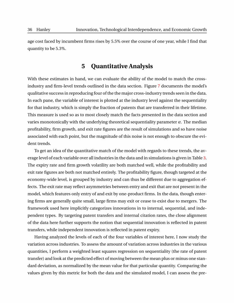
36 Hanley Innovation, Technological Interdependence, and Economic Growth
age cost faced by incumbent firms rises by 5.5% over the course of one year, while I find that
quantity to be 5.3%.
5 Quantitative Analysis
With these estimates in hand, we can evaluate the ability of the model to match the cross-
industry and firm-level trends outlined in the data section. Figure 7 documents the model’s
qualitative success in reproducing four of the the major cross-industry trends seen in the data.
In each pane, the variable of interest is plotted at the industry level against the sequentiality
for that industry, which is simply the fraction of patents that are transferred in their lifetime.
This measure is used so as to most closely match the facts presented in the data section and
varies monotonically with the underlying theoretical sequentiality parameter α. The median
profitability, firm growth, and exit rate figures are the result of simulations and so have noise
associated with each point, but the magnitude of this noise is not enough to obscure the evi-
dent trends.
To get an idea of the quantitative match of the model with regards to these trends, the av-
erage level of each variable over all industries in the data and in simulations is given in Table 3.
The expiry rate and firm growth volatility are both matched well, while the profitability and
exit rate figures are both not matched entirely. The profitability figure, though targeted at the
economy-wide level, is grouped by industry and can thus be different due to aggregation ef-
fects. The exit rate may reflect asymmetries between entry and exit that are not present in the
model, which features only entry of and exit by one-product firms. In the data, though enter-
ing firms are generally quite small, large firms may exit or cease to exist due to mergers. The
framework used here implicitly categorizes innovations in to internal, sequential, and inde-
pendent types. By targeting patent transfers and internal citation rates, the close alignment
of the data here further supports the notion that sequential innovation is reflected in patent
transfers, while independent innovation is reflected in patent expiry.
Having analyzed the levels of each of the four variables of interest here, I now study the
variation across industries. To assess the amount of variation across industries in the various
quantities, I perform a weighted least squares regression on sequentiality (the rate of patent
transfer) and look at the predicted effect of moving between the mean plus or minus one stan-
dard deviation, as normalized by the mean value for that particular quantity. Comparing the
values given by this metric for both the data and the simulated model, I can assess the pre-
37 Hanley Innovation, Technological Interdependence, and Economic Growth
FIGURE 7: CROSS-INDUSTRY PREDICTIONS
dictive power of the model. It is important to note that though the variation in sequential-
ity was targeted, variation in the other quantities has not been, meaning these implications
come purely from the model structure. Using this metric, the model can account for approxi-
mately 65% of the variation in profitability (return on sales), 26% of the variation in firm growth
volatility (employment), and 40% of the variation in exit rates. Meanwhile, the level of varia-
tion in expiry rates is overpredicted by the model. In Figure 8, I plot the proportional varia-
tion for each quantity. Both the data and model generated numbers are normalized by their
respective mean values, as is the regression line for the data.
Figure 9 depicts a number of equilibrium variables of interest as they vary with industry
sequentiality. Of particular interest in this framework is the effect of industry sequentiality on
the incentives to innovate and the resulting innovation rates. The effect on external innova-
tion is ex ante ambiguous due to the existence of two opposing forces on the expected product
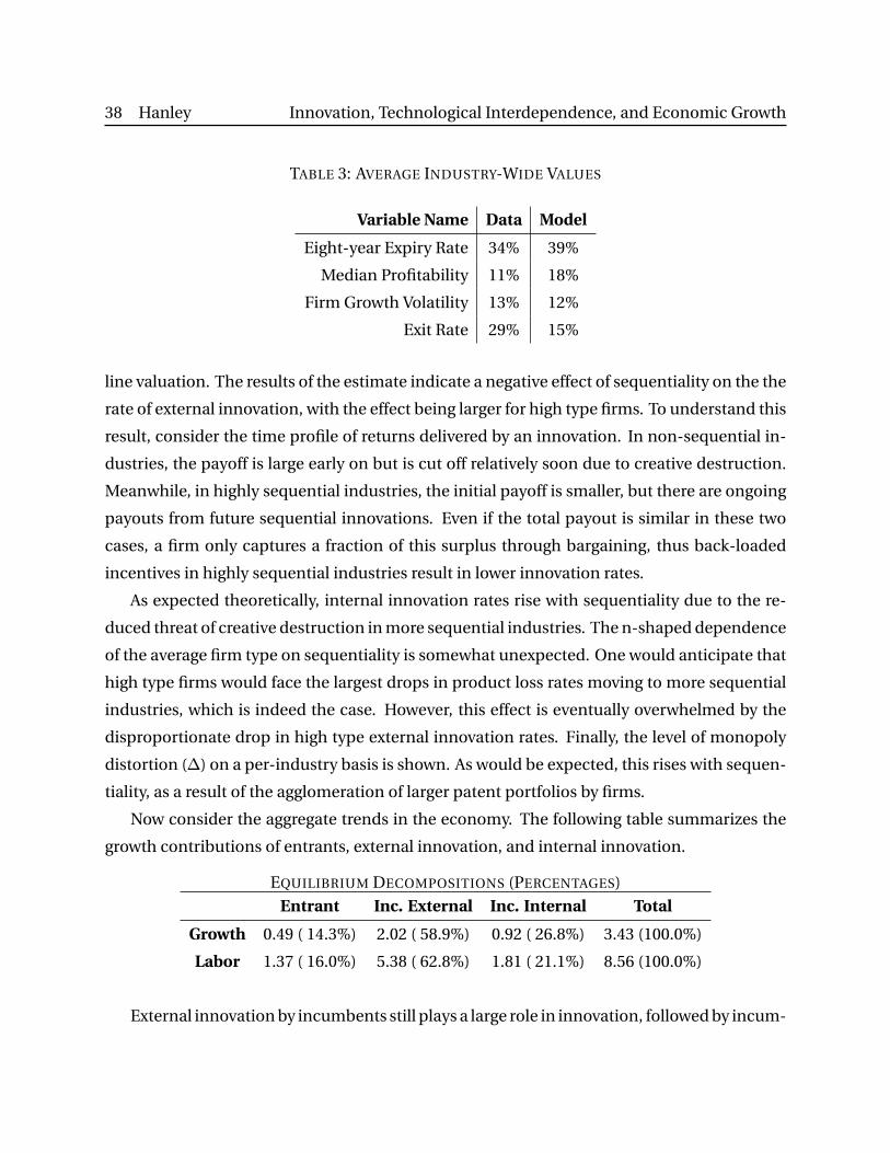
38 Hanley Innovation, Technological Interdependence, and Economic Growth
TABLE 3: AVERAGE INDUSTRY-WIDE VALUES
Variable Name Data Model
Eight-year Expiry Rate 34% 39%
Median Profitability 11% 18%
Firm Growth Volatility 13% 12%
Exit Rate 29% 15%
line valuation. The results of the estimate indicate a negative effect of sequentiality on the the
rate of external innovation, with the effect being larger for high type firms. To understand this
result, consider the time profile of returns delivered by an innovation. In non-sequential in-
dustries, the payoff is large early on but is cut off relatively soon due to creative destruction.
Meanwhile, in highly sequential industries, the initial payoff is smaller, but there are ongoing
payouts from future sequential innovations. Even if the total payout is similar in these two
cases, a firm only captures a fraction of this surplus through bargaining, thus back-loaded
incentives in highly sequential industries result in lower innovation rates.
As expected theoretically, internal innovation rates rise with sequentiality due to the re-
duced threat of creative destruction in more sequential industries. The n-shaped dependence
of the average firm type on sequentiality is somewhat unexpected. One would anticipate that
high type firms would face the largest drops in product loss rates moving to more sequential
industries, which is indeed the case. However, this effect is eventually overwhelmed by the
disproportionate drop in high type external innovation rates. Finally, the level of monopoly
distortion (∆) on a per-industry basis is shown. As would be expected, this rises with sequen-
tiality, as a result of the agglomeration of larger patent portfolios by firms.
Now consider the aggregate trends in the economy. The following table summarizes the
growth contributions of entrants, external innovation, and internal innovation.
EQUILIBRIUM DECOMPOSITIONS (PERCENTAGES)
Entrant Inc. External Inc. Internal Total
Growth 0.49 ( 14.3%) 2.02 ( 58.9%) 0.92 ( 26.8%) 3.43 (100.0%)
Labor 1.37 ( 16.0%) 5.38 ( 62.8%) 1.81 ( 21.1%) 8.56 (100.0%)
External innovation by incumbents still plays a large role in innovation, followed by incum-
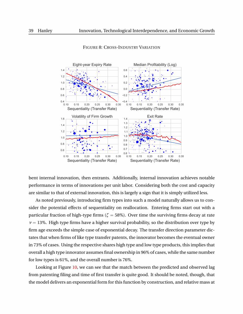
39 Hanley Innovation, Technological Interdependence, and Economic Growth
FIGURE 8: CROSS-INDUSTRY VARIATION
bent internal innovation, then entrants. Additionally, internal innovation achieves notable
performance in terms of innovations per unit labor. Considering both the cost and capacity
are similar to that of external innovation, this is largely a sign that it is simply utilized less.
As noted previously, introducing firm types into such a model naturally allows us to con-
sider the potential effects of sequentiality on reallocation. Entering firms start out with a
particular fraction of high-type firms (ζ “ 58%). Over time the surviving firms decay at rate
ν “ 13%. High type firms have a higher survival probability, so the distribution over type by
firm age exceeds the simple case of exponential decay. The transfer direction parameter dic-
tates that when firms of like type transfer patents, the innovator becomes the eventual owner
in 73% of cases. Using the respective shares high type and low type products, this implies that
overall a high type innovator assumes final ownership in 96% of cases, while the same number
for low types is 61%, and the overall number is 76%.
Looking at Figure 10, we can see that the match between the predicted and observed lag
from patenting filing and time of first transfer is quite good. It should be noted, though, that
the model delivers an exponential form for this function by construction, and relative mass at
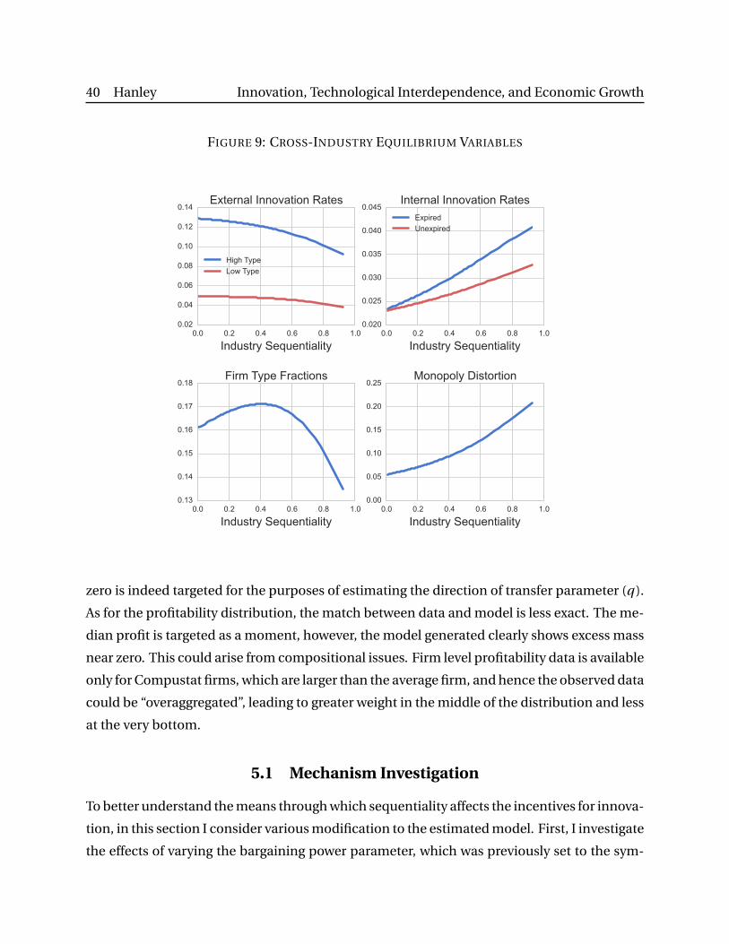
40 Hanley Innovation, Technological Interdependence, and Economic Growth
FIGURE 9: CROSS-INDUSTRY EQUILIBRIUM VARIABLES
zero is indeed targeted for the purposes of estimating the direction of transfer parameter (q ).
As for the profitability distribution, the match between data and model is less exact. The me-
dian profit is targeted as a moment, however, the model generated clearly shows excess mass
near zero. This could arise from compositional issues. Firm level profitability data is available
only for Compustat firms, which are larger than the average firm, and hence the observed data
could be “overaggregated”, leading to greater weight in the middle of the distribution and less
at the very bottom.
5.1 Mechanism Investigation
To better understand the means through which sequentiality affects the incentives for innova-
tion, in this section I consider various modification to the estimated model. First, I investigate
the effects of varying the bargaining power parameter, which was previously set to the sym-
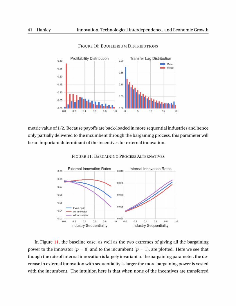
41 Hanley Innovation, Technological Interdependence, and Economic Growth
FIGURE 10: EQUILIBRIUM DISTRIBUTIONS
metric value of 12. Because payoffs are back-loaded in more sequential industries and hence
only partially delivered to the incumbent through the bargaining process, this parameter will
be an important determinant of the incentives for external innovation.
FIGURE 11: BARGAINING PROCESS ALTERNATIVES
In Figure 11, the baseline case, as well as the two extremes of giving all the bargaining
power to the innovator (p “ 0) and to the incumbent (p “ 1), are plotted. Here we see that
though the rate of internal innovation is largely invariant to the bargaining parameter, the de-
crease in external innovation with sequentiality is larger the more bargaining power is vested
with the incumbent. The intuition here is that when none of the incentives are transferred
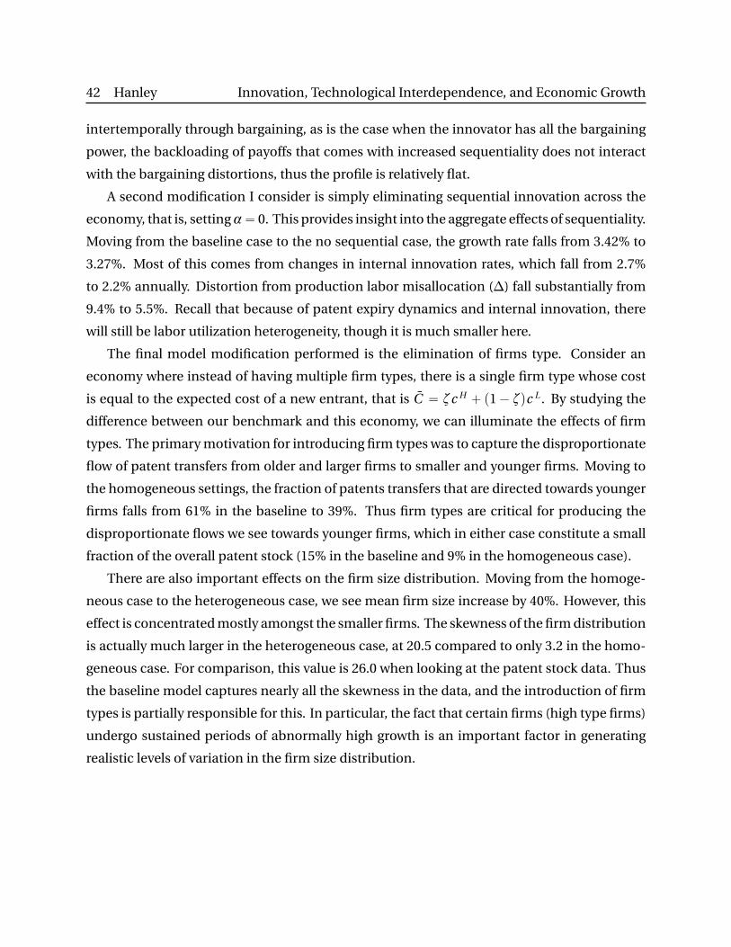
42 Hanley Innovation, Technological Interdependence, and Economic Growth
intertemporally through bargaining, as is the case when the innovator has all the bargaining
power, the backloading of payoffs that comes with increased sequentiality does not interact
with the bargaining distortions, thus the profile is relatively flat.
A second modification I consider is simply eliminating sequential innovation across the
economy, that is, settingα“ 0. This provides insight into the aggregate effects of sequentiality.
Moving from the baseline case to the no sequential case, the growth rate falls from 3.42% to
3.27%. Most of this comes from changes in internal innovation rates, which fall from 2.7%
to 2.2% annually. Distortion from production labor misallocation (∆) fall substantially from
9.4% to 5.5%. Recall that because of patent expiry dynamics and internal innovation, there
will still be labor utilization heterogeneity, though it is much smaller here.
The final model modification performed is the elimination of firms type. Consider an
economy where instead of having multiple firm types, there is a single firm type whose cost
is equal to the expected cost of a new entrant, that is C “ ζc H ` p1´ ζqc L . By studying the
difference between our benchmark and this economy, we can illuminate the effects of firm
types. The primary motivation for introducing firm types was to capture the disproportionate
flow of patent transfers from older and larger firms to smaller and younger firms. Moving to
the homogeneous settings, the fraction of patents transfers that are directed towards younger
firms falls from 61% in the baseline to 39%. Thus firm types are critical for producing the
disproportionate flows we see towards younger firms, which in either case constitute a small
fraction of the overall patent stock (15% in the baseline and 9% in the homogeneous case).
There are also important effects on the firm size distribution. Moving from the homoge-
neous case to the heterogeneous case, we see mean firm size increase by 40%. However, this
effect is concentrated mostly amongst the smaller firms. The skewness of the firm distribution
is actually much larger in the heterogeneous case, at 20.5 compared to only 3.2 in the homo-
geneous case. For comparison, this value is 26.0 when looking at the patent stock data. Thus
the baseline model captures nearly all the skewness in the data, and the introduction of firm
types is partially responsible for this. In particular, the fact that certain firms (high type firms)
undergo sustained periods of abnormally high growth is an important factor in generating
realistic levels of variation in the firm size distribution.
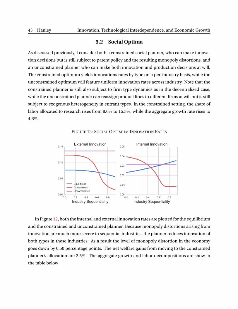
43 Hanley Innovation, Technological Interdependence, and Economic Growth
5.2 Social Optima
As discussed previously, I consider both a constrained social planner, who can make innova-
tion decisions but is still subject to patent policy and the resulting monopoly distortions, and
an unconstrained planner who can make both innovation and production decisions at will.
The constrained optimum yields innovations rates by type on a per-industry basis, while the
unconstrained optimum will feature uniform innovation rates across industry. Note that the
constrained planner is still also subject to firm type dynamics as in the decentralized case,
while the unconstrained planner can reassign product lines to different firms at will but is still
subject to exogenous heterogeneity in entrant types. In the constrained setting, the share of
labor allocated to research rises from 8.6% to 15.3%, while the aggregate growth rate rises to
4.6%.
FIGURE 12: SOCIAL OPTIMUM INNOVATION RATES
In Figure 12, both the internal and external innovation rates are plotted for the equilibrium
and the constrained and unconstrained planner. Because monopoly distortions arising from
innovation are much more severe in sequential industries, the planner reduces innovation of
both types in these industries. As a result the level of monopoly distortion in the economy
goes down by 0.50 percentage points. The net welfare gains from moving to the constrained
planner’s allocation are 2.5%. The aggregate growth and labor decompositions are show in
the table below
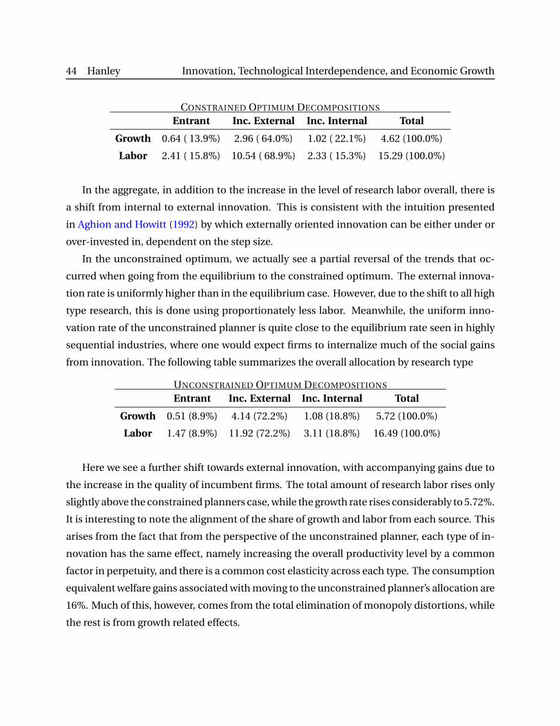
44 Hanley Innovation, Technological Interdependence, and Economic Growth
CONSTRAINED OPTIMUM DECOMPOSITIONS
Entrant Inc. External Inc. Internal Total
Growth 0.64 ( 13.9%) 2.96 ( 64.0%) 1.02 ( 22.1%) 4.62 (100.0%)
Labor 2.41 ( 15.8%) 10.54 ( 68.9%) 2.33 ( 15.3%) 15.29 (100.0%)
In the aggregate, in addition to the increase in the level of research labor overall, there is
a shift from internal to external innovation. This is consistent with the intuition presented
in Aghion and Howitt (1992) by which externally oriented innovation can be either under or
over-invested in, dependent on the step size.
In the unconstrained optimum, we actually see a partial reversal of the trends that oc-
curred when going from the equilibrium to the constrained optimum. The external innova-
tion rate is uniformly higher than in the equilibrium case. However, due to the shift to all high
type research, this is done using proportionately less labor. Meanwhile, the uniform inno-
vation rate of the unconstrained planner is quite close to the equilibrium rate seen in highly
sequential industries, where one would expect firms to internalize much of the social gains
from innovation. The following table summarizes the overall allocation by research type
UNCONSTRAINED OPTIMUM DECOMPOSITIONS
Entrant Inc. External Inc. Internal Total
Growth 0.51 (8.9%) 4.14 (72.2%) 1.08 (18.8%) 5.72 (100.0%)
Labor 1.47 (8.9%) 11.92 (72.2%) 3.11 (18.8%) 16.49 (100.0%)
Here we see a further shift towards external innovation, with accompanying gains due to
the increase in the quality of incumbent firms. The total amount of research labor rises only
slightly above the constrained planners case, while the growth rate rises considerably to 5.72%.
It is interesting to note the alignment of the share of growth and labor from each source. This
arises from the fact that from the perspective of the unconstrained planner, each type of in-
novation has the same effect, namely increasing the overall productivity level by a common
factor in perpetuity, and there is a common cost elasticity across each type. The consumption
equivalent welfare gains associated with moving to the unconstrained planner’s allocation are
16%. Much of this, however, comes from the total elimination of monopoly distortions, while
the rest is from growth related effects.
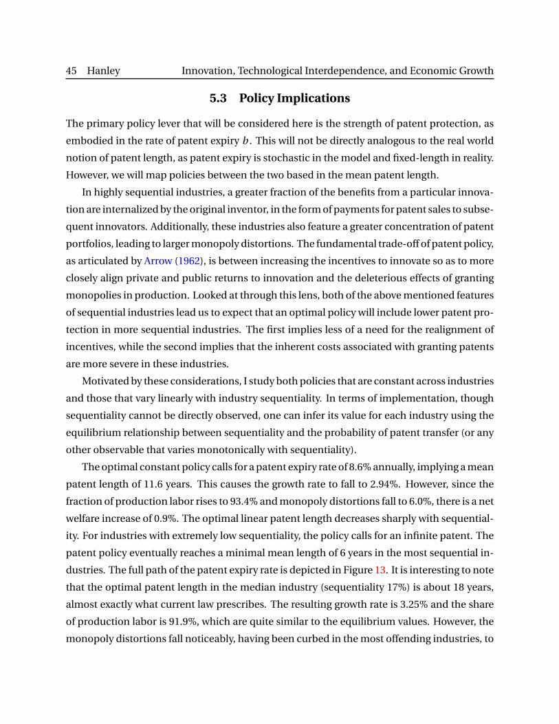
45 Hanley Innovation, Technological Interdependence, and Economic Growth
5.3 Policy Implications
The primary policy lever that will be considered here is the strength of patent protection, as
embodied in the rate of patent expiry b . This will not be directly analogous to the real world
notion of patent length, as patent expiry is stochastic in the model and fixed-length in reality.
However, we will map policies between the two based in the mean patent length.
In highly sequential industries, a greater fraction of the benefits from a particular innova-
tion are internalized by the original inventor, in the form of payments for patent sales to subse-
quent innovators. Additionally, these industries also feature a greater concentration of patent
portfolios, leading to larger monopoly distortions. The fundamental trade-off of patent policy,
as articulated by Arrow (1962), is between increasing the incentives to innovate so as to more
closely align private and public returns to innovation and the deleterious effects of granting
monopolies in production. Looked at through this lens, both of the above mentioned features
of sequential industries lead us to expect that an optimal policy will include lower patent pro-
tection in more sequential industries. The first implies less of a need for the realignment of
incentives, while the second implies that the inherent costs associated with granting patents
are more severe in these industries.
Motivated by these considerations, I study both policies that are constant across industries
and those that vary linearly with industry sequentiality. In terms of implementation, though
sequentiality cannot be directly observed, one can infer its value for each industry using the
equilibrium relationship between sequentiality and the probability of patent transfer (or any
other observable that varies monotonically with sequentiality).
The optimal constant policy calls for a patent expiry rate of 8.6% annually, implying a mean
patent length of 11.6 years. This causes the growth rate to fall to 2.94%. However, since the
fraction of production labor rises to 93.4% and monopoly distortions fall to 6.0%, there is a net
welfare increase of 0.9%. The optimal linear patent length decreases sharply with sequential-
ity. For industries with extremely low sequentiality, the policy calls for an infinite patent. The
patent policy eventually reaches a minimal mean length of 6 years in the most sequential in-
dustries. The full path of the patent expiry rate is depicted in Figure 13. It is interesting to note
that the optimal patent length in the median industry (sequentiality 17%) is about 18 years,
almost exactly what current law prescribes. The resulting growth rate is 3.25% and the share
of production labor is 91.9%, which are quite similar to the equilibrium values. However, the
monopoly distortions fall noticeably, having been curbed in the most offending industries, to
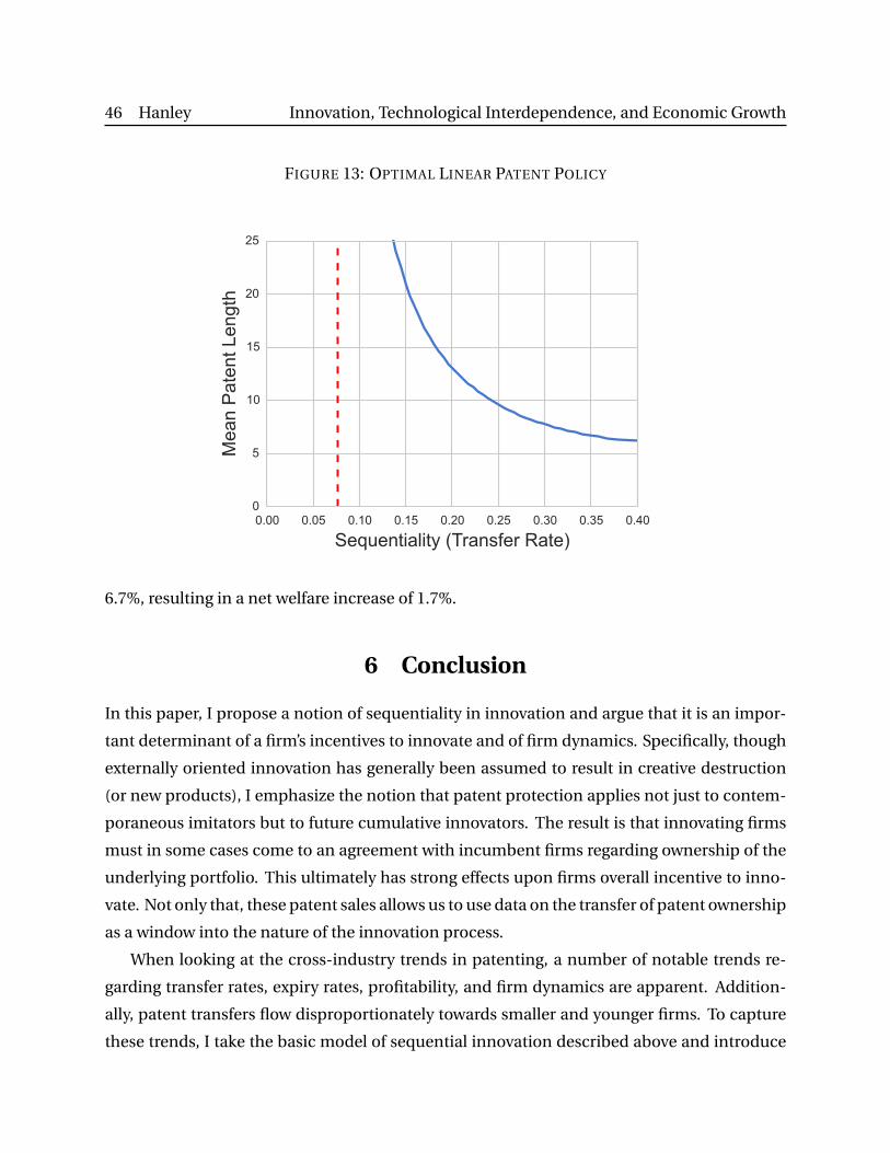
46 Hanley Innovation, Technological Interdependence, and Economic Growth
FIGURE 13: OPTIMAL LINEAR PATENT POLICY
6.7%, resulting in a net welfare increase of 1.7%.
6 Conclusion
In this paper, I propose a notion of sequentiality in innovation and argue that it is an impor-
tant determinant of a firm’s incentives to innovate and of firm dynamics. Specifically, though
externally oriented innovation has generally been assumed to result in creative destruction
(or new products), I emphasize the notion that patent protection applies not just to contem-
poraneous imitators but to future cumulative innovators. The result is that innovating firms
must in some cases come to an agreement with incumbent firms regarding ownership of the
underlying portfolio. This ultimately has strong effects upon firms overall incentive to inno-
vate. Not only that, these patent sales allows us to use data on the transfer of patent ownership
as a window into the nature of the innovation process.
When looking at the cross-industry trends in patenting, a number of notable trends re-
garding transfer rates, expiry rates, profitability, and firm dynamics are apparent. Addition-
ally, patent transfers flow disproportionately towards smaller and younger firms. To capture
these trends, I take the basic model of sequential innovation described above and introduce
47 Hanley Innovation, Technological Interdependence, and Economic Growth
heterogeneity both across industries and across firms within industry. The resulting estimated
model is able to match these trends qualitatively and account for a large fraction of the cross-
industry variation.
The quantitative estimates point to an underallocation in the quantity of labor devoted
to research. This result is not surprising given the existing theoretical and empirical litera-
ture. However, even fixing the quantity of labor devoted to research, there is a misallocation
of research labor towards those industries with the highest sequentiality. I find that monopoly
distortions are quantitatively important in this setting. In highly sequential industries, firms
accumulate large patent portfolios, allowing them acquire a substantial technological lead
over their nearest legal competitor. To remedy these misallocations in both research and pro-
duction, I introduce both constant and industry dependent patent policies and evaluate their
welfare effects.
I find that a patent policy featuring weaker patent protection in more sequential indus-
tries can generate large welfare gains over both current policy and the optimal uniform patent
policy. The implications of this finding are not out of line with certain existing proposals by
policymakers. In particular, there have been numerous calls by interest groups to either elimi-
nate or severely restrict patenting of software, an industry which I find to be highly sequential.
Other authors, such as Boldrin and Levine (2008), who advocate the elimination of patents
frequently cite the software industry as an example of patenting gone wrong. Similarly, those
concerned about “patent trolls” cite software as an industry which has been hit particularly
hard by costs associated with intellectual property litigation.9 Though I do not address these
costs directly, reducing patent protection in these industries would limit the potential damage
that patent trolls could cause.
Though this paper takes a very detailed approach to modeling patenting dynamics and the
incentives to innovate, this setting is undoubtedly extremely complex, featuring a large quan-
tity of heterogeneity both at the firm and industry level. There are many potential avenues of
research that remain to explored. For instance, the notion of sequentiality may be related to
patent breadth, meaning there are patent policy levers in addition to length that could be ex-
plored in this context. Additionally, not all innovation is necessarily protected with patenting.
Incorporating an endogenous decision to patent (as opposed to using secrecy, for instance)
could have interesting implications, though observability is naturally an issue.
9http://www.schumer.senate.gov/record.cfm?id=341612&
48 Hanley Innovation, Technological Interdependence, and Economic Growth
References
D. Acemoglu, U. Akcigit, N. Bloom, and W. R. Kerr. Innovation, Reallocation and Growth.
Working Paper 18993, NBER, April 2013.
P. Aghion and P. Howitt. A Model of Growth Through Creative Destruction. Econometrica, 60
(2):323–351, 1992.
P. Aghion, U. Akcigit, and P. Howitt. What Do We Learn From Schumpeterian Growth Theory?
Working Paper 18824, NBER, February 2013.
U. Akcigit and W. R. Kerr. Growth Through Heterogeneous Innovations. Working Paper 16443,
NBER, November 2010.
U. Akcigit, M. A. Celik, and J. Greenwood. Buy, Keep or Sell: Economic Growth and the Market
for Ideas. 2013.
K. Arrow. Economic Welfare and the Allocation of Resources for Invention. In The Rate and
Direction of Inventive Activity: Economic and Social Factors, pages 609–626. NBER, 1962.
A. Atkeson and A. T. Burstein. Innovation, Firm Dynamics, and International Trade. Journal
of Political Economy, 118(3):433–484, 2010.
J. Bessen and E. Maskin. Sequential Innovation, Patents, and Imitation. RAND Journal of
Economics, 40(4):611–635, 2009.
J. Bessen and M. J. Meurer. Patent Failure: How Judges, Bureaucrats, and Lawyers Put Innova-
tors at Risk. Princeton University Press, 2008.
N. Bloom. The Impact of Uncertainty Shocks. Econometrica, 77(3):623–685, 2009.
M. Boldrin and D. K. Levine. Against Intellectual Monopoly. Cambridge University Press, 2008.
S. J. Davis, J. Haltiwanger, and S. Schuh. Job Creation and Destruction. The MIT Press, 1998.
D. Dykeman and D. Kopko. Recording Patent License Agreements in the USPTO. Intellectual
Property Today, August, 18:19, 2004.
N. Figueroa and C. J. Serrano. Patent Trading Flows of Small and Large Firms. Working Paper
18982, NBER, April 2013.
49 Hanley Innovation, Technological Interdependence, and Economic Growth
L. Foster, J. C. Haltiwanger, and C. J. Krizan. Aggregate Productivity Growth: Lessons From
Microeconomic Evidence. In New Developments in Productivity Analysis, pages 303–372.
University of Chicago Press, 2001.
S. Graham and S. Vishnubhakat. Of Smart Phone Wars and Software Patents. Journal of Eco-
nomic Perspectives, 27(1):67–85, 2013.
J. R. Green and S. Scotchmer. On the Division of Profit in Sequential Innovation. RAND Journal
of Economics, 26(1):20–33, 1995.
Z. Griliches. Patent Statistics as Economic Indicators: A Survey. In R&D and Productivity: The
Econometric Evidence, pages 287–343. University of Chicago Press, 1998.
G. M. Grossman and E. Helpman. Quality Ladders in the Theory of Growth. Review of Eco-
nomic Studies, 58(1):43–61, 1991.
B. H. Hall, A. B. Jaffe, and M. Trajtenberg. The NBER Patent Citation Data File: Lessons, Insights
and Methodological Tools. Technical report, NBER, 2001.
H. Hopenhayn, G. Llobet, and M. Mitchell. Rewarding Sequential Innovators: Prizes, Patents,
and Buyouts. Journal of Political Economy, 114(6):1041–1068, 2006.
T. J. Klette and S. Kortum. Innovating Firms and Aggregate Innovation. Journal of Political
Economy, 112(5):986, 2004.
S. Kortum. Equilibrium R&D and the Patent–R&D Ratio: US Evidence. American Economic
Review, 83(2):450–457, 1993.
S. Kortum. Research, Patenting, and Technological Change. Econometrica, 65(6):1389–1420,
1997.
J. Laitner and D. Stolyarov. Derivative Ideas and the Value of Intangible Assets. International
Economic Review, 54(1):59–95, 2013.
R. Lentz and D. T. Mortensen. An Empirical Model of Growth Through Product Innovation.
Econometrica, 76(6):1317–1373, 2008.
A. Pakes and Z. Griliches. Patents and R&D at the Firm Level: A First Report. Economics Letters,
5(4):377–381, 1980.
50 Hanley Innovation, Technological Interdependence, and Economic Growth
A. Pakes and M. Schankerman. The Rate of Obsolescence of Patents, Research Gestation Lags,
and the Private Rate of Return to Research Resources. In R & D, Patents, and Productivity,
pages 73–88. University of Chicago Press, 1984.
A. S. Pakes. Patents as Options: Some Estimates of the Value of Holding European Patent
Stocks. Econometrica, 54(4):755–84, 1986.
G. M. Phillips and A. Zhdanov. R&D and the Incentives from Merger and Acquisition Activity.
Review of Financial Studies, 26(1):34–78, 2013.
M. J. Powell. A Hybrid Method For Nonlinear Equations. Numerical Methods for Nonlinear
Algebraic Equations, 7:87–114, 1970.
P. M. Romer. Endogenous Technological Change. Journal of Political Economy, 98(5):S71–102,
1990.
F. M. Scherer. Firm Size, Market Structure, Opportunity, and the Output of Patented Inven-
tions. American Economic Review, 55(5):1097–1125, 1965.
W. I. Zangwill and C. Garcia. Pathways to Solutions, Fixed Points, and Equilibria, 1981.
Appendices
A Data Construction
Name Matching The following procedure is used to match firm entities by name from both
the US patent data and Compustat balance sheet information
1. Remove non-corporate entities
2. Drop corporate name identifiers and common English words
3. Group and standardizing suspected acronyms
4. Construct a similarity score basic on token and positional information for each pair of
names
51 Hanley Innovation, Technological Interdependence, and Economic Growth
5. Group names by a given cutoff similarity score.
As noted by Hall, Jaffe, and Trajtenberg (2001), weighting tokens by their frequency of ap-
pearance would enhance match. The fact that certain uncommon words (such as “Samsung”)
appear in so many patents may skew this process, so an iterative is needed.
B Two Type Model
I now introduce heterogeneity amongst firms in the form of persistent types in order to ex-
plain trends regarding innovation, firm growth, and patent transfers between and amongst
large/small and young/old firms. Much of the previous derivations carry through here. The
production environment, in particular, is identical.
One major difference that arises when introducing firm-level heterogeneity is that the in-
determinacy in the direction of transfer is partially broken. When a high-type and low-type
firm have a sequential interaction (in either direction), the patents are ultimately operated
entirely by the high-type firm. However, it is still the case that when two firms of common
type interact, the direction must be chosen arbitrarily. Moving to a model with a continuum
of firm types would entirely eliminate this indeterminacy, but at the cost of tractability.
Equilibrium There are two types of firms: high-intensity and low-intensity innovators, herein
referred to as high and low type, that are differentiated by their R&D cost functions. High type
firms transition to non-adopting firms at flow rate ν. Being a low type firm is an absorbing
state. Denote a generic firm type with i P tH , Lu. There is a type-specific innovation cost
function c i p¨q for external innovation. The internal innovation technology d p¨q is the same
across types. An entrant firm starts as type H with probability ζH and type L with probability
ζL “ 1´ζH .
52 Hanley Innovation, Technological Interdependence, and Economic Growth
Successful innovation yields a present value sV i . The per-product value of a firm is then
δF V Hpλq´ 9V H
pλq “ rπpλq`ΩHx `Ω
Hz
`ατp pEV Hpβλq´V H
pλqq`p1´αqτp0´V Hpλqq
` b pV H0 ´V H
pλqq`νpV Lpλq´V H
pλqq
δF V Lpλq´ 9V L
pλq “ rπpλq`ΩLx `Ω
Lz
`ατL p pEV Lpβλq´V L
pλqq`ατH p pEV Hpβλq´V L
pλqq
`p1´αqτp0´V Lpλqq` b pV L
0 ´V Lpλqq
where
pδF `τqVH
0 ´ 9V H0 “ΩH
x `ΩH0 `νpV
L0 ´V H
0 q
pδF `τqVL
0 ´9V L0 “Ω
Lx `Ω
L0
and
Ωix “max
x i
´ rw c ipx iq` x i
sV i(
Ωiz pλq “max
z i
´ rwλ´1d pz iq` z i
pErV ipβλq´V i
pλqq(
Ωi0“max
z i0
´ rw d pz i0q` z i
0pErVipβλq´V i
0 q(
As before, posit a linearly separable form
V Hpλq “ AH
´B Hλ´1
V Lpλq “ AL
´B Lλ´1
We then find for the high type
pδF ` b `p1´αqτqAH´ 9AH
“ 1`ΩHx ` b V H
0 `ν`
AL´AH
˘
pδF ` b `p1´αqτqB H´ 9B H
“ 1´ΩHz ´ατpp1`κ´1
qB H`νpB L
´B Hq
and for the low type
pδF ` b `p1´αqτqAL´ 9AL
“ 1`ΩLx ` b V L
0 `ατH p pAH
´ALq
pδF ` b `p1´αqτqB L´ 9B L
“ 1´ΩLz ´ατ
L pp1`κ´1qB L
´ατH p pB L´B H
λq
53 Hanley Innovation, Technological Interdependence, and Economic Growth
The option values of innovation be simplified to
Ωix “max
x i
´ rw c ipx iq` x i
sV i(
Ωiz “max
z i
´ rw d pz iq` z i B i
p1`κ´1q(
Ωi0“max
z i
´ rw d pz iq` z i
pAi´B i
p1`κq´V i0 q(
Now it can be verified that B H “ B L ” B . As such we will also have ΩHz “ ΩL
z ” Ωz and
z H “ z H ” z . As high type firms have a superior innovation technology, they will assume
production in the case of sequential innovation. Between firms of a common type, it is am-
biguous. The expected gain from innovation is given by
sV H“ rp1´αq`αµ0sEV H
pβq
`αp1´p q
„ż 8
1pEV H
pβλq´V HpλqqdµH
`pλq`
ż 8
1pEV H
pβλq´V LpλqqdµL
`pλq
sV L“ rp1´αq`αµ0sEV L
pβq
`αp1´p q
„ż 8
1pEV H
pβλq´V LpλqqdµH
`pλq`
ż 8
1pEV L
pβλq´V LpλqqdµL
`pλq
These can then be simplified to
sV H“ rp1´αq`αµ0spA
H´B H
p1`κqq`αp1´p q“
pµ`Γ`B Hp1`κ´1
q`µL`pAH
´ALq‰
sV L“ rp1´αq`αµ0spA
L´B H
p1`κqq`αp1´p q“
pµ`Γ`B Hp1`κ´1
q`µH`pAH
´ALq‰
Let there be a mass L of researchers. The labor market clearing condition is
1“Γ
rw`pµH
` eζHqc px H
q`pµL` eζL
qc px Lq`µH
0 d pz H0 q`µ
L0 d pz L
0 q`µ`Γ`d pz q
Steady State Imposing stationarity of values and state space elements, the firm value func-
tions simplify to
B “1
δF ` b `p1´αqτ`pατp ` z`
δ`τ`bδ`τ
˘
p1´1ηqqp1`κ´1q
and
AH“
1`ΩHx ` b V H
0 `νAL
δF ` b `p1´αqτ`νAL“
1`ΩLx ` b V L
0 `ατH p AH
δF ` b `p1´αqτ`ατH p
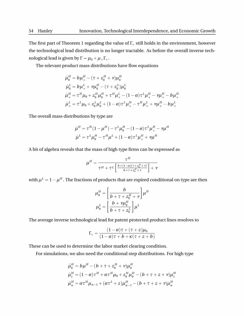
54 Hanley Innovation, Technological Interdependence, and Economic Growth
The first part of Theorem 1 regarding the value of Γ` still holds in the environment, however
the technological lead distribution is no longer tractable. As before the overall inverse tech-
nological lead is given by Γ “µ0`µ`Γ`.
The relevant product mass distributions have flow equations
9µH0 “ bµH
`´pτ` z H
0 `νqµH0
9µL0 “ bµL
``νµH
0 ´pτ` z L0 qµ
L0
9µH`“τHµ0` z H
0 µH0 `τ
HµL`´p1´αqτLµH
`´νµH
`´ bµH
`
9µL`“τLµ0` z L
0 µL0 `p1´αqτ
LµH`´τHµL
``νµH
`´ bµL
`
The overall mass distributions by type are
9µH“τH
p1´µHq´τLµH
0 ´p1´αqτLµH`´νµH
9µL“τLµH
0 ´τHµL
`p1´αqτLµH``νµH
A bit of algebra reveals that the mass of high type firms can be expressed as
µH“
τH
τH `τL
”
b`p1´αqpτ`z H0 `νq
b`τ`z H0 `ν
ı
`ν
with µL “ 1´µH . The fractions of products that are expired conditional on type are then
µH0 “
„
b
b `τ` z H0 `ν
µH
µL0 “
„
b `νµH0
b `τ` z L0
µL
The average inverse technological lead for patent protected product lines resolves to
Γ`“p1´αqτ`pτ` z qµ0
p1´αqτ` b `κpτ` z ` b q
These can be used to determine the labor market clearing condition.
For simulations, we also need the conditional step distributions. For high type
9µH0 “ bµH
´pb `τ` z H0 `νqµ
H0
9µH1 “ p1´αqτ
H`ατHµ0` z H
0 µH0 ´pb `τ` z `νqµH
1
9µHn “ατ
Hµn´1`pατL` z qµH
n´1´pb `τ` z `νqµHn
55 Hanley Innovation, Technological Interdependence, and Economic Growth
and for low type
9µL0 “ νµ
H0 ` bµL
´pb `τ` z L0 qµ
L0
9µL1 “ νµ
H1 `p1´αqτ
L`τLµ0` z L
0 µL0 ´pb `τ` z qµL
1
9µLn “ νµ
Hn `pατ
L` z qµL
n´1´pb `τ` z qµLn
These can be solved for iteratively with foreknowledge of µH and µL .
C Algorithm
Equilibrium The basic models without industry heterogeneity can be solved in a straight-
forward fashion by setting up systems of equations consisting of first order conditions and the
labor market clearing condition. These will depend on the aggregate innovation rates, so as
to allow for the direct computation of product distributions, and the wage rate.
Moving to a setting with industry heterogeneity, the algorithm can be split into two levels.
First, a wage rate is proposed, then each industry equilibrium is solved individually as in the
basic model. Finally, these solution vectors are aggregated to evaluate the overall labor mar-
ket clearing condition and the aggregate growth rate. Solving this system for the wage rate
and growth rate constitutes solving the equilibrium in its entirety. I use the Powell’s hybrid
method10 described in Powell (1970) to solve equations at both the industry level and over-
all equilibrium level. For more information on solving nonlinear systems, see Zangwill and
Garcia (1981).
Simulations Simulating firms in an efficient manner involves a small amount of further
derivation. In particular, when a firm undertakes a successful innovation, with probability
α it must purchase rights to existing technology from the incumbent, assuming said incum-
bent’s product has patent protection. In this case, if the innovating firm assumes production
(i.e., with probability q is the untyped case), the step size of the product they receive can be
drawn from the steady state distribution. In addition there will be one further innovation on
top of that.
Interestingly, since the realization of the step size value for a given patent does not affect
future patenting dynamics, these two factors will be independent in steady state as well. As-
suming step increments are Pareto distributed, the distribution of the technological lead for
10The exact code used is from the MINPACK library through the Python wrapper in SciPy.
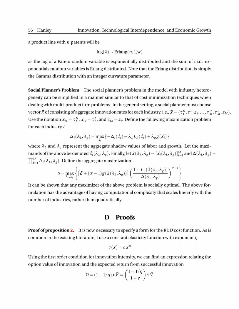
56 Hanley Innovation, Technological Interdependence, and Economic Growth
a product line with n patents will be
logpλq „ Erlangpn , 1κq
as the log of a Pareto random variable is exponentially distributed and the sum of i.i.d. ex-
ponentials random variables is Erlang distributed. Note that the Erlang distribution is simply
the Gamma distribution with an integer curvature parameter.
Social Planner’s Problem The social planner’s problem in the model with industry hetero-
geneity can be simplified in a manner similar to that of cost minimization techniques when
dealing with multi-product firm problems. In the general setting, a social planner must choose
vector ~x of consisting of aggregate innovation rates for each industry, i.e., ~x “ pτH1 ,τL
1 , z1, . . . ,τHM ,τL
M , zM q.
Use the notation xi 1“τHi , xi 2“τ
Li , and xi 3“ zi . Define the following maximization problem
for each industry i
∆i pλL ,λg q “max~xi
´∆i p~xi q´λL LR p~xi q`λg g p~xi q(
where λL and λg represent the aggregate shadow values of labor and growth. Let the maxi-
mands of the above be denoted ~xi pλL ,λg q. Finally, let ~x pλL ,λg q “ r~xi pλL ,λg qsMi“1 and∆pλL ,λg q “
śMi“1∆i pλL ,λg q. Define the aggregate maximization
S “maxλL ,λg
#
“
δ`pσ´1qg p~x pλL ,λg qq‰
ˆ
1´ LR p~x pλL ,λg qq
∆pλL ,λg q
˙σ´1+
It can be shown that any maximizer of the above problem is socially optimal. The above for-
mulation has the advantage of having computational complexity that scales linearly with the
number of industries, rather than quadratically.
D Proofs
Proof of proposition 2. It is now necessary to specify a form for the R&D cost function. As is
common in the existing literature, I use a constant elasticity function with exponent η
c px q “ c x η
Using the first order condition for innovation intensity, we can find an expression relating the
option value of innovation and the expected return from successful innovation
Ω“ p1´1ηqx sV “
ˆ
1´1η
1` e
˙
τ sV
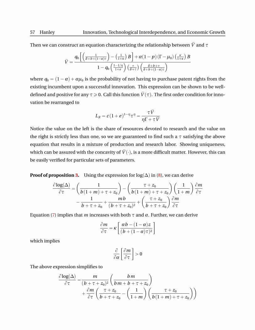
57 Hanley Innovation, Technological Interdependence, and Economic Growth
Then we can construct an equation characterizing the relationship between sV and τ
sV “
q0
”´
1δ`b`p1´αqτ
¯
´`
11`κ
˘
Bı
`αp1´p qpΓ ´µ0q`
κ1`κ
˘
B
1´q0
´
1´1η1`e
¯
`
τδ`τ
˘
´
δ`b`τδ`b`p1´αqτ
¯
where q0 “ p1´αq`αµ0 is the probability of not having to purchase patent rights from the
existing incumbent upon a successful innovation. This expression can be shown to be well-
defined and positive for any τě 0. Call this function sV pτq. The first order condition for inno-
vation be rearranged to
LR “ c p1` e q1´ητη“τ sV
ηΓ `τ sV
Notice the value on the left is the share of resources devoted to research and the value on
the right is strictly less than one, so we are guaranteed to find such a τ satisfying the above
equation that results in a mixture of production and research labor. Showing uniqueness,
which can be assured with the concavity of sV p¨q, is a more difficult matter. However, this can
be easily verified for particular sets of parameters.
Proof of proposition 3. Using the expression for logp∆q in (8), we can derive
B logp∆q
Bτ“
ˆ
1
b p1`mq`τ` z0
˙
´
ˆ
τ` z0
b p1`mq`τ` z0
˙ˆ
1
1`m
˙
Bm
Bτ
´1
b `τ` z0`
m b
pb `τ` z0q2`
ˆ
τ` z0
b `τ` z0
˙
Bm
Bτ
Equation (7) implies that m increases with both τ and α. Further, we can derive
Bm
Bτ“ κ
„
αb ´p1´αqz
pb `p1´αqτq2
which implies
B
Bα
„
Bm
Bτ
ą 0
The above expression simplifies to
B logp∆q
Bτ“
m
pb `τ` z0q2
ˆ
b m
b m ` b `τ` z0
˙
`Bm
Bτ
ˆ
τ` z0
b `τ` z0´
ˆ
1
1`m
˙ˆ
τ` z0
b p1`mq`τ` z0
˙˙
58 Hanley Innovation, Technological Interdependence, and Economic Growth
which can be seen to be increasing in α. As τ and z0 enter into the above expression in the
exact same manner, the same logic applies for z0 as well. However, z0 does not affect m , the
resulting expression is simply
B logp∆q
Bz0“
m
pb `τ` z0q2
ˆ
b m
b m ` b `τ` z0
˙
Conversely, z affects m positively but does not change the composition between expired and
unexpired product lines, meaning we find
B logp∆q
Bz“Bm
Bz
ˆ
τ` z0
b `τ` z0´
ˆ
1
1`m
˙ˆ
τ` z0
b p1`mq`τ` z0
˙˙
Varying z and z0 simultaneously would yield an expression equivalent to that for τ, where
both terms are present.