Influences on Hyporheic Exchange in a Small

Coastal British Columbia Suburban Stream

by

Jacquelyn Shrimer

B.Sc. (Environmental Science), Simon Fraser University, 2008

Thesis Submitted In Partial Fulfillment of the

Requirements for the Degree of

Master of Science

in the

Department of Geography

Faculty of Environment

Jacquelyn Shrimer 2013

SIMON FRASER UNIVERSITY

Spring 2013

ii

Approval

Name: Jacquelyn Shrimer

Degree: Master of Science (Geography)

Title of Thesis: Influences on Hyporheic Exchange in a Small Coastal British Columbia Suburban Stream

Examining Committee: Chair: Kirsten Zickfeld Assistant Professor

Dr. Ilja van Meerveld Senior Supervisor Assistant Professor Faculty of Earth and Life Sciences, VU VU University Amsterdam

Dr. Jeremy Venditti Committee Member Associate Professor, Geography Simon Fraser University

Dr. Diana Allen External Examiner Professor Department of Earth Sciences Simon Fraser University

Date Defended: March 28, 2013

iii

Partial Copyright Licence

iv

Abstract

This study examined how discharge, streambed topography, and channel

planform influence hyporheic exchange in a coastal suburban stream in B.C. Tracer

experiments were carried out in four reaches of Hoy Creek in Coquitlam using sodium

chloride, and piezometers were installed to determine the vertical hydraulic gradient

(VHG). The tracer data were used in OTIS, a transient storage model, to determine the

following parameters: cross-sectional area of the stream and storage zone, dispersion,

and the storage zone exchange coefficient (α). For the lower reaches, there was no

significant relation between α and discharge; however, there was a significant positive

relation between α and discharge for the upper reaches. Dispersion and the cross-

sectional area of the storage zone did not change with discharge. VHG and streambed

tracer breakthrough curves/data showed predominantly upwelling conditions. Hyporheic

flow occurred mainly through meander bends, step-pool systems, and riffles.

Keywords: Hyporheic exchange; suburban stream; Hoy Creek; OTIS; tracer study; vertical hydraulic gradient

v

Dedication

Soli Deo gloria.

vi

Acknowledgements

Thank you to everyone who has supported and encouraged me along the journey of

completing this degree. I would like to thank Dr. Ilja van Meerveld for providing so much

input and keeping me on track. I appreciate your direction, encouragement, and

patience, especially when it came to OTIS. I would also like to thank Dr. Jeremy Venditti

and Dr. Diana Allen for providing constructive feedback on my thesis.

Thank you to everyone who provided assistance in the field, rain or shine (Elizabeth

Baird, Naomi Cummings, Katie Dodman, Terence Lai, Tabitha Li, Jenn Melatini, Fred

Shrimer, Sheena Spencer, Louise Steinway, Tanya Witzke, and Stephan Zimmerman).

This project would not be complete without your help.

I would like to thank my parents for their support throughout this endeavor, starting with

your help in the application process from half a world away, with minimal internet and

phone access. This would not have been possible without your help.

Thanks to my family and friends for motivation, encouragement, lending a listening ear,

and putting up with my busy and ever-changing schedule. Thanks to everyone in the

Hydrology Lab and Department of Geography for the time spent bouncing ideas off one

another, whether relevant to our research or otherwise.

I would like to acknowledge NSERC for funding for this research, Metro Vancouver for

precipitation data, and the City of Coquitlam for various documents.

vii

Table of Contents

Approval .............................................................................................................................ii Partial Copyright Licence .................................................................................................. iii Abstract .............................................................................................................................iv Dedication ......................................................................................................................... v Acknowledgements ...........................................................................................................vi Table of Contents ............................................................................................................. vii List of Tables .....................................................................................................................ix List of Figures.................................................................................................................. xiii

1. Introduction ............................................................................................................ 1 1.1. Problem Statement .................................................................................................. 1 1.2. Research Objectives ................................................................................................ 3

1.2.1. Research Questions ..................................................................................... 3 1.2.2. Hypotheses ................................................................................................... 4

2. Literature Review ................................................................................................... 5 2.1. Introduction .............................................................................................................. 5 2.2. Significance of the Hyporheic Zone ......................................................................... 5 2.3. Controls on Hyporheic Exchange ............................................................................. 7

2.3.1. Discharge ..................................................................................................... 7 2.3.2. Geomorphic Features ................................................................................. 10 2.3.3. Lateral Inflow and Hillslope Topography .................................................... 12

2.4. Transport Processes and Modeling Hyporheic Exchange ..................................... 13

3. Study Site and Methodology ............................................................................... 17 3.1. Study Site ............................................................................................................... 17

3.1.1. Hoy Creek, Coquitlam ................................................................................ 17 3.1.2. Climate and Streamflow Normals ............................................................... 22 3.1.3. Description of the Study Reaches .............................................................. 23 3.1.3.1. Upper Study Reaches .......................................................................... 23 3.1.3.2. Lower Study Reaches .......................................................................... 24

3.2. Methodology ........................................................................................................... 25 3.2.1. Tracer Experiments .................................................................................... 25 3.2.2. Determination of Vertical Hydraulic Gradients ............................................ 32 3.2.3. Determination of Inflow ............................................................................... 36 3.2.4. Topographic Surveys .................................................................................. 37 3.2.5. Modeling with OTIS and OTIS-P ................................................................ 37 3.2.5.1. Calibration ............................................................................................ 37 3.2.5.2. Validation .............................................................................................. 39

4. Results and Discussion ....................................................................................... 41 4.1. Streamflow ............................................................................................................. 41 4.2. Steady State EC and Lateral Inflow ....................................................................... 42 4.3. Vertical Hydraulic Gradients ................................................................................... 51 4.4. Tracer Experiments ................................................................................................ 61

viii

4.4.1. Breakthrough Curves .................................................................................. 61 4.4.2. OTIS-P Calibration ..................................................................................... 66 4.4.3. Optimized Parameter Values ...................................................................... 69 4.4.4. Storage Zone Exchange Coefficient ........................................................... 73 4.4.5. Cross-sectional Area of the Storage Zone and Stream .............................. 75 4.4.6. Dispersion ................................................................................................... 79 4.4.7. Storage Zone Residence Time ................................................................... 80 4.4.8. Hydraulic Retention Factor and Average Traveling Distance of a

Water Molecule .......................................................................................... 81 4.5. Reliability of the Optimized Parameters ................................................................. 82 4.6. Model Validation ..................................................................................................... 84 4.7. Issues with OTIS .................................................................................................... 89

5. Conclusion and Recommendations ................................................................... 91 5.1. Conclusion ............................................................................................................. 91 5.2. Recommendations ................................................................................................. 92

References ..................................................................................................................... 95

Appendices .................................................................................................................. 101 Appendix A: Temporal Stability Calculation .................................................................. 102 Appendix B: Steady State EC Maps ............................................................................. 103 Appendix C: Calibration Results ................................................................................... 107 Appendix D: Validation Results ..................................................................................... 138

ix

List of Tables

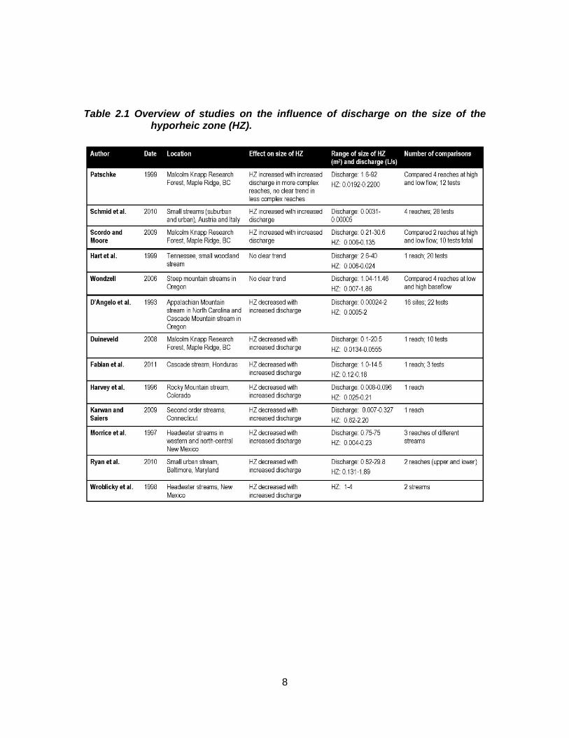
Table 2.1 Overview of studies on the influence of discharge on the size of the hyporheic zone (HZ). ....................................................................................... 8

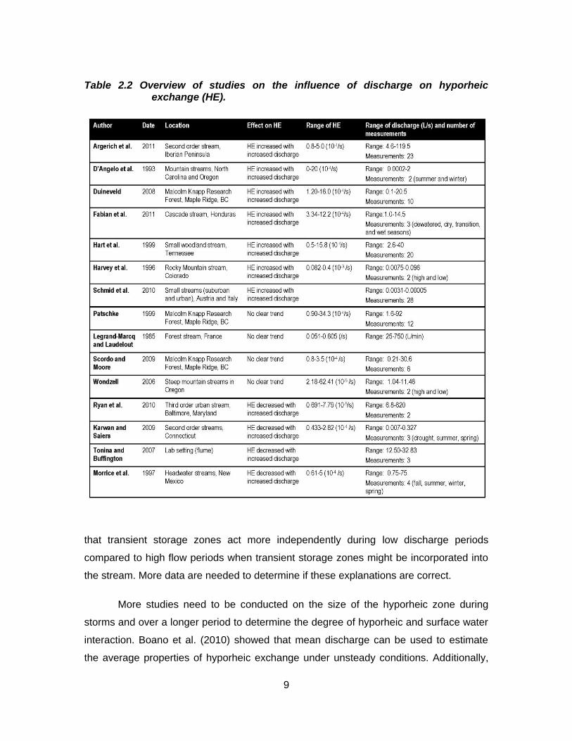
Table 2.2 Overview of studies on the influence of discharge on hyporheic exchange (HE). ............................................................................................... 9

Table 3.1 Upper (UA and UB) and lower (DA and DB) reach characteristics. ................ 18

Table 3.2 Summary of the tracer experiments in the upper reach UA (EC measurements from the YSI and *ECH2O probes; the injection stopped at an unknown time on July 7, thus the duration of injection is an estimate). ................................................................................................. 27

Table 3.3 Summary of the tracer experiments in the upper reach UB (EC measurements from the YSI and *ECH2O probes). ...................................... 27

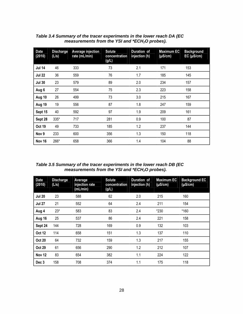
Table 3.4 Summary of the tracer experiments in the lower reach DA (EC measurements from the YSI and *ECH2O probes). ...................................... 28

Table 3.5 Summary of the tracer experiments in the lower reach DB (EC measurements from the YSI and *ECH2O probes). ...................................... 28

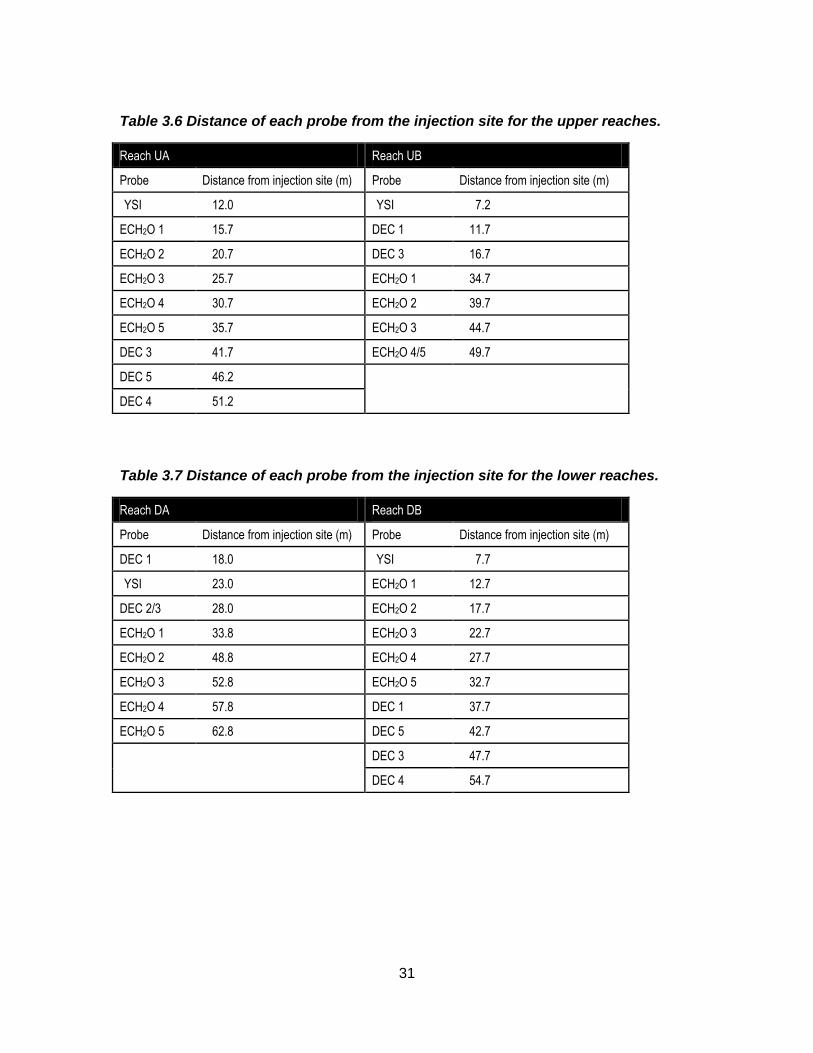
Table 3.6 Distance of each probe from the injection site for the upper reaches. ............ 31

Table 3.7 Distance of each probe from the injection site for the lower reaches. ............. 31

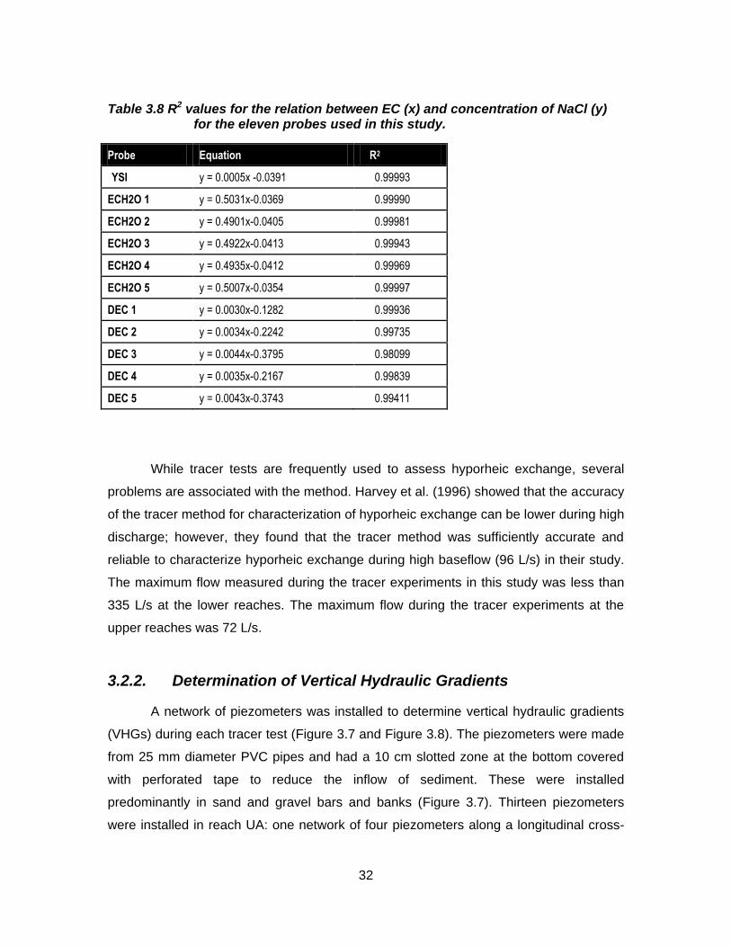
Table 3.8 R2 values for the relation between EC (x) and concentration of NaCl (y) for the eleven probes used in this study. ....................................................... 32

Table 3.9 Location and depth below the surface of the piezometers in the upper reaches UA and UB. Reach UA: piezometer 1 was installed outside of the reach. Reach UB: piezometers 2, 3, and 5 were washed away. ............. 34

Table 3.10 Location and depth below the surface of the piezometers in the lower reaches DA and DB. ..................................................................................... 35

Table 4.1 Discharge (Q), measurement uncertainty, and lateral inflow (Qlat) for the lower reach tracer tests. QYSI and YSI error are the discharge and the uncertainty in the discharge calculated from the EC measurements using the YSI probe. QE5 and E5 error are the discharge and the uncertainty in the discharge calculated from the EC measurements using the ECH2O 5 probe. In all but 5 cases (*) Qlat was less than the uncertainty in Qlat. For September 24, 2010 ECH2O data were unavailable. See Figure 3.7 and Table 3.7 for the location of the YSI and ECH2O probes. ...................................................................... 44

x

Table 4.2 Discharge (Q), measurement uncertainty, and lateral inflow (Qlat) for the upper reach tracer tests. QYSI and YSI error are the discharge and the uncertainty in the discharge calculated from the EC measurements using the YSI probe. QE5 and E5 error are the discharge and the uncertainty in the discharge calculated from the EC measurements using the ECH2O 5 probe. (*indicates calculation from ECH2O 1 probe instead of the YSI probe). In all cases Qlat was less than the uncertainty in Qlat. See Figure 3.7 and Table 3.6. ........................... 45

Table 4.3 Time between the start of the injection (start) and steady state (SS), the start of the injection and the start of the increase in EC (start to rise), between the start of the increase in the rise in EC and steady state EC (rise to SS), and the ratio of rise to SS and start to rise (normalized) for the YSI probe measurements at upper reach UA. The Spearman rank correlation coefficient (rs) for the relation between these timing parameters and discharge is also given. .................................. 62

Table 4.4 Time between the start of the injection (start) and steady state (SS), the start of the injection and the start of the increase in EC (start to rise), between the start of the increase in the rise in EC and steady state EC (rise to SS), and the ratio of rise to SS and start to rise (normalized) for the YSI probe measurements at upper reach UB. The Spearman rank correlation coefficient (rs) for the relation between these timing parameters and discharge is also given. .................................. 63

Table 4.5 Time between the start of the injection (start) and steady state (SS), the start of the injection and the start of the increase in EC (start to rise), between the start of the increase in the rise in EC and steady state (rise to SS), and the ratio of rise to SS and start to rise (normalized) for the YSI probe measurements at lower reach DA. The Spearman rank correlation coefficient (rs) for the relation between these timing parameters and discharge is also given. .................................. 64

Table 4.6 Time between the start of the injection (start) and steady state (SS), the start of the injection and the start of the increase in EC (start to rise), between the start of the increase in the rise in EC and steady state (rise to SS), and the ratio of rise to SS and start to rise (normalized) for the YSI probe measurements at lower reach DB. The Spearman rank correlation coefficient (rs) for the relation between these timing parameters and discharge is also given. .................................. 65

Table 4.7 The correlation coefficient (R), Nash-Sutcliffe Efficiency (E), and Mean Squared Error (MSE) for the modeled and observed data at the YSI probe location and the range of R, E, and MSE for the ECH2O probe locations in reach UA. For Oct. 5, 2010 only the ECH2O-1 probe recorded data. The experiment on July 7, 2010 was not included due to the pump stopping at an unknown time. ................................................... 67

xi

Table 4.8 The correlation coefficient (R), Nash-Sutcliffe Efficiency (E), and Mean Squared Error (MSE) for the modeled and observed data at the YSI probe location and the range of R, E, and MSE for the ECH2O probe locations in reach UB (Oct. 27 parameters are not included because they would not stabilize in OTIS-P; *outlier). ................................................. 68

Table 4.9 The correlation coefficient (R), Nash-Sutcliffe Efficiency (E), and Mean Squared Error (MSE) for the modeled and observed data at the YSI probe location and the range of R, E, and MSE for the ECH2O probe locations in reach DA (Sept 28 and Nov 9 parameters were not included because the model simulations would not stabilize in OTIS-P; *outlier). .................................................................................................... 68

Table 4.10 The correlation coefficient (R), Nash-Sutcliffe Efficiency (E), and Mean Squared Error (MSE) for the modeled and observed data at the YSI probe location and the range of R, E, and MSE for the ECH2O probe locations in reach DB. ......................................................................... 69

Table 4.11 The optimized parameter values for reach UA. For each date the first row shows the values for the first site (YSI probe) and second row for the last site (ECH2O 5 probe). The experiment on July 7, 2010 was not included due to the pump stopping at an unknown time. See Figure 3.7 and Table 3.6 for the probe locations. ......................................... 70

Table 4.12 The optimized parameter values for reach UB (Oct. 27 parameters are not included because they would not stabilize in OTIS-P; *outlier). For each date the first row shows the values for the first site (YSI probe) and second row for the last site (ECH2O 4/5 probe). See Figure 3.7 and Table 3.6 for the probe locations. ......................................... 71

Table 4.13 The optimized parameter values for reach DA (*estimate from a different probe location due to YSI probe malfunction; Sept. 28 and Nov. 9 parameters were not included because the model simulations would not stabilize in OTIS-P; **outlier). For each date the first row shows the values for the first site (YSI probe) and second row for the 6th site (ECH2O 5 probe). DaI for Nov. 16 is not given due to high uncertainty in the discharge calculation. See Figure 3.7 and Table 3.7 for the probe locations. .................................................................................. 72

Table 4.14 The optimized parameter values for reach DB. For each date the first row shows the values for the first site (YSI probe) and second row for the 6th site (ECH2O 5 probe). See Figure 3.7 and Table 3.7 for the probe locations. ............................................................................................. 73

Table 4.15 Correlation coefficient (R), Nash-Sutcliffe Efficiency (E), and Mean Squared Error (MSE) of the range of modeled versus observed DEC and piezometer data for reaches UA and UB (*outlier). ................................ 85

xii

Table 4.16 Correlation coefficient (R), Nash-Sutcliffe Efficiency (E), and Mean Squared Error (MSE) for the modeled and observed DEC and piezometer data for reaches DA and DB (*outlier). ....................................... 86

xiii

List of Figures

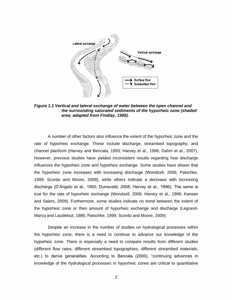
Figure 1.1 Vertical and lateral exchange of water between the open channel and the surrounding saturated sediments of the hyporheic zone (shaded area; adapted from Findlay, 1995). ................................................................. 2

Figure 2.1 The four processes of solute transport in a stream. ....................................... 13

Figure 2.2 Conceptual framework for OTIS (from Runkel, 1998). ................................... 14

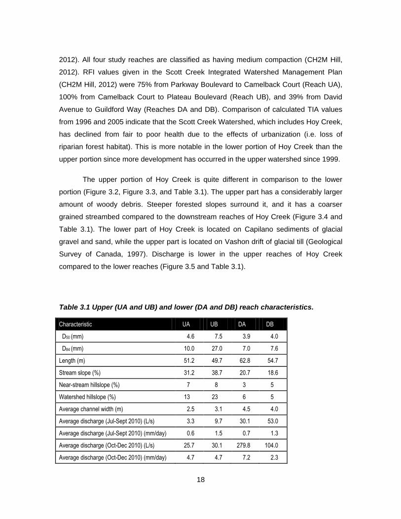
Figure 3.1 Location of Hoy Creek in Coquitlam, BC. (Data source: Google Earth, Digital Globe, accessed June 8, 2012) ......................................................... 19

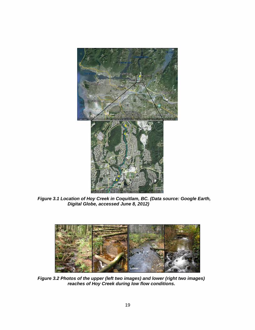
Figure 3.2 Photos of the upper (left two images) and lower (right two images) reaches of Hoy Creek during low flow conditions. ........................................ 19

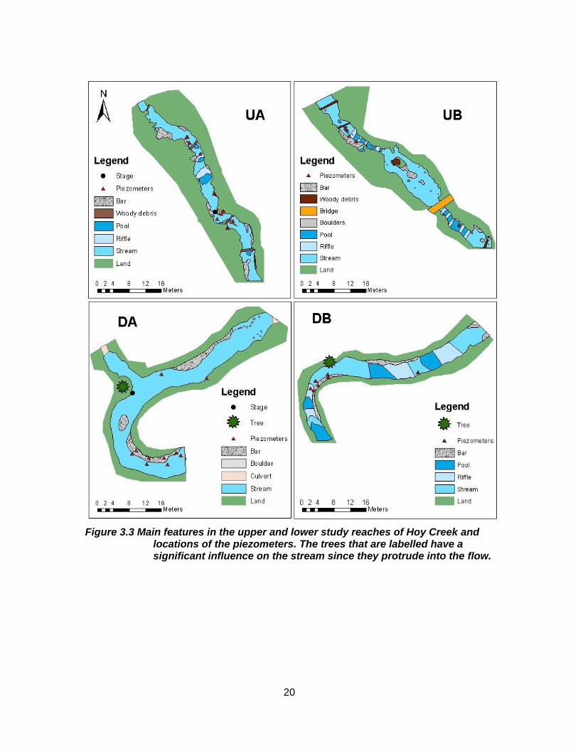
Figure 3.3 Main features in the upper and lower study reaches of Hoy Creek and locations of the piezometers. The trees that are labelled have a significant influence on the stream since they protrude into the flow. ........... 20

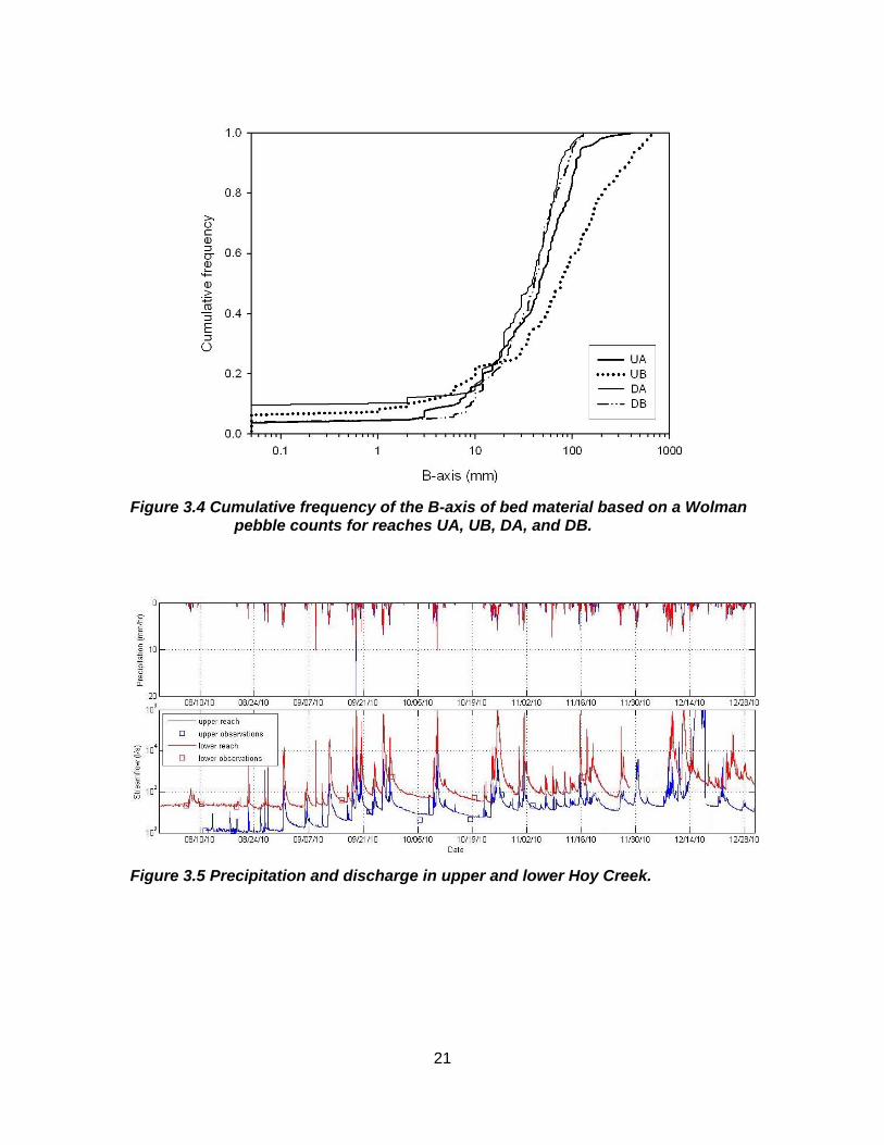
Figure 3.4 Cumulative frequency of the B-axis of bed material based on a Wolman pebble counts for reaches UA, UB, DA, and DB. ............................ 21

Figure 3.5 Precipitation and discharge in upper and lower Hoy Creek. .......................... 21

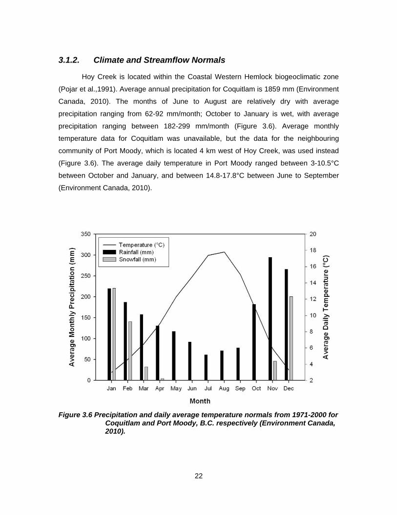
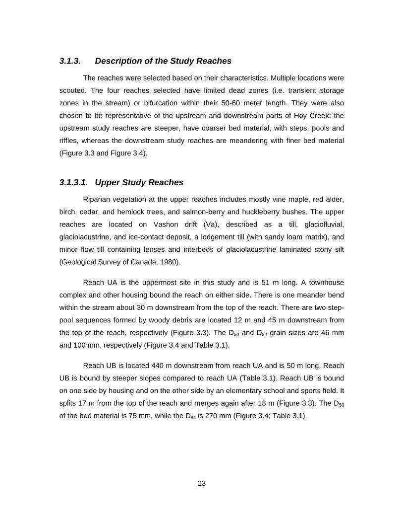
Figure 3.6 Precipitation and daily average temperature normals from 1971-2000 for Coquitlam and Port Moody, B.C. respectively (Environment Canada, 2010). ............................................................................................. 22

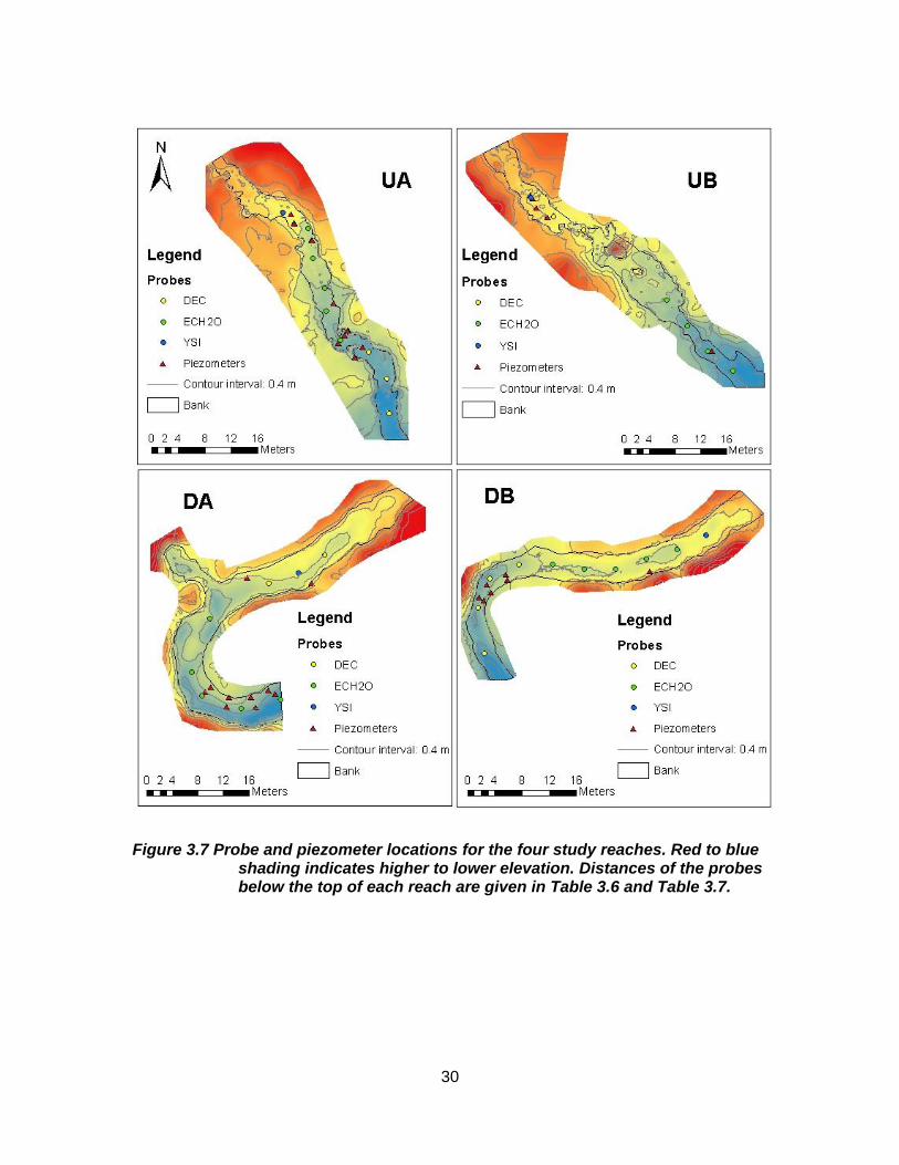
Figure 3.7 Probe and piezometer locations for the four study reaches. Red to blue shading indicates higher to lower elevation. Distances of the probes below the top of each reach are given in Table 3.6 and Table 3.7. ................................................................................................................ 30

Figure 3.8 Negative (left) and positive (right) VHG, indicating downwelling and upwelling hyporheic flow respectively (figure adapted from Baxter et al., 2003). ...................................................................................................... 35

Figure 3.9 Piezometer network across and around a meander bend in reach UA. ........ 36

Figure 4.1 Unexplained high discharge events (indicated by arrows). These streamflow responses were observed at the upper reach during periods without precipitation. ......................................................................... 42

Figure 4.2 Discharge (L/s) during the tracer experiments at reach UA. .......................... 46

Figure 4.3 Discharge (L/s) during the tracer experiments at reach UB. .......................... 47

Figure 4.4 Discharge (L/s) during the tracer experiments at reach DA. .......................... 48

xiv

Figure 4.5 Discharge (L/s) during the tracer experiments at reach DB. .......................... 49

Figure 4.6 Average rank of steady state EC for each reach. A high average rank indicates a relatively low steady state EC and thus a relatively high discharge. Refer to Figure 3.3 for an explanation of the features in the stream (different shades of blue represent riffles and pools). ....................... 50

Figure 4.7 Standard deviation (SD) of the rank of steady state EC at each probe location within each reach. A low SD indicates a more persistent rank, while a high SD indicates a highly variable rank for steady state EC. ........... 51

Figure 4.8 Vertical hydraulic gradients during the tracer experiments in reach UA. Negative values indicate downwelling. Positive values indicate upwelling. ...................................................................................................... 54

Figure 4.9 Vertical hydraulic gradient during the tracer experiments in reach UB. Negative values indicate downwelling. Positive values indicate upwelling. ...................................................................................................... 55

Figure 4.10 Vertical hydraulic gradient during the tracer experiments in reach DA. Negative values indicate downwelling. Positive values indicate upwelling. ...................................................................................................... 56

Figure 4.11 Vertical hydraulic gradient during the tracer experiments in reach DB. Negative values indicate downwelling. Positive values indicate upwelling. ...................................................................................................... 57

Figure 4.12 Average rank of the VHG for each reach. A low rank indicates a low (or more negative) VHG compared to the other sites in the reach, while a high rank indicates a relatively large positive VHG. .......................... 58

Figure 4.13 Standard deviation of the rank of the VHG in each reach. A low standard deviation of the rank indicates a persistent ranks. ......................... 59

Figure 4.14 Examples of the observed and modeled breakthrough curves at the YSI locations in the upper and lower reaches of Hoy Creek (UA and DB). Observed and modeled breakthrough curves of all experiments are provided in Appendix C. .......................................................................... 61

Figure 4.15 The time between the start of the increase in EC and steady state (rise to SS) divided by the time between the start of the experiment and the start of the increase in EC (start to rise) versus discharge (Q). Higher values of (rise to SS)/(Start to rise) indicate more transient storage and dispersion. The top figure shows the relation for the upper reaches and the bottom figure shows the relation for the lower reaches. ........................................................................................................ 66

xv

Figure 4.16 Relation between the optimized storage zone exchange coefficient (α) and discharge for the four reaches. Left column shows the data for the upper reaches (UA: filled symbols and UB: open symbols), the right columns show the data for the lower reaches (DA: filled symbols, DB: open symbols). The upper row shows the data for the YSI probe location, the bottom row for the ECH2O 5 probe location. ............................. 75

Figure 4.17 The optimized (filled symbols) and estimated cross-sectional area (open symbols) of the stream (A) for the upper reaches (top row) and lower reaches (bottom row) as a function of discharge. ................................ 76

Figure 4.18 The optimized storage zone cross-sectional area (As) for the upper reaches (left column) and lower reaches (right column) as a function of discharge for the YSI probe location (upper row) and ECH2O-5 location (lower row) (UA and DA: filled symbols and UB and DB: open symbols). ....................................................................................................... 77

Figure 4.19 The ratio of the cross-sectional area of the hyporheic zone and the cross-sectional area of the stream (As/A) as a function of discharge for the upstream reaches (left column) and downstream reaches (right column); YSI probe location (top row) and ECH2O-5 probe location (bottom row) (UA and DA: filled symbols and UB and DB: open symbols). ....................................................................................................... 79

Figure 4.20 Storage zone residence time as a function of discharge for the upper reaches (left column) and lower reaches (right column; UA and DA: filled symbols and UB and DB: open symbols). YSI probe location (top row) and ECH2O 5 probe location (bottom row). ........................................... 80

Figure 4.21 Hydraulic retention factor (Rh) as a function of discharge at the YSI probe location (UA and DA: filled symbols and UB and DB: open symbols). ....................................................................................................... 81

Figure 4.22 The average distance a water molecule travels in the stream before entering transient storage (Ls) as a function of discharge at the YSI probe location (top row) and ECH2O-5 location (bottom row) (UA and DA: filled symbols and UB and DB: open symbols). ..................................... 82

Figure 4.23 The Damköhler number (DaI) as a function of discharge for the tracer tests in the upper and lower reaches. The area between the dashed lines is the ideal range of DaI values. ........................................................... 83

Figure 4.24 Validation graphs for the tracer experiment on July 30, 2010 in reach DA. For the locations of the probes, see Figure 3.7. All other validation graphs are given in Appendix D. ................................................... 88

1

1. Introduction

1.1. Problem Statement

The hyporheic zone is a hydrologically, biologically, and chemically distinct area

between the stream and the surrounding streambed in which the exchange of water and

dissolved material occurs. It is preferred by salmon for spawning habitat, and acts as

natural filter for effluents, contaminants, and nutrients (Baxter and Hauer, 2000;

Hancock, 2002; Gandy et al., 2007). Additionally, hyporheic exchange increases the

degree of contact of subsurface water with the substrate and therefore increases the

solute residence time (Bencala, 2000). While the hyporheic zone is not frequently

significant in volume, it is significant for solute transport from the stream to the

subsurface (Bencala et al., 2011).

Harvey and Bencala (1993) conceptualize hyporheic flow as predominantly

horizontal flow outside of the stream and predominantly vertical flow beneath the stream

(Figure 1.1). Horizontal exchange of water occurs commonly through meander bends in

the stream. Longitudinal exchange occurs through step-pool and riffle-pool sequences in

a stream, which are associated with complexity of the streambed. Head gradients are

the driving force behind hyporheic exchange (Tonina and Buffington, 2009). The

composition of streambed material also affects movement of water through it, thereby

influencing the extent of the hyporheic zone and the amount of hyporheic exchange. For

example, coarser material results in a greater water exchange between the stream and

the hyporheic zone assuming there is a head gradient.

2

Figure 1.1 Vertical and lateral exchange of water between the open channel and the surrounding saturated sediments of the hyporheic zone (shaded area; adapted from Findlay, 1995).

A number of other factors also influence the extent of the hyporheic zone and the

rate of hyporheic exchange. These include discharge, streambed topography, and

channel planform (Harvey and Bencala, 1993; Harvey et al., 1996; Dahm et al., 2007).

However, previous studies have yielded inconsistent results regarding how discharge

influences the hyporheic zone and hyporheic exchange. Some studies have shown that

the hyporheic zone increases with increasing discharge (Wondzell, 2006; Patschke,

1999; Scordo and Moore, 2009), while others indicate a decrease with increasing

discharge (D’Angelo et al., 1993; Duineveld, 2008; Harvey et al., 1996). The same is

true for the rate of hyporheic exchange (Wondzell, 2006; Harvey et al., 1996; Karwan

and Saiers, 2009). Furthermore, some studies indicate no trend between the extent of

the hyporheic zone or then amount of hyporheic exchange and discharge (Legrand-

Marcq and Laudelout, 1985; Patschke, 1999; Scordo and Moore, 2009).

Despite an increase in the number of studies on hydrological processes within

the hyporheic zone, there is a need to continue to advance our knowledge of the

hyporheic zone. There is especially a need to compare results from different studies

(different flow rates, different streambed topographies, different streambed materials,

etc.) to derive generalities. According to Bencala (2000), “continuing advances in

knowledge of the hydrological processes in hyporheic zones are critical to quantitative

3

analysis of stream ecosystems”. Findlay (1995) states that there has been “no attempt to

uncover generalities across systems or to provide an organizing framework to simplify

intersystem comparisons”, which is in agreement with White (1993) who states, “to my

knowledge, a comparative examination of the hyporheic zones within any single, larger

river system (e.g., 1st order to 6th or larger order streams) has never been attempted”.

Krause et al. (2011a) add that one of the major issues with current and future research

of hyporheic exchange involves understanding scale dependencies and variability in

streambed properties. In addition, further research is needed on how hyporheic

exchange is influenced by discharge, streambed topography, and streambed material.

Research is also lacking regarding the hyporheic zone in urban streams; most

studies have been conducted under laboratory conditions or in forested areas. This

study therefore examines hyporheic exchange in an urban setting and compares it to

previous studies on hyporheic exchange in forested and laboratory settings.

1.2. Research Objectives

The objective of this project was to gain a better understanding of hyporheic

exchange in a suburban coastal British Columbia stream, and the factors that influence

it.

1.2.1. Research Questions

The specific research questions for this study were:

1. How different is hyporheic exchange in high and low gradient reaches?

2. How do hyporheic exchange and transient storage change with

discharge?

3. Can streambed topography and channel planform explain locations where

hyporheic exchange and lateral inflow occur?

4

1.2.2. Hypotheses

My hypotheses for this research were as follows:

Hypothesis 1: Hyporheic exchange will be greatest in high gradient reaches

and lowest in low gradient reaches due to decreasing head differences and finer

streambed sediment as a result of the lower stream velocities in the low gradient

reaches. The hyporheic zone will be larger in lower gradient reaches because the

stream is wider and streambed tends to be thicker in these areas.

Hypothesis 2: Hyporheic exchange will decrease with increasing discharge

because the influence of head differences due to obstructions decreases. However, the

extent of the hyporheic zone will increase with increasing discharge because the area

available for hyporheic exchange increases as the stream width widens, as found in

studies conducted in the Malcolm Knapp Research Forest in B.C. (Patschke, 1999;

Scordo and Moore, 2009).

Hypothesis 3: Streambed topographical features (specifically riffle and step-

pools), and channel planform (specifically meander bends) will be locations of increased

hyporheic exchange and lateral inflow during low flow conditions, but anthropogenic

features such as storm drains determine the locations of lateral inflows during high flow

conditions.

5

2. Literature Review

2.1. Introduction

Different scientific fields study the hyporheic zone and its implications for biotic

processes, filtration, and transformation of chemicals; as a result, a number of different

definitions of the hyporheic zone have been proposed. The term “hyporheic” is derived

from Greek, with “hypo” meaning “under”, and “rhe” meaning “flow” (Tonina and

Buffington, 2009).

Hydrologically the hyporheic zone can be defined as the zone in between the

stream and groundwater in which transient storage occurs. It can also be defined as the

saturated area that is affected by stream water, whereas groundwater is defined as the

saturated area unaffected by stream water (White, 1993). Harvey and Bencala (1993)

define the hyporheic zone as the subsurface area into which the downwelling

streamwater enters and is temporarily stored with the subsurface water already present

before re-entering the stream. The definition used in this study will be this hydrologically

relevant definition of the hyporheic zone, as this study will focus on the hydrological

aspects of the hyporheic zone rather than the biogeochemical and ecological aspects.

2.2. Significance of the Hyporheic Zone

The hyporheic zone is home to a diverse and unique set of organisms, especially

invertebrates, and is the site of significant biogeochemical activity (Marmonier et al.,

1993; Hancock, 2002). Different organisms inhabit the stream, groundwater, and

hyporheic zones. The aquatic invertebrates in the hyporheic zone are termed the

“hyporheos” and include crustaceans, water mites, worms, and juvenile stages of

aquatic insects (Boulton et al., 1998). Exchange of water from the stream to the

hyporheic zone changes stream water chemistry once water upwells from the hyporheic

6

zone. This is due to the anaerobic and aerobic metabolic processes, and a combination

of biogeochemical processes that occur in the hyporheic zone (Findlay, 1995). Dissolved

oxygen generally decreases within the hyporheic zone due to metabolic processes by

organisms that inhabit the hyporheic zone (Findlay, 1995). Additionally, due to retention

of water in the hyporheic zone, remineralization can delay the loss of nutrients (such as

nitrogen) from the stream, which can lead to increases in overall primary production

(Findlay, 1995).

The hyporheic zone has also been studied for its significance to fish, in particular,

salmon. Hyporheic exchange is more likely in areas characterized by gravels and a

complex streambed (ie. obstructions, step-pool and riffle-pool sequences), which is also

where salmon tend to spawn (Baxter and Hauer, 2000; Dauble and Geist, 2000;

Woessner, 2000; Hanrahan, 2008). Salmon and trout bury their eggs for incubation in

gravels in the hyporheic zone (Tonina and Buffington, 2009) because of the temperature

and porosity of the bed sediment. In winter, water is warmer due to hyporheic exchange

(assuming groundwater is warmer than stream water). This enhances incubation by

accelerating the growth and development of eggs (Hanrahan, 2008). Fish tend to inhabit

these areas in summer as well because of the upwelling of colder groundwater.

Additionally, when hyporheic exchange increases, the sediment becomes more

oxygenated due to advective flow, creating optimal conditions for embryos (Soulsby et

al., 2009; Tonino and Buffington, 2009).

The hyporheic zone can act as a natural filter for stream water. Hancock (2002)

identifies three main filtering mechanisms: physical, biological, and chemical. The

hyporheic zone acts as a physical filter by removing silt and particulate matter from

stream water that enters it. It acts as a biological filter by taking up or transforming

nutrients. The efficiency of this mechanism depends on the microbial activity in the

hyporheic zone. The hyporheic zone acts as a chemical filter by enabling chemical

reactions, such as redox processes and metal precipitation, to occur. This depends on

the chemical conditions within the hyporheic zone. Hyporheic retention and subsequent

remineralization can delay the loss of nutrients from a stream reach and thus influence

stream nutrient budgets (Findlay, 1995).

7

2.3. Controls on Hyporheic Exchange

Streambed composition and porosity, channel topography, topography of the

surrounding area, and discharge all determine the extent of the hyporheic zone (Harvey

and Bencala, 1993; Harvey et al., 1996; Hancock, 2002; Dahm et al., 2007). This

literature review will give an overview of the results of previous studies conducted on the

influences on hyporheic exchange.

2.3.1. Discharge

Many studies have found that discharge affects hyporheic exchange. However,

the results are inconsistent (Table 2.1 and Table 2.2); some studies indicated that

hyporheic exchange increases with increasing discharge, while others found the

opposite. Wondzell (2011) showed that hyporheic exchange is greater in smaller

streams compared to larger streams, because in larger streams with greater discharge,

the processes driving the exchange become hydrologically constrained. Ryan et al.

(2010) investigated the effects of riparian land cover on the hyporheic zone at various

discharge levels in a third order urban stream in Maryland and found that exchange

between the stream and groundwater was greater during summer baseflow than during

spring; they also found that less riparian forest cover resulted in a greater influence of

discharge on the exchange and transient storage due to the effects of vegetation within

the stream. Hart et al. (1999) speculate that the small size of the hyporheic zone in their

study site was the reason that they did not find evidence of a trend in the change of the

hyporheic zone with increasing discharge.. Another suggested explanation for the

variations in study results is that streams have different morphologies, and solute

exchange may not scale with discharge in the same way for each stream (Schmid et al.,

2010). D’Angelo et al. (1993) hypothesized that increased hyporheic exchange with

increased discharge may be the result of the increased availability of the solute over

time, and flushing of hyporheic exchange site when discharge is high. They also gave

two explanations for why the hyporheic zone decreased with increased discharge. The

first is decreased channel complexity between headwaters and downstream sites, which

results in a smaller transient storage area due to the elimination of potential transient

storage zones that could have formed behind these features. The second explanation is

8

Table 2.1 Overview of studies on the influence of discharge on the size of the hyporheic zone (HZ).

9

Table 2.2 Overview of studies on the influence of discharge on hyporheic exchange (HE).

that transient storage zones act more independently during low discharge periods

compared to high flow periods when transient storage zones might be incorporated into

the stream. More data are needed to determine if these explanations are correct.

More studies need to be conducted on the size of the hyporheic zone during

storms and over a longer period to determine the degree of hyporheic and surface water

interaction. Boano et al. (2010) showed that mean discharge can be used to estimate

the average properties of hyporheic exchange under unsteady conditions. Additionally,

10

discharge fluctuations were found to cause variations in the rate of exchange and

subsurface residence time distributions. Maier and Howard (2011) found that stream-

stage fluctuations increased the rate and amount of groundwater-stream water mixing,

increased the depth that particles penetrate into the streambed, and increased the size

of the hyporheic zone.

2.3.2. Geomorphic Features

The amount of horizontal and longitudinal exchange depends on the extent of the

hyporheic zone and the composition of the streambed material. Areas confined by

hillslopes consisting mainly of bedrock with low hydraulic conductivity have small

hyporheic zones, whereas areas on a floodplain with high conductivity alluvial sediments

have large hyporheic zones (Tonina and Buffington, 2009). The following key factors

control vertical and lateral hyporheic exchange in the alluvial zone: (a) hydraulic

conductivity of the alluvium, (b) hydraulic gradient between either end of the riffle, and

(c) the influx of groundwater to the alluvium from its surroundings (Storey et al., 2003).

Most studies that have investigated the influence of geomorphic features (step-

pool and riffle-pool sequences, meanders, obstructions) on hyporheic exchange have

found that when the stream is more complex, hyporheic exchange is enhanced,

depending on the hydraulic conductivity of the streambed (Gooseff et al., 2007). Large

woody debris can increase hyporheic exchange by increasing complexity and enhancing

vertical connectivity in the stream (Sawyer et al., 2012). Tonina and Buffington (2007)

showed that hyporheic exchange is the result of a complex interaction between

discharge and bedform topography. Jones et al. (2008) found that features such as side

channels, backwaters, tributaries, and springs outside the stream channel were also

critical drivers of hyporheic flow. Baxter and Hauer (2000) and Kasahara and Wondzell

(2003) showed that channel morphology (stream size and channel constraint) controlled

hyporheic exchange. Lautz et al. (2010) described three scenarios where hyporheic

exchange occurs: upstream of an impoundment, rapid flow through shallow hyporheic

flow cells, and rapid downwelling through riffles. The topography of the valley floor

controls the development of the flow system, which in turn predicts the location and

extent of the hyporheic zone (Wondzell and Swanson, 1996). Krause et al. (2011b)

found that the vertical hydraulic gradient (VHG) is affected by high pressure at different

11

points along a riffle-pool system due to obstacles on the streambed: surface water

infiltrates into the pore space of the bed upstream of the obstacle, and exfiltrates

downstream of the obstacle, suggesting that streambed topography significantly

influences the exchange of water between the stream and the subsurface. Wondzell

(2011) found that hyporheic exchange is smaller in low gradient streams in comparison

to high gradient streams.

Examining hyporheic exchange requires knowledge of the streambed topography

as the depth and spatial pattern of hyporheic exchange are controlled by the amplitude

and wavelength of the head surface along the streambed (Tonina and Buffington, 2007).

An obstruction may create a high pressure zone upstream that can drive hyporheic

exchange and circulation (Tonina and Buffington, 2007). In general, if the curvature of

the streambed is concave, upwelling from the hyporheic zone occurs; if the curvature is

convex, downwelling into the hyporheic zone occurs (Tonina and Buffington, 2007). This

correlates to riffle and pool systems in that the convex riffle portion of the stream is a

downwelling area, and the concave pool portion of the stream is an upwelling area

(Kasahara and Hill, 2008). Other structures like large wood and debris dams, large

boulders, and pool and boulder steps, function in this manner as well (Harvey and

Bencala, 1993; Stofleth et al., 2008; Lautz et al., 2010). If depth of alluvium is not

limiting, high amplitude and long wavelength head variations will result in deeper

hyporheic flow compared with areas of limited alluvium (smaller depth to bedrock or

other layer with a very low conductivity) (Kasahara and Wondzell, 2003; Tonina and

Buffington, 2009). Shorter wavelength/amplitude head variations create more circulation

cells with reduced path lengths and exchange times (Tonina and Buffington, 2009). More

complex streambed topography and variation in bed material can lead to more variable

residence time distributions as well as smaller streambed fluxes (Ward et al., 2012).

Horizontal features, such as meander bends and gravel bars are also areas of

enhanced hyporheic exchange (Harvey and Bencala, 1993; Wroblicky et al., 1998;

Kasahara and Hill, 2007; Cardenas, 2008; Takahashi et al., 2008). Takahashi et al.

(2008), for example, found that strong preferential flow through the hyporheic zone

occurred across meander bends. However, Harvey and Bencala (1993) found that while

hyporheic flow occurred across a meander bend due to the curvature of the stream, it

was less pronounced in comparison to hyporheic flow driven by streambed topography.

12

2.3.3. Lateral Inflow and Hillslope Topography

Lateral inflow includes water contribution to the stream from groundwater,

overland flow, interflow, or small springs (Runkel, 1998). Few studies have investigated

lateral inflow into streams. Beven (2006) stated “we need more studies of the

incremental discharge into stream channels, so that we are encouraged to explore the

reasons for the heterogeneity of inputs”. Some studies suggest that topography

determines the location of lateral inflow to streams. Lateral inflows can be expected to

be a function of stream topography, substrate and stream bank porosity, total sub-

surface water volume and flow, as well as water table height (D’Angelo et al., 1993).

D’Angelo et al. (1993) found that lateral inflow was greatest in larger streams, but

speculated that its importance in regulating temperature and nutrient concentrations in

the stream may be greater in small streams, especially during low flows.

Different topographic features, such as spurs and hollows, result in different

wetness conditions, and therefore may be associated with different relative runoff

amounts (Anderson and Burt, 1978). Due to convergence of hydrologic flowpaths,

hollows were wetter, which led to more runoff in comparison to spurs amounts in the

study of Anderson and Burt (1978). Huff et al. (1982) also found that topography had a

significant influence on lateral inflow to streams. Their results indicated that significant

inflow occurred just opposite of a hollow, supporting the idea that hollows contribute

more subsurface flow to the stream in comparison to spurs or planar slopes. In addition,

Huff et al. (1982) found that the underlying bedding planes of the bedrock also affect

subsurface flow by providing a lateral flowpath along the strike towards the stream

channel. Fractures and dikes may provide a means of lateral transport of water to the

stream channel and may control the locations of lateral inflow.

In an urban stream, culverts and other drainage structures may have a greater

influence on lateral inflow compared to lateral inflow of subsurface flow from hillslopes

and groundwater, especially during rain events. Impervious surfaces, such as streets,

direct runoff into the stream via culverts and other drainage structures, and therefore

may have a greater influence on streamflow during rainfall conditions compared to

natural lateral inflows from the riparian zone surrounding the stream (Paul and Meyer,

2001; Wheeler et al., 2005). As a watershed becomes more urbanized, peak streamflow

13

volume also increases, indicating that lateral inflow due to drainage networks that feed

directly into the stream may be more prominent and efficient in routing rainfall to the

stream than hillslope and groundwater inflows (Wheeler et al., 2005).

2.4. Transport Processes and Modeling Hyporheic Exchange

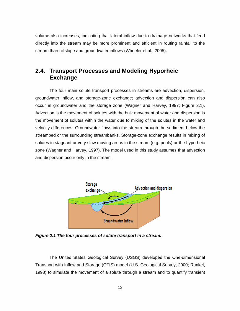
The four main solute transport processes in streams are advection, dispersion,

groundwater inflow, and storage-zone exchange; advection and dispersion can also

occur in groundwater and the storage zone (Wagner and Harvey, 1997; Figure 2.1).

Advection is the movement of solutes with the bulk movement of water and dispersion is

the movement of solutes within the water due to mixing of the solutes in the water and

velocity differences. Groundwater flows into the stream through the sediment below the

streambed or the surrounding streambanks. Storage-zone exchange results in mixing of

solutes in stagnant or very slow moving areas in the stream (e.g. pools) or the hyporheic

zone (Wagner and Harvey, 1997). The model used in this study assumes that advection

and dispersion occur only in the stream.

Figure 2.1 The four processes of solute transport in a stream.

The United States Geological Survey (USGS) developed the One-dimensional

Transport with Inflow and Storage (OTIS) model (U.S. Geological Survey, 2000; Runkel,

1998) to simulate the movement of a solute through a stream and to quantify transient

14

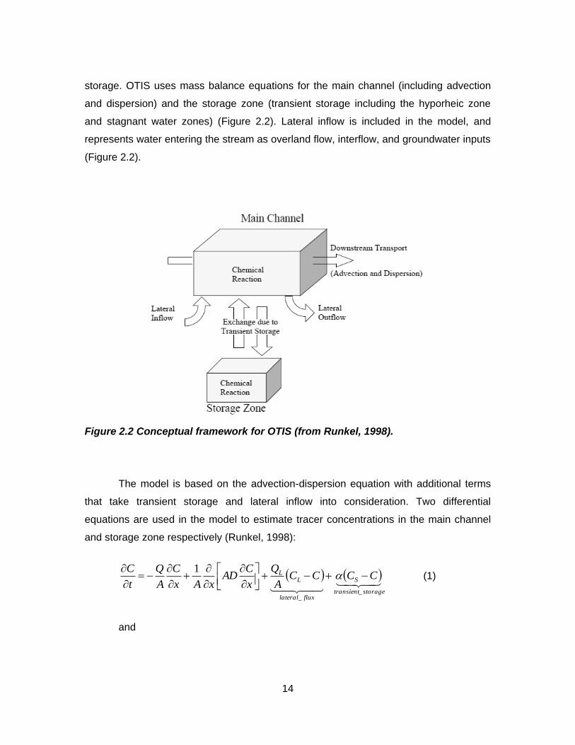
storage. OTIS uses mass balance equations for the main channel (including advection

and dispersion) and the storage zone (transient storage including the hyporheic zone

and stagnant water zones) (Figure 2.2). Lateral inflow is included in the model, and

represents water entering the stream as overland flow, interflow, and groundwater inputs

(Figure 2.2).

Figure 2.2 Conceptual framework for OTIS (from Runkel, 1998).

The model is based on the advection-dispersion equation with additional terms

that take transient storage and lateral inflow into consideration. Two differential

equations are used in the model to estimate tracer concentrations in the main channel

and storage zone respectively (Runkel, 1998):

storagetransient

S

fluxlateral

LL CCCC

A

Q

x

CAD

xAx

C

A

Q

t

C

__

1

(1)

and

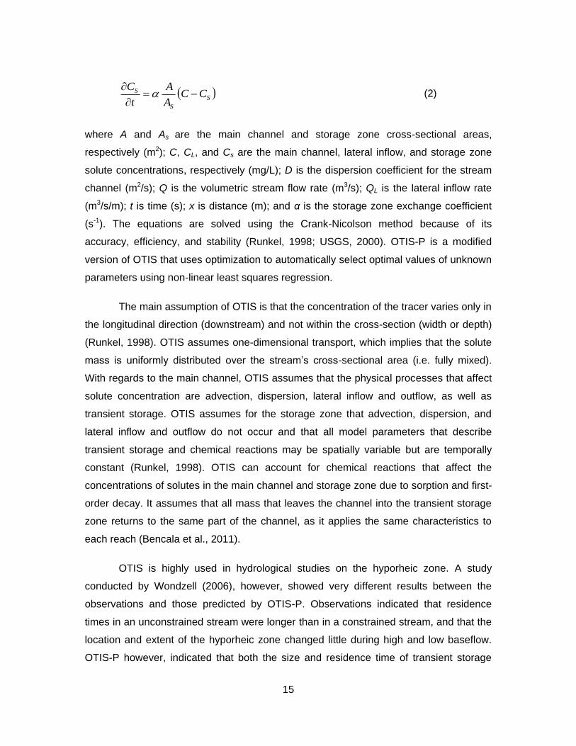
15

S

S

S CCA

A

t

C

(2)

where A and As are the main channel and storage zone cross-sectional areas,

respectively (m2); C, CL, and Cs are the main channel, lateral inflow, and storage zone

solute concentrations, respectively (mg/L); D is the dispersion coefficient for the stream

channel (m2/s); Q is the volumetric stream flow rate (m3/s); QL is the lateral inflow rate

(m3/s/m); t is time (s); x is distance (m); and α is the storage zone exchange coefficient

(s-1). The equations are solved using the Crank-Nicolson method because of its

accuracy, efficiency, and stability (Runkel, 1998; USGS, 2000). OTIS-P is a modified

version of OTIS that uses optimization to automatically select optimal values of unknown

parameters using non-linear least squares regression.

The main assumption of OTIS is that the concentration of the tracer varies only in

the longitudinal direction (downstream) and not within the cross-section (width or depth)

(Runkel, 1998). OTIS assumes one-dimensional transport, which implies that the solute

mass is uniformly distributed over the stream’s cross-sectional area (i.e. fully mixed).

With regards to the main channel, OTIS assumes that the physical processes that affect

solute concentration are advection, dispersion, lateral inflow and outflow, as well as

transient storage. OTIS assumes for the storage zone that advection, dispersion, and

lateral inflow and outflow do not occur and that all model parameters that describe

transient storage and chemical reactions may be spatially variable but are temporally

constant (Runkel, 1998). OTIS can account for chemical reactions that affect the

concentrations of solutes in the main channel and storage zone due to sorption and first-

order decay. It assumes that all mass that leaves the channel into the transient storage

zone returns to the same part of the channel, as it applies the same characteristics to

each reach (Bencala et al., 2011).

OTIS is highly used in hydrological studies on the hyporheic zone. A study

conducted by Wondzell (2006), however, showed very different results between the

observations and those predicted by OTIS-P. Observations indicated that residence

times in an unconstrained stream were longer than in a constrained stream, and that the

location and extent of the hyporheic zone changed little during high and low baseflow.

OTIS-P however, indicated that both the size and residence time of transient storage

16

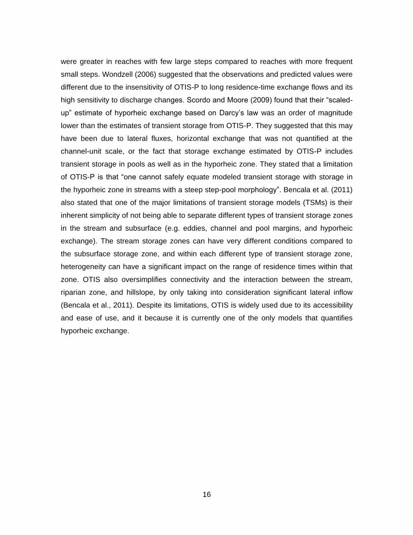
were greater in reaches with few large steps compared to reaches with more frequent

small steps. Wondzell (2006) suggested that the observations and predicted values were

different due to the insensitivity of OTIS-P to long residence-time exchange flows and its

high sensitivity to discharge changes. Scordo and Moore (2009) found that their “scaled-

up” estimate of hyporheic exchange based on Darcy’s law was an order of magnitude

lower than the estimates of transient storage from OTIS-P. They suggested that this may

have been due to lateral fluxes, horizontal exchange that was not quantified at the

channel-unit scale, or the fact that storage exchange estimated by OTIS-P includes

transient storage in pools as well as in the hyporheic zone. They stated that a limitation

of OTIS-P is that “one cannot safely equate modeled transient storage with storage in

the hyporheic zone in streams with a steep step-pool morphology”. Bencala et al. (2011)

also stated that one of the major limitations of transient storage models (TSMs) is their

inherent simplicity of not being able to separate different types of transient storage zones

in the stream and subsurface (e.g. eddies, channel and pool margins, and hyporheic

exchange). The stream storage zones can have very different conditions compared to

the subsurface storage zone, and within each different type of transient storage zone,

heterogeneity can have a significant impact on the range of residence times within that

zone. OTIS also oversimplifies connectivity and the interaction between the stream,

riparian zone, and hillslope, by only taking into consideration significant lateral inflow

(Bencala et al., 2011). Despite its limitations, OTIS is widely used due to its accessibility

and ease of use, and it because it is currently one of the only models that quantifies

hyporheic exchange.

17

3. Study Site and Methodology

3.1. Study Site

3.1.1. Hoy Creek, Coquitlam

This research took place in Hoy Creek in Coquitlam, B.C. (Figure 3.1). The two

research sites are located within an urban setting: one in an upstream, steeper portion of

Hoy Creek and one in a downstream, meandering portion. The upper part of Hoy Creek

is located at about 270 m. asl, and the lower part of Hoy Creek at about 40 m. asl (data

from the World Geodetic System of 1984 datum and Earth Gravitational Model 1996

Geoid). Each study area consisted of two study reaches. Studying multiple reaches of

the same stream increases the statistical power compared to studying the stream as a

whole and is also more practical.

Hoy Creek provides an interesting study location for studying hyporheic

exchange in a suburban stream as it is a known salmon spawning stream with a fish

hatchery. Streams with considerable hyporheic exchange are preferred by salmon for

spawning (Baxter and Hauer, 2000). All studied reaches are fish-bearing reaches

(CH2M Hill, 2012). The Hoy Scott Watershed Society maintains Hoy Creek (Houghton,

2008).

Hoy Creek is bordered on both sides by housing. It originates in North Hoy Creek

near the top of Westwood Plateau in Coquitlam and flows southward into Scott Creek, a

tributary of the Coquitlam River. Due to urban development in the Lower Coquitlam River

Watershed and around Hoy Creek, a significant portion of the watershed’s drainage is

carried through the storm drain system. Numerous culverts direct flow into the creek. In

1999, 20.8% of the watershed area of Hoy Creek was effectively impermeable (Fraser

River Action Plan, 1999). In 2005, the Scott-Hoy Creek Watershed had a total

impervious area (TIA) of 40%, and a riparian forest integrity (RFI) of 40% (CH2M Hill,

18

2012). All four study reaches are classified as having medium compaction (CH2M Hill,

2012). RFI values given in the Scott Creek Integrated Watershed Management Plan

(CH2M Hill, 2012) were 75% from Parkway Boulevard to Camelback Court (Reach UA),

100% from Camelback Court to Plateau Boulevard (Reach UB), and 39% from David

Avenue to Guildford Way (Reaches DA and DB). Comparison of calculated TIA values

from 1996 and 2005 indicate that the Scott Creek Watershed, which includes Hoy Creek,

has declined from fair to poor health due to the effects of urbanization (i.e. loss of

riparian forest habitat). This is more notable in the lower portion of Hoy Creek than the

upper portion since more development has occurred in the upper watershed since 1999.

The upper portion of Hoy Creek is quite different in comparison to the lower

portion (Figure 3.2, Figure 3.3, and Table 3.1). The upper part has a considerably larger

amount of woody debris. Steeper forested slopes surround it, and it has a coarser

grained streambed compared to the downstream reaches of Hoy Creek (Figure 3.4 and

Table 3.1). The lower part of Hoy Creek is located on Capilano sediments of glacial

gravel and sand, while the upper part is located on Vashon drift of glacial till (Geological

Survey of Canada, 1997). Discharge is lower in the upper reaches of Hoy Creek

compared to the lower reaches (Figure 3.5 and Table 3.1).

Table 3.1 Upper (UA and UB) and lower (DA and DB) reach characteristics.

Characteristic UA UB DA DB

D50 (mm) 4.6 7.5 3.9 4.0

D84 (mm) 10.0 27.0 7.0 7.6

Length (m) 51.2 49.7 62.8 54.7

Stream slope (%) 31.2 38.7 20.7 18.6

Near-stream hillslope (%) 7 8 3 5

Watershed hillslope (%) 13 23 6 5

Average channel width (m) 2.5 3.1 4.5 4.0

Average discharge (Jul-Sept 2010) (L/s) 3.3 9.7 30.1 53.0

Average discharge (Jul-Sept 2010) (mm/day) 0.6 1.5 0.7 1.3

Average discharge (Oct-Dec 2010) (L/s) 25.7 30.1 279.8 104.0

Average discharge (Oct-Dec 2010) (mm/day) 4.7 4.7 7.2 2.3

19

Figure 3.1 Location of Hoy Creek in Coquitlam, BC. (Data source: Google Earth, Digital Globe, accessed June 8, 2012)

Figure 3.2 Photos of the upper (left two images) and lower (right two images) reaches of Hoy Creek during low flow conditions.

20

Figure 3.3 Main features in the upper and lower study reaches of Hoy Creek and locations of the piezometers. The trees that are labelled have a significant influence on the stream since they protrude into the flow.

21

Figure 3.4 Cumulative frequency of the B-axis of bed material based on a Wolman pebble counts for reaches UA, UB, DA, and DB.

Figure 3.5 Precipitation and discharge in upper and lower Hoy Creek.

22

3.1.2. Climate and Streamflow Normals

Hoy Creek is located within the Coastal Western Hemlock biogeoclimatic zone

(Pojar et al.,1991). Average annual precipitation for Coquitlam is 1859 mm (Environment

Canada, 2010). The months of June to August are relatively dry with average

precipitation ranging from 62-92 mm/month; October to January is wet, with average

precipitation ranging between 182-299 mm/month (Figure 3.6). Average monthly

temperature data for Coquitlam was unavailable, but the data for the neighbouring

community of Port Moody, which is located 4 km west of Hoy Creek, was used instead

(Figure 3.6). The average daily temperature in Port Moody ranged between 3-10.5°C

between October and January, and between 14.8-17.8°C between June to September

(Environment Canada, 2010).

Figure 3.6 Precipitation and daily average temperature normals from 1971-2000 for Coquitlam and Port Moody, B.C. respectively (Environment Canada, 2010).

23

3.1.3. Description of the Study Reaches

The reaches were selected based on their characteristics. Multiple locations were

scouted. The four reaches selected have limited dead zones (i.e. transient storage

zones in the stream) or bifurcation within their 50-60 meter length. They were also

chosen to be representative of the upstream and downstream parts of Hoy Creek: the

upstream study reaches are steeper, have coarser bed material, with steps, pools and

riffles, whereas the downstream study reaches are meandering with finer bed material

(Figure 3.3 and Figure 3.4).

3.1.3.1. Upper Study Reaches

Riparian vegetation at the upper reaches includes mostly vine maple, red alder,

birch, cedar, and hemlock trees, and salmon-berry and huckleberry bushes. The upper

reaches are located on Vashon drift (Va), described as a till, glaciofluvial,

glaciolacustrine, and ice-contact deposit, a lodgement till (with sandy loam matrix), and

minor flow till containing lenses and interbeds of glaciolacustrine laminated stony silt

(Geological Survey of Canada, 1980).

Reach UA is the uppermost site in this study and is 51 m long. A townhouse

complex and other housing bound the reach on either side. There is one meander bend

within the stream about 30 m downstream from the top of the reach. There are two step-

pool sequences formed by woody debris are located 12 m and 45 m downstream from

the top of the reach, respectively (Figure 3.3). The D50 and D84 grain sizes are 46 mm

and 100 mm, respectively (Figure 3.4 and Table 3.1).

Reach UB is located 440 m downstream from reach UA and is 50 m long. Reach

UB is bound by steeper slopes compared to reach UA (Table 3.1). Reach UB is bound

on one side by housing and on the other side by an elementary school and sports field. It

splits 17 m from the top of the reach and merges again after 18 m (Figure 3.3). The D50

of the bed material is 75 mm, while the D84 is 270 mm (Figure 3.4; Table 3.1).

24

3.1.3.2. Lower Study Reaches

Riparian vegetation at the lower reaches includes numerous tree species (cedar,

hemlock, red alder, birch, broadleaf maple, and vine maple), salmon-berry, huckleberry,

salal, and blackberry bushes. Reach DB is located in a stretch of Hoy Creek identified as

having a major invasive species intrusion of mainly Himalayan blackberry and Japanese

knotweed (CH2M Hill, 2012). Reach DA has been identified as a site of severe erosion

defined with an area of more than 10 m2 (CH2M Hill, 2012). Reaches DA and DB are

both located downstream of a wetland area. According to the Geological Survey of

Canada mapping (1980), these lower reaches are located on Capilano sediments (Cc),

described as a raised deltaic and channel till with medium sand to cobble gravel up to 15

m thick deposited by proglacial streams, which is in most places underlain by silty to silty

clay loam.

Reach DA is the uppermost of the two downstream reaches. A bridge crosses

the stream just upstream from the top of the reach, which is located about half way

around a meander bend. There is another meander bend towards the end of the reach.

Two culverts enter the stream in this reach, one near the top of the reach and another

about half-way down the reach (Figure 3.3). One side of the stream is bordered by a

high school and a post-secondary school, while a townhouse complex is located on the

opposite side. The D50 of the bed material is 39 mm, while the D84 is 70 mm Figure 3.4).

Reach DB is the furthest downstream study reach in Hoy Creek. A townhouse

complex and a well-used gravel trail border one side of the stream, while the other side

contains a riparian buffer zone of smaller shrubs and trees, approximately 80 m wide.

This reach contains one meander bend near the downstream end of the reach (Figure

3.3). The D50 of the bed material is 40 mm; the D84 is 75 mm (Figure 3.4).

25

3.2. Methodology

3.2.1. Tracer Experiments

Steady state tracer experiments were used to characterise the movement of

water through the stream and hyporheic zone. Tracer experiments are a common

method to assist in determining where and how fast water is flowing. Steady state (i.e.

constant injection) tracer experiments are more reliable than slug injections because the

rising and falling limb data from slug injections are cumulatively less informative than

those of steady state injections, thereby influencing the estimate of the lateral volumetric

groundwater inflow rate (Wagner and Harvey, 1997).The tracer experiments were

conducted during low and high discharge conditions. The low discharge period lasted

from June to mid-September 2010, and the high discharge period from mid-September

to December 2010 (Figure 3.5). In total 40 tracer tests were conducted, 10 in each

reach. Experiments were conducted in a random order, based on the time available for

the experiment and rotation of sites (Table 3.2-Table 3.5).

Sodium chloride, a conservative solute tracer, was injected into the stream at

each of the reaches until steady state electrical conductivity (EC) was reached at the

downstream end of the reach. According to the Canadian Water Quality Guidelines

(Nagpal et al., 2003), the concentration of sodium chloride should not exceed 150 mg/L

to protect freshwater aquatic life from chronic effects. To ensure protection of freshwater

aquatic life from acute and lethal effects, the Canadian Water Guidelines suggest that

the concentration of sodium chloride should not exceed 600 mg/L at any time. The

maximum increase in concentration of sodium chloride in the stream during an

experiment was 87 mg/L. For one test the sodium chloride increased to a maximum

concentration of 240 mg/L for 3 hours, and for three tests it increased to a maximum

concentration between 170-185 mg/L for 1-2 hours, all of which are well below the

maximum allowable concentration of sodium chloride for protection against acute and

lethal effects. The maximum concentrations during the other tests were below 150 mg/L

(Table 3.2-Table 3.5). The concentration of the injected tracer solution required for the

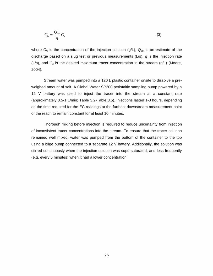
tracer tests was determined using the equation:

26

sest

is Cq

QC (3)

where Cis is the concentration of the injection solution (g/L), Qest is an estimate of the

discharge based on a slug test or previous measurements (L/s), q is the injection rate

(L/s), and Cs is the desired maximum tracer concentration in the stream (g/L) (Moore,

2004).

Stream water was pumped into a 120 L plastic container onsite to dissolve a pre-

weighed amount of salt. A Global Water SP200 peristaltic sampling pump powered by a

12 V battery was used to inject the tracer into the stream at a constant rate

(approximately 0.5-1 L/min; Table 3.2-Table 3.5). Injections lasted 1-3 hours, depending

on the time required for the EC readings at the furthest downstream measurement point

of the reach to remain constant for at least 10 minutes.

Thorough mixing before injection is required to reduce uncertainty from injection

of inconsistent tracer concentrations into the stream. To ensure that the tracer solution

remained well mixed, water was pumped from the bottom of the container to the top

using a bilge pump connected to a separate 12 V battery. Additionally, the solution was

stirred continuously when the injection solution was supersaturated, and less frequently

(e.g. every 5 minutes) when it had a lower concentration.

27

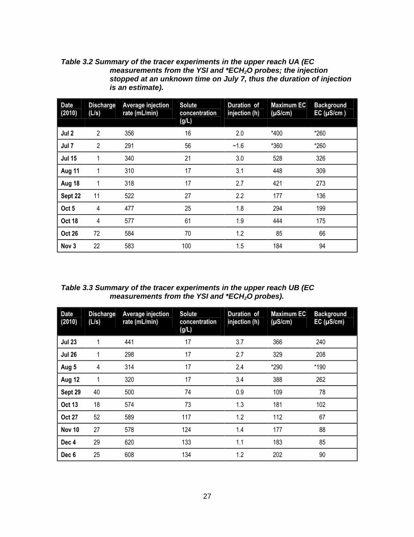
Table 3.2 Summary of the tracer experiments in the upper reach UA (EC measurements from the YSI and *ECH2O probes; the injection stopped at an unknown time on July 7, thus the duration of injection is an estimate).

Date (2010)

Discharge (L/s)

Average injection rate (mL/min)

Solute concentration (g/L)

Duration of injection (h)

Maximum EC (µS/cm)

Background EC (µS/cm )

Jul 2 2 356 16 2.0 *400 *260

Jul 7 2 291 56 ~1.6 *360 *260

Jul 15 1 340 21 3.0 528 326

Aug 11 1 310 17 3.1 448 309

Aug 18 1 318 17 2.7 421 273

Sept 22 11 522 27 2.2 177 136

Oct 5 4 477 25 1.8 294 199

Oct 18 4 577 61 1.9 444 175

Oct 26 72 584 70 1.2 85 66

Nov 3 22 583 100 1.5 184 94

Table 3.3 Summary of the tracer experiments in the upper reach UB (EC measurements from the YSI and *ECH2O probes).

Date (2010)

Discharge (L/s)

Average injection rate (mL/min)

Solute concentration (g/L)

Duration of injection (h)

Maximum EC (µS/cm)

Background EC (µS/cm)

Jul 23 1 441 17 3.7 366 240

Jul 26 1 298 17 2.7 329 208

Aug 5 4 314 17 2.4 *290 *190

Aug 12 1 320 17 3.4 388 262

Sept 29 40 500 74 0.9 109 78

Oct 13 18 574 73 1.3 181 102

Oct 27 52 589 117 1.2 112 67

Nov 10 27 578 124 1.4 177 88

Dec 4 29 620 133 1.1 183 85

Dec 6 25 608 134 1.2 202 90

28

Table 3.4 Summary of the tracer experiments in the lower reach DA (EC measurements from the YSI and *ECH2O probes).

Date (2010)

Discharge (L/s)

Average injection rate (mL/min)

Solute concentration (g/L)

Duration of injection (h)

Maximum EC (µS/cm)

Background EC (µS/cm)

Jul 14 46 333 73 2.1 171 153

Jul 22 36 559 76 1.7 185 145

Jul 30 23 579 89 2.0 234 157

Aug 6 27 554 75 2.3 223 158

Aug 10 26 499 73 3.0 215 167

Aug 19 19 556 87 1.8 247 159

Sept 15 40 592 97 1.9 209 161

Sept 28 335* 717 281 0.9 100 87

Oct 19 49 733 185 1.2 237 144

Nov 9 233 600 356 1.3 150 118

Nov 16 266* 658 366 1.4 104 88

Table 3.5 Summary of the tracer experiments in the lower reach DB (EC measurements from the YSI and *ECH2O probes).

Date (2010)

Discharge (L/s)

Average injection rate (mL/min)

Solute concentration (g/L)

Duration of injection (h)

Maximum EC (µS/cm)

Background EC (µS/cm)

Jul 20 23 588 62 2.0 215 160

Jul 27 21 552 64 2.4 211 154

Aug 4 23* 583 83 2.4 *230 *160

Aug 16 25 537 86 2.4 221 158

Sept 24 144 728 169 0.9 132 103

Oct 12 114 658 151 1.3 137 110

Oct 20 64 732 159 1.3 217 155

Oct 29 61 656 290 1.2 212 107

Nov 12 83 654 382 1.1 224 122

Dec 3 158 708 374 1.1 175 118

29

The electrical conductivity (EC) was measured at multiple locations along the

reach (about every 5 m) using five ECH2O-TE probes, one YSI 6920-V2 EC probe, and

five homemade EC and temperature probes that are similar in design to the Campbell

Scientific CS547A probes (Figure 3.7). The ECH2O probes are named ECH2O 1- ECH2O

5 hereafter, with the ECH2O 1 probe always being located furthest upstream. The YSI

6920-V2 EC probe is named YSI and the homemade probes are named DEC 1-DEC 5

hereafter.

Brilliant blue dye was injected into the stream at the upstream end of each reach

to assess whether there was sufficient mixing in the stream and to determine where the

first measurement site could be located. Distances between probe locations are

provided in Table 3.6 and Table 3.7. Once steady state was reached, EC and

temperature measurements were taken approximately every 5 meters throughout the

reach using a Hanna pH/EC/TDS/Temperature probe (resulting in about 10

measurements in each reach). These measurements were used to determine where

lateral inflow might occur because the tracer becomes more diluted where lateral inflow

occurs and were mapped in ArcGIS and used to determine the locations of lateral inflow.

Lateral outflow is more difficult to determine as the tracer method is insensitive to losses

from the stream because the water leaving the stream does not change the

concentration of tracer within the stream (Bencala et al., 2011).

EC measurements were converted to concentration values (g/L of salt) by

calibrating the probes in the lab using water from Hoy Creek. R2 values of the dilution

standard were good for the ECH2O and YSI probes, and a bit lower for the DEC probes

(Table 3.8). The EC data collected during the tracer tests were used to create

breakthrough curves.

30

Figure 3.7 Probe and piezometer locations for the four study reaches. Red to blue shading indicates higher to lower elevation. Distances of the probes below the top of each reach are given in Table 3.6 and Table 3.7.

31

Table 3.6 Distance of each probe from the injection site for the upper reaches.

Reach UA Reach UB

Probe Distance from injection site (m) Probe Distance from injection site (m)

YSI 12.0 YSI 7.2

ECH2O 1 15.7 DEC 1 11.7

ECH2O 2 20.7 DEC 3 16.7

ECH2O 3 25.7 ECH2O 1 34.7

ECH2O 4 30.7 ECH2O 2 39.7

ECH2O 5 35.7 ECH2O 3 44.7

DEC 3 41.7 ECH2O 4/5 49.7

DEC 5 46.2

DEC 4 51.2

Table 3.7 Distance of each probe from the injection site for the lower reaches.

Reach DA Reach DB

Probe Distance from injection site (m) Probe Distance from injection site (m)

DEC 1 18.0 YSI 7.7

YSI 23.0 ECH2O 1 12.7

DEC 2/3 28.0 ECH2O 2 17.7

ECH2O 1 33.8 ECH2O 3 22.7

ECH2O 2 48.8 ECH2O 4 27.7

ECH2O 3 52.8 ECH2O 5 32.7

ECH2O 4 57.8 DEC 1 37.7

ECH2O 5 62.8 DEC 5 42.7

DEC 3 47.7

DEC 4 54.7

32

Table 3.8 R2 values for the relation between EC (x) and concentration of NaCl (y) for the eleven probes used in this study.

Probe Equation R2

YSI y = 0.0005x -0.0391 0.99993

ECH2O 1 y = 0.5031x-0.0369 0.99990

ECH2O 2 y = 0.4901x-0.0405 0.99981

ECH2O 3 y = 0.4922x-0.0413 0.99943

ECH2O 4 y = 0.4935x-0.0412 0.99969

ECH2O 5 y = 0.5007x-0.0354 0.99997

DEC 1 y = 0.0030x-0.1282 0.99936

DEC 2 y = 0.0034x-0.2242 0.99735

DEC 3 y = 0.0044x-0.3795 0.98099

DEC 4 y = 0.0035x-0.2167 0.99839

DEC 5 y = 0.0043x-0.3743 0.99411

While tracer tests are frequently used to assess hyporheic exchange, several

problems are associated with the method. Harvey et al. (1996) showed that the accuracy

of the tracer method for characterization of hyporheic exchange can be lower during high

discharge; however, they found that the tracer method was sufficiently accurate and

reliable to characterize hyporheic exchange during high baseflow (96 L/s) in their study.

The maximum flow measured during the tracer experiments in this study was less than

335 L/s at the lower reaches. The maximum flow during the tracer experiments at the

upper reaches was 72 L/s.

3.2.2. Determination of Vertical Hydraulic Gradients

A network of piezometers was installed to determine vertical hydraulic gradients

(VHGs) during each tracer test (Figure 3.7 and Figure 3.8). The piezometers were made

from 25 mm diameter PVC pipes and had a 10 cm slotted zone at the bottom covered

with perforated tape to reduce the inflow of sediment. These were installed

predominantly in sand and gravel bars and banks (Figure 3.7). Thirteen piezometers

were installed in reach UA: one network of four piezometers along a longitudinal cross-

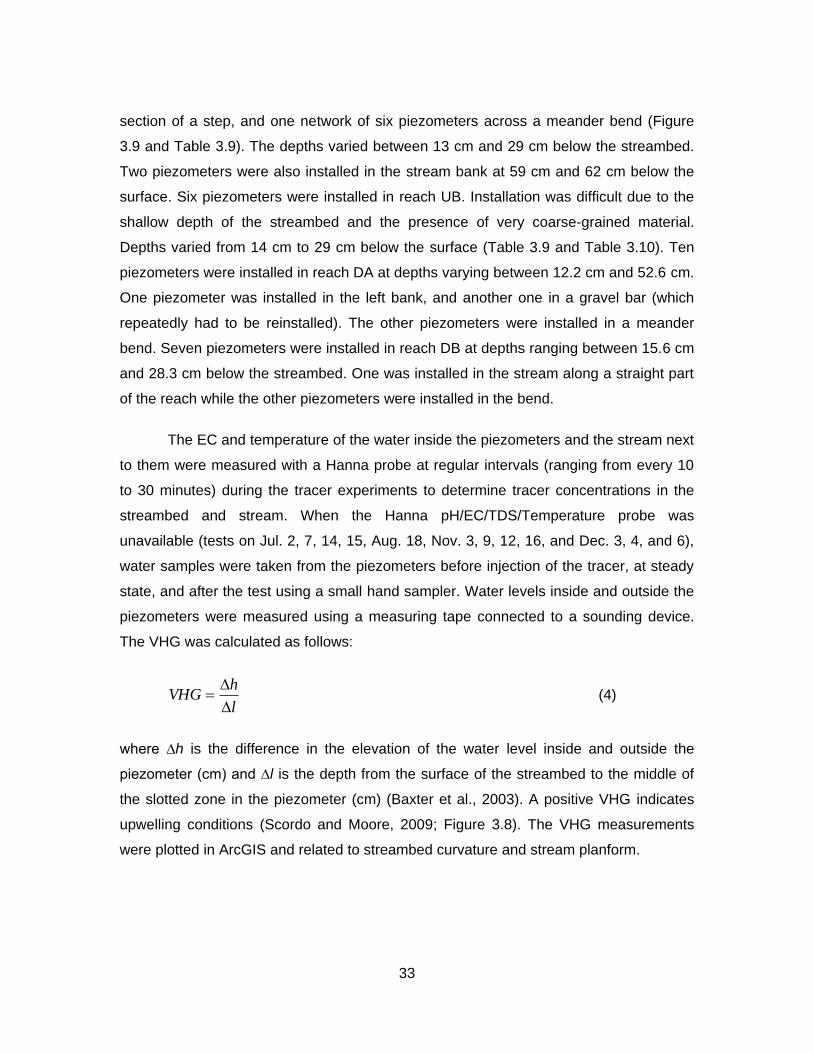
33

section of a step, and one network of six piezometers across a meander bend (Figure

3.9 and Table 3.9). The depths varied between 13 cm and 29 cm below the streambed.

Two piezometers were also installed in the stream bank at 59 cm and 62 cm below the

surface. Six piezometers were installed in reach UB. Installation was difficult due to the

shallow depth of the streambed and the presence of very coarse-grained material.

Depths varied from 14 cm to 29 cm below the surface (Table 3.9 and Table 3.10). Ten

piezometers were installed in reach DA at depths varying between 12.2 cm and 52.6 cm.

One piezometer was installed in the left bank, and another one in a gravel bar (which

repeatedly had to be reinstalled). The other piezometers were installed in a meander

bend. Seven piezometers were installed in reach DB at depths ranging between 15.6 cm

and 28.3 cm below the streambed. One was installed in the stream along a straight part

of the reach while the other piezometers were installed in the bend.

The EC and temperature of the water inside the piezometers and the stream next

to them were measured with a Hanna probe at regular intervals (ranging from every 10

to 30 minutes) during the tracer experiments to determine tracer concentrations in the

streambed and stream. When the Hanna pH/EC/TDS/Temperature probe was

unavailable (tests on Jul. 2, 7, 14, 15, Aug. 18, Nov. 3, 9, 12, 16, and Dec. 3, 4, and 6),

water samples were taken from the piezometers before injection of the tracer, at steady

state, and after the test using a small hand sampler. Water levels inside and outside the

piezometers were measured using a measuring tape connected to a sounding device.

The VHG was calculated as follows:

l

hVHG

(4)

where ∆h is the difference in the elevation of the water level inside and outside the

piezometer (cm) and ∆l is the depth from the surface of the streambed to the middle of

the slotted zone in the piezometer (cm) (Baxter et al., 2003). A positive VHG indicates

upwelling conditions (Scordo and Moore, 2009; Figure 3.8). The VHG measurements

were plotted in ArcGIS and related to streambed curvature and stream planform.

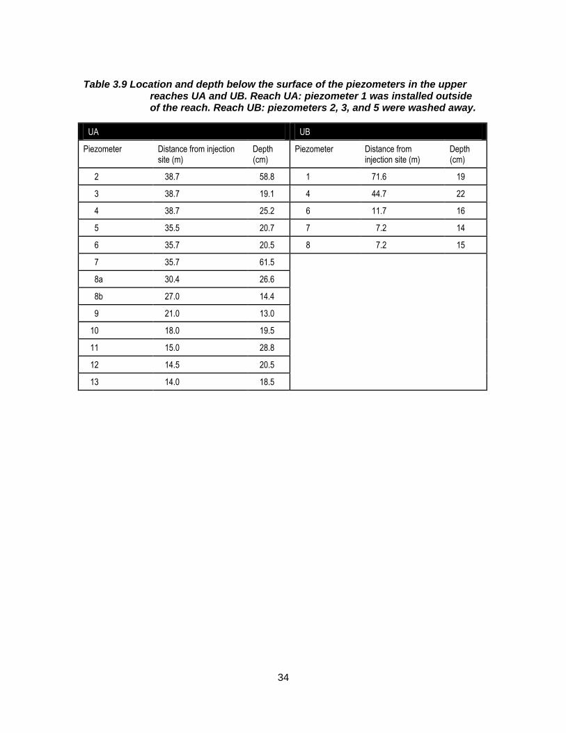
34

Table 3.9 Location and depth below the surface of the piezometers in the upper reaches UA and UB. Reach UA: piezometer 1 was installed outside of the reach. Reach UB: piezometers 2, 3, and 5 were washed away.

UA UB

Piezometer Distance from injection site (m)

Depth (cm)

Piezometer Distance from injection site (m)

Depth (cm)

2 38.7 58.8 1 71.6 19

3 38.7 19.1 4 44.7 22

4 38.7 25.2 6 11.7 16

5 35.5 20.7 7 7.2 14

6 35.7 20.5 8 7.2 15

7 35.7 61.5

8a 30.4 26.6

8b 27.0 14.4

9 21.0 13.0

10 18.0 19.5

11 15.0 28.8

12 14.5 20.5

13 14.0 18.5

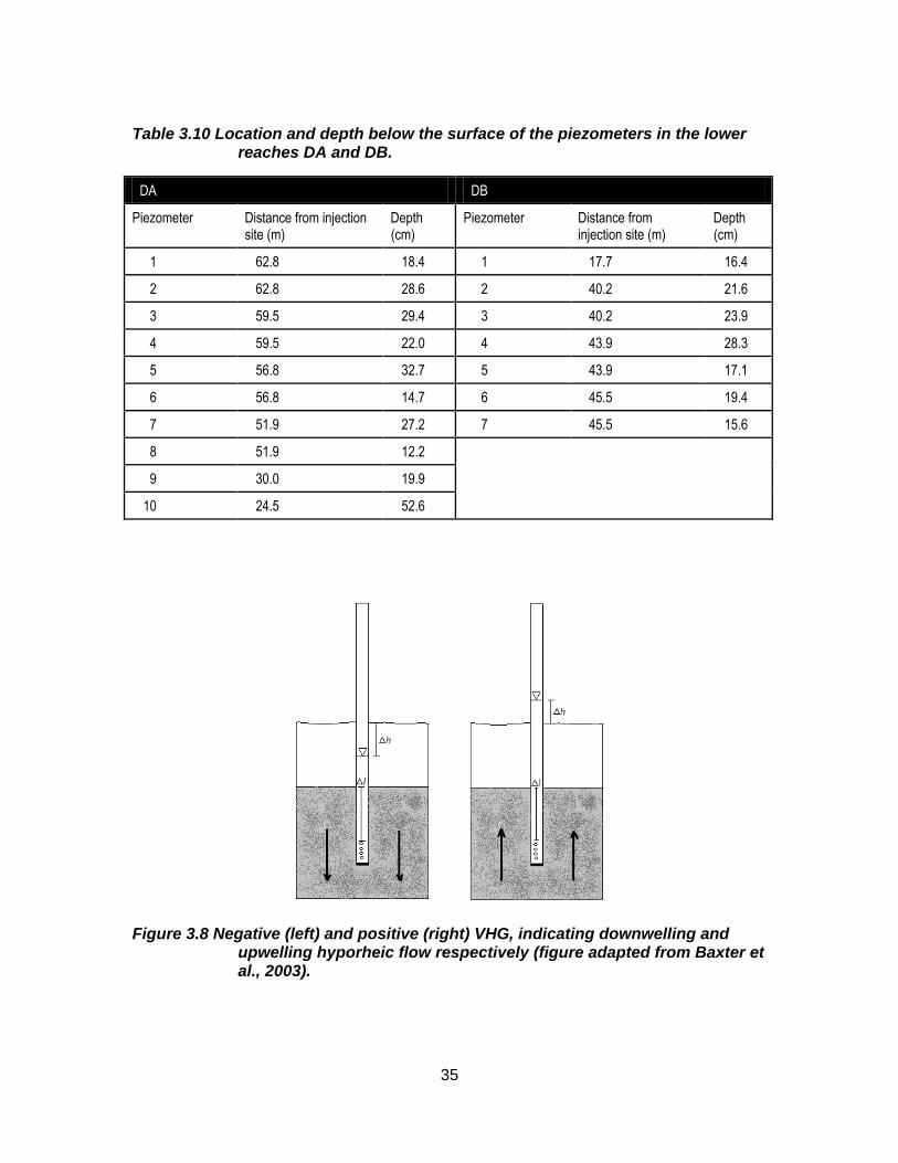
35

Table 3.10 Location and depth below the surface of the piezometers in the lower reaches DA and DB.

DA DB

Piezometer Distance from injection site (m)

Depth (cm)

Piezometer Distance from injection site (m)

Depth (cm)

1 62.8 18.4 1 17.7 16.4

2 62.8 28.6 2 40.2 21.6

3 59.5 29.4 3 40.2 23.9

4 59.5 22.0 4 43.9 28.3

5 56.8 32.7 5 43.9 17.1

6 56.8 14.7 6 45.5 19.4

7 51.9 27.2 7 45.5 15.6

8 51.9 12.2

9 30.0 19.9

10 24.5 52.6

Figure 3.8 Negative (left) and positive (right) VHG, indicating downwelling and upwelling hyporheic flow respectively (figure adapted from Baxter et al., 2003).

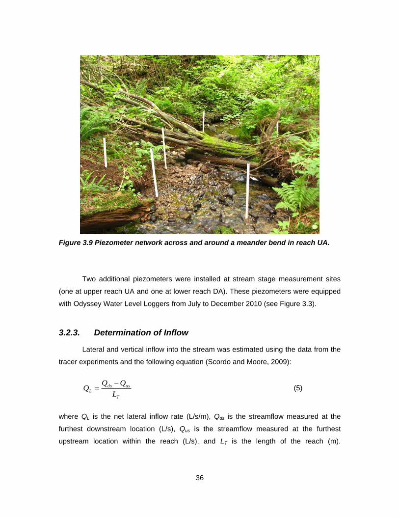
36

Figure 3.9 Piezometer network across and around a meander bend in reach UA.

Two additional piezometers were installed at stream stage measurement sites

(one at upper reach UA and one at lower reach DA). These piezometers were equipped

with Odyssey Water Level Loggers from July to December 2010 (see Figure 3.3).

3.2.3. Determination of Inflow

Lateral and vertical inflow into the stream was estimated using the data from the

tracer experiments and the following equation (Scordo and Moore, 2009):

T

usds

LL

QQQ

(5)

where QL is the net lateral inflow rate (L/s/m), Qds is the streamflow measured at the

furthest downstream location (L/s), Qus is the streamflow measured at the furthest

upstream location within the reach (L/s), and LT is the length of the reach (m).

37

Streamflow was calculated for each measurement location using the following equation

(Moore, 2004):

bgss ECECk

qQ

(6)

where Q is discharge (L/s), q is the injection rate (L/s), k is the slope of the relation

between the relative concentration at steady state and EC (where the relative

concentration is equal to the injection rate divided by the sum of the injection rate and

stream discharge), and ECbg and ECss are the electrical conductivities of stream water at

background (before injection of tracer) and steady state (during the tracer injection)

respectively.

3.2.4. Topographic Surveys

The reaches were surveyed using a Topcon total station. For reach UA 1247

points were surveyed, for reach UB 1105 data points, for DA 1042 points, and reach DB

830 data points. These data points were mapped in ArcGIS to create various maps

showing probe and piezometer locations, as well as DEMs of each reach. These

topographic surveys were used to determine the gradient of each reach in order to

determine whether or not topography could predict the location of lateral inflows in each

reach. All culverts and other drainage features were mapped as well (Figure 3.3).

3.2.5. Modeling with OTIS and OTIS-P

3.2.5.1. Calibration

OTIS and OTIS-P (see section 2.4) were used to model the movement of the

tracer through the stream and streambed, and to determine transient storage in the

stream and the rate of hyporheic exchange. OTIS-P solves equations 1 and 2 to

estimate advection, dispersion, lateral inflow, and transient storage. The parameters that

were optimized using OTIS-P are: the cross-sectional area of the stream (A), the cross-

sectional area of the storage zone (As), the dispersion (D), and storage zone exchange

coefficient (α). OTIS-P adjusts these values to create a curve that best fits the observed

38

breakthrough data at the YSI and ECH2O probe locations (Table 3.6 and Table 3.7)

during the tracer experiments. The Spearman rank correlation coefficient (rs) was

determined for the relation between the optimized parameters and discharge.

Other parameters can be estimated based on the values of the parameters that

were optimized in OTIS-P. These include the standardized storage zone to stream

cross-sectional area (As/A) that allows for comparisons between streams and reaches,

and the storage zone residence time (TSZ), which is the average time a molecule is

stored in transient storage (Thackston and Schnelle, 1970):

A

AT s

SZ (7)

The hydraulic retention factor (Rh), a measure of the average time a water molecule is

stored relative to the hydraulic turnover length, can be calculated using the following

equation (Morrice et al., 1997):

Q

AR s

h , (8)

where Q is the discharge (m3/s). Finally, the average distance a water molecule travels

in the stream before entering transient storage (Ls) can be calculated using the equation

(Fabian et al., 2011):

A

QLs (9)

Parameter uncertainty is an inevitable part of any transient storage model. By

analyzing the Damköhler number (DaI), stream velocity and reach length, an appropriate

reach length can be chosen. The DaI is a dimensionless combination of the rates of

exchange between stream and storage zones and is computed using the following

equation:

u

LA

A

DaIs

1

, (10)

39

where L is the length of the reach (m), u is the average water velocity (m/s), α is the

stream-storage exchange coefficient (s-1), and As is the storage zone cross-sectional

area (m2) (Wagner and Harvey, 1997). Uncertainty in the optimized hyporheic exchange

parameters is lowest when DaI=1, and increases as DaI values deviate from 1. DaI less

than ‘1’ have a higher uncertainty because only small amounts of tracer interact with the

storage zones in the reach and indicate that reach length may be too long or the velocity

is too high. DaI greater than ‘1’ have a higher uncertainty because all solute interacts

with the storage zones in the reach and indicate that the reach lengths may be too short

or the velocity is too low.

Input files for OTIS-P include the control file (used to specify the file names of the

input and output files), parameter file (which has information on the time, reach/sub-

reach length data, and As, D, and α estimates), flow file (which contains discharge data

and estimates for the A parameter), data file (which contains concentration data from the

YSI and ECH2O probes), and the STARPAC input file (which is used to indicate which

parameters are optimized and which parameters are held constant). There were too

many concentration data points for the data input file. Therefore not all data points were

included in the data file and only those data points just before the injection of the solute

started until steady state was reached were included. Initial values for the A, As, D, and α

parameters were based on previous OTIS-P runs; the OTIS-P runs were carried out in

order from the experiment with the lowest to highest discharge. At the start of each

calibration run, the same parameter values were assigned for all segments of the reach.

Once OTIS-P was run, the optimized parameter values were inserted into the parameter

input files and OTIS-P was run again. This process was repeated until OTIS-P yielded

stable optimized parameter values.

3.2.5.2. Validation

Using the calibrated parameter values from OTIS-P, OTIS was used for

validation of the model. OTIS requires fewer input files than OTIS-P, which include the

control file (used to specify the filenames of the remaining input and output files),

parameter file (contains the time, reach/sub-reach length data and the parameter values

for As, D, and α), and flow file (contains the discharge data and the optimized value of

A). All additional data (DEC probes and stream and streambed data from the piezometer

40

sites) were used for validation of the model. Goodness of fit statistics included the

correlation coefficient (R), Nash-Sutcliffe Efficiency (E), and Mean Squared Error (MSE).

41

4. Results and Discussion

4.1. Streamflow

Forty tracer tests were conducted: 10 at each reach. However, because of rain

events, unforeseen flooding, and equipment malfunction, not all tests could be used for

analysis (September 28 and July 7, 2010 (UA), August 4, 2010 (DB), October 27, 2010

(UB), and November 9, 2010 (DA)). Discharge during the tracer tests varied between 1

and 72 L/s for the upstream reaches and between 19 and 335 L/s for the downstream

reaches (Table 4.1 and Table 4.2). Previous tracer studies have been conducted for

discharge varying from <1-250 L/s (Webster and Valett, 2007). Not many studies that

examined hyporheic exchange have been conducted under high flow conditions that are

comparable to the high flows in the downstream reaches during this study. The highest

discharge in tracer studies relating specifically to hyporheic exchange ranged between

30-75 L/s (Morrice et al., 1997; Hart et al., 1999; Patschke, 1999; Scordo and Moore,

2009; Ryan et al., 2010).

The urban setting was initially thought to be “more controlled” than a natural

forest setting, but in fact was less controlled. Unknown drainage networks and crossings

led to more unknowns than in a relatively untouched forest setting. For example, there

were regular rapid increases in discharge during the summer despite a lack of

precipitation (Figure 4.1). Streamflow increased by 1.1-29 L/s during twenty of these

events between July 10 and August 31, 2010. The volume added to the stream ranged

from 14 to 457 m3. Inquiries were made to the City of Coquitlam concerning these flow

increases; however, their responses regarding the source of this water do not seem

plausible (e.g. it was suggested that this was due to the spray park, which is located

downstream of the study reaches; diversion of water from the park would not contribute

to the stream reaches at a higher elevation). Other examples of potential sources of flow

changes included obstructions placed into the stream, such as rocks, to create small

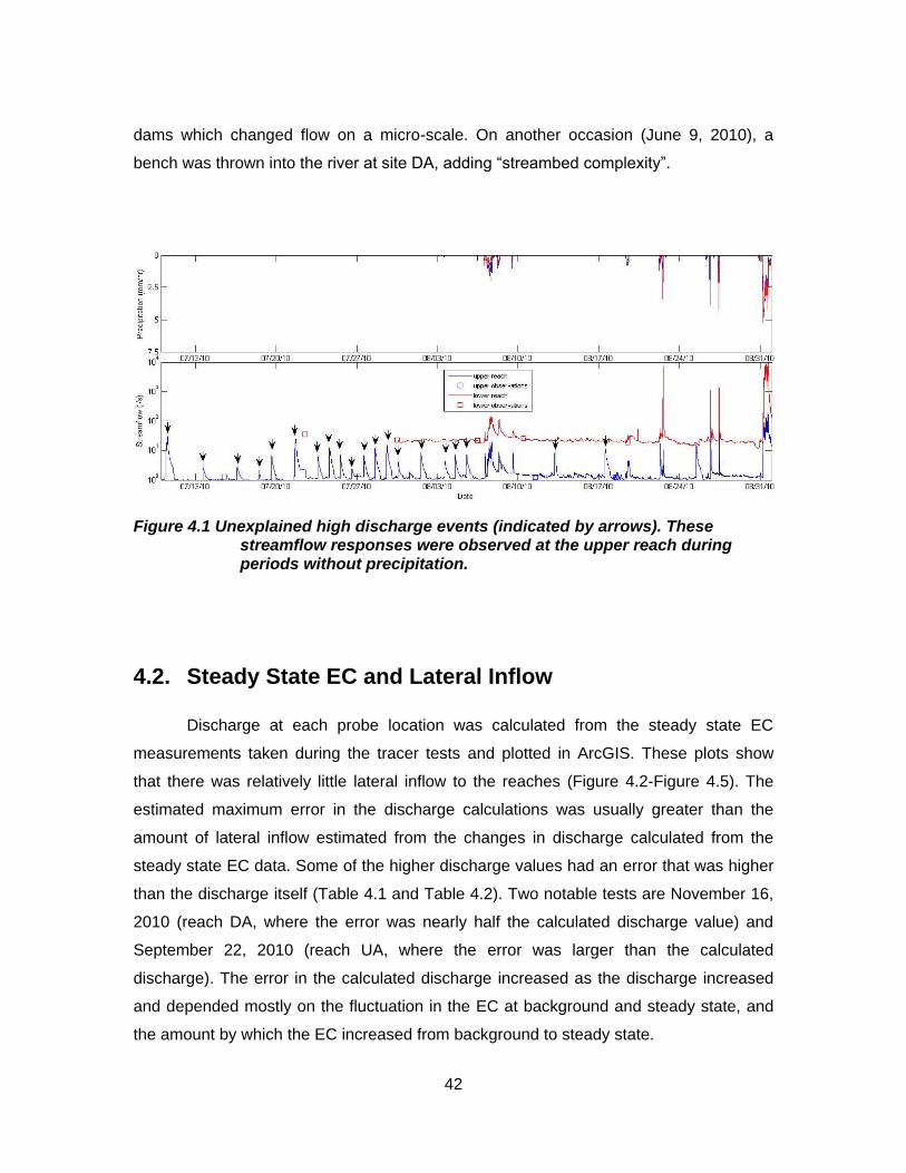
42

dams which changed flow on a micro-scale. On another occasion (June 9, 2010), a

bench was thrown into the river at site DA, adding “streambed complexity”.

Figure 4.1 Unexplained high discharge events (indicated by arrows). These streamflow responses were observed at the upper reach during periods without precipitation.

4.2. Steady State EC and Lateral Inflow

Discharge at each probe location was calculated from the steady state EC

measurements taken during the tracer tests and plotted in ArcGIS. These plots show

that there was relatively little lateral inflow to the reaches (Figure 4.2-Figure 4.5). The

estimated maximum error in the discharge calculations was usually greater than the

amount of lateral inflow estimated from the changes in discharge calculated from the

steady state EC data. Some of the higher discharge values had an error that was higher

than the discharge itself (Table 4.1 and Table 4.2). Two notable tests are November 16,

2010 (reach DA, where the error was nearly half the calculated discharge value) and

September 22, 2010 (reach UA, where the error was larger than the calculated

discharge). The error in the calculated discharge increased as the discharge increased

and depended mostly on the fluctuation in the EC at background and steady state, and

the amount by which the EC increased from background to steady state.

43

The maps of steady state discharge (Figure 4.2-Figure 4.5) and steady state EC

measured with the handheld probe (or YSI, ECH2O, and DEC probes when the handheld

probe was unavailable; Appendix B) reveal no clear pattern as to whether discharge

increased along the reaches or not and instead show high variability in discharge on the

different days. The average rank of the steady state EC values and standard deviation

(SD) of the rank were calculated to determine the temporal stability (i.e. temporal

persistence) of the variation in discharge along the reach (Figure 4.6 and Figure 4.7).

This was done by assigning a rank to the steady state EC value at each probe location

for each test, and then determining the average and standard deviation (SD) of the rank

for each specific probe location (see Appendix A for the calculation). A high average

rank indicates a persistently low steady state EC (and therefore high discharge), while a

low average rank indicates a persistently high steady state EC (and therefore low

discharge). An intermediate average rank, with a high standard deviation in rank

indicates a highly variable rank, and thus no persistent pattern in the steady state EC

values.

For reach UA, steady state EC was relatively similar throughout the reach. The

average rank varied between 4.0 and 5.9 (SD ranged from 1.9-3.8), indicating little

persistent variation in steady state EC throughout the reach. In the step-pool near the

beginning of the reach and through the bend downstream, discharge was generally

lowest, with an average rank between 4.1 and 4.3.

The average rank for reach UB varied between 2.1 and 5.6 (SD ranged from 1.3-

2.3), indicating more persistent variation in steady state EC between sites within the

reach. Sites just before the bifurcation in the middle of reach UB had the lowest average

rank (2.05, SD of 1.3) (and thus the lowest discharge); the site just after the

convergence of the stream had the highest average rank (5.6, SD of 2.1) (thus highest

discharge). Where the reach was narrower, the average rank varied between 2.1 and

4.2.

Average rank for reach DA varied between 1.6 and 5.2 (SD ranged from 2.1-2.7),

indicating some persistent differences in steady state EC between sites. The average

rank of steady state EC decreased somewhat towards the end of the reach, indicating

decreasing streamflow in the slow moving part of the stream after a meander bend.

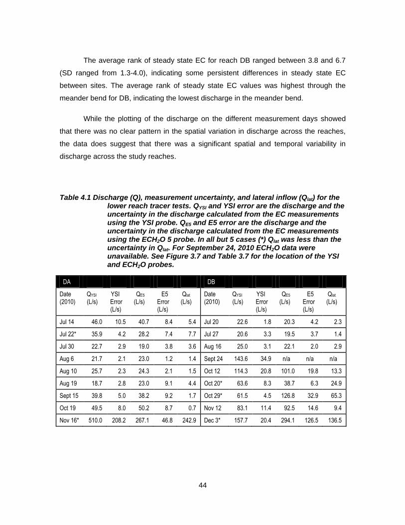
44

The average rank of steady state EC for reach DB ranged between 3.8 and 6.7

(SD ranged from 1.3-4.0), indicating some persistent differences in steady state EC

between sites. The average rank of steady state EC values was highest through the

meander bend for DB, indicating the lowest discharge in the meander bend.

While the plotting of the discharge on the different measurement days showed

that there was no clear pattern in the spatial variation in discharge across the reaches,

the data does suggest that there was a significant spatial and temporal variability in

discharge across the study reaches.

Table 4.1 Discharge (Q), measurement uncertainty, and lateral inflow (Qlat) for the lower reach tracer tests. QYSI and YSI error are the discharge and the uncertainty in the discharge calculated from the EC measurements using the YSI probe. QE5 and E5 error are the discharge and the uncertainty in the discharge calculated from the EC measurements using the ECH2O 5 probe. In all but 5 cases (*) Qlat was less than the uncertainty in Qlat. For September 24, 2010 ECH2O data were unavailable. See Figure 3.7 and Table 3.7 for the location of the YSI and ECH2O probes.

DA DB

Date (2010)

QYSI (L/s)

YSI Error (L/s)

QE5 (L/s)

E5 Error (L/s)

Qlat (L/s)

Date (2010)

QYSI (L/s)

YSI Error (L/s)

QE5 (L/s)

E5 Error (L/s)

Qlat (L/s)

Jul 14 46.0 10.5 40.7 8.4 5.4 Jul 20 22.6 1.8 20.3 4.2 2.3

Jul 22* 35.9 4.2 28.2 7.4 7.7 Jul 27 20.6 3.3 19.5 3.7 1.4

Jul 30 22.7 2.9 19.0 3.8 3.6 Aug 16 25.0 3.1 22.1 2.0 2.9

Aug 6 21.7 2.1 23.0 1.2 1.4 Sept 24 143.6 34.9 n/a n/a n/a

Aug 10 25.7 2.3 24.3 2.1 1.5 Oct 12 114.3 20.8 101.0 19.8 13.3

Aug 19 18.7 2.8 23.0 9.1 4.4 Oct 20* 63.6 8.3 38.7 6.3 24.9

Sept 15 39.8 5.0 38.2 9.2 1.7 Oct 29* 61.5 4.5 126.8 32.9 65.3

Oct 19 49.5 8.0 50.2 8.7 0.7 Nov 12 83.1 11.4 92.5 14.6 9.4

Nov 16* 510.0 208.2 267.1 46.8 242.9 Dec 3* 157.7 20.4 294.1 126.5 136.5

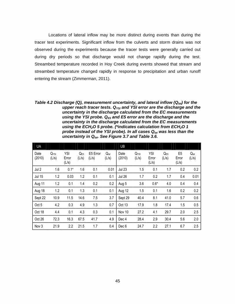
45

Locations of lateral inflow may be more distinct during events than during the

tracer test experiments. Significant inflow from the culverts and storm drains was not

observed during the experiments because the tracer tests were generally carried out

during dry periods so that discharge would not change rapidly during the test.

Streambed temperature recorded in Hoy Creek during events showed that stream and

streambed temperature changed rapidly in response to precipitation and urban runoff

entering the stream (Zimmerman, 2011).

Table 4.2 Discharge (Q), measurement uncertainty, and lateral inflow (Qlat) for the upper reach tracer tests. QYSI and YSI error are the discharge and the uncertainty in the discharge calculated from the EC measurements using the YSI probe. QE5 and E5 error are the discharge and the uncertainty in the discharge calculated from the EC measurements using the ECH2O 5 probe. (*indicates calculation from ECH2O 1 probe instead of the YSI probe). In all cases Qlat was less than the uncertainty in Qlat. See Figure 3.7 and Table 3.6.

UA UB

Date (2010)

QYSI (L/s)

YSI Error (L/s)

QE5 (L/s)

E5 Error (L/s)

Qlat (L/s)

Date (2010)

QYSI (L/s)

YSI Error (L/s)

QE5 (L/s)

E5 Error (L/s)

Qlat (L/s)

Jul 2 1.6 0.1* 1.6 0.1 0.01 Jul 23 1.5 0.1 1.7 0.2 0.2

Jul 15 1.2 0.03 1.2 0.1 0.1 Jul 26 1.7 0.2 1.7 0.4 0.01

Aug 11 1.2 0.1 1.4 0.2 0.2 Aug 5 3.6 0.6* 4.0 0.4 0.4

Aug 18 1.2 0.1 1.3 0.1 0.1 Aug 12 1.5 0.1 1.6 0.2 0.2

Sept 22 10.9 11.5 14.6 7.5 3.7 Sept 29 40.4 8.1 41.0 5.7 0.6

Oct 5 4.2 0.3 4.9 1.3 0.7 Oct 13 17.9 1.8 17.4 1.5 0.5

Oct 18 4.4 0.1 4.3 0.3 0.1 Nov 10 27.2 4.1 29.7 2.0 2.5

Oct 26 72.3 16.3 67.5 41.7 4.9 Dec 4 28.4 2.9 30.4 5.6 2.0

Nov 3 21.9 2.2 21.5 1.7 0.4 Dec 6 24.7 2.2 27.1 6.7 2.5

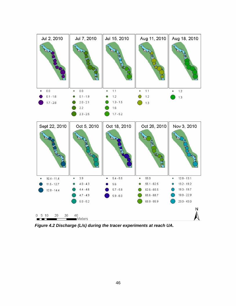
46

Figure 4.2 Discharge (L/s) during the tracer experiments at reach UA.

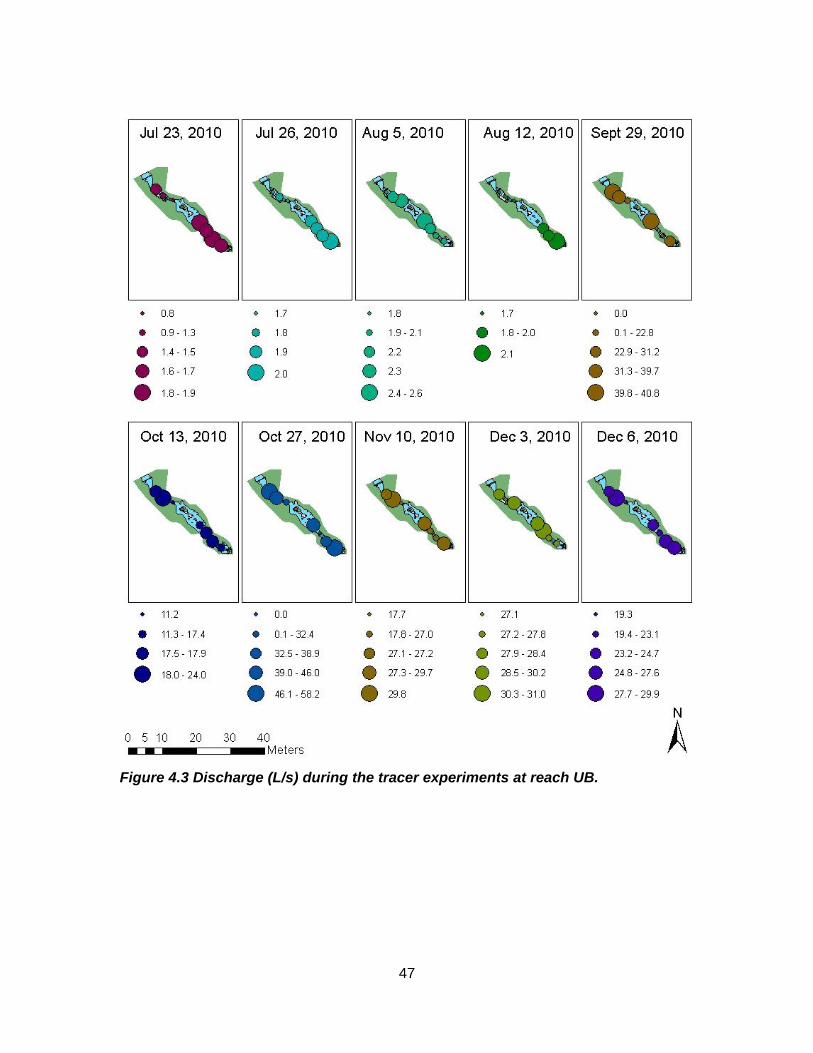
47

Figure 4.3 Discharge (L/s) during the tracer experiments at reach UB.

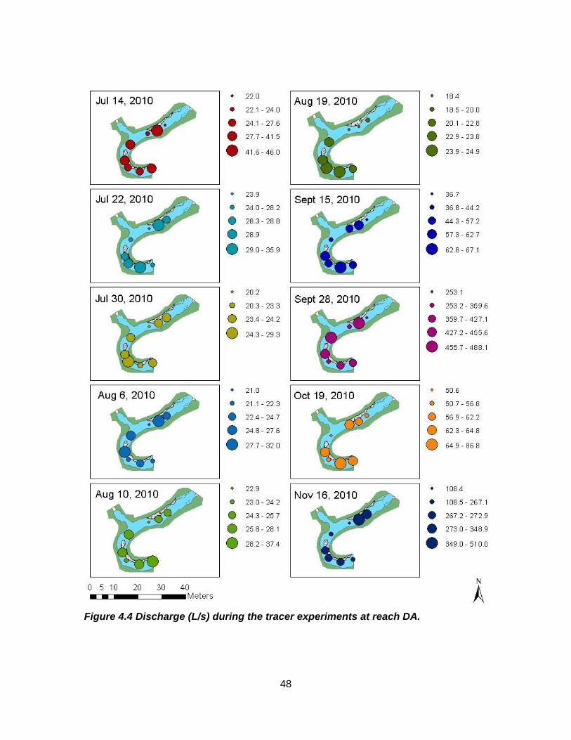
48

Figure 4.4 Discharge (L/s) during the tracer experiments at reach DA.

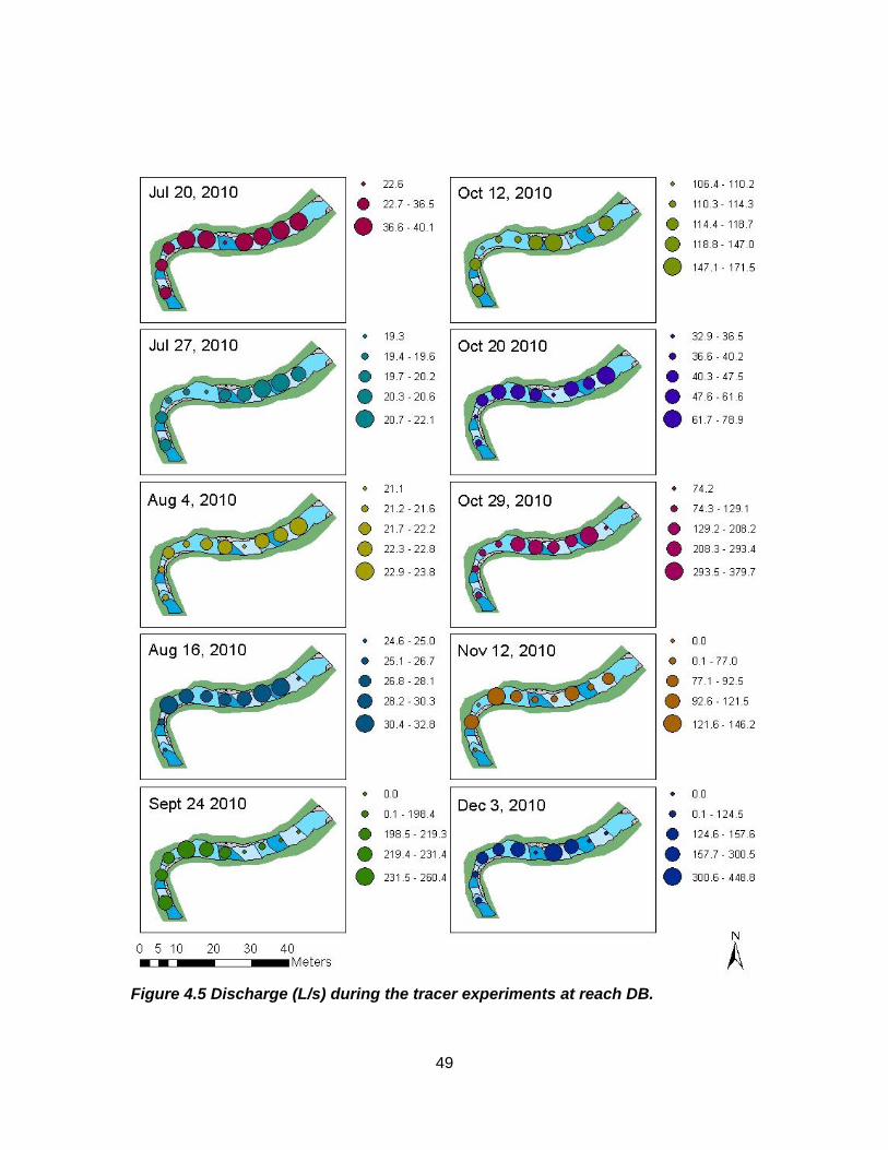
49

Figure 4.5 Discharge (L/s) during the tracer experiments at reach DB.

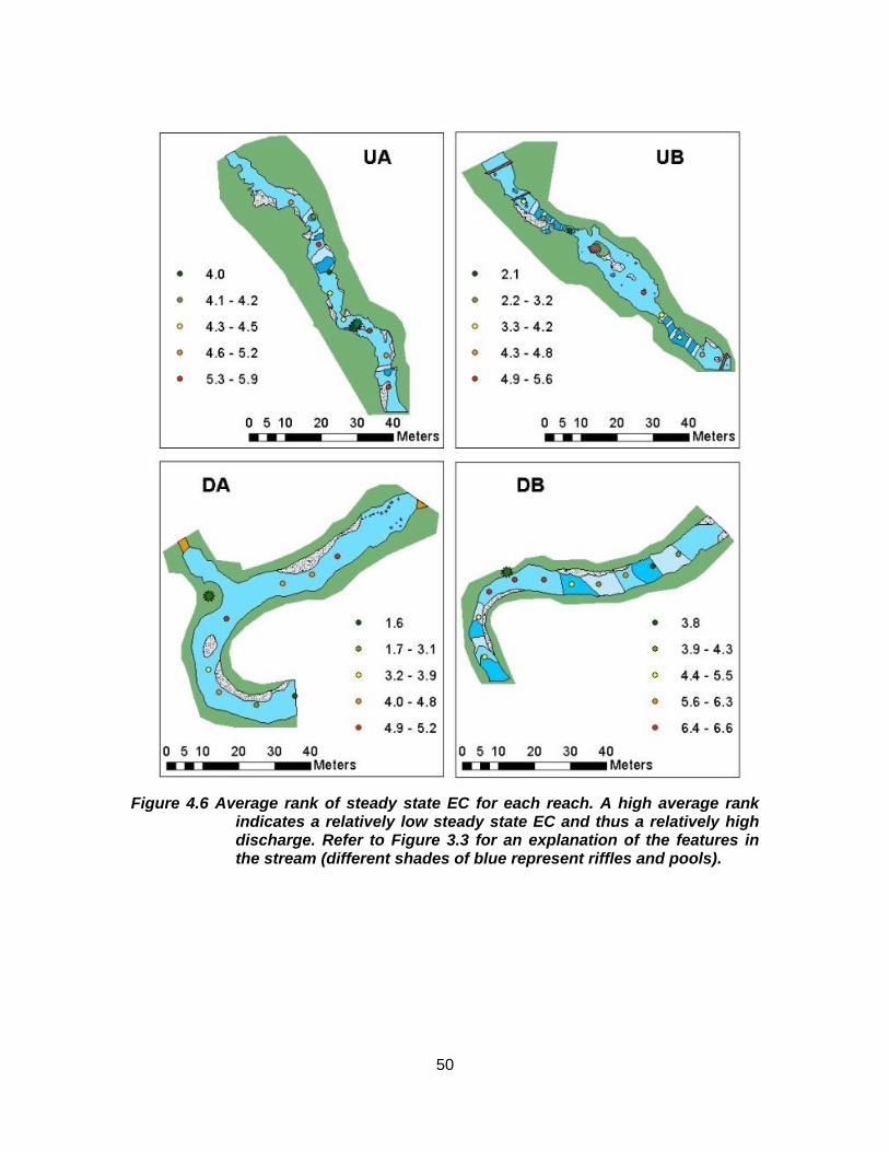
50

Figure 4.6 Average rank of steady state EC for each reach. A high average rank indicates a relatively low steady state EC and thus a relatively high discharge. Refer to Figure 3.3 for an explanation of the features in the stream (different shades of blue represent riffles and pools).

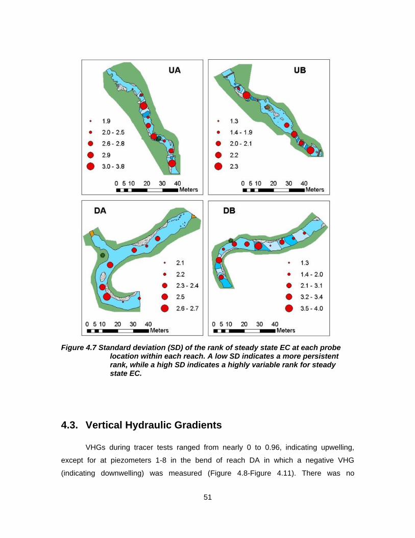
51

Figure 4.7 Standard deviation (SD) of the rank of steady state EC at each probe location within each reach. A low SD indicates a more persistent rank, while a high SD indicates a highly variable rank for steady state EC.

4.3. Vertical Hydraulic Gradients

VHGs during tracer tests ranged from nearly 0 to 0.96, indicating upwelling,

except for at piezometers 1-8 in the bend of reach DA in which a negative VHG

(indicating downwelling) was measured (Figure 4.8-Figure 4.11). There was no

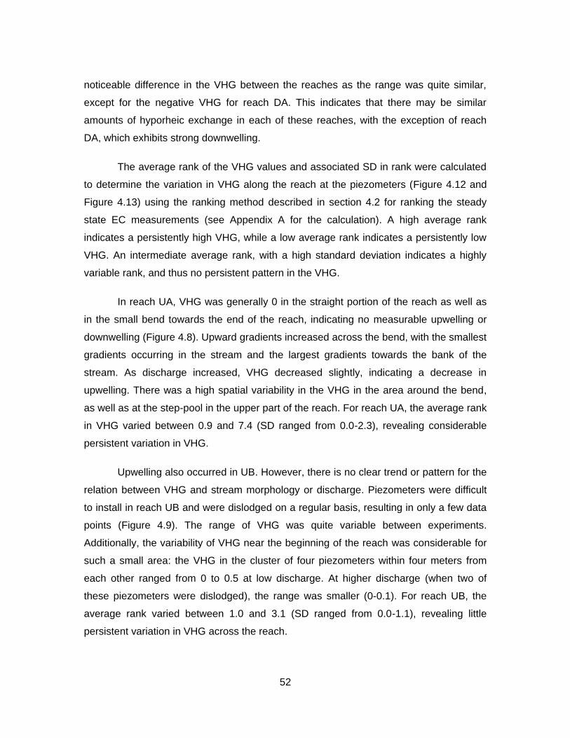
52

noticeable difference in the VHG between the reaches as the range was quite similar,

except for the negative VHG for reach DA. This indicates that there may be similar

amounts of hyporheic exchange in each of these reaches, with the exception of reach

DA, which exhibits strong downwelling.

The average rank of the VHG values and associated SD in rank were calculated

to determine the variation in VHG along the reach at the piezometers (Figure 4.12 and

Figure 4.13) using the ranking method described in section 4.2 for ranking the steady

state EC measurements (see Appendix A for the calculation). A high average rank

indicates a persistently high VHG, while a low average rank indicates a persistently low

VHG. An intermediate average rank, with a high standard deviation indicates a highly

variable rank, and thus no persistent pattern in the VHG.

In reach UA, VHG was generally 0 in the straight portion of the reach as well as

in the small bend towards the end of the reach, indicating no measurable upwelling or

downwelling (Figure 4.8). Upward gradients increased across the bend, with the smallest

gradients occurring in the stream and the largest gradients towards the bank of the

stream. As discharge increased, VHG decreased slightly, indicating a decrease in

upwelling. There was a high spatial variability in the VHG in the area around the bend,

as well as at the step-pool in the upper part of the reach. For reach UA, the average rank

in VHG varied between 0.9 and 7.4 (SD ranged from 0.0-2.3), revealing considerable

persistent variation in VHG.

Upwelling also occurred in UB. However, there is no clear trend or pattern for the

relation between VHG and stream morphology or discharge. Piezometers were difficult

to install in reach UB and were dislodged on a regular basis, resulting in only a few data

points (Figure 4.9). The range of VHG was quite variable between experiments.

Additionally, the variability of VHG near the beginning of the reach was considerable for

such a small area: the VHG in the cluster of four piezometers within four meters from

each other ranged from 0 to 0.5 at low discharge. At higher discharge (when two of

these piezometers were dislodged), the range was smaller (0-0.1). For reach UB, the

average rank varied between 1.0 and 3.1 (SD ranged from 0.0-1.1), revealing little

persistent variation in VHG across the reach.

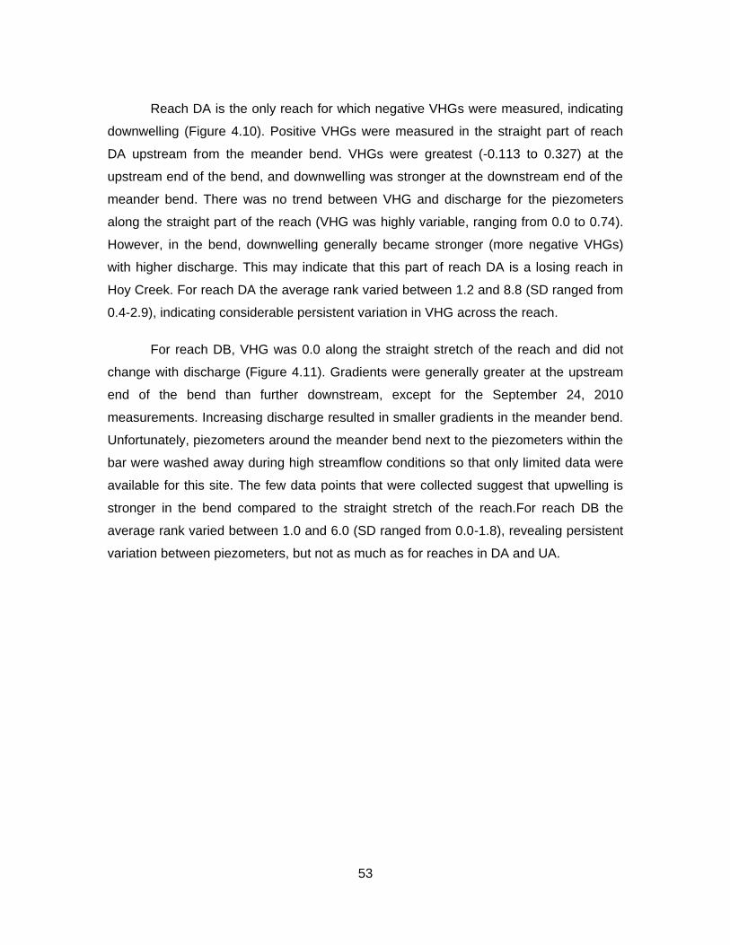
53

Reach DA is the only reach for which negative VHGs were measured, indicating

downwelling (Figure 4.10). Positive VHGs were measured in the straight part of reach

DA upstream from the meander bend. VHGs were greatest (-0.113 to 0.327) at the

upstream end of the bend, and downwelling was stronger at the downstream end of the

meander bend. There was no trend between VHG and discharge for the piezometers

along the straight part of the reach (VHG was highly variable, ranging from 0.0 to 0.74).

However, in the bend, downwelling generally became stronger (more negative VHGs)

with higher discharge. This may indicate that this part of reach DA is a losing reach in

Hoy Creek. For reach DA the average rank varied between 1.2 and 8.8 (SD ranged from

0.4-2.9), indicating considerable persistent variation in VHG across the reach.

For reach DB, VHG was 0.0 along the straight stretch of the reach and did not

change with discharge (Figure 4.11). Gradients were generally greater at the upstream

end of the bend than further downstream, except for the September 24, 2010

measurements. Increasing discharge resulted in smaller gradients in the meander bend.

Unfortunately, piezometers around the meander bend next to the piezometers within the

bar were washed away during high streamflow conditions so that only limited data were

available for this site. The few data points that were collected suggest that upwelling is

stronger in the bend compared to the straight stretch of the reach.For reach DB the

average rank varied between 1.0 and 6.0 (SD ranged from 0.0-1.8), revealing persistent

variation between piezometers, but not as much as for reaches in DA and UA.

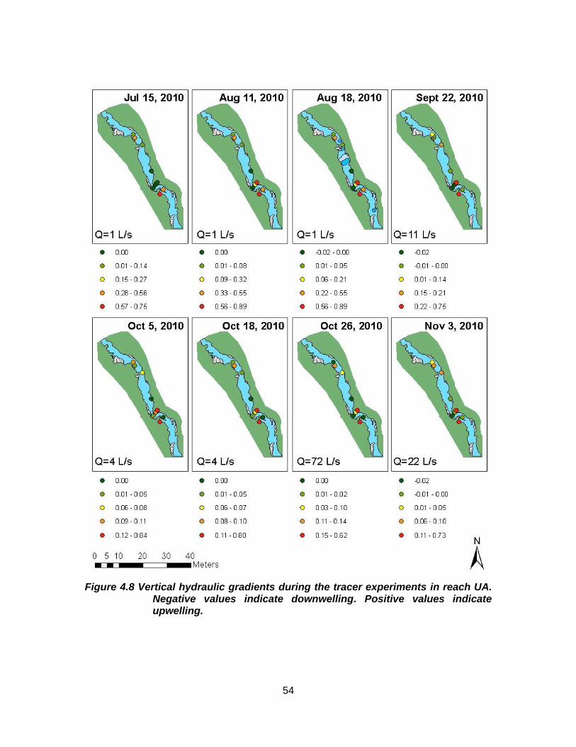
54

Figure 4.8 Vertical hydraulic gradients during the tracer experiments in reach UA. Negative values indicate downwelling. Positive values indicate upwelling.

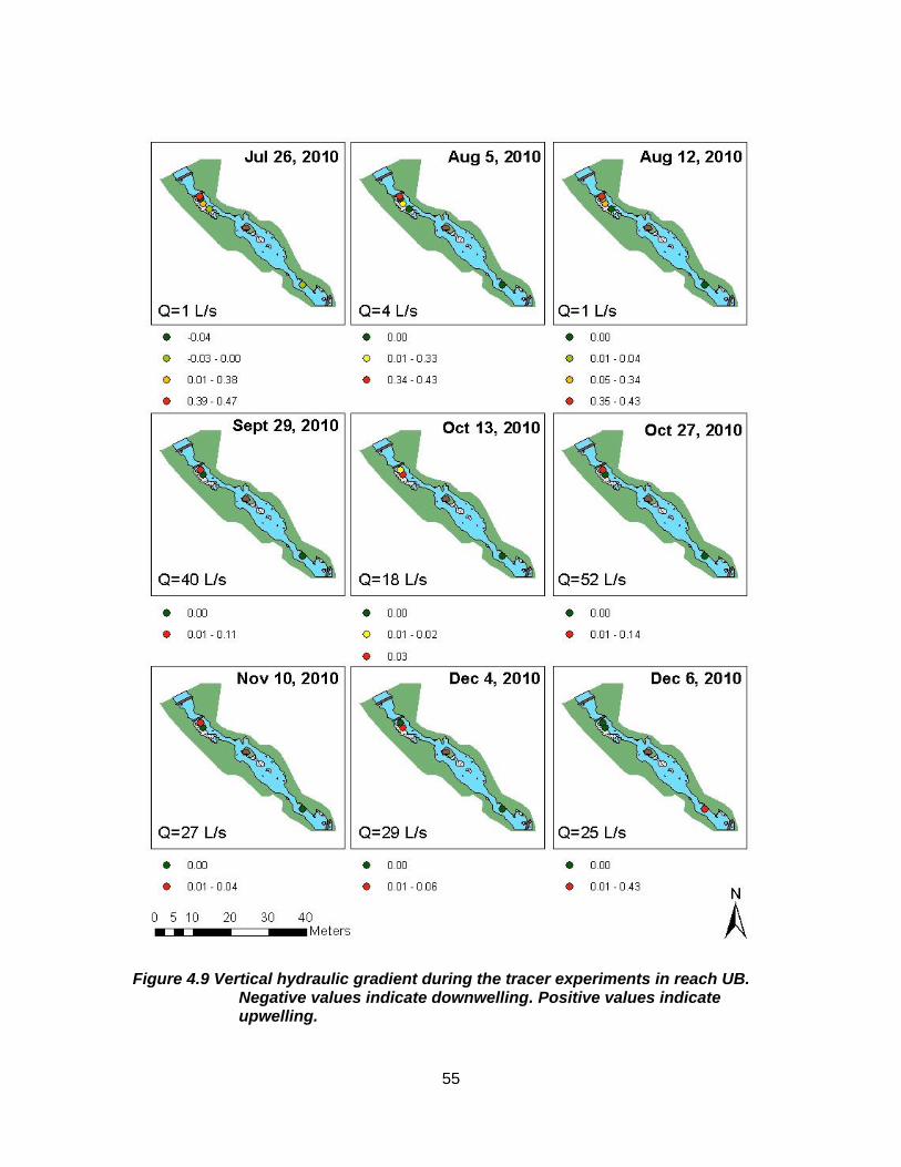
55

Figure 4.9 Vertical hydraulic gradient during the tracer experiments in reach UB. Negative values indicate downwelling. Positive values indicate upwelling.

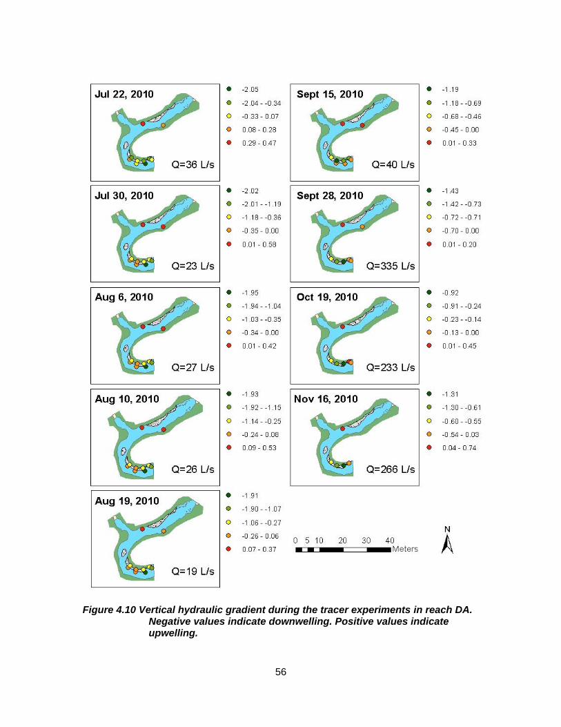
56

Figure 4.10 Vertical hydraulic gradient during the tracer experiments in reach DA. Negative values indicate downwelling. Positive values indicate upwelling.

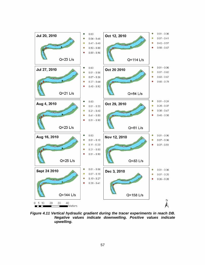
57

Figure 4.11 Vertical hydraulic gradient during the tracer experiments in reach DB. Negative values indicate downwelling. Positive values indicate upwelling.

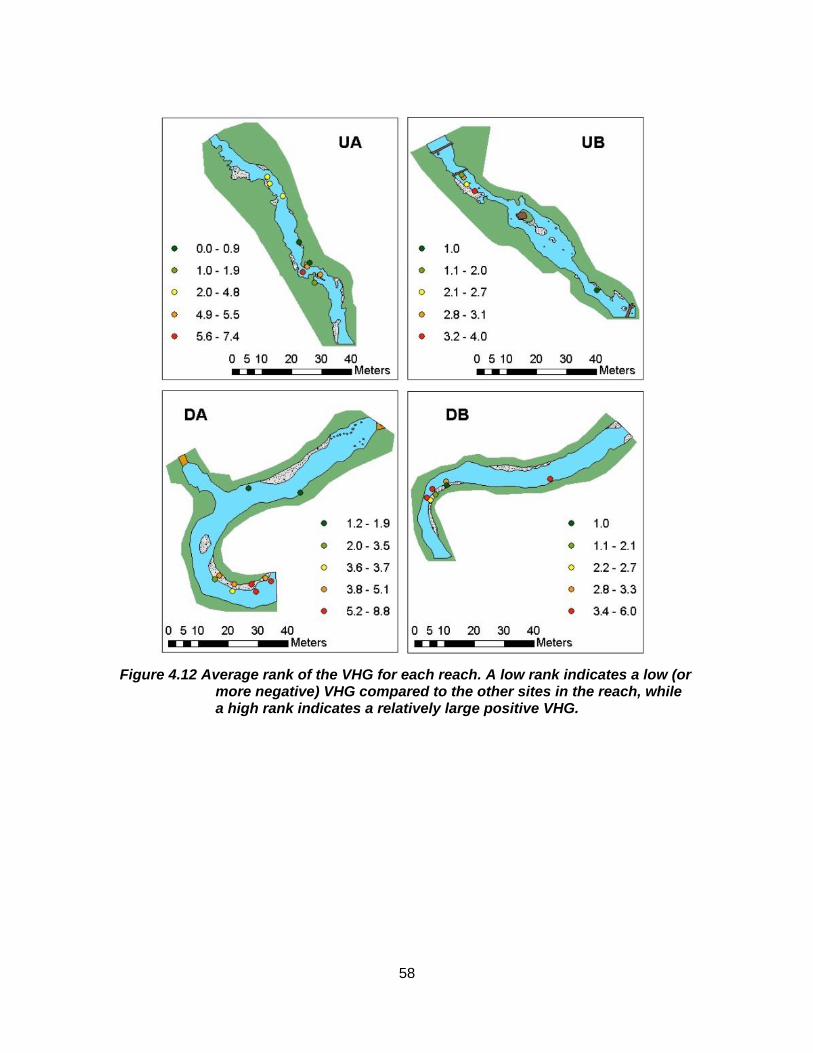
58

Figure 4.12 Average rank of the VHG for each reach. A low rank indicates a low (or more negative) VHG compared to the other sites in the reach, while a high rank indicates a relatively large positive VHG.

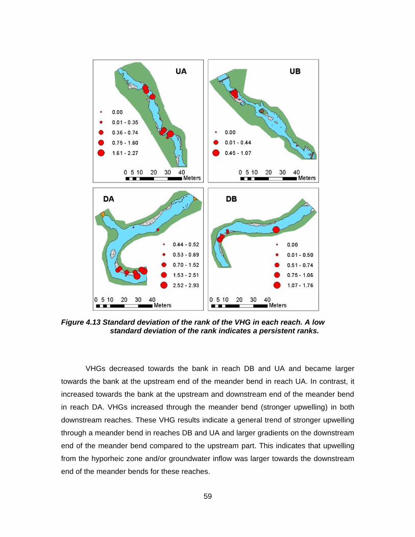
59

Figure 4.13 Standard deviation of the rank of the VHG in each reach. A low standard deviation of the rank indicates a persistent ranks.

VHGs decreased towards the bank in reach DB and UA and became larger

towards the bank at the upstream end of the meander bend in reach UA. In contrast, it

increased towards the bank at the upstream and downstream end of the meander bend

in reach DA. VHGs increased through the meander bend (stronger upwelling) in both

downstream reaches. These VHG results indicate a general trend of stronger upwelling

through a meander bend in reaches DB and UA and larger gradients on the downstream

end of the meander bend compared to the upstream part. This indicates that upwelling

from the hyporheic zone and/or groundwater inflow was larger towards the downstream

end of the meander bends for these reaches.

60

Upwelling occurred in the pool of the step near the upstream end of the reach.

The positive VHGs in the pool downstream of the step near the upstream end of reach

UA indicate inflow of hyporheic water and/or groundwater to the stream at that location.

Munz et al. (2011) showed that at the head of riffles and within pools, average VHG did

not exceed 0.025, indicating slight upwelling conditions. At the end of the riffle, VHG

increased to an average of 0.1, indicating increased upwelling. At the downstream end

of a pool, VHG decreased to 0.05-0.1, which is larger than upstream of the pool. For

reach UA, slight upwelling occurred in the pool near the beginning of the reach; this

observation was also supported by observations of tracer movement through the

piezometers located in the step and just downstream of the pool. These results support

the findings of Tonina and Buffington (2007) who noted that an obstruction creates high

pressure upstream, which drives hyporheic exchange. Munz et al. (2011) also observed

higher VHG variability as a result of sediment heterogeneity, which could explain the

high VHG variability at certain locations in the studied reaches in Hoy Creek (Figure 4.8-

Figure 4.11).

VHGs decreased as discharge increased in reaches UA and DB (weaker

upwelling). However, in reach DA, VHG decreased (stronger downwelling) as discharge

increased, similar to the results of Fabian et al. (2011), who showed that upwelling was

enhanced in upwelling zones at higher discharge. However, Fabian et al. (2011) also

noted weakened upwelling and downwelling zones during the transition from dry to wet

season due to a disruption of the equilibrium between groundwater and streamwater

levels, and different (ie. Deeper and longer) flow paths are used to reach different

upwelling and downwellng zones during different seasons, which is perhaps what occurs

in reaches UA and DB, where upwelling weakens with increasing discharge.

However, Fabian et al. (2011) also noted weaker upwelling and downwelling

during the transition from dry to wet season due to a disruption of the equilibrium

between groundwater and streamwater levels, and different (ie. deeper and longer) flow

paths to reach different upwelling and downwellng zones during different seasons.

Perhaps this occurred in reaches UA and DB, where upwelling weakened with

increasing discharge.

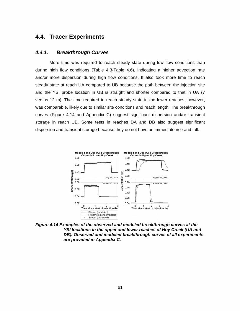
61

4.4. Tracer Experiments

4.4.1. Breakthrough Curves

More time was required to reach steady state during low flow conditions than

during high flow conditions (Table 4.3-Table 4.6), indicating a higher advection rate

and/or more dispersion during high flow conditions. It also took more time to reach

steady state at reach UA compared to UB because the path between the injection site

and the YSI probe location in UB is straight and shorter compared to that in UA (7

versus 12 m). The time required to reach steady state in the lower reaches, however,

was comparable, likely due to similar site conditions and reach length. The breakthrough

curves (Figure 4.14 and Appendix C) suggest significant dispersion and/or transient

storage in reach UB. Some tests in reaches DA and DB also suggest significant

dispersion and transient storage because they do not have an immediate rise and fall.

Figure 4.14 Examples of the observed and modeled breakthrough curves at the YSI locations in the upper and lower reaches of Hoy Creek (UA and DB). Observed and modeled breakthrough curves of all experiments are provided in Appendix C.

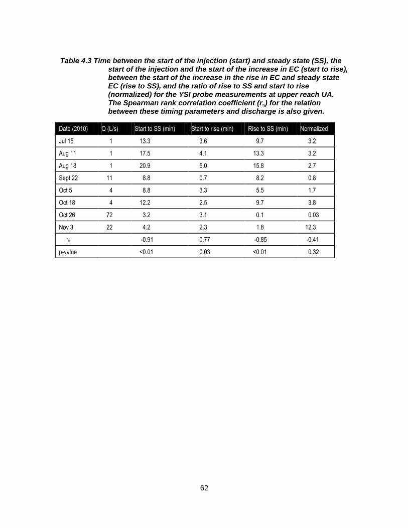
62

Table 4.3 Time between the start of the injection (start) and steady state (SS), the start of the injection and the start of the increase in EC (start to rise), between the start of the increase in the rise in EC and steady state EC (rise to SS), and the ratio of rise to SS and start to rise (normalized) for the YSI probe measurements at upper reach UA. The Spearman rank correlation coefficient (rs) for the relation between these timing parameters and discharge is also given.

Date (2010) Q (L/s) Start to SS (min) Start to rise (min) Rise to SS (min) Normalized

Jul 15 1 13.3 3.6 9.7 3.2

Aug 11 1 17.5 4.1 13.3 3.2

Aug 18 1 20.9 5.0 15.8 2.7

Sept 22 11 8.8 0.7 8.2 0.8

Oct 5 4 8.8 3.3 5.5 1.7

Oct 18 4 12.2 2.5 9.7 3.8

Oct 26 72 3.2 3.1 0.1 0.03

Nov 3 22 4.2 2.3 1.8 12.3

rs -0.91 -0.77 -0.85 -0.41

p-value <0.01 0.03 <0.01 0.32

63

Table 4.4 Time between the start of the injection (start) and steady state (SS), the start of the injection and the start of the increase in EC (start to rise), between the start of the increase in the rise in EC and steady state EC (rise to SS), and the ratio of rise to SS and start to rise (normalized) for the YSI probe measurements at upper reach UB. The Spearman rank correlation coefficient (rs) for the relation between these timing parameters and discharge is also given.

Date (2010) Q (L/s) Start to SS (min) Start to rise (min) Rise to SS (min) Normalized

Jul 23 1 6.3 1.5 4.8 3.2

Jul 26 1 5.3 1.7 3.7 2.2

Aug 12 1 6.0 1.5 4.5 3.0

Sept 29 40 2.0 1.0 1.0 1.0

Oct 13 18 3.8 0.5 3.3 7.7

Nov 10 27 4.3 3.0 1.3 0.4

Dec 4 29 2.7 0.3 2.3 7.0

Dec 6 25 2.8 0.6 2.3 4.2

rs -0.90 -0.39 -0.90 -0.05

p-value >0.01 0.34 >0.01 0.91

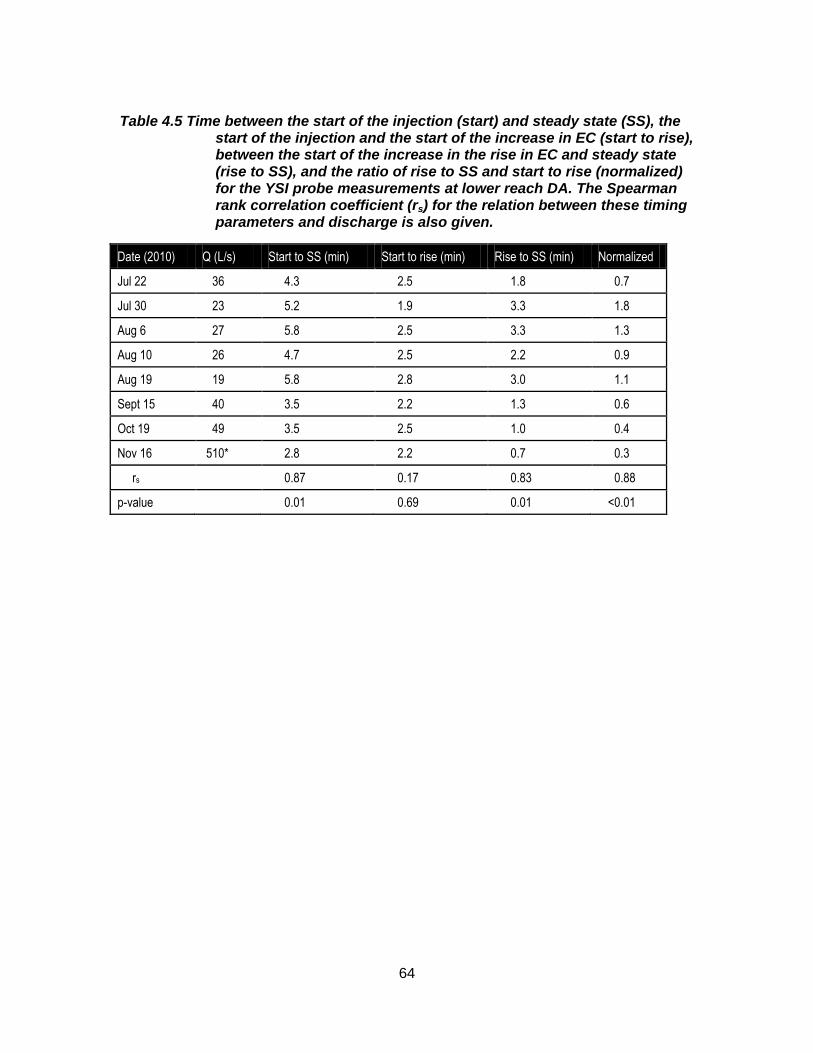
64

Table 4.5 Time between the start of the injection (start) and steady state (SS), the start of the injection and the start of the increase in EC (start to rise), between the start of the increase in the rise in EC and steady state (rise to SS), and the ratio of rise to SS and start to rise (normalized) for the YSI probe measurements at lower reach DA. The Spearman rank correlation coefficient (rs) for the relation between these timing parameters and discharge is also given.

Date (2010) Q (L/s) Start to SS (min) Start to rise (min) Rise to SS (min) Normalized

Jul 22 36 4.3 2.5 1.8 0.7

Jul 30 23 5.2 1.9 3.3 1.8

Aug 6 27 5.8 2.5 3.3 1.3

Aug 10 26 4.7 2.5 2.2 0.9

Aug 19 19 5.8 2.8 3.0 1.1

Sept 15 40 3.5 2.2 1.3 0.6

Oct 19 49 3.5 2.5 1.0 0.4

Nov 16 510* 2.8 2.2 0.7 0.3

rs 0.87 0.17 0.83 0.88

p-value 0.01 0.69 0.01 <0.01

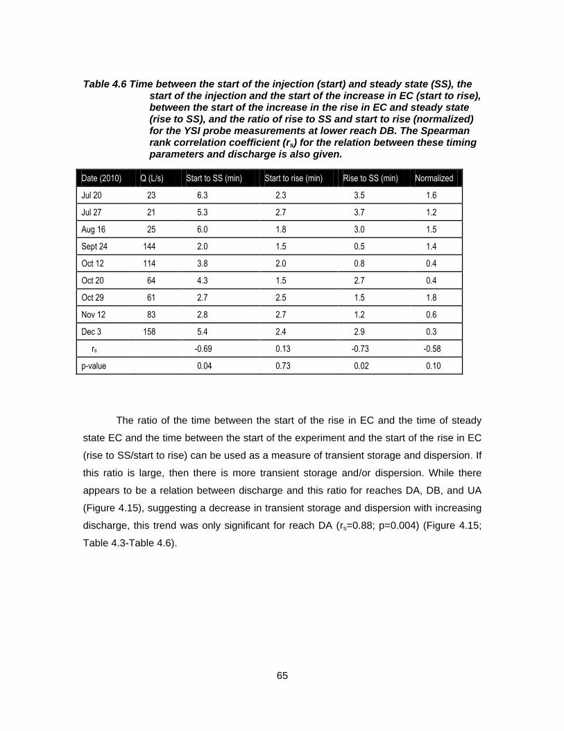
65

Table 4.6 Time between the start of the injection (start) and steady state (SS), the start of the injection and the start of the increase in EC (start to rise), between the start of the increase in the rise in EC and steady state (rise to SS), and the ratio of rise to SS and start to rise (normalized) for the YSI probe measurements at lower reach DB. The Spearman rank correlation coefficient (rs) for the relation between these timing parameters and discharge is also given.

Date (2010) Q (L/s) Start to SS (min) Start to rise (min) Rise to SS (min) Normalized

Jul 20 23 6.3 2.3 3.5 1.6

Jul 27 21 5.3 2.7 3.7 1.2

Aug 16 25 6.0 1.8 3.0 1.5

Sept 24 144 2.0 1.5 0.5 1.4

Oct 12 114 3.8 2.0 0.8 0.4

Oct 20 64 4.3 1.5 2.7 0.4

Oct 29 61 2.7 2.5 1.5 1.8

Nov 12 83 2.8 2.7 1.2 0.6

Dec 3 158 5.4 2.4 2.9 0.3

rs -0.69 0.13 -0.73 -0.58

p-value 0.04 0.73 0.02 0.10

The ratio of the time between the start of the rise in EC and the time of steady

state EC and the time between the start of the experiment and the start of the rise in EC

(rise to SS/start to rise) can be used as a measure of transient storage and dispersion. If

this ratio is large, then there is more transient storage and/or dispersion. While there

appears to be a relation between discharge and this ratio for reaches DA, DB, and UA

(Figure 4.15), suggesting a decrease in transient storage and dispersion with increasing

discharge, this trend was only significant for reach DA (rs=0.88; p=0.004) (Figure 4.15;

Table 4.3-Table 4.6).

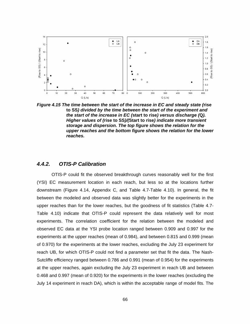
66

Figure 4.15 The time between the start of the increase in EC and steady state (rise to SS) divided by the time between the start of the experiment and the start of the increase in EC (start to rise) versus discharge (Q). Higher values of (rise to SS)/(Start to rise) indicate more transient storage and dispersion. The top figure shows the relation for the upper reaches and the bottom figure shows the relation for the lower reaches.

4.4.2. OTIS-P Calibration

OTIS-P could fit the observed breakthrough curves reasonably well for the first

(YSI) EC measurement location in each reach, but less so at the locations further

downstream (Figure 4.14, Appendix C, and Table 4.7-Table 4.10). In general, the fit

between the modeled and observed data was slightly better for the experiments in the

upper reaches than for the lower reaches, but the goodness of fit statistics (Table 4.7-

Table 4.10) indicate that OTIS-P could represent the data relatively well for most

experiments. The correlation coefficient for the relation between the modeled and

observed EC data at the YSI probe location ranged between 0.909 and 0.997 for the

experiments at the upper reaches (mean of 0.984), and between 0.815 and 0.999 (mean

of 0.970) for the experiments at the lower reaches, excluding the July 23 experiment for

reach UB, for which OTIS-P could not find a parameter set that fit the data. The Nash-

Sutcliffe efficiency ranged between 0.786 and 0.991 (mean of 0.954) for the experiments

at the upper reaches, again excluding the July 23 experiment in reach UB and between

0.468 and 0.997 (mean of 0.920) for the experiments in the lower reaches (excluding the

July 14 experiment in reach DA), which is within the acceptable range of model fits. The

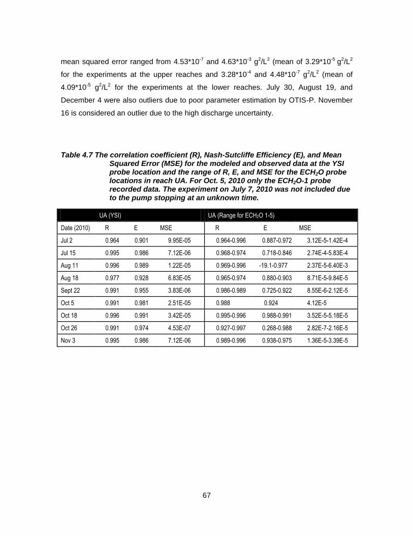
67

mean squared error ranged from 4.53*10-7 and 4.63*10-3 g2/L2 (mean of 3.29*10-5 g2/L2

for the experiments at the upper reaches and 3.28*10-4 and 4.48*10-7 g2/L2 (mean of

4.09*10-5 g2/L2 for the experiments at the lower reaches. July 30, August 19, and

December 4 were also outliers due to poor parameter estimation by OTIS-P. November

16 is considered an outlier due to the high discharge uncertainty.

Table 4.7 The correlation coefficient (R), Nash-Sutcliffe Efficiency (E), and Mean Squared Error (MSE) for the modeled and observed data at the YSI probe location and the range of R, E, and MSE for the ECH2O probe locations in reach UA. For Oct. 5, 2010 only the ECH2O-1 probe recorded data. The experiment on July 7, 2010 was not included due to the pump stopping at an unknown time.

UA (YSI) UA (Range for ECH2O 1-5)

Date (2010) R E MSE R E MSE

Jul 2 0.964 0.901 9.95E-05 0.964-0.996 0.887-0.972 3.12E-5-1.42E-4

Jul 15 0.995 0.986 7.12E-06 0.968-0.974 0.718-0.846 2.74E-4-5.83E-4

Aug 11 0.996 0.989 1.22E-05 0.969-0.996 -19.1-0.977 2.37E-5-6.40E-3

Aug 18 0.977 0.928 6.83E-05 0.965-0.974 0.880-0.903 8.71E-5-9.84E-5

Sept 22 0.991 0.955 3.83E-06 0.986-0.989 0.725-0.922 8.55E-6-2.12E-5

Oct 5 0.991 0.981 2.51E-05 0.988 0.924 4.12E-5

Oct 18 0.996 0.991 3.42E-05 0.995-0.996 0.988-0.991 3.52E-5-5.18E-5

Oct 26 0.991 0.974 4.53E-07 0.927-0.997 0.268-0.988 2.82E-7-2.16E-5

Nov 3 0.995 0.986 7.12E-06 0.989-0.996 0.938-0.975 1.36E-5-3.39E-5

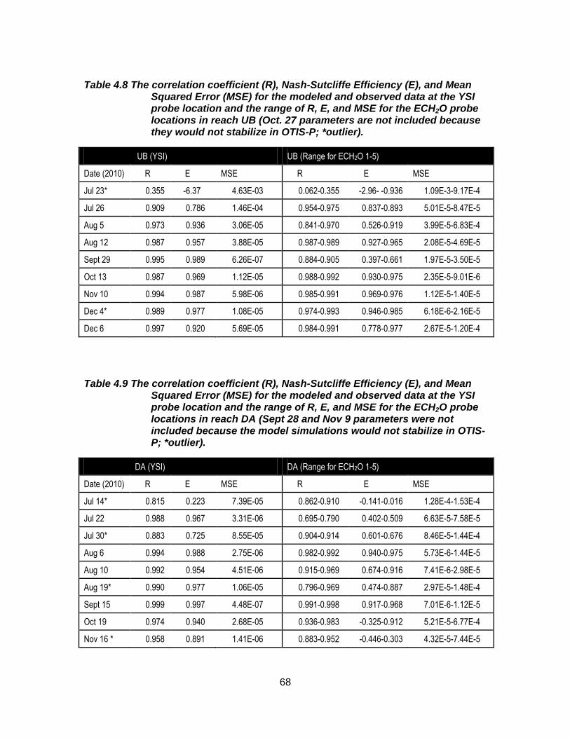
68

Table 4.8 The correlation coefficient (R), Nash-Sutcliffe Efficiency (E), and Mean Squared Error (MSE) for the modeled and observed data at the YSI probe location and the range of R, E, and MSE for the ECH2O probe locations in reach UB (Oct. 27 parameters are not included because they would not stabilize in OTIS-P; *outlier).

UB (YSI) UB (Range for ECH2O 1-5)

Date (2010) R E MSE R E MSE

Jul 23* 0.355 -6.37 4.63E-03 0.062-0.355 -2.96- -0.936 1.09E-3-9.17E-4

Jul 26 0.909 0.786 1.46E-04 0.954-0.975 0.837-0.893 5.01E-5-8.47E-5

Aug 5 0.973 0.936 3.06E-05 0.841-0.970 0.526-0.919 3.99E-5-6.83E-4

Aug 12 0.987 0.957 3.88E-05 0.987-0.989 0.927-0.965 2.08E-5-4.69E-5

Sept 29 0.995 0.989 6.26E-07 0.884-0.905 0.397-0.661 1.97E-5-3.50E-5

Oct 13 0.987 0.969 1.12E-05 0.988-0.992 0.930-0.975 2.35E-5-9.01E-6

Nov 10 0.994 0.987 5.98E-06 0.985-0.991 0.969-0.976 1.12E-5-1.40E-5

Dec 4* 0.989 0.977 1.08E-05 0.974-0.993 0.946-0.985 6.18E-6-2.16E-5

Dec 6 0.997 0.920 5.69E-05 0.984-0.991 0.778-0.977 2.67E-5-1.20E-4

Table 4.9 The correlation coefficient (R), Nash-Sutcliffe Efficiency (E), and Mean Squared Error (MSE) for the modeled and observed data at the YSI probe location and the range of R, E, and MSE for the ECH2O probe locations in reach DA (Sept 28 and Nov 9 parameters were not included because the model simulations would not stabilize in OTIS-P; *outlier).

DA (YSI) DA (Range for ECH2O 1-5)

Date (2010) R E MSE R E MSE

Jul 14* 0.815 0.223 7.39E-05 0.862-0.910 -0.141-0.016 1.28E-4-1.53E-4

Jul 22 0.988 0.967 3.31E-06 0.695-0.790 0.402-0.509 6.63E-5-7.58E-5

Jul 30* 0.883 0.725 8.55E-05 0.904-0.914 0.601-0.676 8.46E-5-1.44E-4

Aug 6 0.994 0.988 2.75E-06 0.982-0.992 0.940-0.975 5.73E-6-1.44E-5

Aug 10 0.992 0.954 4.51E-06 0.915-0.969 0.674-0.916 7.41E-6-2.98E-5

Aug 19* 0.990 0.977 1.06E-05 0.796-0.969 0.474-0.887 2.97E-5-1.48E-4

Sept 15 0.999 0.997 4.48E-07 0.991-0.998 0.917-0.968 7.01E-6-1.12E-5

Oct 19 0.974 0.940 2.68E-05 0.936-0.983 -0.325-0.912 5.21E-5-6.77E-4

Nov 16 * 0.958 0.891 1.41E-06 0.883-0.952 -0.446-0.303 4.32E-5-7.44E-5

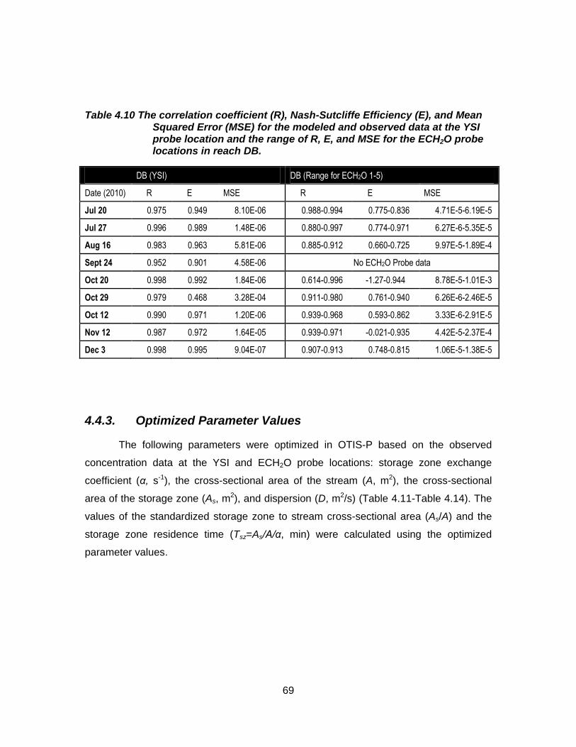
69

Table 4.10 The correlation coefficient (R), Nash-Sutcliffe Efficiency (E), and Mean Squared Error (MSE) for the modeled and observed data at the YSI probe location and the range of R, E, and MSE for the ECH2O probe locations in reach DB.

DB (YSI) DB (Range for ECH2O 1-5)

Date (2010) R E MSE R E MSE

Jul 20 0.975 0.949 8.10E-06 0.988-0.994 0.775-0.836 4.71E-5-6.19E-5

Jul 27 0.996 0.989 1.48E-06 0.880-0.997 0.774-0.971 6.27E-6-5.35E-5

Aug 16 0.983 0.963 5.81E-06 0.885-0.912 0.660-0.725 9.97E-5-1.89E-4

Sept 24 0.952 0.901 4.58E-06 No ECH2O Probe data

Oct 20 0.998 0.992 1.84E-06 0.614-0.996 -1.27-0.944 8.78E-5-1.01E-3

Oct 29 0.979 0.468 3.28E-04 0.911-0.980 0.761-0.940 6.26E-6-2.46E-5

Oct 12 0.990 0.971 1.20E-06 0.939-0.968 0.593-0.862 3.33E-6-2.91E-5

Nov 12 0.987 0.972 1.64E-05 0.939-0.971 -0.021-0.935 4.42E-5-2.37E-4

Dec 3 0.998 0.995 9.04E-07 0.907-0.913 0.748-0.815 1.06E-5-1.38E-5

4.4.3. Optimized Parameter Values

The following parameters were optimized in OTIS-P based on the observed

concentration data at the YSI and ECH2O probe locations: storage zone exchange

coefficient (α, s-1), the cross-sectional area of the stream (A, m2), the cross-sectional

area of the storage zone (As, m2), and dispersion (D, m2/s) (Table 4.11-Table 4.14). The

values of the standardized storage zone to stream cross-sectional area (As/A) and the

storage zone residence time (Tsz=As/A/α, min) were calculated using the optimized

parameter values.

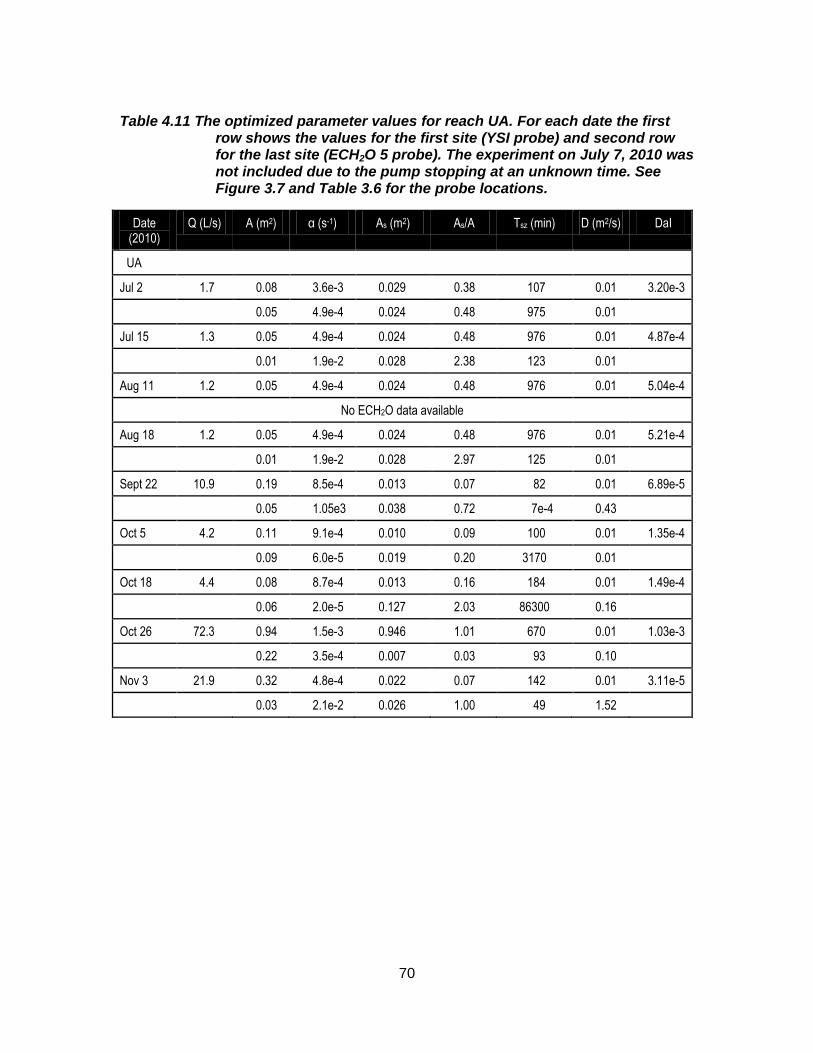
70

Table 4.11 The optimized parameter values for reach UA. For each date the first row shows the values for the first site (YSI probe) and second row for the last site (ECH2O 5 probe). The experiment on July 7, 2010 was not included due to the pump stopping at an unknown time. See Figure 3.7 and Table 3.6 for the probe locations.

Date (2010)

Q (L/s) A (m2) α (s-1) As (m2) As/A Tsz (min) D (m2/s) DaI

UA

Jul 2 1.7 0.08 3.6e-3 0.029 0.38 107 0.01 3.20e-3

0.05 4.9e-4 0.024 0.48 975 0.01

Jul 15 1.3 0.05 4.9e-4 0.024 0.48 976 0.01 4.87e-4

0.01 1.9e-2 0.028 2.38 123 0.01

Aug 11 1.2 0.05 4.9e-4 0.024 0.48 976 0.01 5.04e-4

No ECH2O data available

Aug 18 1.2 0.05 4.9e-4 0.024 0.48 976 0.01 5.21e-4

0.01 1.9e-2 0.028 2.97 125 0.01

Sept 22 10.9 0.19 8.5e-4 0.013 0.07 82 0.01 6.89e-5

0.05 1.05e3 0.038 0.72 7e-4 0.43

Oct 5 4.2 0.11 9.1e-4 0.010 0.09 100 0.01 1.35e-4

0.09 6.0e-5 0.019 0.20 3170 0.01

Oct 18 4.4 0.08 8.7e-4 0.013 0.16 184 0.01 1.49e-4

0.06 2.0e-5 0.127 2.03 86300 0.16

Oct 26 72.3 0.94 1.5e-3 0.946 1.01 670 0.01 1.03e-3

0.22 3.5e-4 0.007 0.03 93 0.10

Nov 3 21.9 0.32 4.8e-4 0.022 0.07 142 0.01 3.11e-5

0.03 2.1e-2 0.026 1.00 49 1.52

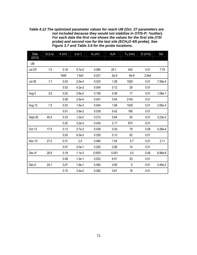
71

Table 4.12 The optimized parameter values for reach UB (Oct. 27 parameters are not included because they would not stabilize in OTIS-P; *outlier). For each date the first row shows the values for the first site (YSI probe) and second row for the last site (ECH2O 4/5 probe). See Figure 3.7 and Table 3.6 for the probe locations.

Date (2010)

Q (L/s) A (m2) α (s-1) As (m2) As/A Tsz (min) D (m2/s) DaI

UB

Jul 23* 1.5 0.16 5.7e-2 4.090 25.1 442 0.01 7.75

1606 1.6e3 0.021 2e-5 9e-9 2.9e4

Jul 26 1.7 0.03 2.5e-4 0.033 1.28 1920 0.01 7.59e-4

0.03 4.2e-3 0.004 0.12 29 0.01

Aug 5 3.6 0.02 2.8e-2 0.108 0.48 17 0.01 1.08e-1

0.08 2.5e-4 0.041 0.54 2140 0.01

Aug 12 1.5 0.03 1.6e-3 0.054 1.68 1030 0.01 3.06e-3

0.01 3.9e-2 0.039 6.42 166 0.01

Sept 29 40.4 0.33 1.2e-2 0.213 0.64 54 0.01 3.23e-3

0.20 3.2e-3 0.434 2.17 674 0.01

Oct 13 17.9 0.13 3.7e-3 0.039 0.30 79 0.08 4.28e-4

0.05 8.3e-2 0.255 5.13 62 0.01

Nov 10 27.2 0.31 2.4 0.484 1.54 0.7 0.01 2.11

0.07 2.0e-1 0.200 2.86 14 0.01

Dec 4* 28.9 0.18 1.1e-3 0.0001 0.001 0.5 0.06 6.96e-6

0.08 1.2e-1 0.522 6.51 53 0.01

Dec 6 24.7 0.07 1.9e-1 0.064 0.85 5 0.01 2.45e-2

0.15 3.4e-2 0.092 0.61 18 0.01

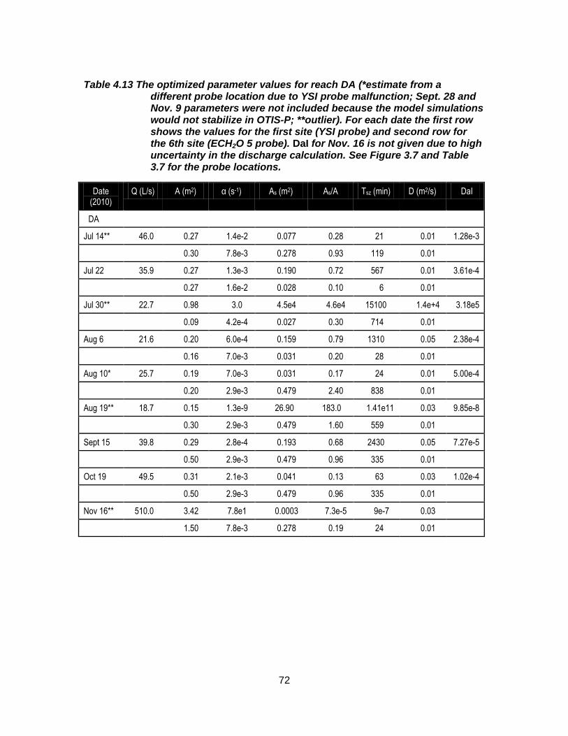
72

Table 4.13 The optimized parameter values for reach DA (*estimate from a different probe location due to YSI probe malfunction; Sept. 28 and Nov. 9 parameters were not included because the model simulations would not stabilize in OTIS-P; **outlier). For each date the first row shows the values for the first site (YSI probe) and second row for the 6th site (ECH2O 5 probe). DaI for Nov. 16 is not given due to high uncertainty in the discharge calculation. See Figure 3.7 and Table 3.7 for the probe locations.

Date (2010)

Q (L/s) A (m2) α (s-1) As (m2) As/A Tsz (min) D (m2/s) DaI

DA

Jul 14** 46.0 0.27 1.4e-2 0.077 0.28 21 0.01 1.28e-3

0.30 7.8e-3 0.278 0.93 119 0.01

Jul 22 35.9 0.27 1.3e-3 0.190 0.72 567 0.01 3.61e-4

0.27 1.6e-2 0.028 0.10 6 0.01

Jul 30** 22.7 0.98 3.0 4.5e4 4.6e4 15100 1.4e+4 3.18e5

0.09 4.2e-4 0.027 0.30 714 0.01

Aug 6 21.6 0.20 6.0e-4 0.159 0.79 1310 0.05 2.38e-4

0.16 7.0e-3 0.031 0.20 28 0.01

Aug 10* 25.7 0.19 7.0e-3 0.031 0.17 24 0.01 5.00e-4

0.20 2.9e-3 0.479 2.40 838 0.01

Aug 19** 18.7 0.15 1.3e-9 26.90 183.0 1.41e11 0.03 9.85e-8

0.30 2.9e-3 0.479 1.60 559 0.01

Sept 15 39.8 0.29 2.8e-4 0.193 0.68 2430 0.05 7.27e-5

0.50 2.9e-3 0.479 0.96 335 0.01

Oct 19 49.5 0.31 2.1e-3 0.041 0.13 63 0.03 1.02e-4

0.50 2.9e-3 0.479 0.96 335 0.01

Nov 16** 510.0 3.42 7.8e1 0.0003 7.3e-5 9e-7 0.03

1.50 7.8e-3 0.278 0.19 24 0.01

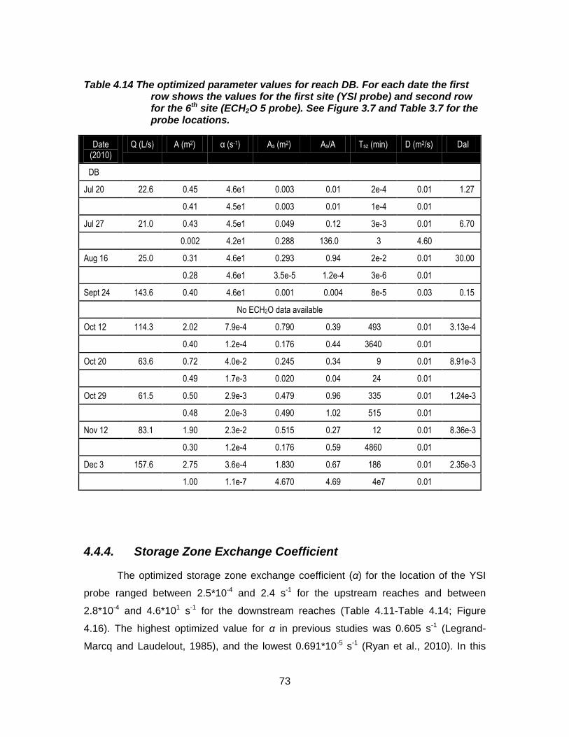
73

Table 4.14 The optimized parameter values for reach DB. For each date the first row shows the values for the first site (YSI probe) and second row for the 6th site (ECH2O 5 probe). See Figure 3.7 and Table 3.7 for the probe locations.

Date (2010)

Q (L/s) A (m2) α (s-1) As (m2) As/A Tsz (min) D (m2/s) DaI

DB

Jul 20 22.6 0.45 4.6e1 0.003 0.01 2e-4 0.01 1.27

0.41 4.5e1 0.003 0.01 1e-4 0.01

Jul 27 21.0 0.43 4.5e1 0.049 0.12 3e-3 0.01 6.70

0.002 4.2e1 0.288 136.0 3 4.60

Aug 16 25.0 0.31 4.6e1 0.293 0.94 2e-2 0.01 30.00

0.28 4.6e1 3.5e-5 1.2e-4 3e-6 0.01

Sept 24 143.6 0.40 4.6e1 0.001 0.004 8e-5 0.03 0.15

No ECH2O data available

Oct 12 114.3 2.02 7.9e-4 0.790 0.39 493 0.01 3.13e-4

0.40 1.2e-4 0.176 0.44 3640 0.01

Oct 20 63.6 0.72 4.0e-2 0.245 0.34 9 0.01 8.91e-3

0.49 1.7e-3 0.020 0.04 24 0.01

Oct 29 61.5 0.50 2.9e-3 0.479 0.96 335 0.01 1.24e-3

0.48 2.0e-3 0.490 1.02 515 0.01

Nov 12 83.1 1.90 2.3e-2 0.515 0.27 12 0.01 8.36e-3

0.30 1.2e-4 0.176 0.59 4860 0.01

Dec 3 157.6 2.75 3.6e-4 1.830 0.67 186 0.01 2.35e-3

1.00 1.1e-7 4.670 4.69 4e7 0.01

4.4.4. Storage Zone Exchange Coefficient

The optimized storage zone exchange coefficient (α) for the location of the YSI

probe ranged between 2.5*10-4 and 2.4 s-1 for the upstream reaches and between

2.8*10-4 and 4.6*101 s-1 for the downstream reaches (Table 4.11-Table 4.14; Figure

4.16). The highest optimized value for α in previous studies was 0.605 s-1 (Legrand-

Marcq and Laudelout, 1985), and the lowest 0.691*10-5 s-1 (Ryan et al., 2010). In this

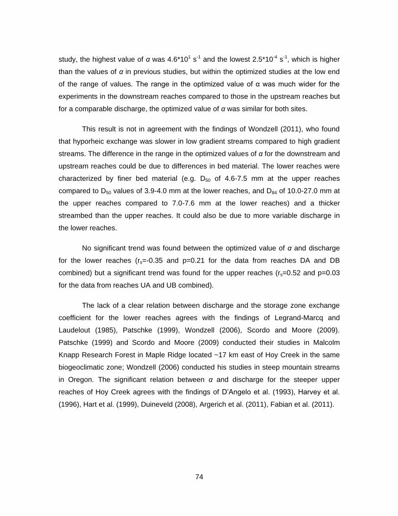
74

study, the highest value of α was 4.6*101 s-1 and the lowest 2.5*10-4 s-1, which is higher

than the values of α in previous studies, but within the optimized studies at the low end

of the range of values. The range in the optimized value of α was much wider for the

experiments in the downstream reaches compared to those in the upstream reaches but

for a comparable discharge, the optimized value of α was similar for both sites.

This result is not in agreement with the findings of Wondzell (2011), who found

that hyporheic exchange was slower in low gradient streams compared to high gradient

streams. The difference in the range in the optimized values of α for the downstream and

upstream reaches could be due to differences in bed material. The lower reaches were

characterized by finer bed material (e.g. D50 of 4.6-7.5 mm at the upper reaches

compared to D50 values of 3.9-4.0 mm at the lower reaches, and D84 of 10.0-27.0 mm at

the upper reaches compared to 7.0-7.6 mm at the lower reaches) and a thicker

streambed than the upper reaches. It could also be due to more variable discharge in

the lower reaches.

No significant trend was found between the optimized value of α and discharge

for the lower reaches (rs=-0.35 and p=0.21 for the data from reaches DA and DB

combined) but a significant trend was found for the upper reaches (rs=0.52 and p=0.03

for the data from reaches UA and UB combined).

The lack of a clear relation between discharge and the storage zone exchange

coefficient for the lower reaches agrees with the findings of Legrand-Marcq and

Laudelout (1985), Patschke (1999), Wondzell (2006), Scordo and Moore (2009).

Patschke (1999) and Scordo and Moore (2009) conducted their studies in Malcolm

Knapp Research Forest in Maple Ridge located ~17 km east of Hoy Creek in the same

biogeoclimatic zone; Wondzell (2006) conducted his studies in steep mountain streams

in Oregon. The significant relation between α and discharge for the steeper upper

reaches of Hoy Creek agrees with the findings of D’Angelo et al. (1993), Harvey et al.

(1996), Hart et al. (1999), Duineveld (2008), Argerich et al. (2011), Fabian et al. (2011).

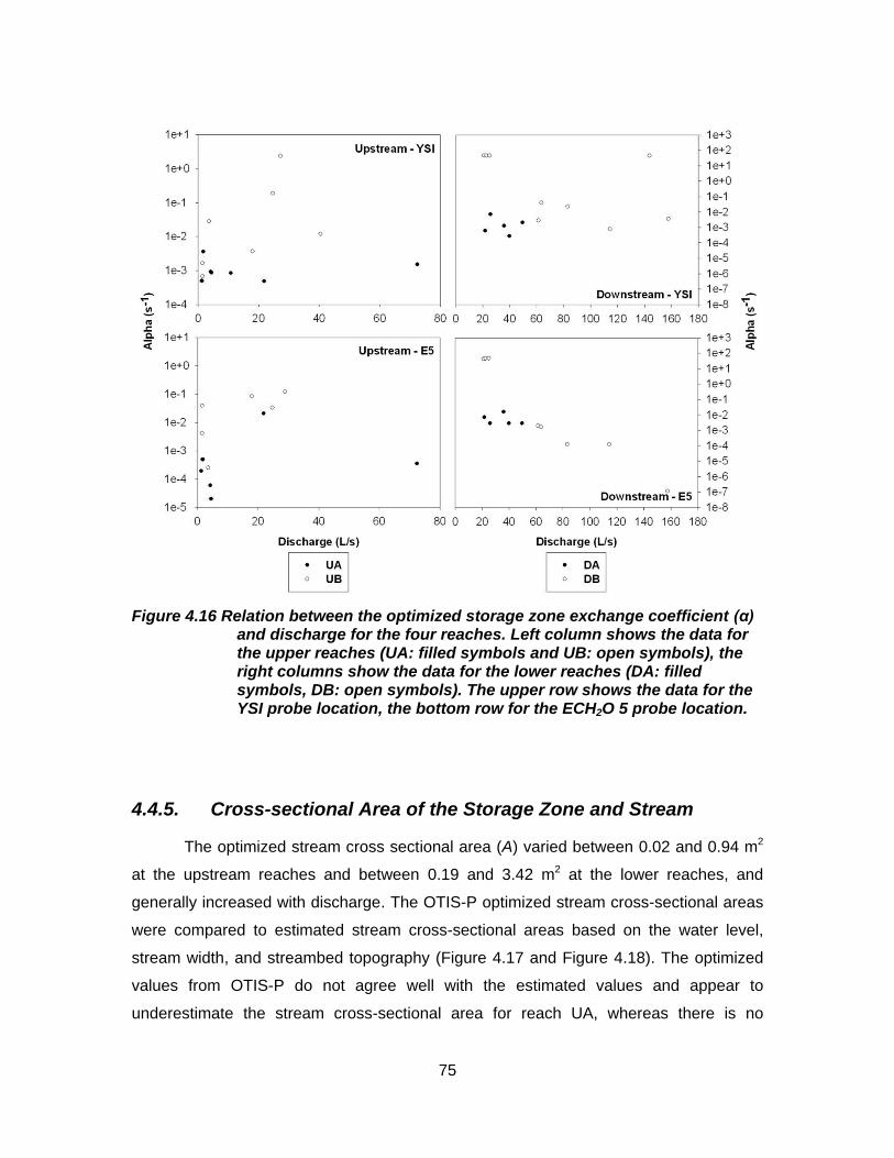
75

Figure 4.16 Relation between the optimized storage zone exchange coefficient (α) and discharge for the four reaches. Left column shows the data for the upper reaches (UA: filled symbols and UB: open symbols), the right columns show the data for the lower reaches (DA: filled symbols, DB: open symbols). The upper row shows the data for the YSI probe location, the bottom row for the ECH2O 5 probe location.

4.4.5. Cross-sectional Area of the Storage Zone and Stream

The optimized stream cross sectional area (A) varied between 0.02 and 0.94 m2

at the upstream reaches and between 0.19 and 3.42 m2 at the lower reaches, and

generally increased with discharge. The OTIS-P optimized stream cross-sectional areas

were compared to estimated stream cross-sectional areas based on the water level,

stream width, and streambed topography (Figure 4.17 and Figure 4.18). The optimized

values from OTIS-P do not agree well with the estimated values and appear to

underestimate the stream cross-sectional area for reach UA, whereas there is no

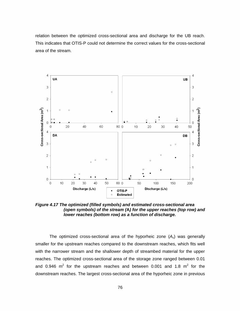
76

relation between the optimized cross-sectional area and discharge for the UB reach.

This indicates that OTIS-P could not determine the correct values for the cross-sectional

area of the stream.

Figure 4.17 The optimized (filled symbols) and estimated cross-sectional area (open symbols) of the stream (A) for the upper reaches (top row) and lower reaches (bottom row) as a function of discharge.

The optimized cross-sectional area of the hyporheic zone (As) was generally

smaller for the upstream reaches compared to the downstream reaches, which fits well

with the narrower stream and the shallower depth of streambed material for the upper

reaches. The optimized cross-sectional area of the storage zone ranged between 0.01

and 0.946 m2 for the upstream reaches and between 0.001 and 1.8 m2 for the

downstream reaches. The largest cross-sectional area of the hyporheic zone in previous

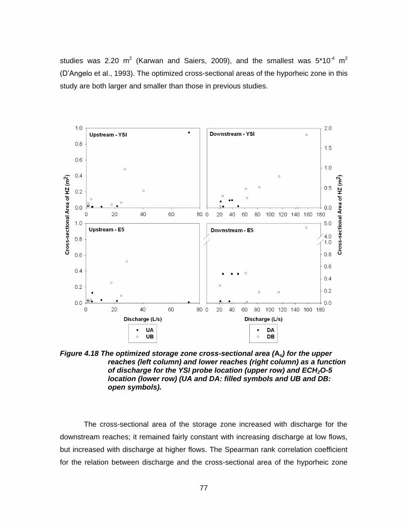
77

studies was 2.20 m2 (Karwan and Saiers, 2009), and the smallest was 5*10-4 m2

(D’Angelo et al., 1993). The optimized cross-sectional areas of the hyporheic zone in this

study are both larger and smaller than those in previous studies.

Figure 4.18 The optimized storage zone cross-sectional area (As) for the upper reaches (left column) and lower reaches (right column) as a function of discharge for the YSI probe location (upper row) and ECH2O-5 location (lower row) (UA and DA: filled symbols and UB and DB: open symbols).

The cross-sectional area of the storage zone increased with discharge for the

downstream reaches; it remained fairly constant with increasing discharge at low flows,

but increased with discharge at higher flows. The Spearman rank correlation coefficient

for the relation between discharge and the cross-sectional area of the hyporheic zone

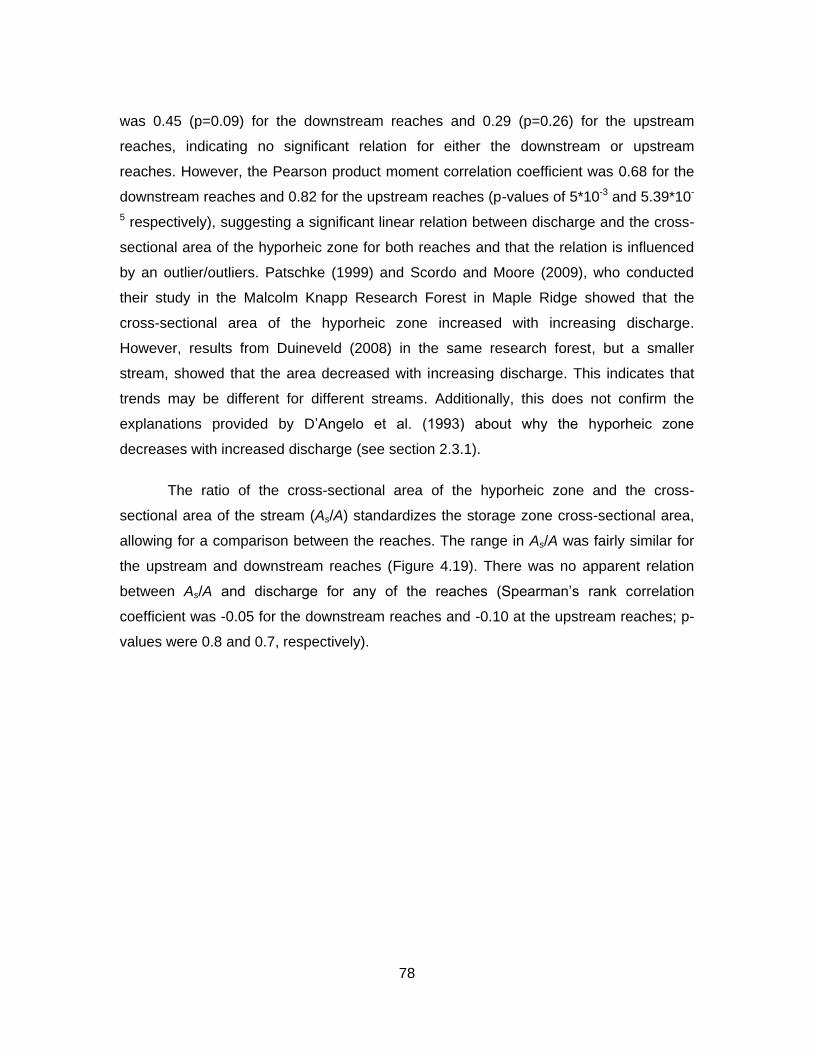
78

was 0.45 (p=0.09) for the downstream reaches and 0.29 (p=0.26) for the upstream

reaches, indicating no significant relation for either the downstream or upstream

reaches. However, the Pearson product moment correlation coefficient was 0.68 for the

downstream reaches and 0.82 for the upstream reaches (p-values of 5*10-3 and 5.39*10-

5 respectively), suggesting a significant linear relation between discharge and the cross-

sectional area of the hyporheic zone for both reaches and that the relation is influenced

by an outlier/outliers. Patschke (1999) and Scordo and Moore (2009), who conducted

their study in the Malcolm Knapp Research Forest in Maple Ridge showed that the

cross-sectional area of the hyporheic zone increased with increasing discharge.

However, results from Duineveld (2008) in the same research forest, but a smaller

stream, showed that the area decreased with increasing discharge. This indicates that

trends may be different for different streams. Additionally, this does not confirm the

explanations provided by D’Angelo et al. (1993) about why the hyporheic zone

decreases with increased discharge (see section 2.3.1).

The ratio of the cross-sectional area of the hyporheic zone and the cross-

sectional area of the stream (As/A) standardizes the storage zone cross-sectional area,

allowing for a comparison between the reaches. The range in As/A was fairly similar for

the upstream and downstream reaches (Figure 4.19). There was no apparent relation

between As/A and discharge for any of the reaches (Spearman’s rank correlation

coefficient was -0.05 for the downstream reaches and -0.10 at the upstream reaches; p-

values were 0.8 and 0.7, respectively).

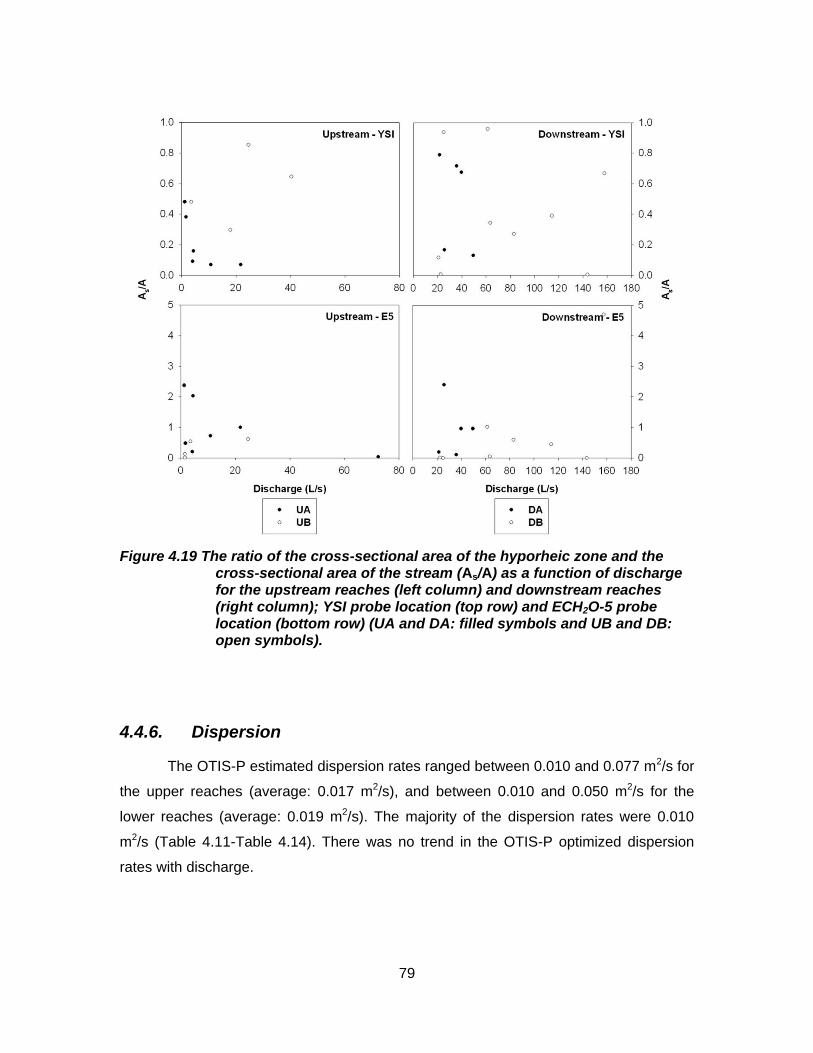
79

Figure 4.19 The ratio of the cross-sectional area of the hyporheic zone and the cross-sectional area of the stream (As/A) as a function of discharge for the upstream reaches (left column) and downstream reaches (right column); YSI probe location (top row) and ECH2O-5 probe location (bottom row) (UA and DA: filled symbols and UB and DB: open symbols).

4.4.6. Dispersion

The OTIS-P estimated dispersion rates ranged between 0.010 and 0.077 m2/s for

the upper reaches (average: 0.017 m2/s), and between 0.010 and 0.050 m2/s for the

lower reaches (average: 0.019 m2/s). The majority of the dispersion rates were 0.010

m2/s (Table 4.11-Table 4.14). There was no trend in the OTIS-P optimized dispersion

rates with discharge.

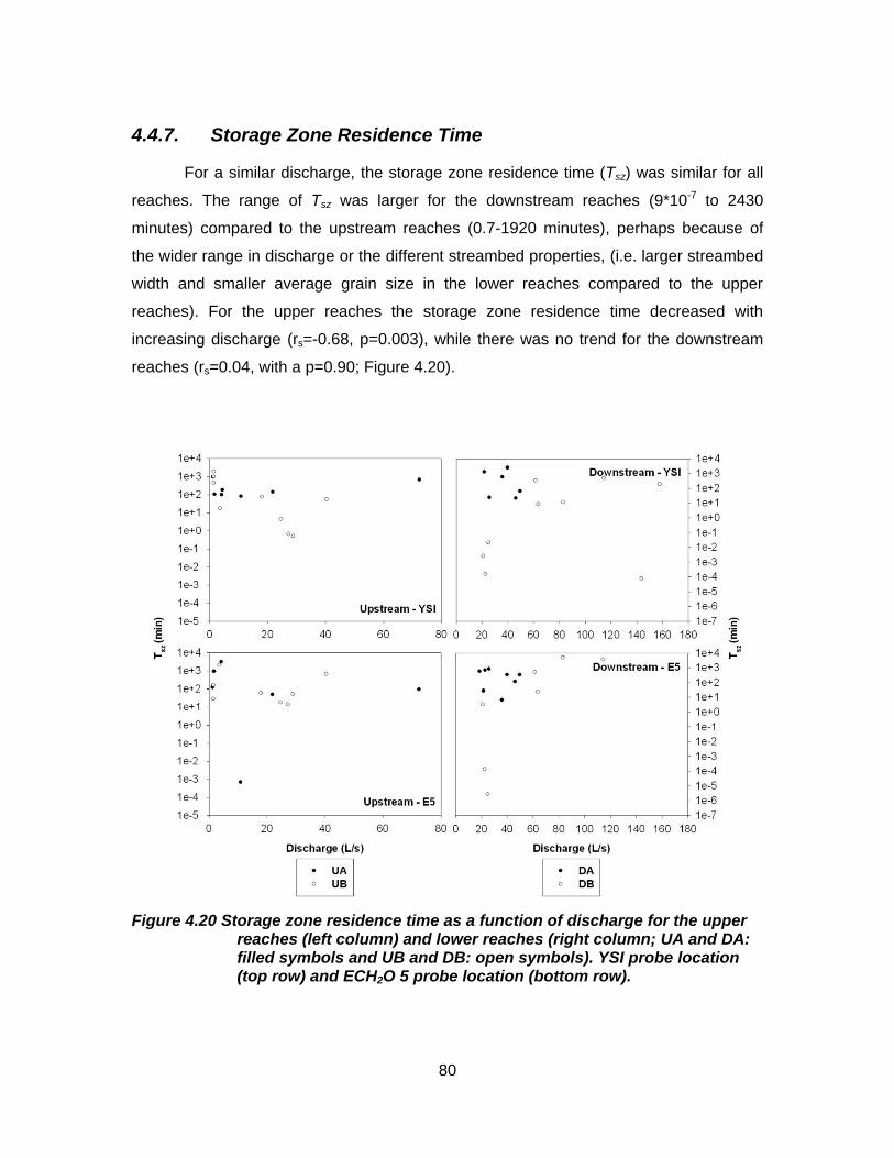
80

4.4.7. Storage Zone Residence Time

For a similar discharge, the storage zone residence time (Tsz) was similar for all

reaches. The range of Tsz was larger for the downstream reaches (9*10-7 to 2430

minutes) compared to the upstream reaches (0.7-1920 minutes), perhaps because of

the wider range in discharge or the different streambed properties, (i.e. larger streambed

width and smaller average grain size in the lower reaches compared to the upper

reaches). For the upper reaches the storage zone residence time decreased with

increasing discharge (rs=-0.68, p=0.003), while there was no trend for the downstream

reaches (rs=0.04, with a p=0.90; Figure 4.20).

Figure 4.20 Storage zone residence time as a function of discharge for the upper reaches (left column) and lower reaches (right column; UA and DA: filled symbols and UB and DB: open symbols). YSI probe location (top row) and ECH2O 5 probe location (bottom row).

81

4.4.8. Hydraulic Retention Factor and Average Traveling Distance of a Water Molecule

The hydraulic retention factor (Rh=As/Q) varied between 1.0 and 37.4 s/m at the

upper reaches, and between 4.9*10-4 and 11.7 s/m at the lower reaches (Figure 4.21).

There was a significant relation between Rh and discharge for the upper reaches (rs=-

0.59, p=0.015) but not for the lower reaches (rs=0.11, p=0.71).

Figure 4.21 Hydraulic retention factor (Rh) as a function of discharge at the YSI probe location (UA and DA: filled symbols and UB and DB: open symbols).

The average distance a water molecule travels in the stream before entering

transient storage (Ls=Q/A/α) varied between 0.6 and 144 m at the upper reaches, and

between 1.1*10-3 and 503 m at the lower reaches (Figure 4.22). There was no significant

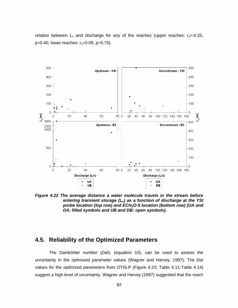
82

relation between Ls and discharge for any of the reaches (upper reaches: rs=-0.20,

p=0.45; lower reaches: rs=0.09, p=0.75).

Figure 4.22 The average distance a water molecule travels in the stream before entering transient storage (Ls) as a function of discharge at the YSI probe location (top row) and ECH2O-5 location (bottom row) (UA and DA: filled symbols and UB and DB: open symbols).

4.5. Reliability of the Optimized Parameters

The Damköhler number (DaI), (equation 10), can be used to assess the

uncertainty in the optimized parameter values (Wagner and Harvey, 1997). The DaI

values for the optimized parameters from OTIS-P (Figure 4.23; Table 4.11-Table 4.14)

suggest a high level of uncertainty. Wagner and Harvey (1997) suggested that the reach

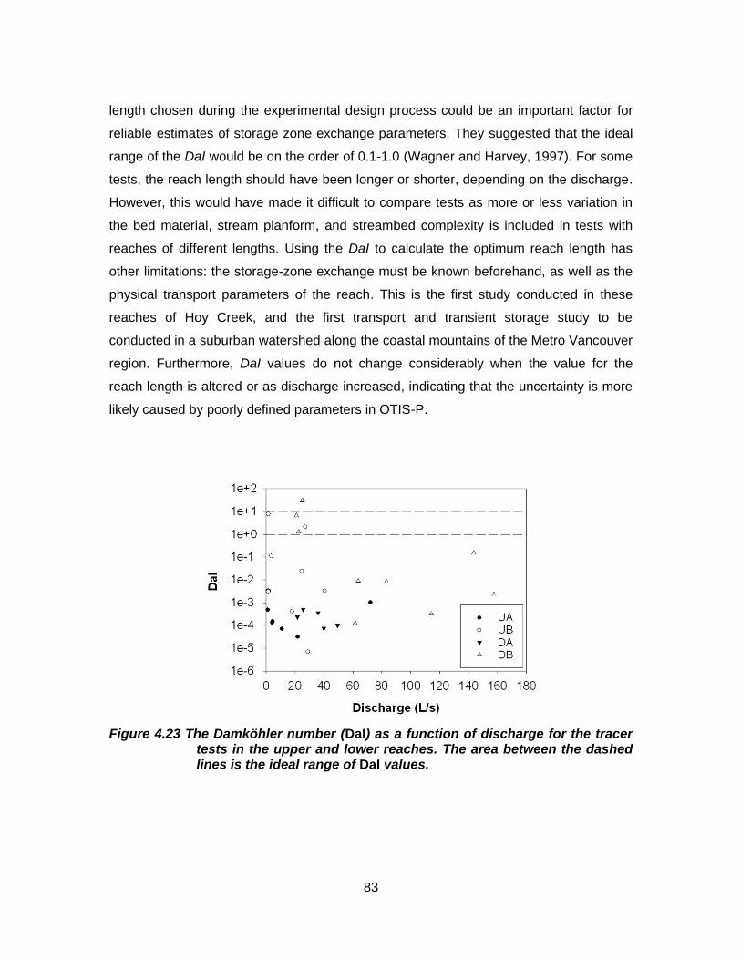
83

length chosen during the experimental design process could be an important factor for

reliable estimates of storage zone exchange parameters. They suggested that the ideal

range of the DaI would be on the order of 0.1-1.0 (Wagner and Harvey, 1997). For some

tests, the reach length should have been longer or shorter, depending on the discharge.

However, this would have made it difficult to compare tests as more or less variation in

the bed material, stream planform, and streambed complexity is included in tests with

reaches of different lengths. Using the DaI to calculate the optimum reach length has

other limitations: the storage-zone exchange must be known beforehand, as well as the

physical transport parameters of the reach. This is the first study conducted in these

reaches of Hoy Creek, and the first transport and transient storage study to be

conducted in a suburban watershed along the coastal mountains of the Metro Vancouver

region. Furthermore, DaI values do not change considerably when the value for the

reach length is altered or as discharge increased, indicating that the uncertainty is more

likely caused by poorly defined parameters in OTIS-P.

Figure 4.23 The Damköhler number (DaI) as a function of discharge for the tracer tests in the upper and lower reaches. The area between the dashed lines is the ideal range of DaI values.

84

4.6. Model Validation

Validation of OTIS was done by using the optimized parameter values from

OTIS-P to model the concentrations at the DEC probes and in the piezometers in OTIS.

The modeled results were compared with the observed data to determine how well OTIS

predicted the stream concentrations at the DEC locations and the concentrations in the

streambed. An example of the modeled and observed data is shown in Figure 4.24; all

other validation graphs can be found in Appendix D. A summary of the goodness of fit

parameters is given in Table 4.15 and Table 4.16.

The OTIS validation results indicate poor model performance for the DEC sites

and the streambed. The R, E, and MSE values indicate a much poorer fit for the DEC

and piezometer sites compared to the sites that were used in the calibration (Table 4.15

and Table 4.16). For some (15-19 out of 35) piezometers, concentration data indicated a

lack of interaction (or very slow interaction) with the stream as streambed EC did not

change significantly during the tracer test. In only a few piezometers and during a few

tests, there was a delay in the increase in concentrations during the experiment. For

reach DA, there were 3 piezometers that indicated that the tracer moved through the bed

(P9, P8, and P3). P9 is located in the bank along a straight stretch of the reach; P8 is

located within the stream at the edge of a bar along a meander bend; P3 is located in a

bar at the end of a meander bend. In reach DB, there were two piezometers that showed

that the tracer moved through the bed (P6 and P1) during higher flow events. These

piezometers are both located in a bar along a meander bend.

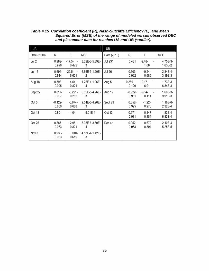
85

Table 4.15 Correlation coefficient (R), Nash-Sutcliffe Efficiency (E), and Mean Squared Error (MSE) of the range of modeled versus observed DEC and piezometer data for reaches UA and UB (*outlier).

UA UB

Date (2010) R E MSE Date (2010) R E MSE

Jul 2 0.989-0.998

-17.5- -0.472

3.32E-3-5.39E-3

Jul 23* 0.481 -2.48- -1.08

4.75E-3-1.63E-2

Jul 15 0.694-0.944

-22.5- -6.621

6.66E-3-1.20E-2

Jul 26 0.503-0.962

-9.24-0.685

2.34E-4-3.19E-3

Aug 18 0.593-0.995

-4.64-0.821

1.26E-4-1.26E-4

Aug 5 -0.289- -0.120

-9.17- -6.01

1.73E-3-6.84E-3

Sept 22 0.817-0.907

-0.221-0.262

6.62E-5-4.26E-3

Aug 12 -0.922-0.981

-27.4- -0.111

1.60E-3-9.91E-3

Oct 5 -0.122-0.860

-0.674-0.688

9.54E-5-4.26E-3

Sept 29 0.652-0.995

-1.22-0.978

1.16E-6-2.32E-4

Oct 18 0.801 -1.04 9.01E-4 Oct 13 0.971-0.981

0.147-0.184

1.83E-4-6.83E-4

Oct 26 0.887-0.973

-2.95-0.821

3.98E-6-3.60E-4

Dec 4* 0.952-0.963

0.672-0.894

2.10E-4- 5.25E-5

Nov 3 0.930-0.963

0.010-0.619

4.53E-4-1.42E-3

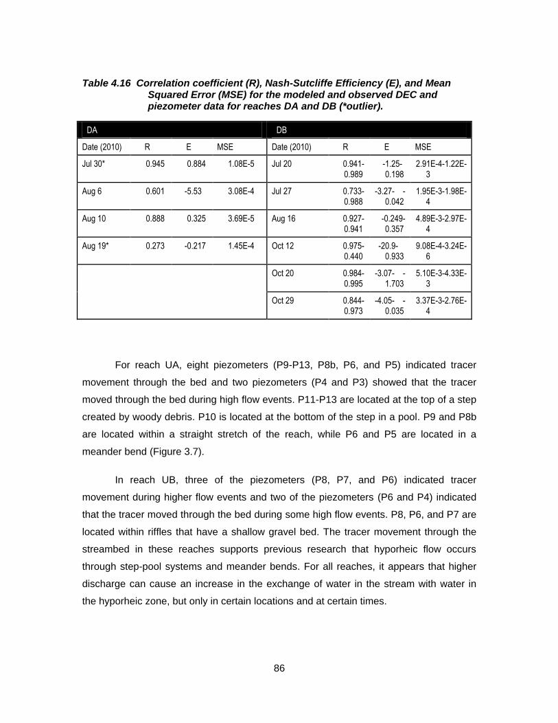
86

Table 4.16 Correlation coefficient (R), Nash-Sutcliffe Efficiency (E), and Mean Squared Error (MSE) for the modeled and observed DEC and piezometer data for reaches DA and DB (*outlier).

DA DB

Date (2010) R E MSE Date (2010) R E MSE

Jul 30* 0.945 0.884 1.08E-5 Jul 20 0.941-0.989

-1.25-0.198

2.91E-4-1.22E-3

Aug 6 0.601 -5.53 3.08E-4 Jul 27 0.733-0.988

-3.27- -0.042

1.95E-3-1.98E-4

Aug 10 0.888 0.325 3.69E-5 Aug 16 0.927-0.941

-0.249-0.357

4.89E-3-2.97E-4

Aug 19* 0.273 -0.217 1.45E-4 Oct 12 0.975-0.440

-20.9-0.933

9.08E-4-3.24E-6

Oct 20 0.984-0.995

-3.07- -1.703

5.10E-3-4.33E-3

Oct 29 0.844-0.973

-4.05- -0.035

3.37E-3-2.76E-4

For reach UA, eight piezometers (P9-P13, P8b, P6, and P5) indicated tracer

movement through the bed and two piezometers (P4 and P3) showed that the tracer

moved through the bed during high flow events. P11-P13 are located at the top of a step

created by woody debris. P10 is located at the bottom of the step in a pool. P9 and P8b

are located within a straight stretch of the reach, while P6 and P5 are located in a

meander bend (Figure 3.7).

In reach UB, three of the piezometers (P8, P7, and P6) indicated tracer

movement during higher flow events and two of the piezometers (P6 and P4) indicated

that the tracer moved through the bed during some high flow events. P8, P6, and P7 are

located within riffles that have a shallow gravel bed. The tracer movement through the

streambed in these reaches supports previous research that hyporheic flow occurs

through step-pool systems and meander bends. For all reaches, it appears that higher

discharge can cause an increase in the exchange of water in the stream with water in

the hyporheic zone, but only in certain locations and at certain times.

87

For the majority of the experiments, OTIS predicted incorrect concentrations in

the hyporheic zone. For reach UA, the observed data for piezometers P5, P6, P9, P10,

P11, P12, and P13 were fit reasonably well for only 3-4 experiments. For reach UB, only

the streambed concentrations at P4, P7, and P8 were predicted reasonably well.

Piezometer P8 was the only piezometer in reach DA for which OTIS could predict the

streambed concentrations reasonably well (R2 >0.9). For reach DB, concentrations were

not predicted well for any of the piezometers. In most cases, the model fit the data just

after the initiation of the tracer injection and after the end of the injection reasonably well

but did not accurately reflect the rise in concentration very well. The observed streambed

concentration data showed in most cases a slow exchange, if any at all, while the

modeled data predicted a fast exchange between the main channel and the storage

zones. Thus, it appears that the model overestimated the rate of hyporheic exchange.

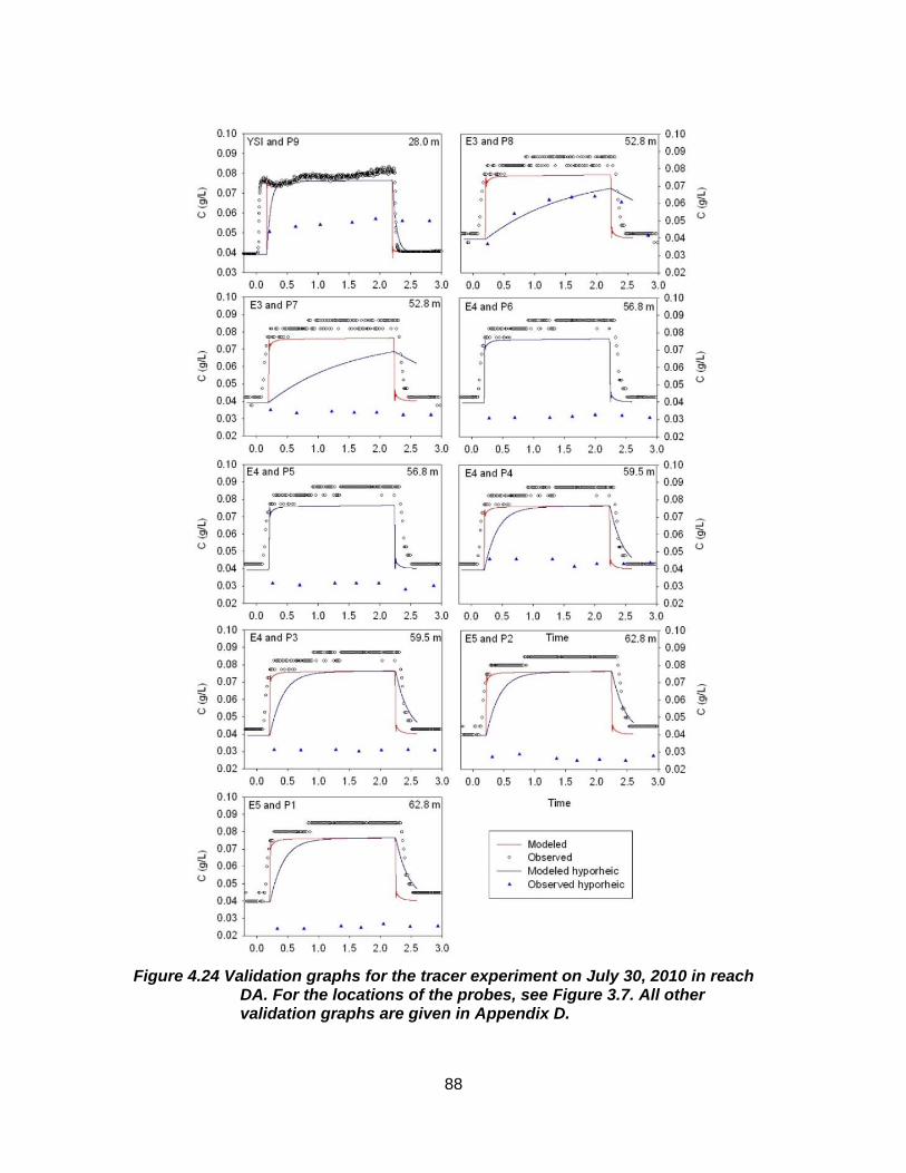
88

Figure 4.24 Validation graphs for the tracer experiment on July 30, 2010 in reach DA. For the locations of the probes, see Figure 3.7. All other validation graphs are given in Appendix D.

89

4.7. Issues with OTIS

Parameter estimation was difficult, largely due to parameter equifinality. When

running OTIS-P to optimize the A, As, D, and α parameter values, different values would

yield similar modeled concentrations and similar goodness of fit values. Ward et al.

(2012) stated that equifinality can be the result of simplification of heterogeneity within

the subsurface of the stream in a model.

Validation of the model using the DEC probe and piezometer data indicated that

the optimized parameter values did not fit the data well and that therefore the estimated

parameter values were not correct or that the model structure was wrong. In some

cases, (i.e. at 16-20 piezometers) the modeled data fit the observed data, but in other

cases they did not. The model therefore does not consistently and accurately estimate

the correct parameters.

Szeftel et al. (2011) identified a number of issues that can arise when using

transient storage models, which include (a) incorrect estimates of transient storage

parameters due to uncertainties in analyzing breakthrough curves, (b) incorrect

identification of spatial patterns of inflow and outflow, and (c) poorly defined boundary

conditions. They state that model parameterization is highly dependent on the structure

of the model. Additionally, OTIS does not incorporate streambed topography, which is a

very important aspect to consider when predicting storage zone exchange parameters

(Stondedahl et al., 2012).

Drummond et al. (2010) highlighted that the majority of stream tracer

experiments have truncated breakthrough curves. OTIS uses an exponential residence

time distribution for residence time distribution, which was found to be useful only for

stream reaches with limited storage, and therefore limited transient storage exchange.

Process-based models that incorporate hyporheic exchange as a fractal process seem

to be more appropriate for modeling hyporheic exchange because they characterize the

hyporheic residence time distribution as a power law. Additionally, OTIS tends to

underestimate hyporheic solute retention, mean travel time, dispersion, and solute

storage time as a result of truncation of the tracer experiments and overestimation of

reaction rates (Drummond et al., 2010). Ward et al. (2012) also noted that if subsurface

90

characteristics are simplified, or idealized, hyporheic exchange and residence time

distributions can be overestimated or underestimated.

91

5. Conclusion and Recommendations

5.1. Conclusion

The objective of this study was to determine how discharge, streambed

topography, and channel planform influence hyporheic exchange in a coastal suburban

stream in British Columbia. Tracer experiments were carried out in four reaches of Hoy

Creek, and the tracer breakthrough curves were modelled in OTIS to determine the

channel and storage zone cross-sectional areas, dispersion coefficient, and storage

zone exchange coefficient. However, validation of OTIS using the EC measurements in

the stream and streambed indicated poor model performance; the modeled data did not

fit the observed data well. This highlights that one must take caution when using OTIS to

estimate stream and storage zone parameters.

The optimized value of the rate of hyporheic exchange (α) was similar for the

high and low gradient reaches during comparable discharge conditions, which disagrees

with hypothesis one. The range of the rate of hyporheic exchange, however, was larger

for the lower gradient reaches due to a wider range of discharges conditions compared

to the upper higher gradient reaches. The optimized values of the storage zone

exchange coefficient were larger than expected based on previous studies. The

hyporheic zone was generally smaller for the upstream reaches compared to the

downstream reaches due to the upstream reaches being narrower and having shallower

streambed material depth. This agrees with hypothesis one.

Increasing discharge led to an increase in the rate of hyporheic exchange at the

steeper upper reaches but there was no relation between discharge and the hyporheic

exchange coefficient for the lower reaches. The tracer breakthrough curves for the

measurements in the piezometers indicated more exchange when discharge increased

as the tracer was observed in more piezometers during high flow conditions. There was

no relation between discharge and the extent of the hyporheic zone for any of the

92

reaches. These results disagree with hypothesis two as hyporheic exchange was

expected to decrease with increasing discharge and the extent of the hyporheic zone

was expected to increase with increasing discharge. Increasing discharge led to

decreased upwelling in reaches UA and DB and increased downwelling in the meander

bend in reach DA. However upwelling conditions cannot directly be related to hyporheic

exchange and may also indicate groundwater inflow.

The vertical hydraulic gradient measurements and streambed tracer movement

showed that hyporheic flow occurred through meander bends, step-pool systems, and

riffles, which is consistent with the results from previous research. Spatial variation in

hyporheic exchange, however, was considerable within each reach and between the

reaches. Streambed topography and channel planform increased hyporheic exchange;

there was increased upwelling in reaches UA and DB, and increased downwelling in

reach DA through meander bends, as well as increased upwelling and downwelling

through step-pool systems. These results support the first part of hypothesis three.

However, it remains difficult to determine whether or not this upwelling is hyporheic

exchange or also in part groundwater upwelling. The second part of hypothesis three

could not be answered because there was limited lateral inflow in any of the studied

reaches (relative to the maximum uncertainty in the calculated discharge).

5.2. Recommendations

If this study were to be repeated in the future, experiments in a wider range of

streamflow conditions, specifically in the transition between the low and high flow

conditions in this study are recommended. The difficulty with this is that this urban

stream is very responsive: part of the urban runoff drains directly into the stream instead

of naturally making its way slowly through forests soils. Experiments conducted during

rainfall events will allow for the determination of these lateral inflows. Using EC probes

with a higher accuracy or a different tracer (e.g. a fluorescent tracer) would allow for

more accurate streamflow measurements and thus a better estimate of (lateral) inflows.

Independent discharge measurement (e.g. using a current meter during high flow

conditions) would have provided more confidence in the calculated discharge values as

well. The tracer dilution method cannot detect a decrease in discharge due to streambed

93

losses and can result in an apparent increase in discharge along a study reach when

independent area-velocity discharge measurements remain fairly constant as a result of

double counting of the solute load that returns to the stream downstream (Bencala et al.,

2011). Other methods, such as electrical resistivity measurements during the tracer

experiments could be useful for “imaging” the subsurface solute distribution in either 2-

or 3-dimensions (Bencala et al., 2011). Additionally, future research should involve

analysis of the causes of the spatial and temporal variability of vertical hydraulic

gradients and discharge instead of focussing only on the patterns in the vertical

hydraulic gradients within the reach.

More spatially discrete measurements of tracer concentrations, combined with

increased sampling of the streambed are also recommended. A more expansive

piezometer network installed at a sufficient depth, or at multiple depths within the stream

and in the bank in each reach, is also recommended. The data gathered from the limited

number of piezometers in this study provided useful insights into the vertical hydraulic

gradients and tracer movement through the streambed, but they could have been more

useful for determining the relation between hyporheic exchange and streambed

topography and channel planform if there were more spatially representative data.

The calculated Damköhler numbers (DaI), and other parameters calculated from

these experiments should be used to determine the appropriate reach length to obtain

more reliable parameter estimates in OTIS. However, the results of this study suggest

that due to parameter equifinality, calibration of OTIS based on streamflow breakthrough

curves alone may not provide reliable estimates of hyporheic exchange and that

additional data (e.g. streambed concentrations) are needed. While OTIS is frequently

used to analyze stream tracer tests and estimate hyporheic exchange parameters, the

results of this study suggest that more validation is necessary and that previous

calibration results without independent validation should be treated with caution.

Depending on the type of hyporheic exchange and the movement of tracer within

the stream, another transient storage model should be considered, preferably one that

incorporates both types of transient storage (dead zones within the stream and the

hyporheic zone) separately. Several other models have been used to analyse transient

storage, including an exponential residence time distribution, power law residence time

94

distribution, log normal residence time distribution, and the two storage zone version of

the transient storage model (Bencala et al., 2011). These models all yield reasonable

modeled versus observed fits, but each has a different interpretation of how transient

storage influences solute transport in the stream and the subsurface. OTIS was used in

this study because it is the simplest and most commonly used model. To reduce

problems with truncation of breakthrough curves, Drummond et al. (2012) recommended

measuring concentrations in the stream for a day before and after the experiments,

because background variability of the tracer can contribute to sensitivity truncation

(when there is little difference between the tracer and background concentrations). This

may require the use of another tracer that can be measured more accurately (e.g.

rhodamine or other fluorescent dye tracers) and a more sophisticated application system

to maintain a constant concentration during varying discharge conditions.

More studies on urban stream characteristics are also recommended. Since

urban streams are very responsive to precipitation events, it would be interesting to

survey the streambed and surrounding area before and after the tracer studies to

characterize whether and by how much the streambed changed. Preliminary studies

may also highlight how urban streams may differ from forested streams and may

indicate unexpected or illegal discharge to the stream (e.g. the unexpected increases in

streamflow during dry days).

Additionally, it would be interesting to incorporate an ecological aspect to the

study because Hoy Creek is a salmon-bearing stream that is sensitive to the

anthropogenic activities within its immediate setting. This could be achieved by

examining how improving hyporheic exchange (e.g. by incorporating more step-pools

and meander bends into the stream) would affect and benefit salmon, as salmon prefer

streams with hyporheic exchange for spawning (Dauble and Geist, 2000; Woessner,

2000; Hanrahan, 2008; Soulsby et al., 2009; Tonina and Buffington, 2009). Additionally,

mapping salmon spawning areas may provide a map of potential locations of hyporheic

exchange, which could then be studied in more detail.

95

References

Anderson, M.G. and Burt, T.P. 1978. “The role of topography in controlling throughflow generation”. Earth Surface Processes. 3:331-344.

Argerich, Alba, Marti, Eugenia, Sabater, Francesc, Haggerty, Roy, and Ribot, Miquel. 2011. “Influence of transient storage on stream nutrient uptake based on substrata manipulation”. Aquatic Sciences. 73: 365-376.

Baxter, Colden V., Hauer, Richard F, and Woessner, William W. 2003. “Measuring Groundwater-Stream Water Exchange: New Techniques for Installing Minipiezometers and Estimating Hydraulic Conductivity”. Transactions of the American Fisheries Society. 132: 493-502.

Baxter, Colden V. and Hauer, Richard F. 2000. “Geomorphology, hyporheic exchange, and selection of spawning habitat by bull trout (Salvelinus confluentus)”. Canadian Journal of Fisheries and Aquatic Sciences. 57:1470-1481.

Bencala, K. 2000. “Hyporheic zone hydrological processes”. Hydrological Processes. 14: 2797-2798.

Bencala, Kenneth E., Gooseff, Michael N., and Kimball, Briant A. 2011. “Rethinking hyporheic flow and transient storage to advance understanding of stream catchment connections”. Water Resources Research. 47: W00H03.

Beven, Keith. 2006. Streamflow Generation Processes. Wallingford: International Association of Hydrological Sciences.

Boano, Fulvio, Revelli, Roberto, and Ridolfi, Luca. 2010. “Effect of streamflow stochasticity on bedform-driven hyporheic exchange”. Advances in Water Resources. 33: 1367-1374.

Boulton, Andrew, Findlay, Stuart, Marmonier, Pierre, Stanley, Emily, and Valett, H. Maurice. 1998. “The Functional Significance of the Hyporheic Zone in Streams and Rivers”. Annual Review of Ecology, Evolution, and Systematics. 29: 59-81.

Cardenas, M. 2008. “The effect of river bend morphology on flow and timescales of surface water-groundwater exchange across pointbars”. Journal of Hydrology. 362: 134-141.

CH2M Hill. 2012. Scott Creek Integrated Watershed Management Plan. Prepared for the City of Coquitlam.

D’Angelo, D. J., Webster, J. R., Gregory, S. V., and Meyer, J. L. 1993. “Transient storage in Appalachian and Cascade mountain streams as related to hydraulic characteristics”. Journal of the North American Benthological Society. 12 (3): 223-235.

96

Dauble, Dennis and Geist, David. 2000. “Comparison of mainstem spawning habitats for two populations of fall Chinook salmon in the Columbia River Basin”. Regulated Rivers: Research and Management. 16:345-361.

Dahm, Clifford N., Valett, H. Maurice, Baxter, Colden V., and Woessner, William W. 2007. “Hyporheic Zones”. Methods in Stream Ecology. Edited by Hauer, F. Richard and Lamberti, Gary A. Second Edition. Academic Press, Burlington.

Drummond, J.D., Covino, T.P., Aubeneau, A.F., Leong, D., Patil, S., Schumer, R., and Packman, A.I. 2012. “Effects of solute breakthrough curve tail truncation on residence time estimates: A synthesis of solute tracer injection studies”. Journal of Geophysical Research. 117: G00N08.

Duineveld, Marieke. 2008. Transient storage in a headwater stream in Coastal British Columbia. Report. Simon Fraser University, Burnaby, B.C.

Environment Canada. 2010. “Canadian Climate Normals or Averages 1971-2000”. Retrieved May 8, 2010. <http://www.climate.weatheroffice.gc.ca/climate_normals/index_e.html>

Fabian, Mark W., Endreny, Theodore A., Bottacin-Busolin, Andrea, and Lautz, Laura. 2011. “Seasonal variation in cascade-driven hyporheic exchange, northern Honduras”. Hydrological Processes. 25: 1630-1646.

Findlay, Stuart. 1995. “Importance of surface-subsurface exchange in stream ecosystems: The hyporheic zone”. Limnology and Oceanography. 40 (1): 159-164.

Fraser River Action Plan. 1999. “Lower Fraser Valley Streams Strategic Review”. Retrieved September 28, 2011. <http://www.dfo-mpo.gc.ca/Library/240006.pdf>

Gandy, C. J., Smith, J. W. N. and Jarvis, A. P. 2007. “Attenuation of mining-derived pollutants in the hyporheic zone: A review.” Science of the Total Environment. 373: 435-446.

Geological Survey of Canada. 1997. “GeoMap Vancouver”. Retrieved May 18, 2010. http://gsc.nrcan.gc.ca/urbgeo/geomapvan/index_e.php

Geological Survey of Canada. 1980. “Map 1484A Surficial Geology, New Westminster West of Sixth Meridian”.

Google Earth 6.2. 2012. Hoy Creek, 49°18’01.14”N, 122°47’15.45”W, elevation 146m. Digital Globe data layer. Available through: http://www.google.com/earth/index.html [Accessed June 8, 2012]

Gooseff, Michael N., Hall, Robert O. Jr, and Tank, Jennifer L. 2007. “Relating Transient Storage to Channel Complexity in Streams of Varying Land Use in Jackson Hole, Wyoming”. Water Resources Research. 43: 1-10.

Hancock, Peter J. 2002. “Human Impacts on the Stream-Groundwater Exchange Zone.” Environmental Management. 29: 763-781.

Hanrahan, Timothy. 2008. “Effects of river discharge on hyporheic exchange flows in salmon spawning areas of a large gravel-bed river”. Hydrological Processes. 22:127-141.

97

Hart, D. R., Mulholland, P. J., Mazolf, E. R., DeAngelis, D.L., and Hendricks, S.P. 1999. “Relationship between hydraulic parameters in a small stream under varying flow and seasonal conditions”. Hydrological Processes. 13: 1497-1510.

Harvey, Judson W. and Bencala, Kenneth E. 1993. “The Effect of Streambed Topography on the Surface-Subsurface Water Exchange in Mountain Catchments”. Water Resources Research. 29:89-98.

Harvey, Judson W, Wagner, Brian J. and Bencala, Kenneth E. 1996. “Evaluating the reliability of the stream tracer approach to characterize stream-subsurface water exchange.” Water Resources Research. 32: 2441-2451.

Houghton, Jahlie. 2008. “The Story of the Coquitlam River Watershed Past, Present and Future”. JR Environmental. October 24, 2008.

Huff, D.D., O’Neill, R.V., Emanuel, W.R., Elwood, J.W., and Newbold, J.D. 1982. “Flow variability and hillslope hydrology”. Earth Surface Processes and Landforms. 7: 91-94.

Jones, Krista L., Poole, Geoffrey C., Woessner, William W., Vitale, Matt V., Boer, Brian R., O’Daniel, Scott J., Thomas, Steven A., and Geffen, Brook A. 2008. “Geomorphology, hydrology, and aquatic vegetation drive seasonal hyporheic flow patterns across a gravel-dominated floodplain.” Hydrological Processes. 22: 2105-2113.

Karwan, D.L. and Saiers, J.E. 2009. “Influences of seasonal flow regime on the fate and transport of fine particles and dissolved solute in a New England stream”. Water Resources Research. 45: W11423.

Kasahara, Tamao and Hill, Alan. 2007. “Instream restoration: Its effects on lateral stream-subsurface water exchange in urban and agricultural streams in southern Ontario”. River Research and Applications. 23: 801-814.

Kasahara, Tamao and Hill, Alan. 2008. “Modeling the effects of lowland stream restoration projects on stream-subsurface water exchange”. Ecological Engineering. 32: 310-319.

Kasahara, Tamao and Wondzell, Steven. 2003. “Geomorphic controls on hyporheic exchange flow in mountain streams”. Water Resources Research. 39:1005.

Krause, S., Hannah, D. M., Fleckenstein, C. M., Heppell, D. Kaeser, Pickup, R., Pinay, G, Robertson, A. L., and Wood, P. J. 2011a. “Inter-disciplinary perspectives on processes in the hyporheic zone”. Ecohydrology. 4: 481-499.

Krause, Stefan, Hannah, David M., and Blume, Theresa. 2011b. “Interstitial pore-water temperature dynamics across a pool-riffle-pool sequence”. Ecohydrology. 4: 549-563.

Lautz, Laura, Kranes, Nathan, and Siegel, Donald. 2010. “Heat tracing of heterogeneous hyporheic exchange adjacent to in-stream geomorphic features”. Hydrological Processes. 24: 3074-3086.

Legrand-Marcq, Catherine and Laudelout, H. 1985. “Longitudinal Dispersion in a Forest Stream”. Journal of Hydrology. 78: 317-324.

Maier, Herb S., and Howard, Ken W.F. 2011. “Influence of Oscillating Flow on Hyporheic Zone Development”. Ground Water. 49 (6): 830-844.

98

Marmonier, Pierre, Vervier, Philippe, Gibert, Janine, and Dole-Olivier, Marie-José. 1993. “Biodiversity in Ground Waters”. TREE. 8 (11): 392-395.

Martinez-Fernandez, J and Ceballos, A. 2005. “Mean soil moisture estimation using temporal stability analysis”. Journal of Hydrology. 312: 28-38.

Moore, Dan. 2004. “Introduction to Salt Dilution Gauging for Streamflow Measurement Part 2: Constant-rate Injection”. Streamline Watershed Management Bulletin. 8 (1): 11-15.

Morrice, John, Valett, Maurice, Dahm, Clifford, and Campana, Michael. 1997. “Alluvial Characteristics, Groundwater-surface Water Exchange and Hydrological Retention in Headwater Streams”. Hydrological Processes. 11:253-267.

Munz, Matthias, Krause, Stefan, Tecklenburg, Christina, and Binley, Andrew. 2011. “Reducing monitoring gaps at the aquifer-river interface by modelling groundwater-surface water exchange flow patterns”. Hydrological Processes. 25:3547-3562.

Nagpal, N. K., Levy, D. A., and MacDonald, D. D. 2003. “Water Quality: Ambient Water Quality Guidelines for Chloride”. Canadian Water Quality Guidelines. Retrieved March 17, 2010. <http://www.env.gov.bc.ca/wat/wq/BCguidelines/chloride/chloride.html>.

Patschke, S. N. 1999. Hyporheic exchange in a forested headwater stream. Master’s thesis, Simon Fraser University, Burnaby, B.C.

Paul, Michael J. and Meyer, Judy L. 2001. “Streams in the Urban Landscape”. Annual Review of Ecology and Systematics. 32: 333-365.

Pojar, J., Kinka, K., and Demarchi, D.A. (1991). “Chapter 6: Coastal Western Hemlock Zone”. Ecosystems of British Columbia. Edited by Meidinger, D.V. and Pojar, J. Research Branch, Ministry of Forests. Victoia, B.C.

Runkel. R.L. 1998. One-dimensional transport with inflow and storage (OTIS): a solute transport model for streams and rivers. U.S. Geological Survey. Water-Resources Investigations Report 98-4018. Denver, Colorado.

Ryan, Robert, Welty, Claire, and Larson, Philip. 2010. “Variation in surface water-groundwater exchange with land use in an urban stream”. Journal of Hydrology. 392: 1-11.

Sawyer, Audrey H., Cardenas, M. Bayani, and Buttles, Jim. 2012. “Hyporheic temperature dynamics and heat exchange near channel-spanning logs”. Water Resources Research. 48: W01529.

Schmid, Bernhard H., Innocenti, Ilaria, and Sanfilippo, Umberto. 2010. “Characterizing solute transport with transient storage across a range of flow rates: The evidence of repeated tracer experiments in Austrian and Italian streams”. Advances in Water Resources. 33: 1340-1346.

Scordo, Elisa B. And Moore, Dan R. 2009. “Transient storage processes in a steep headwater stream”. Hydrological Processes. 23:2671-2685.

Soulsby, C., Malcolm, I. A., Tetzlaff, D., and Youngson, A. F. 2009. “Seasonal and inter-annual variability in hyporheic water quality revealed by continuous monitoring in a salmon spawning stream”. River Research and Applications.

99

Stofleth, John, Shields, Douglas Jr, and Fox, Garey. 2008. “Hyporheic and total transient storage in small, sand-bed streams”. Hydrological Processes. 22: 1885-1894.

Stonedahl, Susa H., Harvey, Judson W., Detty, Joel, Aubeneau, Antoine, and Packman, Aaron I. 2012. “Physical controls and predictability of stream hyporheic flow evaluated with a multiscale model”. Water Resources Research. 48: W10513.

Storey, Richard G., Howard, Kenneth W. F., and Williams, Dudley D. 2003. “Factors controlling riffle-scale hyporheic exchange flows and their seasonal changes in a gaining stream: A three-dimensional groundwater flow model”. Water Resources Research. 39 (2): ARTN 1034.

Szeftel, Pascal, Moore, R.D., and Weiler, Markus. 2011. “Influence of distributed flow losses and gains on the estimation of transient storage parameters from stream tracer experiments”. Journal of Hydrology. 396: 277-291.

Takahashi, Goichiro, Gomi, Takashi, and Sasa, Kaichiro. 2008. “Hyporheic flow as a potential geomorphic agent in the evolution of channel morphology in a gravel-bed river”. Catena. 73: 239-248.

Thackston, E.L. and Schnelle, K.B. 1970. “Predicting effects of dead zones on stream mixing”. Journal of the Sanitary Engineering Division. 96: 319-331.

Tonina, Daniele and Buffington, John M. 2007. “Hyporheic exchange in gravel bed rivers with pool-riffle morphology: Laboratory experiments and three-dimensional modelling”. Water Resources Research. 43: W01421 1-16.

Tonina, Daniele and Buffington, John M. 2009. “Hyporheic Exchange in Mountain Rivers I: Mechanics and Environmental Effects.” Geography Compass. 3: 1063-1086.

U.S. Geological Survey. 2000. “Using OTIS to Model Solute Transport in Streams and Rivers “. Fact Sheet FS-138-99.

Wagner, Brian J., and Harvey, Judson W. 1997. “Experimental design for estimating parameters of rate-limited mass transfer: Analysis of stream tracer studies”. Water Resources Research. 33 (7): 1731-1741.

Ward, Adam S., Gooseff, Michael N., and Singha, Kamini. 2012. “How Does Subsurface Characterization Affect Simulations of Hyporheic Exchange?” Ground Water. 51 (1): 14-28.

Webster, Jackson R. and Valett, H. Maurice. 2007. “Solute Dynamics”. Methods in Stream Ecology. Edited by Hauer, F. Richard and Lamberti, Gary A. Second Edition. Academic Press, Burlington.

Wheeler, Andrew P., Angermeier, Paul L., and Rosenberger, Amanda E. 2005. “Impacts of New Highways and Subsequent Landscape Urbanization on Stream Habitat and Biota”. Reviews in Fisheries Science. 13:141-164.

White, David. 1993. “Perspectives on Defining and Delineating Hyporheic Zones”. Journal of the North American Benthological Society. 12 (1): 61-69.

Woessner, William. 2000. “Stream and Fluvial Plain Ground Water Interactions: Rescaling Hydrogeological Thought”. Ground Water. 38 (3): 423-429.

100

Wondzell, Steven M. 2011. “The role of the hyporheic zone across stream networks”. Hydrological Processes. 25: 3525-3532.

Wondzell, Steven M. 2006. “Effect of Morphology and Discharge on Hyporheic Exchange Flows in Two Small Streams in the Cascade Mountains of Oregon, USA.” Hydrological Processes. 20: 267-287.

Wondzell, Steven M and Swanson, Frederik J. 1996. “Seasonal and Storm Dynamics of the Hyporheic Zone of a 4th-order Mountain Stream. I: Hydrologic Processes.” The North American Benthological Society. 15: 3-19.

Wroblicky, G.J., Campana, M.E., Valett, H.M., Dahm, Clifford N. 1998. “Seasonal variation in surface-subsurface water exchange and lateral hyporheic area of two stream-aquifer systems”. Water Resources Research. 34(3): 317-328.

Zimmerman, S. 2011. “Temperature as a Tracer for Studying Water Movement in the Hyporheic Zone”. Bachelorarbeit thesis. University of Bonn, Bonn, Germany.

101

Appendices

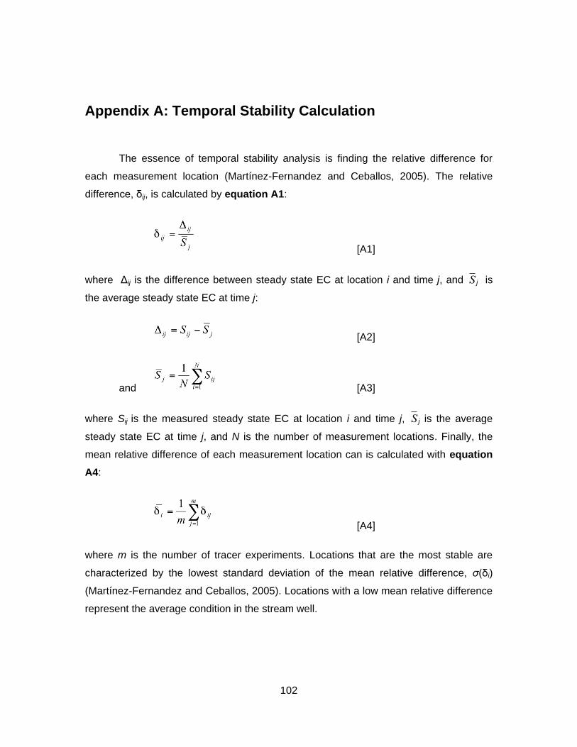
102

Appendix A: Temporal Stability Calculation

The essence of temporal stability analysis is finding the relative difference for

each measurement location (Martínez-Fernandez and Ceballos, 2005). The relative

difference, δij, is calculated by equation A1:

[A1]

where Δij is the difference between steady state EC at location i and time j, and

S j is

the average steady state EC at time j:

[A2]

and [A3]

where Sij is the measured steady state EC at location i and time j,

S j is the average

steady state EC at time j, and N is the number of measurement locations. Finally, the

mean relative difference of each measurement location can is calculated with equation

A4:

[A4]

where m is the number of tracer experiments. Locations that are the most stable are

characterized by the lowest standard deviation of the mean relative difference, σ(δi)

(Martínez-Fernandez and Ceballos, 2005). Locations with a low mean relative difference

represent the average condition in the stream well.

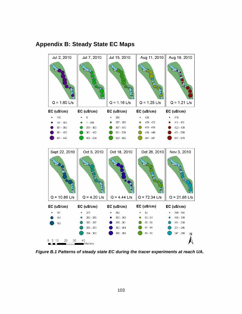
103

Appendix B: Steady State EC Maps

Figure B.1 Patterns of steady state EC during the tracer experiments at reach UA.

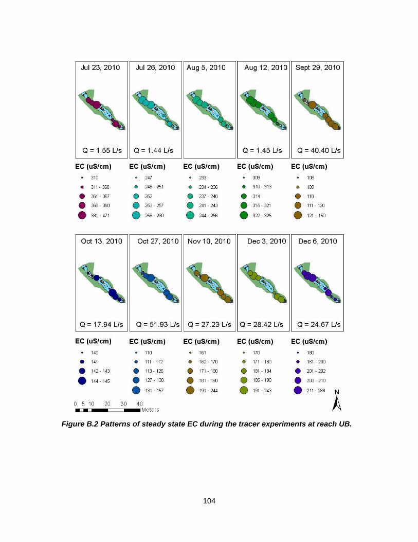
104

Figure B.2 Patterns of steady state EC during the tracer experiments at reach UB.

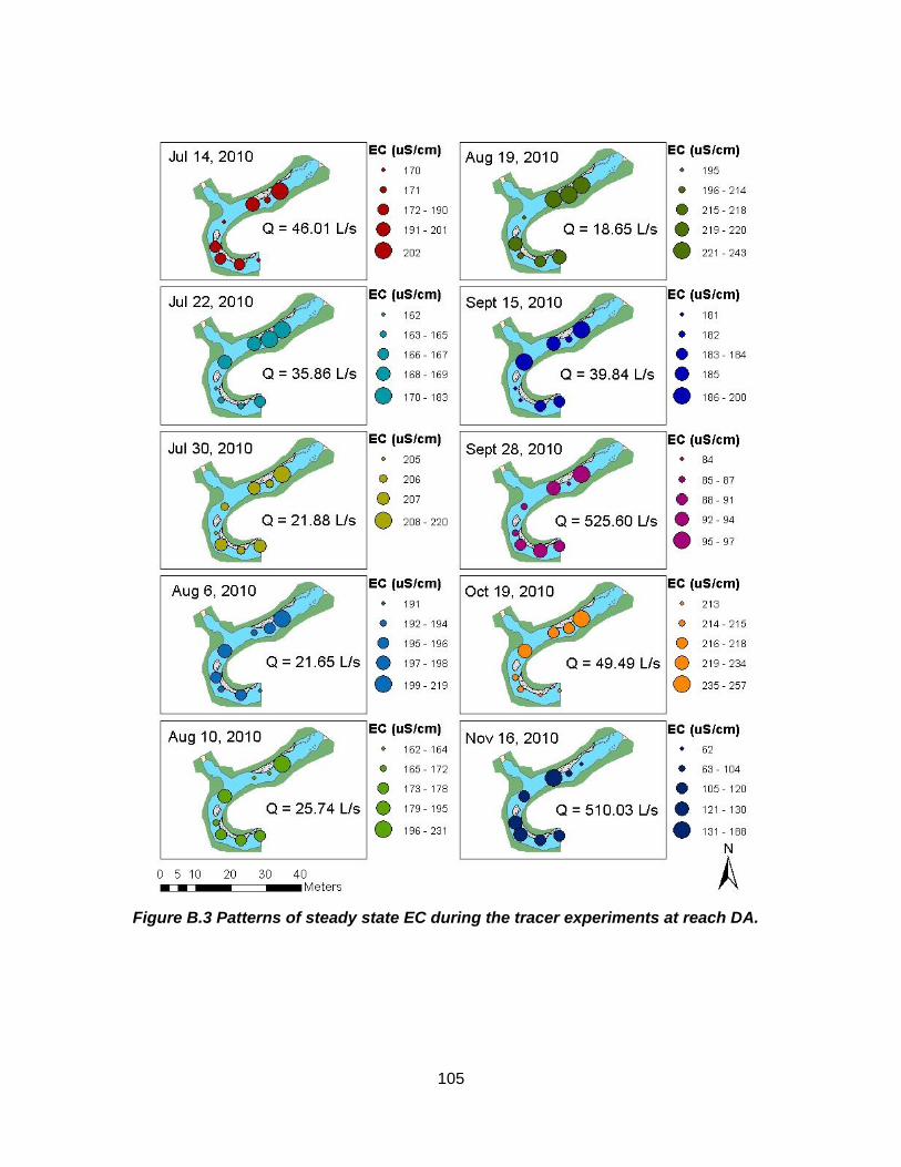
105

Figure B.3 Patterns of steady state EC during the tracer experiments at reach DA.

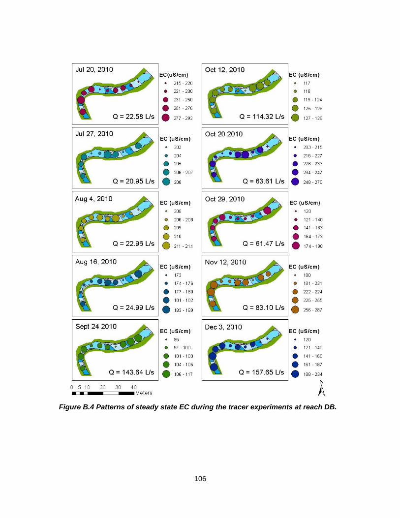
106

Figure B.4 Patterns of steady state EC during the tracer experiments at reach DB.

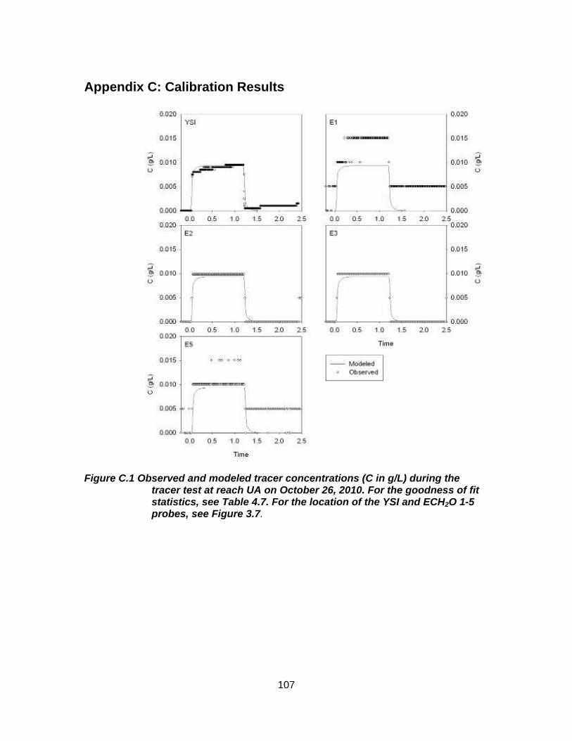
107

Appendix C: Calibration Results

Figure C.1 Observed and modeled tracer concentrations (C in g/L) during the tracer test at reach UA on October 26, 2010. For the goodness of fit statistics, see Table 4.7. For the location of the YSI and ECH2O 1-5 probes, see Figure 3.7.

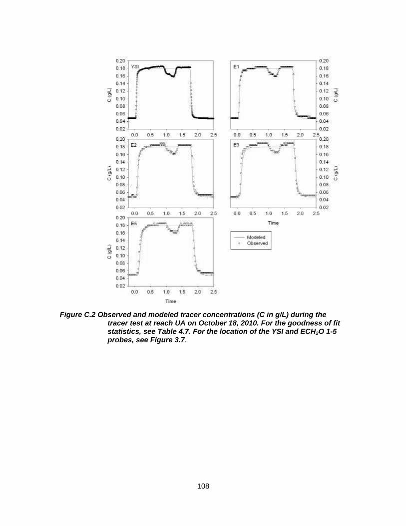
108

Figure C.2 Observed and modeled tracer concentrations (C in g/L) during the tracer test at reach UA on October 18, 2010. For the goodness of fit statistics, see Table 4.7. For the location of the YSI and ECH2O 1-5 probes, see Figure 3.7.

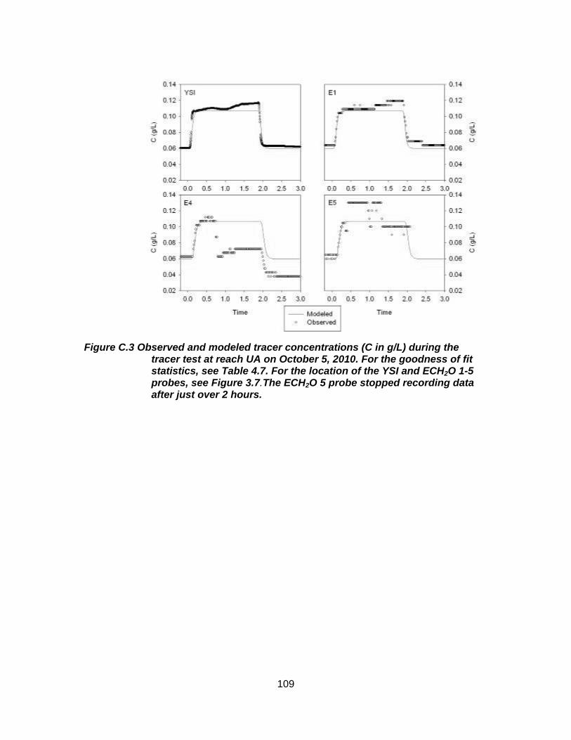
109

Figure C.3 Observed and modeled tracer concentrations (C in g/L) during the tracer test at reach UA on October 5, 2010. For the goodness of fit statistics, see Table 4.7. For the location of the YSI and ECH2O 1-5 probes, see Figure 3.7.The ECH2O 5 probe stopped recording data after just over 2 hours.

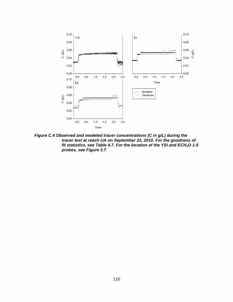
110

Figure C.4 Observed and modeled tracer concentrations (C in g/L) during the tracer test at reach UA on September 22, 2010. For the goodness of fit statistics, see Table 4.7. For the location of the YSI and ECH2O 1-5 probes, see Figure 3.7.

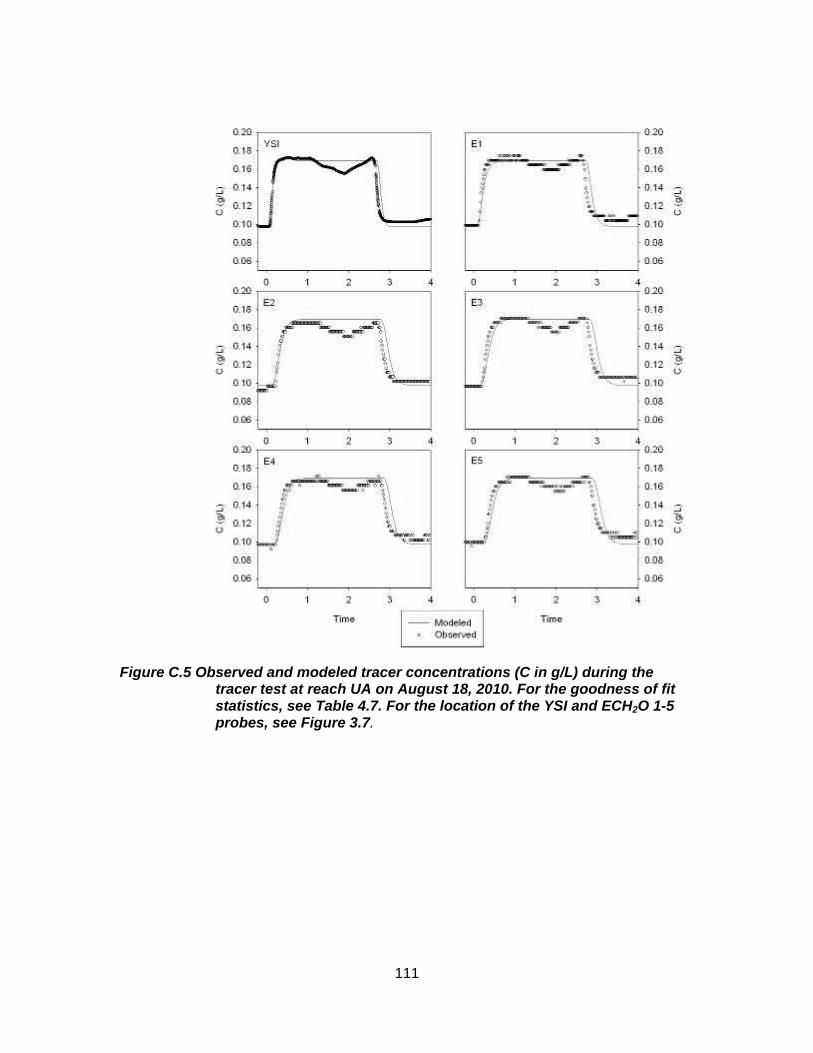
111

Figure C.5 Observed and modeled tracer concentrations (C in g/L) during the tracer test at reach UA on August 18, 2010. For the goodness of fit statistics, see Table 4.7. For the location of the YSI and ECH2O 1-5 probes, see Figure 3.7.

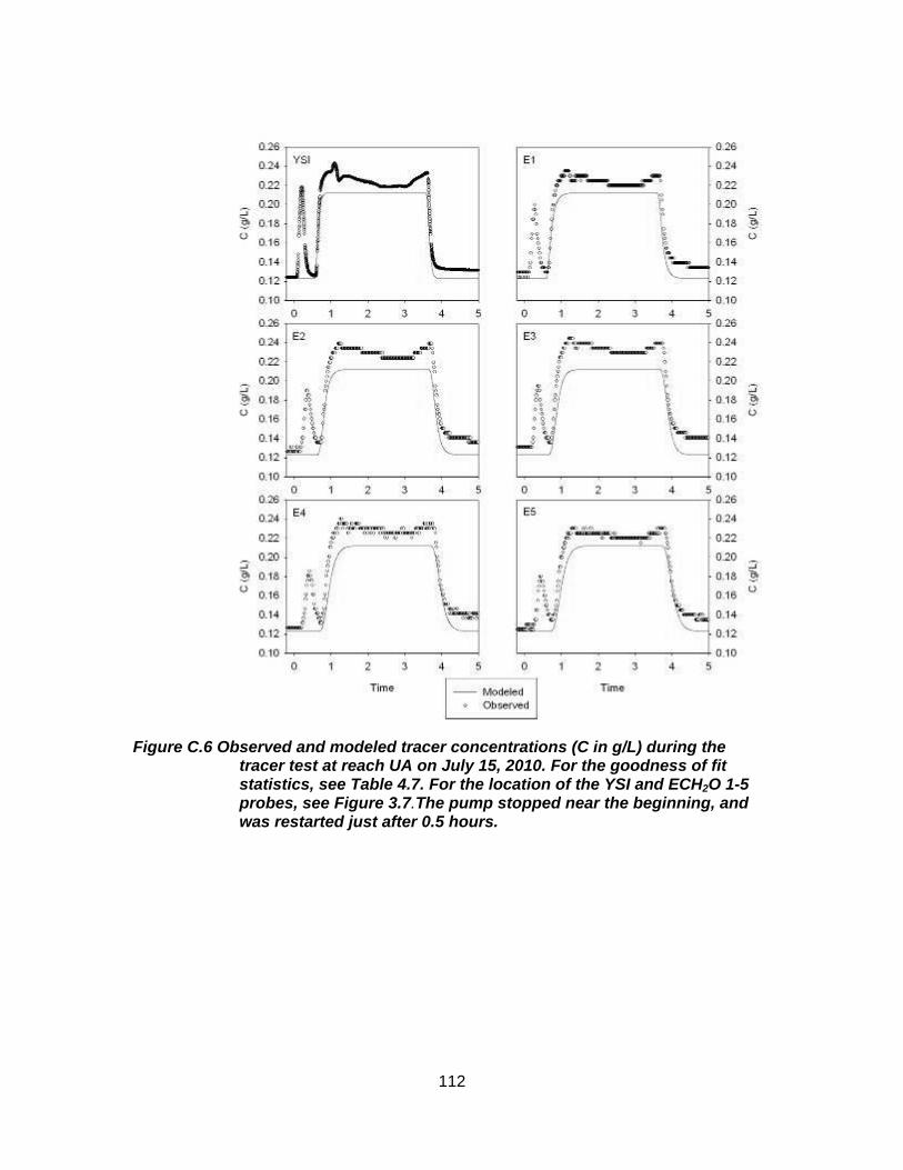
112

Figure C.6 Observed and modeled tracer concentrations (C in g/L) during the tracer test at reach UA on July 15, 2010. For the goodness of fit statistics, see Table 4.7. For the location of the YSI and ECH2O 1-5 probes, see Figure 3.7.The pump stopped near the beginning, and was restarted just after 0.5 hours.

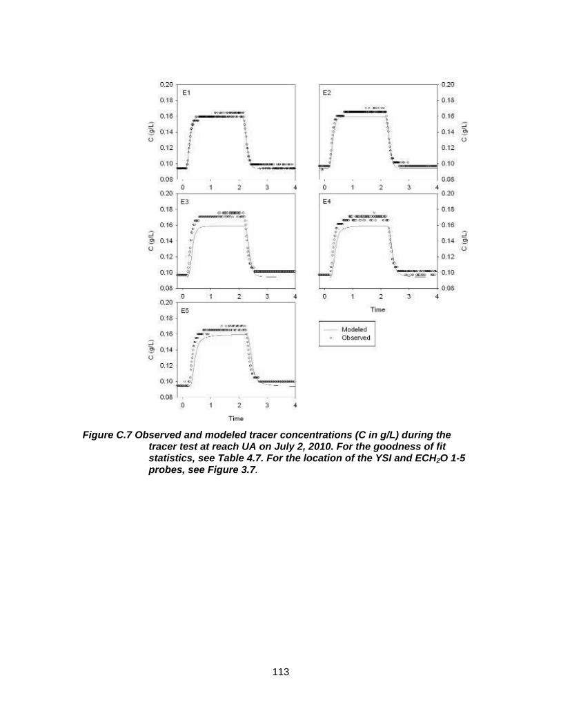
113

Figure C.7 Observed and modeled tracer concentrations (C in g/L) during the tracer test at reach UA on July 2, 2010. For the goodness of fit statistics, see Table 4.7. For the location of the YSI and ECH2O 1-5 probes, see Figure 3.7.

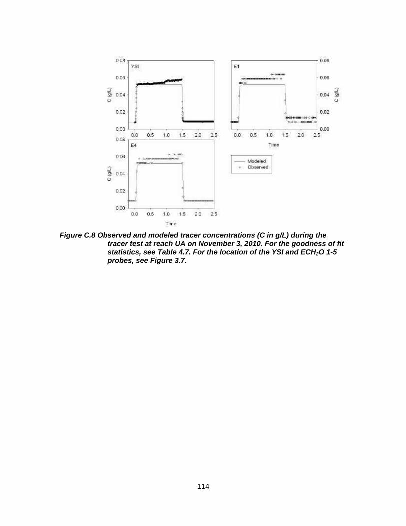
114

Figure C.8 Observed and modeled tracer concentrations (C in g/L) during the tracer test at reach UA on November 3, 2010. For the goodness of fit statistics, see Table 4.7. For the location of the YSI and ECH2O 1-5 probes, see Figure 3.7.

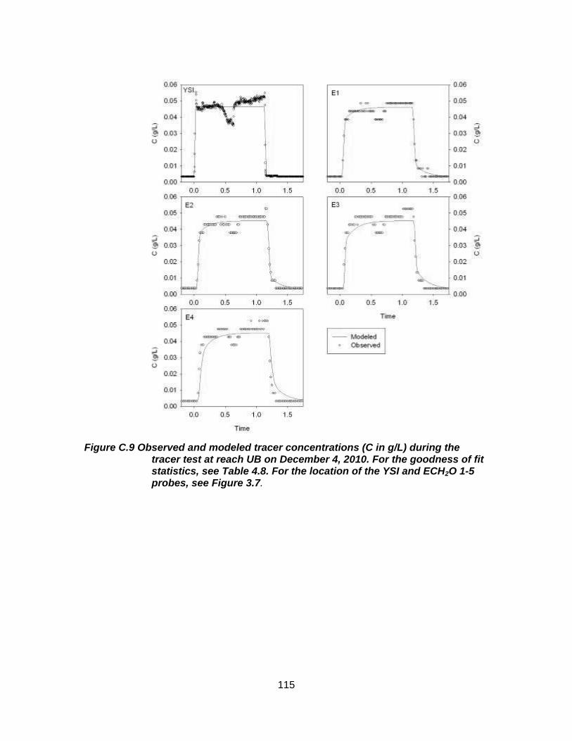
115

Figure C.9 Observed and modeled tracer concentrations (C in g/L) during the tracer test at reach UB on December 4, 2010. For the goodness of fit statistics, see Table 4.8. For the location of the YSI and ECH2O 1-5 probes, see Figure 3.7.

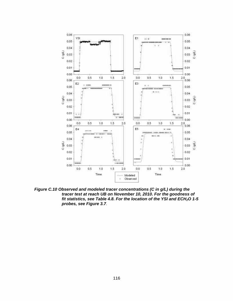
116

Figure C.10 Observed and modeled tracer concentrations (C in g/L) during the tracer test at reach UB on November 10, 2010. For the goodness of fit statistics, see Table 4.8. For the location of the YSI and ECH2O 1-5 probes, see Figure 3.7.

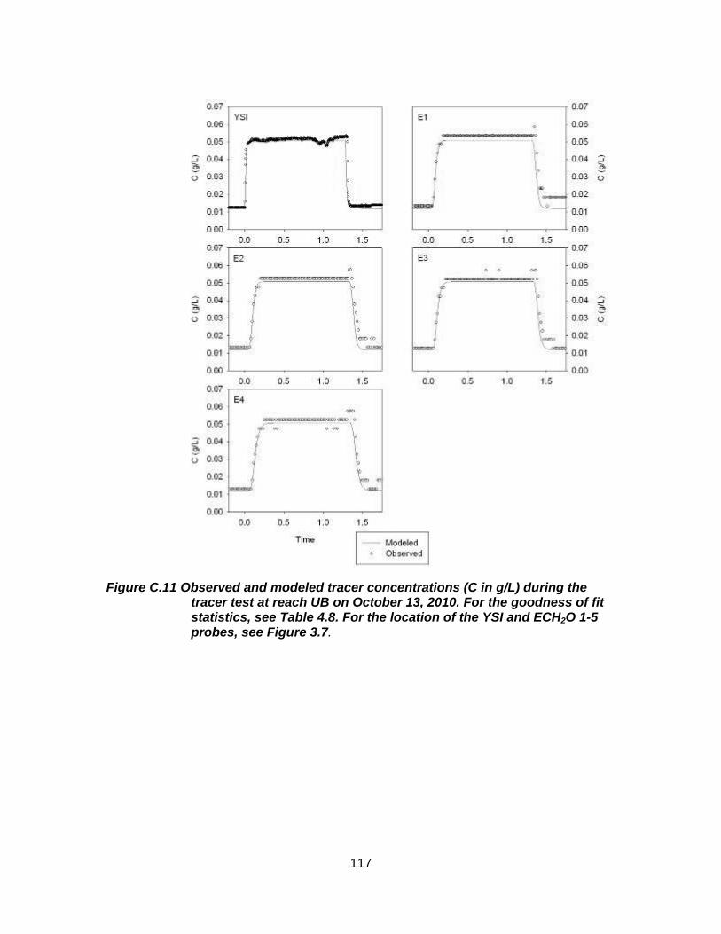
117

Figure C.11 Observed and modeled tracer concentrations (C in g/L) during the tracer test at reach UB on October 13, 2010. For the goodness of fit statistics, see Table 4.8. For the location of the YSI and ECH2O 1-5 probes, see Figure 3.7.

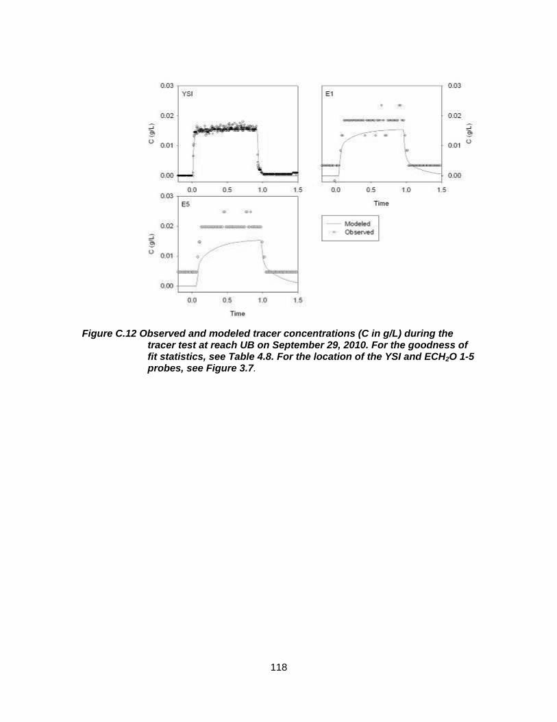
118

Figure C.12 Observed and modeled tracer concentrations (C in g/L) during the tracer test at reach UB on September 29, 2010. For the goodness of fit statistics, see Table 4.8. For the location of the YSI and ECH2O 1-5 probes, see Figure 3.7.

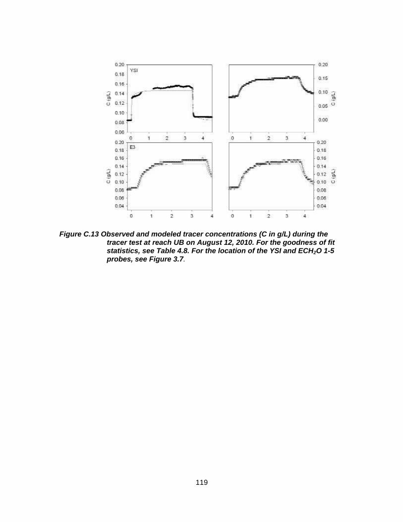
119

Figure C.13 Observed and modeled tracer concentrations (C in g/L) during the tracer test at reach UB on August 12, 2010. For the goodness of fit statistics, see Table 4.8. For the location of the YSI and ECH2O 1-5 probes, see Figure 3.7.

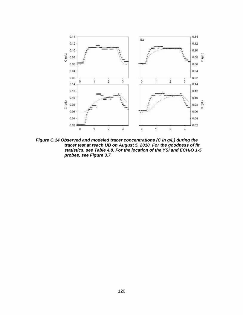
120

Figure C.14 Observed and modeled tracer concentrations (C in g/L) during the tracer test at reach UB on August 5, 2010. For the goodness of fit statistics, see Table 4.8. For the location of the YSI and ECH2O 1-5 probes, see Figure 3.7.

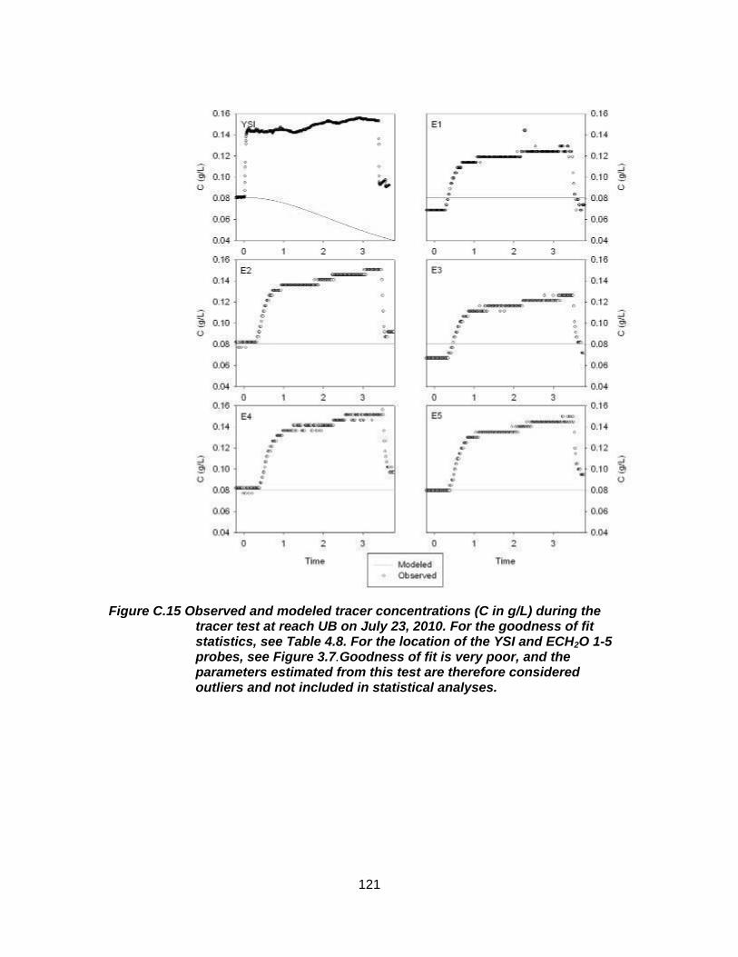
121

Figure C.15 Observed and modeled tracer concentrations (C in g/L) during the tracer test at reach UB on July 23, 2010. For the goodness of fit statistics, see Table 4.8. For the location of the YSI and ECH2O 1-5 probes, see Figure 3.7.Goodness of fit is very poor, and the parameters estimated from this test are therefore considered outliers and not included in statistical analyses.

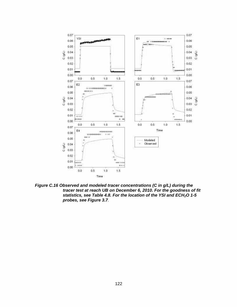
122

Figure C.16 Observed and modeled tracer concentrations (C in g/L) during the tracer test at reach UB on December 6, 2010. For the goodness of fit statistics, see Table 4.8. For the location of the YSI and ECH2O 1-5 probes, see Figure 3.7.

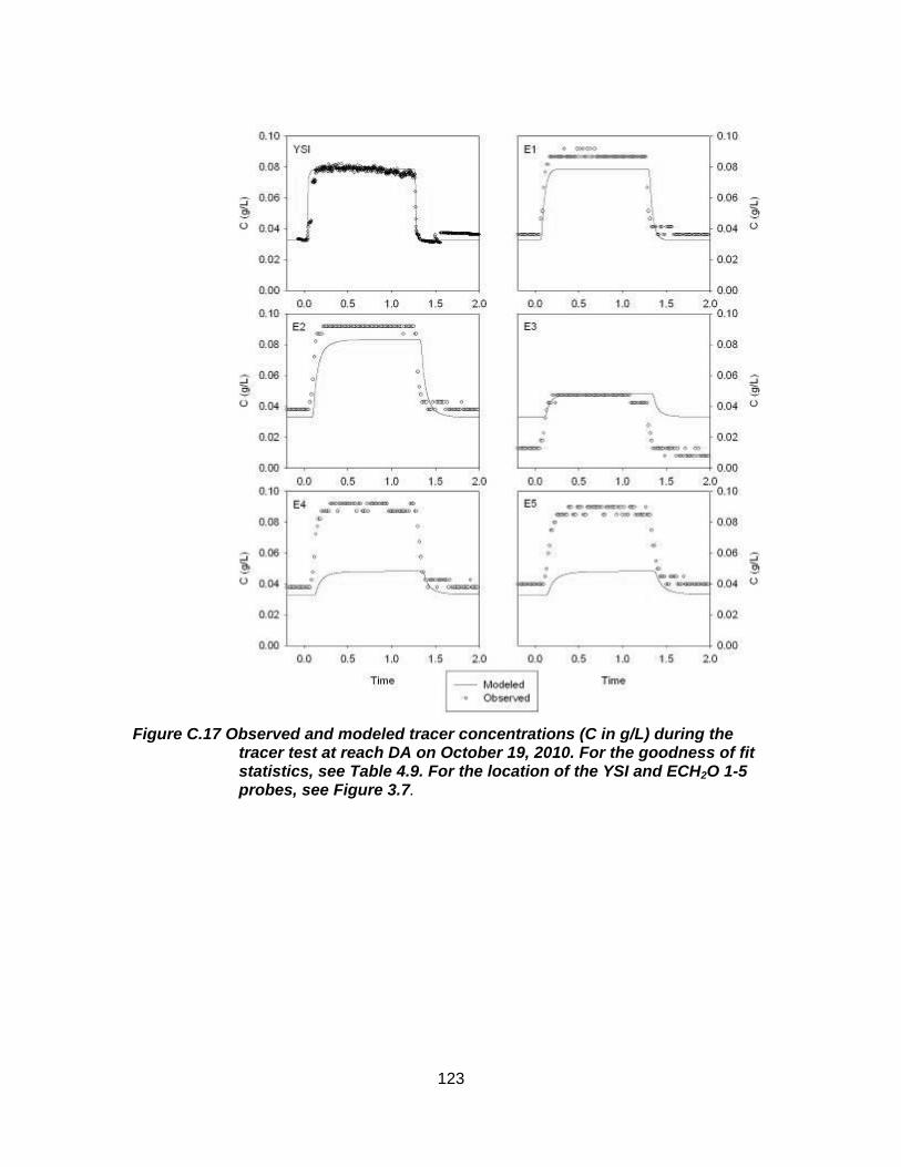
123

Figure C.17 Observed and modeled tracer concentrations (C in g/L) during the tracer test at reach DA on October 19, 2010. For the goodness of fit statistics, see Table 4.9. For the location of the YSI and ECH2O 1-5 probes, see Figure 3.7.

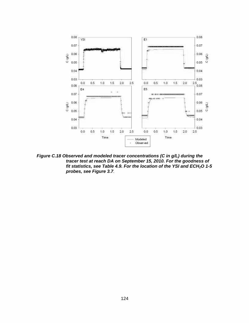
124

Figure C.18 Observed and modeled tracer concentrations (C in g/L) during the tracer test at reach DA on September 15, 2010. For the goodness of fit statistics, see Table 4.9. For the location of the YSI and ECH2O 1-5 probes, see Figure 3.7.

125

Figure C.19 Observed and modeled tracer concentrations (C in g/L) during the tracer test at reach DA on August 19, 2010. For the goodness of fit statistics, see Table 4.9. For the location of the YSI and ECH2O 1-5 probes, see Figure 3.7.

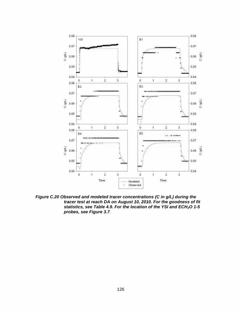
126

Figure C.20 Observed and modeled tracer concentrations (C in g/L) during the tracer test at reach DA on August 10, 2010. For the goodness of fit statistics, see Table 4.9. For the location of the YSI and ECH2O 1-5 probes, see Figure 3.7.

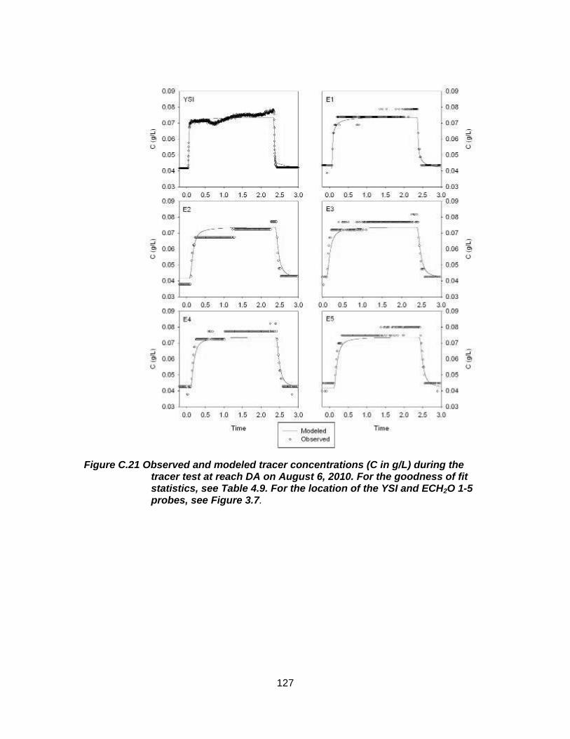
127

Figure C.21 Observed and modeled tracer concentrations (C in g/L) during the tracer test at reach DA on August 6, 2010. For the goodness of fit statistics, see Table 4.9. For the location of the YSI and ECH2O 1-5 probes, see Figure 3.7.

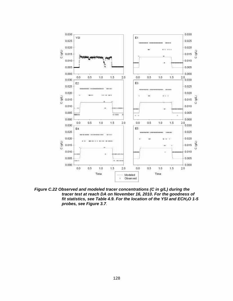
128

Figure C.22 Observed and modeled tracer concentrations (C in g/L) during the tracer test at reach DA on November 16, 2010. For the goodness of fit statistics, see Table 4.9. For the location of the YSI and ECH2O 1-5 probes, see Figure 3.7.

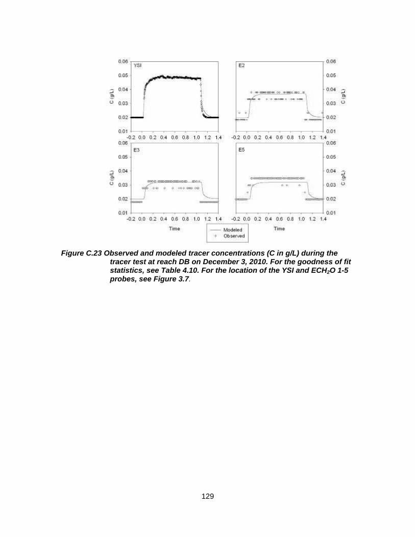
129

Figure C.23 Observed and modeled tracer concentrations (C in g/L) during the tracer test at reach DB on December 3, 2010. For the goodness of fit statistics, see Table 4.10. For the location of the YSI and ECH2O 1-5 probes, see Figure 3.7.

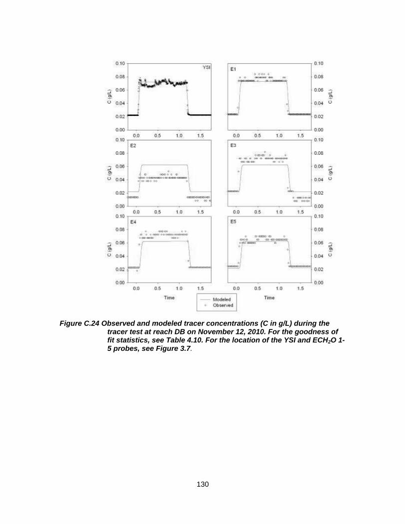
130

Figure C.24 Observed and modeled tracer concentrations (C in g/L) during the tracer test at reach DB on November 12, 2010. For the goodness of fit statistics, see Table 4.10. For the location of the YSI and ECH2O 1-5 probes, see Figure 3.7.

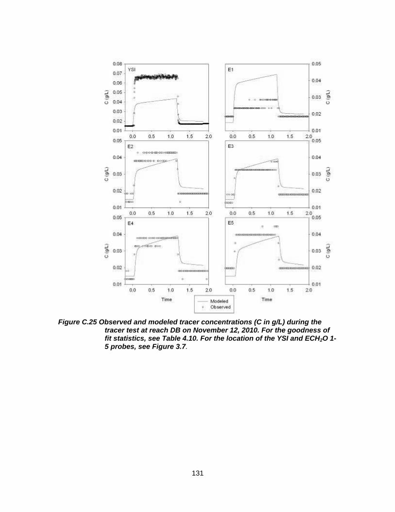
131

Figure C.25 Observed and modeled tracer concentrations (C in g/L) during the tracer test at reach DB on November 12, 2010. For the goodness of fit statistics, see Table 4.10. For the location of the YSI and ECH2O 1-5 probes, see Figure 3.7.

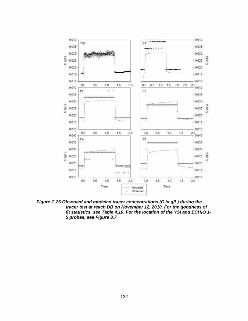
132

Figure C.26 Observed and modeled tracer concentrations (C in g/L) during the tracer test at reach DB on November 12, 2010. For the goodness of fit statistics, see Table 4.10. For the location of the YSI and ECH2O 1-5 probes, see Figure 3.7.

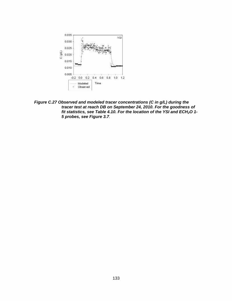
133

Figure C.27 Observed and modeled tracer concentrations (C in g/L) during the tracer test at reach DB on September 24, 2010. For the goodness of fit statistics, see Table 4.10. For the location of the YSI and ECH2O 1-5 probes, see Figure 3.7.

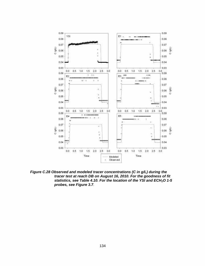
134

Figure C.28 Observed and modeled tracer concentrations (C in g/L) during the tracer test at reach DB on August 16, 2010. For the goodness of fit statistics, see Table 4.10. For the location of the YSI and ECH2O 1-5 probes, see Figure 3.7.

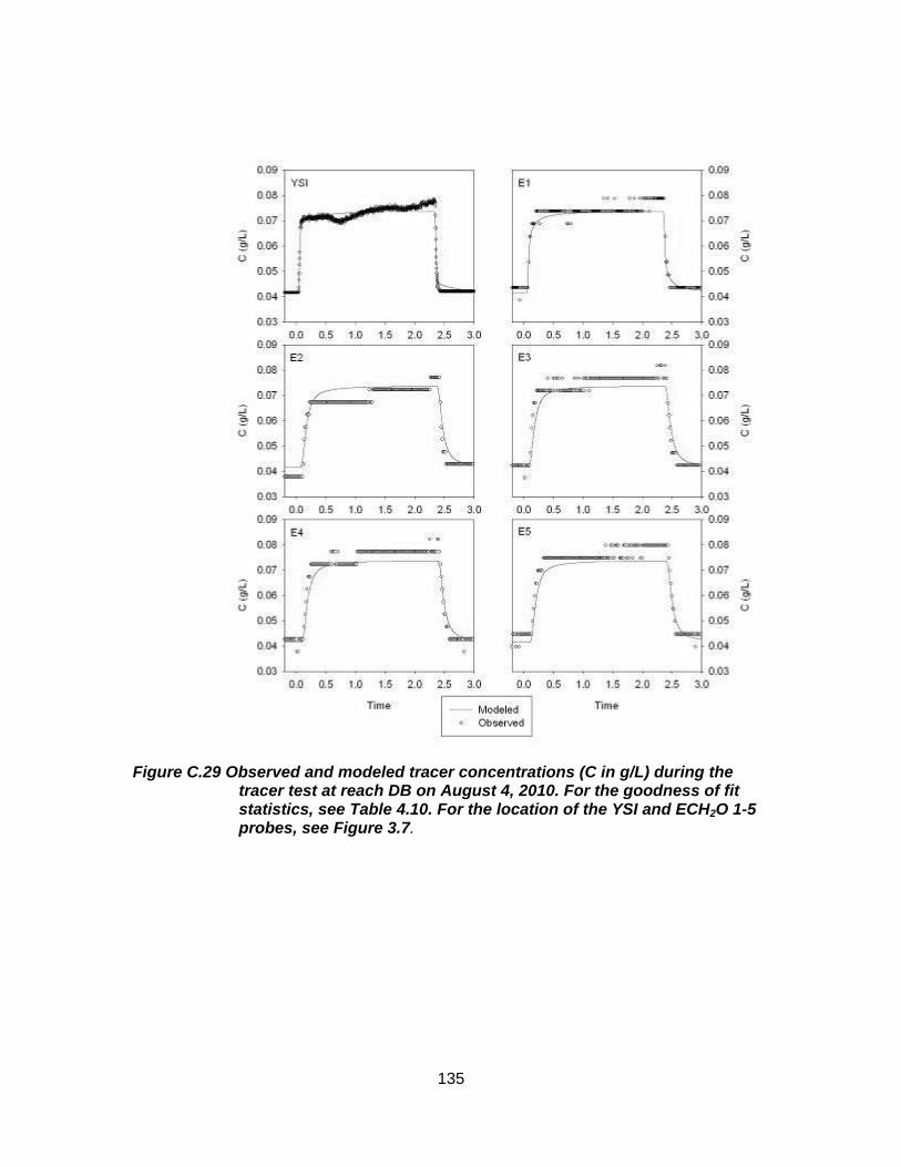
135

Figure C.29 Observed and modeled tracer concentrations (C in g/L) during the tracer test at reach DB on August 4, 2010. For the goodness of fit statistics, see Table 4.10. For the location of the YSI and ECH2O 1-5 probes, see Figure 3.7.

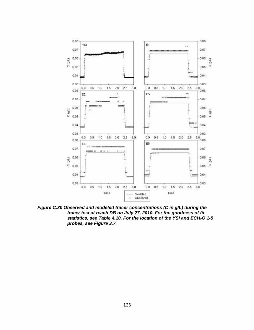
136

Figure C.30 Observed and modeled tracer concentrations (C in g/L) during the tracer test at reach DB on July 27, 2010. For the goodness of fit statistics, see Table 4.10. For the location of the YSI and ECH2O 1-5 probes, see Figure 3.7.

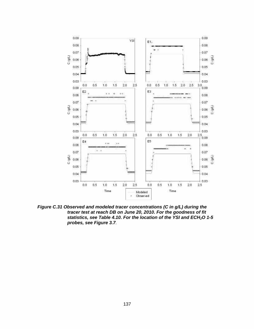
137

Figure C.31 Observed and modeled tracer concentrations (C in g/L) during the tracer test at reach DB on June 20, 2010. For the goodness of fit statistics, see Table 4.10. For the location of the YSI and ECH2O 1-5 probes, see Figure 3.7.

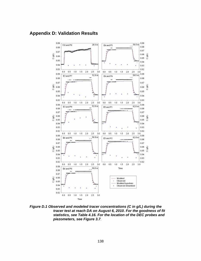
138

Appendix D: Validation Results

Figure D.1 Observed and modeled tracer concentrations (C in g/L) during the tracer test at reach DA on August 6, 2010. For the goodness of fit statistics, see Table 4.16. For the location of the DEC probes and piezometers, see Figure 3.7.

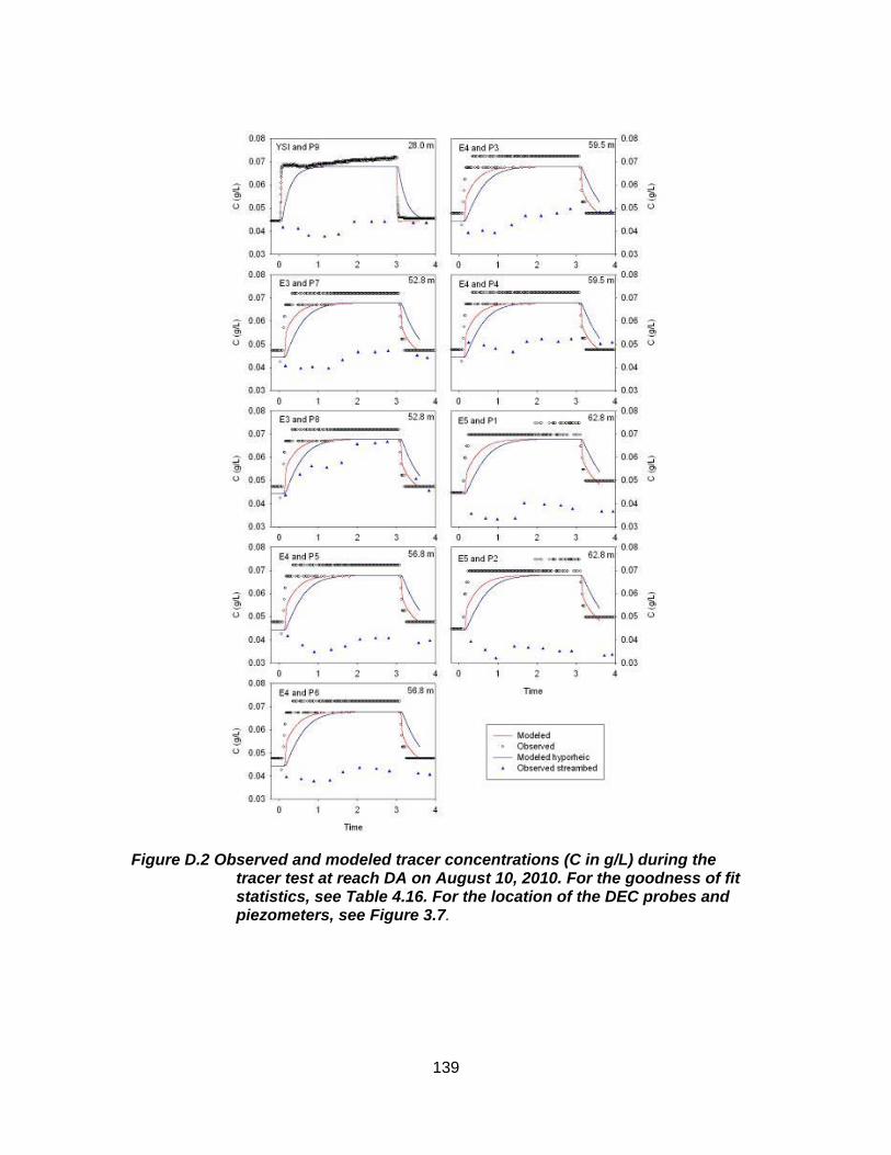
139

Figure D.2 Observed and modeled tracer concentrations (C in g/L) during the tracer test at reach DA on August 10, 2010. For the goodness of fit statistics, see Table 4.16. For the location of the DEC probes and piezometers, see Figure 3.7.

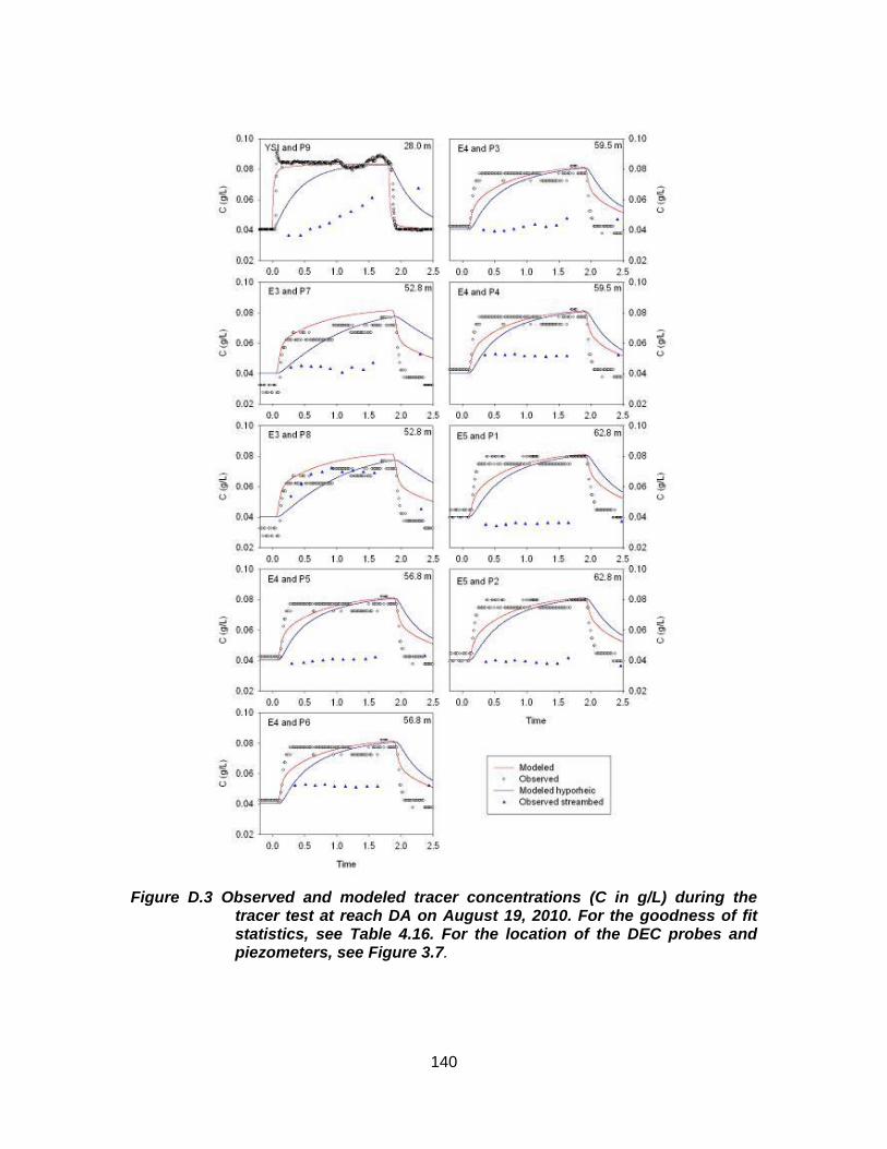
140

Figure D.3 Observed and modeled tracer concentrations (C in g/L) during the tracer test at reach DA on August 19, 2010. For the goodness of fit statistics, see Table 4.16. For the location of the DEC probes and piezometers, see Figure 3.7.

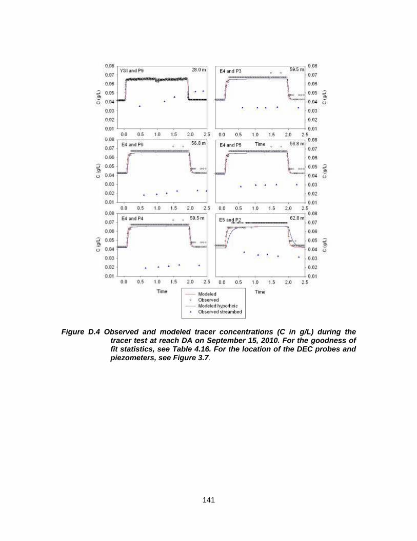
141

Figure D.4 Observed and modeled tracer concentrations (C in g/L) during the tracer test at reach DA on September 15, 2010. For the goodness of fit statistics, see Table 4.16. For the location of the DEC probes and piezometers, see Figure 3.7.

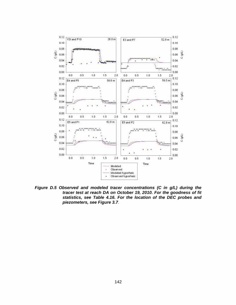
142

Figure D.5 Observed and modeled tracer concentrations (C in g/L) during the tracer test at reach DA on October 19, 2010. For the goodness of fit statistics, see Table 4.16. For the location of the DEC probes and piezometers, see Figure 3.7.

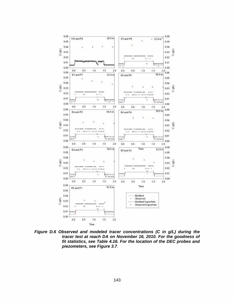
143

Figure D.6 Observed and modeled tracer concentrations (C in g/L) during the tracer test at reach DA on November 16, 2010. For the goodness of fit statistics, see Table 4.16. For the location of the DEC probes and piezometers, see Figure 3.7.

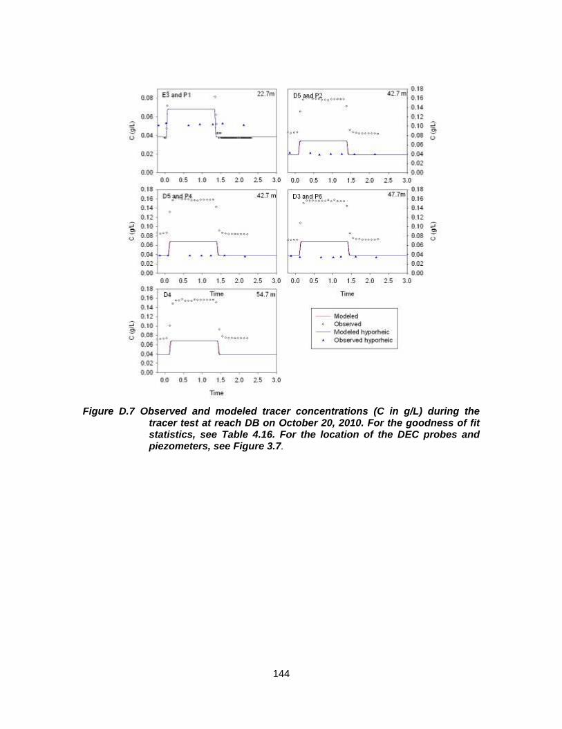
144

Figure D.7 Observed and modeled tracer concentrations (C in g/L) during the tracer test at reach DB on October 20, 2010. For the goodness of fit statistics, see Table 4.16. For the location of the DEC probes and piezometers, see Figure 3.7.

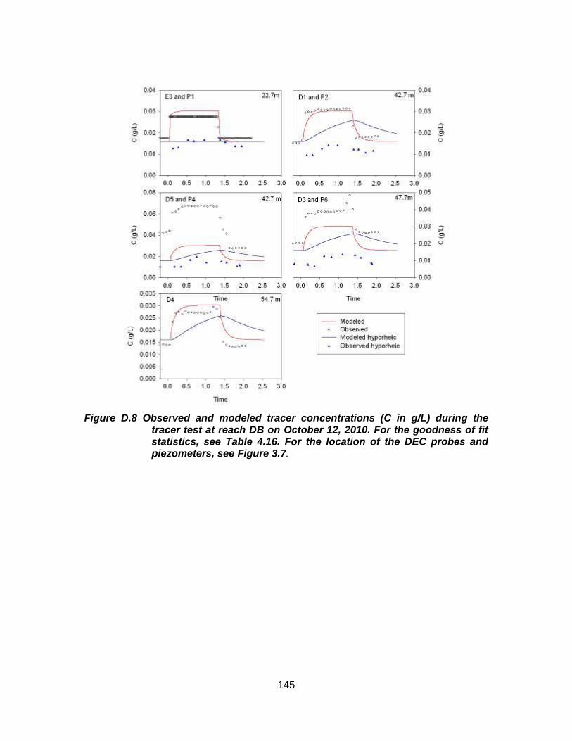
145

Figure D.8 Observed and modeled tracer concentrations (C in g/L) during the tracer test at reach DB on October 12, 2010. For the goodness of fit statistics, see Table 4.16. For the location of the DEC probes and piezometers, see Figure 3.7.

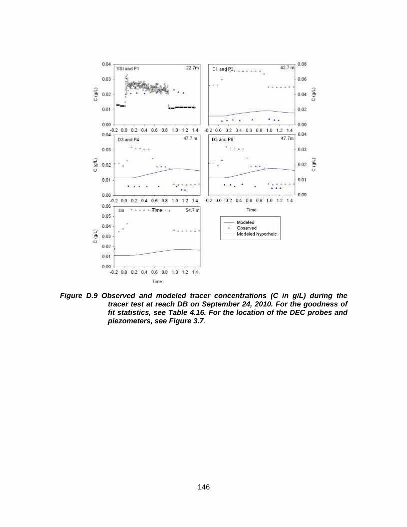
146

Figure D.9 Observed and modeled tracer concentrations (C in g/L) during the tracer test at reach DB on September 24, 2010. For the goodness of fit statistics, see Table 4.16. For the location of the DEC probes and piezometers, see Figure 3.7.

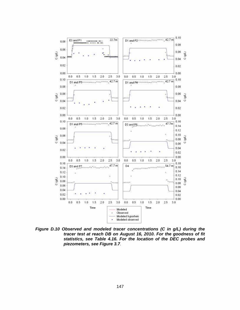
147

Figure D.10 Observed and modeled tracer concentrations (C in g/L) during the tracer test at reach DB on August 16, 2010. For the goodness of fit statistics, see Table 4.16. For the location of the DEC probes and piezometers, see Figure 3.7.

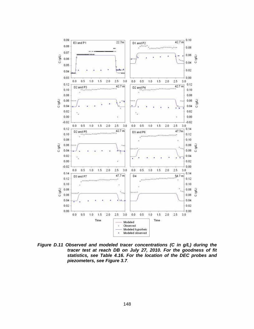
148

Figure D.11 Observed and modeled tracer concentrations (C in g/L) during the tracer test at reach DB on July 27, 2010. For the goodness of fit statistics, see Table 4.16. For the location of the DEC probes and piezometers, see Figure 3.7.

149

Figure D.12 Observed and modeled tracer concentrations (C in g/L) during the tracer test at reach DB on July 20, 2010. For the goodness of fit statistics, see Table 4.16. For the location of the DEC probes and piezometers, see Figure 3.7.

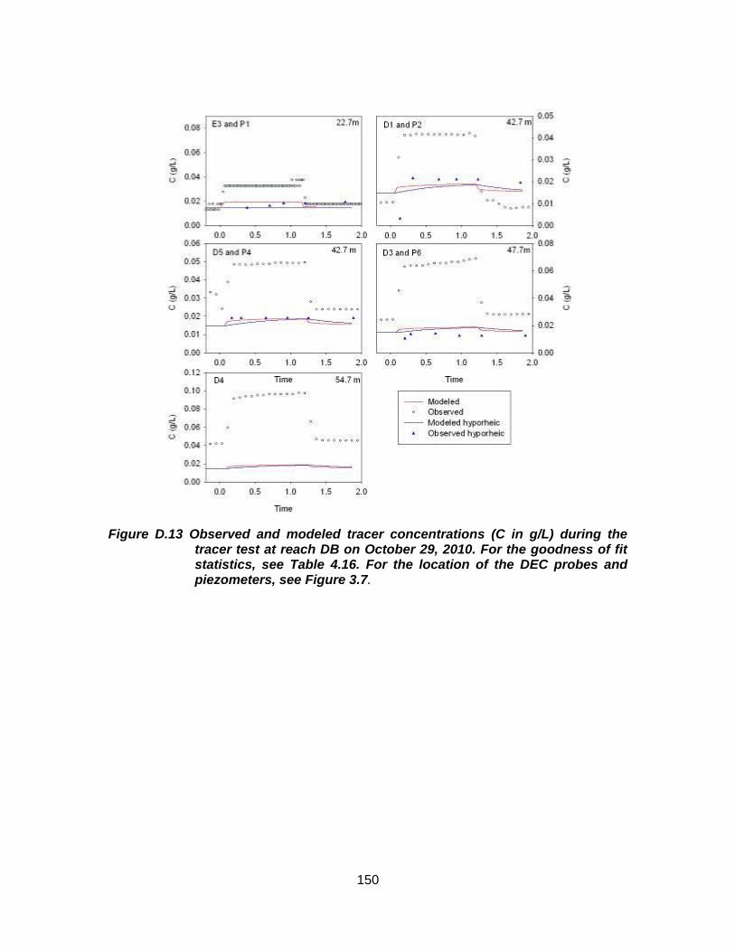
150

Figure D.13 Observed and modeled tracer concentrations (C in g/L) during the tracer test at reach DB on October 29, 2010. For the goodness of fit statistics, see Table 4.16. For the location of the DEC probes and piezometers, see Figure 3.7.

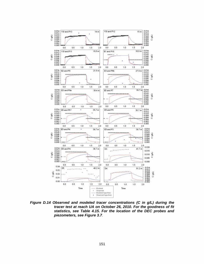
151

Figure D.14 Observed and modeled tracer concentrations (C in g/L) during the tracer test at reach UA on October 26, 2010. For the goodness of fit statistics, see Table 4.15. For the location of the DEC probes and piezometers, see Figure 3.7.

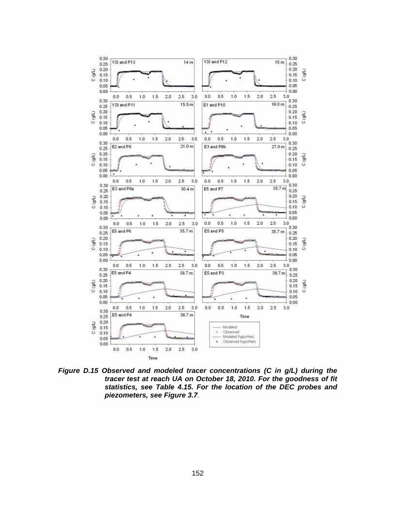
152

Figure D.15 Observed and modeled tracer concentrations (C in g/L) during the tracer test at reach UA on October 18, 2010. For the goodness of fit statistics, see Table 4.15. For the location of the DEC probes and piezometers, see Figure 3.7.

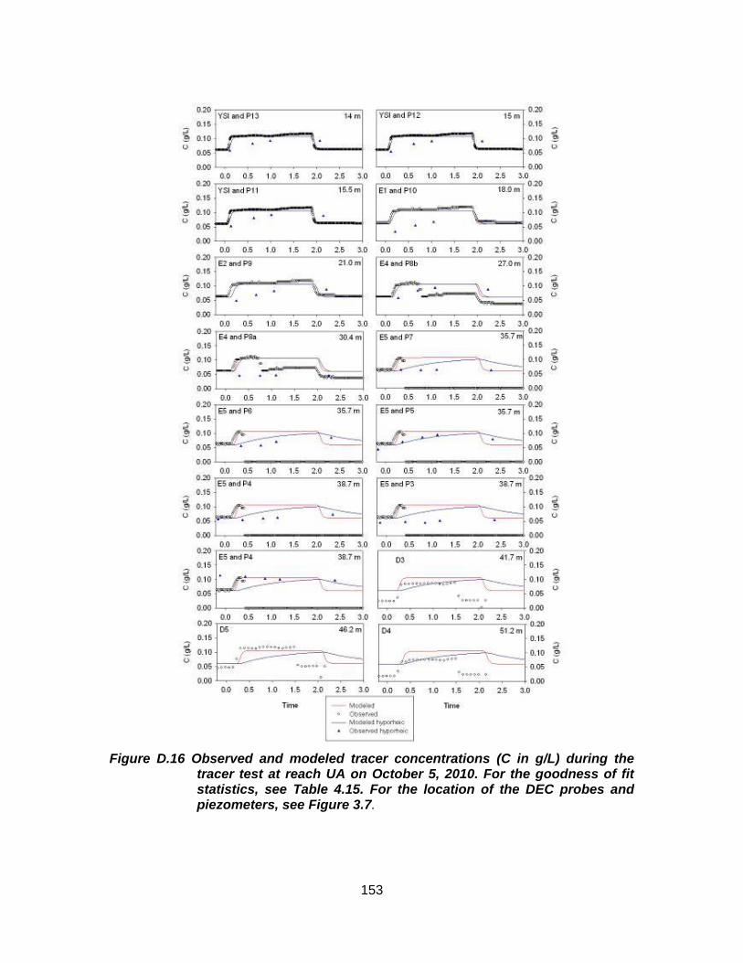
153

Figure D.16 Observed and modeled tracer concentrations (C in g/L) during the tracer test at reach UA on October 5, 2010. For the goodness of fit statistics, see Table 4.15. For the location of the DEC probes and piezometers, see Figure 3.7.

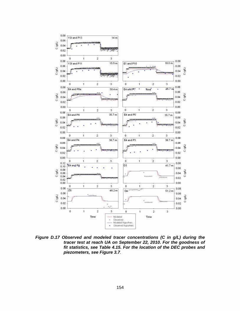
154

Figure D.17 Observed and modeled tracer concentrations (C in g/L) during the tracer test at reach UA on September 22, 2010. For the goodness of fit statistics, see Table 4.15. For the location of the DEC probes and piezometers, see Figure 3.7.

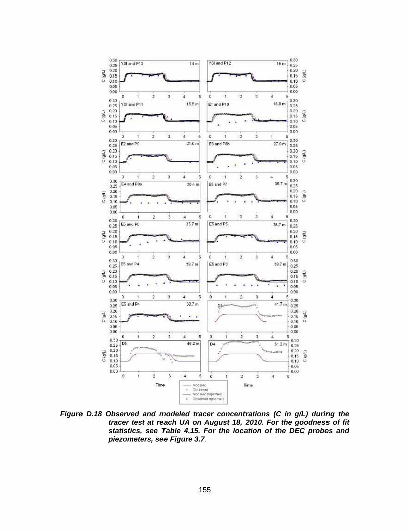
155

Figure D.18 Observed and modeled tracer concentrations (C in g/L) during the tracer test at reach UA on August 18, 2010. For the goodness of fit statistics, see Table 4.15. For the location of the DEC probes and piezometers, see Figure 3.7.

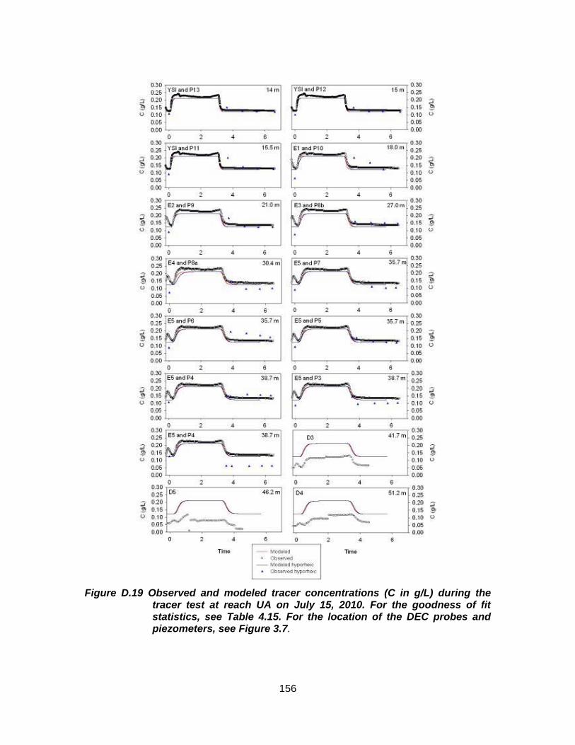
156

Figure D.19 Observed and modeled tracer concentrations (C in g/L) during the tracer test at reach UA on July 15, 2010. For the goodness of fit statistics, see Table 4.15. For the location of the DEC probes and piezometers, see Figure 3.7.

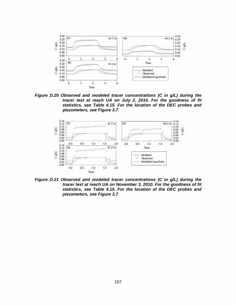
157

Figure D.20 Observed and modeled tracer concentrations (C in g/L) during the tracer test at reach UA on July 2, 2010. For the goodness of fit statistics, see Table 4.15. For the location of the DEC probes and piezometers, see Figure 3.7.

Figure D.21 Observed and modeled tracer concentrations (C in g/L) during the tracer test at reach UA on November 3, 2010. For the goodness of fit statistics, see Table 4.15. For the location of the DEC probes and piezometers, see Figure 3.7.

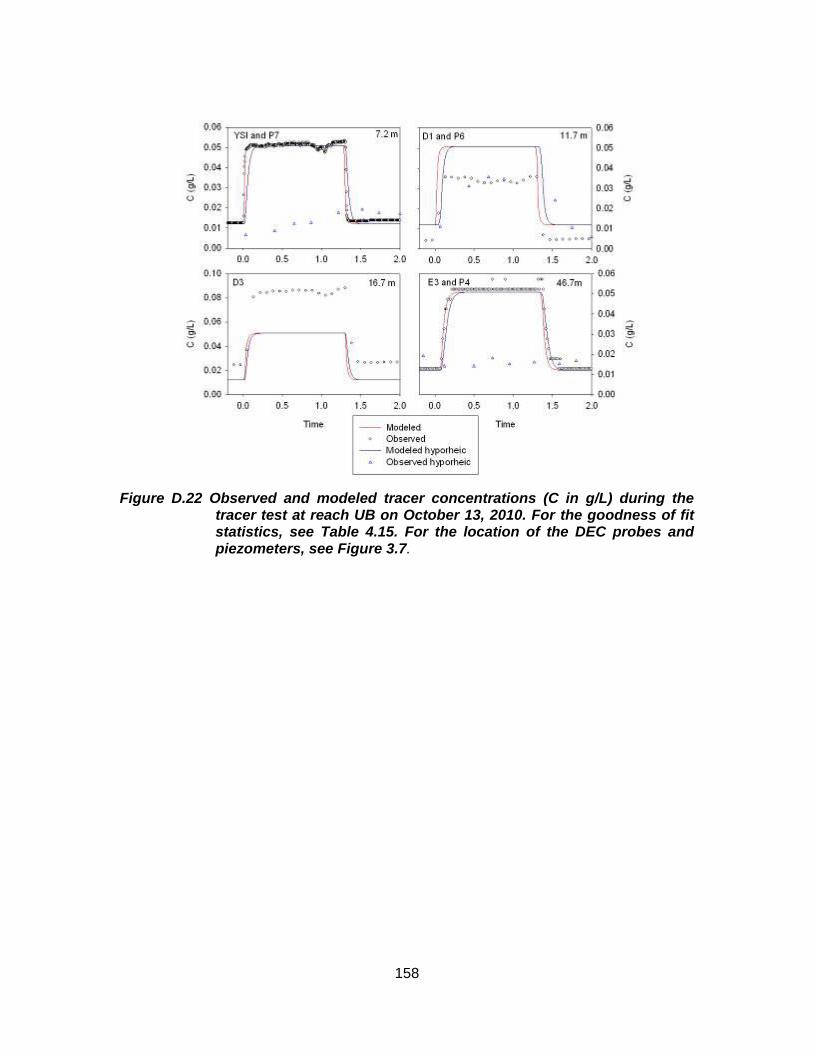
158

Figure D.22 Observed and modeled tracer concentrations (C in g/L) during the tracer test at reach UB on October 13, 2010. For the goodness of fit statistics, see Table 4.15. For the location of the DEC probes and piezometers, see Figure 3.7.

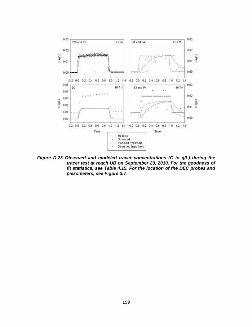
159

Figure D.23 Observed and modeled tracer concentrations (C in g/L) during the tracer test at reach UB on September 29, 2010. For the goodness of fit statistics, see Table 4.15. For the location of the DEC probes and piezometers, see Figure 3.7.

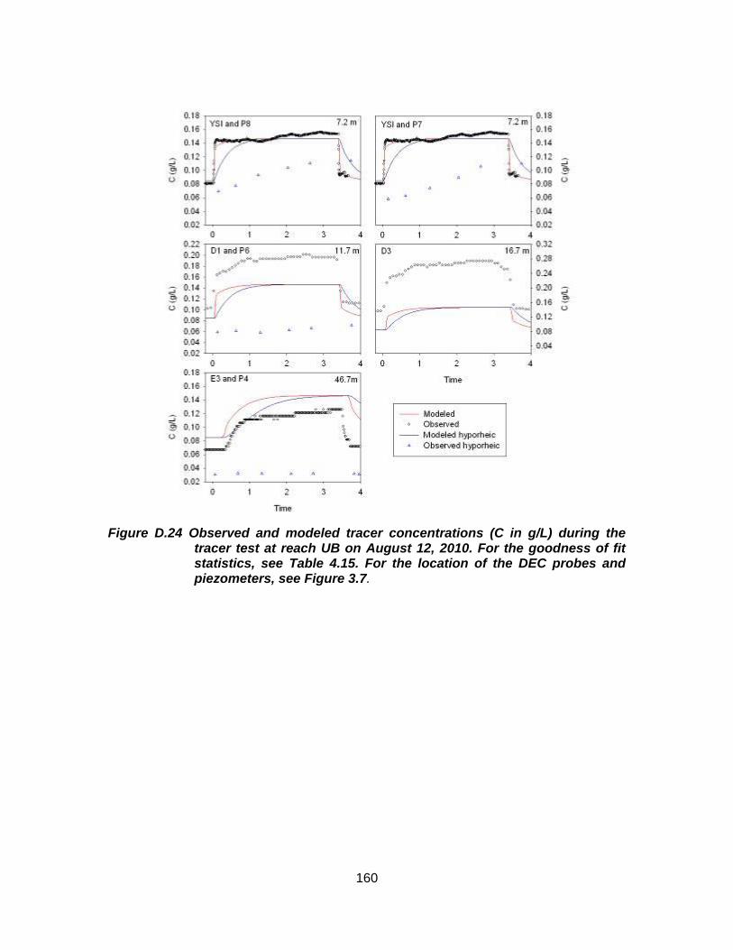
160

Figure D.24 Observed and modeled tracer concentrations (C in g/L) during the tracer test at reach UB on August 12, 2010. For the goodness of fit statistics, see Table 4.15. For the location of the DEC probes and piezometers, see Figure 3.7.

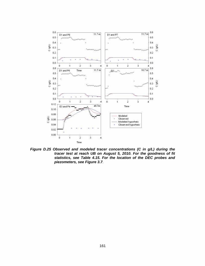
161

Figure D.25 Observed and modeled tracer concentrations (C in g/L) during the tracer test at reach UB on August 5, 2010. For the goodness of fit statistics, see Table 4.15. For the location of the DEC probes and piezometers, see Figure 3.7.

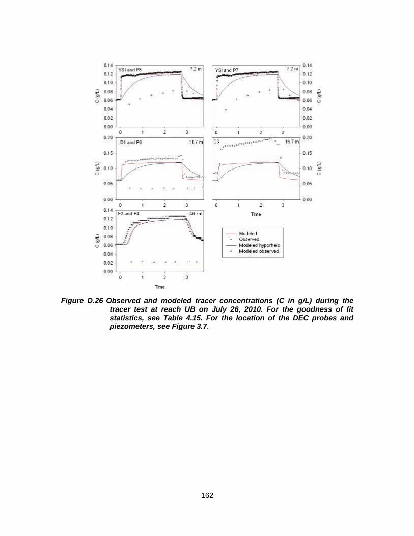
162

Figure D.26 Observed and modeled tracer concentrations (C in g/L) during the tracer test at reach UB on July 26, 2010. For the goodness of fit statistics, see Table 4.15. For the location of the DEC probes and piezometers, see Figure 3.7.

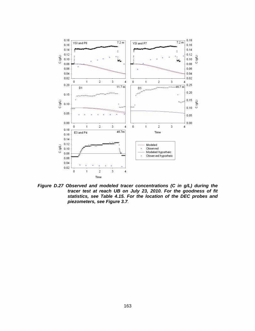
163

Figure D.27 Observed and modeled tracer concentrations (C in g/L) during the tracer test at reach UB on July 23, 2010. For the goodness of fit statistics, see Table 4.15. For the location of the DEC probes and piezometers, see Figure 3.7.

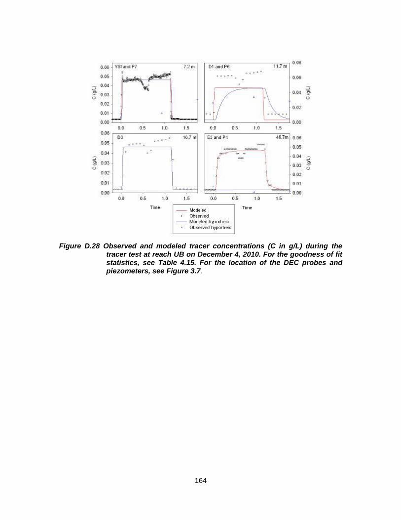
164

Figure D.28 Observed and modeled tracer concentrations (C in g/L) during the tracer test at reach UB on December 4, 2010. For the goodness of fit statistics, see Table 4.15. For the location of the DEC probes and piezometers, see Figure 3.7.