INFLATION IN

NEPAL

Nepal Rastra Bank, Research Department

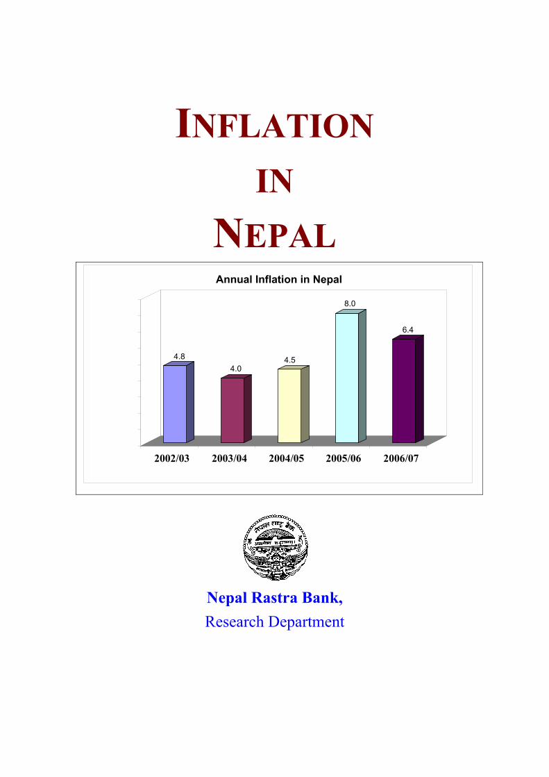
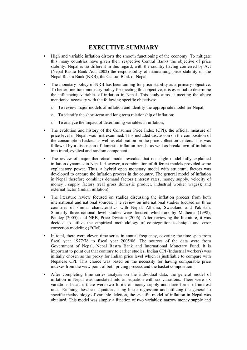
4.84.0

4.5

8.0

6.4

2002/03 2003/04 2004/05 2005/06 2006/07

Annual Inflation in Nepal

© 2007 Nepal Rastra Bank

Central Office

Baluwatar, Kathmandu

Nepal

Website: http://www.nrb.org.np

All rights reserved.

Cover design: Mr. Sundar Shrestha

Printed by: Nepal Rastra Bank.

TABLE OF CONTENTS Description Page No.

Foreword

Acknowledgements

Executive Summary

List of Tables, Boxes and Figures

Acronyms

1 Introduction 1

2 Historical Overview of Inflation 5

3 Theories of Inflation 11

4 Literature Review 17

5 Empirical Exercises 23

6 Analysis 31

7 Conclusion and Recommendations 36

References 38

Annexes 41

FOREWORD Excess inflation detracts from sustainable economic growth and development. The detrimental effect of high inflation comes largely through the channel of increased uncertainty, which has been shown empirically in many studies. Because of this effect, many monetary authorities have been given the responsibility of keeping inflation at a level consistent with that needed for smooth growth of the economy.

Nepal is also aware of the importance of having price stability for attaining sustained domestic economic growth. In this reference, the grave responsibility for maintaining price stability has been conferred upon the Nepal Rastra Bank (NRB) by the Nepal Rastra Bank Act, 2002. For the Bank to adequately discharge this responsibility, it is important to identify and determine the factors that influence inflation in the country, so that it can adequately manage and control and also accurately forecast the domestic inflation situation. To address the above-mentioned necessity, the Bank's Research Department has undergone an intensive research activity in this regard. I feel that the output of this important study entitled “Inflation in Nepal” well reflects the awareness by the NRB of the critical responsibility for maintaining domestic price stability, and is a seminal publication for understanding the dynamics of inflation in the country.

I would also mention that this publication is the product of coordinated effort from two Divisions of Research Department: the lead division being the Price Division and the supporting division being the Economic Analysis Division. I feel that the joint effort of both divisions, the first a line division and the later an analytical division, have led to positive synergy with the ensuing result being much more than the sum of the individual divisional contributions. This sort of joint activity, in my view, has worked very well and thus augers for many other such coordinated research activities in the future. In other words, this type of research activity and high-quality output from NRB will not be the exception but the rule, as the coming days will show.

This study had tremendous implication for policy issues in monetary and fiscal management in Nepal. While NRB is seeking the avenues for maintaining domestic price stability, the empirical results of the study are also applicable in foreign exchange management and analyzing the possibility of capital account convertibility. This study will also provide basis for inflation targeting, “as an anchor for monetary policy” of NRB.

I would like to acknowledge all the persons those contributed in shaping this study. I would like to thank for valuable comments by Prof. Dr. Gunanidhi Sharma and Dr. Shankar Sharma.

Finally, I would appreciate the endeavors of Research Department particularly joint efforts of Price Division and Economic Analysis Division for shaping the study in present form.

By ending I would express my strong conviction that this seminal publication will be very beneficial and serve as both a reference paradigm to those interested on the topic of inflation in Nepal and basis for further research, in this regard.

Krishna Bahadur Manandhar Acting Governor

ACKNOWLEDGEMENTS Achieving a low and stable inflation is the prime goal of monetary policy. To this end, the Nepal Rastra Bank as the monetary authority of the country has been committed for long. However, the dynamics of price and inflation in Nepal is somewhat complex mainly because of the large trade dependence with India, along with sharing the open border. Also the level of financial development is still at the nascent stage in Nepal. In this context, the present study attempts to delineate the possible factors determining inflation in Nepal.

Though a few studies in the past have tried to capture the factors contributing to the Nepalese inflation, they were on individual basis. But, the present study is an institutional effort to that direction. This study has also tried to apply some of the selected econometric models such as cointegration test, error correction model, and ordinary least square regression. The study develops a hybrid model of inflation for Nepal consisting of both monetary and structural factors. The study further reiterates that the role of Indian inflation has direct impact on the Nepalese inflation in both short and long term.

At this moment, I would like to acknowledge the efforts put forth by a number of people who contributed to this endeavor. I am thankful to Acting Governor Krishna Bahadur Manandhar for chairing the interaction program, and Professor Gunanidhi Sharma, and Dr. Shanker Sharma for critically reviewing the paper. I appreciate the guidance of Directors Mr. Trilochan Pangeni and Mrs. Rameswori Pant, and comments from Director Mr. Nara Bahadur Thapa. Likewise, Deputy Director Mr. Gopal Prasad Bhatta, and Assistant Directors; Mr. Dilaram Subedi and Dr. Khemraj Bhetuwal, all from Price Division; and Deputy Director Dr. Nephil Matangi Maskay, and Assistant Director Mr. Satyendra Raj Subedi, both from the Economic Analysis Division deserve special mentioning for their untiring and sincere efforts. The hard work of Mr. BBsen Maharjan in formatting and processing, and of Mr.Sundar Shrestha for cover designing is highly appreciated.

Ram Prasad Adhikary

Executive Director

EXECUTIVE SUMMARY • High and variable inflation distorts the smooth functioning of the economy. To mitigate

this many countries have given their respective Central Banks the objective of price stability. Nepal is no different in this regard, with the country having conferred by Act (Nepal Rastra Bank Act, 2002) the responsibility of maintaining price stability on the Nepal Rastra Bank (NRB), the Central Bank of Nepal.

• The monetary policy of NRB has been aiming for price stability as a primary objective. To better fine-tune monetary policy for meeting this objective, it is essential to determine the influencing variables of inflation in Nepal. This study aims at meeting the above mentioned necessity with the following specific objectives:

o To review major models of inflation and identify the appropriate model for Nepal;

o To identify the short-term and long term relationship of inflation;

o To analyze the impact of determining variables in inflation;

• The evolution and history of the Consumer Price Index (CPI), the official measure of price level in Nepal, was first examined. This included discussion on the composition of the consumption baskets as well as elaboration on the price collection centers. This was followed by a discussion of domestic inflation trends, as well as breakdown of inflation into trend, cyclical and random component.

• The review of major theoretical model revealed that no single model fully explained inflation dynamics in Nepal. However, a combination of different models provided some explanatory power. Thus, a hybrid open monetary model with structural factors was developed to capture the inflation process in the country. The general model of inflation in Nepal therefore combines demand factors (interest rates, money supply, velocity of money); supply factors (real gross domestic product, industrial worker wages); and external factor (Indian inflation).

• The literature review focused on studies discussing the inflation process from both international and national sources. The review on international studies focused on three countries of similar characteristics with Nepal: Albania, Swaziland and Pakistan. Similarly three national level studies were focused which are by Mathema (1998); Pandey (2005); and NRB, Price Division (2006). After reviewing the literature, it was decided to utilize the empirical methodology of cointegration technique and error correction modeling (ECM).

• In total, there were eleven time series in annual frequency, covering the time span from fiscal year 1977/78 to fiscal year 2005/06. The sources of the data were from Government of Nepal, Nepal Rastra Bank and International Monetary Fund. It is important to point out that contrary to earlier studies, Indian CPI (Industrial workers) was initially chosen as the proxy for Indian price level which is justifiable to compare with Nepalese CPI. This choice was based on the necessity for having comparable price indexes from the view point of both pricing process and the basket composition.

• After completing time series analysis on the individual data, the general model of inflation in Nepal was translated into an equation with six variations. There were six variations because there were two forms of money supply and three forms of interest rates. Running these six equations using linear regression and utilizing the general to specific methodology of variable deletion, the specific model of inflation in Nepal was obtained. This model was simply a function of two variables: narrow money supply and

Indian inflation. This specific model of inflation in Nepal was then run to estimate the short-term, long-term and a cointegrating relationship for the domestic inflation process.

• The results indicated that in the short term (less than one year), inflation in Nepal is found to be affected by both narrow money and Indian inflation. In the long-term, however, the price level in Nepal is mainly determined by Indian price level. In terms of ECM analysis, Nepalese inflation overshoots in the first period, with an adjustment taking place in the following period. The results were tested for robustness using time series data of different price indexes, frequencies and base years, with consistent results.

• The empirical results are attributed to the geographical situation of shared open and contiguous border which facilitate informal trade and goods arbitrage. The conclusion of a close relation of Nepalese and Indian price level and inflation is consistent with absolute and relative purchasing power parity holding between both countries. It was also found that narrow money has a short term effect on inflation. This conclusion of less efficacy of monetary policy, is consistent with the presence of a rigid pegged exchange rate regime between the Nepalese and Indian currency, along with time varying capital mobility: it is less mobile in the short term (less than one year) but being more so in the long term.

• It is therefore concluded that within the existing framework of pegged exchange rate and capital mobility, the main influencing factor of inflation is from India with the NRB having control over domestic inflation only in the short run (a one year window) but limited control beyond that.

• Based on the above findings, the study makes three recommendations:

o First, to establish a mechanism to continuously monitor price developments in India and ensure harmonization of domestic regulated prices (e.g. petroleum products etc.).

o Second, to commence studies for examining the implication of increasing the level of capital mobility between both countries.

o Third, to refine monetary policy formulation based on the above results.

LIST OF TABLES, BOXES AND FIGURES

Description Page No.

Tables

Table 2.1: Comparative statement of the household budget survey

Table 2.2: Inflation performance over the period 1976 – 2006

Table 2.3: Separation of CPI into its major groups (Based on five year average)

Table 4.1: Summary results of some review papers

Table 4.2: Main results and findings of some Nepalese studies

Table 5.1: Augmented Dickey Fuller tests for unit root

Boxes

Box 1: Nepal’s trade relations

Box 2: The appropriate Indian price level for comparison with Nepalese CPI

Box 3: Example of arbitrage with petroleum products

Box 4: Inflation targeting and Nepal

Figures

Figure 1: Map of Nepal

Figure 2: Graph for trade concentration with India

Figure 3: Trend of inflation in Nepal

Figure 4: Cyclical & random components of CPI

Figure 5: Demand-pull inflation

Figure 6: Cost-push inflation

Figure 7: Graphs of Indian inflation and Nepalese inflation

Figure 8: Graph of NCPI and ICPI in levels

Figure 9: Relationship between NCPI and M1

5

6

7

19

21

26

2

24

35

37

2

2

7

10

12

14

31

32

34

LIST OF ACRONYMS

BOP = Balance of Payment

CE = Cointegrating Equation

CPI = Consumer Price Index

Dep = Dependent Variable(s)

ECM = Error Correction Model (Mechanism)

FY* = Fiscal Year (begins from mid-July)

NCPI = Nepalese National Urban Consumer Price Index

NGDP = Nominal Gross Domestic Product

GoN = Government of Nepal

ICPI = Indian Consumer Price Index

IMF = International Monetary Fund

IRs. = Indian Rupees (Indian Currency)

IWPI = Indian Wholesale Price Index

M1 = Narrow Money Supply

M2 = Broad Money Supply

MOF = Ministry of Finance

NRB = Nepal Rastra Bank

NRs. = Nepali Rupees (Nepalese Currency)

OLS = Ordinary Least Square

Prob = Probability

QEB = Quarterly Economic Bulletin

RGDP = Real Gross Domestic Product

VM1 = Velocity of Narrow Money

VM2 = Velocity of Broad Money

* For ease of representation, the study will use the end year to represent the fiscal year - thus fiscal year 1975/76 will be simply represented by 1976.

- 1 -

1

Introduction 1.1 Inflation can be defined as the persistent rise in the general price level across the economy

over time. Mild inflation is considered to be desirable for economic growth. However, high and variable inflation, in general, leads to uncertainties in income and expenditure decisions of the different groups of the society; distorts economic growth; lowers savings and investments; and makes more expensive cost of capital. High inflation is more likely to raise unemployment than to lower it (Friedman, 1977). More specifically, it hurts the poorest of the poor having fixed level of income, as inflation erodes their real wealth. In other words, it further widens the income inequality in society.

1.2 High inflation complicates long-term economic planning, creating incentives for households and firms to shorten their horizons and to spend resources in managing inflation risk rather than focusing on the most productive activities (Bernanke, 2006). On the other hand, "Low and stable inflation brings stability to financial systems and fosters sustainable economic growth over the longer run" (Fergusson, 2005). Private entrepreneurs react to high levels of inflation by lowering their investment, which eventually leads to a retardation of the country's economic growth. Contrary to this, price stability preserves the integrity and purchasing power of currency. When prices are stable, both economic growth and stability are likely to be achieved, and long-term interest rates are likely to be moderate. It further promotes efficiency of market participants. Long-term growth in the economy is possible by providing a monetary and financial environment in which economic decisions can be made and markets can operate without concern about unpredictable fluctuations in the purchasing power of money. Thus, the primary role of monetary policy should be to maintain price stability (Batini and Yates 2003, Pianalto 2005).

1.3 Experiences of industrialized countries show that low and stable inflation is not only beneficial for growth and employment in the long-term but also contributes to greater stability of output and employment in the short to medium term. When inflation is well-controlled, the public expectations of inflation will also be low and stable. In a vicious circle, stable inflation expectations help the central bank to keep inflation low. On the other hand instability in inflation and its expectations jeopardize the orderly functioning of financial and commodity markets as well.

1.4 The necessity of spurting economic growth is essential for Nepal, a land-locked least developed country in south Asia. The country has per capita income in July 2006 of USD 311 (GoN, Economic Survey, 2006) and is ranked 138th of 177th in the “Human Development Report 2006”. It is felt that the situation of prevalent poverty had contributed to the domestic conflict situation over the past decade, which had affected domestic economic growth. During this period the country’s economic growth was relatively lower vis-à-vis the average in the South Asian region.1

1.5 Geographically, Nepal lies between the two giant neighbors, People's Republic of China (simply called China from now on) and Republic of India (simply called India from now on), in the lap of the Himalayas. The country has an area of 147,181 sq. km. with population of around 25.86 million (Economic Survey, 2005/06). On the south, west and east, the country is bordered with India and to the north with Tibet autonomous region of China and the Himalayan range. This geography has naturally made Nepal more focused towards the south

1 The growth statistics shows that Nepal’s growth rate stood at 3.3 percent in fiscal year 2003/04; 3.8 percent in 2004/05

and 2.7 percent in 2005/06.

- 2 -

– the open border with India is also responsible to this fact and elaborated in the first box provided below. Administratively, Nepal has been divided into five different development regions – each development region covers from the north to south. There are also alternative territorial divisions of Nepal – Terai covering the southern part of Nepal, which is plane region and economically more active region of the country; Hills covering middle part; and Mountains covering eastern part of the nation. This geographical tie is elaborated in the accompanying map of Nepal.

Figure 1: Map of Nepal

Box 1: Nepal’s trade relations

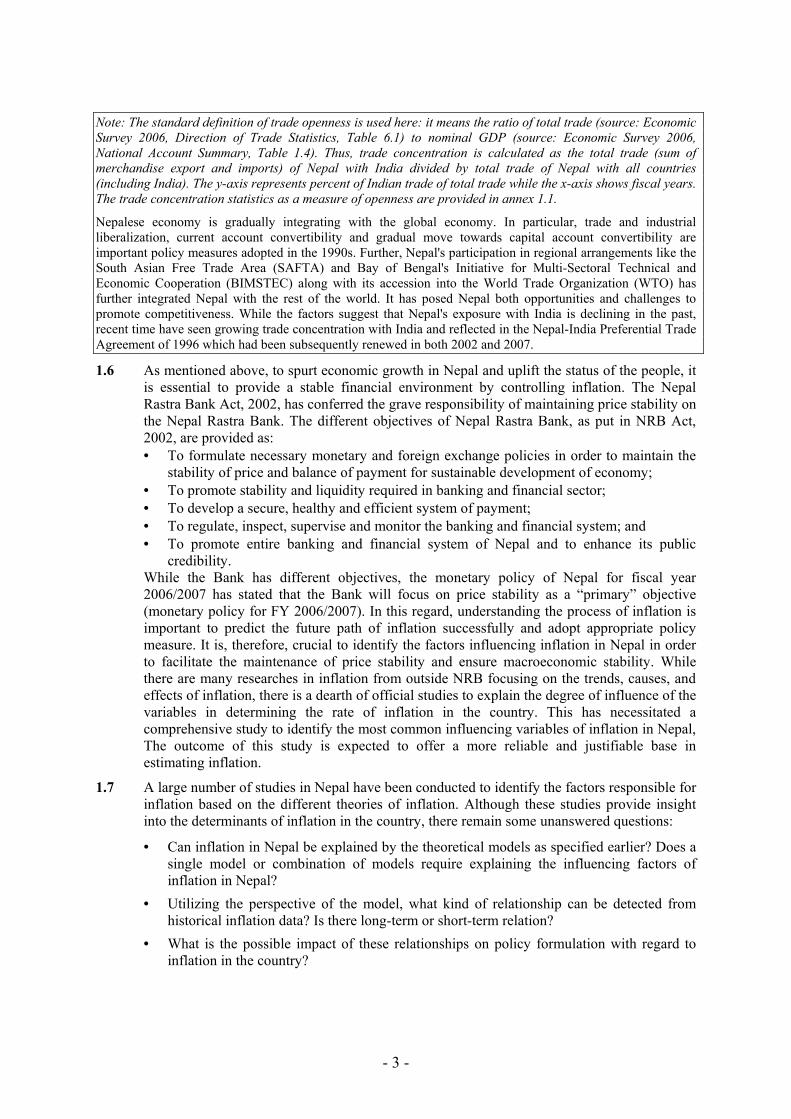
The geographical situation of porous border of about 1800 km. and the huge relative size of Indian economy has made Indian economic policies having multiple effects on Nepalese economic policies. This can be seen by the 1950 Treaty of Trade and Transit as well as the present pegged exchange rate of the Nepalese Currency (NC) with Indian Currency (IC), which had commenced in 1960. This has resulted in the Nepalese economy having a dual nature - relatively close to the rest of the world but relatively open to India. The strong economic link between both countries is moreover reflected in extremely strong trade link2 as shown in the graph below.

Figure 2: Graph for trade concentration with India

.2

.3

.4

.5

.6

.7

.8

.9

1975 1980 1985 1990 1995 2000 2005

TRADECONCENTRATIONINDIA

Source: Nepal Rastra Bank

2 If informal trade between India and Nepal were taken into account, this figure would increase significantly.

- 3 -

Note: The standard definition of trade openness is used here: it means the ratio of total trade (source: Economic Survey 2006, Direction of Trade Statistics, Table 6.1) to nominal GDP (source: Economic Survey 2006, National Account Summary, Table 1.4). Thus, trade concentration is calculated as the total trade (sum of merchandise export and imports) of Nepal with India divided by total trade of Nepal with all countries (including India). The y-axis represents percent of Indian trade of total trade while the x-axis shows fiscal years. The trade concentration statistics as a measure of openness are provided in annex 1.1.

Nepalese economy is gradually integrating with the global economy. In particular, trade and industrial liberalization, current account convertibility and gradual move towards capital account convertibility are important policy measures adopted in the 1990s. Further, Nepal's participation in regional arrangements like the South Asian Free Trade Area (SAFTA) and Bay of Bengal's Initiative for Multi-Sectoral Technical and Economic Cooperation (BIMSTEC) along with its accession into the World Trade Organization (WTO) has further integrated Nepal with the rest of the world. It has posed Nepal both opportunities and challenges to promote competitiveness. While the factors suggest that Nepal's exposure with India is declining in the past, recent time have seen growing trade concentration with India and reflected in the Nepal-India Preferential Trade Agreement of 1996 which had been subsequently renewed in both 2002 and 2007.

1.6 As mentioned above, to spurt economic growth in Nepal and uplift the status of the people, it is essential to provide a stable financial environment by controlling inflation. The Nepal Rastra Bank Act, 2002, has conferred the grave responsibility of maintaining price stability on the Nepal Rastra Bank. The different objectives of Nepal Rastra Bank, as put in NRB Act, 2002, are provided as: • To formulate necessary monetary and foreign exchange policies in order to maintain the

stability of price and balance of payment for sustainable development of economy; • To promote stability and liquidity required in banking and financial sector; • To develop a secure, healthy and efficient system of payment; • To regulate, inspect, supervise and monitor the banking and financial system; and • To promote entire banking and financial system of Nepal and to enhance its public

credibility. While the Bank has different objectives, the monetary policy of Nepal for fiscal year

2006/2007 has stated that the Bank will focus on price stability as a “primary” objective (monetary policy for FY 2006/2007). In this regard, understanding the process of inflation is important to predict the future path of inflation successfully and adopt appropriate policy measure. It is, therefore, crucial to identify the factors influencing inflation in Nepal in order to facilitate the maintenance of price stability and ensure macroeconomic stability. While there are many researches in inflation from outside NRB focusing on the trends, causes, and effects of inflation, there is a dearth of official studies to explain the degree of influence of the variables in determining the rate of inflation in the country. This has necessitated a comprehensive study to identify the most common influencing variables of inflation in Nepal, The outcome of this study is expected to offer a more reliable and justifiable base in estimating inflation.

1.7 A large number of studies in Nepal have been conducted to identify the factors responsible for inflation based on the different theories of inflation. Although these studies provide insight into the determinants of inflation in the country, there remain some unanswered questions:

• Can inflation in Nepal be explained by the theoretical models as specified earlier? Does a single model or combination of models require explaining the influencing factors of inflation in Nepal?

• Utilizing the perspective of the model, what kind of relationship can be detected from historical inflation data? Is there long-term or short-term relation?

• What is the possible impact of these relationships on policy formulation with regard to inflation in the country?

- 4 -

1.8 The present study is a modest attempt to answer these questions. The basic objective of the study is to identify the factors influencing inflation in Nepal. It includes the following specific objectives:

• To review major models of inflation and identify the appropriate model for Nepal; • To identify the short-term and long term relationship of inflation with the factors after

their identifications; and • To analyze the impact of determining variables in inflation

1.9 Regarding the methodology of the study, the general model of inflation for Nepal will be developed first after i) examining the historical pattern of inflation in Nepal, ii) viewing different theories of inflation, and iii) reviewing the previous studies at national and international level, specially considering to the methodological aspects and different tools. Different variables will be identified to incorporate into the general model. The span of the data for the study will be made consistent from fiscal year 1975/76 to fiscal year 2005/2006.3 Unit root test will be performed to identity the order of integration of the variables, followed by ordinary least square method to run the regressions of the general model. Then, the specific model will be developed through the method of elimination applying the wild test techniques. This covers a short run equation for the inflation processes in Nepal. To capture the inflation dynamics in the country, the long-run equation will be developed through cointegration and error correction techniques. The error correction model will be then utilized using both the long-term relationship between the inflation and identified variable; and error correction term – deviation from the long term dynamics in the short-run. The conclusion thus obtained will be tested for robustness using different alternative ways.

1.10 Being comprehensive in coverage, there are inherent limitations in the study for various reasons. Firstly, high frequency data (e.g. monthly, quarterly etc.) are not used in this study because of unavailability of some of the important data. Specifically, national accounts statistics in Nepal are compiled on annual basis. Second, the monetary figures may not accurately capture the level of domestic currency in circulation because of the circulation of significant volume of Indian currency. For example, Sharma (1998) has estimated that the presence of Indian currency is 40.72% of the overall business transactions in the country,

1.11 The study proceeds as follows. Chapter 2 provides historical overview of inflation along with its decompositions. Different theories and models of inflation are explained in Chapter 3. Chapter 4 attempts to review literatures and empirical findings in the context of different economies to identify relationship and develop estimation techniques. A vigorous exercise will be conducted to identify different influencing factors in Chapter 5 that applies estimation and modeling procedure on inflation in Nepal. This empirical work is followed by the chapter 6 with a detailed analysis and policy implications of the empirical exercises. Summary, conclusion and some recommendatory aspects are highlighted in chapter 7.

3 For ease of representation, the study will use the end year to represent the fiscal year - thus fiscal year 1975/76 will

be simply represented by 1976.

- 5 -

2 Historical Overview of Inflation in Nepal

The price level and its growth, inflation, is an important economic indicator. There are various indices which measure the price level, such as; consumer price index (CPI): wholesale price index (WPI); sensitive price index (SPI); gross domestic product (GDP) deflator and so on. In Nepal, there are three main price indices, namely: the CPI; the WPI; and the Salary and Wage Rate Index (SWRI). 4 The main focus for measuring the cost of living is placed on CPI. This is because CPI measures inflation impact which is the final measure of prices on households. This chapter, therefore, overview the historical development and trend of CPI in Nepal. The chapter is broken down into three sections: the next section discusses the composition and structure of CPI in Nepal followed by historical perspectives of inflation and decomposition of inflation trends.

2.1 Composition and structure of CPI in Nepal NRB is the domestic authority which collects price information and construct CPI index.5 The

CPI index captures the average household's consumption basket. This basket is determined by national level Household Budget Surveys (HSB). The objective of the survey is to make more representative basket in terms of cities, markets, items and weights for different commodities, income and occupation of the people. NRB has conducted three Household Budget Surveys (HBS) during 1972/73, 1984/85 and 1995/96 respectively; the basic compositions and relative weightage of the different commodities and services for the three completed HBS are provided in annex 2.3. Likewise, the fourth survey is presently under progress and purposes to address the shortcoming of previous HBS of being urban-focused and hence suggests to include the rural market centers. The comparative statements of the different household budget surveys are provided below:

Table 2.1: Comparative statement of the Household Budget Survey

Subject First HBS Second HBS Third HBS Fourth HBS*

Survey Period 1972/73 1983/84 1995/96 2005/06

Coverage Rural+ Urban Rural + Urban Urban Only Rural + Urban

Number of Market Centers 18 35 (12 Urban, 23 Rural) 21 52 (23 Urban, 29 Rural)

Sample Households 6,625 5,323 2,500 5,095

Population of the country 11,555,983 15,022,839 18,491,097 23,151,423

No. of Households of the country 2,084,062 2,584,948 3,328,721 4,253,220 *Proposed

Source: Nepal Rastra Bank

Presently, NRB constructs a number of price indices using the composition from the third HSB. These are namely: National Urban CPI, CPI for Kathmandu Valley, CPI for Hills, and CPI for Terai. The CPI basket for Kathmandu Valley consists of 301 items, while it includes 284 and 267 items in the Hills and the Terai regions respectively. The study looks at the National Urban CPI-the official measure used by NRB, to represent domestic price level.

The inflation statistics from the period 1976 – 2006 is shown in table below, with the statistics of the major components of the basket presently being used by NRB (from 3rd HSB).

4 For information on these measures of inflation and core measure of CPI, see the annex 2.1. 5 History of price collection at Nepal is provided in annex 2.2

- 6 -

Table 2.2: Inflation performance over the period 1976 - 2006

Items Mean Std. Dev. Volatility* Overall Inflation 8.23 4.61 0.56 Food and Beverage 8.17 6.47 0.79 1 Cereal Products 7.43 10.22 1.38 Rice 7.48 10.77 1.44 2 Pulses 9.56 11.41 1.20 3 Fruits and Vegetables 9.24 9.44 1.02 4 Spices 9.09 15.02 1.65 5 Meat, Fish and Eggs 9.04 4.76 0.53 6 Milk and Milk Products 8.55 5.45 0.64 7 Edible Oil and Ghee 8.20 14.73 1.80 8 Sugar and Sugar Products 7.68 14.52 1.89 9 Beverages 8.35 7.03 0.84 10 Restaurant Meals 10.33 8.37 0.81 Non-food and Services 8.39 2.85 0.34 1 Cloth, Clothes and Sewing 6.84 3.74 0.55 Clothes 6.08 4.62 0.76 Sewing 7.10 3.96 0.56 2 Footwear 6.08 4.22 0.69 3 Housing 9.98 3.63 0.36 Fuel, Light and Water 11.64 6.22 0.53 4 Transport and Communication 8.52 4.76 0.56 5 Medical and Personal Care 7.15 3.90 0.55 6 Education, reading and Recreation 8.77 5.47 0.62 7 Tobacco and Cigarettes 6.85 4.82 0.70

* Volatility, also taken to be coefficient of variation, is defined as the ratio of standard deviation of individual component of the CPI to its mean.

Source: Quarterly Economic Bulletin, NRB

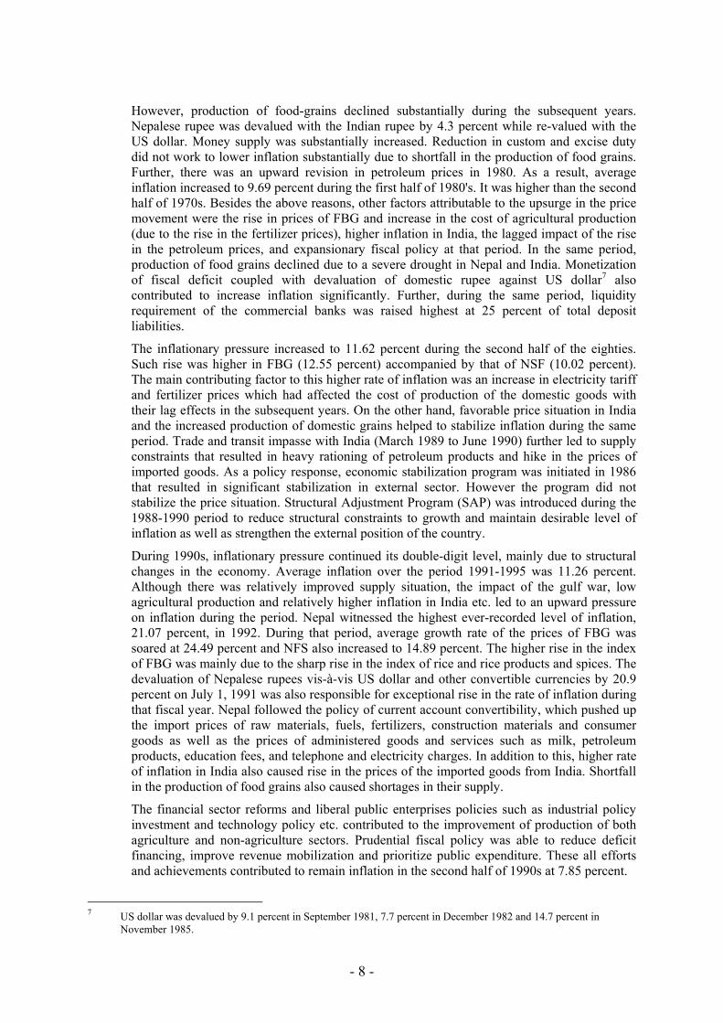
Over the period from 1976 to 2006, average rate of inflation remained at 8.23 percent. This growth rate is decomposed into growth rate of Food and Beverage group (FBG) and that of Non-food and Services (NFS) group which was 8.17 percent and 8.39 percent respectively. Similarly, the prices of FBG have been observed more volatile over the period compared to NFS, being 0.79 for the former and 0.34 for the latter group. Similarly, standard deviation of overall CPI and that for FBG and for NFS were 4.61, 6.47 and 2.85 respectively. Within the FBG itself, the prices of cereal products, pulses, vegetables and fruits, spices, edible oil and ghee, and sugar and related products were more volatile.

2.2 Historical Perspective of inflation in Nepal Measurement of prices in Nepal began from 1973 using the expenditure weightage of the

goods and services of the people obtained from first HBS. Prior to that, equal weights were

- 7 -

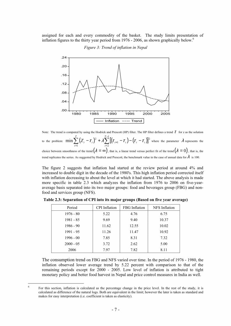
assigned for each and every commodity of the basket. The study limits presentation of inflation figures to the thirty year period from 1976 - 2006, as shown graphically below.6

Figure 3: Trend of inflation in Nepal

.00

.04

.08

.12

.16

.20

.24

1980 1985 1990 1995 2000 2005

Inflation Trend

Note: The trend is computed by using the Hodrick and Prescott (HP) filter. The HP filter defines a trend τ for z as the solution

to the problem: ( ) ( ) ( )[ ]∑ ∑=

−

== −−−+−

T

t

T

tttttttZ

1

1

2

21

2min ττττλτ where the parameter λ represents the

choice between smoothness of the trend ( )∞=λ , that is, a linear trend versus perfect fit of the trend ( )0=λ , that is, the

trend replicates the series. As suggested by Hodrick and Prescott, the benchmark value in the case of annual data for λ is 100.

The figure 2 suggests that inflation had started at the review period at around 4% and

increased to double digit in the decade of the 1980's. This high inflation period corrected itself with inflation decreasing to about the level at which it had started. The above analysis is made more specific in table 2.3 which analyzes the inflation from 1976 to 2006 on five-year-average basis separated into its two major groups: food and beverages group (FBG) and non-food and services group (NFS).

Table 2.3: Separation of CPI into its major groups (Based on five year average)

Period CPI Inflation FBG Inflation NFS Inflation 1976 - 80 5.22 4.76 6.75 1981 - 85 9.69 9.40 10.37 1986 - 90 11.62 12.55 10.02 1991 - 95 11.26 11.47 10.92 1996 - 00 7.85 8.31 7.32 2000 - 05 3.72 2.62 5.00

2006 7.97 7.82 8.11 The consumption trend on FBG and NFS varied over time. In the period of 1976 - 1980, the

inflation observed lower average trend by 5.22 percent with comparison to that of the remaining periods except for 2000 - 2005. Low level of inflation is attributed to tight monetary policy and better food harvest in Nepal and price control measures in India as well.

6 For this section, inflation is calculated as the percentage change in the price level. In the rest of the study, it is

calculated as difference of the natural logs. Both are equivalent in the limit; however the later is taken as standard and makes for easy interpretation (i.e. coefficient is taken as elasticity).

- 8 -

However, production of food-grains declined substantially during the subsequent years. Nepalese rupee was devalued with the Indian rupee by 4.3 percent while re-valued with the US dollar. Money supply was substantially increased. Reduction in custom and excise duty did not work to lower inflation substantially due to shortfall in the production of food grains. Further, there was an upward revision in petroleum prices in 1980. As a result, average inflation increased to 9.69 percent during the first half of 1980's. It was higher than the second half of 1970s. Besides the above reasons, other factors attributable to the upsurge in the price movement were the rise in prices of FBG and increase in the cost of agricultural production (due to the rise in the fertilizer prices), higher inflation in India, the lagged impact of the rise in the petroleum prices, and expansionary fiscal policy at that period. In the same period, production of food grains declined due to a severe drought in Nepal and India. Monetization of fiscal deficit coupled with devaluation of domestic rupee against US dollar7 also contributed to increase inflation significantly. Further, during the same period, liquidity requirement of the commercial banks was raised highest at 25 percent of total deposit liabilities.

The inflationary pressure increased to 11.62 percent during the second half of the eighties. Such rise was higher in FBG (12.55 percent) accompanied by that of NSF (10.02 percent). The main contributing factor to this higher rate of inflation was an increase in electricity tariff and fertilizer prices which had affected the cost of production of the domestic goods with their lag effects in the subsequent years. On the other hand, favorable price situation in India and the increased production of domestic grains helped to stabilize inflation during the same period. Trade and transit impasse with India (March 1989 to June 1990) further led to supply constraints that resulted in heavy rationing of petroleum products and hike in the prices of imported goods. As a policy response, economic stabilization program was initiated in 1986 that resulted in significant stabilization in external sector. However the program did not stabilize the price situation. Structural Adjustment Program (SAP) was introduced during the 1988-1990 period to reduce structural constraints to growth and maintain desirable level of inflation as well as strengthen the external position of the country.

During 1990s, inflationary pressure continued its double-digit level, mainly due to structural changes in the economy. Average inflation over the period 1991-1995 was 11.26 percent. Although there was relatively improved supply situation, the impact of the gulf war, low agricultural production and relatively higher inflation in India etc. led to an upward pressure on inflation during the period. Nepal witnessed the highest ever-recorded level of inflation, 21.07 percent, in 1992. During that period, average growth rate of the prices of FBG was soared at 24.49 percent and NFS also increased to 14.89 percent. The higher rise in the index of FBG was mainly due to the sharp rise in the index of rice and rice products and spices. The devaluation of Nepalese rupees vis-à-vis US dollar and other convertible currencies by 20.9 percent on July 1, 1991 was also responsible for exceptional rise in the rate of inflation during that fiscal year. Nepal followed the policy of current account convertibility, which pushed up the import prices of raw materials, fuels, fertilizers, construction materials and consumer goods as well as the prices of administered goods and services such as milk, petroleum products, education fees, and telephone and electricity charges. In addition to this, higher rate of inflation in India also caused rise in the prices of the imported goods from India. Shortfall in the production of food grains also caused shortages in their supply.

The financial sector reforms and liberal public enterprises policies such as industrial policy investment and technology policy etc. contributed to the improvement of production of both agriculture and non-agriculture sectors. Prudential fiscal policy was able to reduce deficit financing, improve revenue mobilization and prioritize public expenditure. These all efforts and achievements contributed to remain inflation in the second half of 1990s at 7.85 percent.

7 US dollar was devalued by 9.1 percent in September 1981, 7.7 percent in December 1982 and 14.7 percent in

November 1985.

- 9 -

During 2001 - 2005, inflation was stabilized at 3.72 percent. Favorable weather condition improved the production of food articles at that period. It led to a smooth supply situation and helped to contain the prices of FBG at 2.62 percent, while that of NFS contained at 5.00 percent. However, the hike in the prices of petroleum products, lag effect of revision in the VAT rate during 2005 and poor supply situation due both to unfavorable weather condition as well as deteriorated law and order situation caused inflationary pressure in 2006 at a level of 8.0 percent.

2.3 Decomposition of inflation Time series of price index can be decomposed into basic components to facilitate analysis of

driving factors. In general, there consists of four components, namely: (i) seasonal, (ii) cyclical, (iii) trend, and (iv) random. Seasonal components reflect the fixed effects due to specific time of a year. Demand and supply patterns may be affected by seasonal components like weather, festivals, customs or holidays or other events within a year. Cyclical components have long periodicity ranging from five to seven years, attributed to business cycles in the economy. The trend component of a time-series shows the general tendency of the non-recurring movement of the series over a long period of time. Random components are error terms which reflect erratic fluctuations with no pattern, or totally unexplained variations. The irregular or random component refers to non-recurring movements, which have no specific cause. Seasonal adjustment simplifies data so that they may be interpreted more easily and without significant loss of information. It can be taken as part of the model itself rather than externally adjusting time series.

Use of additive or multiplicative seasonal components and direct and indirect method in the seasonal adjustment are critical while deciding for seasonal adjustment process. It is obvious that the multiplicative method reduces the additive model by logarithmic transformation of the original series. A model-based approach can probably accurately explore the trend, cyclical and irregular elements by performing a univariate decomposition of the series. An autoregressive integrated moving average (ARIMA) model based method is applied to decompose the price series into various unobserved components. The methodology for computing unobserved components of inflation is taken from (Domac and Elbirt, 1998). The study decomposed inflation for Albania into sub-patterns that identify each component separately. A univariate decomposition of the series on monthly data is applied through which the seasonality component was included. As present study looks at annual data, seasonality is taken to be unitary. The general mathematical representation is thus written as:

( )tttt RCTfp ,,=

Where pt is CPI inflation8 at period t; Tt is the trend component at period t; Ct is the cyclical component at period t; and Rt is the random component (or error) at period t. As the multiplicative form is the most commonly used functional relationship to relate these sub-patterns, it can be expressed as:

tttt RCTp ××=

Where pt represents the actual (observed) values of inflation. The purpose of decomposition is to identify Tt, Ct, and Rt by analyzing the original data p. More specifically this can be done by calculating moving averages and can be specified as:

tt CTMA ×=

8 Inflation is computed as the change in the natural log of the CPI.

- 10 -

Where MA is a moving average over a determined period and Tt is the trend.9 For this study, MA is taken to be two year moving averages while Tt is computed as earlier. Further, the ratio of p to MA will yield:

ttt

ttt RCT

RCTMA

p =×

××=

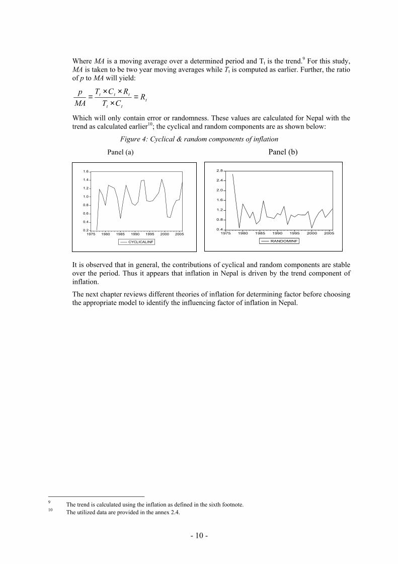
Which will only contain error or randomness. These values are calculated for Nepal with the trend as calculated earlier10; the cyclical and random components are as shown below:

Figure 4: Cyclical & random components of inflation

Panel (a) Panel (b)

It is observed that in general, the contributions of cyclical and random components are stable over the period. Thus it appears that inflation in Nepal is driven by the trend component of inflation.

The next chapter reviews different theories of inflation for determining factor before choosing the appropriate model to identify the influencing factor of inflation in Nepal.

9 The trend is calculated using the inflation as defined in the sixth footnote. 10 The utilized data are provided in the annex 2.4.

0.2

0.4

0.6

0.8

1.0

1.2

1.4

1.6

1975 1980 1985 1990 1995 2000 2005

CYCLICALINF

0.4

0.8

1.2

1.6

2.0

2.4

2.8

1975 1980 1985 1990 1995 2000 2005

RANDOMINF

- 11 -

3 Theories of Inflation

Understanding the cause of price rises is essential to control inflation. Unfortunately for policy makers, the economic literature has a plethora of explanations which attempt to explain the causes of price rise in the economy. The wide range of explanations is due to differences in underlying assumptions, such as on market efficiency, economic development etc. In this chapter, the seven major theories of inflation are reviewed; with relevant theories in the conclusion for appropriate to explain the price behavior in Nepal.

3.1 The quantity theory of money (QTM) Classical and neoclassical economists believe that the only way to price rises, and hence

inflation, is through the over-supply of quantity of money in an economy. If money is doubled, price also doubles in full employment situation where money plays as a means of transaction only. The well-known equation of exchange that explains QTM is:

MV = PT -------------------------------------------------------------------------- (1)

Where, M is money supply; V is the velocity of money, which is the measure of number of times one unit of money crosses the hands from one transaction to another; P is the general price level; and T represents the real volume of transactions.

In classical system, both V and T are assumed to be constant in the short run and hence the above equation of exchange can be rewritten to yield a price equation for the economy as follows:

TMVP /*= ------------------------------------------------------------------------ (2)

It simply states that doubling the money supply doubles the price level, proportionate relationship between quantity of money and price.

If we take the natural logarithm and differentiate the above equation, we can get the percentage change of the above variables as:

mg +−= )(νπ ---------------------------------------------------------------------- (3)

Where π, v, g and m represent the percentage changes in P, V, T, and M, respectively.

With V and T constants, both v and g are zero and hence inflation equals the growth rate of money supply. This states that inflation is only a monetary phenomenon and therefore, only reduction in money supply could fight against inflation in simple classical or neoclassical relationship.

The modern QTM accepts that inflation occurs when the rate of growth of the money supply exceeds the growth rate of the real aggregate output in the economy. According to the monetarists, the QTM implies that inflation is always, everywhere a monetary and demand-side phenomenon. In their view, cost-push arguments for inflation are misleading because they primarily are based on some microeconomic observations on the supply-side. Monetarists believe in general that the firm-specific cost increase cannot be inflationary as long as they are not related to, or accommodated by, increases in the money supply. Thus, the causation runs from inflation to costs, and not vice versa.

- 12 -

3.2 Demand-pull theory of inflation According to this theory, inflation is generated by pressure of excess demand of goods and

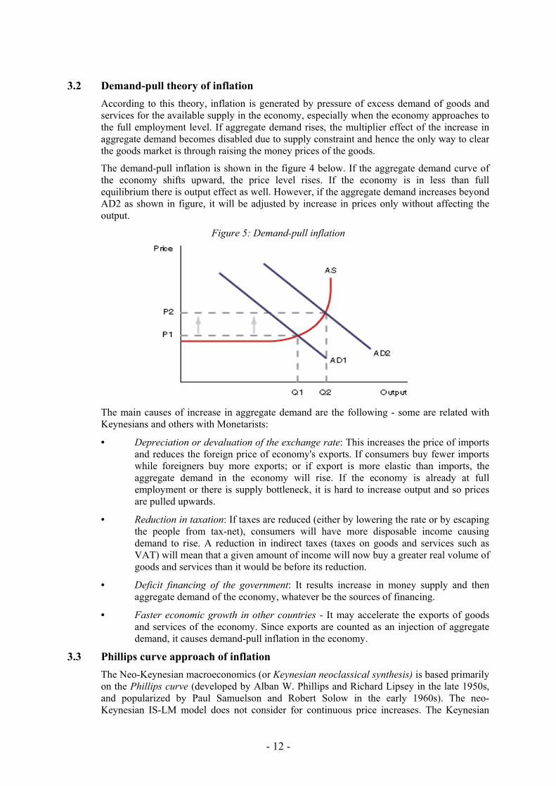
services for the available supply in the economy, especially when the economy approaches to the full employment level. If aggregate demand rises, the multiplier effect of the increase in aggregate demand becomes disabled due to supply constraint and hence the only way to clear the goods market is through raising the money prices of the goods.

The demand-pull inflation is shown in the figure 4 below. If the aggregate demand curve of the economy shifts upward, the price level rises. If the economy is in less than full equilibrium there is output effect as well. However, if the aggregate demand increases beyond AD2 as shown in figure, it will be adjusted by increase in prices only without affecting the output.

Figure 5: Demand-pull inflation

The main causes of increase in aggregate demand are the following - some are related with

Keynesians and others with Monetarists:

• Depreciation or devaluation of the exchange rate: This increases the price of imports and reduces the foreign price of economy's exports. If consumers buy fewer imports while foreigners buy more exports; or if export is more elastic than imports, the aggregate demand in the economy will rise. If the economy is already at full employment or there is supply bottleneck, it is hard to increase output and so prices are pulled upwards.

• Reduction in taxation: If taxes are reduced (either by lowering the rate or by escaping the people from tax-net), consumers will have more disposable income causing demand to rise. A reduction in indirect taxes (taxes on goods and services such as VAT) will mean that a given amount of income will now buy a greater real volume of goods and services than it would be before its reduction.

• Deficit financing of the government: It results increase in money supply and then aggregate demand of the economy, whatever be the sources of financing.

• Faster economic growth in other countries - It may accelerate the exports of goods and services of the economy. Since exports are counted as an injection of aggregate demand, it causes demand-pull inflation in the economy.

3.3 Phillips curve approach of inflation The Neo-Keynesian macroeconomics (or Keynesian neoclassical synthesis) is based primarily

on the Phillips curve (developed by Alban W. Phillips and Richard Lipsey in the late 1950s, and popularized by Paul Samuelson and Robert Solow in the early 1960s). The neo-Keynesian IS-LM model does not consider for continuous price increases. The Keynesian

- 13 -

neoclassical synthesis incorporated labor market dynamics into the IS-LM model by taking into account the Phillips Curve (PC) to eliminate the missing wage/price block, or inflation equation, in the system:

U+= απ ---------------------------------------------------------------------------------- (4a)

Where π represents the inflation rate and U is the unemployment rate. The trade-off, or negative correlation, between inflation and unemployment was stated by α < 0. That is, the higher the inflation rate the lower is the unemployment rate, and vice versa. Furthermore, an increase in the inverse of U, or simply a decrease in U, was interpreted as an indication for excess demand in labor and hence in goods markets, following the demand-pull explanation for inflation.

The demand-side determination of inflation within the IS-LM-PC framework, however, failed to explain stagflation in the late 1960s and 1970s. The oil-price shocks in the 1970s caused global recessionary and cost-push inflationary effects at the same time. The observed evidence on incompatibility between the PC relationship and the co-existence of stagnation and inflation was actually predicted by monetarist economists such as Milton Friedman and Edmund Phelps who proposed a so-called expectations-augmented PC in the late 1960s:

eU βπαπ += . ------------------------------------------------------------------------------ (4b)

Where πe is inflation expectations and β represents the expectation adjustment parameter. In the short-run, there is still a negative relationship between inflation and unemployment for a given πe. That is, inflation expectations act as a shift variable in the model. However, assuming that β=1 and πe

= π in the long run, the PC must be vertical according to the monetarist critique of the standard PC. In other words, there is no trade-off between π and U in the long run, and the vertical long-run PC represents a kind of “natural rate of unemployment”.

According to the monetarists, the formation of inflation expectations is backward looking, or adaptive. Because all information is not available to economic agents during their formation of price expectations:

ett

et 11 )1( −− −+= πλλππ ------------------------------------------------------------------- (5)

Where λ and (1-λ) are the adjustment parameters, or weights. Equation (7) states that the expected rate of inflation at time t is only a weighted average of the actual inflation rate and the expected inflation rate in the previous period. This equation of expectations is interpreted as an appropriate measure of inflation inertia. The concept of backward-looking (or less informed) expectations is also used by as a major determinant of money demand in his famous analysis of hyperinflation (Phillip Cagan 1956).

3.4 Cost-push theories of inflation Cost-push theories of inflation largely attribute inflation to non-monetary, supply-side effects

that change the unit cost and profit markup components of the prices of individual products (Humphrey, 1998). Cost-push inflation occurs due to increase in cost of production of goods and services in the economy. Sometimes costs may increase simply due to economic booming, for example, increase in general wages because of rapid expansion in demand. This is demand-pull inflation rather than cost-push because increases in wages are simply the reaction of the market pressure in demand. Therefore, it is important to look at why costs have increased.

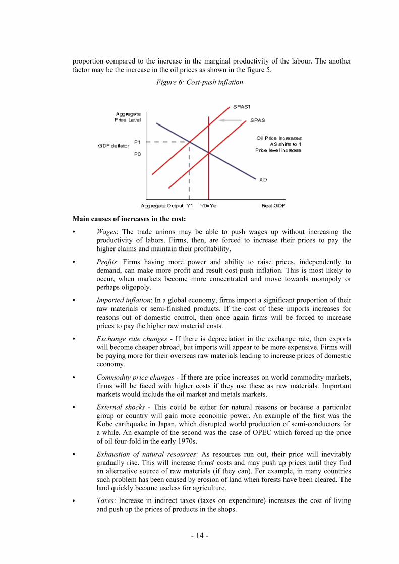
Cost-push inflation can be shown using the aggregate demand and aggregate supply curves. In this case, it is not the aggregate demand that increases; it is the aggregate supply curve that shifts to the left as a result of the increase in the cost of production. The cost of production can be increased if there is wage rate increment from the trade union power in greater

- 14 -

proportion compared to the increase in the marginal productivity of the labour. The another factor may be the increase in the oil prices as shown in the figure 5.

Figure 6: Cost-push inflation

Main causes of increases in the cost:

• Wages: The trade unions may be able to push wages up without increasing the productivity of labors. Firms, then, are forced to increase their prices to pay the higher claims and maintain their profitability.

• Profits: Firms having more power and ability to raise prices, independently to demand, can make more profit and result cost-push inflation. This is most likely to occur, when markets become more concentrated and move towards monopoly or perhaps oligopoly.

• Imported inflation: In a global economy, firms import a significant proportion of their raw materials or semi-finished products. If the cost of these imports increases for reasons out of domestic control, then once again firms will be forced to increase prices to pay the higher raw material costs.

• Exchange rate changes - If there is depreciation in the exchange rate, then exports will become cheaper abroad, but imports will appear to be more expensive. Firms will be paying more for their overseas raw materials leading to increase prices of domestic economy.

• Commodity price changes - If there are price increases on world commodity markets, firms will be faced with higher costs if they use these as raw materials. Important markets would include the oil market and metals markets.

• External shocks - This could be either for natural reasons or because a particular group or country will gain more economic power. An example of the first was the Kobe earthquake in Japan, which disrupted world production of semi-conductors for a while. An example of the second was the case of OPEC which forced up the price of oil four-fold in the early 1970s.

• Exhaustion of natural resources: As resources run out, their price will inevitably gradually rise. This will increase firms' costs and may push up prices until they find an alternative source of raw materials (if they can). For example, in many countries such problem has been caused by erosion of land when forests have been cleared. The land quickly became useless for agriculture.

• Taxes: Increase in indirect taxes (taxes on expenditure) increases the cost of living and push up the prices of products in the shops.

- 15 -

The structuralist approach to inflation is one of the major versions of the cost-push theories of inflation. The structuralist inflation models (developed in the 1960s) explain inflation with the productivity differences between the industrial and agricultural sectors. In general the traditional sector responds to monetary (or aggregate-demand) shocks with a lag. This lag is accompanied by a partial increase in industrial output and employment in the short run, which in turn increases wages and hence the demand for agricultural products. This increase implicates a change in relative prices in favor of foodstuffs. Higher agricultural prices lead to higher wage demands in this sector. Increasing wages increase the demand for industrial products, and the mechanism continues to work. In this model, aggregate supply chronically lags behind aggregate demand as a result of the temporary output rigidities in one of the sectors. Therefore, the structuralist model is accepted as a cost-push theory.

3.5 Rational expectations (RE) theory of inflation This theory has been formulated by John Muth and is supported by new classical economists

such as Robert E. Lucas, Thomas J. Sargent, Neil Wallac etc. This theory states that individuals and companies, acting with complete access to the relevant information, forecast inflation in the future without bias. Errors on their forecasts are assumed to result from random components.

Unlike in adaptive expectation principle, people do not consistently make the same prospect. Economic agents form their macroeconomic expectations “rationally” based on all past and current relevant information available, and not only on past information. The expectations are, however, totally random, or independent of each other. The RE approach to the business cycle and prices generated a vertical PC both for the short- and the long run. If the monetary authority announces a monetary stimulus in advance, people expect that prices rise.

Fully anticipated monetary policy cannot have any real effects even in the short-run. Thus, the central bank can affect the real output and employment only if it can find a way to create a price surprise. Otherwise, forward-looking expectation adjustments of economic agents will fail the pre-announced policy. Likewise, if a disinflation policy is announced in advance, it cannot reduce prices if people do not believe that the government will really carry it out. That is price expectations are closely related to the policy credibility and reputation for successful implementation.

3.6 Real business theory of inflation The real business cycle (RBC) theorists (such as Edward C. Prescott, Finn E. Kydland and

Charles I. Plosser) argued that upswings and downswings in economic activity originate from real (or aggregate supply) shocks rather than monetary (or aggregate demand) shocks. It assumes fixed aggregate demand curve, continuous market clearing, imperfect information, and rationality of expectations. The effects of supply shocks (e.g., process and production innovations, discovery of new sources of raw materials, changes in relative prices of foods and energy, bad weather, and nominal effective exchange rate changes) cause inflation, which is based on the business cycle.

It does not, however, explicitly explain inflation; rather, it particularly focuses on real output effects of adverse, or negative, supply shocks such as deviations of factor productivity from trend or relative price changes caused by oil price shocks. However, the main contribution of RBC economists is that they call our attention to the possibility of the important role of supply shocks in explaining inflation.

Neoclassical, monetarist and new classical economists ignored the possibility of adjustment lags.

3.7 New political economy theory of inflation The theories as mentioned above mainly focus on macroeconomic determinants of inflation

(e.g., monetary and real shocks, and inertia in inflation) and simply ignore the role of non-

- 16 -

economic factors such as institutions, political process and culture in process of inflation. They also overlook the possibility that sustained government deficits may be partially or fully endogenized by considering the effects of the political process and possible lobbying activities on government budgets, and thus, on inflation. Political forces, not the social planner, choose economic policy in the real world. Economic policy is the result of a decision process that balances conflicting interests so that a collective choice may emerge (Drazen, 2000). It, therefore, provides fresh perspectives on the relations between timing of elections, policymaker performance, political instability, policy credibility and reputation, central bank independence and the inflation process itself.

3.8 Conclusion The review of major theories on causes of inflation reiterate that inflation process is country

specific; that is factors such as political, institutional, and cultural changes may be crucial while modeling to inflation. In general, most economists agree that inflation in the long run is due to excess money supply. However, this is not applicable to all economies, especially developing countries like Nepal. Looking over the historical overview of inflation in Nepal, it is felt that structural factors along with monetary factors also play a significant role in shaping inflation. The following chapter reviews empirical literature on inflation and provides information for deciding on the empirical methodology to be used in the later part of the study.

- 17 -

4 Literature Review

There are large numbers of empirical exercises, which attempt to measure and understand the causes of inflation. For developing countries with embryonic financial sectors, a monetarist, demand-pull or structuralist theory of inflation may be more appropriate. This chapter attempts to review some empirical studies on inflation focusing on large groupings as well as those of individual country studies (both international and also national level studies). The chapter ends with some thoughts of the appropriate empirical methodology for the study.

4.1 There are some studies which examine inflation processes in the region as a whole - the group of countries taken together. For example, Vogel (1974) developed a monetary model for explaining inflation in Latin America. The author's model considered the rate of inflation (P

t)

as a dependent variable and the percentage change in money supply during current and previous years (M

t, and M

t-1), percentage change in real income during current period (Y

t) and

change in inflation rate lagged by one year and two years (Pt

and Pt-1

) as explanatory variables. Vogel (1974) concluded that the coefficients of M

t and M

t-1 are highly significant

and thus indicate that an increase in the rate of growth of money supply causes a proportionate increase in the rate of inflation within two years. At the same time the rate of inflation is found to be inversely influenced by the growth rate of real income. The rate of inflation is not found to be so much influenced by (P

t-1 – P

t-2), rather inflation rate lagged by

one year, Pt-1

has much influence on the current rate of inflation. The increase in the last equation above is mainly attributed to the high significance of P

t-1.

Similarly, McCandless and Weber (1995) looked at inflation in 110 countries during a 30-year period. The study concluded that inflation and monetary aggregates are positively correlated in the long run. However, as the time horizon shortens, the correlation falls. Campillo and Miron (1996) examine the determinants of inflation across 62 countries over the period 1973 - 1994 by considering the distaste for inflation, optimal tax considerations, time consistency issues, distortionary non-inflationary policies and other factors as important determinants of inflation. Inflation rate is measured by the Consumer Price Index (CPI). The authors' have adopted Ordinary Least Squares (OLS) technique with standard error, estimated by White (1980) procedure. They found economic fundamentals like economic openness and optimal tax considerations are relatively important determinants of inflation whereas institutional arrangements like central bank independence or exchange rate mechanisms are relatively less important.

4.2 Large studies of many countries taken at a time, although important for gaining general insights, have been found to loose out information on country-specific experiences. Because of this, country specific studies have become popular. Therefore, it is equally important to look at individual country-specific studies. Razzak (2001) examined the New Zealand experience from a monetary perspective and showed that the time series correlation between inflation and monetary aggregates was high only during high-inflation periods and disappeared when inflation was low. Likewise, Lissovolik (2003) examined the transitional economy of Ukraine from a monetary and structural perspective using monthly data over the period 1993 - 2002 and concluded that money, wage and exchange rate largely affect inflation. Maliszewski (2003) examined inflation-determinants in Georgia and the relationship between prices, money and exchange rate over the period 1996:1 to 2003:2. The

- 18 -

sutdy found that exchange rate is the dominant determinant of inflation. Also, Blavy (2004) examined the dynamic of inflation in Guinea using a simple monetary model. There are many other country studies around the world but focus is given on three studies which share similar situation to Nepal. These are the studies of Albania, Swaziland, and Pakistan.

4.3 The first study by Domac and Elbirt (1998) examine the behavior and determinants of inflation in Albania by employing three different approaches. Firstly, the authors decomposed inflation into four components: seasonal, cyclical, trend, and random. Secondly, they used Granger causality test on both the consumer price index (CPI) and key economic variables, to investigate their information content. And, lastly, they apply cointegration and error-correction techniques to the process of inflation to a monetary model. The model is expressed as :

ftttttt PePyMP loglogloglogloglog 1 γνδφα ++∆++= −

where P, M and e are price, money supply and exchange rates respectively. The authors conclude that (1) inflation exhibits strong seasonal patterns associated with agriculture seasonality with monetary aggregates matching inflation by lag of two-months and that the exchange rate also exhibits a stable seasonality pattern; (2) Granger causality test shows that M1 (currency in circulation plus demand deposits) and the exchange rate have predictive impact for most components of the CPI and that credit to government is a good predictor of medical care, transportation, and communication prices. The study finds that an increase in the fiscal deficit would undermine competitiveness by producing appreciation in the real exchange rate. (3) Lastly, the cointegration and error-correction model show that inflation is positively related to both money supply and the exchange rate and negatively related to real income in the long run. The impact of the exchange rate on inflation occurs a month later, while the impact of real income and money take place two and four months later respectively.

4.4 The second study by Dlamini et al (2001) attempts to identify the relevant influencing factors of inflation in Swaziland using both open monetary and structural variables over the period 1974 - 2000. The CPI of Swaziland is taken to be the dependent variable with the explanatory variables being the real income (Y), nominal money supply (M), nominal interest rate (R), nominal exchange rate (E), nominal wages (W) and South African consumer prices (SP). The estimated equation is thus:

tt6t5t4t3t2t1t WlnSPlnMlnElnRlnYlnlnPln µ+β+β+β+β+β+β+α= and );0(NID 2t σ=µ

Due to limitations of real sector data, annual time series are used. The authors apply cointegration technique and error correction model (ECM) to estimate relationship between inflation and its determinants. The study found that money supply and interest rate has insignificant influence on inflation. The coefficient of real income growth was also insignificant, though it was positive. However, foreign price (i.e. South African inflation) and exchange rate has a significant long-run influence in inflation. It was also found that a large interdependence between wages and inflation exist both in the short-and long run. The authors conclude that changes in the lagged exchange rate, South African inflation and nominal wages were major determinants of inflation in Swaziland.

4.5 Finally, the study by Khan and Shimmelpfinnig (2006) has examined the relative importance of monetary and supply side factors for inflation in Pakistan over the period 1998:1 to 2005:6. The model consists of money supply, credit to private sector and 6- month Treasury bill rate as monetary variables and nominal effective exchange rate, wheat prices guaranteed by the government as supply side factors. Both annual real and nominal GDP are interpolated to 12-month moving average as activity variable. The open economy generalized monetarist model includes administered wheat prices to reach at hybrid monetarist – structuralist model, which is given as:

),,,,,,( wervymfp &&&&&& =

- 19 -

Where a dot over a variable denotes growth rate (first derivative with respect to time), thus p is prices, m stands for money, y for real GDP, v is the velocity of money, r is interest rate, e is exchange rate and w is wheat support price. The variables are taken in the natural logarithm form. The authors estimate the above relation in both the short term and the long term using a Vector-Error Correction Model (VECM). The authors conclude that in the long run, monetary factors play a dominant role in inflation with a lag effect of one year, whereas administered prices influence inflation in the short-run only.

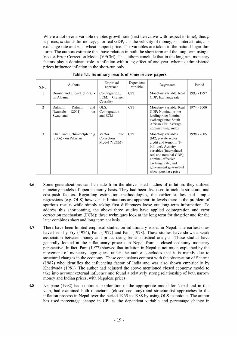
Table 4.1: Summary results of some review papers

S.No.

Authors Empirical approach

Dependent variable Regressors Period

1 Domac and Elbirdt (1998) - on Albania

Cointegration,, ECM, Granger Causality

CPI Monetary variable, Real GDP; Exchange rate

1993 - 1997

2 Dalmini, Dalmini and Nxumalo (2001) - on Swaziland

OLS, Cointegration and ECM

CPI Monetary variable, Real GDP; Nominal prime lending rate; Nominal exchange rate; South African CPI; Average nominal wage index

1974 - 2000

3 Khan and Schimmelpfennig (2006) - on Pakistan

Vector Error Correction Model (VECM)

CPI Monetary variables (M2, private sector credit and 6-month T-bill rate); Activity variables (interpolated real and nominal GDP); nominal effective exchange rate; and government guaranteed wheat purchase price

1998 - 2005

4.6 Some generalizations can be made from the above listed studies of inflation: they utilized monetary models of open economy basis. They had been discussed to include structural and cost-push factors. Regarding estimation methodologies, the earlier studies had simple regressions (e.g. OLS) however its limitations are apparent: in levels there is the problem of spurious results while simply taking first differences loose out long-term information. To address this shortcoming, the above three studies have applied cointegration and error correction mechanism (ECM); these techniques look at the long term for the prior and for the later combines short and long term analysis.

4.7 There have been limited empirical studies on inflationary issues in Nepal. The earliest ones have been by Fry (1974), Pant (1977) and Pant (1978). These studies have shown a weak association between money and prices using basic statistical analysis. These studies have generally looked at the inflationary process in Nepal from a closed economy monetary perspective. In fact, Pant (1977) showed that inflation in Nepal is not much explained by the movement of monetary aggregates, rather the author concludes that it is mainly due to structural changes in the economy. These conclusions contrast with the observation of Sharma (1987) who identifies the influencing factor of India and was also shown empirically by Khatiwada (1981). The author had adjusted the above mentioned closed economy model to take into account external influence and found a relatively strong relationship of both narrow money and Indian prices, with Nepalese prices.

4.8 Neupane (1992) had continued exploration of the appropriate model for Nepal and in this vein, had examined both monetarist (closed economy) and structuralist approaches to the inflation process in Nepal over the period 1965 to 1988 by using OLS technique. The author has used percentage change in CPI as the dependent variable and percentage change in

- 20 -

current money supply, money supply lagged by one and two years, percentage change in GDP, and the expected cost of holding money, percentage change in output in commodity producing sectors lagged by one year, percentage change in the import price index lagged by one year and percentage change in government budget deficit as the explanatory variables. The monetarist model includes the rate of growth (as indicated by a dot over the respective variables) of money supply (M), per capita income (Y), and expected cost of holding money (C) as explanatory variables of inflation. The model is given as:

t5t42t31t2t1t CYMMMP &&&&&& α+α+α+α+α+α= −−

Similarly, the structuralist model of inflation is examined by using agricultural bottleneck, foreign exchange constraints, and fiscal constraints. The model consists of one year lagged percentage change in output (Yt-1) and import price index (MPt), percentage change in government expenditure (GOVt) and expected cost of holding money (Ct), which is given as:

t4t31t21t1t CVGOPMYP &&&&& β+β+β+β+β= −−

The findings of the study suggested that monetary policy is an important instrument to control inflation. An increase in money supply in line with the growth of per capita GDP could help to control inflation. However, the study could not empirically provide superiority of one approach to the other in explaining inflation; rather it exhibits the broader perspective of the complexities of the inflationary process.

4.9 Subsequent to Neupane (1992), the Institute for Sustainable Development (ISD; 1994), in a study conducted for Nepal Rastra Bank, used an eclectic approach of the monetarist and structuralist views. The study had identified money supply, international prices (particularly Indian prices), exchange rate, real output, government expenditure and expectation factors as major sources of inflation in Nepal. Similarly, infrastructural bottlenecks, imperfect market condition and market oriented economic policies are also instrumental for inflation escalation. The study utilized simple regression analysis and find that the explanatory power of a closed economy monetarist model (where price is the function of money supply and real output) is very low; the study therefore included external variables of an open economy model of regression analysis which includes Indian wholesale price exchange rate, lagged effect of money supply, government expenditure as additional explanatory variable. ISD (1994) found that a 10 percent increase in Indian prices causes a more than 8 percent rise in domestic price level in Nepal. This conclusion of the influence of external factors is consistent with the study by Khatiwada (1981).

4.10 In this line, Khatiwada (1994) examined the inflation process in Nepal utilizing basis the quantity theory of money. Initially, results showed low explanatory power and suggested that there were other missing variables in the equation. When open economy variables, such as Indian inflation and the exchange rate, were included this showed significant increase in the explanatory power of the equation. The study had also included structural variables such as per-capita output and government expenditures, but those did not have a significant effect being "swamped" by the monetary variables. The study further looks at long-run analysis and finds that the best fit to be that of five year moving averages as shown below:

UIPIlnbQlnbMlnbbPln i3i2i110i ++++= ∆∆∆∆

Where "IPI" is the Import Price Index. The study finds that IPI is consistently significant and suggests that inflation in Nepal is influenced by open economy forces.

4.11 Moving away from focus on the monetary explanation of inflation in Nepal, Mathema (1998) has used an expectation augmented Phillips Curve approach to examine whether the nominal wage increases are the most significant sources of cost push inflation. The final equation used by the study is:

ε++++++= PEaPIaWaMaGDPRaaP 543210

- 21 -

Annual CPI inflation (P), real GDP growth (GDPR), change in money supply (narrowly defined; M), change in wages (W), change in imported price (PI) and change in price expectation (PE)11 are the variables where excess demand proxies for unemployment. The data for the study period is 1978/79 and 1995/96. OLS and unit root tests are performed for stationarity test of the variables chosen. The author finds the importance of several wage variables for influencing domestic inflation but surprisingly does not find significant effect of imported prices. The author attributes this to "absorption of the effect of WPII (whole sale prices of India) by the money wages of laborers in the homeland" (Mathema, 1998, p. 16). Granger Bivariate Causality Test finds unilateral causation from the rate of inflation to wages of agricultural and masonry labour while industrial wages causes inflation in Nepal.

4.12 In contrast to Mathema (1998), Pandey (2005) utilized an excess demand model of inflation and has applied OLS, stationarity test, cointegration technique and error correction modeling to study the determinants of inflation in Nepal. The study has identified money supply (both narrow and broad), real GDP, government expenditure, Indian inflation and exchange rate as explanatory variables influencing inflation, over the period 1973 to 2004. Although bivariate regression between price and the average money revealed significant relationship, the low explanatory power of the equation suggested inclusion of more variables. The author could not find any change in the explanatory power of the model while including public expenditure as well as real GDP, a supply side variable. In an open economy monetarist model, Indian prices and exchange rate with Indian rupees and US dollar are included; however, the explanatory power of the model is limited to 47 percent only. The study had then used the ECM to avoid the problem of loosing long-run information on data to reveal both short-term relationship and adjustment toward long run equilibrium. The model adopted was:

dLn(CPI) = β0+β1fdLn(X)+β3et-1+dt,

Where, X represents explanatory variables. Pandey (2005) has found long run relationship of inflation in Nepal with money supply (narrowly defined), Indian inflation and exchange rate with India (as explanatory variables) however the error-correction term was found not to be significant, suggesting that there is no short run adjustment with regard to inflation in Nepal.

4.13 In the latest study on inflation, Nepal Rastra Bank, Price Division and Economic Analysis Division (2006) in a very quick and simple study using open economy monetary model, has found Indian inflation to have a significant and near unitary effect on inflation in Nepal. This interpretation resulted from empirical regression utilizing Ordinary Least Square (OLS) on annual time series data over 1975 to 2006. The explanatory variables are growth rates of real GDP, money supply (both narrowly and broadly defined), interest rate on fixed deposit and Indian inflation. However, the deficiency of this quick study is that there was no further exercise regarding long-term relationships and thus considerations for short-term adjustment pathways.

11 The author defined this as the difference of one year lagged inflation and current year inflation.

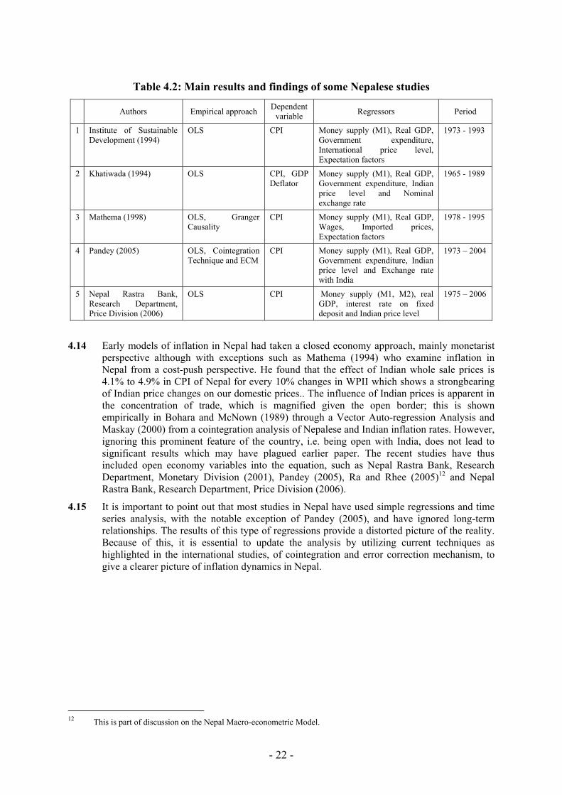
- 22 -

Table 4.2: Main results and findings of some Nepalese studies

4.14 Early models of inflation in Nepal had taken a closed economy approach, mainly monetarist

perspective although with exceptions such as Mathema (1994) who examine inflation in Nepal from a cost-push perspective. He found that the effect of Indian whole sale prices is 4.1% to 4.9% in CPI of Nepal for every 10% changes in WPII which shows a strongbearing of Indian price changes on our domestic prices.. The influence of Indian prices is apparent in the concentration of trade, which is magnified given the open border; this is shown empirically in Bohara and McNown (1989) through a Vector Auto-regression Analysis and Maskay (2000) from a cointegration analysis of Nepalese and Indian inflation rates. However, ignoring this prominent feature of the country, i.e. being open with India, does not lead to significant results which may have plagued earlier paper. The recent studies have thus included open economy variables into the equation, such as Nepal Rastra Bank, Research Department, Monetary Division (2001), Pandey (2005), Ra and Rhee (2005)12 and Nepal Rastra Bank, Research Department, Price Division (2006).

4.15 It is important to point out that most studies in Nepal have used simple regressions and time series analysis, with the notable exception of Pandey (2005), and have ignored long-term relationships. The results of this type of regressions provide a distorted picture of the reality. Because of this, it is essential to update the analysis by utilizing current techniques as highlighted in the international studies, of cointegration and error correction mechanism, to give a clearer picture of inflation dynamics in Nepal.

12 This is part of discussion on the Nepal Macro-econometric Model.

Authors Empirical approach Dependent variable Regressors Period

1 Institute of Sustainable Development (1994)

OLS CPI Money supply (M1), Real GDP, Government expenditure, International price level, Expectation factors

1973 - 1993

2 Khatiwada (1994) OLS CPI, GDP Deflator

Money supply (M1), Real GDP, Government expenditure, Indian price level and Nominal exchange rate

1965 - 1989

3 Mathema (1998) OLS, Granger Causality

CPI Money supply (M1), Real GDP, Wages, Imported prices, Expectation factors

1978 - 1995

4 Pandey (2005) OLS, Cointegration Technique and ECM

CPI Money supply (M1), Real GDP, Government expenditure, Indian price level and Exchange rate with India

1973 – 2004

5 Nepal Rastra Bank, Research Department, Price Division (2006)

OLS CPI Money supply (M1, M2), real GDP, interest rate on fixed deposit and Indian price level

1975 – 2006

- 23 -

5 Empirical Exercise

In the previous chapters, a historical analysis of inflation in Nepal was discussed as well as the different theories explaining the inflation dynamics and the techniques of estimating inflation. This chapter focuses on utilizing the previous experiences to undergo an empirical exercise for factors influencing inflation in Nepal. In this regard, the first section focuses on identifying the general model then moving towards a specific model for the country; the following sections provide regression analysis using both OLS method and error correction model (ECM) for determining both the-short run and long-run equation; and the final section ends with the interpretation of the regression analysis.

5.1 The previous chapters analyzed different models establishing the relationship between price levels and other variables. It was concluded that the selection of a particular model depends highly on the nature and structure of the economy. As a starting point and with consideration of developing and open nature of the economy, the exercise starts from that the model utilized by Nepal Rastra Bank (2006) to access the inflation process in the country. The model utilized by Nepal Rastra Bank (2006) is based on a monetary perspective. It had assumed that “individuals hold money either for transaction purposes, as a store of value, or for speculative purposes. In the model, for a constant velocity (v), inflation ( )p& results if money growth ( )m& exceeds real GDP growth ( )y& . Similarly, the interest rate (r) - the opportunity cost of holding money - reduces aggregate demand for money in the economy and leads to a reduced inflation. Moreover, financial deepening and innovations enable agents to use alternative monetary instruments in lieu of cash. Thus, the velocity of a particular monetary aggregate, say narrow money (M1), changes if individuals switch from cash to instruments included only in broad money (M2). In an open economy, headline inflation can also be affected by external factors such as the exchange rate or foreign inflation. In this regard, the factors in the general open-economy monetary model are given as:

( )extryvmfp ,,,,=

Where p, m, v, y, r and ext are price, money, velocity, GDP, interest rates and external factors respectively.13 For Nepal, Mathema (1998) has also found that a cost-push factor, namely workers' wages, is also important for influencing inflation in the country. In this regard, the above mentioned model will incorporate structural factor of wage rate and the hybrid form of model including both monetary as well as cost push factors, can be expressed as:

( )extwryvmfp ,,,,,=

This is the general model used by the study. 5.2 The conceptual variables mentioned in the above general model are specified through

operational variable. It should be pointed out that the time period of these variables are in terms of a fiscal year (FY) as identified by the Government of Nepal's (GON); a FY is the period from mid-July of one year to mid-July of the next year (e.g. FY 1999/2000 is mid-July 1999 to mid-July 2000). The variable description along with their sources, are provided below: • Price level in Nepal (p) is measured by the Consumer Price Index and is denoted by

PN, whose source is NRB; • The money supply (m) is measured by both narrow money (M1) and broad money

(M2) whose source is NRB;

13 This standard model is provided in many textbooks and most recently in the IMF Working Paper of Khan and Schimmelpfennig (2006), which utilize the above relationship as a basis for describing the inflation dynamics in Pakistan.

- 24 -

• Velocity (v) is calculated using the quantity theory of money: it is the ratio of nominal GDP to money (e.g. MV=PQ). If M1 is used then the velocity will be V1, if M2 is used then the velocity will be V2.14

• Real output (y) is measured by real GDP. The series is calculated from Nominal GDP series taken from Table 1.4 in the Government of Nepal's (GON) Economic Survey and deflated by the GDP deflator taken from same source.15

• Interest rate (r) is measured in three forms namely – 3-months fixed deposit rate of commercial banks, denoted by I1, commercial lending rate I2, and refinance rate of NRB, I3. All the series are taken from NRB;

• Wages (w) is measured by the monthly wages of the semi-skilled labors working in the industrial sector. The data series is obtained from the price division of Nepal Rastra Bank. Among the various wages, industrial wages has been taken as the representative because practically industrial wages seem to be revised as per the revision in salary of government sector and thereby causing demand-pull inflation in Nepal. Further, Mathema (1998) also observed that industrial wage affected Nepalese inflation among the different forms of wages the study had regressed.

• The external sector (ext) variable of the above model is proxied by Indian prices, PIn. This is because the model takes ext to reflect the effects of externalities in Nepalese inflation. In this regard, following two realities give the basis to choose Indian price level as a measurement of the external sector. First, Nepal has a stable pegged exchange rate with IC, with the last change taking place in February 12, 1993; second, Nepal has high concentration of trade with India as explained and portrayed in chapter 1, which is attributed to the open and contiguous border shared by both countries. Therefore, under the given rigid exchange rate and high concentration of trade between two countries, the Indian factor can be captured either through the exchange rate or through the Indian price level. It is felt that the rigid nature of the exchange rate does not convey much information; therefore Indian price level is utilized to capture the external factors of inflation. Box 2: The appropriate Indian price level for comparison with Nepalese CPI

Contrary to earlier national studies, this study does not use Indian Wholesale Price Index (WPI) as a measure of Indian price level for comparison with the Nepalese Consumer Price Index. In India there are many measures for calculating the national price level: three measures of the CPI, one measure of WPI etc. While the Reserve Bank of India takes WPI as the official measures of overall domestic price level in India it is important to point out that the different Indian price indexes do not move together: for example the Indian indexes of CPI (Industrial Workers) and WPI over the period 1978 - 2006, only have a coefficient correlation of 58.8%! While the domestic authority determines which index to target at the national level, for cross-country comparison it is essential to have comparable series. In Nepal's case, inflation is measured by CPI. The question is therefore, which Indian price index is appropriate for comparison with the Nepalese CPI? Although the majority of previous national level studies had taken WPI as a measure of Indian price level simply following the choice of the domestic authority (taken as tradition), the present study has decided not to utilize the WPI at the first instance (although used later on for test of robustness). This is because WPI looks at the price level at a different stage of the pricing process in comparison with CPI. That is, CPI is calculated from the retail levels from the different centers and hence measures the price levels of the ultimate consumers, on the other hand, WPI is obtained from wholesalers before reaching into the retail levels; hence WPI differs from the CPI to the extent of margin level and other addition of costs such as transportation etc. (example of this is starkly shown above with the correlation coefficient of the Indian CPI and WPI). As such, it was felt that using Indian WPI for comparing with Nepalese CPI is not justifiable. Furthermore, from the basket comparison point of view, Indian CPI has strong base for selection vis-à-vis Nepalese CPI compared to that of Indian WPI. If we compare the baskets of Indian WPI with Nepalese CPI, almost 45 percent weight (roughly calculated) of the Indian WPI basket is not represented by Nepalese CPI basket. All the three baskets: NCPI, ICPI and IWPI are provided in annex 5.2. Of the three indexes of CPI in India, the basket of industrial workers (measured from different cities of India) covers almost all of the goods and services presented in the Nepalese CPI basket. Therefore, out of three measures of Indian CPI, namely CPI for industrial workers; CPI for non-manual workers; and CPI for manual workers, Indian CPI for industrial workers is taken for comparison with the Nepalese CPI.

14 Calculation of VM1 and VM2 series is provided in annex 5.1 15 Calculation of RGDP series is provided in annex 5.1

- 25 -

• As elaborated in the above box the Indian CPI is taken as the appropriate Indian price level for comparison. The source of this Indian CPI is International Monetary Fund, (IFS code 64). There is no direct comparison of PIn with that of PN due to different reporting time frames: the fiscal year of the Government of Nepal ends on 15 July and all the series are based on this date. On the other hand, PIn is taken from the International Monetary Fund, (IFS code 64), which is based on calendar year (e.g. January to December). The differences in the dating convention have made it necessary to adjust Indian price level in the model to ensure comparability. Thus in calculating price for the current fiscal year, the prices for India was taken to be the average of the current and the previous calendar year price levels. For example PIn for fiscal year 2000 is 141.2 which is the simple average of the calendar years' value for 1999 and 2000 (being 138.4 and 144.0 respectively).

The original data series of the above-mentioned variables along with their summary statistics, for 28 year time spam from 1979 to 2006, are provided in annex 5.3; their graphs are provided in annex 5.4; the variables in log differences along with their summary statistics are provided in annex 5.5; and finally the graphs of the log differences variables are provided in annex 5.6.

5.3 The eleven identified variables are initially subject to time series analysis. This is because OLS technique of estimation is based on asymptotic convergence theorem, which assumes that the data series are stationary, i.e. mean and variances of the series are independent of the time. However, macroeconomic time series such as general price level, national output, money supply etc. generally have memory of the past and thus are non-stationary; this implies that they have a clear trend and hence have varying mean and variances over time. Treating such non-stationary series as stationary in OLS estimation will be biased and lead to failure in predicting outcomes; this will lead to spurious regressions where R-squared is approximately unity and t and F statistics look significant and valid. In order to avoid the problem of spurious regression, non-stationary data need to be made stationary, that is integrated of order zero, or I(0); differencing the series has become the common method to do this. If the series becomes stationary by its first difference, it is said to be integrated of order 1, I (1) and so on. The non-stationarity of series are checked through Augmented Dickey Fuller Test.16 The table 5.1 gives the t-statistics and associated p-values of the Dickey Fuller Test of the variables in the equations.

16 The ADF test takes into account of the intercept and the time trend with maximum lags equal to 4 to get rid of serial correlations problems

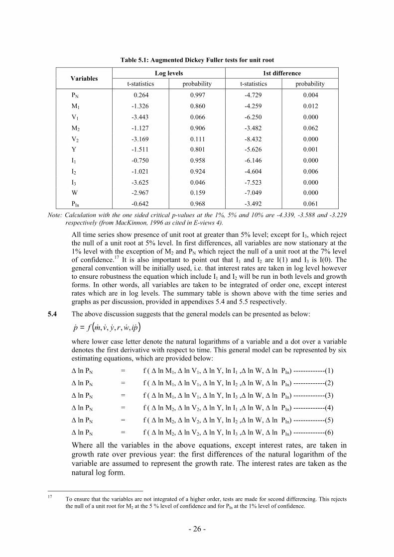
- 26 -

Table 5.1: Augmented Dickey Fuller tests for unit root

Variables Log levels 1st difference

t-statistics probability t-statistics probability

PN 0.264 0.997 -4.729 0.004 M1 -1.326 0.860 -4.259 0.012

V1 -3.443 0.066 -6.250 0.000 M2 -1.127 0.906 -3.482 0.062

V2 -3.169 0.111 -8.432 0.000 Y -1.511 0.801 -5.626 0.001

I1 -0.750 0.958 -6.146 0.000 I2 -1.021 0.924 -4.604 0.006 I3 -3.625 0.046 -7.523 0.000 W -2.967 0.159 -7.049 0.000 PIn -0.642 0.968 -3.492 0.061

Note: Calculation with the one sided critical p-values at the 1%, 5% and 10% are -4.339, -3.588 and -3.229 respectively (from MacKinnon, 1996 as cited in E-views 4).

All time series show presence of unit root at greater than 5% level; except for I3, which reject the null of a unit root at 5% level. In first differences, all variables are now stationary at the 1% level with the exception of M2 and PN which reject the null of a unit root at the 7% level of confidence.17 It is also important to point out that I1 and I2 are I(1) and I3 is I(0). The general convention will be initially used, i.e. that interest rates are taken in log level however to ensure robustness the equation which include I1 and I2 will be run in both levels and growth forms. In other words, all variables are taken to be integrated of order one, except interest rates which are in log levels. The summary table is shown above with the time series and graphs as per discussion, provided in appendixes 5.4 and 5.5 respectively.

5.4 The above discussion suggests that the general models can be presented as below:

( )piwryvmfp &&&&&& ,,,,,=

where lower case letter denote the natural logarithms of a variable and a dot over a variable denotes the first derivative with respect to time. This general model can be represented by six estimating equations, which are provided below:

∆ ln PN = f ( ∆ ln M1, ∆ ln V1, ∆ ln Y, ln I1 ,∆ ln W, ∆ ln PIn) -------------(1)

∆ ln PN = f ( ∆ ln M1, ∆ ln V1, ∆ ln Y, ln I2 ,∆ ln W, ∆ ln PIn) -------------(2)

∆ ln PN = f ( ∆ ln M1, ∆ ln V1, ∆ ln Y, ln I3 ,∆ ln W, ∆ ln PIn) -------------(3)

∆ ln PN = f ( ∆ ln M2, ∆ ln V2, ∆ ln Y, ln I1 ,∆ ln W, ∆ ln PIn) -------------(4)

∆ ln PN = f ( ∆ ln M2, ∆ ln V2, ∆ ln Y, ln I2 ,∆ ln W, ∆ ln PIn) -------------(5)

∆ ln PN = f ( ∆ ln M2, ∆ ln V2, ∆ ln Y, ln I3 ,∆ ln W, ∆ ln PIn) -------------(6)

Where all the variables in the above equations, except interest rates, are taken in growth rate over previous year: the first differences of the natural logarithm of the variable are assumed to represent the growth rate. The interest rates are taken as the natural log form.

17 To ensure that the variables are not integrated of a higher order, tests are made for second differencing. This rejects

the null of a unit root for M2 at the 5 % level of confidence and for PIn at the 1% level of confidence.

- 27 -

5.5 A simple ordinary least squares (OLS) estimation was used to assess the impact of the selected variables on Nepalese inflation. In the estimating equations, a structural break was found in 1989 utilizing the Chow break test, which was significant at the 1% level in all six representations. This result of a structural break in 1989 makes sense since it had marked the deregulation of domestic interest rates as well as was a precursor for economic liberalization in Nepal. The dummy variable 'DUMMY 1989'18 is thus included in the above-mentioned empirical estimations. The results of these six estimations and their respective associated coefficients are shown in tabular form in annex 5.7.

5.6 The results of the six regressions19, in general, explain over half of the regression; for M1 they are about 70% while for M2 they are about 62%, and have F-statistic suggests rejection of the null that all coefficients are jointly zero at greater than the 1% level of confidence.

Further, the Durbin Watson statistic rejects serial correlation at the 5% level of confidence. This suggests that no additional lag lengths are necessary as the present representation is able to address the problem of serial correlation. This result has to be taken into view of other studies which use high frequency data (such as Khan and Shimmelpfinnig (2006)). However their lag limits are of about one year - i.e. those adjustments, if any, take place within that period.20 Because of this and taken into view the annual frequency of the data, it is felt that there is no further necessity to lag the above-mentioned equations.

5.7 At this juncture, a process was initiated to identify the specific model. In this regard, Khan and Shimmelpfinnig (2006) had utilized a specialized computer routine which automatically tested down a general model. For the study the simpler methodology from Dlamini et al (2001) was utilized where variable deletion was based on confidence testing21 that the coefficient was not equal to zero. Based on this test, it was considered appropriate to exclude the insignificant variables. In this regard, looking at the variables of each equation, except for narrow money supply and Indian inflation, which are consistently significant, the remaining variables are not consistently significant at the 5% level of confidence and thus it was considered appropriate to exclude the insignificant variables.22 Of the remaining variable the money supply and Indian inflation are significant in all cases. Specifically for the money supply, M1 is utilized as the operational variable as it is significant at 5% level in contrast to a weaker performance of M2 (this conclusion is similar to many authors such as Khatiwada (1994), Maskay (1998), Nepal Rastra Bank, Monetary Division (2001) etc.). The model specific to Nepal is thus:

∆ ln PN = f ( ∆ ln M1, ∆ ln PIn)

5.8 This short-run estimation is provided as:

∆ ln PN = -0.03 + 0.18* ∆ ln M1 + 1.13* ∆ ln PIn

(-1.50) (1.92) (5.73)

The estimation explained 61 percent of the regression with the F-statistic being significant and the Durbin Watson statistic (2.36) rejecting the null of serial correlation. The estimation suggests that in the short-run Nepalese inflation reacts significantly to both growth of narrow

18 This was constructed with 0 from 1977/78 to 1988/89 and 1 from 1989/90 to 2005/2006. 19 The results did not significantly differ with I1 and I2 in level and growth forms. That is PIn is significant at more

than the 1% level in all cases, M1 at the 10% level in both cases while M2 in only one case, in another it was not significantly different to zero. The results are provided in Annex 5.8

20 Also, running the above six specification in the first lag produced mixed results in terms of the AIC statistic, shown in Annex 5.9.

21 This was based on Wald test with F-statistic and Chi-statistic; the p-value of the regression output gives the F-statistic of the Wald test.

22 The growth of broad money and growth of wages were consistently significant at the 10% level as well as the growth of wages, which also was consistently significant at the 10% level but for the later the coefficient had the opposite expected theoretical sign.

- 28 -

money supply and Indian inflation, although the reaction of Nepalese inflation to money supply growth is only a fraction of that to Indian inflation.23

5.9 Engle and Granger (1987) pointed out that a linear combination of two or more non-stationary series may be stationary. If such stationary, or I (0) or linear combination exists, the non-stationary series are said to be cointegrated; therefore, this analysis tests whether the linear combinations of the non-stationary series of same order of integration, is stationary. If there is some tendency for some linear relationships to hold among a set of variables over a long period of time, the cointegration analysis will help to discover it. The stationary linear combination is called the cointegrating equation and is interpreted as the long-run equilibrium relationship between the variables. Cointegration will allow us to include a combination of long and short run information in the same model. This helps us to cover some drawbacks associated with the loss of long-run information from simple attempts to achieve a stationary series through differencing. Running the Johansen method for testing if cointegration exists in all three variable results in:

Table 5.2: Cointegration results

Hypothesized Trace 5% 1% Max-Eigen 5% 1% No. of CE(s) Eigenvalue Statistic Critical

Value Critical Value

Statistic Critical Value

Critical Value

None * 0.513358 33.09301 29.68 35.65 19.44613 20.97 25.52 At most 1 0.364307 13.64688 15.41 20.04 12.23206 14.07 18.63 At most 2 0.051051 1.414819 3.76 6.65 1.414819 3.76 6.65

The trace statistic suggests that there is presence of 1 cointegrating equation at the 5% level while the Max-Eigen statistic suggests a similar conclusion but at the 6% level. Having determined the presence of one cointegrating equation among the three variables;24 the long-term cointegrating equation is given as:

ln PN = -0.62 + 0.07* ln M1 + 0.96* ln PIn

(-3.51) (0.78) (5.63)

The t-statistics in parenthesis suggest that the money supply is not part of the long-run relationship. Dropping this term is consistent with Khan and Shimmelpfinnig (2006), which will also provide additional degrees of freedom. This final relationship suggests that the only remaining factor influencing Nepalese price levels is the Indian price level. Estimating this representation results in:

ln PN = -0.49 + 1.09* ln PIn

(-9.98) (95.25)

Based in the above suggests that, Nepalese price level is significantly influenced by Indian price level. The coefficient suggests that Nepalese price levels are more reactive to Indian price; a 1 percent increase in Indian price level is reflected in a 1.09 percent increase in Nepalese price levels.

5.10 To investigate the short-run dynamics, estimation of the error-correction model (ECM) is undergone. The distinctive feature of ECM is that the long-run equilibrium position is not embodied explicitly but its effect is captured by the Error Correction (EC) term. This is formulated as:

23 Broad money was also used however an insignificant coefficient resulted although maintaining the significant

relation with Indian inflation. 24 This conclusion is supported by testing the error terms for unit root. The null hypothesis of a unit root is rejected at

more than the 1% level of confidence (ADF statistic -6.141592 p-value 0.0001 Critical value at 1% level is -4.339330).

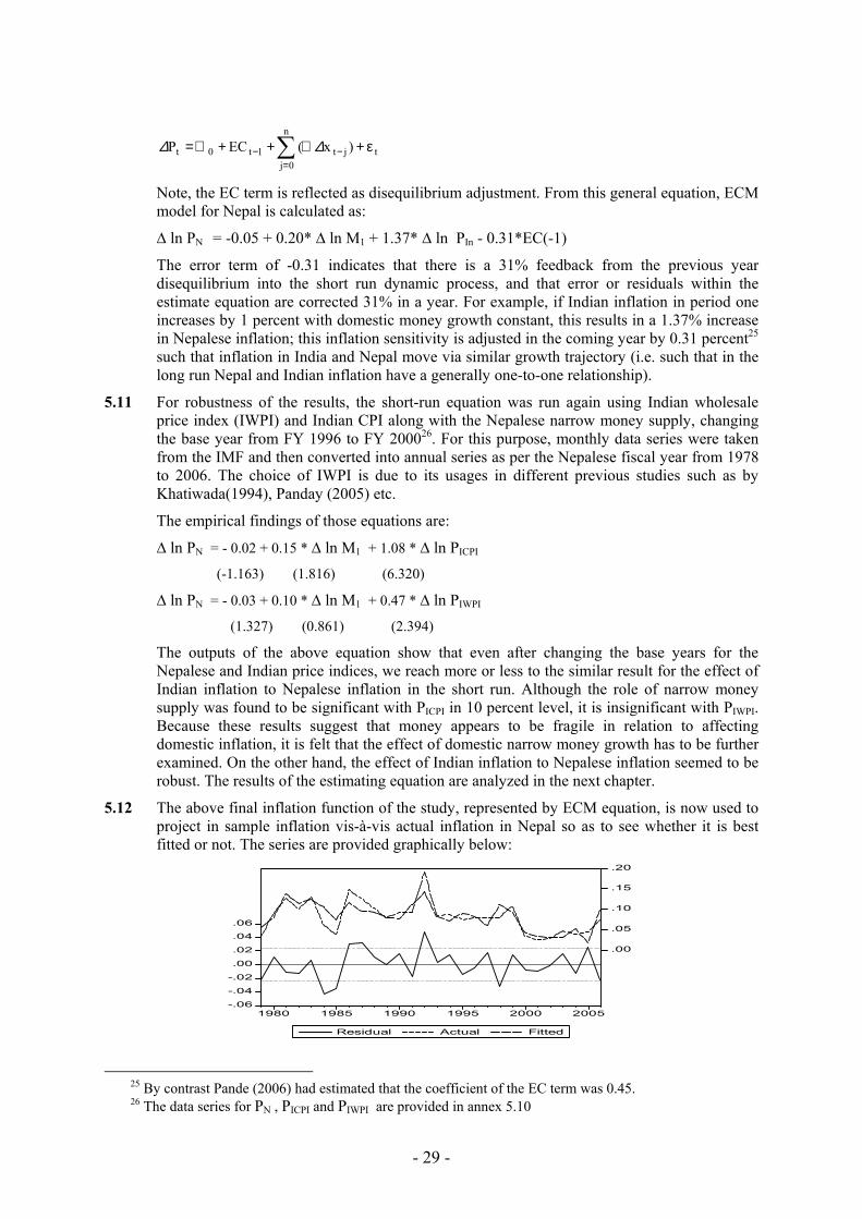
- 29 -

∑=

−− ε+℘++℘=n

0jtjt1t0t )x(ECP ∆∆

Note, the EC term is reflected as disequilibrium adjustment. From this general equation, ECM model for Nepal is calculated as:

∆ ln PN = -0.05 + 0.20* ∆ ln M1 + 1.37* ∆ ln PIn - 0.31*EC(-1)

The error term of -0.31 indicates that there is a 31% feedback from the previous year disequilibrium into the short run dynamic process, and that error or residuals within the estimate equation are corrected 31% in a year. For example, if Indian inflation in period one increases by 1 percent with domestic money growth constant, this results in a 1.37% increase in Nepalese inflation; this inflation sensitivity is adjusted in the coming year by 0.31 percent25 such that inflation in India and Nepal move via similar growth trajectory (i.e. such that in the long run Nepal and Indian inflation have a generally one-to-one relationship).

5.11 For robustness of the results, the short-run equation was run again using Indian wholesale price index (IWPI) and Indian CPI along with the Nepalese narrow money supply, changing the base year from FY 1996 to FY 200026. For this purpose, monthly data series were taken from the IMF and then converted into annual series as per the Nepalese fiscal year from 1978 to 2006. The choice of IWPI is due to its usages in different previous studies such as by Khatiwada(1994), Panday (2005) etc.

The empirical findings of those equations are:

∆ ln PN = - 0.02 + 0.15 * ∆ ln M1 + 1.08 * ∆ ln PICPI

(-1.163) (1.816) (6.320)

∆ ln PN = - 0.03 + 0.10 * ∆ ln M1 + 0.47 * ∆ ln PIWPI

(1.327) (0.861) (2.394)

The outputs of the above equation show that even after changing the base years for the Nepalese and Indian price indices, we reach more or less to the similar result for the effect of Indian inflation to Nepalese inflation in the short run. Although the role of narrow money supply was found to be significant with PICPI in 10 percent level, it is insignificant with PIWPI. Because these results suggest that money appears to be fragile in relation to affecting domestic inflation, it is felt that the effect of domestic narrow money growth has to be further examined. On the other hand, the effect of Indian inflation to Nepalese inflation seemed to be robust. The results of the estimating equation are analyzed in the next chapter.

5.12 The above final inflation function of the study, represented by ECM equation, is now used to project in sample inflation vis-à-vis actual inflation in Nepal so as to see whether it is best fitted or not. The series are provided graphically below:

-.06

-.04

-.02

.00

.02

.04

.06

.00

.05

.10

.15

.20

1980 1985 1990 1995 2000 2005

Residual Actual Fitted

25 By contrast Pande (2006) had estimated that the coefficient of the EC term was 0.45. 26 The data series for PN , PICPI and PIWPI are provided in annex 5.10

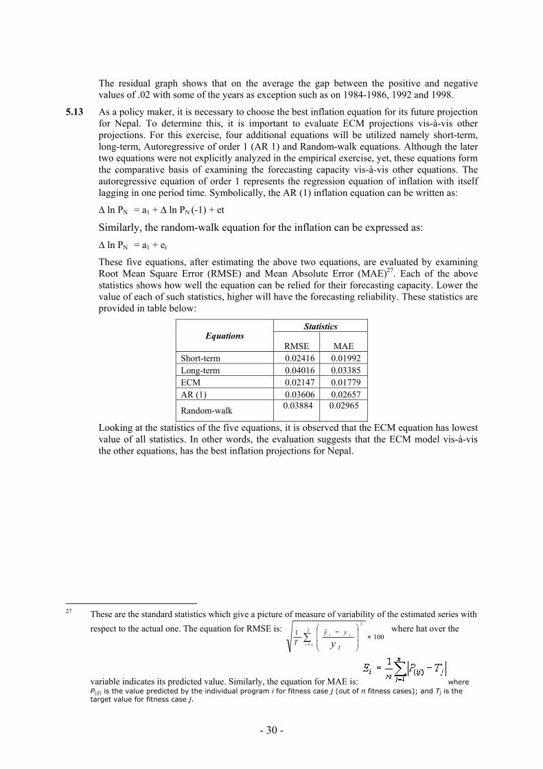
- 30 -

The residual graph shows that on the average the gap between the positive and negative values of .02 with some of the years as exception such as on 1984-1986, 1992 and 1998.

5.13 As a policy maker, it is necessary to choose the best inflation equation for its future projection for Nepal. To determine this, it is important to evaluate ECM projections vis-à-vis other projections. For this exercise, four additional equations will be utilized namely short-term, long-term, Autoregressive of order 1 (AR 1) and Random-walk equations. Although the later two equations were not explicitly analyzed in the empirical exercise, yet, these equations form the comparative basis of examining the forecasting capacity vis-à-vis other equations. The autoregressive equation of order 1 represents the regression equation of inflation with itself lagging in one period time. Symbolically, the AR (1) inflation equation can be written as:

∆ ln PN = a1 + ∆ ln PN (-1) + et

Similarly, the random-walk equation for the inflation can be expressed as: ∆ ln PN = a1 + et

These five equations, after estimating the above two equations, are evaluated by examining Root Mean Square Error (RMSE) and Mean Absolute Error (MAE)27. Each of the above statistics shows how well the equation can be relied for their forecasting capacity. Lower the value of each of such statistics, higher will have the forecasting reliability. These statistics are provided in table below:

Equations

Statistics

RMSE MAE Short-term 0.02416 0.01992 Long-term 0.04016 0.03385 ECM 0.02147 0.01779 AR (1) 0.03606 0.02657

Random-walk 0.03884

0.02965

Looking at the statistics of the five equations, it is observed that the ECM equation has lowest value of all statistics. In other words, the evaluation suggests that the ECM model vis-à-vis the other equations, has the best inflation projections for Nepal.

27 These are the standard statistics which give a picture of measure of variability of the estimated series with

respect to the actual one. The equation for RMSE is: 100

ˆ12

1×

−∑

=

T

t

tt

t

yyT y

where hat over the

variable indicates its predicted value. Similarly, the equation for MAE is: where P(ij) is the value predicted by the individual program i for fitness case j (out of n fitness cases); and Tj is the target value for fitness case j.

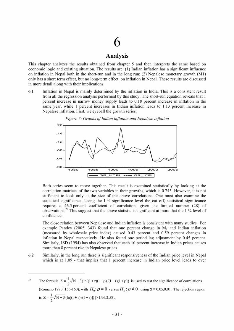
- 31 -

6 Analysis

This chapter analyzes the results obtained from chapter 5 and then interprets the same based on economic logic and existing situation. The results are: (1) Indian inflation has a significant influence on inflation in Nepal both in the short-run and in the long run; (2) Nepalese monetary growth (M1) only has a short term effect, but no long-term effect, on inflation in Nepal. These results are discussed in more detail along with their implications.

6.1 Inflation in Nepal is mainly determined by the inflation in India. This is a consistent result from all the regression analysis performed by this study. The short-run equation reveals that 1 percent increase in narrow money supply leads to 0.18 percent increase in inflation in the same year, while 1 percent increases in Indian inflation leads to 1.13 percent increase in Nepalese inflation. First, we eyeball the growth series:

Figure 7: Graphs of Indian inflation and Nepalese inflation

.00

.04

.08

.12

.16

.20

1980 1985 1990 1995 2000 2005

GR_NCPI GR_ICPI

Both series seem to move together. This result is examined statistically by looking at the

correlation matrices of the two variables in their growths, which is 0.745. However, it is not sufficient to look only at the size of the above correlations. One must also examine the statistical significance. Using the 1 % significance level the cut off, statistical significance requires a 46.5 percent coefficient of correlation, given the limited number (28) of observations.28 This suggest that the above statistic is significant at more that the 1 % level of confidence.

The close relation between Nepalese and Indian inflation is consistent with many studies. For example Pandey (2005: 343) found that one percent change in M1 and Indian inflation (measured by wholesale price index) caused 0.43 percent and 0.59 percent changes in inflation in Nepal respectively. He also found one period lag adjustment by 0.45 percent. Similarly, ISD (1994) has also observed that each 10 percent increase in Indian prices causes more than 8 percent rise in Nepalese prices.

6.2 Similarly, in the long run there is significant responsiveness of the Indian price level in Nepal which is at 1.09 - that implies that 1 percent increase in Indian price level leads to over

28 The formula ]}1)(r1/()1)(r1{ln[(3N

21Z ρ+−ρ−+−= is used to test the significance of correlations

(Romano 1970: 156-160), with H0 0:ρ = versus H A:ρ ≠ 0 , using 01.0,05.0=α . The rejection region

is 58.2,96.1|)]}r1/()r1{ln[(3N21|Z >−+−= .

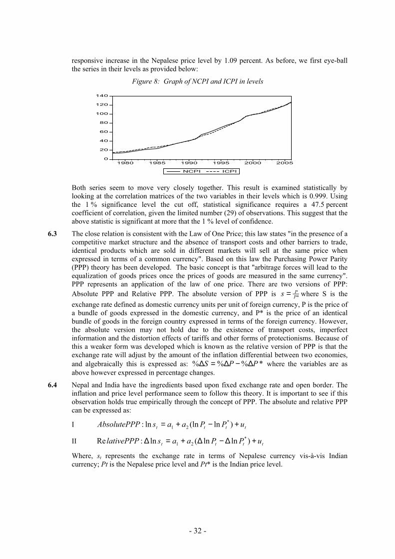
- 32 -

responsive increase in the Nepalese price level by 1.09 percent. As before, we first eye-ball the series in their levels as provided below:

Figure 8: Graph of NCPI and ICPI in levels

0

20

40

60

80

100

120

140

1980 1985 1990 1995 2000 2005

NCPI ICPI

Both series seem to move very closely together. This result is examined statistically by

looking at the correlation matrices of the two variables in their levels which is 0.999. Using the 1 % significance level the cut off, statistical significance requires a 47.5 percent coefficient of correlation, given the limited number (29) of observations. This suggest that the above statistic is significant at more that the 1 % level of confidence.

6.3 The close relation is consistent with the Law of One Price; this law states "in the presence of a competitive market structure and the absence of transport costs and other barriers to trade, identical products which are sold in different markets will sell at the same price when expressed in terms of a common currency". Based on this law the Purchasing Power Parity (PPP) theory has been developed. The basic concept is that "arbitrage forces will lead to the equalization of goods prices once the prices of goods are measured in the same currency". PPP represents an application of the law of one price. There are two versions of PPP: Absolute PPP and Relative PPP. The absolute version of PPP is *P

Ps = where S is the exchange rate defined as domestic currency units per unit of foreign currency, P is the price of a bundle of goods expressed in the domestic currency, and P* is the price of an identical bundle of goods in the foreign country expressed in terms of the foreign currency. However, the absolute version may not hold due to the existence of transport costs, imperfect information and the distortion effects of tariffs and other forms of protectionisms. Because of this a weaker form was developed which is known as the relative version of PPP is that the exchange rate will adjust by the amount of the inflation differential between two economies, and algebraically this is expressed as: *%%% PPS ∆−∆=∆ where the variables are as above however expressed in percentage changes.

6.4 Nepal and India have the ingredients based upon fixed exchange rate and open border. The inflation and price level performance seem to follow this theory. It is important to see if this observation holds true empirically through the concept of PPP. The absolute and relative PPP can be expressed as:

I tttt uPPaasPAbsolutePP +−+= )ln(lnln: *21

II tttt uPPaaslativePPP +∆−∆+=∆ )lnln(ln:Re *21

Where, st represents the exchange rate in terms of Nepalese currency vis-à-vis Indian currency; Pt is the Nepalese price level and Pt* is the Indian price level.

- 33 -

For absolute PPP to hold, the regression estimates would yield a1 = ln(st) and a2=0. We test the equation I and II using the quarterly data29 from FY 1995 to 2006; since in 1994 (FY 1995) the last adjustment had been made in exchange rate that was fixed as Nepalese Rs 1.6 per Indian Rupees. Running the equation I we obtain:

)ln(ln*00.047.0ln *ttt PPs −+=

p-value (0.0000) (0.0573)

The above result shows that absolute PPP has a good hold in case of Nepal and India over the period of 1995 to 2006, since the coefficient of a1 is equal to natural logarithm of the exchange rate, 1.6, which is significant at 10 percent level, and the coefficient of a2 is not significant from zero.

For relative PPP to hold, the regression estimates would yield a1=0 and a2=1. Since exchange rate is fixed at 1.6 over the period, the left hand side of the above equation (growth of st) will be zero and hence re-arranging the equation II, we get relative PPP as:

tt uPaaP +∆+=∆ *21 lnln

Running this equation, we get the output as:

tt uPP +∆+−=∆ *ln18.1004.0ln

p-value (0.3077) (0.000)

We found the estimate of a1 not significant from zero and that of a2 to be 1.18 which was significant at 1 percent level. The result suggests that relative PPP has also a good hold from FY 1994 to 2006 on quarterly time series. We thus can conclude from the above two PPP theories that because of the arbitrages between the goods and services the prices in India are similar to that of Nepal at the existing exchange rate system.

6.5 The empirical results from the error correction equation suggest that after each period there is a 31 percent adjustment to correct for the over-shooting of Nepalese inflation. It is hypothesized that adjustment in prices takes place through the channel of the Balance of Payments (BOP) via goods arbitrage. That is, if the same good is priced differently in adjacent markets there is an incentive to export the good from the cheaper market and sell it in the expensive market. Such profit-motivated activity tends to equalize the prices in both markets. This gives an explanation to the close relationship between Nepalease and Indian prices and inflation. Because of the open-border between Nepal and India, any price differentials in the products attract people to go for goods arbitrage that do not account in the BOP. The volume of such arbitrages is high in border regions. The process continues to occur till there is no incentive for further arbitrage that is prices come to be equalized. This can be seen in the close association of border prices of some selected commodities (annex 6.2), collected by the Nepal Rastra Bank's officials from the nearby offices.

The BOP channel can be seen in the high level of trade between Nepal and India. However, this figure underestimates the true level of trade. This is because of the high level of unrecorded trade (i.e. being border trade and illegal trade). There are different estimates for the level of informal trade between both countries. For example, Karmacharya et al. (2004) suggested that this figure is about 40%, which is consistent with similar studies, such as by Nepal Rastra Bank.

6.6 The empirical result, which suggests that monetary growth, does not have a long-term impact on inflation in Nepal, is surprising, taking into consideration the statement that inflation in the long run is everywhere a monetary phenomenon. However, this conclusion is limited to a

29 The data series are provided in the annex 6.1 which are calculated by the author from the monthly data series taken

from IMF.

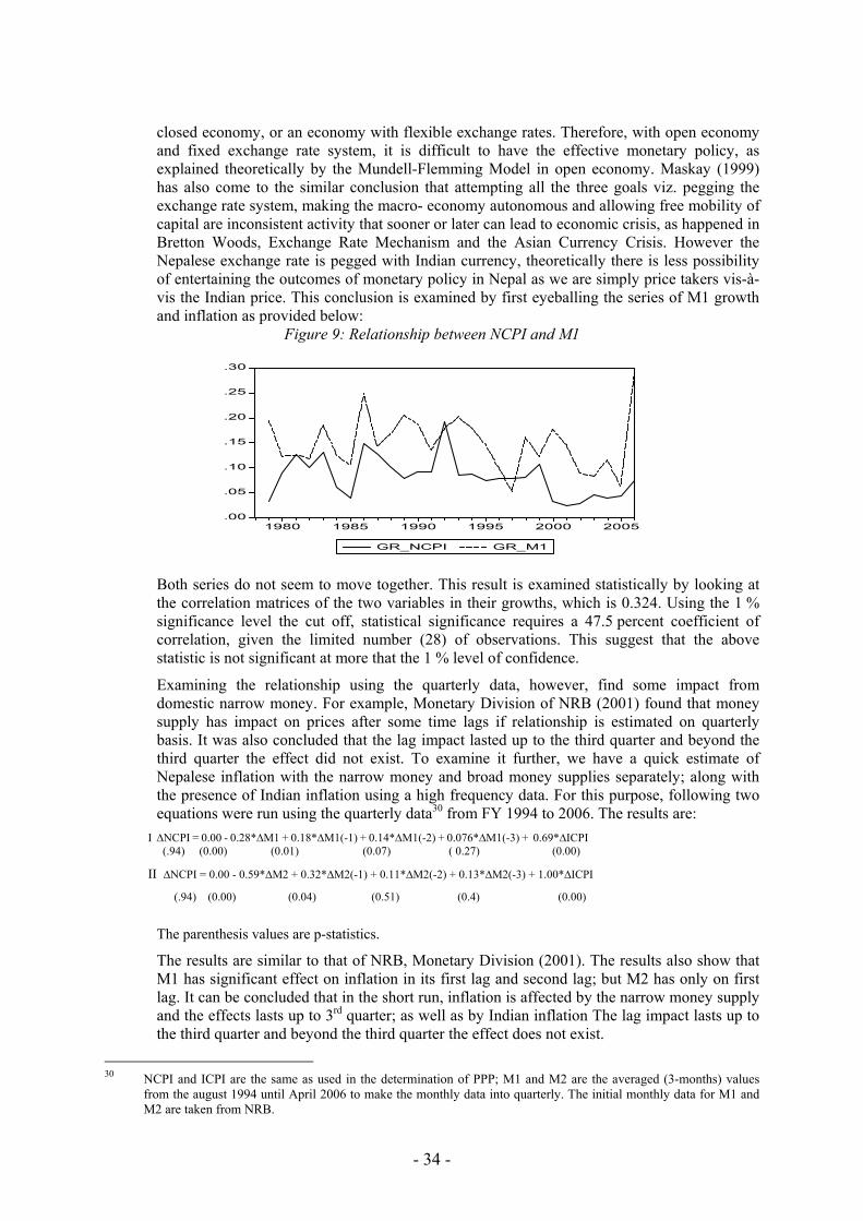
- 34 -

closed economy, or an economy with flexible exchange rates. Therefore, with open economy and fixed exchange rate system, it is difficult to have the effective monetary policy, as explained theoretically by the Mundell-Flemming Model in open economy. Maskay (1999) has also come to the similar conclusion that attempting all the three goals viz. pegging the exchange rate system, making the macro- economy autonomous and allowing free mobility of capital are inconsistent activity that sooner or later can lead to economic crisis, as happened in Bretton Woods, Exchange Rate Mechanism and the Asian Currency Crisis. However the Nepalese exchange rate is pegged with Indian currency, theoretically there is less possibility of entertaining the outcomes of monetary policy in Nepal as we are simply price takers vis-à-vis the Indian price. This conclusion is examined by first eyeballing the series of M1 growth and inflation as provided below:

Figure 9: Relationship between NCPI and M1

.00

.05

.10

.15

.20

.25

.30

1980 1985 1990 1995 2000 2005

GR_NCPI GR_M1

Both series do not seem to move together. This result is examined statistically by looking at

the correlation matrices of the two variables in their growths, which is 0.324. Using the 1 % significance level the cut off, statistical significance requires a 47.5 percent coefficient of correlation, given the limited number (28) of observations. This suggest that the above statistic is not significant at more that the 1 % level of confidence.

Examining the relationship using the quarterly data, however, find some impact from domestic narrow money. For example, Monetary Division of NRB (2001) found that money supply has impact on prices after some time lags if relationship is estimated on quarterly basis. It was also concluded that the lag impact lasted up to the third quarter and beyond the third quarter the effect did not exist. To examine it further, we have a quick estimate of Nepalese inflation with the narrow money and broad money supplies separately; along with the presence of Indian inflation using a high frequency data. For this purpose, following two equations were run using the quarterly data30 from FY 1994 to 2006. The results are:

I ∆NCPI = 0.00 - 0.28*∆M1 + 0.18*∆M1(-1) + 0.14*∆M1(-2) + 0.076*∆M1(-3) + 0.69*∆ICPI (.94) (0.00) (0.01) (0.07) ( 0.27) (0.00) II ∆NCPI = 0.00 - 0.59*∆M2 + 0.32*∆M2(-1) + 0.11*∆M2(-2) + 0.13*∆M2(-3) + 1.00*∆ICPI

(.94) (0.00) (0.04) (0.51) (0.4) (0.00)

The parenthesis values are p-statistics.

The results are similar to that of NRB, Monetary Division (2001). The results also show that M1 has significant effect on inflation in its first lag and second lag; but M2 has only on first lag. It can be concluded that in the short run, inflation is affected by the narrow money supply and the effects lasts up to 3rd quarter; as well as by Indian inflation The lag impact lasts up to the third quarter and beyond the third quarter the effect does not exist.

30 NCPI and ICPI are the same as used in the determination of PPP; M1 and M2 are the averaged (3-months) values

from the august 1994 until April 2006 to make the monthly data into quarterly. The initial monthly data for M1 and M2 are taken from NRB.

- 35 -

6.7 There are three implications of the above results.

• First, in regard to regulated prices. Because of the open border, any price differential in the regulated product can favor the informal trade towards the high pricing country from low pricing country. As a result, there is high chance of inflation to be equalized via arbitrages of goods and services towards low pricing country. For example the open border between Nepal and India with the present low price of regulated product in Nepal compared to India favors arbitrage speculation toward Indian market and hence any subsidy given to such products in Nepal will benefit to Indian consumers and vice-versa. This is elaborated in the box below for petroleum products.

Box 3: Example of arbitrage with petroleum products The article 'Subsidy on fuel price costs people dearly' published in the Kathmandu Post daily dated 10 January, 2007 also shows that the arbitrages of such products are common in the cross-border areas. Mr. Milan Mani Sharma quoting the study of Nepal Planning Commission has expressed that such an arbitrage has made the benefits to the Indian people rather than to Nepalese. Quoting to the high level studies of the government, the article says that about 25 percent of the oil-price subsidy goes to India every year. This reflects that even if there is legal control for such an unofficial trade, people are not stopped to do so and hence any price differentials on the products between the two countries are likely to encourage the trade speculators. There are three ways to stop them: i) to close the border ii) to adjust the exchange rate as per the theory of PPP and iii) to adjust the local price consistent with the prices in Indian market in the existing system of fixed exchange rate. The first two options are likely to create many implications. In such a situation, the only way to settle down the problem of arbitrages is to adjust the domestic price to be consistent with the prices of Indian products.

Source: http://www.kantipuronline.com/kolnews.php?&nid=97090, 10 January, 2007

• Second, the low level of capital mobility in the short-run appears to allow some independence of domestic monetary policy. Activities to increase the level of capital mobility (such as for greater capital account convertibility) will shrink the window for having domestic monetary policy. In the short-run, there is limited capital mobility because the agents are not much informed within short period of time about any implications of the policy changes like interest rate differential, price differential etc. perhaps due to policy noise or lack of technological avenues. It will take time to adjust their decision according to the policy changes. As a result during this period there is significant effect of monetary policy to influence the inflation in domestic economy. Whereas in the long run people have much time to adjust their decision as per the policy changes.31

• Third is in regard to having an inflation target by Nepal. Since inflation in Nepal is significantly influenced by Indian inflation, having an inflation target within the present domestic context requires to make more vigorous exercise especially in the context of present arrangement that suggests Nepal has been importing the favorable inflation performance of India. This can also be seen in the monetary policy statements for continuation of the pegged exchange rate regime with Indian currency.

31 This result of variable capital mobility is explained in the textbook (D. Joseph and V. David 1999).

- 36 -

7 Conclusions and Recommendations

7.1 The study began with the premise that it is essential for the Nepal Rastra Bank to be aware of the major determinants of inflation in Nepal, for meeting the objective of domestic price stability. In this regard, it is felt that the study has achieved this main objective. This was achieved by the study initially looking at a hybrid model of inflation - e.g. open economy monetary model with structural factors - which had incorporated demand pull and cost push (via imported price) theories of inflation. From this general model a specific model of inflation was developed for Nepal which was subject to a battery of empirical exercises namely cointegration technique and error correction modeling (ECM).

7.2 Empirical results suggest that inflation in Nepal is mainly determined by Indian inflation with narrow money only having an effect in the short run (less than one year). The study attributed this result to the geographical situation of having a shared open and contiguous border, which facilitates informal trade and goods arbitrage, a rigid pegged exchange rate regime between both currencies along with time varying capital mobility: i.e. it is less mobile in the short term (less than one year) but being more so in the long term. The study had therefore concluded that within the existing framework of pegged exchange rate and capital mobility, the main influencing factor of inflation is from India with the NRB having control over domestic inflation only in the short run (a one year window) but limited control beyond that.

7.3 The above results are similar with many other studies which suggest that inflation in India is an important contributor for inflation in Nepal. For example, Thapa (2004) had stated, “…so long as Nepal maintains fixed exchange rate regime with India, inflation cannot be the monetary policy objective”. However, there has been discussion on the magnitude of influence. This study suggests that there is a near unity relationship, which is corroborated with holding of absolute and relative purchasing power parity. This result is also similar to IMF (1993), which has concluded that Nepal’s inflation is basically determined by Indian inflation. In the words of IMF, “When Nepal’s CPI is regressed on India’s WPI corrected for the exchange rate, the coefficient on India’s price level is very close to 1”.

7.4 Given this conclusion, the study makes three recommendations:

• First, to establish a mechanism to continuously monitor price developments in India to ensure harmonization of domestic regulated prices (e.g. petroleum products etc.). This is because with significant differences in the regulated prices between India and Nepal, high level of arbitrages in border areas becomes common practices and thereby affecting Nepalese inflation.

• Second, to commence studies for examining the implication of increasing the level of capital mobility between both countries. Indian has already indicated for having greater degree of capital convertibility in their 2006 report by the Tarapore Commission. Such activities will likely have to be followed by Nepal. A greater degree of capital convertibility will result in higher level of capital flow between both countries. Given the existing rigid exchange rate, this make the window for the Nepal Rastra Bank to influence inflation smaller. Further, there is an important implication on the exchange rate policy currently followed by the country. While outside the scope of the study, it is important to be proactive about the effects this will have.

• Third, to refine monetary policy formulation based on the above results. Presently, monetary policy is geared toward maintenance of price stability. However, the empirical exercise of the bank suggests that the main contributor for inflation in the country is from India. This has implication and suggests that NRB should rethink

- 37 -

before commencing activities for having an inflation-targeting framework. Also and given that the exchange rate policy is maintained, it is important to refine monetary formulation in this regard.

Box 4: Inflation-targeting and Nepal32

Background on Inflation Targeting: Inflation Targeting (IT) refers to the quantitative announcement of inflation by the monetary authority to keep it within a point, or range of points for the next period of time. Central Banks, as a monetary authority, have been searching for an appropriate nominal anchor for monetary policy ever since the early 1970s with breakdown of the Bretton Woods system of fixed but adjustable exchange rates. This period saw many countries pursue greater flexibility in their exchange rates to allow more responsiveness and flexibility to market forces. In the early 1990s, the Reserve Bank of New Zealand was the first central bank that formally introduced IT regime as an alternative nominal anchor for monetary policy under flexible exchange rate. Presently, there are 23 countries that have adopted IT as a stance of monetary policy; and there is increasing tendency of getting technical assistance33 by International Monetary Fund (IMF) by the member countries for the introduction of IT in their countries (IMF 2006). The spread of inflation targeting at present days has coincided with a period of low and stable inflation and well-anchored inflation expectation in the world, although the biggest monetary systems such as USA and Euro area are not explicitly undergone to IT. This is one of the reasons why the central banks are pleaded with IT as a stance of monetary policy. Also, inflation target is readily understood by the public and is thus highly transparent to them than monetary targets. If the relationship between monetary aggregates and the inflation goal variable is subject to unpredictable shifts, as has occurred in many countries such as Switzerland, then monetary targets lose their transparency because they are no longer able to accurately signal the stance of monetary policy.

Arrangements to Facilitate Functioning of Inflation-Targeting Regime: An effective IT regime will benefit the economy by limiting inflation distortions and anchoring inflation expectations by making the central bank more credible and accountable to the public.

There are some conditions to be satisfied for the success of an IT regime, namely: • There should be clear-cut legal mandate to the central bank to pursue price stability (or low inflation) as the core

objective of monetary policy. • The central bank should be given sufficient autonomy to set operational targets without government or political

interference. • Central banks should have adequate ability to influence inflation through its policy instruments. • There should exist well-coordinated monetary and fiscal operations. • There should exist a reasonably stable and well-developed financial system. • There should exist sound methodology to monitor economy and forecast inflation. • There should exist a transparency mechanism and communications strategy, to build credibility and accountability of

the Central Bank.

Inflation Targeting and Nepal: Presently Nepal targets the money supply (M1 and M2) under a monetary targeting framework. The choice of this framework is due to a stable demand for money function (in relation to income and prices) in the country with limited financial sector development. Since 1960, Nepal has been following a de facto fixed exchange rate with Indian currency. The choice of this exchange rate policy is due mainly to geographical proximity, large trade share and open, porous border with India. Such an exchange rate mechanism potentially undermines the effectiveness of the monetary policy. This has resulted in Nepalese inflation being highly influenced by such movements in India. As such and with the present fixed exchange rate, it is felt that an IT framework for Nepal may not make sense at this time. However the future is dynamic with the domestic and international environment every changing, it is thus important to continuously evaluate the situation for IT. Thus a comprehensive study in this regard, is essential to keep abreast of the evolving IT situation.

7.5 The study ends with a closing observation that the study simply describes the relationship. This observation is important since it gives information for having the appropriate policy action for achieving domestic financial stability in the country. While the analysis and observation is open to debate, it is important that this is to be addressed proactively. In this way, the study team feels that the activities of the Nepal Rastra Bank will be made much stronger.

32 The above discussion is based on the notes made courteously available by Deputy Director Mr. Shaligram Dahal during

his attendance in the Workshop on Inflation Targeting and Macro modeling jointly organized by the IMF and the Bank of Thailand in Chiang Mai, Thailand on 6 - 13 November 2006.

33 Inflation Targeting and the IMF, International Monetary Fund, March 2006.

- 38 -

References Barro, Robert J. (1996), Inflation and Growth, Federal Reserve Bank of St. Louis: Review

Batini, Nicoletta, and Anthony Yates (2003), Hybrid Inflation and Price-Level Targeting, Journal of Money, Credit and Banking, Vol. 35 (June), pp. 283–300 (as cited in World Economic Outlook April 2006: pp.161)

Bernanke, Ben S. (2006), The Benefits of Price Stability, BIS Review 13, www.bis.org

Blavy, Rodolphe (2004), Inflation and Monetary Pass-Through in Guinea, IMF Working Paper WP/04/223 Washington: International Monetary Fund

Bohara, Alok K. and Robert F. McNown (1989), Monetary and Inflationary Linkages between India and Nepal: A Vector Autoregression Analysis, The Indian Economic Journal. Vol. 37, No. 1, pp. 40 - 55.

Cagan, P. (1956), The Monetary Dynamics of Hyperinflation, in Friedman, M. (ed.), Studies in the Quantity Theory of Money, Chicago: University of Chicago Press, 25–117

Campillo, Marta and Jeffrey A. Miron (1996), Why does Inflation Differ Across Countries? NBER Working Paper No. 5540 Cambridge: National Bureau of Economic Research, MA

De Brouwer, Gordon and Neil R. Ericsson (1995), Modeling Inflation in Australia, research Discussion Paper 9510, Economic Analysis and Economic Research Department Reserve Bank of Australia

Dlamini, Acute, Armstrong Dlamini and Tsidi Nxumalo (2001), A Cointegration Analysis of the Determinants of Inflation in Swaziland, www.centralbank.org.sz/docs/Inflation. Paper.pdf

Domac, Ilker (2004), Explaining and Forecasting Inflation in Turkey, Policy Research Working Paper-WPS 3287, The World Bank,

Domac, Ilker and Carlos Elbirt (1998), The Main Determinants of Inflation in Albania, Policy Working Paper - WPS 1930, World Bank

Enders, Walter (2003), Applied Econometric Time Series, Second Edition, Tohn Wiley & Sons (Asia) Pvt. Ltd.

Ferguson, R. W. (2005), Speech delivered at the Cato Institute 23rd Annual Monetary Conference on Monetary Institutions and Economic Development, http://www.federalreserve.gov/BoardDocs/speeches/2005/20051103/default.htm

Friedman, Milton (1977), Inflation and Unemployment, Journal of Political Economy, Vol. 85 (3), p.451-72

Fry, M. J. (1974), Resource Mobilization and Financial Development in Nepal, Kathmandu: CEDA and Nepal Rastra Bank

Gujarati, Damodar N. (2004), Basic Econometrics, 4th edition. Tata McGraw-Hill,Publishing Co. Ltd, New Dellhi

H. White (1980), Econometrica, Vol. 48, No 3. URL: http://citeseer.ist.psu.edu/update/557535

Institute for Sustainable Development (1994), Inflation in Nepal, Economic Review Kathmandu: Nepal Rastra Bank Occasional Paper No.7 pp. 99 - 108

International Monetary Fund (1993), Nepal, IMF Economic Reviews, No. 13, pp 9-11.

Jacqueline Dwyer and Kenneth Leong (2001), Changes in the Determinants of Inflation in Australia, Research Discussion Paper 2001 - 02. Economic Group, Reserve Bank of Australia

Karmacharya, Binod Kumar (2004), India’s Informal Trade in SAARC Countries: Case of Nepal, India and Sri Lanka, (with N. Taneja and S. Sarvanathan), South Asia Economic Journal, Vol. 5, No. 1, Jan-June, pp. 27-54.

Keynes, John Maynard (1940), How to Pay for the War, London: Macmillan.

Khan, Mohsin S. and Schimmelpfennig, Axel (2006), Inflation in Pakistan: Money or Wheat? IMF Working Paper No. 06/60 Available at SSRN.

Khatiwada, Yuba Raj (1981), An Econometric Analysis of the Determinants of Inflation in Nepal, Economic Instruction Committee, Kirtipur Campus, Tribhuvan University, Kathmandu.

- 39 -

Khatiwada, Yuba Raj (1994), Some Aspects of Monetary Policy in Nepal, New Delhi: South Asian Publishers.

Kibritçioğlu, A. (2002), Causes of Inflation in Turkey: A Literature Survey with Special Reference to Theories of Inflation, in Inflation and Disinflation in Turkey, ed. by Kibritçioğlu, A., L. Rittenberg, and F. Selçuk, Aldershot: Ashgate, pp. 43-76

King, R. G. (2000), The New IS-LM Model: Language, Logic, and Limits, Federal Reserve Bank of Richmond, Economic Quarterly, 86 (3): 45–103.

Lissovolik, Bogdan (2003), Determinants of Inflation in a Transition Economy: The Case of Ukraine IMF Working Paper WP/03/126 International Monetary Fund

MacKinnon, James G. (1996), Numerical Distribution Functions for Unit Root and Cointegration Tests, Journal of Applied Econometrics, 11, 601-618.

Maliszewski, Wojciech (2003), Modeling Inflation in Georgia, IMF Working Paper WP/03/212. International Monetary Fund

Mankiw, N. G. (1985), Small Menu Costs and Large Business Cycles: A Macroeconomic Model for Monopoly, Quarterly Journal of Economics, 100 (2): 529–38

Maskay, Nephil Matangi (1998), The Impact of the Indian Monetary Policy and the Official Exchange Rate on Nepalese Monetary Policy, Economic Review, Nepal Rastra Bank, Occasional Paper, Number 10 -Pp 44 - 63.

Maskay, Nephil Matangi (1999), Addressing the ‘Unholy’ Trinity in Nepal-India Monetary Relations; Lessons from Bretton Woods, the Exchange Rate Mechanism and the Present Asian Currency Crisis, Economic Journal of Nepal, Vol. 22, No. 3. (July - Sept. 1999) 103 - 155.

Maskay, Nephil Matangi. (2000), Of Monetary Policy Analysis and Output Shocks, Economic Review Kathmandu: Nepal Rastra Bank Occasional Paper No. 12 pp. 17 - 28.

Mathema, Shushil Ram (1998), Determinants of Inflation with Special Reference to Wages in Nepal, Economic Review Kathmandu: Nepal Rastra Bank Occasional Paper No. 10 pp. 1-18.

Mathema, Shushil Ram (1996), Inflation in the SEACEN Countries: Its Causes and Management-Nepal Chapter- SEACEN Centre Publications; Copy Right by Graphic Stations Sdn. Bhd. Kuala Lumpur, Malaysia.

McCandless, G., and W. Weber (1995), Some Monetary Facts, Federal Reserve of Minneapolis Quarterly Review, pp. 2-11, http://minneapolisfed.org/research/qr/qr1931.pdf

Mohanty, M.S and Marc Klau (2006), What Determines Inflation in Emerging Market Economies? BIS Working Paper No. 8 www.bis.org

Monetary Policy (2006), Nepal Rastra Bank, Central Office, Research Department, Baluwatar, Kathmandu, Nepal, July, FY 2006/07.

Nepal Rastra Bank (1996), Forty Years of Nepal Rastra Bank, Kathmandu, Nepal.

Nepal Rastra Bank (2001), Money and Price Relationship in Nepal: A Revisit, Kathmandu: Research Department, Monetary Division, Nepal Rastra Bank, Economic Review, Occasional Paper No. 13 pp. 50 - 65

Nepal Rastra Bank Act (2002), Nepal Rastra Bank, Central Office, Law Division, Baluwatar, Kathmandu, Nepal.

Nepal Rastra Bank, Price Division (2006), Inflation Analysis and Price Situation http://www.nrb.org.np

Neupane, Guru Prasad (1992), Causes of Inflation in Nepal: A Quantitative Analysis, Economic Review, Occasional paper, No. 6, Nepal Rastra Bank.

Pandey, Ravindra Prasad (2005), Inflation, 50 years of Nepal Rastra Bank, Nepal Rastra Bank, Kathmandu, Nepal, July 2005.

Pant, H, M. (1978), An econometric Analysis of the General level of Prices in Nepal, The Economic Journal of Nepal, Vol. 1, No. 4, pp 68-69.

- 40 -

Pant, H. D. (1977), Inflation in Nepal: A Macro Study, in Dhungana and N. Kayastha (eds.), Studies on Prices, Kathmandu: CEDA

Pianalto, Sandra (2005), The Power of Price Stability (Cleveland: Federal Reserve Bank of Cleveland, Research Department (as cited in World Economic Outlook April 2006: pp.161)

Poudyal, S. R. (1988), Money Supply and Imports in Nepal, Kathmandu: Nepal Rastra Bank, Research Dept.

Ra, Sungsup and Chang Yong Rhee (2005), Nepal Macro- econometric Model, Asian Development Bank Working Paper Series No. 1, Nepal Resident Mission. http://www.adb.org/Documents/Papers/NRM/wp1.pdf

Razzak, W. (2001), Money in the Era of Inflation Targeting, Discussion Paper Series, 2001/02, Reserve Bank of New Zealand, http://www.rbnz.govt.nz/research/discusspapers/dp01_02.pdf

Romano, Albert (1970), Applied Statistics for Science and Industry (Boston: Allyn and Bacon Inc.).

Sharma, Gunanidhi (1987), Monetary Structure of the Nepalese Economy: Policy Issues in Theory and Practice, New Delhi: South Asian Publishers

Sharma, Yadav Prasad. (1998), Demand for Money in Nepal: 1965 - 1994. Unpublished Dissertation. Banaras Hindu University.

Thapa, Nara Bahadur (2004), The Conduct of Monetary policy in Nepal: The Process in M. K. Dahal (ed.) The Nepalese Economy, Towards Building a Strong Economic Nation State; Central Department of Economics, TU and New Hira Books Enterprises.

United Nations (2006), Human Development Report 2006: Beyond scarcity: Power, poverty and the global water crisis. http://hdr.undp.org/

Vogel, R.C. (1974), The Dynamics of Inflation in Latin America: 1950-1969, American Economic Review, vol. 64, No. 1, pp102-113

Whitney, S. N. (1982), Inflation since 1945: Facts and Theories, New York, NY: Praeger.

Statistical references

Government of Nepal, Economic Survey, various years.

International Monetary Fund, International Financial Statistics, various years.

Nepal Rastra Bank, Quarterly Economic Bulletin, various years.

- 41 -

ANNEXES

Annex No. Description Page No.

1.1 Trade Concentration of Nepal with India 42

2.1 Different measures of prices in Nepal

(a) National Wholesale Price Index

(b) National Salary and Wage Rate Index

(c) National Core Consumer Price Index

43

44

45

46

2.2 History of price collection in Nepal 47

2.3 Relative Weight of Commodities and Services in the National Urban Consumer Price Index

48

2.4 CPI Decomposition into Trend, Cyclical and Random Components 49

5.1 Velocity of Money and RGDP Calculations 50

5.2 Baskets of goods and services of NCPI, ICPI and IWPI

(a) Baskets of NCPI and ICPI

(b) Basket of IWPI

51

52

5.3 (a) Data Series

(b) Summary Statistics of the above Data Series

53

53

5.4 The Graphs of the Series in Levels 54

5.5 (a) The Data Series Used in the Regression

(b) Summary Statistics of the above Series

55

55

5.6 The Graphs of the Series Used in the Regression Exercise 56

5.7 Regression Results 57

5.8 Alternative Results if INT_FD and INT_L are in Growths 58

5.9 Optimum Lag Length via Akaike Info Criterion 59

5.10 Data Series for the Robustness Test of the Result 59

6.1 Quarterly Data Series to test the PPP Theory 60

6.2 Annual Average Border Market Prices of Some Selected Commodities of India and Nepal

61

6.3 Some Comments on "Inflation in Nepal":

(a) By Prof. Dr.Gunanidhi Sharma

(b) By Dr. Shankar Sharma

63

66

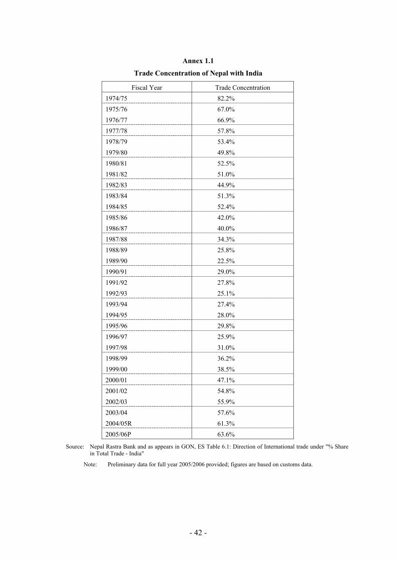
- 42 -

Annex 1.1

Trade Concentration of Nepal with India

Fiscal Year Trade Concentration 1974/75 82.2% 1975/76 67.0% 1976/77 66.9% 1977/78 57.8% 1978/79 53.4% 1979/80 49.8% 1980/81 52.5% 1981/82 51.0% 1982/83 44.9% 1983/84 51.3% 1984/85 52.4% 1985/86 42.0% 1986/87 40.0% 1987/88 34.3% 1988/89 25.8% 1989/90 22.5% 1990/91 29.0% 1991/92 27.8% 1992/93 25.1% 1993/94 27.4% 1994/95 28.0% 1995/96 29.8% 1996/97 25.9% 1997/98 31.0% 1998/99 36.2% 1999/00 38.5% 2000/01 47.1% 2001/02 54.8% 2002/03 55.9% 2003/04 57.6% 2004/05R 61.3% 2005/06P 63.6%

Source: Nepal Rastra Bank and as appears in GON, ES Table 6.1: Direction of International trade under "% Share in Total Trade - India"

Note: Preliminary data for full year 2005/2006 provided; figures are based on customs data.

- 43 -

Annex 2.1

Different Measures of Prices in Nepal In addition to Consumer Price Index, NRB has also begun to publish a number of the price indexes such as WPI, SWRI and core inflation; these are:

The Wholesale Price Index (WPI) has been produced since 2000. This index has added new dimension in looking at the price movement and broadened the horizon and the scope in analyzing price movement in Nepal. The WPI comprises of 71 commodities distinguished between agricultural commodities (49.59 percent), domestic manufactured products (20.37 percent) and imported commodities (30.04 percent). Wholesale Prices are collected from 20 different market centers on fortnightly and monthly basis and 507 observations. (Develop with details in appendix)

The Salary and Wage Rate Index (SWRI, 2004/05 = 100) has been produced since 2001. SRWI includes the salary of employees in the civil service, police, armed police, and army as well as in the public and private corporate sectors. It also includes the wages of labours in agricultural, industrial and construction sectors of eleven different market centers. The trend of the growth rate of salary and wage rate index depicts expenditure pattern in the economy. Increase in per capita income also raises per capita expenditure and savings simultaneously, which ultimately causes an increase in national investment and productivity growth. Altogether 40 observations are made for the salary index and 396 observations for the wage rate index from 11 different market centers each month. Since price stability is the main objective of monetary policy and the money supply is one of the most important determinants of inflation, an appropriate measure of inflation is essential for taking monetary policy decisions. The headline inflation is often volatile and unreliable predictor of the true inflationary trend, core inflation can be a more accurate measure of underlying inflation and can be a useful weapon in the quest for price stability. Monetary policy affects the price after a long lag due to relative price shocks. Sector-specific shocks and economic as well as other policy can temporarily produce noise in the price indices. The core inflation is expected to extract the persistent part of the headline inflation while making monetary policy decision. Temporary shocks can reverse as well. While computing core inflation, food and energy prices are excluded from the CPI basket. Although, exclusion method involves subjectivity in deciding items to be excluded from the basket and suffers from a potential risk of information loss, the core inflation measure uses exclusion principle which is readily understandable, easy to compute, transparent variable. Thus, core inflation has been used to measure the trend on general level of prices. It aims to capture permanent trend by eliminating the effects of temporary disturbance or shocks on average consumer prices or headline inflation. In Nepal, core inflation has been published since mid-October 2005. Rice and rice products, vegetables and fruits, fuel-light-and-water, and transport are excluded from the CPI while computing core inflation. The WPI, SWRI and core CPI indices are provided below for the references:

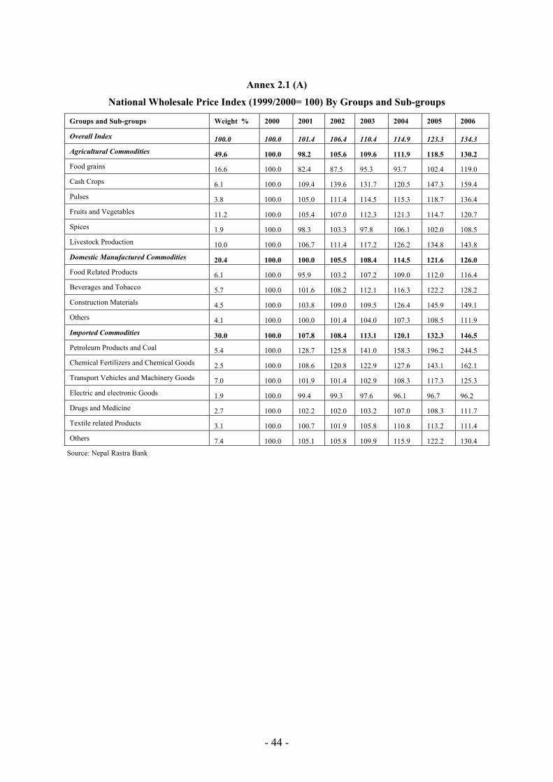
- 44 -

Annex 2.1 (A)

National Wholesale Price Index (1999/2000= 100) By Groups and Sub-groups

Groups and Sub-groups Weight % 2000 2001 2002 2003 2004 2005 2006

Overall Index 100.0 100.0 101.4 106.4 110.4 114.9 123.3 134.3 Agricultural Commodities 49.6 100.0 98.2 105.6 109.6 111.9 118.5 130.2 Food grains 16.6 100.0 82.4 87.5 95.3 93.7 102.4 119.0 Cash Crops 6.1 100.0 109.4 139.6 131.7 120.5 147.3 159.4 Pulses 3.8 100.0 105.0 111.4 114.5 115.3 118.7 136.4 Fruits and Vegetables 11.2 100.0 105.4 107.0 112.3 121.3 114.7 120.7 Spices 1.9 100.0 98.3 103.3 97.8 106.1 102.0 108.5 Livestock Production 10.0 100.0 106.7 111.4 117.2 126.2 134.8 143.8

Domestic Manufactured Commodities 20.4 100.0 100.0 105.5 108.4 114.5 121.6 126.0 Food Related Products 6.1 100.0 95.9 103.2 107.2 109.0 112.0 116.4 Beverages and Tobacco 5.7 100.0 101.6 108.2 112.1 116.3 122.2 128.2 Construction Materials 4.5 100.0 103.8 109.0 109.5 126.4 145.9 149.1 Others 4.1 100.0 100.0 101.4 104.0 107.3 108.5 111.9

Imported Commodities 30.0 100.0 107.8 108.4 113.1 120.1 132.3 146.5 Petroleum Products and Coal 5.4 100.0 128.7 125.8 141.0 158.3 196.2 244.5 Chemical Fertilizers and Chemical Goods 2.5 100.0 108.6 120.8 122.9 127.6 143.1 162.1 Transport Vehicles and Machinery Goods 7.0 100.0 101.9 101.4 102.9 108.3 117.3 125.3 Electric and electronic Goods 1.9 100.0 99.4 99.3 97.6 96.1 96.7 96.2 Drugs and Medicine 2.7 100.0 102.2 102.0 103.2 107.0 108.3 111.7 Textile related Products 3.1 100.0 100.7 101.9 105.8 110.8 113.2 111.4 Others 7.4 100.0 105.1 105.8 109.9 115.9 122.2 130.4

Source: Nepal Rastra Bank

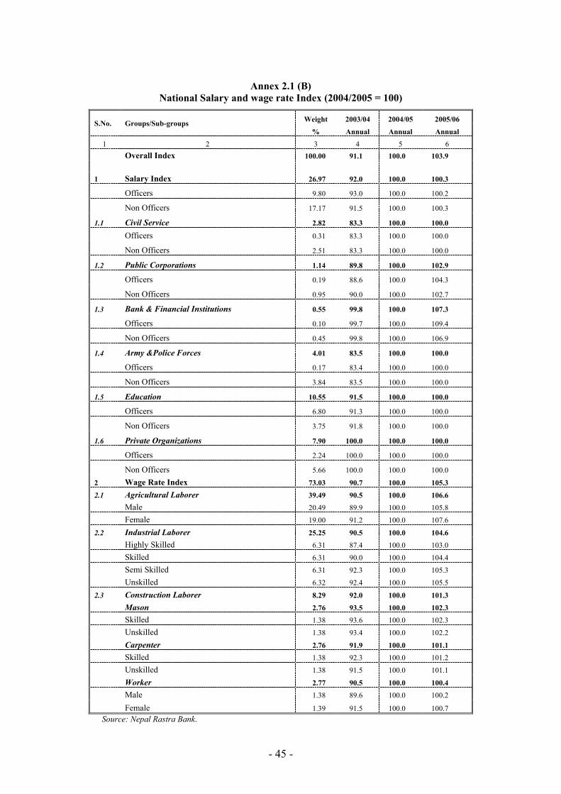
- 45 -

Annex 2.1 (B) National Salary and wage rate Index (2004/2005 = 100)

S.No. Groups/Sub-groups Weight 2003/04 2004/05 2005/06

% Annual Annual Annual 1 2 3 4 5 6

Overall Index 100.00 91.1 100.0 103.9 1 Salary Index 26.97 92.0 100.0 100.3

Officers 9.80 93.0 100.0 100.2

Non Officers 17.17 91.5 100.0 100.3

1.1 Civil Service 2.82 83.3 100.0 100.0

Officers 0.31 83.3 100.0 100.0

Non Officers 2.51 83.3 100.0 100.0

1.2 Public Corporations 1.14 89.8 100.0 102.9

Officers 0.19 88.6 100.0 104.3

Non Officers 0.95 90.0 100.0 102.7

1.3 Bank & Financial Institutions 0.55 99.8 100.0 107.3

Officers 0.10 99.7 100.0 109.4

Non Officers 0.45 99.8 100.0 106.9

1.4 Army &Police Forces 4.01 83.5 100.0 100.0

Officers 0.17 83.4 100.0 100.0

Non Officers 3.84 83.5 100.0 100.0

1.5 Education 10.55 91.5 100.0 100.0

Officers 6.80 91.3 100.0 100.0

Non Officers 3.75 91.8 100.0 100.0

1.6 Private Organizations 7.90 100.0 100.0 100.0

Officers 2.24 100.0 100.0 100.0

Non Officers 5.66 100.0 100.0 100.0

2 Wage Rate Index 73.03 90.7 100.0 105.3

2.1 Agricultural Laborer 39.49 90.5 100.0 106.6 Male 20.49 89.9 100.0 105.8

Female 19.00 91.2 100.0 107.6

2.2 Industrial Laborer 25.25 90.5 100.0 104.6 Highly Skilled 6.31 87.4 100.0 103.0

Skilled 6.31 90.0 100.0 104.4

Semi Skilled 6.31 92.3 100.0 105.3

Unskilled 6.32 92.4 100.0 105.5

2.3 Construction Laborer 8.29 92.0 100.0 101.3 Mason 2.76 93.5 100.0 102.3 Skilled 1.38 93.6 100.0 102.3

Unskilled 1.38 93.4 100.0 102.2

Carpenter 2.76 91.9 100.0 101.1 Skilled 1.38 92.3 100.0 101.2

Unskilled 1.38 91.5 100.0 101.1

Worker 2.77 90.5 100.0 100.4 Male 1.38 89.6 100.0 100.2

Female 1.39 91.5 100.0 100.7 Source: Nepal Rastra Bank.

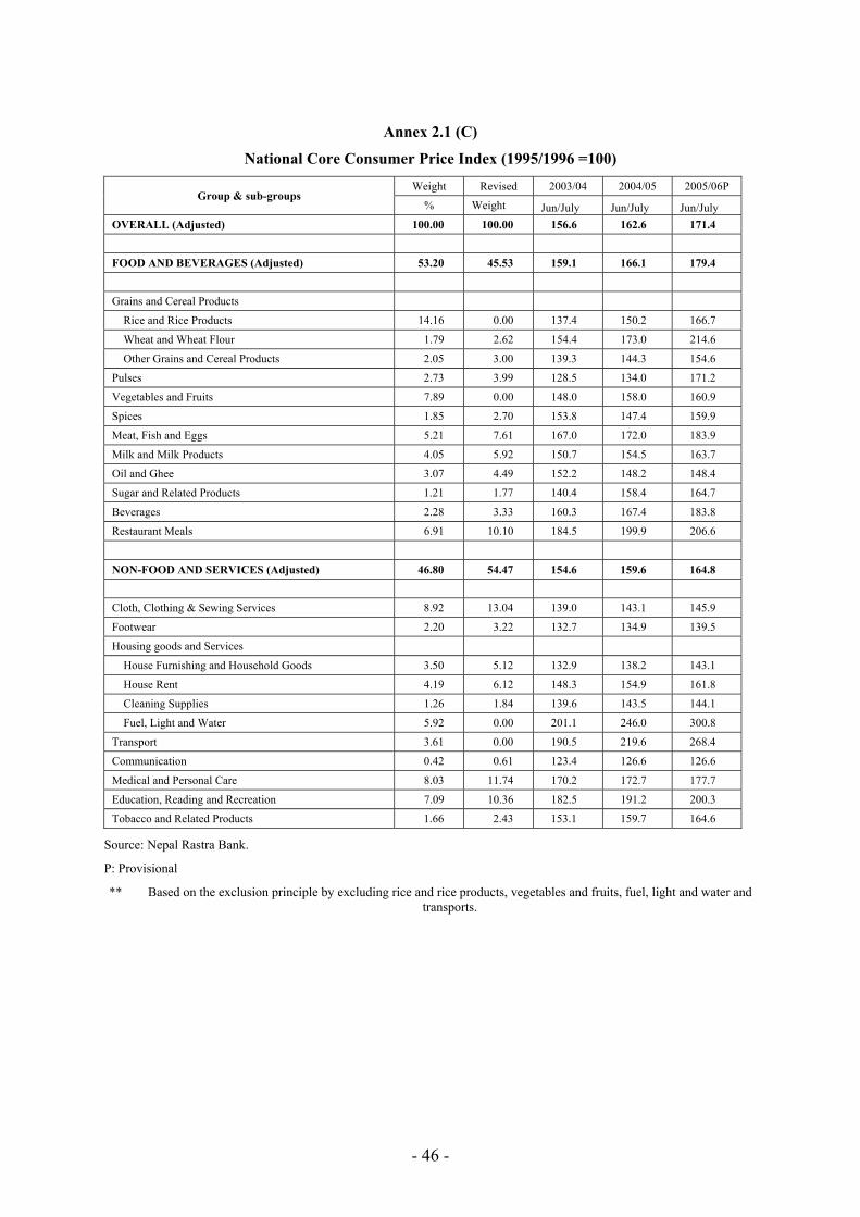
- 46 -

Annex 2.1 (C)

National Core Consumer Price Index (1995/1996 =100)

Group & sub-groups Weight Revised 2003/04 2004/05 2005/06P

% Weight Jun/July Jun/July Jun/July OVERALL (Adjusted) 100.00 100.00 156.6 162.6 171.4

FOOD AND BEVERAGES (Adjusted) 53.20 45.53 159.1 166.1 179.4

Grains and Cereal Products

Rice and Rice Products 14.16 0.00 137.4 150.2 166.7

Wheat and Wheat Flour 1.79 2.62 154.4 173.0 214.6

Other Grains and Cereal Products 2.05 3.00 139.3 144.3 154.6

Pulses 2.73 3.99 128.5 134.0 171.2

Vegetables and Fruits 7.89 0.00 148.0 158.0 160.9

Spices 1.85 2.70 153.8 147.4 159.9

Meat, Fish and Eggs 5.21 7.61 167.0 172.0 183.9

Milk and Milk Products 4.05 5.92 150.7 154.5 163.7

Oil and Ghee 3.07 4.49 152.2 148.2 148.4

Sugar and Related Products 1.21 1.77 140.4 158.4 164.7

Beverages 2.28 3.33 160.3 167.4 183.8

Restaurant Meals 6.91 10.10 184.5 199.9 206.6

NON-FOOD AND SERVICES (Adjusted) 46.80 54.47 154.6 159.6 164.8

Cloth, Clothing & Sewing Services 8.92 13.04 139.0 143.1 145.9

Footwear 2.20 3.22 132.7 134.9 139.5

Housing goods and Services

House Furnishing and Household Goods 3.50 5.12 132.9 138.2 143.1

House Rent 4.19 6.12 148.3 154.9 161.8

Cleaning Supplies 1.26 1.84 139.6 143.5 144.1

Fuel, Light and Water 5.92 0.00 201.1 246.0 300.8

Transport 3.61 0.00 190.5 219.6 268.4

Communication 0.42 0.61 123.4 126.6 126.6

Medical and Personal Care 8.03 11.74 170.2 172.7 177.7

Education, Reading and Recreation 7.09 10.36 182.5 191.2 200.3

Tobacco and Related Products 1.66 2.43 153.1 159.7 164.6

Source: Nepal Rastra Bank.

P: Provisional

** Based on the exclusion principle by excluding rice and rice products, vegetables and fruits, fuel, light and water and transports.

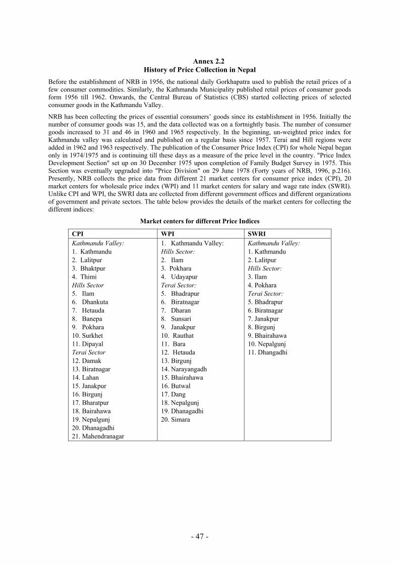
- 47 -

Annex 2.2 History of Price Collection in Nepal

Before the establishment of NRB in 1956, the national daily Gorkhapatra used to publish the retail prices of a few consumer commodities. Similarly, the Kathmandu Municipality published retail prices of consumer goods form 1956 till 1962. Onwards, the Central Bureau of Statistics (CBS) started collecting prices of selected consumer goods in the Kathmandu Valley.

NRB has been collecting the prices of essential consumers’ goods since its establishment in 1956. Initially the number of consumer goods was 15, and the data collected was on a fortnightly basis. The number of consumer goods increased to 31 and 46 in 1960 and 1965 respectively. In the beginning, un-weighted price index for Kathmandu valley was calculated and published on a regular basis since 1957. Terai and Hill regions were added in 1962 and 1963 respectively. The publication of the Consumer Price Index (CPI) for whole Nepal began only in 1974/1975 and is continuing till these days as a measure of the price level in the country. "Price Index Development Section" set up on 30 December 1975 upon completion of Family Budget Survey in 1975. This Section was eventually upgraded into "Price Division" on 29 June 1978 (Forty years of NRB, 1996, p.216). Presently, NRB collects the price data from different 21 market centers for consumer price index (CPI), 20 market centers for wholesale price index (WPI) and 11 market centers for salary and wage rate index (SWRI). Unlike CPI and WPI, the SWRI data are collected from different government offices and different organizations of government and private sectors. The table below provides the details of the market centers for collecting the different indices:

Market centers for different Price Indices

CPI WPI SWRI Kathmandu Valley: 1. Kathmandu 2. Lalitpur 3. Bhaktpur 4. Thimi Hills Sector 5. Ilam 6. Dhankuta 7. Hetauda 8. Banepa 9. Pokhara 10. Surkhet 11. Dipayal Terai Sector 12. Damak 13. Biratnagar 14. Lahan 15. Janakpur 16. Birgunj 17. Bharatpur 18. Bairahawa 19. Nepalgunj 20. Dhanagadhi 21. Mahendranagar

1. Kathmandu Valley: Hills Sector: 2. Ilam 3. Pokhara 4. Udayapur Terai Sector: 5. Bhadrapur 6. Biratnagar 7. Dharan 8. Sunsari 9. Janakpur 10. Rauthat 11. Bara 12. Hetauda 13. Birgunj 14. Narayangadh 15. Bhairahawa 16. Butwal 17. Dang 18. Nepalgunj 19. Dhanagadhi 20. Simara

Kathmandu Valley: 1. Kathmandu 2. Lalitpur Hills Sector: 3. Ilam 4. Pokhara Terai Sector: 5. Bhadrapur 6. Biratnagar 7. Janakpur 8. Birgunj 9. Bhairahawa 10. Nepalgunj 11. Dhangadhi

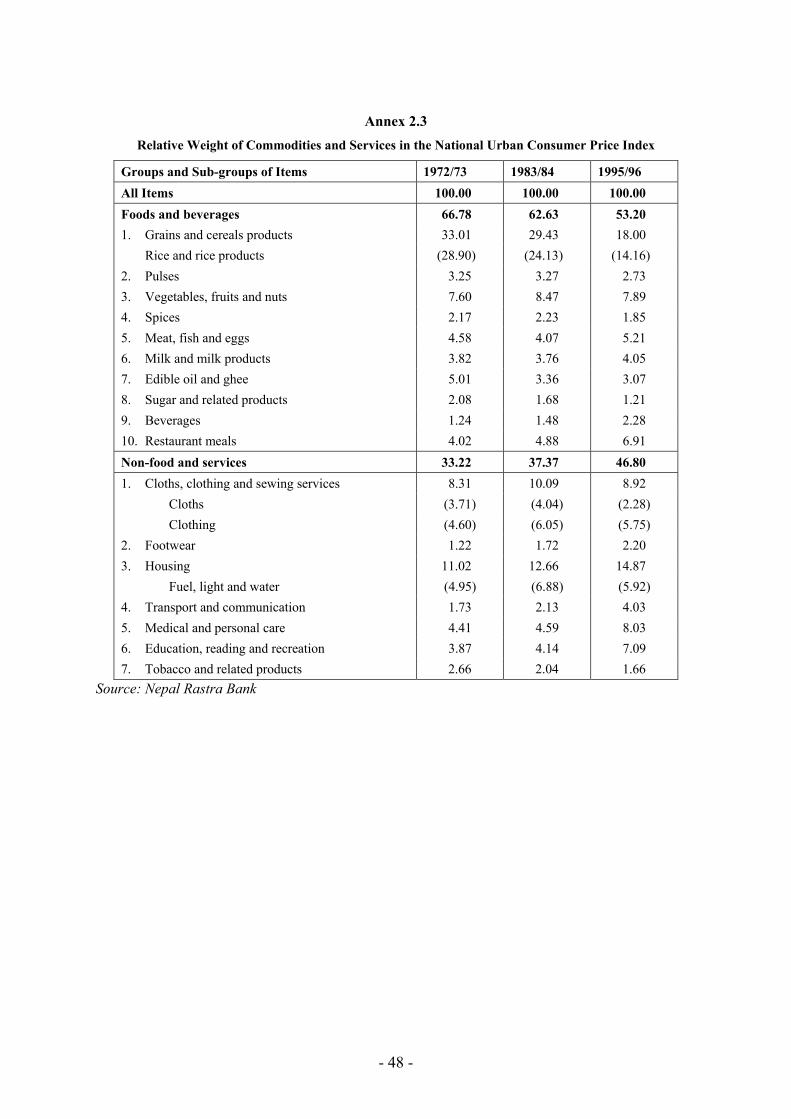
- 48 -

Annex 2.3 Relative Weight of Commodities and Services in the National Urban Consumer Price Index

Groups and Sub-groups of Items 1972/73 1983/84 1995/96 All Items 100.00 100.00 100.00 Foods and beverages 66.78 62.63 53.20 1. Grains and cereals products 33.01 29.43 18.00 Rice and rice products (28.90) (24.13) (14.16) 2. Pulses 3.25 3.27 2.73 3. Vegetables, fruits and nuts 7.60 8.47 7.89 4. Spices 2.17 2.23 1.85 5. Meat, fish and eggs 4.58 4.07 5.21 6. Milk and milk products 3.82 3.76 4.05 7. Edible oil and ghee 5.01 3.36 3.07 8. Sugar and related products 2.08 1.68 1.21 9. Beverages 1.24 1.48 2.28 10. Restaurant meals 4.02 4.88 6.91 Non-food and services 33.22 37.37 46.80 1. Cloths, clothing and sewing services 8.31 10.09 8.92 Cloths (3.71) (4.04) (2.28) Clothing (4.60) (6.05) (5.75) 2. Footwear 1.22 1.72 2.20 3. Housing 11.02 12.66 14.87 Fuel, light and water (4.95) (6.88) (5.92) 4. Transport and communication 1.73 2.13 4.03 5. Medical and personal care 4.41 4.59 8.03 6. Education, reading and recreation 3.87 4.14 7.09 7. Tobacco and related products 2.66 2.04 1.66

Source: Nepal Rastra Bank

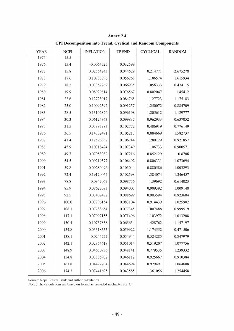
- 49 -

Annex 2.4

CPI Decomposition into Trend, Cyclical and Random Components

YEAR NCPI INFLATION TREND CYCLICAL RANDOM 1975 15.5

1976 15.4 -0.0064725 0.032599

1977 15.8 0.02564243 0.044629 0.214771 2.675278

1978 17.6 0.10788896 0.056268 1.186574 1.615934

1979 18.2 0.03352269 0.066935 1.056333 0.474115

1980 19.9 0.08929814 0.076567 0.802047 1.45412

1981 22.6 0.12723017 0.084765 1.27723 1.175183

1982 25.0 0.10092592 0.091257 1.250072 0.884709

1983 28.5 0.13102826 0.096198 1.205612 1.129777

1984 30.3 0.06124363 0.099837 0.962933 0.637052

1985 31.5 0.03883983 0.102772 0.486919 0.776149

1986 36.5 0.14732471 0.105217 0.884669 1.582737

1987 41.4 0.12596862 0.106744 1.280129 0.921857

1988 45.9 0.10318424 0.107349 1.06733 0.900571

1989 49.7 0.07953982 0.107216 0.852129 0.8706

1990 54.5 0.09219577 0.106492 0.806331 1.073694

1991 59.8 0.09280496 0.105044 0.880586 1.003293

1992 72.4 0.19120064 0.102598 1.384074 1.346457

1993 78.8 0.0847067 0.098756 1.39692 0.614023

1994 85.9 0.08627083 0.094007 0.909392 1.009148

1995 92.5 0.07402482 0.088699 0.903594 0.923604

1996 100.0 0.07796154 0.083104 0.914439 1.025902

1997 108.1 0.07788654 0.077345 1.007488 0.999519

1998 117.1 0.07997155 0.071496 1.103972 1.013208

1999 130.4 0.10757838 0.065634 1.428762 1.147197

2000 134.8 0.03318555 0.059922 1.174552 0.471506

2001 138.1 0.0244272 0.054944 0.524285 0.847979

2002 142.1 0.02854618 0.051014 0.519207 1.077756

2003 148.9 0.04650936 0.048141 0.779535 1.239332

2004 154.8 0.03885902 0.046112 0.925667 0.910384

2005 161.8 0.04422704 0.044694 0.929491 1.064608

2006 174.3 0.07441695 0.043585 1.361056 1.254458

Source: Nepal Rastra Bank and author calculation. Note ; The calculations are based on formulae provided in chapter 2(2.3).

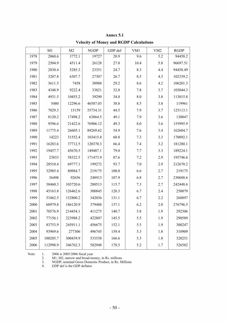
- 50 -

Annex 5.1

Velocity of Money and RGDP Calculations

M1 M2 NGDP GDP def VM1 VM2 RGDP 1978 2060.6 3772.1 19727 20.9 9.6 5.2 94458.2

1979 2504.9 4511.4 26128 27.0 10.4 5.8 96697.51

1980 2830.4 5285.3 23351 24.7 8.3 4.4 94458.49

1981 3207.8 6307.7 27307 26.7 8.5 4.3 102339.2

1982 3611.5 7458 30988 29.2 8.6 4.2 106201.3

1983 4348.9 9222.4 33821 32.8 7.8 3.7 103044.3

1984 4931.5 10455.2 39290 34.8 8.0 3.8 113015.8

1985 5480 12296.6 46587.03 38.8 8.5 3.8 119961

1986 7029.3 15159 55734.31 44.5 7.9 3.7 125113.1

1987 8120.2 17498.2 63864.5 49.1 7.9 3.6 130047

1988 9596.6 21422.6 76906.12 49.3 8.0 3.6 155995.9

1989 11775.4 26605.1 89269.62 54.9 7.6 3.4 162604.7

1990 14223 31552.4 103415.8 60.8 7.3 3.3 170092.1

1991 16283.6 37712.5 120370.3 66.4 7.4 3.2 181280.1

1992 19457.7 45670.5 149487.1 79.0 7.7 3.3 189224.1

1993 23833 58322.5 171473.9 87.6 7.2 2.9 195746.6

1994 28510.4 69777.1 199272 93.7 7.0 2.9 212670.2

1995 32985.4 80984.7 219175 100.0 6.6 2.7 219175

1996 36498 92656 248913 107.9 6.8 2.7 230688.6

1997 38460.3 103720.6 280513 115.7 7.3 2.7 242448.6

1998 45163.8 126462.6 300845 120.3 6.7 2.4 250079

1999 51062.5 152800.2 342036 131.1 6.7 2.2 260897

2000 60979.8 186120.9 379488 137.1 6.2 2.0 276796.5

2001 70576.9 214454.1 411275 140.7 5.8 1.9 292306

2002 77156.1 223988.2 422807 145.5 5.5 1.9 290589

2003 83753.9 245911.1 456675 152.1 5.5 1.9 300247

2004 93969.6 277306 496745 159.4 5.3 1.8 310909

2005 100205.7 300439.9 533538 166.6 5.3 1.8 320251

2006 112998.9 346762.3 582948 178.5 5.2 1.7 326582

Note: 1. 2006 is 2005/2006 fiscal year 2. M1, M2, narrow and broad money, in Rs. millions 3. NGDP, nominal Gross Domestic Product, in Rs. Millions 4. GDP def is the GDP deflator

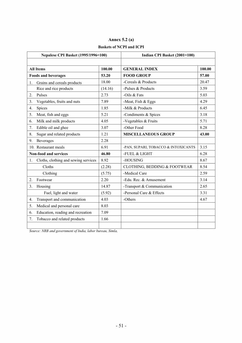
- 51 -

Annex 5.2 (a) Baskets of NCPI and ICPI

Nepalese CPI Basket (1995/1996=100) Indian CPI Basket (2001=100)

All Items 100.00 GENERAL INDEX 100.00 Foods and beverages 53.20 FOOD GROUP 57.00

1. Grains and cereals products 18.00 -Cereals & Products 20.47 Rice and rice products (14.16) -Pulses & Products 3.59 2. Pulses 2.73 -Oils & Fats 5.03 3. Vegetables, fruits and nuts 7.89 -Meat, Fish & Eggs 4.29 4. Spices 1.85 -Milk & Products 6.45 5. Meat, fish and eggs 5.21 -Condiments & Spices 3.18 6. Milk and milk products 4.05 -Vegetables & Fruits 5.71 7. Edible oil and ghee 3.07 -Other Food 8.28 8. Sugar and related products 1.21 MISCELLANEOUS GROUP 43.00 9. Beverages 2.28 10. Restaurant meals 6.91 -PAN, SUPARI, TOBACCO & INTOXICANTS 3.15 Non-food and services 46.80 -FUEL & LIGHT 6.28 1. Cloths, clothing and sewing services 8.92 -HOUSING 8.67 Cloths (2.28) CLOTHING, BEDDING & FOOTWEAR 8.54 Clothing (5.75) -Medical Care 2.59 2. Footwear 2.20 -Edu. Rec. & Amusement 3.14 3. Housing 14.87 -Transport & Communication 2.65 Fuel, light and water (5.92) -Personal Care & Effects 3.31 4. Transport and communication 4.03 -Others 4.67 5. Medical and personal care 8.03 6. Education, reading and recreation 7.09 7. Tobacco and related products 1.66 Source: NRB and government of India, labor bureau, Simla,

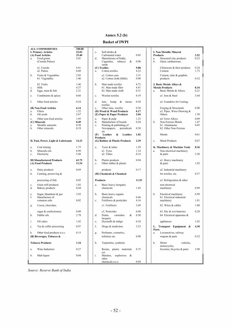
- 52 -

Annex 5.2 (b)

Basket of IWPI

ALL COMMODITIES 100.00 I. Primary Articles 22.03 c. Soft drinks & I. Non-Metallic Mineral (A) Food Articles 15.40 Carbonated water 0.05 Products 2.52 a. Food grains 5.01 d. Manufacture of biddy, a. Structural clay products 0.23 (Cereals Pulses)

Cigarettes, tobacco &

zarda 0.98

b. Glass, earthenware,

a1. Cereals 4.41 (C) Textiles 9.80 Chinaware & their products 0.24 a2. Pulses 0.60 a. Cotton textiles 4.22 Cement 1.73 b. Fruits & Vegetables 2.92 a1. Cotton yarn 3.31 Cement, slate & graphite b1. Vegetables 1.46

a2. Cotton cloth (Mills) 0.90

products 0.32

b2. Fruits 1.46 b. Man made textiles 4.72 J. Basic Metals Alloys & c. Milk 4.37 b1. Man made fiber 4.41 Metals Products 8.34 d. Eggs, meat & fish 2.21

b2. Man made cloth 0.31

a. Basic Metals & Alloys 6.21

e. Condiments & spices 0.66

c. Woolen textiles 0.19

a1. Iron & Steel 3.64

f. Other food articles 0.24

d. Jute, hemp & mesta textiles

0.38

a2. Foundries for Casting,

(B) Non-Food Articles 6.14 e. Other misc. textiles 0.30 Forging & Structurals 0.90 a. Fibers 1.52 (D) Wood & Wood Products 0.17 a3. Pipes, Wires Drawing & b. Oil seeds 2.67 (E) Paper & Paper Products 2.04 Others 1.59 c. Other non-food articles 1.95 a. Paper & pulp 1.23 a4. Ferro Alloys 0.09 (C) Minerals 0.49 b. Manufacture of boards 0.24 b. Non-Ferrous Metals 1.47 a. Metallic minerals 0.30 c. Printing & publishing of b1. Aluminums 0.85 b. Other minerals 0.19

Newspapers, periodicals

etc 0.58

b2. Other Non-Ferrous

(F) Leather & Leather Products

1.02

Metals 0.61

II. Fuel, Power, Light & Lubricants 14.23

(G) Rubber & Plastic Products 2.39

c. Metal Products 0.67

a. Coal mining 1.75 a. Tyres & tubes 1.29 K. Machinery & Machine Tools 8.36 b. Minerals oils 6.99 a1. Tyres 1.14 a. Non-electrical machinery c. Electricity 5.48

a2. Tubes 0.14

& parts 3.38

III.Manufactured Products 63.75 b. Plastic products 0.94 a1. Heavy machinery (A) Food Products 11.54

c. Other rubber & plastic

& parts 1.82

a. Dairy products 0.69 products 0.17 a2. Industrial machinery b. Canning, preserving &

(H) Chemicals & Chemical

for textiles, etc. 0.57

processing of fish 0.05 Products 11.93 a3. Refrigeration & other

c. Grain mill products 1.03 a. Basic heavy inorganic non-electrical d. Bakery products 0.44

chemicals 1.45

machinery 0.99

e. Sugar, khandsari & gur 3.93 b. Basic heavy organic b. Electrical machinery 4.99 f. Manufacture of chemicals 0.46 b1. Electrical industrial common salts 0.02

c. Fertilisers & pesticides 4.16

machinery 1.81

g. Cocoa, chocolate,

c1. Fertilisers 3.69

b2. Wires & cables 1.08

sugar & confectionery 0.09 c2. Pesticides 0.48 b3. Dry & wet batteries 0.28 h. Edible oils 2.78

d. Paints, varnishes &

lacquers 0.50

b4. Electrical apparatus &

i. Oil cakes 1.42

e. Dyestuffs & indigo 0.18

appliances 1.82

j. Tea & coffee processing 0.97

f. Drugs & medicines 2.53

L. Transport Equipment & Parts

4.30

k. Other food products n.e.c. 0.15 g. Perfumes, cosmetics, a. Locomotives, railway (B) Beverages, Tobacco &

toiletries etc. 0.98

wagons & parts 0.32

Tobacco Products 1.34

h. Turpentine, synthetic

b. Motor vehicles, motorcycles,

a. Wine Industries 0.27

Resins, plastic materials ect.

0.75

Scooters, bicycles & parts 3.98

b. Malt liquor 0.04

i. Matches, explosives & other

chemicals n.e.c. 0.94

Source: Reserve Bank of India

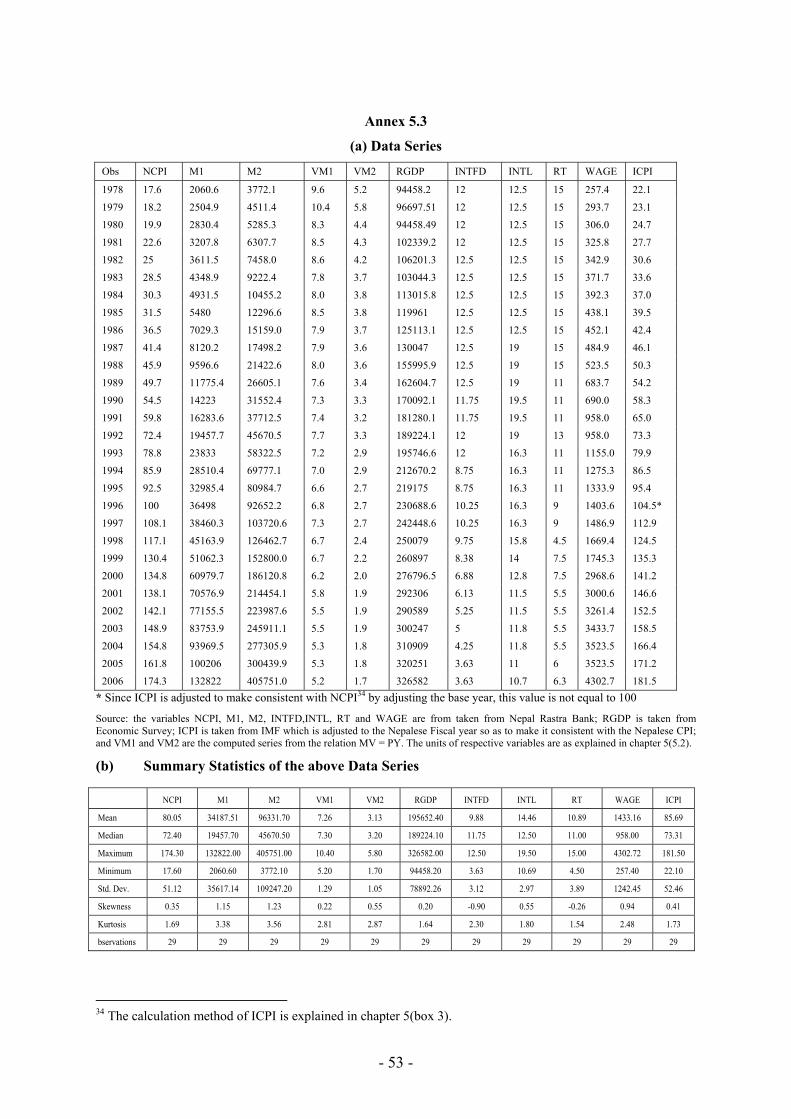
- 53 -

Annex 5.3

(a) Data Series

Obs NCPI M1 M2 VM1 VM2 RGDP INTFD INTL RT WAGE ICPI

1978 17.6 2060.6 3772.1 9.6 5.2 94458.2 12 12.5 15 257.4 22.1

1979 18.2 2504.9 4511.4 10.4 5.8 96697.51 12 12.5 15 293.7 23.1

1980 19.9 2830.4 5285.3 8.3 4.4 94458.49 12 12.5 15 306.0 24.7

1981 22.6 3207.8 6307.7 8.5 4.3 102339.2 12 12.5 15 325.8 27.7

1982 25 3611.5 7458.0 8.6 4.2 106201.3 12.5 12.5 15 342.9 30.6

1983 28.5 4348.9 9222.4 7.8 3.7 103044.3 12.5 12.5 15 371.7 33.6

1984 30.3 4931.5 10455.2 8.0 3.8 113015.8 12.5 12.5 15 392.3 37.0

1985 31.5 5480 12296.6 8.5 3.8 119961 12.5 12.5 15 438.1 39.5

1986 36.5 7029.3 15159.0 7.9 3.7 125113.1 12.5 12.5 15 452.1 42.4

1987 41.4 8120.2 17498.2 7.9 3.6 130047 12.5 19 15 484.9 46.1

1988 45.9 9596.6 21422.6 8.0 3.6 155995.9 12.5 19 15 523.5 50.3

1989 49.7 11775.4 26605.1 7.6 3.4 162604.7 12.5 19 11 683.7 54.2

1990 54.5 14223 31552.4 7.3 3.3 170092.1 11.75 19.5 11 690.0 58.3

1991 59.8 16283.6 37712.5 7.4 3.2 181280.1 11.75 19.5 11 958.0 65.0

1992 72.4 19457.7 45670.5 7.7 3.3 189224.1 12 19 13 958.0 73.3

1993 78.8 23833 58322.5 7.2 2.9 195746.6 12 16.3 11 1155.0 79.9

1994 85.9 28510.4 69777.1 7.0 2.9 212670.2 8.75 16.3 11 1275.3 86.5

1995 92.5 32985.4 80984.7 6.6 2.7 219175 8.75 16.3 11 1333.9 95.4

1996 100 36498 92652.2 6.8 2.7 230688.6 10.25 16.3 9 1403.6 104.5*

1997 108.1 38460.3 103720.6 7.3 2.7 242448.6 10.25 16.3 9 1486.9 112.9

1998 117.1 45163.9 126462.7 6.7 2.4 250079 9.75 15.8 4.5 1669.4 124.5

1999 130.4 51062.3 152800.0 6.7 2.2 260897 8.38 14 7.5 1745.3 135.3

2000 134.8 60979.7 186120.8 6.2 2.0 276796.5 6.88 12.8 7.5 2968.6 141.2

2001 138.1 70576.9 214454.1 5.8 1.9 292306 6.13 11.5 5.5 3000.6 146.6

2002 142.1 77155.5 223987.6 5.5 1.9 290589 5.25 11.5 5.5 3261.4 152.5

2003 148.9 83753.9 245911.1 5.5 1.9 300247 5 11.8 5.5 3433.7 158.5

2004 154.8 93969.5 277305.9 5.3 1.8 310909 4.25 11.8 5.5 3523.5 166.4

2005 161.8 100206 300439.9 5.3 1.8 320251 3.63 11 6 3523.5 171.2

2006 174.3 132822 405751.0 5.2 1.7 326582 3.63 10.7 6.3 4302.7 181.5 * Since ICPI is adjusted to make consistent with NCPI34 by adjusting the base year, this value is not equal to 100

Source: the variables NCPI, M1, M2, INTFD,INTL, RT and WAGE are from taken from Nepal Rastra Bank; RGDP is taken from Economic Survey; ICPI is taken from IMF which is adjusted to the Nepalese Fiscal year so as to make it consistent with the Nepalese CPI; and VM1 and VM2 are the computed series from the relation MV = PY. The units of respective variables are as explained in chapter 5(5.2).

(b) Summary Statistics of the above Data Series NCPI M1 M2 VM1 VM2 RGDP INTFD INTL RT WAGE ICPI

Mean 80.05 34187.51 96331.70 7.26 3.13 195652.40 9.88 14.46 10.89 1433.16 85.69

Median 72.40 19457.70 45670.50 7.30 3.20 189224.10 11.75 12.50 11.00 958.00 73.31

Maximum 174.30 132822.00 405751.00 10.40 5.80 326582.00 12.50 19.50 15.00 4302.72 181.50

Minimum 17.60 2060.60 3772.10 5.20 1.70 94458.20 3.63 10.69 4.50 257.40 22.10

Std. Dev. 51.12 35617.14 109247.20 1.29 1.05 78892.26 3.12 2.97 3.89 1242.45 52.46

Skewness 0.35 1.15 1.23 0.22 0.55 0.20 -0.90 0.55 -0.26 0.94 0.41

Kurtosis 1.69 3.38 3.56 2.81 2.87 1.64 2.30 1.80 1.54 2.48 1.73

bservations 29 29 29 29 29 29 29 29 29 29 29

34 The calculation method of ICPI is explained in chapter 5(box 3).

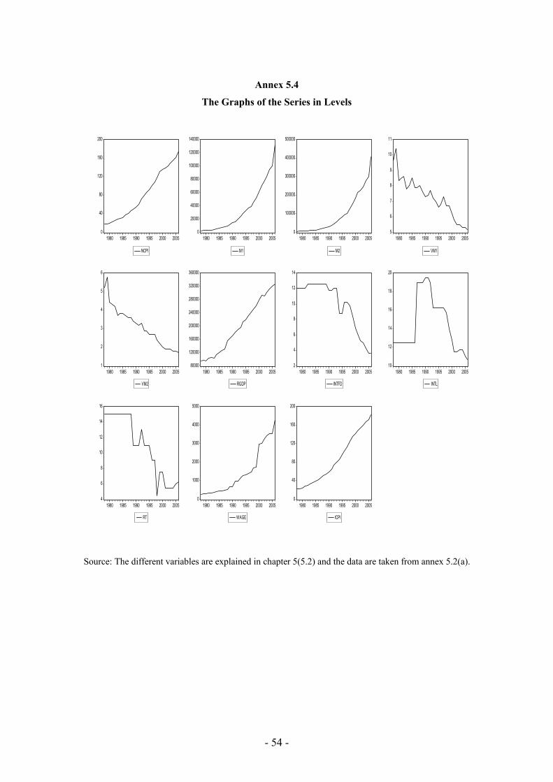
- 54 -

Annex 5.4

The Graphs of the Series in Levels

0

40

80

120

160

200

1980 1985 1990 1995 2000 2005

NCPI

0

20000

40000

60000

80000

100000

120000

140000

1980 1985 1990 1995 2000 2005

M1

0

100000

200000

300000

400000

500000

1980 1985 1990 1995 2000 2005

M2

5

6

7

8

9

10

11

1980 1985 1990 1995 2000 2005

VM1

1

2

3

4

5

6

1980 1985 1990 1995 2000 2005

VM2

80000

120000

160000

200000

240000

280000

320000

360000

1980 1985 1990 1995 2000 2005

RGDP

2

4

6

8

10

12

14

1980 1985 1990 1995 2000 2005

INTFD

10

12

14

16

18

20

1980 1985 1990 1995 2000 2005

INTL

4

6

8

10

12

14

16

1980 1985 1990 1995 2000 2005

RT

0

1000

2000

3000

4000

5000

1980 1985 1990 1995 2000 2005

WAGE

0

40

80

120

160

200

1980 1985 1990 1995 2000 2005

ICPI

Source: The different variables are explained in chapter 5(5.2) and the data are taken from annex 5.2(a).

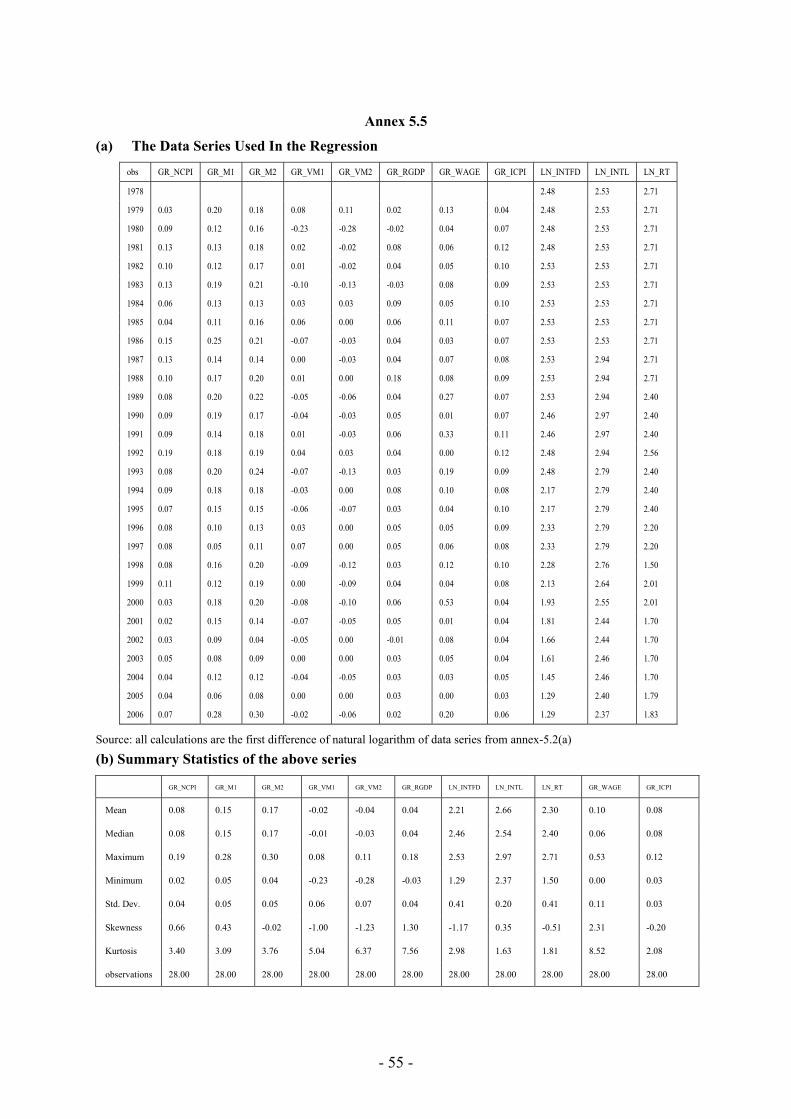
- 55 -

Annex 5.5

(a) The Data Series Used In the Regression

obs GR_NCPI GR_M1 GR_M2 GR_VM1 GR_VM2 GR_RGDP GR_WAGE GR_ICPI LN_INTFD LN_INTL LN_RT

1978 2.48 2.53 2.71

1979 0.03 0.20 0.18 0.08 0.11 0.02 0.13 0.04 2.48 2.53 2.71

1980 0.09 0.12 0.16 -0.23 -0.28 -0.02 0.04 0.07 2.48 2.53 2.71

1981 0.13 0.13 0.18 0.02 -0.02 0.08 0.06 0.12 2.48 2.53 2.71

1982 0.10 0.12 0.17 0.01 -0.02 0.04 0.05 0.10 2.53 2.53 2.71

1983 0.13 0.19 0.21 -0.10 -0.13 -0.03 0.08 0.09 2.53 2.53 2.71

1984 0.06 0.13 0.13 0.03 0.03 0.09 0.05 0.10 2.53 2.53 2.71

1985 0.04 0.11 0.16 0.06 0.00 0.06 0.11 0.07 2.53 2.53 2.71

1986 0.15 0.25 0.21 -0.07 -0.03 0.04 0.03 0.07 2.53 2.53 2.71

1987 0.13 0.14 0.14 0.00 -0.03 0.04 0.07 0.08 2.53 2.94 2.71

1988 0.10 0.17 0.20 0.01 0.00 0.18 0.08 0.09 2.53 2.94 2.71

1989 0.08 0.20 0.22 -0.05 -0.06 0.04 0.27 0.07 2.53 2.94 2.40

1990 0.09 0.19 0.17 -0.04 -0.03 0.05 0.01 0.07 2.46 2.97 2.40

1991 0.09 0.14 0.18 0.01 -0.03 0.06 0.33 0.11 2.46 2.97 2.40

1992 0.19 0.18 0.19 0.04 0.03 0.04 0.00 0.12 2.48 2.94 2.56

1993 0.08 0.20 0.24 -0.07 -0.13 0.03 0.19 0.09 2.48 2.79 2.40

1994 0.09 0.18 0.18 -0.03 0.00 0.08 0.10 0.08 2.17 2.79 2.40

1995 0.07 0.15 0.15 -0.06 -0.07 0.03 0.04 0.10 2.17 2.79 2.40

1996 0.08 0.10 0.13 0.03 0.00 0.05 0.05 0.09 2.33 2.79 2.20

1997 0.08 0.05 0.11 0.07 0.00 0.05 0.06 0.08 2.33 2.79 2.20

1998 0.08 0.16 0.20 -0.09 -0.12 0.03 0.12 0.10 2.28 2.76 1.50

1999 0.11 0.12 0.19 0.00 -0.09 0.04 0.04 0.08 2.13 2.64 2.01

2000 0.03 0.18 0.20 -0.08 -0.10 0.06 0.53 0.04 1.93 2.55 2.01

2001 0.02 0.15 0.14 -0.07 -0.05 0.05 0.01 0.04 1.81 2.44 1.70

2002 0.03 0.09 0.04 -0.05 0.00 -0.01 0.08 0.04 1.66 2.44 1.70

2003 0.05 0.08 0.09 0.00 0.00 0.03 0.05 0.04 1.61 2.46 1.70

2004 0.04 0.12 0.12 -0.04 -0.05 0.03 0.03 0.05 1.45 2.46 1.70

2005 0.04 0.06 0.08 0.00 0.00 0.03 0.00 0.03 1.29 2.40 1.79

2006 0.07 0.28 0.30 -0.02 -0.06 0.02 0.20 0.06 1.29 2.37 1.83

Source: all calculations are the first difference of natural logarithm of data series from annex-5.2(a)

(b) Summary Statistics of the above series

GR_NCPI GR_M1 GR_M2 GR_VM1 GR_VM2 GR_RGDP LN_INTFD LN_INTL LN_RT GR_WAGE GR_ICPI

Mean 0.08 0.15 0.17 -0.02 -0.04 0.04 2.21 2.66 2.30 0.10 0.08

Median 0.08 0.15 0.17 -0.01 -0.03 0.04 2.46 2.54 2.40 0.06 0.08

Maximum 0.19 0.28 0.30 0.08 0.11 0.18 2.53 2.97 2.71 0.53 0.12

Minimum 0.02 0.05 0.04 -0.23 -0.28 -0.03 1.29 2.37 1.50 0.00 0.03

Std. Dev. 0.04 0.05 0.05 0.06 0.07 0.04 0.41 0.20 0.41 0.11 0.03

Skewness 0.66 0.43 -0.02 -1.00 -1.23 1.30 -1.17 0.35 -0.51 2.31 -0.20

Kurtosis 3.40 3.09 3.76 5.04 6.37 7.56 2.98 1.63 1.81 8.52 2.08

observations 28.00 28.00 28.00 28.00 28.00 28.00 28.00 28.00 28.00 28.00 28.00

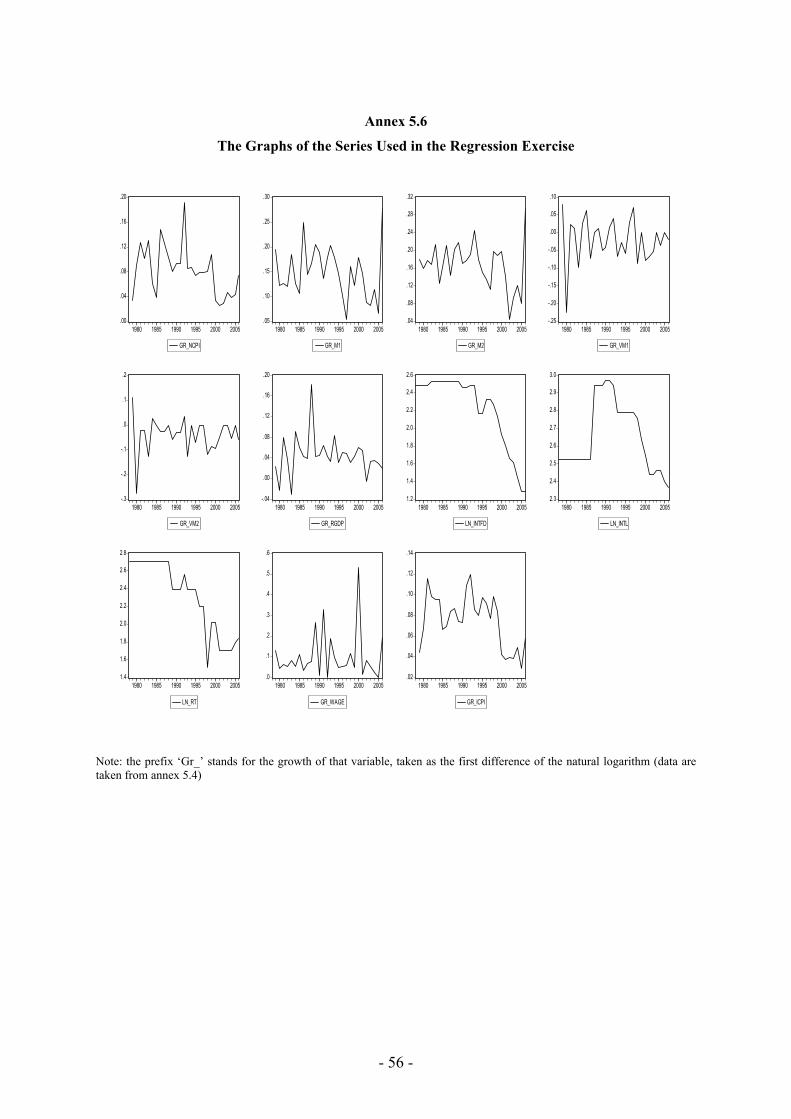
- 56 -

Annex 5.6

The Graphs of the Series Used in the Regression Exercise

.00

.04

.08

.12

.16

.20

1980 1985 1990 1995 2000 2005

GR_NCPI

.05

.10

.15

.20

.25

.30

1980 1985 1990 1995 2000 2005

GR_M1

.04

.08

.12

.16

.20

.24

.28

.32

1980 1985 1990 1995 2000 2005

GR_M2

-.25

-.20

-.15

-.10

-.05

.00

.05

.10

1980 1985 1990 1995 2000 2005

GR_VM1

-.3

-.2

-.1

.0

.1

.2

1980 1985 1990 1995 2000 2005

GR_VM2

-.04

.00

.04

.08

.12

.16

.20

1980 1985 1990 1995 2000 2005

GR_RGDP

1.2

1.4

1.6

1.8

2.0

2.2

2.4

2.6

1980 1985 1990 1995 2000 2005

LN_INTFD

2.3

2.4

2.5

2.6

2.7

2.8

2.9

3.0

1980 1985 1990 1995 2000 2005

LN_INTL

1.4

1.6

1.8

2.0

2.2

2.4

2.6

2.8

1980 1985 1990 1995 2000 2005

LN_RT

.0

.1

.2

.3

.4

.5

.6

1980 1985 1990 1995 2000 2005

GR_WAGE

.02

.04

.06

.08

.10

.12

.14

1980 1985 1990 1995 2000 2005

GR_ICPI

Note: the prefix ‘Gr_’ stands for the growth of that variable, taken as the first difference of the natural logarithm (data are taken from annex 5.4)

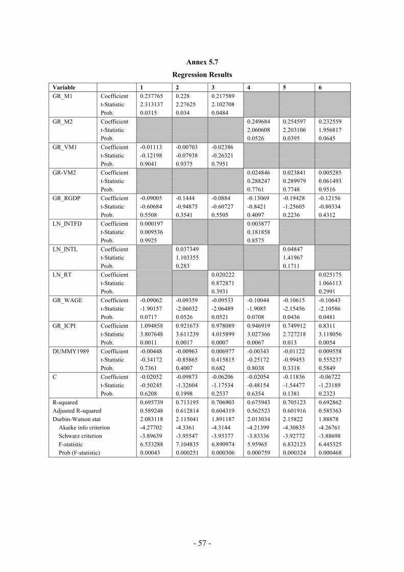
- 57 -

Annex 5.7

Regression Results

Variable 1 2 3 4 5 6 GR_M1 Coefficient 0.237765 0.228 0.217589 t-Statistic 2.313137 2.27625 2.102708 Prob. 0.0315 0.034 0.0484 GR_M2 Coefficient 0.249684 0.254597 0.232559 t-Statistic 2.060608 2.203106 1.956817 Prob. 0.0526 0.0395 0.0645 GR_VM1 Coefficient -0.01113 -0.00703 -0.02386 t-Statistic -0.12198 -0.07938 -0.26321 Prob. 0.9041 0.9375 0.7951 GR-VM2 Coefficient 0.024846 0.023841 0.005285 t-Statistic 0.288247 0.289979 0.061493 Prob. 0.7761 0.7748 0.9516 GR_RGDP Coefficient -0.09005 -0.1444 -0.0884 -0.13069 -0.19428 -0.12156 t-Statistic -0.60684 -0.94875 -0.60727 -0.8421 -1.25605 -0.80334 Prob. 0.5508 0.3541 0.5505 0.4097 0.2236 0.4312 LN_INTFD Coefficient 0.000197 0.003877 t-Statistic 0.009536 0.181858 Prob. 0.9925 0.8575 LN_INTL Coefficient 0.037349 0.04847 t-Statistic 1.103355 1.41967 Prob. 0.283 0.1711 LN_RT Coefficient 0.020222 0.025175 t-Statistic 0.872871 1.066113 Prob. 0.3931 0.2991 GR_WAGE Coefficient -0.09062 -0.09359 -0.09533 -0.10044 -0.10615 -0.10643 t-Statistic -1.90157 -2.06032 -2.06489 -1.9085 -2.15456 -2.10586 Prob. 0.0717 0.0526 0.0521 0.0708 0.0436 0.0481 GR_ICPI Coefficient 1.094858 0.921673 0.978089 0.946919 0.749912 0.8311 t-Statistic 3.807648 3.611239 4.015899 3.027366 2.727218 3.118056 Prob. 0.0011 0.0017 0.0007 0.0067 0.013 0.0054 DUMMY1989 Coefficient -0.00448 -0.00963 0.006977 -0.00343 -0.01122 0.009558 t-Statistic -0.34172 -0.85865 0.415815 -0.25172 -0.99453 0.555237 Prob. 0.7361 0.4007 0.682 0.8038 0.3318 0.5849 C Coefficient -0.02052 -0.09873 -0.06206 -0.02054 -0.11836 -0.06722 t-Statistic -0.50245 -1.32604 -1.17534 -0.48154 -1.54477 -1.23189 Prob. 0.6208 0.1998 0.2537 0.6354 0.1381 0.2323 R-squared 0.695739 0.713195 0.706903 0.675943 0.705123 0.692862 Adjusted R-squared 0.589248 0.612814 0.604319 0.562523 0.601916 0.585363 Durbin-Watson stat 2.083118 2.115041 1.891187 2.013034 2.15822 1.88878 Akaike info criterion -4.27702 -4.3361 -4.3144 -4.21399 -4.30835 -4.26761 Schwarz criterion -3.89639 -3.95547 -3.93377 -3.83336 -3.92772 -3.88698 F-statistic 6.533288 7.104835 6.890974 5.95965 6.832123 6.445325 Prob (F-statistic) 0.00043 0.000251 0.000306 0.000759 0.000324 0.000468

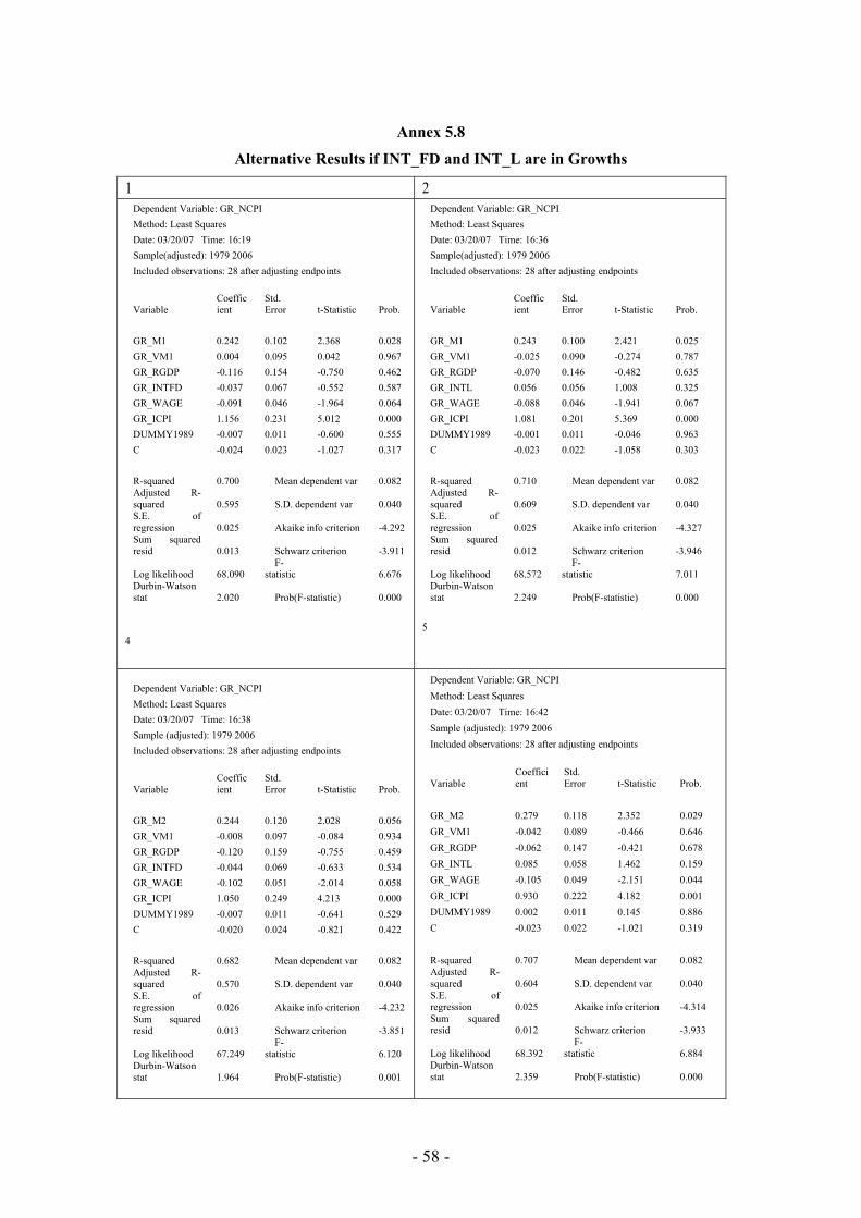
- 58 -

Annex 5.8

Alternative Results if INT_FD and INT_L are in Growths

1 2 Dependent Variable: GR_NCPI Method: Least Squares Date: 03/20/07 Time: 16:19 Sample(adjusted): 1979 2006 Included observations: 28 after adjusting endpoints

Variable Coefficient

Std. Error t-Statistic Prob.

GR_M1 0.242 0.102 2.368 0.028 GR_VM1 0.004 0.095 0.042 0.967 GR_RGDP -0.116 0.154 -0.750 0.462 GR_INTFD -0.037 0.067 -0.552 0.587 GR_WAGE -0.091 0.046 -1.964 0.064 GR_ICPI 1.156 0.231 5.012 0.000 DUMMY1989 -0.007 0.011 -0.600 0.555 C -0.024 0.023 -1.027 0.317 R-squared 0.700 Mean dependent var 0.082 Adjusted R-squared 0.595 S.D. dependent var 0.040 S.E. of regression 0.025 Akaike info criterion -4.292 Sum squared resid 0.013 Schwarz criterion -3.911

Log likelihood 68.090 F-statistic 6.676

Durbin-Watson stat 2.020 Prob(F-statistic) 0.000

4

Dependent Variable: GR_NCPI Method: Least Squares Date: 03/20/07 Time: 16:36 Sample(adjusted): 1979 2006 Included observations: 28 after adjusting endpoints

Variable Coefficient

Std. Error t-Statistic Prob.

GR_M1 0.243 0.100 2.421 0.025 GR_VM1 -0.025 0.090 -0.274 0.787 GR_RGDP -0.070 0.146 -0.482 0.635 GR_INTL 0.056 0.056 1.008 0.325 GR_WAGE -0.088 0.046 -1.941 0.067 GR_ICPI 1.081 0.201 5.369 0.000 DUMMY1989 -0.001 0.011 -0.046 0.963 C -0.023 0.022 -1.058 0.303 R-squared 0.710 Mean dependent var 0.082 Adjusted R-squared 0.609 S.D. dependent var 0.040 S.E. of regression 0.025 Akaike info criterion -4.327 Sum squared resid 0.012 Schwarz criterion -3.946

Log likelihood 68.572 F-statistic 7.011

Durbin-Watson stat 2.249 Prob(F-statistic) 0.000

5

Dependent Variable: GR_NCPI Method: Least Squares Date: 03/20/07 Time: 16:38 Sample (adjusted): 1979 2006 Included observations: 28 after adjusting endpoints

Variable Coefficient

Std. Error t-Statistic Prob.

GR_M2 0.244 0.120 2.028 0.056 GR_VM1 -0.008 0.097 -0.084 0.934 GR_RGDP -0.120 0.159 -0.755 0.459 GR_INTFD -0.044 0.069 -0.633 0.534 GR_WAGE -0.102 0.051 -2.014 0.058 GR_ICPI 1.050 0.249 4.213 0.000 DUMMY1989 -0.007 0.011 -0.641 0.529 C -0.020 0.024 -0.821 0.422 R-squared 0.682 Mean dependent var 0.082 Adjusted R-squared 0.570 S.D. dependent var 0.040 S.E. of regression 0.026 Akaike info criterion -4.232 Sum squared resid 0.013 Schwarz criterion -3.851

Log likelihood 67.249 F-statistic 6.120

Durbin-Watson stat 1.964 Prob(F-statistic) 0.001

Dependent Variable: GR_NCPI Method: Least Squares Date: 03/20/07 Time: 16:42 Sample (adjusted): 1979 2006 Included observations: 28 after adjusting endpoints

Variable Coefficient

Std. Error t-Statistic Prob.

GR_M2 0.279 0.118 2.352 0.029 GR_VM1 -0.042 0.089 -0.466 0.646 GR_RGDP -0.062 0.147 -0.421 0.678 GR_INTL 0.085 0.058 1.462 0.159 GR_WAGE -0.105 0.049 -2.151 0.044 GR_ICPI 0.930 0.222 4.182 0.001 DUMMY1989 0.002 0.011 0.145 0.886 C -0.023 0.022 -1.021 0.319 R-squared 0.707 Mean dependent var 0.082 Adjusted R-squared 0.604 S.D. dependent var 0.040 S.E. of regression 0.025 Akaike info criterion -4.314 Sum squared resid 0.012 Schwarz criterion -3.933

Log likelihood 68.392 F-statistic 6.884

Durbin-Watson stat 2.359 Prob(F-statistic) 0.000

- 59 -

Annex 5.9

Optimal Lag Length via Akaike Info Criterion

1 2 3 4 5 6 Akaike info criterion -4.27702 -4.3361 -4.3144 -4.21399 -4.30835 -4.26761 Akaike info criterion (-1) -4.27147 -4.38669 -4.3368 -4.21239 -4.26925 -4.23941

Annex 5.10 Data Series for the Robustness Test of the Result (Base year: 2000)

Obs NCPI ICPI IWPI 1978 13.33 15.07 17.88 1979 13.79 15.59 18.55 1980 15.14 17.24 22.43 1981 17.18 19.32 25.99 1982 18.96 21.31 27.31 1983 21.65 23.33 28.63 1984 23 25.96 31.33 1985 23.95 27.42 33.48 1986 27.74 29.42 35.07 1987 31.43 31.97 37.12 1988 34.89 35.04 40.18 1989 37.71 37.87 42.25 1990 41.08 40.42 45.81 1991 45.11 45.48 50.96 1992 54.6 51.78 58.05 1993 59.45 55.48 62.75 1994 64.77 60.47 68.98 1995 69.74 66.67 75.99 1996 75.4 73 80.31 1997 80.65 79.4 84.35 1998 86.05 86 88.37 1999 95.84 95.62 92.67 2000 99.09 98.66 96.99 2001 101.51 101.74 103.52 2002 104.45 106.46 105.98 2003 109.4 110.88 110.95 2004 113.74 114.51 117.21 2005 118.9 119.35 124.21 2006 127.13 125.31 129.48

Source: International Monetary Fund Note: As explained in chapter 5 (5.10), all the above series are adjusted to the Nepalese fiscal year. The adjustment is made by simply

taking the average from the series of August to July. For example, the data for 2005 (i.e. FY 2004/2005) is calculated by taking the average of series from August 2004 to July 2005 for each of ICPI, IWPI and NCPI

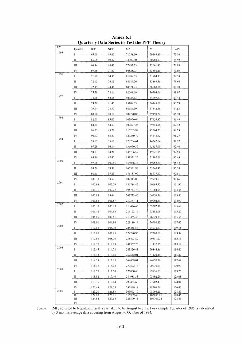
- 60 -

Annex 6.1 Quarterly Data Series to Test the PPP Theory

FY Quarter ICPI NCPI M2 M1 IWPI

1995 I 65.08 69.63 71058.10 29168.80 73.16

II 65.68 69.32 74302.30 30903.73 74.92

III 66.44 68.42 77493.23 32061.43 76.83

IV 69.46 71.60 80825.93 33398.10 79.05 1996

I 71.88 74.87 81289.03 31984.13 79.53

II 72.03 74.15 84684.26 33863.56 79.64

III 72.49 74.44 88821.73 36088.80 80.10

IV 75.59 78.16 92004.69 36794.06 81.97 1997

I 78.08 82.35 92326.13 34797.33 83.44

II 79.29 81.46 95109.33 36145.60 83.73

III 79.74 78.70 98686.39 37842.36 84.53

IV 80.50 80.10 102770.86 39190.22 85.70 1998

I 82.01 85.00 103990.64 37659.87 86.49

II 84.81 84.63 109827.25 39513.78 87.42

III 86.55 85.71 116203.99 42564.25 88.29

IV 90.63 88.87 123280.72 44448.32 91.27 1999

I 95.69 95.60 128704.61 44247.64 92.27

II 97.28 96.14 136070.37 45657.00 92.40

III 94.03 94.21 145706.59 49521.75 92.53

IV 95.46 97.42 151331.25 51497.68 93.49 2000

I 97.66 100.65 154088.38 49952.51 95.12

II 98.26 99.38 165391.99 55540.42 95.38

III 98.41 97.83 176187.90 58777.47 97.81

IV 100.30 98.52 182343.00 59778.63 99.66 2001

I 100.98 102.29 186784.42 60665.32 101.90

II 101.36 102.22 195744.78 63604.94 103.34

III 100.98 99.64 203773.46 66956.16 103.86

IV 103.63 101.87 210367.11 69992.31 104.97 2002

I 105.37 105.23 213426.43 69382.16 105.62

II 106.42 104.98 219122.19 73182.09 105.27

III 106.05 102.61 219455.43 76029.37 105.58

IV 108.01 104.96 221189.19 76980.13 107.47 2003

I 110.05 108.90 225455.54 74738.77 109.16

II 110.05 107.85 229790.95 77380.01 109.34

III 110.66 108.76 235423.87 79311.23 112.16

IV 112.77 112.09 241357.26 81437.75 113.12 2004

I 113.45 114.78 243826.43 79344.86 114.40

II 114.13 113.48 252642.01 81420.14 115.82

III 114.29 112.65 264459.01 86970.56 117.69

IV 116.18 114.02 270822.13 90070.71 120.93 2005

I 118.75 117.70 277060.40 89936.03 123.27

II 118.82 117.40 284988.33 93492.20 123.08

III 119.35 119.14 290453.63 97782.43 124.04

IV 120.48 121.35 295899.18 98596.26 126.45 2006 I 123.20 126.83 303673.19 98096.25 128.49

II 124.87 126.91 315909.48 102853.61 128.45 III 124.84 127.64 325899.15 106701.24 128.41 IV

Source: IMF, adjusted to Nepalese Fiscal Year taken to be August to July. For example I quarter of 1995 is calculated by 3 months average data covering from August to October of 1994.

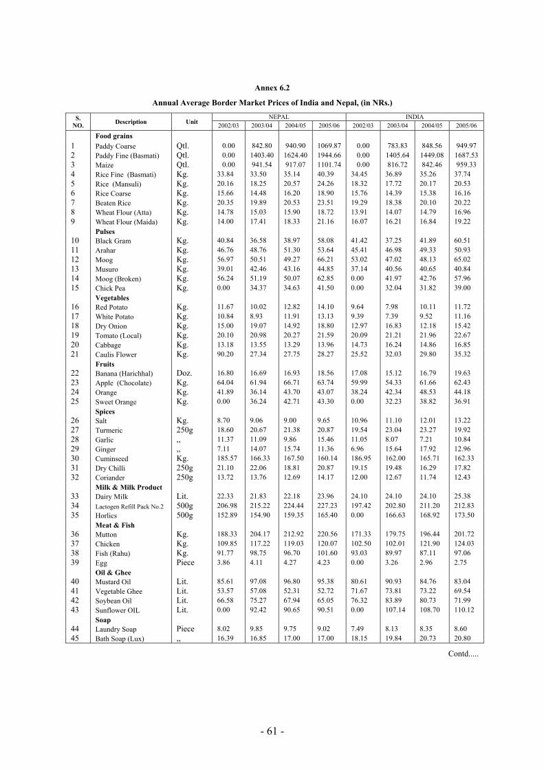
- 61 -

Annex 6.2

Annual Average Border Market Prices of India and Nepal, (in NRs.)

S. NO. Description Unit

NEPAL INDIA 2002/03 2003/04 2004/05 2005/06 2002/03 2003/04 2004/05 2005/06

Food grains

1 Paddy Coarse Qtl. 0.00 842.80 940.90 1069.87 0.00 783.83 848.56 949.97 2 Paddy Fine (Basmati) Qtl. 0.00 1403.40 1624.40 1944.66 0.00 1405.64 1449.08 1687.53 3 Maize Qtl. 0.00 941.54 917.07 1101.74 0.00 816.72 842.46 959.33 4 Rice Fine (Basmati) Kg. 33.84 33.50 35.14 40.39 34.45 36.89 35.26 37.74 5 Rice (Mansuli) Kg. 20.16 18.25 20.57 24.26 18.32 17.72 20.17 20.53 6 Rice Coarse Kg. 15.66 14.48 16.20 18.90 15.76 14.39 15.38 16.16 7 Beaten Rice Kg. 20.35 19.89 20.53 23.51 19.29 18.38 20.10 20.22 8 Wheat Flour (Atta) Kg. 14.78 15.03 15.90 18.72 13.91 14.07 14.79 16.96 9 Wheat Flour (Maida) Kg. 14.00 17.41 18.33 21.16 16.07 16.21 16.84 19.22 Pulses 10 Black Gram Kg. 40.84 36.58 38.97 58.08 41.42 37.25 41.89 60.51 11 Arahar Kg. 46.76 48.76 51.30 53.64 45.41 46.98 49.33 50.93 12 Moog Kg. 56.97 50.51 49.27 66.21 53.02 47.02 48.13 65.02 13 Musuro Kg. 39.01 42.46 43.16 44.85 37.14 40.56 40.65 40.84 14 Moog (Broken) Kg. 56.24 51.19 50.07 62.85 0.00 41.97 42.76 57.96 15 Chick Pea Kg. 0.00 34.37 34.63 41.50 0.00 32.04 31.82 39.00 Vegetables 16 Red Potato Kg. 11.67 10.02 12.82 14.10 9.64 7.98 10.11 11.72 17 White Potato Kg. 10.84 8.93 11.91 13.13 9.39 7.39 9.52 11.16 18 Dry Onion Kg. 15.00 19.07 14.92 18.80 12.97 16.83 12.18 15.42 19 Tomato (Local) Kg. 20.10 20.98 20.27 21.59 20.09 21.21 21.96 22.67 20 Cabbage Kg. 13.18 13.55 13.29 13.96 14.73 16.24 14.86 16.85 21 Caulis Flower Kg. 90.20 27.34 27.75 28.27 25.52 32.03 29.80 35.32 Fruits 22 Banana (Harichhal) Doz. 16.80 16.69 16.93 18.56 17.08 15.12 16.79 19.63 23 Apple (Chocolate) Kg. 64.04 61.94 66.71 63.74 59.99 54.33 61.66 62.43 24 Orange Kg. 41.89 36.14 43.70 43.07 38.24 42.34 48.53 44.18 25 Sweet Orange Kg. 0.00 36.24 42.71 43.30 0.00 32.23 38.82 36.91 Spices 26 Salt Kg. 8.70 9.06 9.00 9.65 10.96 11.10 12.01 13.22 27 Turmeric 250g 18.60 20.67 21.38 20.87 19.54 23.04 23.27 19.92 28 Garlic ,, 11.37 11.09 9.86 15.46 11.05 8.07 7.21 10.84 29 Ginger ,, 7.11 14.07 15.74 11.36 6.96 15.64 17.92 12.96 30 Cuminseed Kg. 185.57 166.33 167.50 160.14 186.95 162.00 165.71 162.33 31 Dry Chilli 250g 21.10 22.06 18.81 20.87 19.15 19.48 16.29 17.82 32 Coriander 250g 13.72 13.76 12.69 14.17 12.00 12.67 11.74 12.43 Milk & Milk Product 33 Dairy Milk Lit. 22.33 21.83 22.18 23.96 24.10 24.10 24.10 25.38 34 Lactogen Refill Pack No.2 500g 206.98 215.22 224.44 227.23 197.42 202.80 211.20 212.83 35 Horlics 500g 152.89 154.90 159.35 165.40 0.00 166.63 168.92 173.50 Meat & Fish 36 Mutton Kg. 188.33 204.17 212.92 220.56 171.33 179.75 196.44 201.72 37 Chicken Kg. 109.85 117.22 119.03 120.07 102.50 102.01 121.90 124.03 38 Fish (Rahu) Kg. 91.77 98.75 96.70 101.60 93.03 89.97 87.11 97.06 39 Egg Piece 3.86 4.11 4.27 4.23 0.00 3.26 2.96 2.75 Oil & Ghee 40 Mustard Oil Lit. 85.61 97.08 96.80 95.38 80.61 90.93 84.76 83.04 41 Vegetable Ghee Lit. 53.57 57.08 52.31 52.72 71.67 73.81 73.22 69.54 42 Soybean Oil Lit. 66.58 75.27 67.94 65.05 76.32 83.89 80.73 71.99 43 Sunflower OIL Lit. 0.00 92.42 90.65 90.51 0.00 107.14 108.70 110.12 Soap 44 Laundry Soap Piece 8.02 9.85 9.75 9.02 7.49 8.13 8.35 8.60 45 Bath Soap (Lux) ,, 16.39 16.85 17.00 17.00 18.15 19.84 20.73 20.80

Contd.....

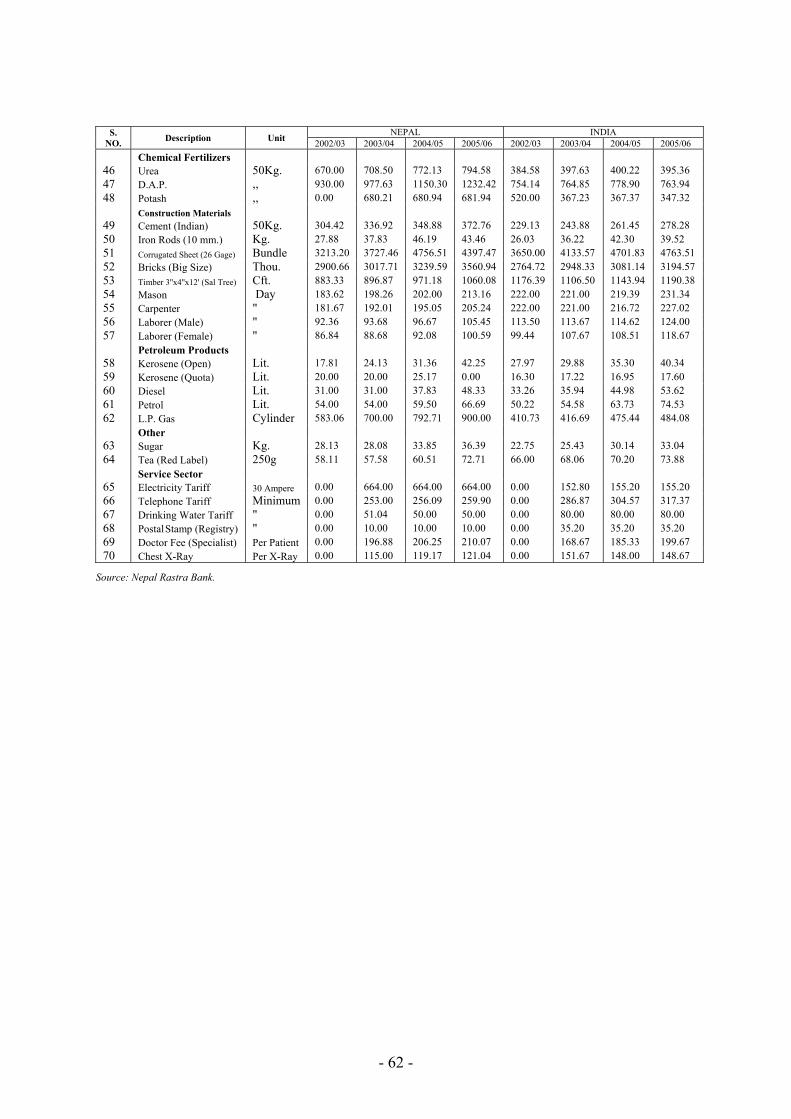
- 62 -

S.

NO. Description Unit NEPAL INDIA 2002/03 2003/04 2004/05 2005/06 2002/03 2003/04 2004/05 2005/06

Chemical Fertilizers 46 Urea 50Kg. 670.00 708.50 772.13 794.58 384.58 397.63 400.22 395.36 47 D.A.P. ,, 930.00 977.63 1150.30 1232.42 754.14 764.85 778.90 763.94 48 Potash ,, 0.00 680.21 680.94 681.94 520.00 367.23 367.37 347.32 Construction Materials 49 Cement (Indian) 50Kg. 304.42 336.92 348.88 372.76 229.13 243.88 261.45 278.28 50 Iron Rods (10 mm.) Kg. 27.88 37.83 46.19 43.46 26.03 36.22 42.30 39.52 51 Corrugated Sheet (26 Gage) Bundle 3213.20 3727.46 4756.51 4397.47 3650.00 4133.57 4701.83 4763.51 52 Bricks (Big Size) Thou. 2900.66 3017.71 3239.59 3560.94 2764.72 2948.33 3081.14 3194.57 53 Timber 3''x4''x12' (Sal Tree) Cft. 883.33 896.87 971.18 1060.08 1176.39 1106.50 1143.94 1190.38 54 Mason Day 183.62 198.26 202.00 213.16 222.00 221.00 219.39 231.34 55 Carpenter " 181.67 192.01 195.05 205.24 222.00 221.00 216.72 227.02 56 Laborer (Male) " 92.36 93.68 96.67 105.45 113.50 113.67 114.62 124.00 57 Laborer (Female) " 86.84 88.68 92.08 100.59 99.44 107.67 108.51 118.67 Petroleum Products 58 Kerosene (Open) Lit. 17.81 24.13 31.36 42.25 27.97 29.88 35.30 40.34 59 Kerosene (Quota) Lit. 20.00 20.00 25.17 0.00 16.30 17.22 16.95 17.60 60 Diesel Lit. 31.00 31.00 37.83 48.33 33.26 35.94 44.98 53.62 61 Petrol Lit. 54.00 54.00 59.50 66.69 50.22 54.58 63.73 74.53 62 L.P. Gas Cylinder 583.06 700.00 792.71 900.00 410.73 416.69 475.44 484.08 Other 63 Sugar Kg. 28.13 28.08 33.85 36.39 22.75 25.43 30.14 33.04 64 Tea (Red Label) 250g 58.11 57.58 60.51 72.71 66.00 68.06 70.20 73.88 Service Sector 65 Electricity Tariff 30 Ampere 0.00 664.00 664.00 664.00 0.00 152.80 155.20 155.20 66 Telephone Tariff Minimum 0.00 253.00 256.09 259.90 0.00 286.87 304.57 317.37 67 Drinking Water Tariff " 0.00 51.04 50.00 50.00 0.00 80.00 80.00 80.00 68 Postal Stamp (Registry) " 0.00 10.00 10.00 10.00 0.00 35.20 35.20 35.20 69 Doctor Fee (Specialist) Per Patient 0.00 196.88 206.25 210.07 0.00 168.67 185.33 199.67 70 Chest X-Ray Per X-Ray 0.00 115.00 119.17 121.04 0.00 151.67 148.00 148.67

Source: Nepal Rastra Bank.

- 63 -

Annex 6.3

Some Comments on "Inflation in Nepal"

(a) Comments on the study “Inflation in Nepal, 2007” by Prof. Dr. Gunanidhi Sharma35 Nepal Rastra Bank (NRB) as a monetary authority in Nepal needs to be understood as

a part of national economy and society, as its object is to keep economy and, hence, the society in order. It is two in one. While it, on the one hand, works as a regulatory authority, its role as a development authority, on the other, is equally important in the country like Nepal, which is facing the challenges of the development of under development. The challenges of underdevelopment appear when the economy and society here are interlocked the way that slow pace of transformation of one is automatically manifested into the other. The role of the NRB, thus, must be taken for granted as the causal factor to shape the society in Nepal as wished by the Interim Constitution, 2063, which emphatically aims at realizing distributive justice. In this sense, the role of the NRB is expanding with the growth of Nepalese society by all account. The NRB is undertaking diverse activities in the sequence and the study on inflation in Nepal under consideration is a by-product of its activities as an apex bank or a financial institution.

The study is impressive in the sense that it is systematic, comprehensive, scholarly and rigorous. In an attempt to shorting out issues of inflation in Nepal, it digs out the historical facts, relationships, NRB attempts and price behavior in monetary sector of the Nepalese economy applying standard latest more reliable econometric tools. It tries to answer: How is inflation determined in Nepal? The purpose of the study, however, is to explore, through an in-depth analysis and the empirical verification, the possibility of realizing economic and financial stability using monetary management techniques. Meanwhile, it is conscious about the policy constraints or contradictions inherent in the structure of the Nepalese economy, whether they are man made, culturally affixed, or geographically attributed.

The study begins with the conviction that inflation is a public concern that needs shaping (streamlining) in the interest of all poor and rich, producers and consumers, savers and investors, borrowers and lenders, etc. Also, it tries to account the complexities in state management working for public welfare and fighting with illegal and underworld activities but giving high and phenomenal importance to the appropriate level of prices in the interest of all economic agents who wish the inflation to be contained within acceptable limit.

Of course, state management in Nepal is a complex business. Mainly, it is so for its external relations shaped by its history, geography and culture. These factors are the conclusions derived under various treaties including the ones in 1950 with India by way of which Nepal was compelled to accept the 'neighborhood economy' principle. It has put Nepal under vulnerable position in that the economic and social problems here get never matured and hence they are made chronic. Its ultimate demerit is the situation when state is never serious about national self-reliance.

Specially, Nepal for its 1950 treaties with India loses its ground for policy regulations concerned with the activities of trade, investment, labor, fiscal and financial exercises, foreign exchange flows, savings, and so on. Consequently, Nepal historically is deprived of economic and social independence the manifestation of which is

35 Professor Sharma is currently affiliated with Central Department of Economics, Tribhuwan University, Nepal.

- 64 -

underlined by its incapability of keeping big economic indicators like prices, money supply, interest rates, etc., in its own favor; although consolation for Nepal is the role played by Indian economy working as the stabilizing factor in Nepal. Since the stability touches its bottom line of stagnancy, roaming around Hindu Growth rate of almost three percent per annum at all times Nepal could never materialize the dream of emancipating the country from economic depression, repression and deprivation. Vital issues for us, therefore, are of structural and institutional corrections rather than the fine-tuning of monetary policy. The study, even if less elaborative, seems serious when it reaches the historical conclusion that money supply effect on prices in Nepal is swamped by Indian price structure and opening of its capital account can make interest rates reshuffled against policy interest.

Overwhelmingly, the study is traditional in its perception about Nepalese inflation when it says: Low inflation is attributed to tight monetary policy (p.8), improvement in production is for correct public policy (p.8), etc. Statements are difficult to digest by the commonsense of an ordinary Nepali who is convinced that, nearly a failed state, this country is determined mostly structurally, institutionally and externally throughout its history. It means policies in Nepal face gaps historically. One should, therefore, understand that the efficacy of monetary policy here is a function not of tight or easy monetary policy (relying on quantitative method or credit control mainly after late 1980s) but of monetization of the vast (seventy-five percent) rural economy de-linked financially from urban and international centers. The rural area is suffering from economic isolation, inefficiency and fragmentation. The Maoist insurgency, which caused for either the withdrawal or the deprivation of organized financial activities in most part of the country poured fuel in the fire. Study statements are also not consistent with its own arguments in the text (p 16, pp.28-29) where it sensed inflation in Nepal is a social, institutional, cultural, economic and, in all, political (including relations with India) phenomenon.

The study, nevertheless, is correct in its outcome that Nepal's big challenge continuously lies in dependency syndrome and the consequence thereof. As it is importing more than seventy per cent of its essential supplies it also imports inflation from India in the same proportion. This fact is precisely underlined in the test results of the study where Indian inflation rather than the financial performance at home is the predominant factor in determining prices in Nepal (Chapter 6). Prices of wage goods, inadequate supply of services, cartelling and other bottlenecks as well on the supply side may be the not less significant sources (less seriously talked about in the study) of inflation in the country. The study is uniquely verifying Keynesian "supply responds hypothesis" and its subsequent post Keynesian thesis with the biasness towards demand management. Equations estimated, however, included explanatory variables representing both of the demand and supply sides. Hence, they are named of the hybrid form. Nevertheless, the text is silent, on the one hand, of the problem of identification that which side we are estimating the demand or supply, and whether equations are in reduced form, on the other. Conclusions in exact, however, are: "M1 has significant effect on inflation in first and second lags, but M2 has effect only in second lag" (p.33). Results are consistent with theories in that M1 is the transaction demand for money and time and part of the savings deposits in M2 are the basis of financial intermediation, and hence M2 mostly is investment made for earning rate of interest. Its impact may be on productivity (on the supply side) rather than on inflation.

- 65 -

The one for one correspondence between Indian and Nepalese prices (refer section 5.9 of Chapter 5 and the discussions of the "Law of One Price" in Chapter 6) are for:

1. Special relations between Nepal and India defined by the treaties of 1950 and the composition of imports from India in which more than seventy per cent of the total comprises essentials.

2. The officially pegged foreign exchange rate for NC and IC not only regulates prices of other currencies in the domestic market via IC - Dollar rate in Mumbai but also fully translates Indian prices into Nepalese prices. This implies exchange rate in Nepal is burden free and hence NRB must rely on foreign exchange reserve policy for keeping foreign relations in order. But since it cannot regulate supply of reserves it should concentrate on regulating their uses.

Apparently, indicator of monetary policy in the external front is foreign exchange reserves under pegged system. The change in reserves is translated into money supply with effect on prices. Since foreign exchange reserve is out of policy control, achieving price stability through changes in reserve base is highly unlikely.

Therefore, on the said grounds, it can be inferred that NRB's recent policy targeting price stability needs rethinking. The study also reaches the same conclusion when it says, "inflation target within the present domestic context may require more vigorous exercise to make (P.34)”. NRB, hence, must focus on "stability through growth rather than growth through stability". Accordingly, NRB must work with credit policy, which influences all three variables at a time, Say, growth, inflation and the rate of interest. Dynamics of economic adjustment in the initiation of NRB, thus, must undoubtedly be understood as the adjustment in economic structure via sectoral distribution of credits. This justifies the need of micro economic policy directed towards allocative efficiency and distributive justice.

Also, an additional but vital issue raised by the study is: Whether Nepalese economy is active or passive in terms of its functioning? If dominant market clearing forces determining the level of economic activities are generated or significantly influenced by forces outside the system, the economy is passive in responding to the policy changes. Even it if responds it is indirectly via the adjustment in foreign sector. Means, NRB policy should rely on its response to foreign shocks rather than the internal demand of the policy changes. It devises a system where the NRB is always dancing to the tune of external impulses attached with the flows of trade, aid and technology transfer. This converses the NRB status of development and regulatory authority into the feedback agency guided by the principle of "Your choice is my choice".

Above all, the study discovers pertinent inherent issues relating to the movement of prices in Nepal. Conclusions are derived, accordingly, from the estimation of price equations applying rigorous econometric tools, theoretical reasoning, institutional judgments and commonsense. The study may be a landmark for future research on Inflation in Nepal. Policy makers, academicians and social scientists can be benefited from its scientific approach, generalizations and organizations.

Thank you.

- 66 -

(b) Some comments on the paper “Inflation in Nepal” by Dr. Shankar Sharma36

First of all I would like to thank Nepal Rastra Bank, Research Department, Price Division for providing me the opportunity to participate in this workshop and present my comments on the paper "Inflation in Nepal", a topic of growing importance, prepared by the Division. I would like to focus my comments on the greater economic integration between Nepal and India and its potential influence on inflation and the associated implications for modeling the price movements.

The study reviews theories of inflation, presents literature review, examines the trend of inflation in Nepal, identifies the short-term and long-term relationship of inflation and analyses the impact of determining variables in inflation. The analysis concludes that inflation in Nepal is mainly determined by Indian inflation with narrow money only having an effect in the short run (less than one year).

The study attributed this relationship on the existing open border between Nepal and India, which facilitates informal trade and a rigid pegged exchange rate regime between both currencies along with varying capital mobility. As the main influencing factor of inflation in Nepal are the pegged exchange rate and capital mobility between the two countries, NRB could control the domestic inflation only in the short run (1 year window) but will have limited control beyond that.

The analysis done in the paper is comprehensive. However, one can ask a number of questions with regard to conclusions, policy perspectives and modeling. They are:

• What are the impacts of the price movements of non-tradable on inflation?

• What is the role of imports from third countries (other than that of India) on Nepalese inflation?

• How can we predict inflation in Nepal?

• What do we do if the rising inflation trend is observed in India?

• What are some of the structural issues that can help explain inflation in Nepal, so that the government and private sectors can prepare themselves to minimize the adverse impact of price movements in India on the production and productivity of goods and services in Nepal?

There are a number of goods and services included in estimating the CPI in Nepal, which are to a large extent non-tradable in nature. As for example, how restaurant meals and local production (e.g. milk and milk products and vegetables) that are probably least affected by Indian imports and production capacity, can affect inflation in Nepal. Similarly, what will be the impact of wage cost, housing, transportation and communication costs, medical and personal care and educational costs on domestic inflation? How do we explain it?

Nepal imports about one-third of its total imports from third countries. How this will affect the inflation in Nepal? What will be the impact of globalization on inflation? If it influences through Indian market, what is the mechanism?

How can we predict inflation rate, if the domestic parameters cannot be used to predict it? How can we keep the inflation rate in a desired level? The standard model will have difficulty in answering the question.

36 Dr. Sharma is former vice chairman of National Planning Commission, Government of Nepal.

- 67 -

Now, I would like to comment on the modeling aspects of inflation from policy perspectives.

Of course, the integration of the product and financial markets has been established between Nepal and India since long. However, the share of Nepalese trade with India (measured by nominal exports plus imports as a share of nominal gross domestic product), which declined after 1990, has been rising again especially after 1996. The main reasons for increasing trade between the two countries are the trade agreement carried out between Nepal and India in 1996, which allowed exports of almost all Nepali manufacturing products to India, duty free and quota free and the liberalization of Indian economy. Liberalization of Indian economy, which helped to increase the productivity of Indian economy, also facilitated increase of Indian imports in Nepal, considerably.

It is not only between Nepal and India, globalization has also changed global inflationary phenomenon noticeably. I would like to, first draw parallel between the global inflationary phenomenon and the one that we have observed in Nepal.

Even if inflation is largely a monetary phenomenon the opening up of China and India, in particular, has resulted on the dis-inflationary effect, worldwide. Huge increase in the global supply of mainly lower-skilled workers, due to liberalization has resulted in low cost of production in these and other emerging economies and has led to a geographic shift in production toward them-not just from the developed countries but also from other formerly low-cost producers such as Mexico, Korea, Singapore and Taiwan.

This has concluded that the inflation is not only domestic 'demand pull' or 'cost push' phenomenon, but also determined by foreign production and demand conditions. This implies that inflation perhaps has become less sensitive to domestic demand conditions. However, the extent of this shift on inflation is less obvious. This is also a research question.

On the other hand, globalization can also exert downward pressure on domestic wage growth, restrain labor costs and increase productivity (could accelerate division of labor in production and encourage exploitation of comparative advantages of the countries even further).

In trying to assess and explain movements in inflation, which are affected by economic integration between Nepal and India, reduced form equation probably is better.

Using this framework, one can look for the effect of greater integration in several ways. First, the model, directly can examine the influence of import prices (and therefore trade flows) on domestic inflation. Second, we can look for evidence of integration-related structural change in the model by examining the stability of the parameter estimates.

Third, we can see whether we have omitted from the standard model any variables that might be interpreted as representing changes in globalization. And, finally, we can look for evidence of model errors that would be consistent with the hypothesis that globalization has been restraining inflation.

The analysis can also say something about the production capacity of Nepal. If the influence of Indian inflation is high on Nepalese domestic prices, increases in Indian

- 68 -

production capacity, in recent years could have limited the ability of Nepalese producers to raise prices in response to increases in the domestic costs of production, if any. This will also have serious implications to the industrialization process in Nepal. In the context of the inflation model, we also need to examine this issue.

Greater integration between the two countries could also have either restrained unit labor costs in Nepal by raising productivity or increased unit labor costs without any gain in the productivity of the economy. Increasing volumes of trade should boost productivity as economies concentrate their resources in those sectors in which they are relatively more efficient. But it is difficult to observe evidence to which grater economic integration between Nepal and India may have boosted aggregate productivity growth in Nepal.

These observations bring to me to the final point, which is about monetary policy. Clearly, just like the greater integration of the world's economies does leave the many countries of the world more open to influences from abroad, greater economic integration with India results excesses or shortfalls in demand in Nepal to be absorbed by India through adjustments of our imports and exports.

But we are also subject to higher inflationary forces from India. In this situation, how can the monetary policy maximize its role in dampening the inflationary pressure in Nepal? What are some of the other policy issues, which can create the resilience from the Indian inflationary pressure? How Indian production capacity and unit labor costs and other structural changes influence Nepalese inflation and production capacity? These are some of the question, which can have major policy implications, probably can be better answered by reduced form equations. These are some of the research questions for the future studies.

Thank you.