March 2003 • NREL/CP-550-33698

Infiltration and Natural Ventilation Model for Whole-Building Energy Simulation of Residential Buildings

Preprint

M. Deru National Renewable Energy Laboratory

P. Burns Colorado State University

To be presented at the ASHRAE Conference Kansas City, Missouri June 28–July 2, 2003

National Renewable Energy Laboratory 1617 Cole Boulevard Golden, Colorado 80401-3393 NREL is a U.S. Department of Energy LaboratoryOperated by Midwest Research Institute • Battelle • Bechtel

Contract No. DE-AC36-99-GO10337

NOTICE The submitted manuscript has been offered by an employee of the Midwest Research Institute (MRI), a contractor of the US Government under Contract No. DE-AC36-99GO10337. Accordingly, the US Government and MRI retain a nonexclusive royalty-free license to publish or reproduce the published form of this contribution, or allow others to do so, for US Government purposes.

This report was prepared as an account of work sponsored by an agency of the United States government. Neither the United States government nor any agency thereof, nor any of their employees, makes any warranty, express or implied, or assumes any legal liability or responsibility for the accuracy, completeness, or usefulness of any information, apparatus, product, or process disclosed, or represents that its use would not infringe privately owned rights. Reference herein to any specific commercial product, process, or service by trade name, trademark, manufacturer, or otherwise does not necessarily constitute or imply its endorsement, recommendation, or favoring by the United States government or any agency thereof. The views and opinions of authors expressed herein do not necessarily state or reflect those of the United States government or any agency thereof.

Available electronically at http://www.osti.gov/bridge

Available for a processing fee to U.S. Department of Energy and its contractors, in paper, from:

U.S. Department of Energy Office of Scientific and Technical Information P.O. Box 62 Oak Ridge, TN 37831-0062 phone: 865.576.8401 fax: 865.576.5728 email: reports@adonis.osti.gov

Available for sale to the public, in paper, from: U.S. Department of Commerce National Technical Information Service 5285 Port Royal Road Springfield, VA 22161 phone: 800.553.6847 fax: 703.605.6900 email: orders@ntis.fedworld.gov online ordering: http://www.ntis.gov/ordering.htm

Printed on paper containing at least 50% wastepaper, including 20% postconsumer waste

Tables of Contents

Nomenclature .................................................................................................................................................... iiAbstract ............................................................................................................................................................. 1Introduction....................................................................................................................................................... 1Theoretical Formulation.................................................................................................................................... 2

Stack Pressures.............................................................................................................................................. 2Wind Pressures.............................................................................................................................................. 3Total Pressure Difference.............................................................................................................................. 5

Mass-flow Rate Equations ................................................................................................................................ 6Infiltration/Exfiltration.................................................................................................................................. 6Natural Ventilation........................................................................................................................................ 7Mechanical Ventilation ................................................................................................................................. 7

Solution Techniques.......................................................................................................................................... 8Newton-Raphson Method ............................................................................................................................. 8Convergence.................................................................................................................................................. 9

Verification and Validation............................................................................................................................. 10Analytical Verification................................................................................................................................ 10Comparison of the Infiltration Model ......................................................................................................... 10Comparison of Natural Ventilation Model.................................................................................................. 14

Summary ......................................................................................................................................................... 16References....................................................................................................................................................... 16

List of Figures

Figure 1. Stack pressure across a wall with the inside warmer than the outside............................................... 3Figure 2. Surface pressure coefficient as a function of wind incident angle for the Walton model and the

Swami and Chandra model for side ratios S = L1/L2................................................................................. 4Figure 3. Comparison of SUNREL with the LBL infiltration model for stack effect..................................... 11Figure 4. Comparison of SUNREL and the LBL model for wind effect and no leakage in the roof or floor. 12Figure 5. Comparison of SUNREL and the LBL model for wind effect and 25% of the leakage in the roof

and 25% in the floor................................................................................................................................ 13Figure 6. Comparison of SUNREL and the LBL model for both stack and wind effects............................... 13Figure 7. Comparison of the natural ventilation model for the outbuilding with different values of the flow

exponent, n .............................................................................................................................................. 15Figure 8. Comparison of the natural ventilation model for the laboratory with different values for the flow

exponent, n .............................................................................................................................................. 15

List of Tables

Table 1. Parameters for Standard Terrain Classifications................................................................................. 5Table 2. Local Shielding Parameters ................................................................................................................ 5Table 3. Infiltration and Natural Ventilation Parameters for Analytical Testing............................................ 10Table 4. Infiltration and Natural Ventilation Parameters for Analytical Testing............................................ 14

i

Nomenclature A area (m2, ft2) ACH air changes per hour c pressure adjustment term from Newton’s method C combined flow coefficient from a blower door test CD discharge coefficient CP average surface pressure coefficient CP ′ pressure coefficient normalized to the pressure coefficient at normal incidence C1, C2, C3 infiltration coefficients ELA effective leakage area (cm2, in2) f fraction of the zone ELA in the wall G natural log of the side ratio (ratio of the lengths of adjacent building sides) g acceleration of gravity (m/s2, ft/s2)H height (m, ft) J Jacobian matrix L length of a building exterior surface (m, ft) &m mass-flow rate (kg/s, lbm/s) &m vector of building mass-flow rate (kg/s, lbm/s)

M constant multiplier for infiltration calculations n flow exponent P pressure (Pa, lbf/ft2) Po base pressure (at y = 0) in a zone (Pa, lbf/ft2) ∆P pressure difference from inside to outside across a wall (Pa, lbf/ft2) ∆Ps,o stack pressure difference at the base of a wall (Pa, lbf/ft2) ∆Ps,H stack pressure difference at the top of a wall (Pa, lbf/ft2) Q volumetric infiltration flow rate (m3/s, ft3/s) S side ratio (ratio of the lengths of adjacent building sides) SC normalized shielding coefficient T temperature (°C, °F) V speed (m/s, ft/s) y height above the bottom of the zone (m, ft) y’ height above the bottom of the zone normalized to the zone height α terrain dependent parameter for power law expression of wind speed β infiltration relaxation coefficient adjustment parameter or surface tilt γ terrain dependent parameter for power law expression of wind speed γs surface azimuth angle (south = 0 deg, east is negative and west is positive) ε infiltration convergence tolerance λ convergence speed multiplier ξ speed of convergence (fraction) ρ air density (kg/m3, lbm/ft3) ϕ wind incidence angle (deg) ψ wind direction from the weather file (north = 0 deg, east = 90 deg,, south = 180 deg.) ω relaxation coefficient

Subscripts e effective exf exfiltration H at the top of the surface of height in inside conditions inf infiltration

ii

min minimum met meteorological conditions npl neutral pressure level out outside or ambient conditions s stack effect tot total w wind

Superscripts k iteration number

iii

Abstract The infiltration term in the building energy balance equation is one of the least understood and most difficult to model. For many residential buildings, which have an energy performance dominated by the envelope, it can be one of the most important terms. There are numerous airflow models; however, these are not combined with whole-building energy simulation programs that are in common use in North America. This paper describes a simple multizone nodal airflow model integrated with the SUNREL whole-building energy simulation program. The required inputs for infiltration are taken from blower door test results and the geometry of the openings for natural ventilation. The flow exponents and coefficients for infiltration and natural ventilation can be input or left to the default values. Control of the natural ventilation openings can be controlled with a time scheduled and the indoor/outdoor temperature difference.

The mass-flow rate equations are written in terms of the pressure at the base of each zone. The pressure on each surface is a combination of stack and wind effects added to the zone base pressure. The resulting set of mass balance equations are solved using a Newton-Raphson iterative method with a variable relaxation coefficient. The relaxation coefficient is adjusted each iteration depending on the speed of the convergence. The iterations are stopped when the mass balance in each zone converges to a specified tolerance. The model exhibits good numerical behavior, with no singularities and only a few instances of nonconvergence in some building simulations with no thermal mass and large leakage areas. The infiltration model compares favorably to the LBL infiltration model. The natural ventilation model also compares well with another natural ventilation model and with measured results. The current infiltration model and whole-building simulation program form the basis of a new residential energy-auditing tool.

Introduction This paper presents a multizone infiltration/natural ventilation model that is simple, flexible, and driven by weather conditions. This model was added to the SERI-RES version 1.0 (SERI-RES 1988) whole-building energy simulation program as part of work to upgrade the program to a new version called SUNREL (Deru et al. 2002). The model is verified with analytic calculations and compared with other infiltration and natural ventilation models.

There have been numerous building airflow models developed; a survey by Feustel and Dieris (1992) reviewed 50 models. The most recognized single-zone model is the LBL model (Sherman and Grimsrud 1980, Sherman and Modera 1986), which has been extensively verified with measured data. The most widely recognized multizone models in the United States are CONTAM (Dols 2001; Dols and Walton 2002) and COMIS (Feustel and Rayner-Hooson 1990, Feustel 1999). Both of these programs were designed to be used as stand-alone programs; however, these programs can also be combined with building energy simulation programs. Kendrick (1993) reviewed such coupling strategies and surveyed nine programs. COMIS has recently been used in combination with a whole-building energy simulation program (Huang et al. 1999). Another stand-alone model that has been integrated into a whole-building energy simulation program is MIX (Li et al. 2000).

Most whole-building energy simulation programs have very simplified infiltration models because it is usually a small load in large buildings. However, for small buildings, infiltration can be one of the most important terms in the energy balance equation, and it is one of the most difficult to model accurately. One of the difficulties in simulating infiltration is relating physical measurements of the leakage to a mathematical model. Ideally, the size, location, and characteristics of all leakage areas in the building should be known; however, this information is impossible to quantify. The most common measurement technique for infiltration in small buildings is the blower door test. This method is simple and results in an approximation of the effective leakage area (ELA), but it yields very little information concerning the geometry or spatial distribution of the cracks. Another major obstacle is modeling the pressure distribution

1

due to the wind. The wind pressure distribution on the exterior of a building envelope is normally modeled with approximate correlations derived from physical measurements. With these uncertainties, it is nearly impossible to deduce accurate values of the instantaneous infiltration; however, over a longer period, it is possible to approximate the average effects of infiltration.

Natural ventilation is often an important method of controlling the thermal comfort in small buildings, and it is driven by the same fundamental mechanisms as infiltration. However, the problem of flow through large openings is more complex. For openings in exterior surfaces, wind turbulence can cause fluctuating flows especially for single-sided ventilation and when the wind is parallel to openings on opposite surfaces. For openings in interior surfaces, different density stratification in adjoining zones can bring about two neutral pressure levels within the opening and boundary layer effects introduce a different driving force (Feustel and Rayner-Hooson 1990). A simple model is developed here following the infiltration model that is limited to openings in vertical exterior surfaces and should not be used for single-sided ventilation.

Theoretical Formulation In SERI-RES, infiltration is modeled either as a fixed air change per hour (ACH) or by the polynomial of Eq. (1). The only control the user has with Eq. (1) is the user-defined multiplier M. The wind speed is Vwind, Tin and Tout are temperatures, and C1, C2, and C3 are constants. Neither of these methods are directly related to the physical dimensions or the leakage distribution in the building. In addition, the fixed ACH method does not vary with weather, and the method of Eq. (1) is a poor model of the dynamic interaction of the building and its environment.

ACH = M[C1 + C2Vwind + C3 (Tin − Tout )] (1)

The driving force for infiltration and exfiltration is the pressure difference across the building envelope. This pressure difference is a result of temperature differences between the inside and outside, wind pressures on the exterior surfaces, and mechanical sources of pressure such as fans. Only the pressures from temperature and wind effects are considered here because SUNREL does not model fan pressures. The basis for the discussion of the stack and wind pressures in the following two sections is not new; there are many excellent sources of information such as the ASHRAE Handbook of Fundamentals 2001 (ASHRAE 2001).

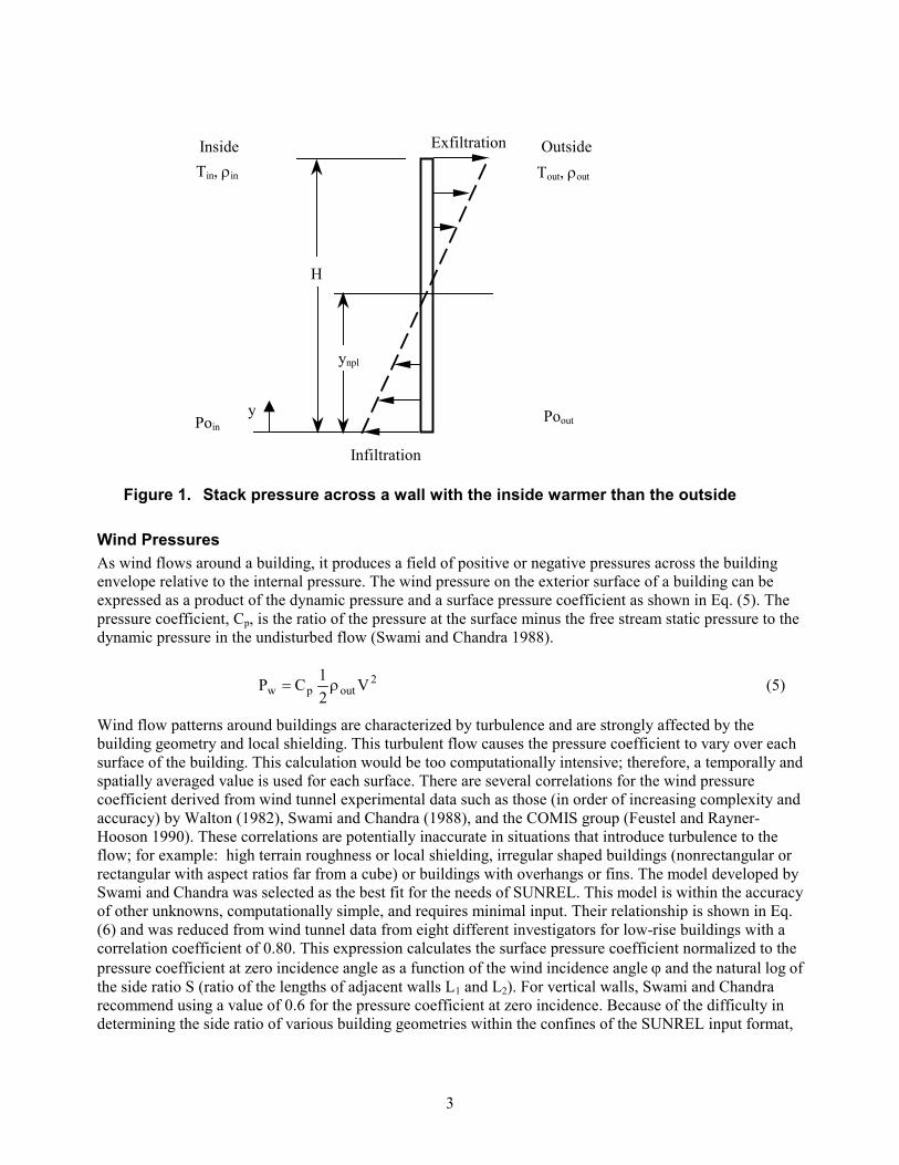
Stack Pressures The stack effect is produced by density differences due to the variation in temperature between inside and outside air. This variation in densities produces buoyancy forces, which drive the flow as shown in Figure 1. The height at which the pressures on both sides of the wall are equal is called the neutral pressure level ynpl. Assuming that the air on each side of the wall is well mixed, the pressure can be calculated as a function of height from the hydrostatic relation of Eq. (2). The pressure at the base of the wall is Po and is used as the reference pressure for the zone. The stack effect pressure difference across the wall as a function of the normalized height y’ is calculated by Eq. (3). Pressures are usually measured against a reference pressure, which is taken as the ambient base pressure Poout in this case. For convenience, this pressure is set to zero. The stack pressure difference can also be represented as Eq. (4), where ∆Ps,o is the stack pressure difference at the bottom of the wall and ∆Ps,H is the stack pressure difference at the top of the wall of height H.

Pin (y) = Poin − ρin gy (2)

∆Ps (y′) = Pin − Pout = (Poin − Poout ) − gHy′(ρin − ρout ) (3)

∆Ps (y′) = Poin − ∆Ps,o − y′∆Ps,H (4)

2

Inside Exfiltration Outside Tin, ρin

H

ynpl

y

Tout, ρout

Poin Poout

Infiltration

Figure 1. Stack pressure across a wall with the inside warmer than the outside

Wind Pressures As wind flows around a building, it produces a field of positive or negative pressures across the building envelope relative to the internal pressure. The wind pressure on the exterior surface of a building can be expressed as a product of the dynamic pressure and a surface pressure coefficient as shown in Eq. (5). The pressure coefficient, Cp, is the ratio of the pressure at the surface minus the free stream static pressure to the dynamic pressure in the undisturbed flow (Swami and Chandra 1988).

1 2 (5)Pw = Cp 2 ρout V

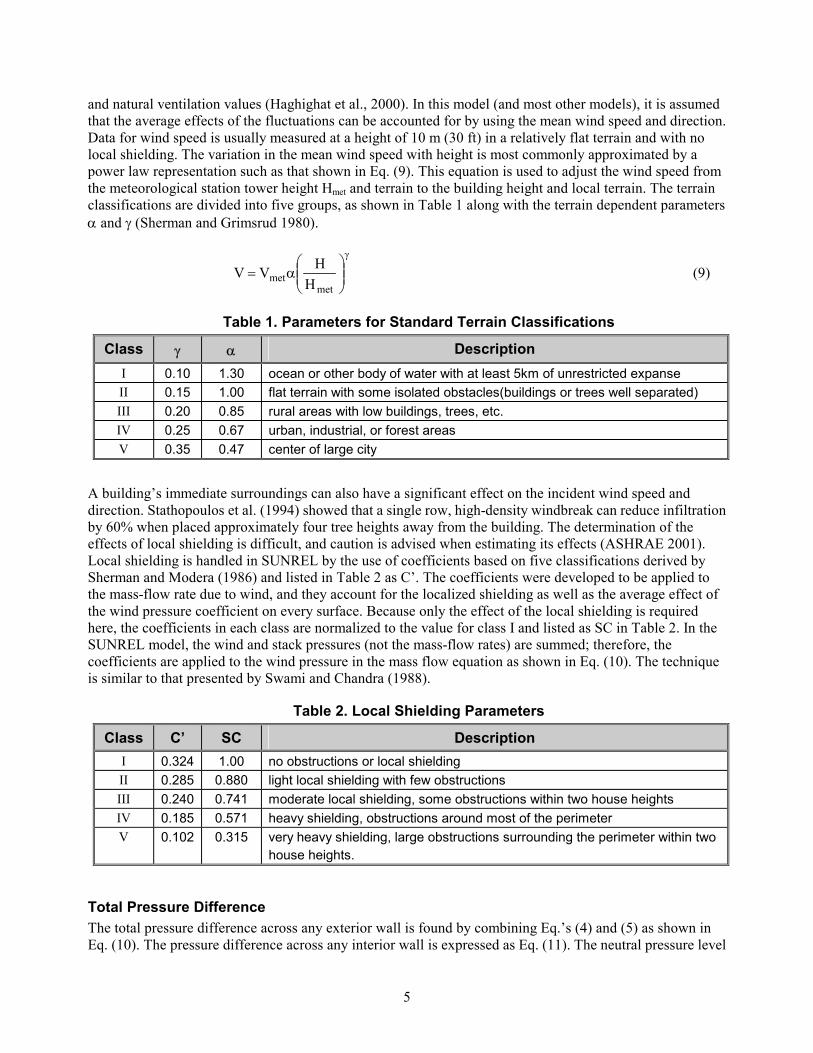
Wind flow patterns around buildings are characterized by turbulence and are strongly affected by the building geometry and local shielding. This turbulent flow causes the pressure coefficient to vary over each surface of the building. This calculation would be too computationally intensive; therefore, a temporally and spatially averaged value is used for each surface. There are several correlations for the wind pressure coefficient derived from wind tunnel experimental data such as those (in order of increasing complexity and accuracy) by Walton (1982), Swami and Chandra (1988), and the COMIS group (Feustel and Rayner-Hooson 1990). These correlations are potentially inaccurate in situations that introduce turbulence to the flow; for example: high terrain roughness or local shielding, irregular shaped buildings (nonrectangular or rectangular with aspect ratios far from a cube) or buildings with overhangs or fins. The model developed by Swami and Chandra was selected as the best fit for the needs of SUNREL. This model is within the accuracy of other unknowns, computationally simple, and requires minimal input. Their relationship is shown in Eq. (6) and was reduced from wind tunnel data from eight different investigators for low-rise buildings with a correlation coefficient of 0.80. This expression calculates the surface pressure coefficient normalized to the pressure coefficient at zero incidence angle as a function of the wind incidence angle ϕ and the natural log of the side ratio S (ratio of the lengths of adjacent walls L1 and L2). For vertical walls, Swami and Chandra recommend using a value of 0.6 for the pressure coefficient at zero incidence. Because of the difficulty in determining the side ratio of various building geometries within the confines of the SUNREL input format,

3

the side ratio is set to one. The error introduced by this is relatively small for most building geometries and incidence angles as shown in Figure 2 along with the correlation from Walton (1982).

C 1.248 − 0.703sin ϕ − 1.175sin 2 ϕ + 0.131sin3 (2ϕG) +

C′ = 2 p Cp (ϕ

p

= 0) = ln

0.769 cos ϕ + 0.07G 2 sin 2 ϕ+ 0.717 cos2 ϕ

(6)

2 2 2

Where: G = ln(S) = ln(L1 L2 ) (7)

1.0

0.8

0.6

0.4

0.2

0.0

-0.2

-0.4

-0.6

-0.8

-1.0 0 30 60 90 120 150 180

Walton Swami & Chandra (S = 0.5) Swami & Chandra (S = 1.0) Swami & Chandra (S = 2.0) Swami & Chandra (S = 4.0)

Wind Angle of Incidence (deg)

Figure 2. Surface pressure coefficient as a function of wind incident angle for the Walton model and the Swami and Chandra model for side ratios S = L1/L2

Equation (6) was developed from wind pressure data for vertical walls; there is much less information for the wind pressure on surfaces at slopes other than 90° (such as roofs). No correlations were found that consider the surface tilt, although the pressure coefficient varies tremendously with slope (ASHRAE 2001, Liddament 1988). The solution used in this model for nonvertical surfaces is to calculate the wind incidence angle by Eq. (8) and use a normal surface pressure coefficient of 1.0. This produces results comparable to experimental results published in the ASHRAE Handbook of Fundamentals (2001) for sloped roofs, and those for flat roofs found by Aikens (1976). The surface pressure coefficient for each surface may be calculated each hour by Eq.’s (6) and (8), or it may be kept at a user specified constant value throughout the run.

cos ϕ = sin β cos(γ s − ψ) (8)

Determining the appropriate wind speed to use for calculating the wind pressure from Eq. (5) is difficult. On an instantaneous scale, airflow is highly turbulent and unpredictable. The fluctuations in wind speed and direction have been shown by stochastic models to have significant effects on the instantaneous infiltration

4

Ave

rage

Sur

face

Pre

ssur

e C

oeffi

cien

t

and natural ventilation values (Haghighat et al., 2000). In this model (and most other models), it is assumed that the average effects of the fluctuations can be accounted for by using the mean wind speed and direction. Data for wind speed is usually measured at a height of 10 m (30 ft) in a relatively flat terrain and with no local shielding. The variation in the mean wind speed with height is most commonly approximated by a power law representation such as that shown in Eq. (9). This equation is used to adjust the wind speed from the meteorological station tower height Hmet and terrain to the building height and local terrain. The terrain classifications are divided into five groups, as shown in Table 1 along with the terrain dependent parameters α and γ (Sherman and Grimsrud 1980).

γ H

V = Vmet α

Hmet (9)

Table 1. Parameters for Standard Terrain Classifications

Class γ α Description I 0.10 1.30 ocean or other body of water with at least 5km of unrestricted expanse II 0.15 1.00 flat terrain with some isolated obstacles(buildings or trees well separated) III 0.20 0.85 rural areas with low buildings, trees, etc. IV 0.25 0.67 urban, industrial, or forest areas V 0.35 0.47 center of large city

A building’s immediate surroundings can also have a significant effect on the incident wind speed and direction. Stathopoulos et al. (1994) showed that a single row, high-density windbreak can reduce infiltration by 60% when placed approximately four tree heights away from the building. The determination of the effects of local shielding is difficult, and caution is advised when estimating its effects (ASHRAE 2001). Local shielding is handled in SUNREL by the use of coefficients based on five classifications derived by Sherman and Modera (1986) and listed in Table 2 as C’. The coefficients were developed to be applied to the mass-flow rate due to wind, and they account for the localized shielding as well as the average effect of the wind pressure coefficient on every surface. Because only the effect of the local shielding is required here, the coefficients in each class are normalized to the value for class I and listed as SC in Table 2. In the SUNREL model, the wind and stack pressures (not the mass-flow rates) are summed; therefore, the coefficients are applied to the wind pressure in the mass flow equation as shown in Eq. (10). The technique is similar to that presented by Swami and Chandra (1988).

Table 2. Local Shielding Parameters

Class C’ SC Description I 0.324 1.00 no obstructions or local shielding II 0.285 0.880 light local shielding with few obstructions III 0.240 0.741 moderate local shielding, some obstructions within two house heights IV 0.185 0.571 heavy shielding, obstructions around most of the perimeter V 0.102 0.315 very heavy shielding, large obstructions surrounding the perimeter within two

house heights.

Total Pressure Difference The total pressure difference across any exterior wall is found by combining Eq.’s (4) and (5) as shown in Eq. (10). The pressure difference across any interior wall is expressed as Eq. (11). The neutral pressure level

5

is defined as the height at which the pressures on both sides of the wall are equal as shown in Fig. 1. Each wall has an unique value for the neutral pressure level found by setting Eq.’s (10) or (11) equal to zero as shown in Eq. (12) for exterior walls. The neutral pressure level can be below, in the middle of, or above the wall. The mass flow is in opposite directions above and below the neutral pressure level. Note that the neutral pressure level is undefined if there is no stack effect (i.e., inside temperature equals outside temperature).

∆P(y′) = Poin − ∆Ps,o − y′∆Ps,H − SC ⋅ Pw (10)

∆P(y′) = (Po1 − Po2 ) − ∆Ps,o − y′∆Ps,H (11)

Poin − ∆Ps,o − SC ⋅ Pw y′ npl =∆Ps,H

(12)

Mass-flow Rate Equations The mass flow equations follow standard fluid equations starting with the equation for flow through an orifice.

&m = CDA 2ρ∆P (13)

where the discharge coefficient CD accounts for the difference between the theoretical model and losses in the actual opening due to frictional losses, contraction of the flow, and other geometry effects. The observed flow through complex openings has been observed to have a different dependence on the pressure difference and is often expressed as the power law shown in Eq. (14). The area is now an effective opening area and the flow exponent n varies between 0.5 for fully turbulent flow and 1.0 for laminar flow. The flow coefficient C has a different meaning than the discharge coefficient in Eq. (13) because the losses can also be accounted for in the ELA. The flow coefficient is often set equal to one for infiltration calculations when using results from blower door tests. The density in Eq. (14) is that of the air flowing into the crack (i.e. ambient air density for infiltration and indoor air density for exfiltration).

&m = CAe 2ρ (∆P)n (14)

Infiltration/Exfiltration Using Eq. (14), the infiltration mass-flow rate for an exterior wall can be modeled as shown in Eq. (15). The leakage area in the wall is the product of the zone leakage area Ae and the fraction of this leakage area in the wall f. Because the pressure is a function of height and it is assumed that the infiltration leakage area is evenly distributed over the wall, the mass-flow rate equation must be integrated over the wall height for non-horizontal walls. For a nonhorizontal wall with the neutral pressure level between the top and the bottom, there is infiltration in one section of the wall and exfiltration in the other. The infiltration and exfiltration equations are shown in Eq.’s (16) and (17) assuming the outside temperature is less than the inside temperature. The equations for other cases of neutral pressure heights and temperatures are similarly derived. The coefficient C in Eq.’s (16) and (17) combines all of the terms in front of the brackets in Eq. (15).

&m(y′) = fAeC 2ρ [Poin − ∆Ps,o − y′∆Ps,H − SC ⋅ Pw ] n (15)

6

C&minf = −

(n + 1)∆Ps,H [Poin − ∆Ps,o − SC ⋅ Pw ] n +1

(16)

C&mexf =

(n + 1)∆Ps,H [Poin − ∆Ps,o − ∆Ps,H − SC ⋅ Pw ] n +1

(17)

The leakage area in small buildings is most commonly determined through the use of blower door tests, which result in the flow coefficient C and the flow exponent n in Eq. (18). By equating Eq.’s (13) and (18) with the discharge coefficient in Eq. (13) set to one, it is possible to compute the ELA as in Eq. (19) (ASTM 1992). To use this infiltration model for multiple zones, an estimate of the ELA is needed for each thermally modeled zone in a building. The amount of the zone leakage in each wall can be specified as a fixed fraction or calculated by wall area. The leakage area in each wall is then smeared evenly over the wall area. For a wall between two adjacent zones, a leakage area is calculated for each side according to the respective zone ELA’s. Then the smallest value is used for the leakage in that wall, and the distribution of the leakage area in the other zone is adjusted accordingly.

Q = C(∆P)n (18)

Ae = C(∆P)(n −1 2) 2 ρ (19)

Natural Ventilation Airflow through large openings in the building envelope, such as windows, can also be approximated by Eq. (14). As mentioned in the introduction, natural ventilation flow is more difficult to predict due to possible fluctuating and recirculating flows. The use of this model should be limited to cross flow situations with low wind turbulence. In addition, the model cannot handle openings in horizontal surfaces.

The flow coefficient for large openings such as windows can vary for this model between 0.6 and 0.75, but it is most commonly reported to be 0.6 (Feustel and Rayner-Hooson 1990, Mathews and Rousseau 1994, Riffat 1991). The area input for natural ventilation is the actual opening area. In addition, the height of the bottom of the opening and the height of the opening are input. The control of natural ventilation is determined by a temperature set point, TNV, and a minimum temperature difference requirement, ∆Tmin. Both of the inequalities in Eq.’s (20) and (21) must be satisfied for the vents to be open. The natural ventilation set point may be scheduled in time. Natural ventilation flow rates typically are much larger and the pressure differences much smaller than those for infiltration; therefore, infiltration is ignored for any wall that has natural ventilation for the time step.

Tin > TNV (20)

(Tin − Tout ) ≥ ∆Tmin (21)

Mechanical Ventilation Mechanical means of airflow affect the zone pressure balances. SUNREL does contain HVAC models and does not model fan pressure; it only models the thermal effect of a fan as a fixed conductance between zones. Because the fan pressures are not modeled in SUNREL, they cannot be included in the infiltration calculations. Ideally, the mass balance equations would be solved with fans modeled using the fan pressure curves. This simplification represents a potential source of large errors depending on the amount of fan use in a building. Many residential buildings have low periodic fan use and should not represent a problem.

7

Solution Techniques SUNREL uses a forward finite difference scheme for the heat conduction calculations. The maximum stable time step of the energy balance solution depends on the wall constructions and is automatically calculated by the program. With in each time step, SUNREL iterates on the energy balance of the temperature nodes of each zone. The infiltration equations are solved within each iteration of the whole-building energy balance; therefore, they are solved with constant zone temperatures. The zone temperatures from the energy balance are passed to the infiltration routine, which solve for the mass-flow rates. The mass-flow rates are passed back to the thermal solution for the next iteration. This is the onion approach as explained by Hensen (1995). The general approach to the infiltration problem is as follows: conservation of mass is applied to each zone, the exfiltration and infiltration values are summed separately for each wall using Eq. (22), and the zone base pressures Po are updated each iteration until the net mass-flow rates in each zone converge to within a small tolerance.

The actual approach begins with an initial guess for all zone base pressures, yielding the pressure difference across each wall from Eq.’s (10) and (11). For the first iteration of the first time step of each hour, the neutral pressure level for each nonhorizontal surface with no wind pressure is set to 0.5; this improves the model stability and reduces the number of iterations to convergence. For subsequent iterations, the neutral pressure levels are determined from Eq. (12). If the neutral pressure level falls between the top and the bottom of the wall, then there will be exfiltration on one portion of the wall and infiltration on the other portion of the wall. Separate mass-flow rates are calculated for the infiltration and exfiltration through each wall and summed for each zone as shown in Eq. (22). Note that floors and ceilings are treated as walls. The zones can interact through interzonal infiltration/exfiltration; therefore, a system of coupled equations is formed and a mass balance on the building is formed by Eq. (23). The equations from the mass balance are nonlinear; therefore, the problem is solved in an iterative manner by forming a system of linear equations using the Newton-Raphson method.

#walls #walls & & &mzone = ∑ minf, j + ∑ mexf , j (22)

j=1 j=1

&m bldg = 0 (23)

Newton-Raphson Method The Newton-Raphson method is an iterative solution technique for finding the root of an equation; it is used because of its simplicity and speed (Kreyszig 1988). When the Newton-Raphson method is applied to a single-mass balance equation, the base pressure at iteration (k + 1) is estimated by Eq. (24).

&Pok +1 = Pok −

m(Pok ) (24)&m′(Pok )

The denominator in Eq. (24) is the derivative of the mass flow equation with respect to the zone base pressure evaluated at the base pressure at iteration k as shown in Eq.’s (25) and (26) for exterior and interior walls. When the Newton-Raphson method is applied to the set of mass balance equations, it forms a system of linear equations as in Eq. (27). The column matrix { & } is the sum of the net mass-flow rates for eachm zone. The Jacobian matrix [ ] is comprised of the derivatives of the mass flow equations as shown in Eq.J (28) for a two-zone building.

8

n & ˆ

Poin − ∆Ps,o − (SC)1 (n +1) Pw

∂m1 =− C

1 (25)

∂Po1 ∆Ps,H + Poin − ∆Ps,o − ∆Ps,H − (SC) (n +1) Pw

n

ˆ∂m1 − C Po1 − Po2 − ∆Pos,o

n (26)

& =

∂Po2 ∆Ps,H + Po1 − Po2 − ∆Ps,o − ∆Ps,H

n

[ ] { }= { & } (27)J c m

& & ∂m1 ∂m1

[ ]= ∂Po1 ∂Po2

(28)J

& & ∂m2 ∂m2 ∂Po1 ∂Po2

The system of linear equations is solved using a Gaussian elimination routine for the pressure correction vector { }c . SUNREL is usually used for buildings with fewer than five zones for which the solution time of the Gaussian routine is similar to other techniques (Feustel and Rayner-Hooson 1990). The base pressures in each zone i, are updated each iteration by Eq. (29) with a relaxation coefficient ω to enhance convergence.

Poik +1 = Poi

k − ωci (29)

Convergence The system is considered converged when the mass balance for each zone is satisfied to within a specified tolerance ε. Convergence for each zone is determined by Eq. (30), where the summations include the mass-flow rates for each exterior surface and interior wall.

#walls &∑ m j

j=1 ≤ ε (30)

#walls &∑ m j

j=1

The behavior of the iterative process changes from hour to hour as the pressure distributions vary. The Newton-Raphson method converges rapidly for most time steps, but it can be slow or it may actually diverge for others. If the convergence is progressing rapidly, under-relaxing (ω < 1.0) the problem will inhibit convergence. On the other hand, if the problem is not converging, under-relaxation can induce convergence. Different methods to determine the relaxation coefficient include using constant values, extrapolation (Walton 1989), and optimization (Feustel and Rayner-Hooson 1990). Although the optimization method works well for large systems, it is too computationally intensive for small systems and a constant coefficient is reported to work well for a wide range of systems (Dols and Walton 2002). CONTAM uses a value of ω = 1.0 unless the system is not converging fast enough, then ω = 0.75 is used. The speed of convergence of the system is determined by comparing a global convergence, computed by Eq. (31), with the same value from the previous time step as in Eq. (32) with λ = 0.3.

9

#zones #walls &∑ ∑ m j,i

ξ = i=1 j=1

#zones #walls (31)

&∑ ∑ m j,i i=1 j=1

ξ k+1 > λξ k (32)

When SUNREL is run with this algorithm, it has been observed not to converge within 50 iterations for some time steps. Instead of using fixed values for the relaxation coefficient, it was found to converge faster, if the relaxation coefficient is continually adjusted depending on the result from Eq. (32). The relaxation coefficient is initially set equal to one, then it is adjusted each iteration by Eq. (33) if the inequality of Eq. (32) is true. From convergence tests, the value of β that results in the fewest iterations to convergence was found to be 0.75. The minimum value for the relaxation coefficient is 0.754 or 0.316.

ωk+1 = βωk (33)

Another solution technique for the Newton-Raphson method is the trust region method, which is an option in CONTAM (Dols and Walton 2002) and COMIS. This method is effective with large systems, but is probably not needed for the small number of zones modeled in SUNREL.

Verification and Validation

Analytical Verification The code was first checked with analytic solutions for a 15.24-m x 9.14-m (50-ft x 30-ft) house modeled with a living area and an attic and steady-state conditions. The living area has a 2.44-m (8-ft) high ceiling and the attic is 1.52 m (5 ft) high at its peak. Three cases with different combinations of ELA, fixed ACH, and natural ventilation were checked as listed in Table 3. The following assumptions were made in each case: Tout = 4.44 °C (40.0 °F), Vwind = 4.47 m/s (10 mph) at 45°, and the leakage fraction in the ceiling is 10% of the ELA in the living area. The calculation of the leakage areas, wind pressures, stack pressures, neutral pressure levels, and the mass-flow rates from SUNREL were verified with detailed hand calculations.

Table 3. Infiltration and Natural Ventilation Parameters for Analytical Testing

Case Zone ELA (cm2/in2)

ACH (specified)

Nat. Vent. Area

(m2/ft2)

Tin

(°C / °F)

Living 322.6 / 50.0 0.0 0.0 21.1 / 70.01 Attic 645.2 / 100.0 0.0 0.0 32.2 / 90.0

Living 322.6 / 50.0 0.0 0.0 21.1 / 70.02 Attic 0.0 0.0 0.186 / 2.0 32.2 / 90.0

Living 322.6 / 50.0 0.0 0.0 21.1 / 70.03 Attic 0.0 2.0 0.0 32.2 / 90.0

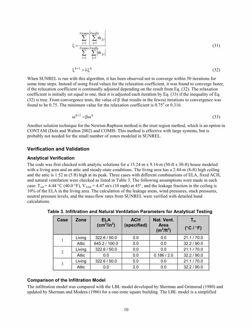
Comparison of the Infiltration Model The infiltration model was compared with the LBL model developed by Sherman and Grimsrud (1980) and updated by Sherman and Modera (1986) for a one-zone square building. The LBL model is a simplified

10

single-zone model based on crack flow equations. This model computes the flow rates from the wind and stack effects separately and then it combines them in quadrature. In addition, the wind pressures are averaged over all the walls so that wind direction is not important and there is no wind effect on the horizontal surfaces. The LBL model has been compared with experimental results to validate its performance, and has been shown to slightly over predict the infiltration values on a long-term basis (Sherman and Modera 1986). The dimensions of the building are 15 m x 15 m x 2.4 m (49.2 ft x 49.2 ft x 7.87 ft) with an ELA of 500 cm2 (77.5 in2) and 25% of the ELA is in the roof and 25% is in the floor. The interior temperature is Tin = 20 °C (68 °F) and the terrain and shielding classes are three.

An almost exact agreement is observed in Figure 3 for the infiltration rate from the stack effect alone. The slight difference is due to SUNREL’s use of the outside air density for infiltration and the inside air density for exfiltration, while the LBL model uses a fixed air density of 1.2 kg/m3.

Air

Cha

nges

per

Hou

r

0.2

0.18

0.16

0.14

0.12

0.1

0.08

0.06

0.04

0.02

0

LBL SUNRE

0 5 10 15 20 25 30 35 40

Outdoor Temperature (°C) Figure 3. Comparison of SUNREL with the LBL infiltration model for stack effect

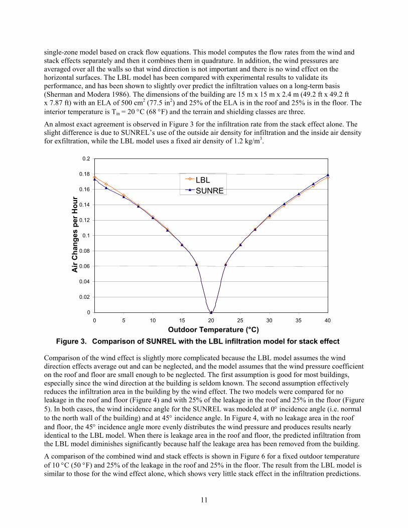
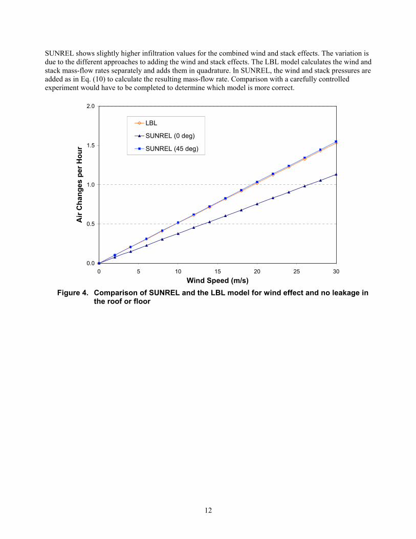
Comparison of the wind effect is slightly more complicated because the LBL model assumes the wind direction effects average out and can be neglected, and the model assumes that the wind pressure coefficient on the roof and floor are small enough to be neglected. The first assumption is good for most buildings, especially since the wind direction at the building is seldom known. The second assumption effectively reduces the infiltration area in the building by the wind effect. The two models were compared for no leakage in the roof and floor (Figure 4) and with 25% of the leakage in the roof and 25% in the floor (Figure 5). In both cases, the wind incidence angle for the SUNREL was modeled at 0° incidence angle (i.e. normal to the north wall of the building) and at 45° incidence angle. In Figure 4, with no leakage area in the roof and floor, the 45° incidence angle more evenly distributes the wind pressure and produces results nearly identical to the LBL model. When there is leakage area in the roof and floor, the predicted infiltration from the LBL model diminishes significantly because half the leakage area has been removed from the building.

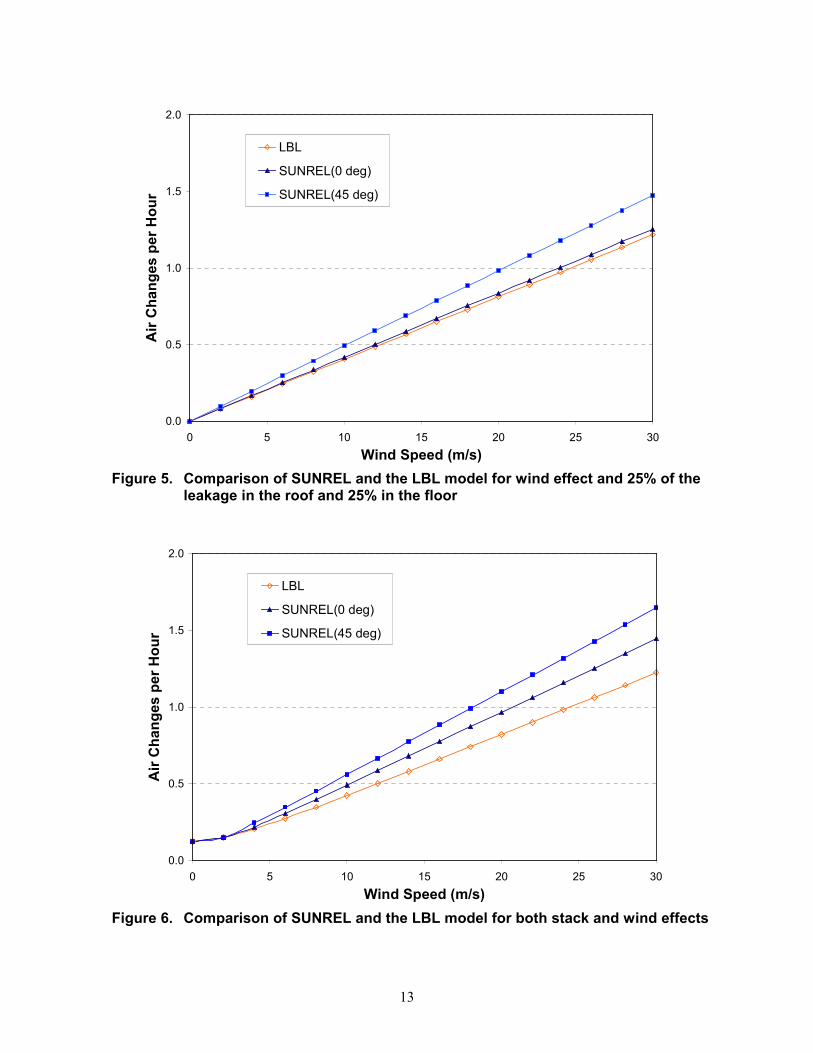
A comparison of the combined wind and stack effects is shown in Figure 6 for a fixed outdoor temperature of 10 °C (50 °F) and 25% of the leakage in the roof and 25% in the floor. The result from the LBL model is similar to those for the wind effect alone, which shows very little stack effect in the infiltration predictions.

11

SUNREL shows slightly higher infiltration values for the combined wind and stack effects. The variation is due to the different approaches to adding the wind and stack effects. The LBL model calculates the wind and stack mass-flow rates separately and adds them in quadrature. In SUNREL, the wind and stack pressures are added as in Eq. (10) to calculate the resulting mass-flow rate. Comparison with a carefully controlled experiment would have to be completed to determine which model is more correct.

2.0

1.5

1.0

0.5

0.0 0 5 10 15 20 25 30

LBL

SUNREL (0 deg)

SUNREL (45 deg)

Wind Speed (m/s) Figure 4. Comparison of SUNREL and the LBL model for wind effect and no leakage in

the roof or floor

Air

Cha

nges

per

Hou

r

12

2.0

1.5

1.0

0.5

0.0 0 5 10 15 20 25 30

LBL

SUNREL(0 deg)

SUNREL(45 deg)

Wind Speed (m/s) Figure 5. Comparison of SUNREL and the LBL model for wind effect and 25% of the

leakage in the roof and 25% in the floor

2.0

1.5

1.0

0.5

0.0 0 5 10 15 20 25 30

LBL

SUNREL(0 deg)

SUNREL(45 deg)

Wind Speed (m/s) Figure 6. Comparison of SUNREL and the LBL model for both stack and wind effects

Air

Cha

nges

per

Hou

r A

ir C

hang

es p

er H

our

13

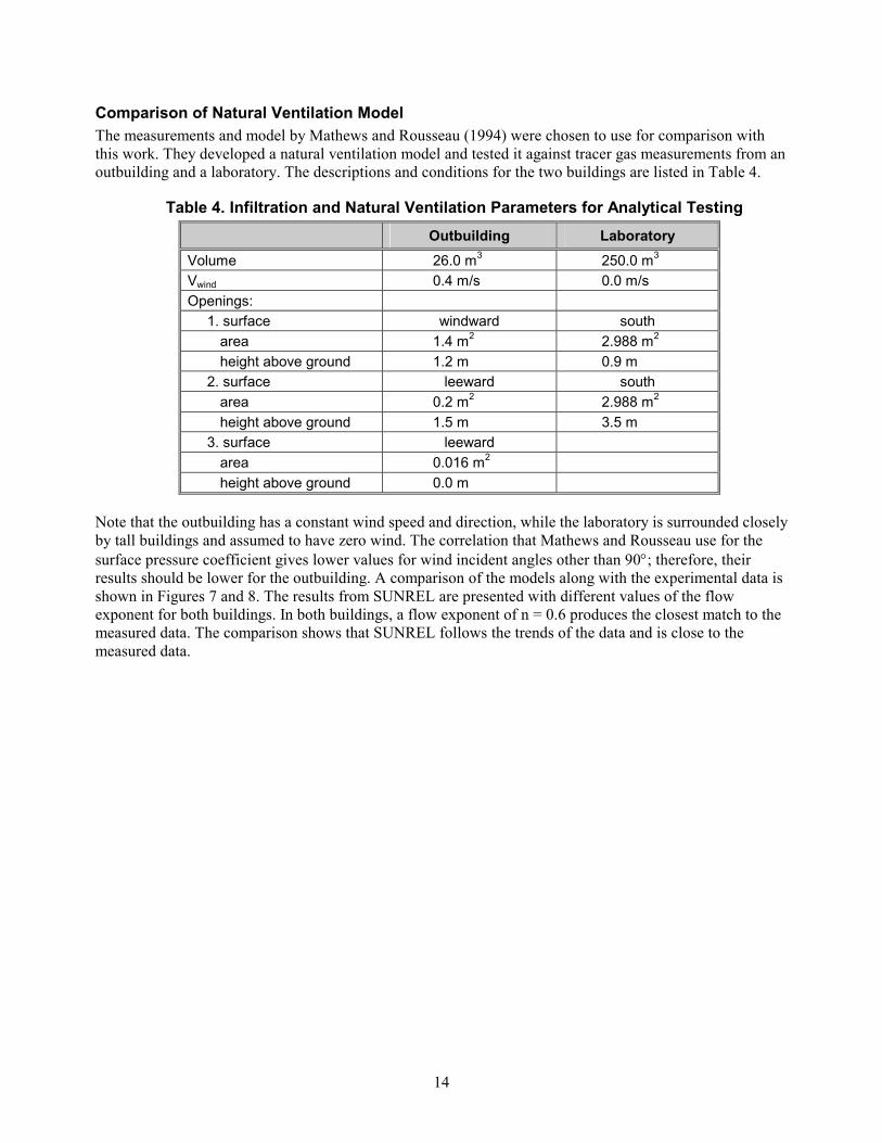
Comparison of Natural Ventilation Model The measurements and model by Mathews and Rousseau (1994) were chosen to use for comparison with this work. They developed a natural ventilation model and tested it against tracer gas measurements from an outbuilding and a laboratory. The descriptions and conditions for the two buildings are listed in Table 4.

Table 4. Infiltration and Natural Ventilation Parameters for Analytical Testing Outbuilding Laboratory

Volume 26.0 m3 250.0 m3

Vwind 0.4 m/s 0.0 m/s Openings:

1. surface windward south area m2 2.988 m2

height above ground 1.2 m 0.9 m 2. surface leeward south

area m2 2.988 m2

height above ground 1.5 m 3.5 m 3. surface leeward

area m2

height above ground 0.0 m

1.4

0.2

0.016

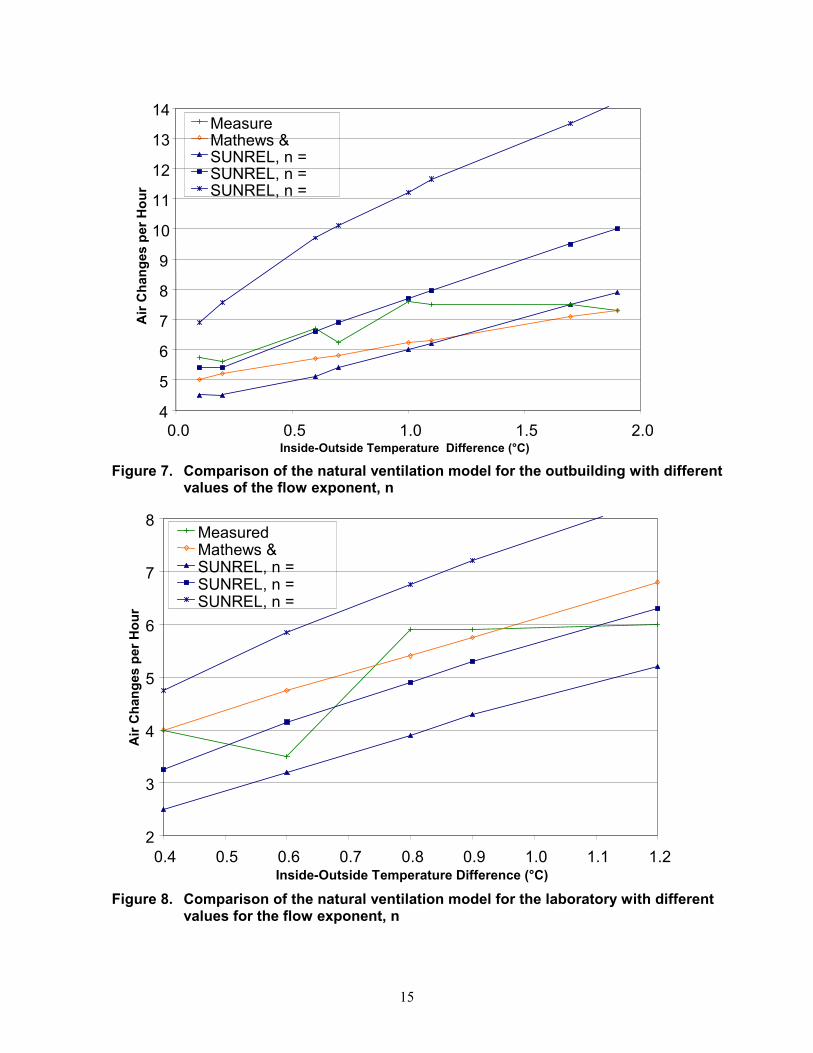
Note that the outbuilding has a constant wind speed and direction, while the laboratory is surrounded closely by tall buildings and assumed to have zero wind. The correlation that Mathews and Rousseau use for the surface pressure coefficient gives lower values for wind incident angles other than 90°; therefore, their results should be lower for the outbuilding. A comparison of the models along with the experimental data is shown in Figures 7 and 8. The results from SUNREL are presented with different values of the flow exponent for both buildings. In both buildings, a flow exponent of n = 0.6 produces the closest match to the measured data. The comparison shows that SUNREL follows the trends of the data and is close to the measured data.

14

14

13

12

11

10

9

8

7

6

5

4 0.0 0.5 1.0 1.5 2.0

Measure Mathews & SUNREL, n = SUNREL, n = SUNREL, n =

Inside-Outside Temperature Difference (°C)

Figure 7. Comparison of the natural ventilation model for the outbuilding with different values of the flow exponent, n

8

7

6

5

4

3

2 0.4 0.5 0.6 0.7 0.8 0.9 1.0 1.1 1.2

Measured Mathews & SUNREL, n = SUNREL, n = SUNREL, n =

Inside-Outside Temperature Difference (°C)

Figure 8. Comparison of the natural ventilation model for the laboratory with different values for the flow exponent, n

Air

Cha

nges

per

Hou

r A

ir C

hang

es p

er H

our

15

Summary A multizone infiltration model has been presented that incorporates measurements of a building’s leakage from blower door tests and measured weather data. The algorithms developed exhibit an effective compromise between the physical model, the accuracy of the known information, and the burden of required input. The average surface pressure from the wind on every surface, vertical as well as sloped, is modeled using a correlation based on wind tunnel measurements. The building terrain and local shielding are also taken into account. The model was verified with analytical calculations and against other proven models and physical measurements. Although, there are many unknowns, such as the crack distribution and wind profiles around the building, it is a great improvement over the simple models in SERI-RES.

The infiltration model was combined with the SUNREL whole-building energy simulation program to provide a simple infiltration and natural ventilation model for residential and small commercial buildings. The infiltration mass balance iteration loop is placed inside the zone energy balance iteration loop. This approach slightly increases the runtime, which varies with the number of zones and the amount of mass modeled in the building. If there is no thermal mass in the building model, the higher variations in zone temperature increase the number of iterations for the infiltration model and can introduce instabilities. The program has been extensively tested for robustness. The new program is included in a residential energy-auditing tool developed for a state energy agency.

There are areas of the model that could be enhanced or corrected. The current model does not include the effects of fans on zone pressures or model airflow through ducts, which are items not modeled in SUNREL. The model for flow through large external openings is very simple and limited to simple cases. In addition, the model does not include algorithms for airflow through large internal openings. This was not included due to the added complexity of the model and most residential buildings can be adequately modeled with one zone or multiple zones connected by a wall with no large openings. If a large opening model were included, the temperature stratification should also be modeled to correctly determine the flow through the openings.

References Aikens, R.E., 1976, Wind Pressures on Buildings, Phd Dissertation, Colorado State University, Fort Collins,

CO.

ASHRAE Handbook of Fundamentals, 2001, American Society of Heating, Refrigeration and Air-Conditioning Engineers, Atlanta, GA.

ASTM 1992, “Standard Test Method for Determining Air Leakage Rate by Fan Pressurization,” E779, American Society for Testing and Materials, Philadelphia, PA.

Deru, M., Judkoff, R., and Torcellini, P., 2002, SUNREL, Technical Reference Manual, NREL/BK-550-30193, National Renewable Energy Laboratory, Golden, CO.

Dols, W. S., 2001. “A Tool for Modeling Airflow & Contaminant Transport,” ASHRAE Journal, Vol. 43, No.3, pp. 35-42.

Dols, W. S. and Walton, G. N., 2002. CONTAMW 2.0 User Manual, NISTIR 6921, National Institute of Standards and Technology, U.S. Department of Commerce, Gaithersburg, MD.

Feustel, H.E. and Rayner-Hooson, A., 1990, COMIS Fundamentals, LBL-28560, Applied Science Division, Lawrence Berkeley National Laboratory, Berkeley, CA.

Feustel, H.E. and Dieris, J., 1992, “A survey of airflow models for multizone structures,” Energy and Buildings, Vol. 18, pp. 79-100.

Feustel, H.E. 1999, “COMIS – an international multizone airflow and contaminant transport model,” Energy and Buildings, Vol. 30, pp. 3-18.

16

Haghighat, F., Brohus, H., and Rao, J., 2000, “Modeling air infiltration due to wind fluctuations – a review,” Building and Environment, Vol. 35, pp. 377-385.

Hensen, J. 1995, “Modeling Coupled Heat and Airflow: Ping-Pong vs. Onions,” Proceedings, 16th AIVC Conference, Palm Springs, California.

Huang, J, Winkelmann, F., Buhl, F., Pedersen, C., Fisher, D., Liessen, R., Taylor, R., Strand, R., Crawley, D., and Lawrie, L. 1999. “Linking the COMIS Multizone Airflow Model with the EnergyPlus Building Energy Simulation Program,” Proc. Building Simulation 99, Kyoto, Japan, September.

Kendrick, J. 1993. An Overview of Combined Modeling of Heat Transport and Air Movement, International Energy Agency, Technical Note AIVC 40, The Air Infiltration and Ventilation Centre, University of Warwick Science Park, Conventry, UK.

Kreyszig, E., 1988, Advanced Engineering Mathematics, sixth edition, John Wiley & Sons, New York.

Li, Y., Delsante, A., and Symons, J., 2000. “Prediction of natural ventilation in buildings with large openings,” Building and Environment, Vol. 35, pp. 191-206.

Liddament, M.W., 1988, “The Calculation of Wind Effect on Ventilation,” Symposium on Wind Effects on Ventilation, AHSRAE Transactions, Vol. 94(2), pp. 1645-1659.

Mathews, E.H. and Rousseau, P.G., 1994, “A New Integrated Design Tool for Naturally Ventilated Buildings Part 1: Ventilation Model,” Building and Environment, n. 29, pp. 461-72.

Riffat, S.B., 1991, “Algorithms for Airflows Through Large Internal and External Openings,” Applied Energy, Vol. 40, pp. 171-88.

SERI-RES Users Manual, version 1.0, 1988 Solar Energy Research Institute, Golden, CO.

Sherman, M.H. and Grimsrud, D.T., 1980, “Infiltration-Pressurization Correlation: Simplified Physical Modeling,” ASHRAE Transactions, Vol. 86(2), pp. 778-803.

Sherman, M.H. and Modera, M.P., 1986, “Comparison of Measured and Predicted Infiltration Using the LBL Infiltration Model,” Proceedings Measured Air Leakage of Buildings, ASTM STP 904 ASTMS, Philadelphia, ASTM, pp. 325-347.

Stathopoulos, T., Dhiovitti, D. and Dodaro, L., 1994, “Wind Shielding Effects of Trees on Low Buildings,” Building and Environment, Vol. 29, No. 2, pp. 141-150.

Swami, M.V. and Chandra S., 1988, “Correlations for Pressure Distribution of Buildings and Calculation of Natural-Ventilation Airflow,” ASHRAE Transactions, Vol. 94(1), pp. 243-66.

Walton, G.N., 1982, “Airflow and Multiroom Thermal Analysis,” ASHRAE Transactions, Vol. 88(2), pp. 78-91.

Walton, G.N., 1989, AIRNET - A Computer Program for Building Airflow Network Modeling, NISTIR 89-4072, National Institute of Standards and Technology, U.S. Department of Commerce, Gaithersburg, MD.

17

REPORT DOCUMENTATION PAGE Form Approved OMB NO. 0704-0188

Public reporting burden for this collection of information is estimated to average 1 hour per response, including the time for reviewing instructions, searching existing data sources,gathering and maintaining the data needed, and completing and reviewing the collection of information. Send comments regarding this burden estimate or any other aspect of this collection of information, including suggestions for reducing this burden, to Washington Headquarters Services, Directorate for Information Operations and Reports, 1215 JeffersonDavis Highway, Suite 1204, Arlington, VA 22202-4302, and to the Office of Management and Budget, Paperwork Reduction Project (0704-0188), Washington, DC 20503.

1. AGENCY USE ONLY (Leave blank) 2. REPORT DATE March 2003

3. REPORT TYPE AND DATES COVERED Conference Paper

4. TITLE AND SUBTITLE Infiltration and Natural Ventilation Model for Whole-Building Energy Simulation of Residential Buildings: Preprint

6. AUTHOR(S) M. Deru and P. Burns

5. FUNDING NUMBERS

BEC3.4005

7. PERFORMING ORGANIZATION NAME(S) AND ADDRESS(ES) National Renewable Energy Laboratory 1617 Cole Blvd. Golden, CO 80401-3393

8. PERFORMING ORGANIZATION REPORT NUMBER

NREL/CP-550-33698

9. SPONSORING/MONITORING AGENCY NAME(S) AND ADDRESS(ES) 10. SPONSORING/MONITORING AGENCY REPORT NUMBER

11. SUPPLEMENTARY NOTES

12a. ISTRIBUTION/AVAILABILITY STATEMENT National Technical Information Service U.S. Department of Commerce 5285 Port Royal Road Springfield, VA 22161

12b. ISTRIBUTION CODE

13. ABSTRACT (Maximum 200 words)

The infiltration term in the building energy balance equation is one of the least understood and most difficult to model. For many residential buildings, which have an energy performance dominated by the envelope, it can be one of the most important terms. There are numerous airflow models; however, these are not combined with whole-building energy simulation programs that are in common use in North America. s paper describes a simple multizone nodal airflow model integrated with the SUNREL whole-building energy simulation program.

15. NUMBER OF PAGES 14. SUBJECT TERMS

SUNREL; residential; airflow; energy simulation; infiltration; natural ventilation 16. PRICE CODE

17. SECURITY CLASSIFICATION OF REPORT Unclassified

18. SECURITY CLASSIFICATION OF THIS PAGE Unclassified

19. SECURITY CLASSIFICATION OF ABSTRACT Unclassified

20. LIMITATION OF ABSTRACT

UL

D D

Thi

NSN 7540-01-280-5500 Standard Form 298 (Rev. 2-89) Prescribed by ANSI Std. Z39-18

298-102