inference for diffusion processes and stochastic ... · inference for diffusion processes and ......
TRANSCRIPT
Inference for
Diffusion Processes and
Stochastic Volatility Models
Ph.D. thesis
Helle Sørensen
University of CopenhagenSeptember 2000

Inference for Diffusion Processes
and Stochastic Volatility ModelsPh.D. thesis
Helle SørensenDepartment of Statistics and Operations ResearchInstitute for Mathematical SciencesFaculty of ScienceUniversity of Copenhagen
Thesis advisor: Martin Jacobsen, University of CopenhagenThesis committee: Michael Sørensen, University of Copenhagen
Uwe Küchler, Humboldt University of BerlinBo Martin Bibby, KVL, Copenhagen

Helle SørensenDepartment of Statistics and Operations ResearchUniversity of CopenhagenUniversitetsparken 5DK-2100 Copenhagen EastDenmarkhsoerenmath.ku.dkhttp://www.math.ku.dk/~hsoeren
Preface
This thesis has been prepared in partial fulfillment of the requirements for thePh.D. degree at the Department of Statistics and Operations Research, Institutefor Mathematical Sciences at the University of Copenhagen. The work has beencarried out in the period from May 1997 to July 2000 with Martin Jacobsen asthesis advisor.
The thesis contains a brief overall introduction, two introductory chapters andthree papers. The introductory chapters have been prepared for this thesis exclu-sively whereas the papers have been (or will shortly be) submitted for publication.Each chapter and paper is self-contained and can be read independently from therest. The first page of each of the three papers contain an abstract and detailson publication. Page numbers within the papers are given in parentheses at thebottom of each page, underlining that the papers have been prepared and writtenseparately. To emphasize the unity of the thesis, pages are also numbered consec-utively (at the top of each page) and the lists of references are collected in one
bibliography placed at the end of the thesis.The present version differs from the original one which was submitted for the
Ph.D. degree on July 20, 2000, by this preface and in that a minor number of typosand misprints have been corrected.
Acknowledgements
I would like to thank my supervisor Martin Jacobsen for his encouragement and fornumerous valuable suggestions and discussions during the last three years. Thanksare also due to Martin for careful reading of earlier versions of the chapters andpapers. Also, I would like to thank Søren Feodor Nielsen for his ideas and helpon empirical processes. Thanks are also due to everyone at the department formaking everyday life enjoyable.
Part of the work was done while I was visiting Department of Statistics atUniversity of California, Berkeley. I thank everyone there for making it such apleasant stay.
Jens Lund, Bo Markussen, Søren Feodor Nielsen, Henning Niss and MartinRichter have all read various parts of the manuscript. I am grateful for their com-ments and constructive critics.
Copenhagen, September 2000
Helle Sørensen

Summary
Diffusion processes have a wide range of applications. In physics and biologythey are used for modeling phenomena assumed to evolve randomly and contin-uously in time. In mathematical finance they are used for modeling various priceprocesses. Data are essentially always sampled at discrete points in time only.This leaves the statistician in a dilemma because the few models that are easy tohandle statistically, in general do not describe data adequately. For example, itis well known that stock price data usually violate the assumptions of the geo-metric Brownian motion (or in finance terms, the Black-Scholes model) classicallyused for stock price modeling. For more complicated models maximum likelihoodestimation is usually not possible because the discrete-time transitions implicitlydefined by the continuous-time model are not known analytically. Consequently,there is a need for alternative statistical methods.
The first part of this thesis (Chapter 2 and Papers I and II) is about para-
metric inference for stationary and ergodic diffusion processes with general, oftennon-linear, specifications of the drift and diffusion functions. Chapter 2 providesan overview of existing techniques with emphasis on estimating functions. Fur-thermore, new results on identification for martingale estimating functions arepresented. In Paper I a simple, explicit approximation of the continuous-timescore function is derived in terms of the infinitesimal generator and the invariantdensity. As opposed to the usual Riemann-Itô approximation, it is unbiased andprovides consistent estimators. Paper II presents a method suitable for estima-tion of parameters in the diffusion term. It is based on a functional relationshipbetween the drift, the diffusion function and the invariant density, and providessatisfactory estimates in the difficult CKLS model. The usual limit theory does notapply; instead empirical process theory is employed in order to prove asymptoticproperties of the estimator.
The second part of the thesis (Chapter 3 and Paper III) is about parametric
inference for stochastic volatility models, that is, two-dimensional diffusion modelswith a special structure and one of the coordinates unobservable. The introduc-tion of a latent process makes it possible to retain a simple (linear) structure of themodel and still create the complex data structures known from empirical studies.However, it also complicates the statistical analysis because the model is only par-tially observed. Chapter 3 provides an introduction to stochastic volatility modelswith special emphasis on four particular models and on statistical analysis. A com-parison of different models shows that the increments of the observable processcan have almost identical distributions although the underlying latent processes
vi Summary
are specified quite differently. Still, the models differ in their ability to createhighly leptokurtic distributions. The overview of estimation methods covers awide range of techniques from simple moment-based methods to quite compli-cated techniques relying on very intensive computations. In Paper III a new ap-proximate maximum likelihood method is presented. The idea is to pretend thatthe increments of the observable process form a k’th order Markov chain for somerelatively small k. The corresponding approximate score function is unbiased, andthe estimators therefore consistent, for each fixed k because the true conditionaldistributions given the k previous observations are used. These conditional densi-ties are not known analytically but can be computed by simulation. The methodmakes it thereby possible to compute quite natural approximations to the likeli-hood function.
Dansk resumé
Diffusionsprocesser har anvendelsesmuligheder indenfor adskillige fagområder.De benyttes til beskrivelse af fænomener der varierer kontinuert og stokastisk overtid, for eksempel i fysik og biologi. De benyttes også intensivt i matematisk finan-siering til beskrivelse af prisfluktuationer på forskellige finansielle aktiver. Uan-set antagelsen om kontinuert variation er observationer af processerne dog altiddiskrete af natur idet målinger foretages på endeligt mange, adskilte tidspunk-ter. Dette komplicerer den statistiske analyse betydeligt fordi overgangssandsyn-lighederne, implicit defineret af modellen, kun er kendt analytisk for ganske fåmodeller. Disse modeller er som regel for simple til at beskrive strukturen i deobserverede data tilfredsstillende. For eksempel er det velkendt at faktisk obser-verede aktiekurser er i klar modstrid med den geometriske brownske bevægelse(eller med terminologi fra finansiering: Black-Scholes modellen) som ellers klas-sisk set er blevet brugt som model for aktiekurser. Det er med andre ord sjældentmuligt udføre maksimaliseringsestimation, og der er således behov for alternativeestimationsmetoder.
Afhandlingens første del (kapitel 2 og artikel I og II) handler om parametrisk
inferens for generelle stationære og ergodiske diffusionsprocesser. Kapitel 2 giver enoversigt over eksisterende estimationsmetoder med hovedvægt på teorien for esti-mationsfunktioner. Udover en redegørelse for velkendte metoder og resultaterpræsenteres også et nyt resultat om identifikation for martingalestimationsfunk-tioner. I artikel I udledes en simpel, eksplicit approksimation af scorefunktionenhørende til en observation i kontinuert tid. Approksimationen er en central esti-mationfunktion og giver derfor, til forskel fra den sædvanlige Riemann-Itô approk-simation, konsistente estimatorer. I artikel II beskrives en metode til estimation afparametre i diffusionsfunktionen. Metoden er baseret på en punktvis sammen-hæng mellem driftfunktionen, diffusionsfunktionen og tætheden for den statio-nære begyndelsesfordeling, og den giver fornuftige estimater i den ellers vanske-lige CKLS model. De klassiske grænsesætniger kan ikke anvendes; i stedet benyttesteorien om empiriske processer til at bevise asymptotiske egenskaber for estima-torerne.
Afhandlingens anden del (kapitel 3 og artikel III) handler om parametrisk infe-
rens for stokastiske volatilitetsmodeller, dvs. todimensionale diffusionsmodeller derhar en speciel form og hvor kun den ene af koordinaterne er observerbar. Ind-førelsen af den ekstra proces gør det muligt at frembringe fænomenerne kendtfra empiriske analyser ved hjælp af relativt simple (lineære) modeller, men denstatistiske analyse kompliceres fordi modellen kun observeres partielt. Kapitel 3
viii Dansk resumé
er en introduktion til stokastiske volatilitetsmodeller med særligt henblik på firespecifikke modeller og på statistisk analyse. En sammenligning viser at forskelligemodeller for den ikke-observerbare process kan frembringe næsten identiske for-delinger for tilvæksterne af den observerbare process, men at modellerne adskillersig fra hinanden ved deres evne til at skabe tilvækster med meget tunge haler.Oversigten over estimationsmetoder for stokastiske volatilitetsmodeller spænderfra enkle momentbaserede metoder til ganske komplicerede og meget beregnings-krævende metoder. I artikel III præsenteres en ny approksimativ maximumlike-lihoodmetode. Ideen er at opføre sig som om tilvæksterne for den observerbareprocess udgør en markovkæde af orden k for et relativt lille k. Centraliteten af dentilsvarende scorefunktion bibeholdes såfremt de sande betingede tætheder givetde k foregående observationer benyttes. Således bliver estimatoren konsistent ogasymptotisk normalfordelt for ethvert fast k. De betingede tætheder er ikke kendtanalytisk men kan beregnes ved simulation. Metoden gør det dermed muligt atberegne naturlige approksimationer til likelihoodfunktionen.
Table of Contents
Preface iii
Summary v
Dansk resumé vii
Table of Contents ix
1 Introduction 1
2 Inference for diffusion processes 5
2.1 Model, assumptions and notation . . . . . . . . . . . . . . . . . . . 62.2 Preliminary comments on estimation . . . . . . . . . . . . . . . . . 72.3 Estimating functions . . . . . . . . . . . . . . . . . . . . . . . . . . 82.4 Approximate maximum likelihood estimation . . . . . . . . . . . . 162.5 Bayesian analysis . . . . . . . . . . . . . . . . . . . . . . . . . . . . 192.6 Estimation based on auxiliary models . . . . . . . . . . . . . . . . . 212.7 Estimation of parameters in the diffusion term . . . . . . . . . . . . 222.8 Conclusion . . . . . . . . . . . . . . . . . . . . . . . . . . . . . . . 23
3 Stochastic volatility models 25
3.1 A modification of the Black-Scholes model . . . . . . . . . . . . . . 253.2 The class of models . . . . . . . . . . . . . . . . . . . . . . . . . . . 263.3 Four particular models . . . . . . . . . . . . . . . . . . . . . . . . . 283.4 Estimation methods . . . . . . . . . . . . . . . . . . . . . . . . . . 363.5 Related models . . . . . . . . . . . . . . . . . . . . . . . . . . . . . 503.6 Conclusion . . . . . . . . . . . . . . . . . . . . . . . . . . . . . . . 54
Papers
I Approximation of the Score Function 55
I.1 Introduction . . . . . . . . . . . . . . . . . . . . . . . . . . . . . . . 56I.2 Model and notation . . . . . . . . . . . . . . . . . . . . . . . . . . . 56I.3 The estimating function . . . . . . . . . . . . . . . . . . . . . . . . 57I.4 Asymptotic properties . . . . . . . . . . . . . . . . . . . . . . . . . 61I.5 Examples . . . . . . . . . . . . . . . . . . . . . . . . . . . . . . . . 61
x Table of Contents
I.6 Multi-dimensional processes . . . . . . . . . . . . . . . . . . . . . . 63
II Estimation of Diffusion Parametersfor Discretely ObservedDiffusion Processes 67
II.1 Introduction . . . . . . . . . . . . . . . . . . . . . . . . . . . . . . . 68II.2 Model and notation . . . . . . . . . . . . . . . . . . . . . . . . . . . 69II.3 Estimation . . . . . . . . . . . . . . . . . . . . . . . . . . . . . . . . 71II.4 Consistency . . . . . . . . . . . . . . . . . . . . . . . . . . . . . . . 77II.5 Further asymptotic results . . . . . . . . . . . . . . . . . . . . . . . 79II.6 When the drift is not known . . . . . . . . . . . . . . . . . . . . . . 86II.7 Examples . . . . . . . . . . . . . . . . . . . . . . . . . . . . . . . . 86II.8 Concluding remarks . . . . . . . . . . . . . . . . . . . . . . . . . . 98II.A Appendix: On empirical process theory . . . . . . . . . . . . . . . . 99II.B Appendix: A mixing result for the OU-process . . . . . . . . . . . . 109
III Simulated Likelihood Approximationsfor Stochastic Volatility Models 113
III.1 Introduction . . . . . . . . . . . . . . . . . . . . . . . . . . . . . . . 114III.2 Model and basic assumptions . . . . . . . . . . . . . . . . . . . . . 116III.3 Approximations to the likelihood function . . . . . . . . . . . . . . 121III.4 Computational aspects . . . . . . . . . . . . . . . . . . . . . . . . . 125III.5 Asymptotic results . . . . . . . . . . . . . . . . . . . . . . . . . . . 127III.6 Efficiency considerations . . . . . . . . . . . . . . . . . . . . . . . . 134III.7 Example: The Cox-Ingersoll-Ross process . . . . . . . . . . . . . . . 136III.8 Conclusion . . . . . . . . . . . . . . . . . . . . . . . . . . . . . . . 151III.A Appendix: Miscellaneous . . . . . . . . . . . . . . . . . . . . . . . . 152III.B Appendix: Results from the simulation study . . . . . . . . . . . . . 155
Bibliography 159
1Introduction
Diffusion models have a large range of applications. They have been used for along time to model phenomena evolving randomly and continuously in time, e.g.
in physics and biology. During the last thirty years or so the models have also beenapplied intensively in mathematical finance for describing stock prices, exchangerates, interest rates, etc. (although it is well-known that such quantities do notreally change continuously in time).
Data are essentially always recorded at discrete points in time only (e.g. weekly,daily or each minute) and can thus be interpreted as time series data. Still,continuous-time models are often preferred to classical time series models. Thereare (at least) two reasons for this. First, if data are sampled at irregularly spacedtime-points, then an appropriate discrete-time model should incorporate this ex-plicitly. As opposed to this, continuous-time models implicitly define transitionsover time intervals of any length in a consistent way. For example, missing datain a sample where time-points for observations are otherwise regularly spaced, donot give rise to serious problems in the continuous-time setting as they are treatedjust like the values not observed due to discrete-time sampling. Second, all themachinery from stochastic calculus is at our disposal when we use diffusion mod-els. This has proved important in finance theory where derivation of various priceformulas usually relies heavily on this theory.
Thus convinced that diffusion models are important and useful alternatives toclassical time series models I turn to the statistical analysis. I shall be concernedwith parametric inference exclusively. For a few models, estimation is straight-forward because the corresponding stochastic differential equation can be solvedexplicitly. This is the case for the geometric Brownian motion, the Ornstein-Uhlenbeck process and the square-root process which have log-normal, normaland non-central chi-square transition probabilities respectively. However, “nature”(or “the market”) most often generates data not adequately described by such sim-ple models. For example, empirical studies clearly reveal that increments of loga-rithmic stock prices are not independent and Gaussian as implied by the geometricBrownian motion classically used for stock price modeling. Rather, they exhibittemporal dependence and leptokurtosis. Consequently, more complex models areneeded in order to obtain reasonable agreement with data. This complicates thestatistical analysis considerably because the discrete-time transitions (implicitlydefined by the model) are no longer known analytically. Specifically, the likelihood
function is usually not tractable. In other words, one has to use models for whichlikelihood analysis is not possible, and there is consequently a need for alternative
2 Chapter 1. Introduction
methods.
In this thesis I am concerned with parametric inference for two types of gener-alizations of the above simple models, namely (one-dimensional) diffusion mod-els with more general, typically non-linear, specifications of drift and diffusionfunctions, and continuous-time stochastic volatility models. By the latter I meantwo-dimensional diffusion processes with a special structure and one of the coordi-nates unobservable. The introduction of an extra, latent process makes it possibleto retain a simple (linear) structure of the stochastic differential equation for theobservable process and still create the characteristic features known from empir-ical studies. However, the extra process also complicates the statistical analysisbecause the model is only partially observed.
Further introductory comments on the two model types and the correspondingestimation problems are given in the beginning of Chapters 2 and 3.
Structure of the thesis
My main contributions in this thesis are contained in three papers: Papers I and IIon (pure) diffusion models and Paper III on stochastic volatility models. In addi-tion I provide two introductory chapters: Chapter 2 on diffusions and Chapter 3 onstochastic volatility models. The aim of the two introductory chapters is mainly toprovide overviews of existing estimation methods, but they also contain a few newresults. I do not know of any review papers with quite the same focus. The chap-ters and papers may be read independently. This has the unfortunate consequencethat models, notation, etc. are defined several times. Attempts have been madein order to customize notation; still, there may be slight differences which shouldcause no confusion. The lists of references have been collected to one bibliographyplaced at the end of the thesis.
Estimation in (pure) diffusion models. Chapter 2 provides an overview of ex-isting estimation techniques for stationary and ergodic diffusion processes. Mainemphasis is on estimating functions, in particular on martingale estimating func-tions and so-called simple estimating functions. Well-known properties and resultsare reviewed, and some some new results concerning identification for martingaleestimating functions are presented: one of the regularity conditions needed in or-der for the estimator to be asymptotically well-behaved is explained in terms ofreparametrizations. In addition to estimating functions, the chapter covers threeapproximate maximum likelihood methods, Bayesian analysis and methods basedon auxiliary models.
Papers I and II contain my main contributions in the area of estimation indiffusion models. Brief reviews are given in Sections 2.3.2 and 2.7. In Paper I(Discretely Observed Diffusions: Approximation of the Continuous-time Score Func-
tion) I study how the structure of the continuous-time score function can be usedwhen only discrete-time observations are available. The usual Riemann-Itô ap-proximation is biased; I derive an alternative, unbiased approximation in terms of
Structure of the thesis 3
the infinitesimal generator and the invariant density. The approximation is an ex-plicit, so-called simple estimating function; is is invariant to data transformations;and it provides consistent and asymptotically normal estimators as the number ofobservations increases (for any fixed time interval between observations). The ap-proach carries over to multi-dimensional diffusions (to some extent at least), andI study a few examples where the method works very well.
In Paper II (Estimation of Diffusion Parameters for Discretely Observed Diffusion
Processes) I discuss a method suitable for estimation of parameters in the diffusionterm when the drift is known. It is based on a functional relationship betweenthe drift, the diffusion function and the invariant density. I apply the methodto simulated data from the relatively difficult CKLS model and get satisfactoryestimates. The estimators are probably not efficient, though. From a theoreticalpoint of view the derivation of asymptotic results is perhaps most interesting. Theusual limit theory does not apply; instead I employ empirical process theory. I amnot aware of other applications of empirical process theory to problems related todiscretely observed diffusions.
Stochastic volatility models. Chapter 3 is an introduction to stochastic volatil-ity models in continuous time. I study four particular models in detail and con-clude that they mainly differ in their ability to create processes for which the incre-ments are highly leptokurtic. If parameter values are chosen appropriately, thenthe models are hard to distinguish. I do not know of any similar comparisons inthe literature. Chapter 3 also provides an overview of existing estimation methods,some of which are developed very recently. The overview covers moment meth-ods, approximations to the marginal distribution of the increments, prediction-based estimating functions, Bayesian analysis, indirect inference and EMM, and afiltering-based method. Strikingly, most methods are extremely computationallyintensive.
My main contribution consists of a new approximate maximum likelihoodmethod, developed in Paper III (Simulated Likelihood Approximations for Stochas-
tic Volatility Models) and reviewed in Section 3.4.7. The method provides a se-quence of approximations to the likelihood function. For the k’th approximation,the idea is to pretend that the increments of the observable process form a k’thorder Markov chain. The corresponding approximate score function is unbiasedbecause the true conditional distributions given the k previous observations areused. For any fixed k the estimator is invariant to transformations of data, consis-tent and asymptotically normal (for any fixed time interval between observations).There is no closed-form expression for the approximate likelihood function (justas for the true likelihood function) but it can be computed by simulation. I ap-ply the method to simulated data in Paper III and to Microsoft stock price data inSection 3.4.7.
Finally, let me stress that although diffusion-type models are perhaps mostwidely applied in finance these days, and although the applications mentioned

4 Chapter 1. Introduction
originate from finance, the focus of this thesis is purely statistical! My main in-terest in the models lies in their statistical properties rather than their financialapplications.
2Inference for diffusion processes
Statistical inference for diffusion processes has been an active research area duringthe last two or three decades. The work has developed from estimation of linearsystems from continuous-time observations (see Le Breton (1974) and the refer-ences therein) to estimation of non-linear systems (parametric or non-parametric)from discrete-time observations. In this chapter, as well as in Papers I and II, weshall be concerned with parametric inference for discrete-time observations exclu-sively. The models may be linear or non-linear.
This branch of research commenced in the mid eighties (with the paper byDacunha-Castelle & Florens-Zmirou (1986) on the loss of information due to dis-cretization as an important reference) and accelerated in the nineties. Importantreferences from the mid of the decade are Bibby & Sørensen (1995) on martingaleestimating functions, Gourieroux, Monfort & Renault (1993) on indirect inference,and Pedersen (1995b) on approximate maximum likelihood methods, among oth-ers. Later work includes Bayesian analysis (Elerian, Chib & Shephard 2000) andfurther approximate likelihood methods (Aït-Sahalia 1998, Poulsen 1999).
Ideally, the parameter should be estimated by maximum likelihood but, ex-cept for a few models, the likelihood function is not available analytically. In thischapter we review some of the alternatives proposed in the literature. There ex-ist review papers on estimation via estimating functions (Bibby & Sørensen 1996,Sørensen 1997), but we do not know of any surveys covering all the techniquesdiscussed in this chapter.
Papers I and II contain my main contributions in this area. Furthermore, thereare some new results on identification for martingale estimating functions in Sec-tion 2.3.1. In Paper I we discuss a particular estimating function derived as anapproximation to the continuous-time score function. The estimating function isof the so-called simple type, it is unbiased and invariant to data transformationsand provides consistent and asymptotically normal estimators. In Paper II we dis-cuss a method suitable for estimation of parameters in the diffusion term when thedrift is known. It is based on a functional relationship between the drift, the diffu-sion function and the invariant density, and provides asymptotically well-behavedestimators. The asymptotic results are proved using empirical process theory.
In the following we focus on fundamental ideas and refer to the literature forrigorous treatments. In particular, we consider one-dimensional diffusions only,although most methods apply in the multi-dimensional case as well. Also, we donot account for technical assumptions, regularity conditions etc. An exception is
6 Chapter 2. Inference for diffusion processes
Section 2.3.1, though, where the new identification results are presented.The chapter is organized as follows. The model is defined in Section 2.1,
and Section 2.2 contains preliminary comments on the estimation problem. Sec-tion 2.3 is about estimating functions with special emphasis on martingale estimat-ing functions and so-called simple estimating functions, including the one fromPaper I. In Sections 2.4 we discuss three approximations of the likelihood whichcan in principle be made arbitrarily accurate, and Section 2.5 is about Bayesiananalysis. In Section 2.6 we discuss indirect inference and EMM which both intro-duce auxiliary (but wrong) models and correct for the implied bias by simulation.The method from Paper II is reviewed in Section 2.7 and conclusions are finallydrawn in Section 2.8.
2.1 Model, assumptions and notation
In this section we present the model and the basic assumptions, and introducenotation that will be used throughout the chapter. We consider a one-dimensional,time-homogeneous stochastic differential equation
dXt = b(Xt;θ)dt +σ(Xt ;θ)dWt (2.1)
defined on a filtered probability space (Ω;F ;Ft;Pr). Here, W is a one-dimensionalBrownian motion and θ is an unknown p-dimensional parameter from the pa-rameter space Θ Rp . The true parameter value is denoted θ0. The functionsb :RΘ!R and σ :RΘ! (0;∞) are known and assumed to be suitably smooth.
The state space is denoted I = (l;r) for ∞ l < r +∞ (implicitly assumingthat it is open and the same for all θ). We shall assume that for any θ 2Θ and anyF0-measurable initial condition U with state space I, equation (2.1) has a uniquestrong solution X with X0 = U . Assume furthermore that there exists an invariant
distribution µθ = µ(x;θ)dx such that the solution to (2.1) with X0 µθ is strictlystationary and ergodic. It is well-known that sufficient conditions for this can beexpressed in terms of the scale function and the speed measure (see Section II.2,or the textbook by Karatzas & Shreve (1991)), and that µ(x;θ) is given by
µ(x;θ) = M(θ)σ2(x;θ)s(x;θ)1(2.2)
where logs(x;θ) = 2R x
x0b(y;θ)=σ2(y;θ)dy for some x0 2 I and M(θ) is a normal-
izing constant.For all θ 2 Θ the distribution of X with X0 µθ is denoted by Pθ . Under Pθ all
Xt µθ . Further, let for t 0 and x 2 I, pθ (t;x; ) denote the conditional density(transition density) of Xt given X0 = x. Since X is time-homogeneous pθ (t;x; ) isactually the density of Xs+t conditional on Xs = x for all s 0. Note that the tran-sition probabilities are most often analytically intractable whereas the invariantdensity is easy to find (at least up the normalizing constant).
We are going to need some matrix notation: Vectors in Rp are considered asp 1 matrices and AT is the transpose of A. For a function f = ( f1; : : : ; fq)T :
2.2. Preliminary comments on estimation 7RΘ ! Rq we let f 0(x;θ) and f 00 denote the matrices of first and second orderpartial derivatives with respect to x, and f (x;θ) = ∂θ f (x;θ) denote the q p ma-trix of partial derivatives with respect to θ , i.e. f jk = ∂ f j=∂θk, assuming that the
derivatives exist.Finally, introduce the differential operator Aθ given byAθ f (x;θ) = b(x;θ) f 0(x;θ)+ 1
2σ2(x;θ) f 00(x;θ) (2.3)
for twice continuously differentiable functions f : RΘ ! R. When restricted toa suitable subspace, Aθ is the infinitesimal generator of X (see Rogers & Williams(1987), for example).
2.2 Preliminary comments on estimation
The objective of this chapter is estimation of the parameter θ . First note thatif X is observed continuously from time zero to time T then parameters from thediffusion coefficient can be determined (rather than estimated) from the quadraticvariation process of X , and the remaining part can be estimated by maximumlikelihood: if the diffusion function is completely known, that is σ(x;θ) = σ(x),then the likelihood function for X0tT is given by
LcT (θ) = exp
Z T
0
b(Xs;θ)σ2(Xs) dXs 1
2
Z T
0
b2(Xs;θ)σ2(Xs) ds
: (2.4)
An informal argument for this formula is given below; for a proper proof seeLipster & Shiryayev (1977, Chapter 7).
From now on we shall consider the situation where X is observed at discretetime-points only. For convenience we consider equidistant time-points ∆;2∆; : : : ;n∆for some ∆ > 0. Conditional on the initial value X0, the likelihood function is givenas the product
Ln(θ) = n
∏i=1
pθ (∆;X(i1)∆;Xi∆)because X is Markov. Ideally, θ should be estimated by the value maximizingLn(θ), but since the transition probabilities are not analytically known, neither isthe likelihood function.
There are a couple of obvious, very simple alternatives which unfortunately arenot satisfactory. First, one could ignore the dependence structure and simply ap-proximate the conditional densities by the marginal density. Then all informationdue to the time evolution of X is lost, and it is usually not possible to estimate thefull parameter vector. See Section 2.3.2 for further details.
As a second alternative, one could use the Euler scheme (or some higher-orderscheme) given by the approximation
Xi∆ X(i1)∆ +b(X(i1)∆;θ)∆+σ(X(i1)∆;θ)p∆εi
8 Chapter 2. Inference for diffusion processes
where εi, i = 1; : : : ;n are independent, identically N(0;1)-distributed. This approxi-mation is good for small values of ∆ but may be bad for larger values. The approx-imation is two-fold: the moments are not the true conditional moments, and thetrue conditional distribution need not be Gaussian. The moment approximationintroduces bias implying that the corresponding estimator is inconsistent as n!∞for any fixed ∆ (Florens-Zmirou 1989). The Gaussian approximation introducesno bias per se, but usually implies inefficiency: if the conditional mean and vari-ance are replaced by the true ones, but the Gaussian approximation is maintained,then the corresponding approximation to the score function is a non-optimal mar-tingale estimating function, see Section 2.3.1.
Note that the Euler approximation provides an informal explanation of formula(2.4): if σ does not depend on θ , then the Euler approximation to the discrete-time likelihood function is given by (except for a constant)
exp
(n
∑i=1
b(X(i1)∆;θ)σ2(X(i1)∆) Xi∆X(i1)∆ 1
2∆
n
∑i=1
b2(X(i1)∆;θ)σ2(X(i1)∆) ) (2.5)
which is the Riemann-Itô approximation of (2.4).
2.3 Estimating functions
Estimating functions provide estimators in very general settings where an un-known p-dimensional parameter θ is to be estimated from data Xobs of size n.Basically, an estimating function Fn is simply a Rp -valued function which takesthe data as well as the unknown parameter as arguments. An estimator is ob-tained by solving Fn(Xobs;θ) = 0 for the unknown parameter θ . General theory forestimating functions may be found in Heyde (1997) or Sørensen (1998b).
The prime example of an estimating function is of course the score function,yielding the maximum likelihood estimator. When the score function is not avail-able an alternative estimating function should of course be chosen with care. Inorder for the corresponding estimator to behave (asymptotically) “nicely” it is cru-cial that the estimating function is unbiased and is able to distinguish the trueparameter value from other values of θ :
Eθ0Fn(Xobs;θ) = 0 if and only if θ = θ0: (2.6)
Now, let us turn to the case of discretely observed diffusions again. The scorefunction
Sn(θ) = ∂θ logLn(θ) = n
∑i=1
∂θ logpθ (∆;X(i1)∆;Xi∆)is a sum of n terms where the i’th term depends on data through (X(i1)∆;Xi∆)only. As we are trying to mimic the behaviour of the score function, it is natural
2.3. Estimating functions 9
to look for estimating functions with the same structure. Hence, we shall considerestimating functions of the form
Fn(θ) = n
∑i=1
f (X(i1)∆;Xi∆;θ) (2.7)
where we have omitted the dependence of data on Fn from the notation. Condition(2.6) simplifies to: Eθ0
f (X0;X∆;θ) = 0 if and only if θ = θ0.
Sørensen (1997) and Jacobsen (1998) provide overviews of estimating func-tions in the diffusion case. In the following we shall concentrate on two specialtypes, namely martingale estimating functions (Fn(θ) being a Pθ -martingale) andsimple estimating functions (each term in Fn depending on one observation only).
2.3.1 Martingale estimating functions
There are (at least) two good reasons for looking at estimating functions that aremartingales: (i) the score function which we are basically trying to imitate is amartingale; and (ii) we have all the machinery from martingale theory (e.g. limittheorems) at our disposal. Also, martingale estimating functions are important asany asymptotically well-behaved estimating function is asymptotically equivalentto a martingale estimating function (Jacobsen 1998).
Definition, asymptotic results and optimality
Consider the conditional moment condition
Eθh(X0;X∆;θ)jX0 = x
= ZIh(x;y;θ)pθ (∆;x;y)dy = 0; x 2 I;θ 2 Θ (2.8)
for a function h : I2Θ!R. If all coordinates of f from (2.7) satisfy this condition,and (Gi) is the discrete-time filtration generated by the observations, then
EθFn(θ)jGn1
= Fn1(θ)+Eθ
f (X(n1)∆;Xn∆;θ)jX(n1)∆= Fn1(θ);so Fn(θ) is a Pθ -martingale with respect to (Gi). Usually, when pθ (∆;x; ) is notknown, functions satisfying (2.8) cannot be found explicitly but should be calcu-lated numerically.
Suppose that h1; : : : ;hN : I2Θ! R all satisfy (2.8) and let α1; : : : ;αN : IΘ!Rp be arbitrary weight functions. Then each coordinate of f defined by
f (x;y;θ) = N
∑j=1
α j(x;θ)h j(x;y;θ) = α(x;θ)h(x;y;θ)satisfies (2.8) as well. Here we have used the notation α for the RpN -valued func-tion with (k; j)’th element equal to the k’th element of α j and h for (h1; : : : ;hN)T .Note that the score function is obtained as a special case: for N = p, h(x;y;θ) =(∂θ logpθ (∆;x;y))T and α(x;θ) equal to the p p unit matrix.
10 Chapter 2. Inference for diffusion processes
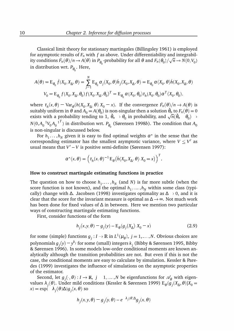
Classical limit theory for stationary martingales (Billingsley 1961) is employedfor asymptotic results of Fn with f as above. Under differentiability and integrabil-ity conditions Fn(θ)=n! A(θ) in Pθ0
-probability for all θ and Fn(θ0)=pn! N(0;V0)in distribution wrt. Pθ0
. Here,
A(θ) = Eθ0f (X0;X∆;θ) = N
∑j=1
Eθ0α j(X0;θ)h j(X0;X∆;θ) = Eθ0
α(X0;θ)h(X0;X∆;θ)V0 = Eθ0
f (X0;X∆;θ0) f (X0;X∆;θ0)T = Eθ0α(X0;θ0)τh(X0;θ0)αT (X0;θ0);
where τh(x;θ) = Varθ (h(X0;X∆;θ)jX0 = x). If the convergence Fn(θ)=n ! A(θ) is
suitably uniform in θ and A0 = A(θ0) is non-singular then a solution θn to Fn(θ) = 0exists with a probability tending to 1, θn ! θ0 in probability, and
pn(θn θ0)!
N(0;A10 V0A1
0T ) in distribution wrt. Pθ0
(Sørensen 1998b). The condition that A0
is non-singular is discussed below.For h1 : : : ;hN given it is easy to find optimal weights α? in the sense that the
corresponding estimator has the smallest asymptotic variance, where V V 0 asusual means that V 0V is positive semi-definite (Sørensen 1997):
α?(x;θ) = τh(x;θ)1Eθh(X0;X∆;θ)jX0 = x
T :How to construct martingale estimating functions in practice
The question on how to choose h1; : : : ;hN (and N) is far more subtle (when thescore function is not known), and the optimal h1; : : : ;hN within some class (typi-cally) change with ∆. Jacobsen (1998) investigates optimality as ∆ ! 0, and it isclear that the score for the invariant measure is optimal as ∆!∞. Not much workhas been done for fixed values of ∆ in between. Here we mention two particularways of constructing martingale estimating functions.
First, consider functions of the form
h j(x;y;θ) = g j(y)Eθ (g j(X∆)jX0 = x) (2.9)
for some (simple) functions g j : I ! R in L1(µθ ), j = 1; : : : ;N. Obvious choices are
polynomials g j(y)= yk j for some (small) integers k j (Bibby & Sørensen 1995, Bibby& Sørensen 1996). In some models low-order conditional moments are known an-alytically although the transition probabilities are not. But even if this is not thecase, the conditional moments are easy to calculate by simulation. Kessler & Pare-des (1999) investigates the influence of simulations on the asymptotic propertiesof the estimator.
Second, let g j(;θ) : I ! R, j = 1; : : : ;N be eigenfunctions for Aθ with eigen-values λ j(θ). Under mild conditions (Kessler & Sørensen 1999) Eθ (g j(X∆;θ)jX0 =x) = exp(λ j(θ)∆)g j(x;θ) so
h j(x;y;θ) = g j(y;θ) eλ j(θ )∆g j(x;θ)
2.3. Estimating functions 11
satisfies (2.8). Note that this h j has the same form as (2.9) except that g j dependson θ . The estimating functions based on eigenfunctions have two advantages:they are invariant to twice continuously differentiable transformations of data andthe optimal weights are easy to simulate (Sørensen 1997). However, the applica-bility is rather limited as the eigenfunctions are known only for a few models; seeKessler & Sørensen (1999) for some non-trivial examples, though.
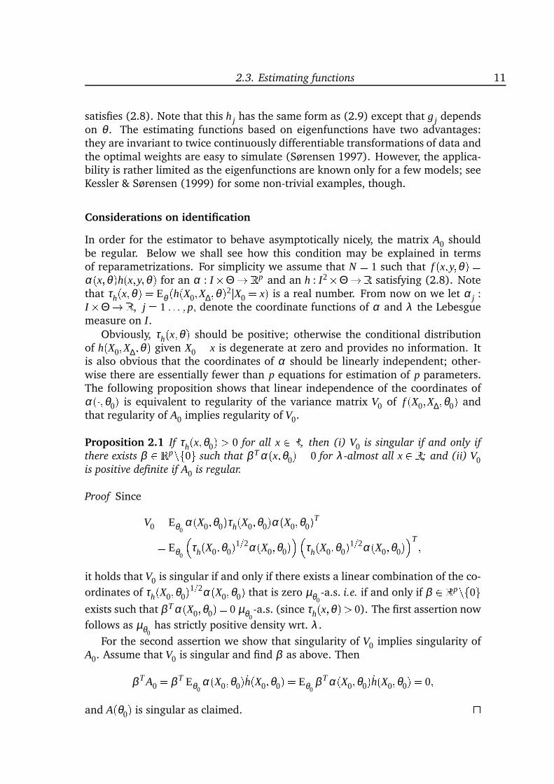
Considerations on identification
In order for the estimator to behave asymptotically nicely, the matrix A0 shouldbe regular. Below we shall see how this condition may be explained in termsof reparametrizations. For simplicity we assume that N = 1 such that f (x;y;θ) =α(x;θ)h(x;y;θ) for an α : IΘ ! Rp and an h : I2Θ ! R satisfying (2.8). Notethat τh(x;θ) = Eθ (h(X0;X∆;θ)2jX0 = x) is a real number. From now on we let α j :IΘ ! R, j = 1 : : : ; p; denote the coordinate functions of α and λ the Lebesguemeasure on I.
Obviously, τh(x;θ) should be positive; otherwise the conditional distributionof h(X0;X∆;θ) given X0 = x is degenerate at zero and provides no information. Itis also obvious that the coordinates of α should be linearly independent; other-wise there are essentially fewer than p equations for estimation of p parameters.The following proposition shows that linear independence of the coordinates ofα(;θ0) is equivalent to regularity of the variance matrix V0 of f (X0;X∆;θ0) andthat regularity of A0 implies regularity of V0.
Proposition 2.1 If τh(x;θ0) > 0 for all x 2 R, then (i) V0 is singular if and only if
there exists β 2 Rpnf0g such that β T α(x;θ0) = 0 for λ -almost all x 2 R; and (ii) V0is positive definite if A0 is regular.
Proof Since
V0 = Eθ0α(X0;θ0)τh(X0;θ0)α(X0;θ0)T= Eθ0
τh(X0;θ0)1=2α(X0;θ0)τh(X0;θ0)1=2α(X0;θ0)T ;
it holds that V0 is singular if and only if there exists a linear combination of the co-
ordinates of τh(X0;θ0)1=2α(X0;θ0) that is zero µθ0-a.s. i.e. if and only if β 2 Rpnf0g
exists such that β T α(X0;θ0) = 0 µθ0-a.s. (since τh(x;θ)> 0). The first assertion now
follows as µθ0has strictly positive density wrt. λ .
For the second assertion we show that singularity of V0 implies singularity ofA0. Assume that V0 is singular and find β as above. Then
β T A0 = β T Eθ0α(X0;θ0)h(X0;θ0) = Eθ0
β T α(X0;θ0)h(X0;θ0) = 0;and A(θ0) is singular as claimed.

12 Chapter 2. Inference for diffusion processes
In the following we shall only consider h of the form h(x;y;θ) = g(y)G(x;θ)where G(x;θ) = Eθ (g(X∆)jX0 = x), see (2.9). Since α is nothing but a weight func-tion, a natural requirement is that G determines the full parameter vector uniquely.In essence, the proposition below claims that this is also sufficient in order for thematrix A?
0 corresponding to the optimal weight function α? =G=τh to be regular.
Below we write Aα0 to stress the dependence of α on A0. In particular, A?
0 = Aα?0 .
We need some further terminology: say that a bijective transformation γ from aneighbourhood Θ0 of θ0 to a set Γ0 Rp is a reparametrization around θ0. Theinverse of γ is denoted by γ1 or θ , and γ0 = γ(θ0). The function Gγ : IΓ0 isdefined by Gγ(x;γ) = G(x;θ(γ)); hence G(x;θ) = Gγ(x;γ(θ)).Proposition 2.2 If there exist j1; : : : ; jq f1; : : : ; pg with jk 6= jk0 for k 6= k0 and a
reparametrization around θ0 such that for j = j1; : : : ; jq
∂Gγ(x;γ0)=∂γ j = 0; λ a:s:; (2.10)
then Aα0 has rank at most q for any α. Conversely, if A?
0 = Aα?0 corresponding to
the optimal α? has rank q < p and τh(x;θ) > 0 for all x 2 I then there exists a
reparametrization γ around θ0 such that (2.10) holds for all j = q+1; : : : ; p.
Proof By the chain rule it holds for any α that
Aα0 =Eθ0
α(X0;θ0)G(X0;θ0)=Eθ0α(X0;θ0)Gγ(X0;γ0)γ(θ0)=Eθ0α(X0;θ0)Gγ(X0;γ0)γ(θ0)
where Gγ is the matrix of derivatives wrt. γ of Gγ and γ is the matrix of derivativesof γ wrt. θ . By assumption the jk’th column of Gγ(X0;γ0) has all elements equal tozero almost surely, k = 1; : : : ;q, so Aα
0 has rank at most q as claimed.For the second assertion, assume that
A?0 = Eθ0
G(X0;θ0)T G(X0;θ0)=τh(X0;θ0)= Eθ0
G(X0;θ0)τh(X0;θ0)1=2T
G(X0;θ0)τh(X0;θ0)1=2has rank q < p and assume without loss of generality that the upper left qq sub-matrix is positive definite (possibly after the coordinates of θ have been renum-bered).
According to Lemma 2.3 below, x1; : : : ;xq exist such that0B ∂G(x1;θ0)=∂θ1 ∂G(x1;θ0)=∂θq...
...∂G(xq;θ0)=∂θ1 ∂G(xq;θ0)=∂θq
1CAis regular. Hence, there is a neighbourhood Θ0 of θ0 such that γ : Θ0! Rp definedby
γ(θ) = G(x1;θ); : : : ;G(xq;θ);θq+1; : : : ;θp
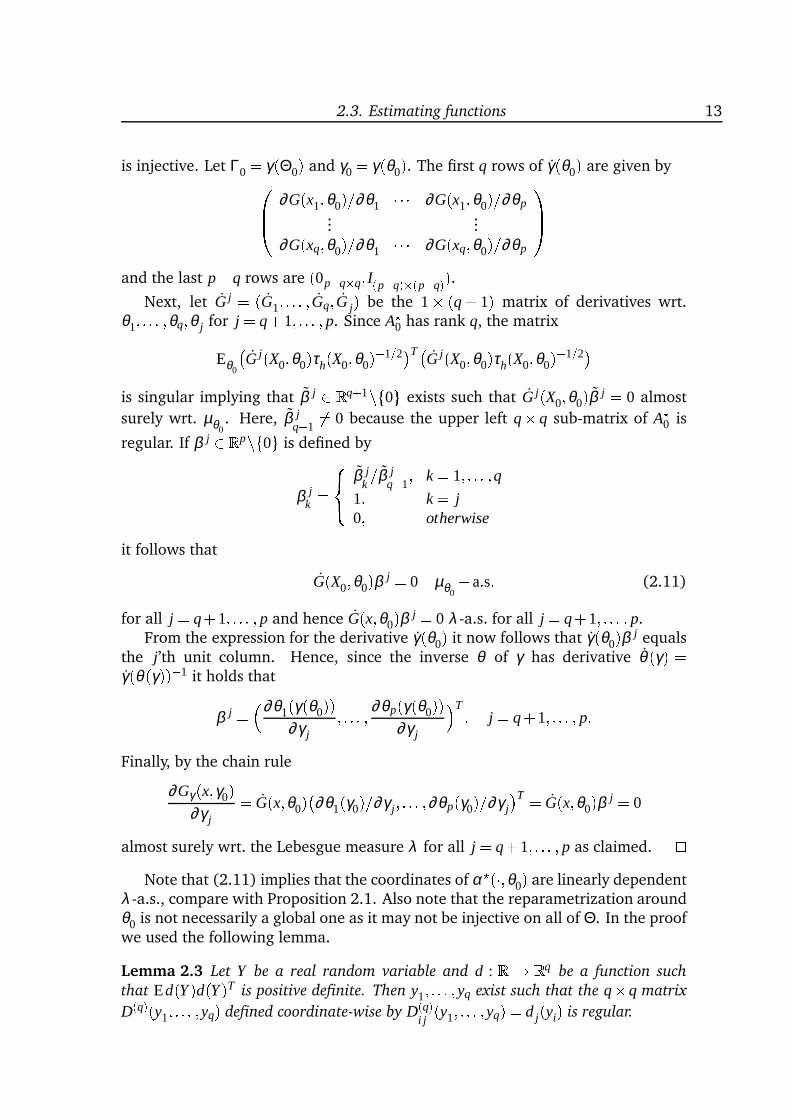
2.3. Estimating functions 13
is injective. Let Γ0 = γ(Θ0) and γ0 = γ(θ0). The first q rows of γ(θ0) are given by0B ∂G(x1;θ0)=∂θ1 ∂G(x1;θ0)=∂θp...
...∂G(xq;θ0)=∂θ1 ∂G(xq;θ0)=∂θp
1CAand the last pq rows are (0pqq; I(pq)(pq)).
Next, let G j = (G1; : : : ; Gq; G j) be the 1 (q + 1) matrix of derivatives wrt.θ1; : : : ;θq;θ j for j = q+1; : : : ; p. Since A?
0 has rank q, the matrix
Eθ0
G j(X0;θ0)τh(X0;θ0)1=2T
G j(X0;θ0)τh(X0;θ0)1=2is singular implying that β j 2 Rq+1nf0g exists such that G j(X0;θ0)β j = 0 almost
surely wrt. µθ0. Here, β j
q+16= 0 because the upper left q q sub-matrix of A?
0 is
regular. If β j 2 Rpnf0g is defined by
β jk=8<: β j
k=β j
q+1; k = 1; : : : ;q
1; k = j0; otherwise
it follows that
G(X0;θ0)β j = 0 µθ0a:s: (2.11)
for all j = q+1; : : : ; p and hence G(x;θ0)β j = 0 λ -a.s. for all j = q+1; : : : ; p.From the expression for the derivative γ(θ0) it now follows that γ(θ0)β j equals
the j’th unit column. Hence, since the inverse θ of γ has derivative θ (γ) =γ(θ(γ))1 it holds that
β j = ∂θ1(γ(θ0))∂γ j
; : : : ; ∂θp(γ(θ0))∂γ j
T ; j = q+1; : : : ; p:Finally, by the chain rule
∂Gγ(x;γ0)∂γ j
= G(x;θ0)∂θ1(γ0)=∂γ j; : : : ;∂θp(γ0)=∂γ j
T = G(x;θ0)β j = 0
almost surely wrt. the Lebesgue measure λ for all j = q+1; : : : ; p as claimed. Note that (2.11) implies that the coordinates of α?(;θ0) are linearly dependent
λ -a.s., compare with Proposition 2.1. Also note that the reparametrization aroundθ0 is not necessarily a global one as it may not be injective on all of Θ. In the proofwe used the following lemma.
Lemma 2.3 Let Y be a real random variable and d : R ! Rq be a function such
that Ed(Y )d(Y)T is positive definite. Then y1; : : : ;yq exist such that the q q matrix
D(q)(y1; : : : ;yq) defined coordinate-wise by D(q)i j
(y1; : : : ;yq) = d j(yi) is regular.
14 Chapter 2. Inference for diffusion processes
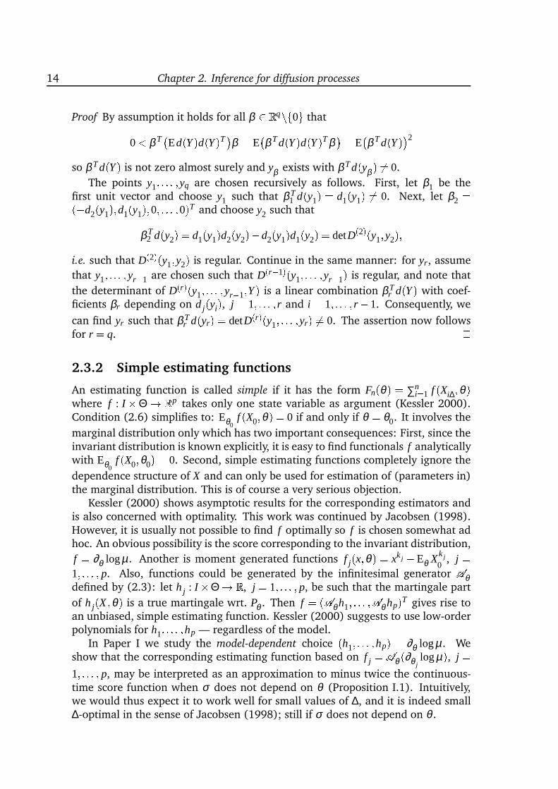
Proof By assumption it holds for all β 2 Rqnf0g that
0< β TEd(Y )d(Y)Tβ = Eβ T d(Y )d(Y)T β
= Eβ T d(Y)2
so β T d(Y ) is not zero almost surely and yβ exists with β T d(yβ ) 6= 0.
The points y1; : : : ;yq are chosen recursively as follows. First, let β1 be thefirst unit vector and choose y1 such that β T
1 d(y1) = d1(y1) 6= 0. Next, let β2 =(d2(y1);d1(y1);0; : : : ;0)T and choose y2 such that
β T2 d(y2) = d1(y1)d2(y2)d2(y1)d1(y2) = detD(2)(y1;y2);
i.e. such that D(2)(y1;y2) is regular. Continue in the same manner: for yr, assume
that y1; : : : ;yr1 are chosen such that D(r1)(y1; : : : ;yr1) is regular, and note that
the determinant of D(r)(y1; : : : ;yr1;Y ) is a linear combination β Tr d(Y) with coef-
ficients βr depending on d j(yi), j = 1; : : : ;r and i = 1; : : : ;r1. Consequently, we
can find yr such that β Tr d(yr) = detD(r)(y1; : : : ;yr) 6= 0. The assertion now follows
for r = q. 2.3.2 Simple estimating functions
An estimating function is called simple if it has the form Fn(θ) = ∑ni=1 f (Xi∆;θ)
where f : IΘ ! Rp takes only one state variable as argument (Kessler 2000).Condition (2.6) simplifies to: Eθ0
f (X0;θ) = 0 if and only if θ = θ0. It involves the
marginal distribution only which has two important consequences: First, since theinvariant distribution is known explicitly, it is easy to find functionals f analyticallywith Eθ0
f (X0;θ0) = 0. Second, simple estimating functions completely ignore the
dependence structure of X and can only be used for estimation of (parameters in)the marginal distribution. This is of course a very serious objection.
Kessler (2000) shows asymptotic results for the corresponding estimators andis also concerned with optimality. This work was continued by Jacobsen (1998).However, it is usually not possible to find f optimally so f is chosen somewhat adhoc. An obvious possibility is the score corresponding to the invariant distribution,
f = ∂θ logµ. Another is moment generated functions f j(x;θ) = xk j Eθ X k j0
, j =1; : : : ; p. Also, functions could be generated by the infinitesimal generator Aθdefined by (2.3): let h j : IΘ ! R, j = 1; : : : ; p, be such that the martingale part
of h j(X ;θ) is a true martingale wrt. Pθ . Then f = (Aθ h1; : : : ;Aθ hp)T gives rise toan unbiased, simple estimating function. Kessler (2000) suggests to use low-orderpolynomials for h1; : : : ;hp — regardless of the model.
In Paper I we study the model-dependent choice (h1; : : : ;hp) = ∂θ logµ. Weshow that the corresponding estimating function based on f j =Aθ (∂θ j
logµ), j =1; : : : ; p, may be interpreted as an approximation to minus twice the continuous-time score function when σ does not depend on θ (Proposition I.1). Intuitively,we would thus expect it to work well for small values of ∆, and it is indeed small∆-optimal in the sense of Jacobsen (1998); still if σ does not depend on θ .
2.3. Estimating functions 15
There are two important differences from the usual Riemann-Itô approxima-tion of the continuous-time score, that is, the logarithmic derivative wrt. θ of(2.5): the above approximation is unbiased which the Riemann-Itô approxima-tion is not; and each term in the Riemann-Itô approximation depends on pairs ofobservations whereas each term in the above approximation depends on a singleobservation only.
Also note that the estimating function from Paper I is invariant to bijective andtwice differentiable transformations of the data if σ does not depend on θ (Propo-sition I.2); this is not the case for the simple estimating functions discussed earlier.The ideas carry over (to some extent at least) to multi-dimensional diffusions, andthe estimating function works quite well in simulation studies.
Finally, a remark connecting a simple estimating function Fn(θ) = ∑ni=1 f (Xi∆;θ)
to a class of martingale estimating functions. Define
h f (x;y;θ) =Uθ f (y;θ) Uθ f (x;θ) f (x;θ)where Uθ is the potential operator given by Uθ f (x;θ) = ∑∞
k=0Eθ ( f (Xk∆;θ)jX0 =x). Then h f satisfies condition (2.8), and the martingale estimating functions
∑ni=1h f (X(i1)∆;Xi∆;θ) and Fn(θ) are asymptotically equivalent (Jacobsen 1998).
However, the martingale estimating function may be improved by introducingweights α (unless of course the optimal weight α?(;θ) is constant). In this sensemartingale estimating functions are always better (or at least as good) as simpleestimating functions. In practice it is not very helpful, though, as the potentialoperator in general is not known! Also, the improvement may be very small as weshall see in the following example.
Example (The Ornstein-Uhlenbeck process) Consider the solution to dXt = θXt dt +dWt where θ < 0. Kessler (2000) shows that the optimal simple estimating functionis obtained for f (x;θ) = 2θx2+1. It is easy to see that h f (x;y;θ)∝ f (y;θ)ψ f (x;θ)where ψ = ψ(θ ;∆) = exp(2θ∆) and that the optimal weight function is given by
α?(x;θ) = Eθh f (X0;X∆)jX0 = x
τh f
(x;θ) = 4θ∆ψx2 (1ψ +2θ∆ψ)=θ8θψ(1ψ)x2+2(1ψ)2 :Since α?(;θ) is not constant, improvement is indeed possible. It turns out, how-ever, that the asymptotic variance is only reduced by about 1% (for θ0 =1).
It is well-known that the optimal simple estimating function is nearly (globally)efficient in the Ornstein-Uhlenbeck model, and the example does not rule outthe possibility that the improvement could be considerable for other models (andother simple estimating functions).
2.3.3 Comments
Obviously, there are lots of unbiased estimating functions that are neither martin-gales nor simple. For example,
f (x;y;θ) = h2(y;θ)Aθ h1(x;θ)h1(x;θ)Aθ h2(y;θ)
16 Chapter 2. Inference for diffusion processes
generates a class of estimating functions which are transition dependent and yetexplicit (Hansen & Scheinkman 1995, Jacobsen 1998).
Estimating functions of different kinds may of course be combined. For ex-ample, one could firstly estimate parameters from the invariant distribution bysolving a simple estimating equation and secondly estimate parameters from theconditional distribution one step ahead. See Bibby & Sørensen (1998) for a suc-cesful application.
Also, estimating functions may be used as building blocks for the generalized
method of moments (GMM), the much favored estimation method in the econo-metric literature (Hansen 1982). Estimation via GMM is essentially performedby choosing an estimating function Fn of dimension p0 > p and minimizing thequadratic form Fn(θ)T ΩFn(θ) for some weight matrix Ω.
2.4 Approximate maximum likelihood estimation
We now describe three approximate maximum likelihood methods. They all sup-ply approximations, analytical or numerical, of pθ (∆;x; ) for fixed x and θ . Inparticular they supply approximations of pθ (∆;X(i1)∆;Xi∆), i = 1; : : : ;n, and there-
fore of Ln(θ). The approximate likelihood is finally maximized over θ 2Θ.
2.4.1 An analytical approximation
A naive, explicit approximation of the conditional distribution of X∆ given X0 = xis provided by the Euler approximation. The Gaussian approximation may be pooreven if the conditional moments are replaced by accurate approximations (or per-haps even the true moments). A sequence of explicit, non-Gaussian approximations
of pθ (∆;x; ) is suggested by Aït-Sahalia (1998). For fixed x and θ the idea is to(i) transform X to a process Z which, conditional on X0 = x, has Z0 = 0 and Z∆“close” to standard normal; (ii) define a truncated Hermite series expansion ofthe density of Z∆ around the standard normal density; and (iii) invert the Hermiteapproximation in order to obtain an approximation of pθ (∆;x; ).
For step (i) define Z = gx;θ (X) where
gx;θ (y) = 1p∆
Z y
x
1σ(u;θ) du:
Then Z solves dZt = bZ(Zt ;θ)dt +1=p∆dWt with drift function given by Itô’s for-
mula and Z0 = 0 (given X0 = x). Note that g0x;θ (y) = (∆σ2(y;θ))1=2 > 0 for all y 2 Iso that gx;θ is injective.
For step (ii) note that N(0;1) is a natural approximation of the conditionaldistribution of Z∆ given Z0 = 0, as increments of Z over time intervals of length ∆has approximately unit variance. Let pZ
θ (∆;0; ) denote the true conditional densityof Z∆ given Z0 = 0 and let pZ;J
θ (∆;0; ) be the Hermite series expansion truncated after
J terms of pZθ (∆;0; ) around the standard normal density.
2.4. Approximate maximum likelihood estimation 17
For step (iii) note that the true densities pθ (∆;x; ) and pZθ (∆;0; ) are related by
pθ (∆;x;y) = 1p∆σ(x;θ) pZ
θ∆;0;gx;θ(y); y 2 I
and apply this formula to invert the approximation pZ;Jθ (∆;0; ) of pZ
θ (∆;0; ) into an
approximation pJθ (∆;x; ) of pθ (∆;x; ) in the natural way:
pJθ (∆;x;y) = 1p
∆σ(x;θ) pZ;Jθ∆;0;gx;θ (y); y 2 I:
Then pJθ (∆;x;y) converges to pθ (∆;x;y) as J !∞, suitably uniformly in y and θ .
Furthermore, if J = J(n) tends to infinity fast enough as n! ∞ then the estimatormaximizing ∏n
i=1 pJ(n)θ (∆;X(i1)∆;Xi∆) is asymptotically equivalent to the maximum
likelihood estimator (Aït-Sahalia 1998, Theorems 1 and 2).Note that the coefficients of the Hermite series expansion cannot be computed
explicitly but could be replaced by analytical approximations in terms of the in-finitesimal generator. Hence, the technique provides explicit, though very complex,approximations to pθ (∆;x; ). Aït-Sahalia (1998) performs numerical experimentsthat indicate that the error pJ
θ (∆;x;y) pθ (∆;x;y) decreases quickly; roughly witha factor 10 for each extra term included in the expansion of pZ
θ (∆;0; ).2.4.2 Numerical solutions of the Kolmogorov forward equation
A classical result from stochastic calculus states that the transition densities undercertain regularity conditions are characterized as solutions to the Kolmogorov for-
ward equations. Lo (1988) employs a similar result and finds explicit expressionsfor the likelihood function for a log-normal diffusion with jumps and a Brownianmotion with zero as an absorbing state. Poulsen (1999) seems to be the first toemploy numerical procedures for non-trivial diffusion models.
For x and θ fixed the forward equation for pθ (;x; ) is a partial differentialequation: for (t;y) 2 (0;∞) I,
∂∂ t
pθ (t;x;y) = ∂∂y
b(y;θ)pθ (t;x;y)+ 1
2∂ 2
∂ (y)2
σ2(y;θ)pθ (t;x;y);
with initial condition pθ (0;x;y) = δ (x y) where δ is the Dirac delta function. Inorder to calculate the likelihood Ln(θ) one has to solve n of the above forwardequations, one for each X(i1)∆, i = 1; : : : ;n. Note that the forward equation for
X(i1)∆ determines pθ (t;X(i1)∆;y) for all values of (t;y), but that we only need it at
a single point, namely (∆;Xi∆).Poulsen (1999) employs the so-called Crank-Nicholson finite difference meth-
od for each of the n forward equations. For fixed θ he obtains a second orderapproximation of logLn(θ) in the sense that the numerical approximation logLh
n(θ)satisfies
logLhn(θ) = logLn(θ)+h2 f θ
n (X0;X∆; : : : ;Xn∆)+o(h2)gθn (X0;X∆; : : : ;Xn∆)
18 Chapter 2. Inference for diffusion processes
for suitable functions f θn and gθ
n . The parameter h determines how fine-grained a(t;y)-grid used in the numerical procedure is (and thus the accuracy of approxi-mation). If h = h(n) tends to zero faster than n1=4 as n ! ∞ then the estimatormaximizing logLh
n(θ) is asymptotically equivalent to the maximum likelihood esti-mator (Poulsen 1999, Theorem 3).
Poulsen (1999) fits the CKLS model to a dataset of 655 observations (in arevised version, even a six-parameter extension is fitted) and is able to do it inquite reasonable time. Although n partial differential equations must be solvedthe method seems to be much faster than the simulation based method below.
2.4.3 Approximation via simulation
Pedersen (1995b) defines a sequence of approximations to pθ (∆;x; ) via a missingdata approach. The basic idea is to (i) split the time interval from 0 to ∆ into piecesshort enough that the Euler approximation holds reasonably well; (ii) considerthe joint Euler likelihood for the augmented data consisting of the observationX∆ and the values of X at the endpoints of the subintervals; (iii) integrate theunobserved variable out of the joint Euler density; and (iv) calculate the resultingexpectation by simulation. The method has been applied successfully to the CKLSmodel (Honoré 1997).
To be precise, let x and θ be fixed, consider an integer N 0, and split theinterval [0;∆ into N +1 subintervals of length ∆N = ∆=(N +1). Use the notationX0;k for the (unobserved) value of X at time k=(N + 1), k = 1; : : : ;N. Then (with
x0;0 = x and x0;N+1 = y),
pθ (∆;x;y) = ZIN
N+1
∏i=1
pθ∆N ;x0;i1;x0;id(x0;1; : : : ;x0;N)= Z
IpθN∆N ;x;x0;Npθ
∆N;x0;N ;ydx0;N= Eθ
pθ∆N;X0;N;yX0 = x
; y 2 I (2.12)
where we have used the Chapman-Kolmogorov equations.Now, for ∆N small (N large), pθ (∆N ;x0;N; ) is well approximated by the normal
density with mean x0;N +b(x0;N ;θ)∆N and variance σ2(x0;N;θ)∆N. Let pNθ (∆N;x0;N; )
denote this density. Following (2.12),
pNθ (∆;x;y) = Eθ
pN
θ∆N;X0;N;yX0 = x
is a natural approximation of pθ (∆;x;y), y 2 I. Note that N = 0 corresponds to thesimple Euler approximation.
The approximate likelihood functions LNn (θ) = ∏n
i=1 pNθ (∆;X(i1)∆;Xi∆) converge
in probability to Ln(θ) as N ! ∞ (Pedersen 1995b, Theorems 3 and 4). Further-more, there exists a sequence N(n) such that the estimator maximizing LN(n)
n (θ)
2.5. Bayesian analysis 19
is asymptotically equivalent (as n ! ∞) to the maximum likelihood estimator(Pedersen 1995a, Theorem 3).
In practice we could calculate pNθ (∆;x;y) as the average of a large number of
values fpNθ (∆;X r
0;N;y)gr where X r0;N is the last element of a simulated discrete-time
path X0;X r0;1; : : : ;X r
0;N started at x. Note that the paths are simulated conditionalon X0 = x only which implies that the simulated values X r
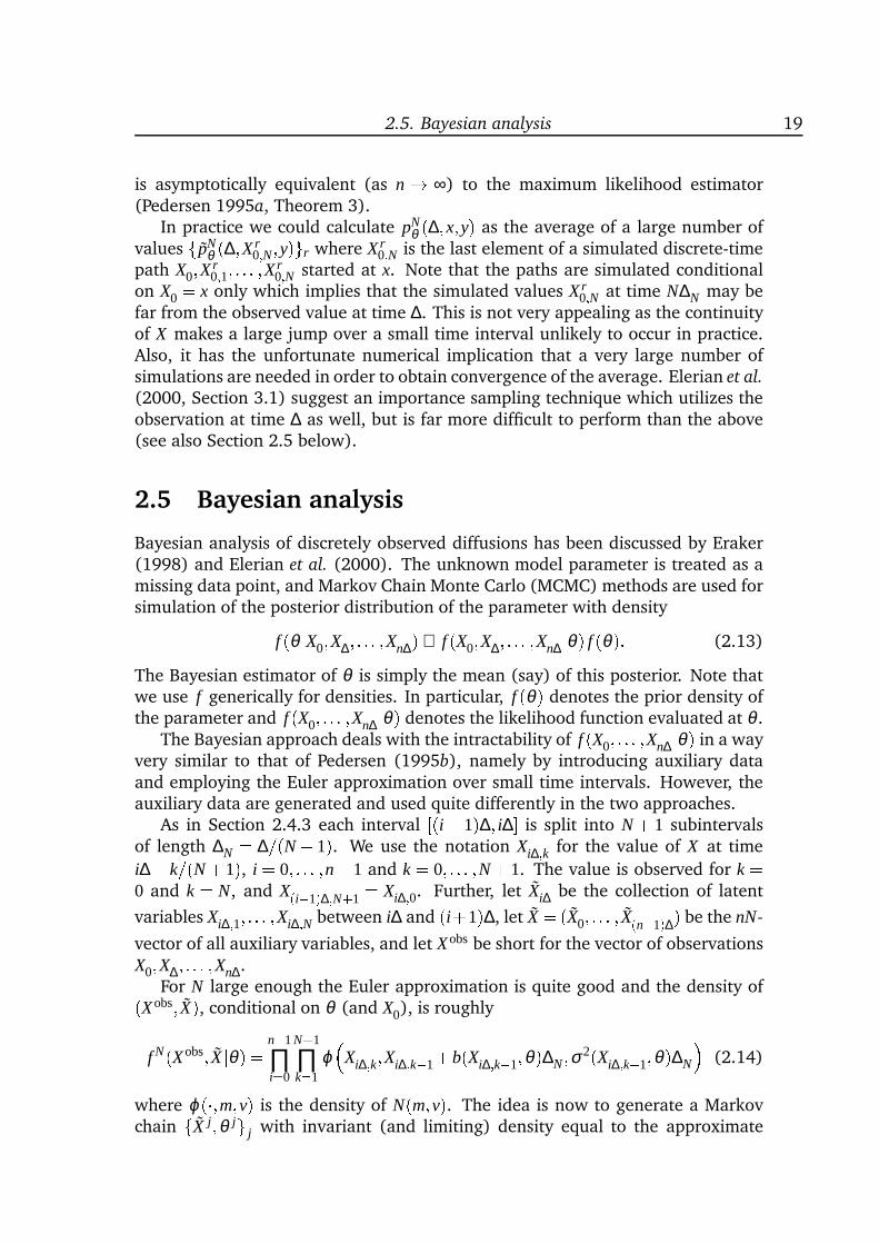
0;N at time N∆N may befar from the observed value at time ∆. This is not very appealing as the continuityof X makes a large jump over a small time interval unlikely to occur in practice.Also, it has the unfortunate numerical implication that a very large number ofsimulations are needed in order to obtain convergence of the average. Elerian et al.
(2000, Section 3.1) suggest an importance sampling technique which utilizes theobservation at time ∆ as well, but is far more difficult to perform than the above(see also Section 2.5 below).
2.5 Bayesian analysis
Bayesian analysis of discretely observed diffusions has been discussed by Eraker(1998) and Elerian et al. (2000). The unknown model parameter is treated as amissing data point, and Markov Chain Monte Carlo (MCMC) methods are used forsimulation of the posterior distribution of the parameter with density
f (θ jX0;X∆; : : : ;Xn∆) ∝ f (X0;X∆; : : : ;Xn∆jθ) f (θ): (2.13)
The Bayesian estimator of θ is simply the mean (say) of this posterior. Note thatwe use f generically for densities. In particular, f (θ) denotes the prior density ofthe parameter and f (X0; : : : ;Xn∆jθ) denotes the likelihood function evaluated at θ .
The Bayesian approach deals with the intractability of f (X0; : : : ;Xn∆jθ) in a wayvery similar to that of Pedersen (1995b), namely by introducing auxiliary dataand employing the Euler approximation over small time intervals. However, theauxiliary data are generated and used quite differently in the two approaches.
As in Section 2.4.3 each interval [(i 1)∆; i∆ is split into N + 1 subintervalsof length ∆N = ∆=(N + 1). We use the notation Xi∆;k for the value of X at time
i∆+ k=(N +1), i = 0; : : : ;n1 and k = 0; : : : ;N +1. The value is observed for k =0 and k = N, and X(i1)∆;N+1 = Xi∆;0. Further, let Xi∆ be the collection of latent
variables Xi∆;1; : : : ;Xi∆;N between i∆ and (i+1)∆, let X = (X0; : : : ; X(n1)∆) be the nN-
vector of all auxiliary variables, and let Xobs be short for the vector of observationsX0;X∆; : : : ;Xn∆.
For N large enough the Euler approximation is quite good and the density of(Xobs; X), conditional on θ (and X0), is roughly
f N(Xobs; X jθ) = n1
∏i=0
N+1
∏k=1
ϕ
Xi∆;k;Xi∆;k1+b(Xi∆;k1;θ)∆N;σ2(Xi∆;k1;θ)∆N
(2.14)
where ϕ(;m;v) is the density of N(m;v). The idea is now to generate a Markovchain fX j;θ jg j with invariant (and limiting) density equal to the approximate
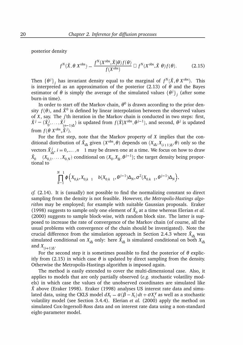
20 Chapter 2. Inference for diffusion processes
posterior density
f N(X;θ jXobs) = f N(Xobs; X jθ) f (θ)f (Xobs) ∝ f N(Xobs; X jθ) f (θ): (2.15)
Then fθ jg j has invariant density equal to the marginal of f N(X ;θ jXobs). Thisis interpreted as an approximation of the posterior (2.13) of θ and the Bayesestimator of θ is simply the average of the simulated values fθ jg j (after someburn-in time).
In order to start off the Markov chain, θ0 is drawn according to the prior den-sity f (θ), and X0 is defined by linear interpolation between the observed valuesof X , say. The j’th iteration in the Markov chain is conducted in two steps: first,X j = (X j
0; : : : ; X j(n1)∆) is updated from f (X jXobs;θ j1), and second, θ j is updated
from f (θ jXobs; X j).For the first step, note that the Markov property of X implies that the con-
ditional distribution of Xi∆ given (Xobs;θ) depends on (Xi∆;X(i+1)∆;θ) only so the
vectors X ji∆, i = 0; : : : ;n1 may be drawn one at a time. We focus on how to draw
X0 = (X0;1; : : : ;X0;N) conditional on (X0;X∆;θ j1); the target density being propor-tional to
N+1
∏k=1
ϕ
X0;k;X0;k1+b(X0;k1;θ j1)∆N;σ2(X0;k1;θ j1)∆N
;cf. (2.14). It is (usually) not possible to find the normalizing constant so directsampling from the density is not feasible. However, the Metropolis-Hastings algo-
rithm may be employed; for example with suitable Gaussian proposals. Eraker(1998) suggests to sample only one element of X0 at a time whereas Elerian et al.
(2000) suggests to sample block-wise, with random block size. The latter is sup-posed to increase the rate of convergence of the Markov chain (of course, all theusual problems with convergence of the chain should be investigated). Note thecrucial difference from the simulation approach in Section 2.4.3 where Xi∆ wassimulated conditional on Xi∆ only: here Xi∆ is simulated conditional on both Xi∆and X(i+1)∆.
For the second step it is sometimes possible to find the posterior of θ explic-itly from (2.15) in which case θ is updated by direct sampling from the density.Otherwise the Metropolis-Hastings algorithm is imposed again.
The method is easily extended to cover the multi-dimensional case. Also, itapplies to models that are only partially observed (e.g. stochastic volatility mod-els) in which case the values of the unobserved coordinates are simulated likeX above (Eraker 1998). Eraker (1998) analyses US interest rate data and simu-lated data, using the CKLS model dXt = α(β Xt)dt +σX γ
t as well as a stochasticvolatility model (see Section 3.4.4). Elerian et al. (2000) apply the method onsimulated Cox-Ingersoll-Ross data and on interest rate data using a non-standardeight-parameter model.
2.6. Estimation based on auxiliary models 21
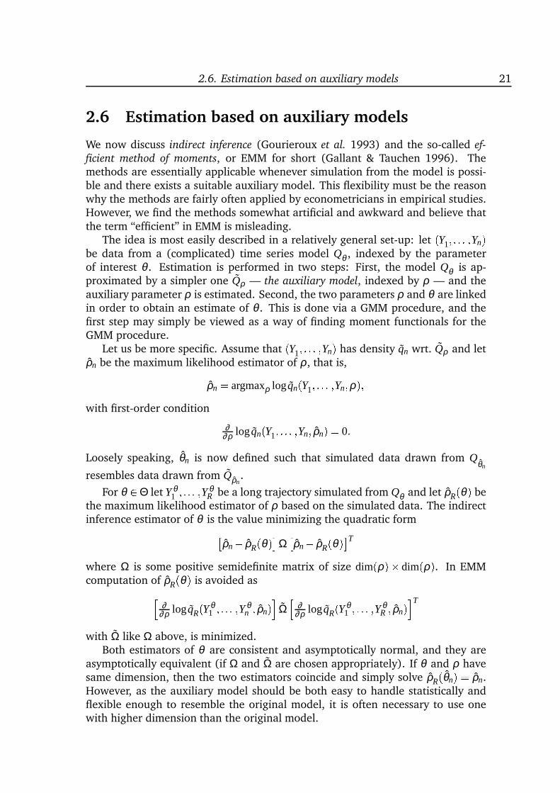
2.6 Estimation based on auxiliary models
We now discuss indirect inference (Gourieroux et al. 1993) and the so-called ef-
ficient method of moments, or EMM for short (Gallant & Tauchen 1996). Themethods are essentially applicable whenever simulation from the model is possi-ble and there exists a suitable auxiliary model. This flexibility must be the reasonwhy the methods are fairly often applied by econometricians in empirical studies.However, we find the methods somewhat artificial and awkward and believe thatthe term “efficient” in EMM is misleading.
The idea is most easily described in a relatively general set-up: let (Y1; : : : ;Yn)be data from a (complicated) time series model Qθ , indexed by the parameterof interest θ . Estimation is performed in two steps: First, the model Qθ is ap-proximated by a simpler one Qρ — the auxiliary model, indexed by ρ — and theauxiliary parameter ρ is estimated. Second, the two parameters ρ and θ are linkedin order to obtain an estimate of θ . This is done via a GMM procedure, and thefirst step may simply be viewed as a way of finding moment functionals for theGMM procedure.
Let us be more specific. Assume that (Y1; : : : ;Yn) has density qn wrt. Qρ and letρn be the maximum likelihood estimator of ρ, that is,
ρn = argmaxρ logqn(Y1; : : : ;Yn;ρ);with first-order condition
∂∂ρ logqn(Y1; : : : ;Yn; ρn) = 0:
Loosely speaking, θn is now defined such that simulated data drawn from Qθn
resembles data drawn from Qρn.
For θ 2Θ let Y θ1 ; : : : ;Y θ
R be a long trajectory simulated from Qθ and let ρR(θ) bethe maximum likelihood estimator of ρ based on the simulated data. The indirectinference estimator of θ is the value minimizing the quadratic form
ρn ρR(θ)Ωρn ρR(θ)T
where Ω is some positive semidefinite matrix of size dim(ρ) dim(ρ). In EMMcomputation of ρR(θ) is avoided ash
∂∂ρ logqR(Y θ
1 ; : : : ;Y θn ; ρn)iΩ
h∂
∂ρ logqR(Y θ1 ; : : : ;Y θ
R ; ρn)iT
with Ω like Ω above, is minimized.Both estimators of θ are consistent and asymptotically normal, and they are
asymptotically equivalent (if Ω and Ω are chosen appropriately). If θ and ρ havesame dimension, then the two estimators coincide and simply solve ρR(θn) = ρn.However, as the auxiliary model should be both easy to handle statistically andflexible enough to resemble the original model, it is often necessary to use onewith higher dimension than the original model.
22 Chapter 2. Inference for diffusion processes
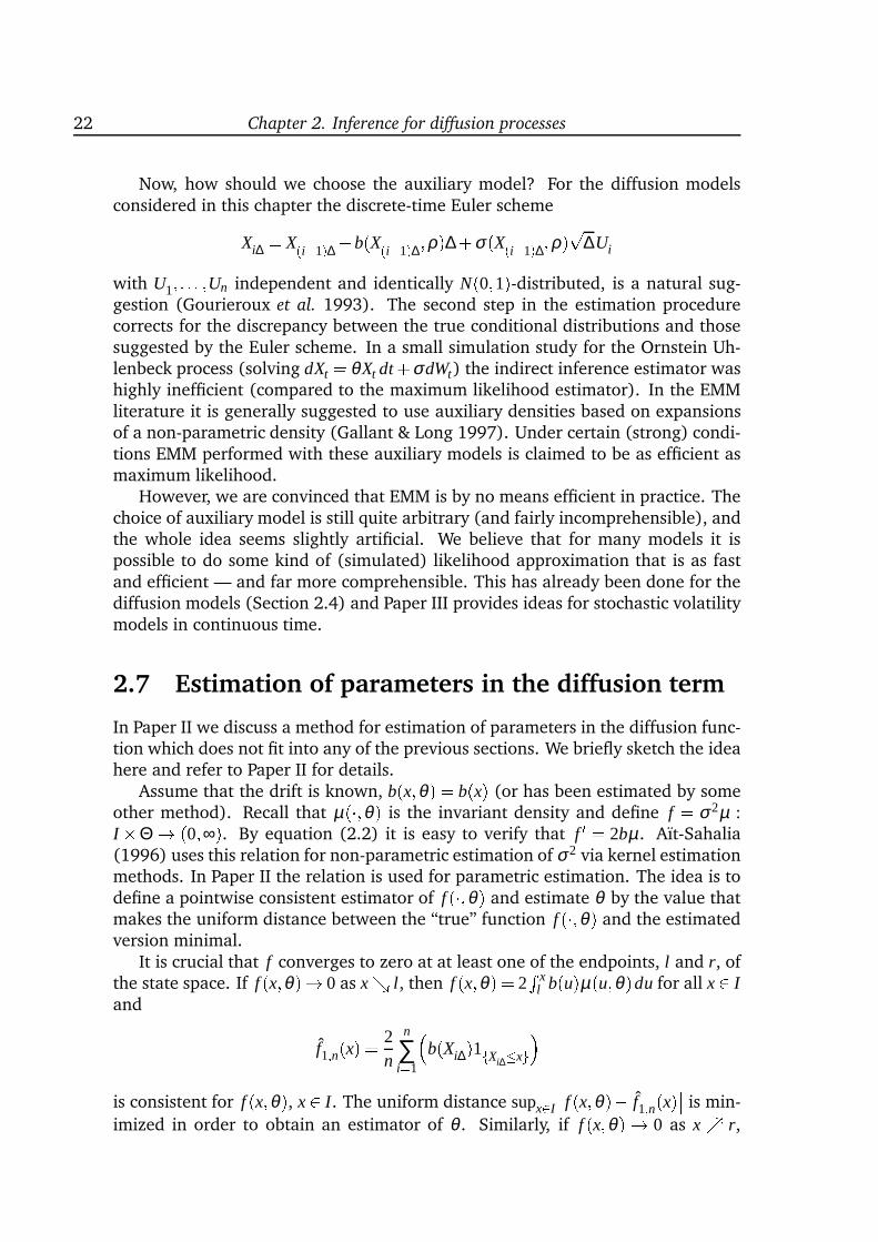
Now, how should we choose the auxiliary model? For the diffusion modelsconsidered in this chapter the discrete-time Euler scheme
Xi∆ = X(i1)∆ +b(X(i1)∆;ρ)∆+σ(X(i1)∆;ρ)p∆Ui
with U1; : : : ;Un independent and identically N(0;1)-distributed, is a natural sug-gestion (Gourieroux et al. 1993). The second step in the estimation procedurecorrects for the discrepancy between the true conditional distributions and thosesuggested by the Euler scheme. In a small simulation study for the Ornstein Uh-lenbeck process (solving dXt = θXt dt +σdWt) the indirect inference estimator washighly inefficient (compared to the maximum likelihood estimator). In the EMMliterature it is generally suggested to use auxiliary densities based on expansionsof a non-parametric density (Gallant & Long 1997). Under certain (strong) condi-tions EMM performed with these auxiliary models is claimed to be as efficient asmaximum likelihood.
However, we are convinced that EMM is by no means efficient in practice. Thechoice of auxiliary model is still quite arbitrary (and fairly incomprehensible), andthe whole idea seems slightly artificial. We believe that for many models it ispossible to do some kind of (simulated) likelihood approximation that is as fastand efficient — and far more comprehensible. This has already been done for thediffusion models (Section 2.4) and Paper III provides ideas for stochastic volatilitymodels in continuous time.
2.7 Estimation of parameters in the diffusion term
In Paper II we discuss a method for estimation of parameters in the diffusion func-tion which does not fit into any of the previous sections. We briefly sketch the ideahere and refer to Paper II for details.
Assume that the drift is known, b(x;θ) = b(x) (or has been estimated by someother method). Recall that µ(;θ) is the invariant density and define f = σ2µ :IΘ ! (0;∞). By equation (2.2) it is easy to verify that f 0 = 2bµ. Aït-Sahalia(1996) uses this relation for non-parametric estimation of σ2 via kernel estimationmethods. In Paper II the relation is used for parametric estimation. The idea is todefine a pointwise consistent estimator of f (;θ) and estimate θ by the value thatmakes the uniform distance between the “true” function f (;θ) and the estimatedversion minimal.
It is crucial that f converges to zero at at least one of the endpoints, l and r, ofthe state space. If f (x;θ)! 0 as x& l, then f (x;θ) = 2
R xl b(u)µ(u;θ)du for all x 2 I
and
f1;n(x) = 2n
n
∑i=1
b(Xi∆)1fXi∆xg
is consistent for f (x;θ), x 2 I. The uniform distance supx2I
f (x;θ) f1;n(x) is min-
imized in order to obtain an estimator of θ . Similarly, if f (x;θ)! 0 as x % r,
2.8. Conclusion 23
then
f2;n(x) =2n
n
∑i=1
b(Xi∆)1fXi∆>xg
is consistent for f (x;θ), x2 I, and supx2I
f (x;θ) f2;n(x) is minimized. If f (x;θ)!0 at both l and r then both f1;n and f2;n provide pointwise consistent estimators
of f (;θ), and we may use a weighted average fn of the two in order to reducevariance.
The estimators arep
n-consistent and in certain cases weakly convergent (The-orems II.7 and II.9) but the limit distribution need not be Gaussian. Note thatthe observations are mixed in a quite complex way in the uniform distance so theusual limit theorems do not apply. Instead, the asymptotic results are proved usingempirical process theory. We are not aware of any other applications of empiricalprocess theory to problems related to inference for diffusion processes.
In Paper II we apply the method to simulated data from the CKLS model, dXt =(α +βXt)dt +σX γt dWt , and get reasonable estimators for both γ and σ . The drift
parameters are estimated beforehand using martingale estimating functions. Notethat this model is relatively hard to identify as different values of the pair (γ;σ)may yield very similar diffusion functions.
There are two objections to the method. First, it provides estimators of theparameters in the diffusion function only; the drift needs to be estimated before-hand. This is possible via martingale estimating functions if the drift is linear (asin many popular models, e.g. the CKLS model above), but is otherwise difficult.Second, the approach is perhaps somewhat ad hoc and the estimators need not beefficient.
2.8 Conclusion
Maximum likelihood estimation is typically not possible for diffusion processesthat have been observed at discrete time-points only. In this chapter we havereviewed a number of alternatives from the literature.
From a classical point of view, the most appealing methods are those basedon approximations of the true likelihood that in principle can be made arbitrarilyaccurate. We reviewed three types above: One provides analytical approximationsto the likelihood function and is therefore in principle the easiest one to use. Theexpressions are quite complicated, though, even for low-order approximations.The other two rely on numerical techniques, one on numerical solutions to partialdifferential equations and one on simulations. Even with today’s efficient comput-ers both methods are quite computationally demanding so faster procedures areoften valuable.
Estimation via estimating functions is generally much faster. So-called simpleestimating functions are available in explicit form but provide only estimators forparameters from the marginal distribution. Still, they may be useful for prelimi-nary analysis. Paper I investigates a special simple estimating function which can
24 Chapter 2. Inference for diffusion processes
be interpreted as an approximation of the continuous-time score function. Thecorresponding estimator is invariant to transformations of data. Martingale esti-mating functions are analytically available for a few models but must in generalbe calculated by simulated. This basically amounts to simulating conditional ex-pectations, which is faster than calculating conditional densities as required bythe direct likelihood approximations above. Under regularity conditions, estima-tors obtained by martingale estimating functions are consistent and asymptoticallynormal. We studied one of the regularity conditions in some detail and showedhow it may be explained in terms of reparametrizations.
The Bayesian approach is to consider the parameter as random and make sim-ulations from its (posterior) distribution. This is quite hard and requires simu-lation, conditional on the observations, of the diffusion process at a number oftime-points in between those where it was observed. The posterior distributiondepends on the prior distribution which is chosen more or less arbitrarily. Indi-rect inference and EMM remove bias due to the discrete-time auxiliary model bysimulation methods. The quality of the estimators is bound to depend on the aux-iliary model which is chosen somewhat arbitrarily, and we believe that more directapproaches are preferable. The procedure from Section 2.7 (and Paper II) for esti-mation of the diffusion parameters (when the drift is known) provides satisfactoryestimates in the difficult CKLS model. The estimators are probably not efficient,though. The application of empirical process theory for proving asymptotic resultsis interesting from a theoretical point of view.
3Stochastic volatility models
In this chapter we discuss continuous-time stochastic volatility models. By thiswe mean two-dimensional diffusion models where only one of the coordinates isobservable and where the stochastic differential equation has a special form. Themodels were introduced in the mathematical finance literature in the late eightiesas modifications of the classical Black-Scholes model. However, only very recentlysatisfactory estimation methods have been developed.
This chapter provides an overview of existing estimation techniques and a com-parison of four specific models. There exist review papers on stochastic volatilitymodels (Ghysels, Harvey & Renault 1996, Shephard 1996), but they are mainlyconcerned with models defined in discrete time. The continuous-time case issomewhat more delicate because not even the distribution of the latent processis known. Hence, not all discrete-time methods can be applied, and those that canare in general more troublesome for continuous-time models.
My main contribution is the development of a new estimation technique rely-ing on simulated approximations to the likelihood. The estimation method is dis-cussed in detail in Paper III and reviewed in Section 3.4.7 where it is also appliedto Microsoft stock prices. Furthermore, I have compared four particular modelsthat have all been used in the literature (Section 3.3).
The chapter is organized as follows. We give a motivation from finance in Sec-tion 3.1 and discuss the models and their probabilistic properties in Section 3.2.In Section 3.3 we compare specific models. Section 3.4 provides reviews of ex-isting methods as well as of the new estimation technique from Paper III. Finally,related models are briefly discussed in Section 3.5 and conclusions are drawn inSection 3.6.
3.1 A modification of the Black-Scholes model
Consider the classical Black-Scholes model (or geometric Brownian motion)
dPt = αPt dt + τPt dWt (3.1)
where α 2 R and τ > 0 are constants and W is a standard Brownian motion. Thefamous Black-Scholes formula (Black & Scholes 1973) for option prices was de-rived in a set-up with the price of the underlying stock governed by (3.1), and inthis section we shall indeed think of the model as a model of stock prices.
26 Chapter 3. Stochastic volatility models
If the stock price P solves (3.1) then the process logP has independent, Gaus-sian increments: if stock prices are sampled at discrete time-points i∆, i = 0; : : : ;n,for some ∆ > 0, then the returns Zi = logPi∆ logP(i1)∆ are independent and
identically N((α τ2=2)∆;τ2∆)-distributed. However, it is well-known that theseproperties are inconsistent with empirical findings: typically stock returns (i) areheavy-tailed; (ii) are uncorrelated but not independent; and (iii) have variancethat varies (randomly) over time.
Of course, it is possible to generate such features by allowing for more com-plicated (non-linear) drift and diffusion functions for P; thereby staying in theclass of one-dimensional diffusion models. In the stochastic volatility approach,however, the linearity of the drift and diffusion for P is retained, but an additionalsource of noise is introduced as the constant τ in (3.1) is replaced by the value ofa diffusion process
pV . The process V is latent and is interpreted as the random
variance, or volatility, at the market. To be specific, the modified model is givenby the two-dimensional stochastic differential equation
dPt = αPt dt +pVtPt dWt (3.2)
dVt = b(Vt ;θ)dt +σ(Vt;θ)dWt (3.3)
where only P is observable at certain time-points. This kind of model is indeedable to generate data with the above properties. In this chapter, as well as inPaper III, we shall consider models where the drift function for P may depend onV as well.
Stochastic volatility models of the above type (and slight generalizations) wereintroduced in the finance literature in the late eighties and early nineties (for ref-erences, see Section 3.3). Focus was on option pricing which is not a simple issuefor stochastic volatility models; essentially because volatility is not a traded asset.The pricing problem was investigated for fixed, known value of the parameter θdetermining the distribution of V . The majority of the papers paid no, or verylittle, attention to estimation of this parameter.
3.2 The class of models
Consider the pair of stochastic differential equations
dXt = ξ (Vt)dt +pVt dWt (3.4)
dVt = b(Vt ;θ)dt +σ(Vt;θ)dWt (3.5)
defined on a filtered probability space (Ω;F ;Ft;Pr). The drift and diffusion forV are parameter dependent, and in Section 3.4 we shall be concerned with esti-mation of θ from discrete-time observations X0; : : : ;Xn∆ of X . The parameter θ isp-dimensional and varies in a set Θ Rp . Note that, by Itô’s formula, P = eX solvesdPt = (ξ (Vt)+Vt=2)dt +pVtPt dWt which simplifies to (3.2) if ξ (v) = α v=2.
The functions ξ , b and σ are assumed to be such that for all θ 2 Θ thereis a unique, strong solution (X ;V) with V positive almost surely. The Brownian
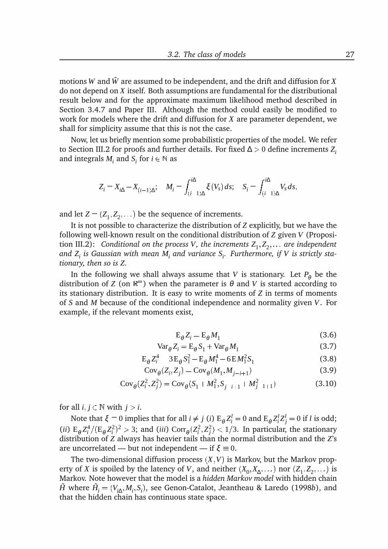
3.2. The class of models 27
motions W and W are assumed to be independent, and the drift and diffusion for Xdo not depend on X itself. Both assumptions are fundamental for the distributionalresult below and for the approximate maximum likelihood method described inSection 3.4.7 and Paper III. Although the method could easily be modified towork for models where the drift and diffusion for X are parameter dependent, weshall for simplicity assume that this is not the case.
Now, let us briefly mention some probabilistic properties of the model. We referto Section III.2 for proofs and further details. For fixed ∆ > 0 define increments Ziand integrals Mi and Si for i 2 N as
Zi = Xi∆X(i1)∆; Mi = Z i∆(i1)∆ ξ (Vs)ds; Si = Z i∆(i1)∆Vs ds;and let Z = (Z1;Z2; : : :) be the sequence of increments.
It is not possible to characterize the distribution of Z explicitly, but we have thefollowing well-known result on the conditional distribution of Z given V (Proposi-tion III.2): Conditional on the process V , the increments Z1;Z2; : : : are independent
and Zi is Gaussian with mean Mi and variance Si. Furthermore, if V is strictly sta-
tionary, then so is Z.
In the following we shall always assume that V is stationary. Let Pθ be thedistribution of Z (on R∞) when the parameter is θ and V is started according toits stationary distribution. It is easy to write moments of Z in terms of momentsof S and M because of the conditional independence and normality given V . Forexample, if the relevant moments exist,
Eθ Zi = Eθ M1 (3.6)
Varθ Zi = Eθ S1+Varθ M1 (3.7)
Eθ Z4i = 3Eθ S2
1+Eθ M41 +6EM2
1S1 (3.8)
Covθ (Zi;Z j) = Covθ (M1;M ji+1) (3.9)
Covθ (Z2i ;Z2
j ) = Covθ (S1+M21;S ji+1+M2
j1+1) (3.10)
for all i; j 2 N with j > i.
Note that ξ 0 implies that for all i 6= j (i) Eθ Zli = 0 and Eθ Zl
i Zlj = 0 if l is odd;
(ii) Eθ Z4i =(Eθ Z2
i )2 > 3; and (iii) Corrθ (Z2i ;Z2
j ) < 1=3. In particular, the stationarydistribution of Z always has heavier tails than the normal distribution and the Z’sare uncorrelated — but not independent — if ξ 0.
The two-dimensional diffusion process (X ;V) is Markov, but the Markov prop-erty of X is spoiled by the latency of V , and neither (X0;X∆; : : :) nor (Z1;Z2; : : :) isMarkov. Note however that the model is a hidden Markov model with hidden chainH where Hi = (Vi∆;Mi;Si), see Genon-Catalot, Jeantheau & Laredo (1998b), andthat the hidden chain has continuous state space.
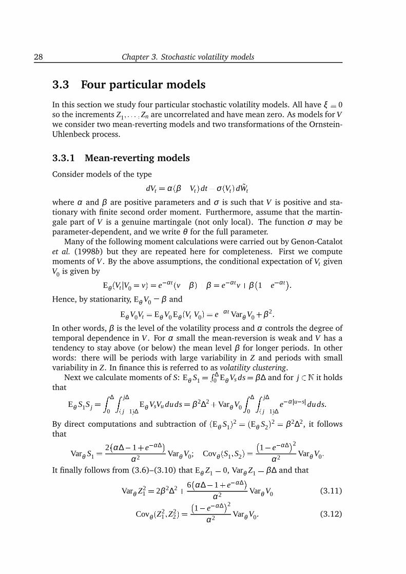
28 Chapter 3. Stochastic volatility models
3.3 Four particular models
In this section we study four particular stochastic volatility models. All have ξ 0so the increments Z1; : : : ;Zn are uncorrelated and have mean zero. As models for Vwe consider two mean-reverting models and two transformations of the Ornstein-Uhlenbeck process.
3.3.1 Mean-reverting models
Consider models of the type
dVt = α(β Vt)dt +σ(Vt)dWt
where α and β are positive parameters and σ is such that V is positive and sta-tionary with finite second order moment. Furthermore, assume that the martin-gale part of V is a genuine martingale (not only local). The function σ may beparameter-dependent, and we write θ for the full parameter.
Many of the following moment calculations were carried out by Genon-Catalotet al. (1998b) but they are repeated here for completeness. First we computemoments of V . By the above assumptions, the conditional expectation of Vt givenV0 is given by
Eθ (Vt jV0 = v) = eαt(vβ )+β = eαtv+β1 eαt:
Hence, by stationarity, Eθ V0 = β and
Eθ V0Vt = Eθ V0Eθ (Vt jV0) = eαt Varθ V0+β 2:In other words, β is the level of the volatility process and α controls the degree oftemporal dependence in V . For α small the mean-reversion is weak and V has atendency to stay above (or below) the mean level β for longer periods. In otherwords: there will be periods with large variability in Z and periods with smallvariability in Z. In finance this is referred to as volatility clustering.
Next we calculate moments of S: Eθ S1 = R ∆0 Eθ Vs ds = β∆ and for j 2 N it holds
that
Eθ S1S j = Z ∆
0
Z j∆( j1)∆ Eθ VsVu duds = β 2∆2+Varθ V0
Z ∆
0
Z j∆( j1)∆ eαjusj duds:By direct computations and subtraction of (Eθ S1)2 = (Eθ S2)2 = β 2∆2, it followsthat
Varθ S1 = 2α∆1+ eα∆
α2 Varθ V0; Covθ (S1;S2) = 1 eα∆2
α2 Varθ V0:It finally follows from (3.6)–(3.10) that Eθ Z1 = 0, Varθ Z1 = β∆ and that
Varθ Z21 = 2β 2∆2+ 6
α∆1+ eα∆
α2 Varθ V0 (3.11)
Covθ (Z21;Z2
2) = 1 eα∆2α2 Varθ V0: (3.12)
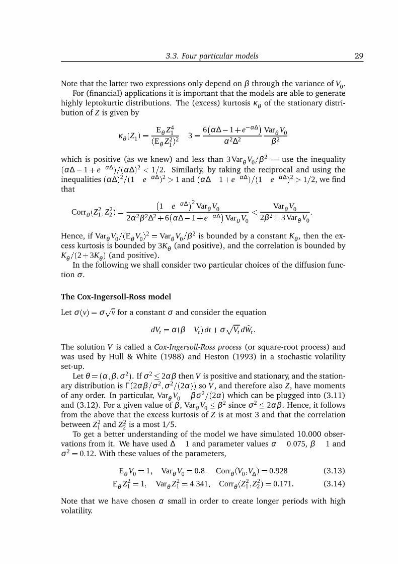
3.3. Four particular models 29
Note that the latter two expressions only depend on β through the variance of V0.For (financial) applications it is important that the models are able to generate
highly leptokurtic distributions. The (excess) kurtosis κθ of the stationary distri-bution of Z is given by
κθ (Z1) = Eθ Z41(Eθ Z21)2 3= 6
α∆1+ eα∆
α2∆2
Varθ V0
β 2
which is positive (as we knew) and less than 3Varθ V0=β 2 — use the inequality(α∆ 1+ eα∆)=(α∆)2 < 1=2. Similarly, by taking the reciprocal and using theinequalities (α∆)2=(1eα∆)2 > 1 and (α∆1+eα∆)=(1eα∆)2 > 1=2, we findthat
Corrθ (Z21;Z2
2) = 1 eα∆2Varθ V0
2α2β 2∆2+6α∆1+ eα∆
Varθ V0
< Varθ V0
2β 2+3Varθ V0:
Hence, if Varθ V0=(Eθ V0)2 = Varθ V0=β 2 is bounded by a constant Kθ , then the ex-cess kurtosis is bounded by 3Kθ (and positive), and the correlation is bounded byKθ=(2+3Kθ) (and positive).
In the following we shall consider two particular choices of the diffusion func-tion σ .
The Cox-Ingersoll-Ross model
Let σ(v) = σp
v for a constant σ and consider the equation
dVt = α(β Vt)dt +σp
Vt dWt :The solution V is called a Cox-Ingersoll-Ross process (or square-root process) andwas used by Hull & White (1988) and Heston (1993) in a stochastic volatilityset-up.
Let θ =(α;β ;σ2). If σ2 2αβ then V is positive and stationary, and the station-ary distribution is Γ(2αβ=σ2;σ2=(2α)) so V , and therefore also Z, have momentsof any order. In particular, Varθ V0 = βσ2=(2α) which can be plugged into (3.11)and (3.12). For a given value of β , Varθ V0 β 2 since σ2 2αβ . Hence, it followsfrom the above that the excess kurtosis of Z is at most 3 and that the correlationbetween Z2
1 and Z22 is a most 1/5.
To get a better understanding of the model we have simulated 10.000 obser-vations from it. We have used ∆ = 1 and parameter values α = 0:075, β = 1 andσ2 = 0:12. With these values of the parameters,
Eθ V0 = 1; Varθ V0 = 0:8; Corrθ (V0;V∆) = 0:928 (3.13)
Eθ Z21 = 1; Varθ Z2
1 = 4:341; Corrθ (Z21;Z2
2) = 0:171: (3.14)
Note that we have chosen α small in order to create longer periods with highvolatility.
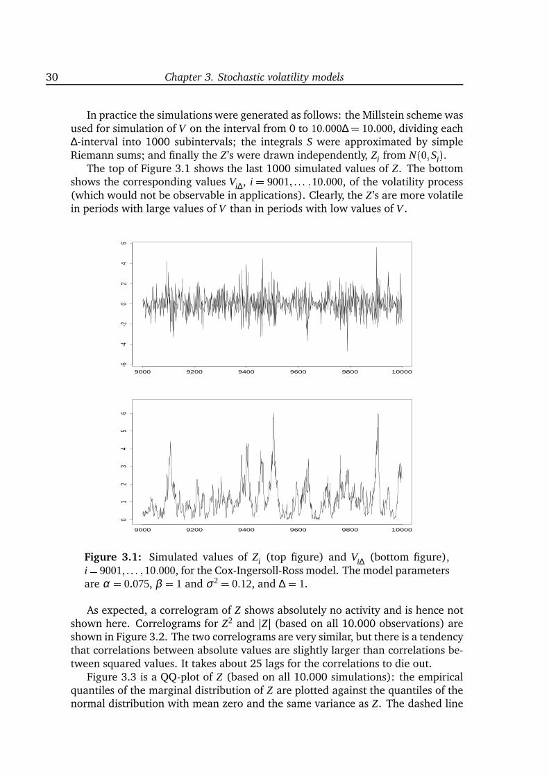
30 Chapter 3. Stochastic volatility models
In practice the simulations were generated as follows: the Millstein scheme wasused for simulation of V on the interval from 0 to 10:000∆ = 10:000, dividing each∆-interval into 1000 subintervals; the integrals S were approximated by simpleRiemann sums; and finally the Z’s were drawn independently, Zi from N(0;Si).
The top of Figure 3.1 shows the last 1000 simulated values of Z. The bottomshows the corresponding values Vi∆, i = 9001; : : : ;10:000, of the volatility process(which would not be observable in applications). Clearly, the Z’s are more volatilein periods with large values of V than in periods with low values of V .
9000 9200 9400 9600 9800 10000
-6-4
-20
24
6
9000 9200 9400 9600 9800 10000
01
23
45
6
Figure 3.1: Simulated values of Zi (top figure) and Vi∆ (bottom figure),i= 9001; : : : ;10:000, for the Cox-Ingersoll-Ross model. The model parametersare α = 0:075, β = 1 and σ2 = 0:12, and ∆ = 1.
As expected, a correlogram of Z shows absolutely no activity and is hence notshown here. Correlograms for Z2 and jZj (based on all 10.000 observations) areshown in Figure 3.2. The two correlograms are very similar, but there is a tendencythat correlations between absolute values are slightly larger than correlations be-tween squared values. It takes about 25 lags for the correlations to die out.
Figure 3.3 is a QQ-plot of Z (based on all 10.000 simulations): the empiricalquantiles of the marginal distribution of Z are plotted against the quantiles of thenormal distribution with mean zero and the same variance as Z. The dashed line
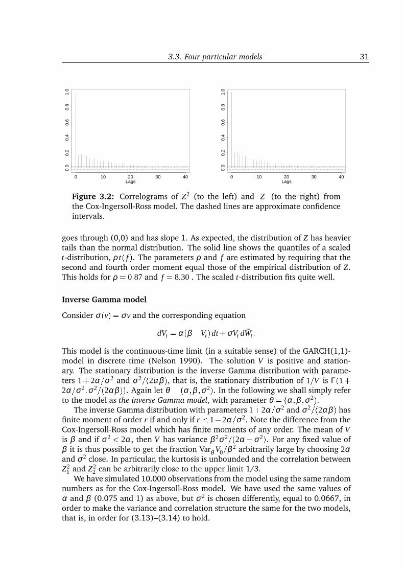
3.3. Four particular models 31
Lags0 10 20 30 40
0.0
0.2
0.4
0.6
0.8
1.0
Lags0 10 20 30 40
0.0
0.2
0.4
0.6
0.8
1.0
Figure 3.2: Correlograms of Z2 (to the left) and jZj (to the right) fromthe Cox-Ingersoll-Ross model. The dashed lines are approximate confidenceintervals.
goes through (0,0) and has slope 1. As expected, the distribution of Z has heaviertails than the normal distribution. The solid line shows the quantiles of a scaledt-distribution, ρ t( f ). The parameters ρ and f are estimated by requiring that thesecond and fourth order moment equal those of the empirical distribution of Z.This holds for ρ = 0:87 and f = 8:30 . The scaled t-distribution fits quite well.
Inverse Gamma model
Consider σ(v) = σv and the corresponding equation
dVt = α(β Vt)dt +σVt dWt :This model is the continuous-time limit (in a suitable sense) of the GARCH(1,1)-model in discrete time (Nelson 1990). The solution V is positive and station-ary. The stationary distribution is the inverse Gamma distribution with parame-ters 1+2α=σ2 and σ2=(2αβ ), that is, the stationary distribution of 1=V is Γ(1+2α=σ2;σ2=(2αβ )). Again let θ = (α;β ;σ2). In the following we shall simply referto the model as the inverse Gamma model, with parameter θ = (α;β ;σ2).
The inverse Gamma distribution with parameters 1+2α=σ2 and σ2=(2αβ ) hasfinite moment of order r if and only if r < 1+2α=σ2. Note the difference from theCox-Ingersoll-Ross model which has finite moments of any order. The mean of Vis β and if σ2 < 2α, then V has variance β 2σ2=(2α σ2). For any fixed value ofβ it is thus possible to get the fraction Varθ V0=β 2 arbitrarily large by choosing 2αand σ2 close. In particular, the kurtosis is unbounded and the correlation betweenZ2
1 and Z22 can be arbitrarily close to the upper limit 1/3.
We have simulated 10.000 observations from the model using the same randomnumbers as for the Cox-Ingersoll-Ross model. We have used the same values ofα and β (0.075 and 1) as above, but σ2 is chosen differently, equal to 0.0667, inorder to make the variance and correlation structure the same for the two models,that is, in order for (3.13)–(3.14) to hold.
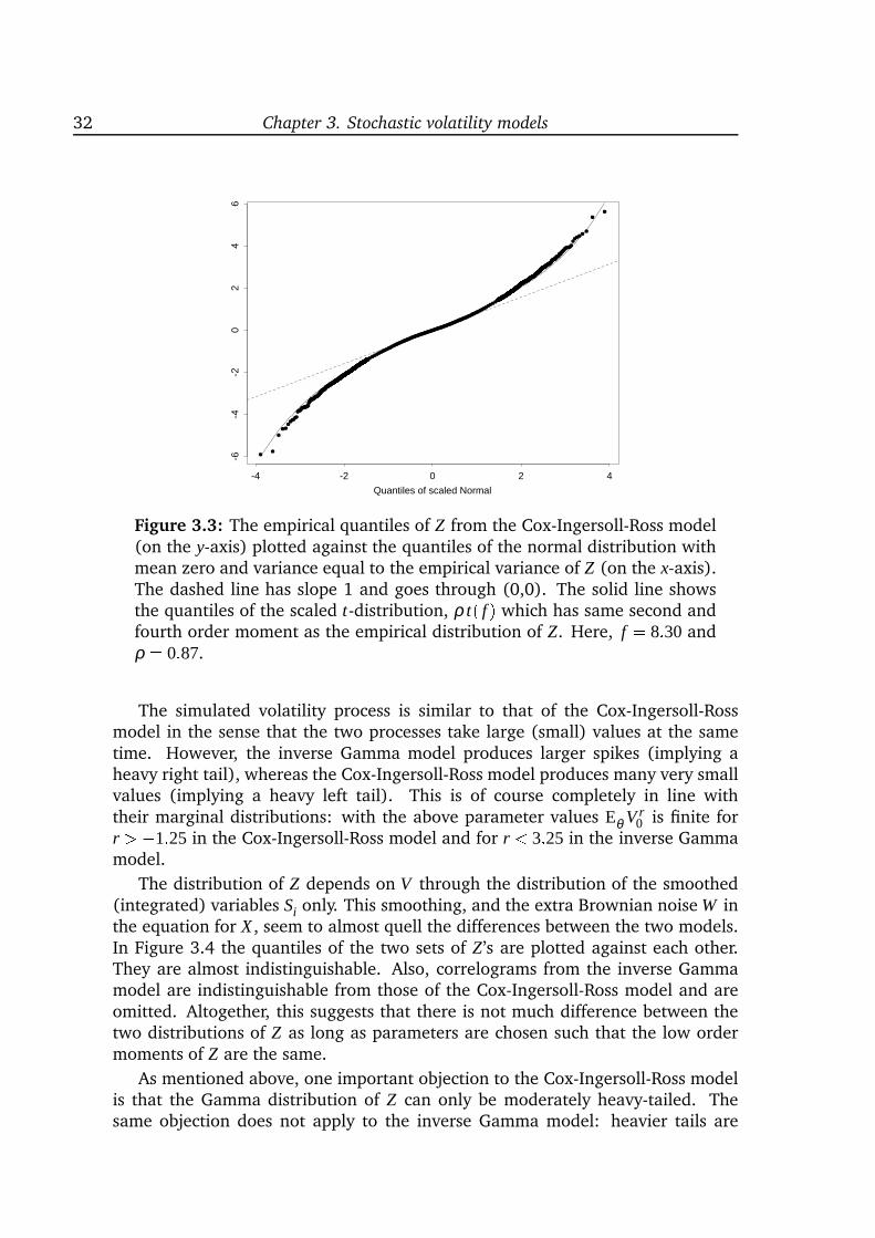
32 Chapter 3. Stochastic volatility models
Quantiles of scaled Normal
-4 -2 0 2 4
-6-4
-20
24
6
Figure 3.3: The empirical quantiles of Z from the Cox-Ingersoll-Ross model(on the y-axis) plotted against the quantiles of the normal distribution withmean zero and variance equal to the empirical variance of Z (on the x-axis).The dashed line has slope 1 and goes through (0,0). The solid line showsthe quantiles of the scaled t-distribution, ρ t( f ) which has same second andfourth order moment as the empirical distribution of Z. Here, f = 8:30 andρ = 0:87.
The simulated volatility process is similar to that of the Cox-Ingersoll-Rossmodel in the sense that the two processes take large (small) values at the sametime. However, the inverse Gamma model produces larger spikes (implying aheavy right tail), whereas the Cox-Ingersoll-Ross model produces many very smallvalues (implying a heavy left tail). This is of course completely in line withtheir marginal distributions: with the above parameter values Eθ V r
0 is finite forr > 1:25 in the Cox-Ingersoll-Ross model and for r < 3:25 in the inverse Gammamodel.
The distribution of Z depends on V through the distribution of the smoothed(integrated) variables Si only. This smoothing, and the extra Brownian noise W inthe equation for X , seem to almost quell the differences between the two models.In Figure 3.4 the quantiles of the two sets of Z’s are plotted against each other.They are almost indistinguishable. Also, correlograms from the inverse Gammamodel are indistinguishable from those of the Cox-Ingersoll-Ross model and areomitted. Altogether, this suggests that there is not much difference between thetwo distributions of Z as long as parameters are chosen such that the low ordermoments of Z are the same.
As mentioned above, one important objection to the Cox-Ingersoll-Ross modelis that the Gamma distribution of Z can only be moderately heavy-tailed. Thesame objection does not apply to the inverse Gamma model: heavier tails are
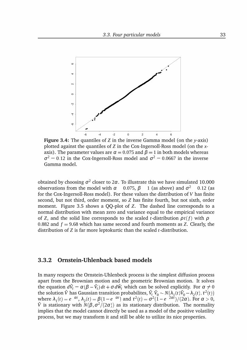
3.3. Four particular models 33
-6 -4 -2 0 2 4 6
-6-4
-20
24
6
Figure 3.4: The quantiles of Z in the inverse Gamma model (on the y-axis)plotted against the quantiles of Z in the Cox-Ingersoll-Ross model (on the x-axis). The parameter values are α = 0:075and β = 1 in both models whereasσ2 = 0:12 in the Cox-Ingersoll-Ross model and σ2 = 0:0667 in the inverseGamma model.
obtained by choosing σ2 closer to 2α. To illustrate this we have simulated 10.000observations from the model with α = 0:075, β = 1 (as above) and σ2 = 0:12 (asfor the Cox-Ingersoll-Ross model). For these values the distribution of V has finitesecond, but not third, order moment, so Z has finite fourth, but not sixth, ordermoment. Figure 3.5 shows a QQ-plot of Z. The dashed line corresponds to anormal distribution with mean zero and variance equal to the empirical varianceof Z, and the solid line corresponds to the scaled t-distribution ρ t( f ) with ρ =0:882and f = 9:68 which has same second and fourth moments as Z. Clearly, thedistribution of Z is far more leptokurtic than the scaled t-distribution.
3.3.2 Ornstein-Uhlenback based models
In many respects the Ornstein-Uhlenbeck process is the simplest diffusion processapart from the Brownian motion and the geometric Brownian motion. It solvesthe equation dVt = α(β Vt)dt +σ dWt which can be solved explicitly. For α 6= 0the solution V has Gaussian transition probabilites, Vt jV0 N(λ1(t)V0+λ2(t);τ2(t))where λ1(t) = eαt , λ2(t) = β (1 eαt) and τ2(t) = σ2(1 e2αt)=(2α). For α > 0,V is stationary with N(β ;σ2=(2α)) as its stationary distribution. The normalityimplies that the model cannot directly be used as a model of the positive volatilityprocess, but we may transform it and still be able to utilize its nice properties.
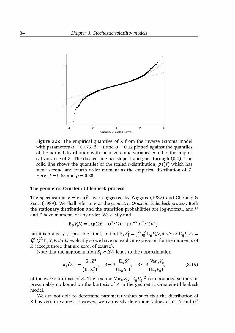
34 Chapter 3. Stochastic volatility models
Quantiles of scaled Normal
-4 -2 0 2 4
-50
5
Figure 3.5: The empirical quantiles of Z from the inverse Gamma modelwith parameters α = 0:075, β = 1 and σ = 0:12 plotted against the quantilesof the normal distribution with mean zero and variance equal to the empiri-cal variance of Z. The dashed line has slope 1 and goes through (0,0). Thesolid line shows the quantiles of the scaled t-distribution, ρ t( f ) which hassame second and fourth order moment as the empirical distribution of Z.Here, f = 9:68 and ρ = 0:88.
The geometric Ornstein-Uhlenbeck process
The specification V = exp(V ) was suggested by Wiggins (1987) and Chesney &Scott (1989). We shall refer to V as the geometric Ornstein-Uhlenbeck process. Boththe stationary distribution and the transition probabilities are log-normal, and Vand Z have moments of any order. We easily find
Eθ V0Vt = exp2β +σ2=(2α)+ eαtσ2=(2α);
but it is not easy (if possible at all) to find Eθ S21 = R ∆
0R ∆
0 Eθ VuVs duds or Eθ S1S2 =R ∆0R 2∆
∆ Eθ VuVs duds explicitly so we have no explicit expression for the moments ofZ (except those that are zero, of course).
Note that the approximation S1 ∆V0 leads to the approximation
κθ (Z1) = Eθ Z41
Eθ Z21
2 3= 3Eθ S2
1Eθ S1
2 3 3Varθ V0Eθ V0
2 (3.15)
of the excess kurtosis of Z. The fraction Varθ V0=(Eθ V0)2 is unbounded so there ispresumably no bound on the kurtosis of Z in the geometric Ornstein-Uhlenbeckmodel.
We are not able to determine parameter values such that the distribution ofZ has certain values. However, we can easily determine values of α, β and σ2
3.3. Four particular models 35
such that (3.13) holds: α = 0:0571, β = 0:294 and σ2 = 0:0672. Note that thevalue of σ2 is close to the corresponding value for the inverse Gamma model(0.0667). This is not very surprising since V , by Itô’s formula, solves the stochasticdifferential equation
dVt = αβ log(Vt)Vt +σ2Vt=2
dt +σVt dWt
with same diffusion function as the inverse Gamma model. Simulations of thegeometric Ornstein-Uhlenbeck process with the above parameters are almost in-distinguishable from those of the two mean-reverting models.
The squared Ornstein-Uhlenbeck process
The squared Ornstein-Uhlenbeck process V = V 2 was used by Scott (1987) and Stein& Stein (1991). Under this model, V and thus Z have moments of any order. It iseasily verified that Varθ V0=(Eθ V0)2 2 so the kurtosis of Z is presumably boundedby a value around 6, cf. (3.15). The model has several disadvantages comparedto the previous models: (i) V is not strictly positive but hits zero; (ii) V is nota diffusion unless β = 0 (the drift term in the stochastic differential equation forV cannot be written in terms of V but involves V as well); and (iii) there are noexplicit expressions for covariances between V0 and Vt , say.
The covariances may be calculated by simulation from the invariant distribu-tion of V , though. For this, note that Eθ V0Vt equals
τ2(t)+λ 22(t)Eθ V0+λ 2
1 (t)Eθ V 20 +2λ1(t)λ2(t)Eθ
V 3=2
0gV0;β ;σ2=(2α)
where the function g is given by
g(v;m;s2) = exp(mpv=s2)exp(mp
v=s2)exp(mpv=s2)+exp(m
pv=s2) :
The formula is derived via repeated expectations
EθVt jV0
= EθV 2
t jV 20
= Eθ
EθV 2
t
V0
V 20
;where the inner expectation is computable as the transitions of V are normal.
For α = 0:0661, β = 0:880 and σ2 = 0:0298 the values of Eθ V0, Varθ V0 andCorrθ (V0;V∆) are (roughly) as in (3.13). Simulations of Z from the model withthese parameter values are very similar to the simulations of the three previousmodels.
3.3.3 Concluding remarks
The above investigation indicates that the four models produce very similar dis-tributions of Z — as long as the model parameters are chosen such that the low-order moments of V are the same. The fact that the eighth order moment of Z
36 Chapter 3. Stochastic volatility models
is infinite for the inverse Gamma model and finite for the other models is hardlyrecognizable from the simulations. The reason is that differences in the volatil-ity distributions are suppressed by smoothing (when V is transformed to integralsS) and by the extra noise in the equation for X . Still, there are important dif-ferences between the four models in their ability to create strong leptokurtosisand large auto-correlations: only two models (the inverse Gamma and the geo-metric Ornstein-Uhlenbeck) allow for arbitrarily large kurtosis and maximal auto-correlation (which is 1/3).
Of course one could think of many other models for the volatility process. Pre-sumably, most of them would generate distributions of Z very similar to thoseabove as long as parameters are chosen appropriately. In conclusion: If dataare heavy-tailed to an extent that cannot be modeled by the two restrictive mod-els, then one should use the inverse Gamma model or the geometric Ornstein-Uhlenbeck model. On the other hand, if there are no stylized facts contradictingany of the models and if there are no prior (economic) reasons to prefer onespecification to another, then it seems less important which one of the modelsis applied. Note however that the squared Ornstein-Uhlenbeck model has somedisadvantages which makes it the least attractive of the four models.
3.4 Estimation methods
In the majority of the early finance papers on stochastic volatility models (refer-enced in Section 3.3) no or little attention is paid to estimation problems. Thepossibility of doing parameter estimation via historical option prices and reversedversions of the option pricing formulas is mentioned but not carried out in prac-tice. Anyway, this is a relatively indirect estimation approach. Only Scott (1987)and Chesney & Scott (1989) address the estimation problem seriously and derivemoment-like estimators based on historical stock prices.
Recently there has been some progress in the statistics literature concerningstochastic volatility models, and the aim of this section is to give an overview ofexisting methods. Furthermore, a new method based on simulated approximationsto the likelihood is reviewed in Section 3.4.7; a detailed discussion is provided inPaper III. There exist review papers on statistical analysis of stochastic volatilitymodels defined in discrete time (Ghysels et al. 1996, Shephard 1996), but as men-tioned in the beginning of this chapter the continuous-time models are in generalmore difficult to handle.
Now, the situation is the following. Consider the model given by (3.4)–(3.5),and assume that observations X0;X∆; : : : ;Xn∆ of X are available for some fixed ∆while the volatility process is unobserved. Because of the nice conditional distri-bution (given V ) of the increments Zi = Xi∆X(i1)∆, i = 1; : : : ;n, it is natural to
base estimation on the increments. The estimation problem is inherently difficult:apart from the usual problems due to discrete-time observations of a continuous-time system, we are faced with yet another missing data problem due to the la-tency of V . As a consequence, most of the estimation procedures below are very
3.4. Estimation methods 37
computationally intensive.Some remarks before reviewing the methods. First note that exact maximum
likelihood estimation is not really an option: For an observation (z1; : : : ;zn) it fol-lows by conditional independence and normality given V that the likelihood func-tion is given by
Ln(θ) = Z n
∏i=1
1p2πsi
exp(zimi)2
2si
dπn
θ (hn) = Eπnθ
n
∏i=1
ϕ(zi;Mi;Si) (3.16)
where we have used the notation ϕ(;m;s) for the density of N(m;s) and πnθ for
the distribution of Hn = ((M1;S1); : : : ;(Mn;Sn)). There is no closed-form expressionfor the likelihood, not even for very simple models of V . In principle, values ofthe likelihood function could be computed by simulation as follows: (i) simulatea large number of paths V up to time n∆ according to (3.5); (ii) calculate foreach simulation (an approximation to) the integrals Mi and Si, i = 1; : : : ;n, andthe above product; and (iii) calculate the average of the simulated product values.However, this is not feasible in practice as a huge number of simulations wouldbe required in order for the average to converge, that is, in order to compute thelikelihood for just a single value of the parameter. Our approach in Section 3.4.7and Paper III will be to use the simulation approach on approximations to thelikelihood function.
Second, as we are faced with discrete-time observations of a continuous-timemodel, a natural approach would be to perform estimation in a discrete-time ap-proximation to the original model. If we use the Euler scheme or some stochas-tic volatility model in discrete time, we are still left with an unobserved compo-nent which makes estimation difficult. However, Nelson (1990) showed that somediffusion processes can be approximated by ARCH type processes. For example,the limit of a GARCH(1,1) model is the stochastic volatility model with inverseGamma-distributed volatility discussed in Section 3.3.1. Approximation by ARCHtype models is advantageous as estimation is relatively simple. The problem is ofcourse that the approximation is only good if the time between observations, ∆, issmall so consistent estimators are obtained only if ∆ ! 0. The methods based onauxiliary models (Section 3.4.5) correct for this bias by simulation.
Third, apart from estimation of the model parameters, one could also be inter-ested in filtering, that is, estimation of the unobserved volatility process V . Nelson(1992) suggests a filtering method based on ARCH approximations. Given esti-mates, V0;V∆; : : : ;Vn, one could estimate θ by one of the methods in Chapter 2as if V0;V∆; : : : ;Vn∆ were actual observations of V . Nielsen, Vestergaard & Madsen(2000) use another technique that simultaneously delivers parameter estimatesand estimates of the volatility process.
Except from Section 3.4.6 where the latter filter method is reviewed, the rest ofthis chapter is exclusively about parameter estimation. We discuss simple momentestimators in Section 3.4.1, estimation based on a simple approximation to themarginal distribution in Section 3.4.2, prediction-based estimating functions inSection 3.4.3, Bayesian analysis in Section 3.4.4, and methods based on auxiliary
38 Chapter 3. Stochastic volatility models
models in Section 3.4.5. The latter two sections are very brief as the methodshave been discussed in Sections 2.5 and 2.6 for pure diffusion models. The newsimulated, approximate maximum likelihood method is discussed in Section 3.4.7(and Paper III). Conclusions are drawn in Section 3.4.8.
3.4.1 Moment estimation
Moment estimators are obtained by matching empirical and theoretical moments.As already noted, moments of Z are easily expressed in terms of moments of theintegrals M and S. These can be calculated explicitly in simple mean-revertingmodels (Section 3.3.1) and by simulation in more complex models.
Recall that p is the dimension of the parameter and choose p functionalsg1; : : : ;gp, for example of type z1! z j
1and (z1;z2)! z j
1z j2
for suitable (small) valuesof j. The parameter should be uniquely determined by the theoretical moments ofg1; : : : ;gp. With sloppy notation, the requirement is
Eθ g1; : : : ;Eθ gp 6= Eθ 0 g1; : : : ;Eθ 0 gp
; θ 6= θ 0:Then a natural estimate of θ is the value that makes the theoretical momentsof g1; : : : ;gp match their empirical counterparts. Also, moments may be used asbuilding blocks for the generalized method of moments, GMM (Hansen 1982) whichis very popular in the econometric literature. Here q > p moment functionals areselected, and θ is estimated such that certain linear combinations of the theoreticalmoments are close to their empirical counterparts.
Genon-Catalot et al. (1998b) showed consistency and asymptotic normality ofthe empirical moments (in the model with ξ 0). By transformation, the proper-ties carry over to the moment estimators. Moment matching is quick compared toother methods, in particular for models where moments are known analytically.However, a simulation study in Section III.7 indicates that a solution to the esti-mating equation fairly often does not exist and that moments estimators can bevery poor for a sample size of 500.
3.4.2 Approximation of the marginal density
In Section 3.4.7 we study approximations to the likelihood. The simplest of theseapproximations, denoted L0
n, corresponds to pretending that Z1; : : : ;Zn are inde-pendent, identically distributed according to the stationary (marginal) distribu-tion, that is L0
n(θ) = ∏ni=1 p1
θ (zi) where
p1θ (z) = Z
ϕ(z;m;s)dπ1θ(m;s) = Eπ1
θϕ(z;M;S)
is the stationary density of Z and π1θ is the distribution of (M1;S1).
The distribution of (M1;S1) is not known so we have no explicit expressionfor the above density. In Section 3.4.7 we suggest to determine it by simulation.
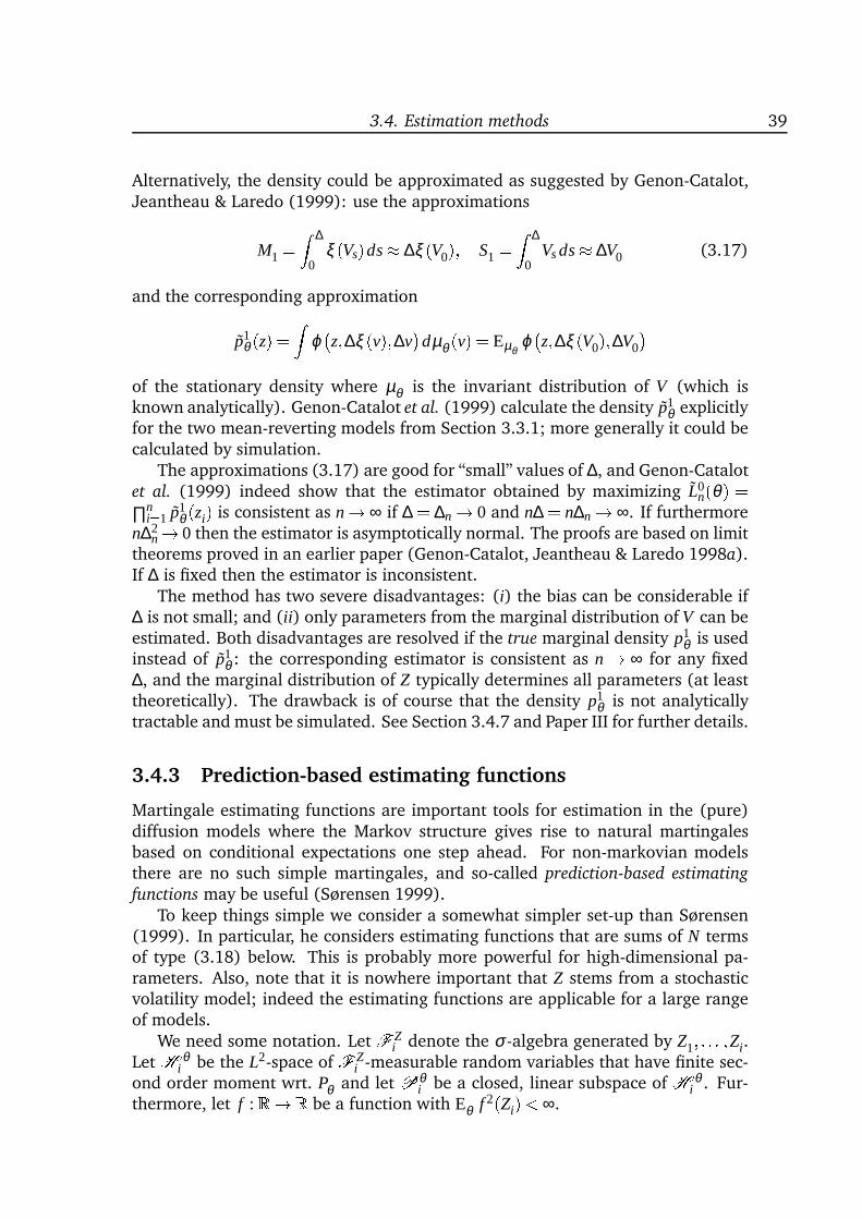
3.4. Estimation methods 39
Alternatively, the density could be approximated as suggested by Genon-Catalot,Jeantheau & Laredo (1999): use the approximations
M1 = Z ∆
0ξ (Vs)ds ∆ξ (V0); S1 = Z ∆
0Vs ds ∆V0 (3.17)
and the corresponding approximation
p1θ (z) = Z
ϕz;∆ξ (v);∆v
dµθ (v) = Eµθ
ϕz;∆ξ (V0);∆V0
of the stationary density where µθ is the invariant distribution of V (which isknown analytically). Genon-Catalot et al. (1999) calculate the density p1
θ explicitlyfor the two mean-reverting models from Section 3.3.1; more generally it could becalculated by simulation.
The approximations (3.17) are good for “small” values of ∆, and Genon-Catalotet al. (1999) indeed show that the estimator obtained by maximizing L0
n(θ) =∏n
i=1 p1θ (zi) is consistent as n! ∞ if ∆ = ∆n ! 0 and n∆ = n∆n ! ∞. If furthermore
n∆2n ! 0 then the estimator is asymptotically normal. The proofs are based on limit
theorems proved in an earlier paper (Genon-Catalot, Jeantheau & Laredo 1998a).If ∆ is fixed then the estimator is inconsistent.
The method has two severe disadvantages: (i) the bias can be considerable if∆ is not small; and (ii) only parameters from the marginal distribution of V can beestimated. Both disadvantages are resolved if the true marginal density p1
θ is usedinstead of p1
θ : the corresponding estimator is consistent as n ! ∞ for any fixed∆, and the marginal distribution of Z typically determines all parameters (at leasttheoretically). The drawback is of course that the density p1
θ is not analyticallytractable and must be simulated. See Section 3.4.7 and Paper III for further details.
3.4.3 Prediction-based estimating functions
Martingale estimating functions are important tools for estimation in the (pure)diffusion models where the Markov structure gives rise to natural martingalesbased on conditional expectations one step ahead. For non-markovian modelsthere are no such simple martingales, and so-called prediction-based estimating
functions may be useful (Sørensen 1999).To keep things simple we consider a somewhat simpler set-up than Sørensen
(1999). In particular, he considers estimating functions that are sums of N termsof type (3.18) below. This is probably more powerful for high-dimensional pa-rameters. Also, note that it is nowhere important that Z stems from a stochasticvolatility model; indeed the estimating functions are applicable for a large rangeof models.
We need some notation. Let F Zi denote the σ -algebra generated by Z1; : : : ;Zi.
Let H θi be the L2-space of F Z
i -measurable random variables that have finite sec-ond order moment wrt. Pθ and let Pθ
i be a closed, linear subspace of H θi . Fur-
thermore, let f : R ! R be a function with Eθ f 2(Zi)< ∞.
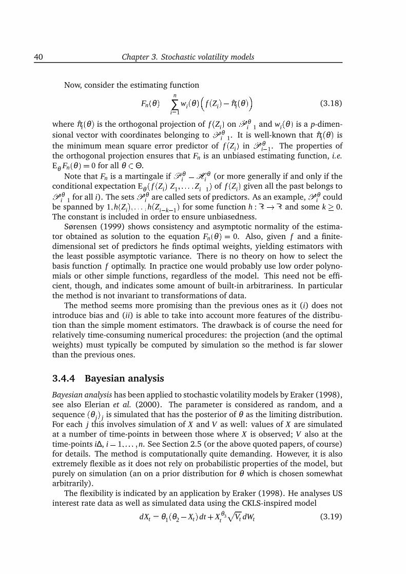
40 Chapter 3. Stochastic volatility models
Now, consider the estimating function
Fn(θ) = n
∑i=1
wi(θ) f (Zi) πi(θ) (3.18)
where πi(θ) is the orthogonal projection of f (Zi) on Pθi1 and wi(θ) is a p-dimen-
sional vector with coordinates belonging to Pθi1. It is well-known that πi(θ) is
the minimum mean square error predictor of f (Zi) in Pθi1. The properties of
the orthogonal projection ensures that Fn is an unbiased estimating function, i.e.
Eθ Fn(θ) = 0 for all θ 2 Θ.
Note that Fn is a martingale if Pθi =H θ
i (or more generally if and only if theconditional expectation Eθ ( f (Zi)jZ1; : : : ;Zi1) of f (Zi) given all the past belongs toPθ
i1 for all i). The setsPθi are called sets of predictors. As an example,Pθ
i couldbe spanned by 1;h(Zi); : : : ;h(Zik+1) for some function h : R ! R and some k 0.The constant is included in order to ensure unbiasedness.
Sørensen (1999) shows consistency and asymptotic normality of the estima-tor obtained as solution to the equation Fn(θ) = 0. Also, given f and a finite-dimensional set of predictors he finds optimal weights, yielding estimators withthe least possible asymptotic variance. There is no theory on how to select thebasis function f optimally. In practice one would probably use low order polyno-mials or other simple functions, regardless of the model. This need not be effi-cient, though, and indicates some amount of built-in arbitrariness. In particularthe method is not invariant to transformations of data.
The method seems more promising than the previous ones as it (i) does notintroduce bias and (ii) is able to take into account more features of the distribu-tion than the simple moment estimators. The drawback is of course the need forrelatively time-consuming numerical procedures: the projection (and the optimalweights) must typically be computed by simulation so the method is far slowerthan the previous ones.
3.4.4 Bayesian analysis
Bayesian analysis has been applied to stochastic volatility models by Eraker (1998),see also Elerian et al. (2000). The parameter is considered as random, and asequence (θ j) j is simulated that has the posterior of θ as the limiting distribution.For each j this involves simulation of X and V as well: values of X are simulatedat a number of time-points in between those where X is observed; V also at thetime-points i∆, i = 1; : : : ;n. See Section 2.5 (or the above quoted papers, of course)for details. The method is computationally quite demanding. However, it is alsoextremely flexible as it does not rely on probabilistic properties of the model, butpurely on simulation (an on a prior distribution for θ which is chosen somewhatarbitrarily).
The flexibility is indicated by an application by Eraker (1998). He analyses USinterest rate data as well as simulated data using the CKLS-inspired model
dXt = θ1(θ2Xt)dt +Xθ3t
pVt dWt (3.19)
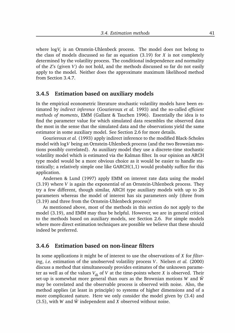
3.4. Estimation methods 41
where logVt is an Ornstein-Uhlenbeck process. The model does not belong tothe class of models discussed so far as equation (3.19) for X is not completelydetermined by the volatility process. The conditional independence and normalityof the Z’s (given V ) do not hold, and the methods discussed so far do not easilyapply to the model. Neither does the approximate maximum likelihood methodfrom Section 3.4.7.
3.4.5 Estimation based on auxiliary models
In the empirical econometric literature stochastic volatility models have been es-timated by indirect inference (Gourieroux et al. 1993) and the so-called efficient
methods of moments, EMM (Gallant & Tauchen 1996). Essentially the idea is tofind the parameter value for which simulated data resembles the observed datathe most in the sense that the simulated data and the observations yield the sameestimator in some auxiliary model. See Section 2.6 for more details.
Gourieroux et al. (1993) apply indirect inference to the modified Black-Scholesmodel with logV being an Ornstein-Uhlenbeck process (and the two Brownian mo-tions possibly correlated). As auxiliary model they use a discrete-time stochasticvolatility model which is estimated via the Kalman filter. In our opinion an ARCHtype model would be a more obvious choice as it would be easier to handle sta-tistically; a relatively simple one like GARCH(1,1) would probably suffice for thisapplication.
Andersen & Lund (1997) apply EMM on interest rate data using the model(3.19) where V is again the exponential of an Ornstein-Uhlenbeck process. Theytry a few different, though similar, ARCH type auxiliary models with up to 26parameters whereas the model of interest has six parameters only (three from(3.19) and three from the Ornstein-Uhlenbeck process)!
As mentioned above, most of the methods in this section do not apply to themodel (3.19), and EMM may thus be helpful. However, we are in general criticalto the methods based on auxiliary models, see Section 2.6. For simple modelswhere more direct estimation techniques are possible we believe that these shouldindeed be preferred.
3.4.6 Estimation based on non-linear filters
In some applications it might be of interest to use the observations of X for filter-
ing, i.e. estimation of the unobserved volatility process V . Nielsen et al. (2000)discuss a method that simultaneously provides estimates of the unknown parame-ter as well as of the values Vi∆ of V at the time-points where X is observed. Theirset-up is somewhat more general than ours as the Brownian motions W and Wmay be correlated and the observable process is observed with noise. Also, themethod applies (at least in principle) to systems of higher dimensions and of amore complicated nature. Here we only consider the model given by (3.4) and(3.5), with W and W independent and X observed without noise.
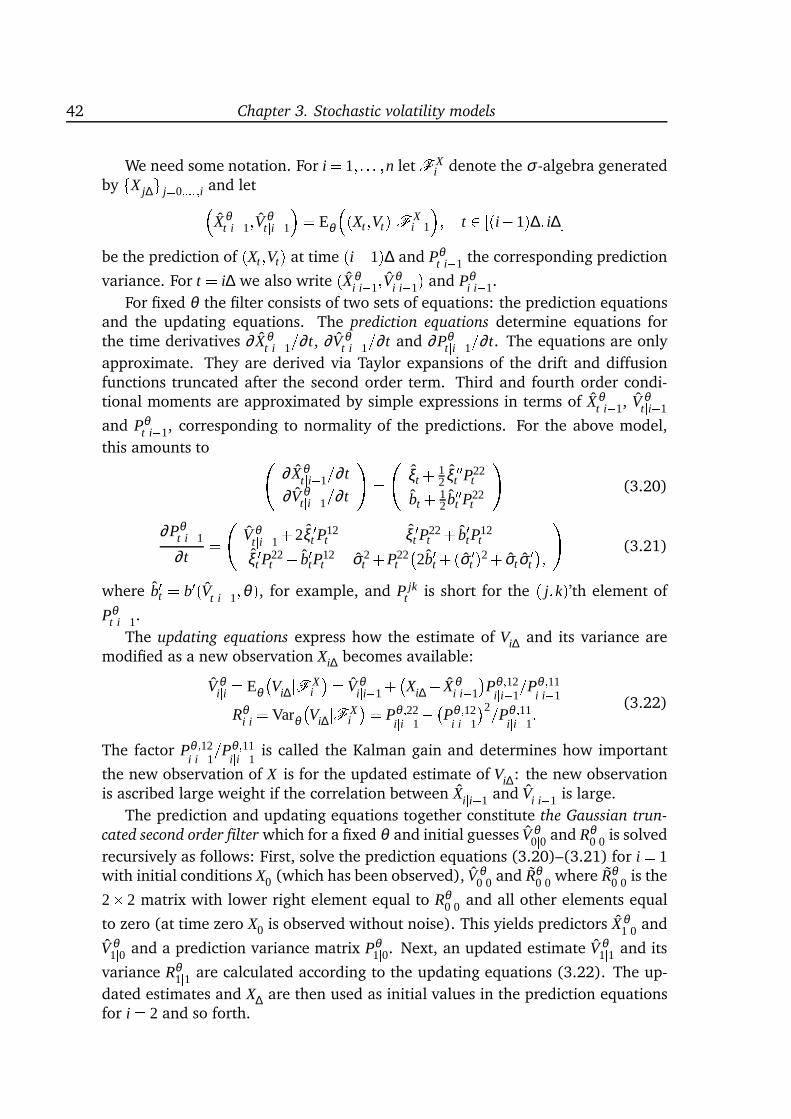
42 Chapter 3. Stochastic volatility models
We need some notation. For i = 1; : : : ;n letF Xi denote the σ -algebra generated
by fX j∆g j=0;::: ;i and letXθ
tji1;V θtji1
= Eθ
(Xt;Vt)F Xi1
; t 2 [(i1)∆; i∆be the prediction of (Xt;Vt) at time (i1)∆ and Pθ
tji1 the corresponding prediction
variance. For t = i∆ we also write (Xθiji1;V θ
iji1) and Pθiji1.
For fixed θ the filter consists of two sets of equations: the prediction equationsand the updating equations. The prediction equations determine equations forthe time derivatives ∂ Xθ
tji1=∂ t, ∂V θtji1=∂ t and ∂Pθ
tji1=∂ t. The equations are only
approximate. They are derived via Taylor expansions of the drift and diffusionfunctions truncated after the second order term. Third and fourth order condi-tional moments are approximated by simple expressions in terms of Xθ
tji1, V θtji1
and Pθtji1, corresponding to normality of the predictions. For the above model,
this amounts to ∂ Xθ
tji1=∂ t
∂V θtji1=∂ t
!= ξt + 12ξ 00t P22
t
bt + 12b00t P22
t
!(3.20)
∂Pθtji1
∂ t= V θ
tji1+2ξ 0t P12t ξ 0t P22
t + b0tP12t
ξ 0t P22t + b0tP12
t σ2t +P22
t
2b0t +(σ 0
t )2+ σt σ 0t
; ! (3.21)
where b0t = b0(Vtji1;θ), for example, and P jkt is short for the ( j;k)’th element of
Pθtji1.
The updating equations express how the estimate of Vi∆ and its variance aremodified as a new observation Xi∆ becomes available:
V θiji = Eθ
Vi∆jF X
i
= V θiji1+ Xi∆ Xθ
iji1
Pθ ;12
iji1=Pθ ;11
iji1
Rθiji = Varθ
Vi∆jF X
i
= Pθ ;22iji1
Pθ ;12iji1
2=Pθ ;11iji1
: (3.22)
The factor Pθ ;12iji1
=Pθ ;11iji1
is called the Kalman gain and determines how important
the new observation of X is for the updated estimate of Vi∆: the new observationis ascribed large weight if the correlation between Xiji1 and Viji1 is large.
The prediction and updating equations together constitute the Gaussian trun-
cated second order filter which for a fixed θ and initial guesses V θ0j0 and Rθ
0j0 is solved
recursively as follows: First, solve the prediction equations (3.20)–(3.21) for i = 1with initial conditions X0 (which has been observed), V θ
0j0 and Rθ0j0 where Rθ
0j0 is the
22 matrix with lower right element equal to Rθ0j0 and all other elements equal
to zero (at time zero X0 is observed without noise). This yields predictors Xθ1j0 and
V θ1j0 and a prediction variance matrix Pθ
1j0. Next, an updated estimate V θ1j1 and its
variance Rθ1j1 are calculated according to the updating equations (3.22). The up-
dated estimates and X∆ are then used as initial values in the prediction equationsfor i = 2 and so forth.
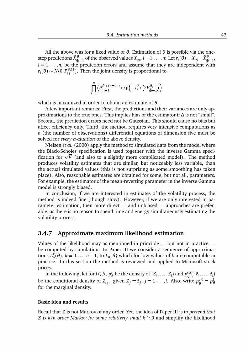
3.4. Estimation methods 43
All the above was for a fixed value of θ . Estimation of θ is possible via the one-step predictions Xθ
iji1 of the observed values Xi∆, i= 1; : : : ;n: Let ri(θ)=Xi∆Xθiji1,
i = 1; : : : ;n, be the prediction errors and assume that they are independent withri(θ) N(0;Pθ ;11
iji1). Then the joint density is proportional to
n
∏i=1
Pθ ;11
iji1
1=2expr2
i =2Pθ ;11iji1
which is maximized in order to obtain an estimate of θ .
A few important remarks: First, the predictions and their variances are only ap-proximations to the true ones. This implies bias of the estimator if ∆ is not “small”.Second, the prediction errors need not be Gaussian. This should cause no bias butaffect efficiency only. Third, the method requires very intensive computations asn (the number of observations) differential equations of dimension five must besolved for every evaluation of the above density.
Nielsen et al. (2000) apply the method to simulated data from the model wherethe Black-Scholes specification is used together with the inverse Gamma speci-fication for
pV (and also to a slightly more complicated model). The method
produces volatility estimates that are similar, but noticeably less variable, thanthe actual simulated values (this is not surprising as some smoothing has takenplace). Also, reasonable estimates are obtained for some, but not all, parameters.For example, the estimator of the mean-reverting parameter in the inverse Gammamodel is strongly biased.
In conclusion, if we are interested in estimates of the volatility process, themethod is indeed fine (though slow). However, if we are only interested in pa-rameter estimation, then more direct — and unbiased — approaches are prefer-able, as there is no reason to spend time and energy simultaneously estimating thevolatility process.
3.4.7 Approximate maximum likelihood estimation
Values of the likelihood may as mentioned in principle — but not in practice —be computed by simulation. In Paper III we consider a sequence of approxima-tions Lk
n(θ), k = 0; : : : ;n1, to Ln(θ) which for low values of k are computable inpractice. In this section the method is reviewed and applied to Microsoft stockprices.
In the following, let for i2N , piθ be the density of (Z1; : : : ;Zi) and pc;i
θ (jz1; : : : ; zi)be the conditional density of Zi+1 given Z j = z j, j = 1; : : : ; i. Also, write pc;0
θ = p1θ
for the marginal density.
Basic idea and results
Recall that Z is not Markov of any order. Yet, the idea of Paper III is to pretend that
Z is k’th order Markov for some relatively small k 0 and simplify the likelihood
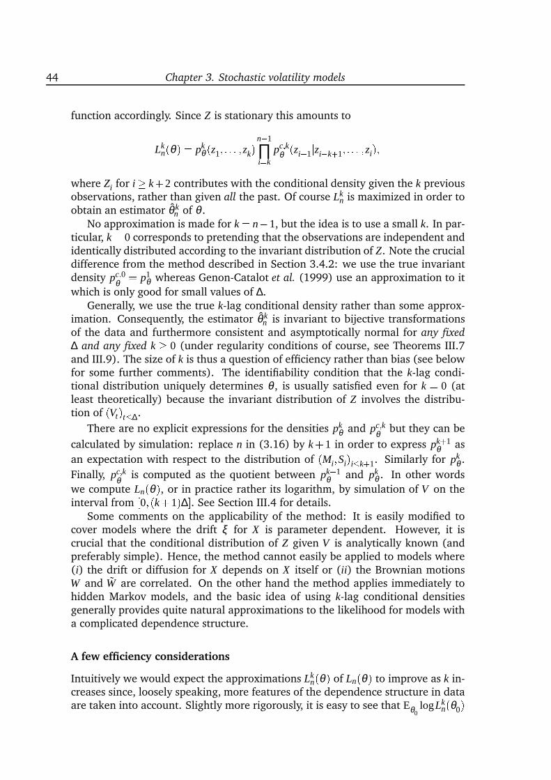
44 Chapter 3. Stochastic volatility models
function accordingly. Since Z is stationary this amounts to
Lkn(θ) = pk
θ (z1; : : : ;zk)n1
∏i=k
pc;kθ (zi+1jzik+1; : : : ;zi);
where Zi for i k+2 contributes with the conditional density given the k previousobservations, rather than given all the past. Of course Lk
n is maximized in order toobtain an estimator θ k
n of θ .No approximation is made for k = n1, but the idea is to use a small k. In par-
ticular, k = 0 corresponds to pretending that the observations are independent andidentically distributed according to the invariant distribution of Z. Note the crucialdifference from the method described in Section 3.4.2: we use the true invariantdensity pc;0
θ = p1θ whereas Genon-Catalot et al. (1999) use an approximation to it
which is only good for small values of ∆.Generally, we use the true k-lag conditional density rather than some approx-
imation. Consequently, the estimator θ kn is invariant to bijective transformations
of the data and furthermore consistent and asymptotically normal for any fixed
∆ and any fixed k 0 (under regularity conditions of course, see Theorems III.7and III.9). The size of k is thus a question of efficiency rather than bias (see belowfor some further comments). The identifiability condition that the k-lag condi-tional distribution uniquely determines θ , is usually satisfied even for k = 0 (atleast theoretically) because the invariant distribution of Z involves the distribu-tion of (Vt)t∆.
There are no explicit expressions for the densities pkθ and pc;k
θ but they can be
calculated by simulation: replace n in (3.16) by k+1 in order to express pk+1θ as
an expectation with respect to the distribution of (Mi;Si)ik+1. Similarly for pkθ .
Finally, pc;kθ is computed as the quotient between pk+1
θ and pkθ . In other words
we compute Ln(θ), or in practice rather its logarithm, by simulation of V on theinterval from [0;(k+1)∆. See Section III.4 for details.
Some comments on the applicability of the method: It is easily modified tocover models where the drift ξ for X is parameter dependent. However, it iscrucial that the conditional distribution of Z given V is analytically known (andpreferably simple). Hence, the method cannot easily be applied to models where(i) the drift or diffusion for X depends on X itself or (ii) the Brownian motionsW and W are correlated. On the other hand the method applies immediately tohidden Markov models, and the basic idea of using k-lag conditional densitiesgenerally provides quite natural approximations to the likelihood for models witha complicated dependence structure.
A few efficiency considerations
Intuitively we would expect the approximations Lkn(θ) of Ln(θ) to improve as k in-
creases since, loosely speaking, more features of the dependence structure in dataare taken into account. Slightly more rigorously, it is easy to see that Eθ0
logLkn(θ0)
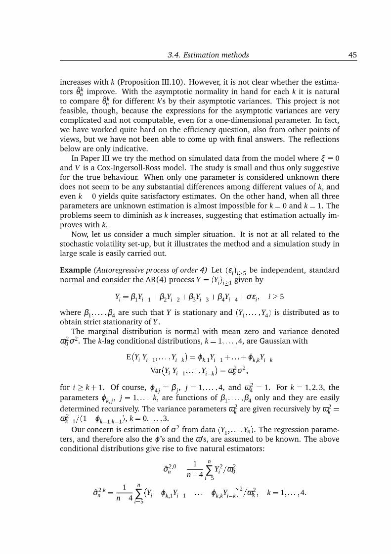
3.4. Estimation methods 45
increases with k (Proposition III.10). However, it is not clear whether the estima-tors θ k
n improve. With the asymptotic normality in hand for each k it is naturalto compare θ k
n for different k’s by their asymptotic variances. This project is notfeasible, though, because the expressions for the asymptotic variances are verycomplicated and not computable, even for a one-dimensional parameter. In fact,we have worked quite hard on the efficiency question, also from other points ofviews, but we have not been able to come up with final answers. The reflectionsbelow are only indicative.
In Paper III we try the method on simulated data from the model where ξ 0and V is a Cox-Ingersoll-Ross model. The study is small and thus only suggestivefor the true behaviour. When only one parameter is considered unknown theredoes not seem to be any substantial differences among different values of k, andeven k = 0 yields quite satisfactory estimates. On the other hand, when all threeparameters are unknown estimation is almost impossible for k = 0 and k = 1. Theproblems seem to diminish as k increases, suggesting that estimation actually im-proves with k.
Now, let us consider a much simpler situation. It is not at all related to thestochastic volatility set-up, but it illustrates the method and a simulation study inlarge scale is easily carried out.
Example (Autoregressive process of order 4) Let (εi)i5 be independent, standardnormal and consider the AR(4) process Y = (Yi)i1 given by
Yi = β1Yi1+β2Yi2+β3Yi3+β4Yi4+σεi; i 5
where β1; : : : ;β4 are such that Y is stationary and (Y1; : : : ;Y4) is distributed as toobtain strict stationarity of Y .
The marginal distribution is normal with mean zero and variance denotedω2
0σ2. The k-lag conditional distributions, k = 1; : : : ;4, are Gaussian with
EYijYi1; : : : ;Yik
= ϕk;1Yi1+ : : :+ϕk;kYik
VarYijYi1; : : : ;Yik
= ω2k σ2;
for i k + 1. Of course, ϕ4 j = β j, j = 1; : : : ;4, and ω24 = 1. For k = 1;2;3, the
parameters ϕk; j, j = 1; : : : ;k, are functions of β1; : : : ;β4 only and they are easily
determined recursively. The variance parameters ω2k are given recursively by ω2
k =ω2
k+1=(1ϕk+1;k+1), k = 0; : : : ;3.
Our concern is estimation of σ2 from data (Y1; : : : ;Yn). The regression parame-ters, and therefore also the ϕ ’s and the ω ’s, are assumed to be known. The aboveconditional distributions give rise to five natural estimators:
σ2;0n = 1
n4
n
∑i=5
Y 2i =ω2
0
σ2;kn = 1
n4
n
∑i=5
Yiϕk;1Yi1 : : :ϕk;kYik
2=ω2k ; k = 1; : : : ;4:
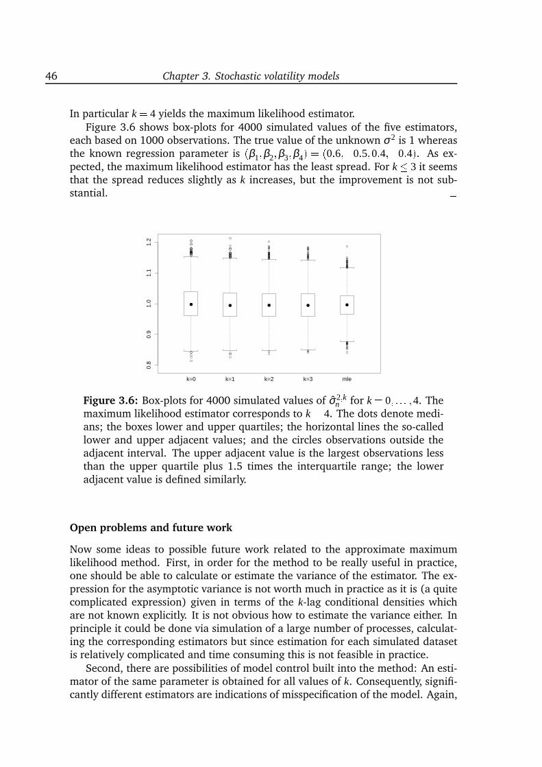
46 Chapter 3. Stochastic volatility models
In particular k = 4 yields the maximum likelihood estimator.Figure 3.6 shows box-plots for 4000 simulated values of the five estimators,
each based on 1000 observations. The true value of the unknown σ2 is 1 whereasthe known regression parameter is (β1;β2;β3;β4) = (0:6;0:5;0:4;0:4). As ex-pected, the maximum likelihood estimator has the least spread. For k 3 it seemsthat the spread reduces slightly as k increases, but the improvement is not sub-stantial.
0.8
0.9
1.0
1.1
1.2
k=0 k=1 k=2 k=3 mle
Figure 3.6: Box-plots for 4000 simulated values of σ2;kn for k = 0; : : : ;4. The
maximum likelihood estimator corresponds to k = 4. The dots denote medi-ans; the boxes lower and upper quartiles; the horizontal lines the so-calledlower and upper adjacent values; and the circles observations outside theadjacent interval. The upper adjacent value is the largest observations lessthan the upper quartile plus 1.5 times the interquartile range; the loweradjacent value is defined similarly.
Open problems and future work
Now some ideas to possible future work related to the approximate maximumlikelihood method. First, in order for the method to be really useful in practice,one should be able to calculate or estimate the variance of the estimator. The ex-pression for the asymptotic variance is not worth much in practice as it is (a quitecomplicated expression) given in terms of the k-lag conditional densities whichare not known explicitly. It is not obvious how to estimate the variance either. Inprinciple it could be done via simulation of a large number of processes, calculat-ing the corresponding estimators but since estimation for each simulated datasetis relatively complicated and time consuming this is not feasible in practice.
Second, there are possibilities of model control built into the method: An esti-mator of the same parameter is obtained for all values of k. Consequently, signifi-cantly different estimators are indications of misspecification of the model. Again,
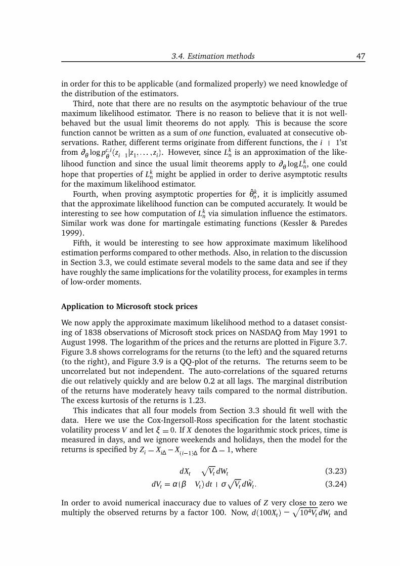
3.4. Estimation methods 47
in order for this to be applicable (and formalized properly) we need knowledge ofthe distribution of the estimators.
Third, note that there are no results on the asymptotic behaviour of the truemaximum likelihood estimator. There is no reason to believe that it is not well-behaved but the usual limit theorems do not apply. This is because the scorefunction cannot be written as a sum of one function, evaluated at consecutive ob-servations. Rather, different terms originate from different functions, the i + 1’stfrom ∂θ logpc;i
θ (zi+1jz1; : : : ;zi). However, since Lkn is an approximation of the like-
lihood function and since the usual limit theorems apply to ∂θ logLkn, one could
hope that properties of Lkn might be applied in order to derive asymptotic results
for the maximum likelihood estimator.Fourth, when proving asymptotic properties for θ k
n , it is implicitly assumedthat the approximate likelihood function can be computed accurately. It would beinteresting to see how computation of Lk
n via simulation influence the estimators.Similar work was done for martingale estimating functions (Kessler & Paredes1999).
Fifth, it would be interesting to see how approximate maximum likelihoodestimation performs compared to other methods. Also, in relation to the discussionin Section 3.3, we could estimate several models to the same data and see if theyhave roughly the same implications for the volatility process, for examples in termsof low-order moments.
Application to Microsoft stock prices
We now apply the approximate maximum likelihood method to a dataset consist-ing of 1838 observations of Microsoft stock prices on NASDAQ from May 1991 toAugust 1998. The logarithm of the prices and the returns are plotted in Figure 3.7.Figure 3.8 shows correlograms for the returns (to the left) and the squared returns(to the right), and Figure 3.9 is a QQ-plot of the returns. The returns seem to beuncorrelated but not independent. The auto-correlations of the squared returnsdie out relatively quickly and are below 0.2 at all lags. The marginal distributionof the returns have moderately heavy tails compared to the normal distribution.The excess kurtosis of the returns is 1.23.
This indicates that all four models from Section 3.3 should fit well with thedata. Here we use the Cox-Ingersoll-Ross specification for the latent stochasticvolatility process V and let ξ 0. If X denotes the logarithmic stock prices, time ismeasured in days, and we ignore weekends and holidays, then the model for thereturns is specified by Zi = Xi∆X(i1)∆ for ∆ = 1, where
dXt =pVt dWt (3.23)
dVt = α(β Vt)dt +σp
Vt dWt : (3.24)
In order to avoid numerical inaccuracy due to values of Z very close to zero wemultiply the observed returns by a factor 100. Now, d(100Xt) =p104Vt dWt and
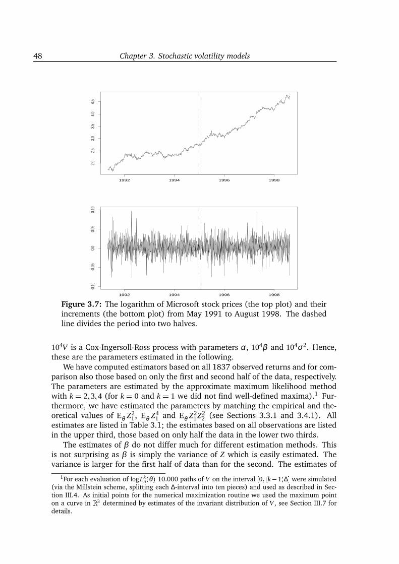
48 Chapter 3. Stochastic volatility models
1992 1994 1996 1998
2.02.5
3.03.5
4.04.5
1992 1994 1996 1998
-0.10
-0.05
0.00.0
50.1
0
Figure 3.7: The logarithm of Microsoft stock prices (the top plot) and theirincrements (the bottom plot) from May 1991 to August 1998. The dashedline divides the period into two halves.
104V is a Cox-Ingersoll-Ross process with parameters α, 104β and 104σ2. Hence,these are the parameters estimated in the following.
We have computed estimators based on all 1837 observed returns and for com-parison also those based on only the first and second half of the data, respectively.The parameters are estimated by the approximate maximum likelihood methodwith k = 2;3;4 (for k = 0 and k = 1 we did not find well-defined maxima).1 Fur-thermore, we have estimated the parameters by matching the empirical and the-oretical values of Eθ Z2
1, Eθ Z41 and Eθ Z2
1Z22 (see Sections 3.3.1 and 3.4.1). All
estimates are listed in Table 3.1; the estimates based on all observations are listedin the upper third, those based on only half the data in the lower two thirds.
The estimates of β do not differ much for different estimation methods. Thisis not surprising as β is simply the variance of Z which is easily estimated. Thevariance is larger for the first half of data than for the second. The estimates of
1For each evaluation of logLkn(θ ) 10.000 paths of V on the interval [0;(k+1)∆ were simulated
(via the Millstein scheme, splitting each ∆-interval into ten pieces) and used as described in Sec-tion III.4. As initial points for the numerical maximization routine we used the maximum pointon a curve in R3 determined by estimates of the invariant distribution of V , see Section III.7 fordetails.
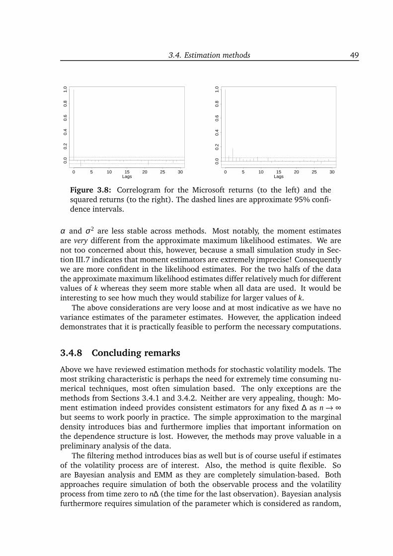
3.4. Estimation methods 49
Lags0 5 10 15 20 25 30
0.0
0.2
0.4
0.6
0.8
1.0
Lags0 5 10 15 20 25 30
0.0
0.2
0.4
0.6
0.8
1.0
Figure 3.8: Correlogram for the Microsoft returns (to the left) and thesquared returns (to the right). The dashed lines are approximate 95% confi-dence intervals.
α and σ2 are less stable across methods. Most notably, the moment estimatesare very different from the approximate maximum likelihood estimates. We arenot too concerned about this, however, because a small simulation study in Sec-tion III.7 indicates that moment estimators are extremely imprecise! Consequentlywe are more confident in the likelihood estimates. For the two halfs of the datathe approximate maximum likelihood estimates differ relatively much for differentvalues of k whereas they seem more stable when all data are used. It would beinteresting to see how much they would stabilize for larger values of k.
The above considerations are very loose and at most indicative as we have novariance estimates of the parameter estimates. However, the application indeeddemonstrates that it is practically feasible to perform the necessary computations.
3.4.8 Concluding remarks
Above we have reviewed estimation methods for stochastic volatility models. Themost striking characteristic is perhaps the need for extremely time consuming nu-merical techniques, most often simulation based. The only exceptions are themethods from Sections 3.4.1 and 3.4.2. Neither are very appealing, though: Mo-ment estimation indeed provides consistent estimators for any fixed ∆ as n ! ∞but seems to work poorly in practice. The simple approximation to the marginaldensity introduces bias and furthermore implies that important information onthe dependence structure is lost. However, the methods may prove valuable in apreliminary analysis of the data.
The filtering method introduces bias as well but is of course useful if estimatesof the volatility process are of interest. Also, the method is quite flexible. Soare Bayesian analysis and EMM as they are completely simulation-based. Bothapproaches require simulation of both the observable process and the volatilityprocess from time zero to n∆ (the time for the last observation). Bayesian analysisfurthermore requires simulation of the parameter which is considered as random,
50 Chapter 3. Stochastic volatility models
Quantiles of Standard Normal
-2 0 2
-0.1
0-0
.05
0.0
0.05
0.10
Figure 3.9: QQ-plot for the Microsoft returns with the quantiles of the nor-mal distribution on the x-axis and quantiles of the returns on the y-axis.
and simulation is performed conditional on the observations. In both cases thesimulations correct for bias but the estimators are bound to depend on the priordistribution of θ (in the Bayesian analysis) or the auxiliary model (in EMM) whichare both selected quite arbitrarily.
Prediction-based estimating functions and the approximate maximum likeli-hood method provide consistent estimators as well. It is often natural to usepredictions based on k lags of the data for some k. In that sense prediction-based estimation is in line with the approximate maximum likelihood method.For fixed k, the functional generating the prediction-based estimating function ischosen slightly arbitrarily (as low order polynomials, say). As opposed to this, theapproximate maximum likelihood method suggests always to use the score cor-responding to the k-lag conditional density. This makes the method invariant todata transformations but, admittedly, it need not provide efficient estimators. Thek’th approximation to the likelihood is computed by simulation, but only of thevolatility process and only at the interval from zero to (k+1)∆. Hence, the com-putational effort needed is presumably considerably smaller than for the Bayesianand auxiliary-based approaches.
3.5 Related models
So far we have been concerned with continuous-time models driven by Brownianmotions. We now discuss related models. First we discuss continuous-time modelsdriven by general Lévy processes, next models defined in discrete time.
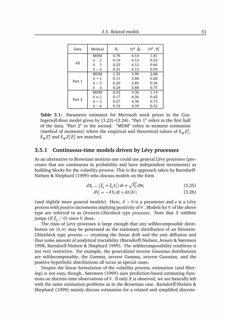
3.5. Related models 51
Data Method αn 104 βn 104 σ2n
MOM 0.76 4.14 1.81
Allk = 2 0.19 4.13 0.53k = 3 0.23 4.12 0.66k = 4 0.21 4.13 0.59MOM 1.35 3.90 2.88
Part 1k = 2 0.11 3.88 0.28k = 3 0.20 3.89 0.58k = 4 0.24 3.88 0.75MOM 0.42 4.36 1.14
Part 2k = 2 0.17 4.36 0.42k = 3 0.27 4.36 0.73k = 4 0.19 4.39 0.52
Table 3.1: Parameter estimates for Microsoft stock prices in the Cox-Ingersoll-Ross model given by (3.23)–(3.24). “Part 1” refers to the first halfof the data, “Part 2” to the second. “MOM” refers to moment estimation(method of moments) where the empirical and theoretical values of Eθ Z2
1,Eθ Z4
1 and Eθ Z21Z2
2 are matched.
3.5.1 Continuous-time models driven by Lévy processes
As an alternative to Brownian motions one could use general Lévy processes (pro-cesses that are continuous in probability and have independent increments) asbuilding blocks for the volatility process. This is the approach taken by Barndorff-Nielsen & Shephard (1999) who discuss models on the form
dXt = ξ1+ξ2Vt
dt +pVt dWt (3.25)
dVt =λVt dt +dz(λ t) (3.26)
(and slightly more general models). Here, λ > 0 is a parameter and z is a Lévyprocess with positive increments implying positivity of V . Models for V of the abovetype are referred to as Ornstein-Uhlenbeck type processes. Note that X exhibitsjumps (if ξ2 6= 0) since V does.
The class of Levy processes is large enough that any selfdecomposable distri-bution on (0;∞) may be generated as the stationary distribution of an Ornstein-Uhlenbeck type process — retaining the linear drift and the unit diffusion andthus some amount of analytical tractability (Barndorff-Nielsen, Jensen & Sørensen1998, Barndorff-Nielsen & Shephard 1999). The selfdecomposability condition isnot very restrictive. For example, the generalized inverse Gaussian distributionsare selfdecomposable; the Gamma, inverse Gamma, inverse Gaussian, and thepositive hyperbolic distributions all occur as special cases.
Despite the linear formulation of the volatility process, estimation (and filter-ing) is not easy, though. Sørensen (1999) uses prediction-based estimating func-tions on discrete-time observations of V . If only X is observed, we are basically leftwith the same estimation problems as in the Brownian case. Barndorff-Nielsen &Shephard (1999) mainly discuss estimation for a related and simplified discrete-
52 Chapter 3. Stochastic volatility models
time model and focus on two filtering approaches and on Bayesian analysis. Thetwo filtering methods carry over to a simplified version of the above continuous-time model (with ξ1 = ξ2 = 0). The possibility of parameter estimation via spectralanalysis is also mentioned.
3.5.2 Related discrete-time models
So far we have been concerned with models that are defined in continuous timebut observed at discrete time-points only. Another possibility is of course to di-rectly define models in discrete time. Such models are often easier to interpret asthey usually specify movements from observation to observation in a relatively di-rect way. On the other hand, continuous-time modeling has advantages: First, thetheory of derivative pricing, for example, most often relies on stochastic calculus.Second, it is easier to handle irregularly sampled data as a continuous-time modelimplicitly defines transitions over time intervals of any length, whereas in discretetime one would have to specify separate (though coherent) models for differenttime intervals.
Apart from being important models in their own right the discrete-time ver-sions may serve as approximations to the continuous-time models (for example, ifestimation is performed by indirect inference or EMM). Or the other way around:the continuous-time versions may be interpreted as limits of discrete-time modelsas the time interval between observations gets smaller (Nelson 1990).
Essentially, discrete-time models of changing variance are given by an equationfor the observations
Yi = µi +σiεi; i = 1; : : : ;n;together with models for the mean µi and variance σi. We let µi 0 as we shallmainly be interested in the variance structure. The innovations (εi)i are assumedto be white noise (e.g. Gaussian) with unit variance. The models can roughlybe divided into two groups: ARCH type models and stochastic volatility mod-els. We refer to survey papers for a thorough treatment of similarities and differ-ences between the two discrete-time type models (Shephard 1996) and betweenthe continuous-time and discrete-time versions of the stochastic volatility models(Ghysels et al. 1996).
ARCH type models
In ARCH type models (εi)i is the only source of noise and σi is assumed to bea (non-random) function of lagged values of Y and σ2. Consequently, the condi-tional distribution of Yi given the past is directly specified and it is straightforward,at least in principle, to do maximum likelihood estimation. Note that although theARCH type models are driven by one source of noise only, their continuous-timelimits (defined in a certain sense, see Nelson (1990)) can be stochastic volatil-ity models of the type from this chapter. For example, the GARCH(1,1) modelconverges to the inverse Gamma model from Section 3.3.1.
3.5. Related models 53
There is a vast literature on ARCH type models, their applications and relatedstatistical issues, and it is beyond the scope of this thesis to go into this. See Bera& Higgins (1993), for example, for a survey of the ARCH literature.
Stochastic volatility models
In the stochastic volatility set-up (σi)i is assumed to evolve independently from— or at least not to be perfectly correlated with — (εi)i. For simplicity we shallconsider a particular model that by far is the most popular model in the literature:assume that σ2
i = exp(Hi) where (Hi)i is an auto-regressive process of order one,
Yi = εi exp(Hi=2)Hi = γ0+ γ1Hi1+ηi;
where the sequences (εi)i and (ηi)i are Gaussian white noise with variances 1 andσ2
η respectively, independent of each other. This model is the natural discrete-timecounterpart of the geometric Ornstein-Uhlenbeck model from Section 3.3.2.
We are interested in estimation of θ = (γ0;γ1;σ2η) from observations (y1; : : : ;yn)
of (Y1; : : : ;Yn). The methods from Section 3.4 are all applicable (when suitablymodified) — and most of them have actually been applied. Not surprisingly mo-ment estimation (generalized method of moments and simulated versions likeEMM) has been popular: Andersen & Sørensen (1996), among many others, ap-ply GMM, and Gallant, Hsieh & Tauchen (1997) apply EMM to the above model.Markov Chain Monte Carlo methods for stochastic volatilities were developed andapplied by Jacquier, Polson & Rossi (1994) and later refined by Kim, Shephard& Chib (1998). The so-called quasi maximum likelihood estimator (Harvey, Ruiz& Shephard 1994) relies on the Kalman filter which is applied to the linear statespace model for logY 2
i : logY 2i = Hi + logε2
i . This yields consistent (but inefficient)parameter estimates although logε2
i is not Gaussian. The above list of applicationsis only a small selection; we refer to the survey papers by Shephard (1996) andGhysels et al. (1996) for many more references.
Maximum likelihood estimation is not possible — for the exact same reasonsas in continuous time: the likelihood is given only in integral form
Ln(θ) = ZRnf (yjh) fθ (h)dh = Eθ f (yjH)
where we have written y for the vector (y1; : : : ;yn) and similarly for h and H andused f generically for densities. Note that the density fθ (h) is actually explicitlyknown. As in continuous time the likelihood could in principle be computed as theaverage of simulated values of f (yjH) where H are simulated from fθ (h). Again,this is not feasible in practice as a huge number of simulations would be necessary.
The new approximate maximum likelihood method from Section 3.4.7 andPaper III is one way to circumvent the problem. The methodology immediatelycarries over to the discrete-time set-up, and simulation of the k-lag conditionaldensities is much easier than in the continuous-time case because the distribution
54 Chapter 3. Stochastic volatility models
of the conditional variances is known explicitly. Note that the method for k = 0(pretending independence) only provides estimates of the parameters γ0=(1 γ1)and σ2
η=(1 γ21) determining the invariant distribution of H.
Another answer is importance sampling. Basically, the idea is to choose a func-tion gy;θ that satisfies
Rgy;θ (h)dh = 1 for all θ and rewrite the likelihood to
Ln(θ) = ZRn
f (yjh) fθ (h)gy;θ (h) gy;θ (h)dh = Ey;θ f (yjh) fθ (h)
gy;θ (h) (3.27)
where Ey;θ is the expectation corresponding to the density gy;θ . Then the likeli-
hood may be calculated as the average of simulated values of f (yjH) fθ (H)=gy;θ (H)where H is drawn from gy;θ .
The question is of course how to choose the density gy;θ cleverly, i.e. such
that relatively few simulations are necessary. Danielsson & Richard (1993) andDanielsson (1994) suggest a product of univariate Gaussian densities. In eachterm the Gaussian mean and variance depend on some auxiliary parameters whichare estimated beforehand in order to obtain the largest possible variance reduc-tion. The technique reduces the number of required simulations of H impressively.Danielsson (1994) applies the technique to a dataset of roughly 2000 observations(and a somewhat more complicated model than the above) and obtains conver-gence using only 5000 simulations. However, the method requires heavy com-putations for estimation of the auxiliary parameters and is still very computerintensive.
Finally, note that it is absolutely crucial that the density of H is known explicitly.Otherwise, the integrand in (3.27) is not known. Hence, the importance samplingapproach cannot immediately be modified to cover the continuous-time modelswhere the distribution of the conditional variances (S1; : : : ;Sn) is not known.
3.6 Conclusion
In this chapter (and in Paper III) we have studied a class of continuous-timestochastic volatility models, mainly from a statistical point of view. The mainconclusion are the following (see Section 3.3.3 and Section 3.4.8 for more de-tailed conclusions). An investigation of four particular models showed differencesin their ability to generate data with highly leptokurtic distributions. In other re-spects the models were hard to distinguish. A new estimation method based onsimulated approximations to the likelihood function was derived. The methodprovides consistent and asymptotically normal estimators for any time distancebetween observations. There are other methods with the same properties, someof which are more widely applicable. However, for the models from this chapterthe new technique provides very natural approximations to the likelihood and isthus quite appealing.
IDiscretely Observed Diffusions:
Approximation of the
Continuous-time Score Function
Abstract
We discuss parameter estimation for discretely observed, ergodic diffusion pro-cesses where the diffusion coefficient does not depend on the parameter. We pro-pose using an approximation of the continuous-time score function as an estimat-ing function. The estimating function can be expressed in simple terms throughthe drift and the diffusion coefficient and is thus easy to calculate. Simulationstudies show that the method performs well.
Key words
Continuous-time score function; diffusion process; discrete observations; estimat-ing function.
Publication details
This paper has been accepted for publication in Scandinavian Journal of Statistics.An earlier version was printed as Preprint no. 8, 1998 at Department of Theoret-ical Statistics, University of Copenhagen (Sørensen 1998a). In this version a fewnotational changes have been made.
56 Paper I. Approximation of the Score Function
I.1 Introduction
This paper is about parameter estimation for discretely observed diffusion mod-els with known diffusion function. The idea is to use an approximation of thecontinuous-time score function as estimating function.
This idea is very much in the spirit of the early work by Le Breton (1976) andFlorens-Zmirou (1989). They both studied the usual Riemann-Itô discretization ofthe continuous-time log-likelihood function, and Florens-Zmirou (1989) showedthat the corresponding estimator is inconsistent when the length of the time inter-val between observations is constant.
More recently, various methods providing consistent estimators have been de-veloped, e.g. methods based on approximations of the true, discrete-time likeli-hood function (Pedersen 1995b, Aït-Sahalia 1998); methods based on auxiliarymodels (Gallant & Tauchen 1996, Gourieroux et al. 1993); and methods basedon estimating functions (Bibby & Sørensen 1995, Hansen & Scheinkman 1995,Kessler 2000, Jacobsen 1998).
The estimating function discussed in this paper is of the simple, explicit typediscussed by Hansen & Scheinkman (1995) and Kessler (2000), that is, on theform ∑n
i=1Aθ h(Xti1;θ) whereAθ is the diffusion generator. Hansen & Scheinkman
(1995) focus on identifiability and asymptotic behaviour of the estimating func-tion whereas Kessler (2000) focuses on asymptotic behaviour and efficiency of theestimator.
The main contribution of this paper is to recognize that, with a special choice ofh, the corresponding estimating function can be interpreted as an approximationto the continuous-time score function. The approximating estimating function isunbiased, it is invariant to data transformations, it provides consistent and asymp-totically normal estimators, and it can be explicitly expressed in terms of the driftand diffusion coefficient. The estimating function is also — at least in some cases— available for multi-dimensional processes.
The main objection against the method is the need for a completely known dif-fusion function. In case of a parameter dependent diffusion function the suggestedestimating function is still unbiased and can thus in principle be used, but thereis no longer justification for using it since the continuous-time likelihood functiondoes not exist.
We present the model and the basic assumptions in Section I.2, and the estimat-ing function is derived in Section I.3. We give the asymptotic results in Section I.4,and examples and simulation studies in Section I.5. Sections I.2–I.5 discuss one-dimensional diffusion processes exclusively; we study the multi-dimensional casein Section I.6.
I.2 Model and notation
In this section we present the diffusion model, state the assumptions and introducesome notation.
(I.2)
I.3. The estimating function 57
We consider the one-dimensional, time-homogeneous stochastic differentialequation
dXt = b(Xt;θ)dt +σ(Xt)dWt ; X0 = x0 (I.1)
where θ is an unknown p-dimensional parameter from the parameter space Θ Rp and W is a one-dimensional Brownian motion. The functions b : RΘ ! R andσ : R ! (0;∞) are known, and the derivatives ∂σ=∂x and ∂ 2b=∂θ j∂x are assumedto exist for all j = 1; : : : ; p. Note that σ does not depend on θ .
We assume that for any θ , (I.1) has a unique, strong solution X and that therange of X does not depend on θ . Assume furthermore that there exists a uniqueinvariant distribution µθ = µ(x;θ)dx such that a solution to (I.1) with X0 µθ (in-stead of X0 = x0) is strictly stationary. Sufficient conditions for these assumptionsto hold can be found in Karatzas & Shreve (1991).
The invariant density is given by
µ(x;θ) = C(θ)s(x;θ)σ2(x)1(I.2)
where C(θ) is a normalizing constant and s(;θ) is the density of the scale measure,i.e. logs(x;θ) =2
R x b(y;θ)=σ2(y)dy:For all θ 2 Θ, the distribution of X is denoted Pθ if X0 = x0 (as in (I.1)) and Pµ
θif X0 µθ .1 Under Pµ
θ all Xt µθ . Eµθ is the expectation wrt. Pµ
θ .
The objective is to estimate θ from observations of X at discrete time-pointst1 < < tn. Define t0 = 0 and ∆i = ti ti1 and let θ0 be the true parameter.
Finally, we need some matrix notation: Vectors in Rp are considered as p1matrices, and AT is the transpose of A. For a function f = ( f1; : : : ; fq)T : RΘ !Rq we let f 0(x;θ) be the q1 matrix of partial derivatives with respect to x andf (x;θ) = Dθ f (x;θ) be the q p matrix of partial derivatives with respect to θ , i.e.
f jk = ∂ f j=∂θk.
I.3 The estimating function
In this section we derive a simple, unbiased estimating function as an approxima-tion of the continuous-time score function.
First a comment on the model: It is important that σ does not depend on θ .Otherwise the distributions of (Xs)0st corresponding to two different parametervalues are typically singular for all t 0. If Y is the solution to dYt = b(Yt ;θ)dt +σ(Yt ;θ)dWt , then the process (R Yt 1=σ(y;θ)dy)t0 is the solution to (I.1) with σ 1,but this is of no help for estimation purposes since the transformation depends onthe (unknown) parameter.
1Note the difference in notation from Chapter 2 and Paper II where Pθ is the distribution of Xwhen X0 is started according to the stationary distribution (and where we have no notation for thedistribution of X given a particular value of X0).
(I.3)
58 Paper I. Approximation of the Score Function
When σ is completely known as we have assumed, it follows from Lipster& Shiryayev (1977) that the likelihood function for a continuous observation(Xs)0st exists and that the corresponding score process Sc is given by
Sct (θ) = Z t
0
b(Xs;θ)σ2(Xs) dXsZ t
0
b(Xs;θ)b(Xs;θ)σ2(Xs) ds:
Using (I.1) we find that
dSct (θ) = b(Xt;θ)
σ(Xt) dWt : (I.3)
This shows that Sc(θ) is a local martingale and that it is a genuine martingale ifEµ
θR t
0(b j(Xs;θ)=σ(Xs))2ds < ∞ for all t 0 and all j = 1; : : : ; p, i.e. if
Eµθ
b j(X0;θ)
σ(X0) 2 = Z b j(x;θ)σ(x) 2
µ(x;θ)dx < ∞ (I.4)
for all j = 1; : : : ; p. In particular, Eµθ Sc
t = 0 for all t 0 if (I.4) holds.
If X was observed continuously on the interval [0; tn we would estimate θ bysolving the equation Sc
tn(θ) = 0. For discrete observations at time-points t1; : : : ; tn,the idea is to use an approximation of Sc
tn as estimating function.The most obvious approximation is obtained by simply replacing the integrals
in (I.3) with the corresponding Riemann and Itô sums,
Rn(θ) = n
∑i=1
b(Xti1;θ)
σ2(Xti1) Xti
Xti1
n
∑i=1
∆i
b(Xti1;θ)b(Xti1
;θ)σ2(Xti1
) : (I.5)
Note that this would be the score function if the conditional distributions of theincrements Xti
Xti1, given the past, were Gaussian with expectation ∆ib(Xti1
;θ)and variance ∆iσ
2(Xti1). However, usually Eµ
θ Rn(θ) 6= 0, and Rn provides inconsis-
tent estimators unless supi=1;::: ;n ∆i ! 0 (Florens-Zmirou 1989).We now propose an unbiased approximation of Sc
tn. Let Aθ denote the differ-ential operator associated with the infinitesimal generator for X , that is,Aθ f (x;θ) = b(x;θ) f 0(x;θ)+ 1
2σ2(x) f 00(x;θ)
for functions f : RΘ ! Rp that are twice continuously differentiable wrt. x.Recall that µ is the invariant density and assume that the derivatives
h? = Dθ logµ : RΘ ! Rp
wrt. the coordinates of θ exist and are twice continuously differentiable wrt. x,such that Aθ h? is well-defined. The connection between h? and Sc is given in thefollowing proposition:
(I.4)
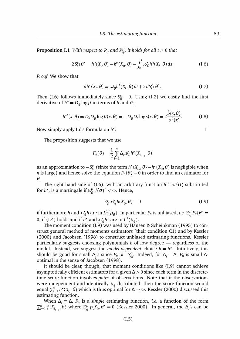
I.3. The estimating function 59
Proposition I.1 With respect to Pθ and Pµθ , it holds for all t 0 that
2Sct (θ) = h?(Xt;θ)h?(X0;θ)Z t
0Aθ h?(Xs;θ)ds: (I.6)
Proof We show that
dh?(Xt;θ) =Aθ h?(Xt ;θ)dt +2dSct (θ): (I.7)
Then (I.6) follows immediately since Sc0 = 0. Using (I.2) we easily find the first
derivative of h? = Dθ logµ in terms of b and σ ;
h?0(x;θ) = DxDθ logµ(x;θ) =Dθ Dx logs(x;θ) = 2b(x;θ)σ2(x) : (I.8)
Now simply apply Itô’s formula on h?. The proposition suggests that we use
Fn(θ) = 12
n
∑i=1
∆iAθ h?(Xti1;θ)
as an approximation to Sctn (since the term h?(Xtn;θ)h?(X0;θ) is negligible when
n is large) and hence solve the equation Fn(θ) = 0 in order to find an estimator forθ .
The right hand side of (I.6), with an arbitrary function h 2 C 2(I) substitutedfor h?, is a martingale if Eµ
θ (h0σ)2 < ∞. Hence,
Eµθ Aθ h(X0;θ) = 0 (I.9)
if furthermore h andAθ h are in L1(µθ ). In particular Fn is unbiased, i.e. Eµθ Fn(θ) =
0, if (I.4) holds and if h? and Aθ h? are in L1(µθ ).The moment condition (I.9) was used by Hansen & Scheinkman (1995) to con-
struct general method of moments estimators (their condition C1) and by Kessler(2000) and Jacobsen (1998) to construct unbiased estimating functions. Kesslerparticularly suggests choosing polynomials h of low degree — regardless of themodel. Instead, we suggest the model-dependent choice h = h?. Intuitively, thisshould be good for small ∆i’s since Fn Sc
tn. Indeed, for ∆i ∆, Fn is small ∆-optimal in the sense of Jacobsen (1998).
It should be clear, though, that moment conditions like (I.9) cannot achieveasymptotically efficient estimators for a given ∆> 0 since each term in the discrete-time score function involves pairs of observations. Note that if the observationswere independent and identically µθ -distributed, then the score function wouldequal ∑n
i=1 h?(Xti;θ) which is thus optimal for ∆!∞. Kessler (2000) discussed this
estimating function.When ∆i ∆, Fn is a simple estimating function, i.e. a function of the form
∑ni=1 f (Xti1
;θ) where Eµθ f (X0;θ) = 0 (Kessler 2000). In general, the ∆i’s can be
(I.5)
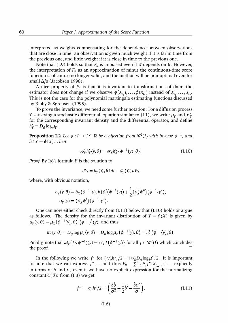
60 Paper I. Approximation of the Score Function
interpreted as weights compensating for the dependence between observationsthat are close in time: an observation is given much weight if it is far in time fromthe previous one, and little weight if it is close in time to the previous one.
Note that (I.9) holds so that Fn is unbiased even if σ depends on θ . However,the interpretation of Fn as an approximation of minus the continuous-time scorefunction is of course no longer valid, and the method will be non-optimal even forsmall ∆i’s (Jacobsen 1998).
A nice property of Fn is that it is invariant to transformations of data; theestimator does not change if we observe ϕ(Xt1
); : : : ;ϕ(Xtn) instead of Xt1; : : : ;Xtn.
This is not the case for the polynomial martingale estimating functions discussedby Bibby & Sørensen (1995).
To prove the invariance, we need some further notation: For a diffusion processY satisfying a stochastic differential equation similar to (I.1), we write µY and AYfor the corresponding invariant density and the differential operator, and defineh?
Y = Dθ logµY .
Proposition I.2 Let ϕ : I ! J R be a bijection from C 2(I) with inverse ϕ1, and
let Y = ϕ(X). Then AY h?Y (y;θ) =AX h?
X
ϕ1(y);θ: (I.10)
Proof By Itô’s formula Y is the solution to
dYt = bY (Yt ;θ)dt +σY (Yt)dWt
where, with obvious notation,
bY (y;θ) = bX
ϕ1(y);θϕ 0ϕ1(y)+ 1
2
σ2
X ϕ 00ϕ1(y);σY (y) = σX ϕ 0ϕ1(y):
One can now either check directly from (I.11) below that (I.10) holds or argueas follows. The density for the invariant distribution of Y = ϕ(X) is given by
µY (y;θ) = µX
ϕ1(y);θϕ1
0 (y) and thus
h?Y (y;θ) = Dθ logµY (y;θ) = Dθ logµX
ϕ1(y);θ= h?
X
ϕ1(y);θ:
Finally, note that AY ( f Æϕ1)(y) =AX fϕ1(y) for all f 2 C 2(I) which concludes
the proof. In the following we write f ? for (Aθ h?)=2 = (Aθ Dθ logµ)=2. It is important
to note that we can express f ? — and thus Fn = ∑ni=1∆i f ?(Xti1
; ) — explicitly
in terms of b and σ , even if we have no explicit expression for the normalizingconstant C(θ): from (I.8) we get
f ? =Aθ h?=2= bbσ2 + 1
2b0 bσ 0
σ
: (I.11)
(I.6)
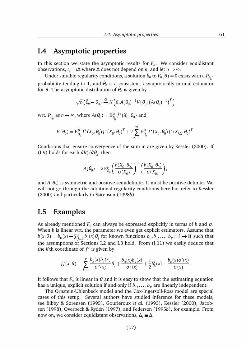
I.4. Asymptotic properties 61
I.4 Asymptotic properties
In this section we state the asymptotic results for Fn. We consider equidistantobservations, ti = i∆ where ∆ does not depend on n, and let n!∞.
Under suitable regularity conditions, a solution θn to Fn(θ)= 0 exists with a Pθ0-
probability tending to 1, and θn is a consistent, asymptotically normal estimatorfor θ . The asymptotic distribution of θn is given byp
nθnθ0
D! N
0;A(θ0)1V (θ0)A(θ0)1T
wrt. Pθ0as n! ∞, where A(θ0) = Eµ
θ0f ?(X0;θ0) and
V (θ0) = Eµθ0
f ?(X0;θ0) f ?(X0;θ0)T +2∞
∑k=1
Eµθ0
f ?(X0;θ0) f ?(Xk∆;θ0)T :Conditions that ensure convergence of the sum in are given by Kessler (2000). If(I.9) holds for each ∂h?
j=∂θk, then
A(θ0) = 2Eµθ0
b(X0;θ0)
σ(X0) T b(X0;θ0)σ(X0) ;
and A(θ0) is symmetric and positive semidefinite. It must be positive definite. Wewill not go through the additional regularity conditions here but refer to Kessler(2000) and particularly to Sørensen (1998b).
I.5 Examples
As already mentioned Fn can always be expressed explicitly in terms of b and σ .When b is linear wrt. the parameter we even get explicit estimators. Assume thatb(x;θ) = b0(x)+∑p
j=1b j(x)θ j for known functions b0;b1; : : : ;bp : R ! R such that
the assumptions of Sections I.2 and I.3 hold. From (I.11) we easily deduce thatthe k’th coordinate of f ? is given by
f ?k (x;θ) = p
∑j=1
bk(x)b j(x)σ2(x) θ j + b0(x)bk(x)
σ2(x) + 12
b0k(x) bk(x)σ 0(x)σ(x) :
It follows that Fn is linear in θ and it is easy to show that the estimating equationhas a unique, explicit solution if and only if b1; : : : ;bp are linearly independent.
The Ornstein-Uhlenbeck model and the Cox-Ingersoll-Ross model are specialcases of this setup. Several authors have studied inference for these models,see Bibby & Sørensen (1995), Gourieroux et al. (1993), Kessler (2000), Jacob-sen (1998), Overbeck & Rydén (1997), and Pedersen (1995b), for example. Fromnow on, we consider equidistant observations, ∆i ∆.
(I.7)
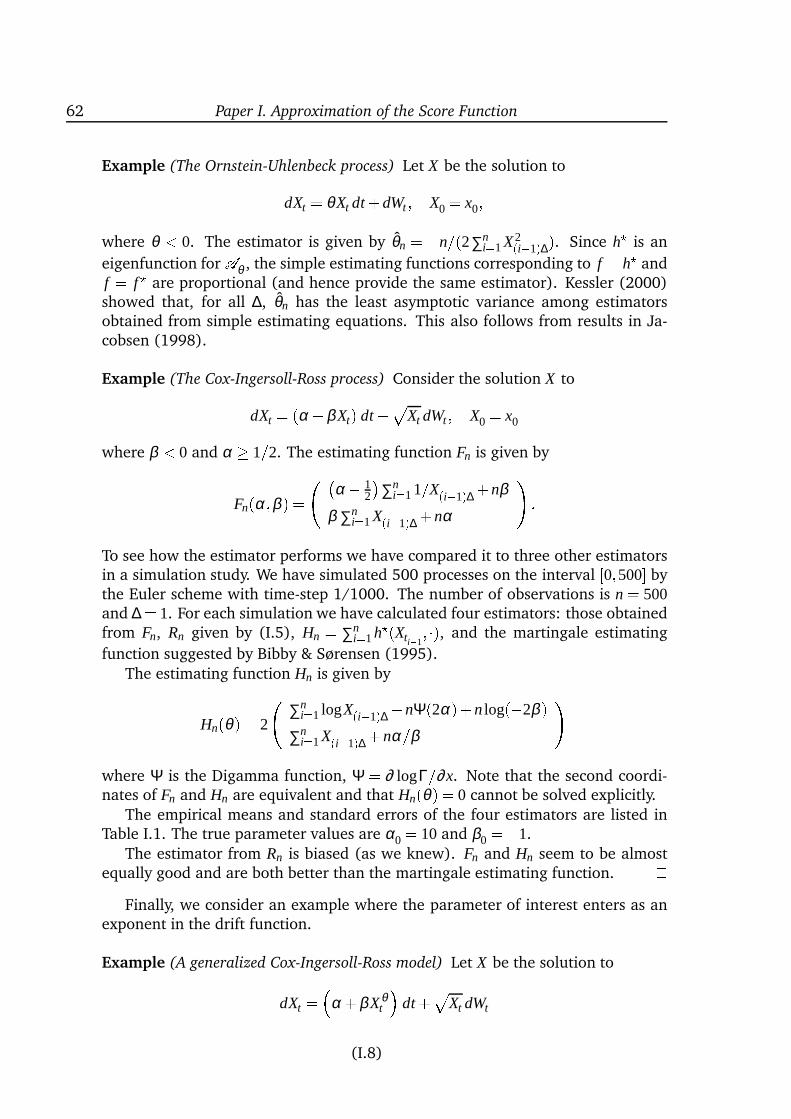
62 Paper I. Approximation of the Score Function
Example (The Ornstein-Uhlenbeck process) Let X be the solution to
dXt = θXt dt +dWt ; X0 = x0;where θ < 0. The estimator is given by θn = n=(2∑n
i=1 X2(i1)∆). Since h? is an
eigenfunction for Aθ , the simple estimating functions corresponding to f = h? andf = f ? are proportional (and hence provide the same estimator). Kessler (2000)showed that, for all ∆, θn has the least asymptotic variance among estimatorsobtained from simple estimating equations. This also follows from results in Ja-cobsen (1998). Example (The Cox-Ingersoll-Ross process) Consider the solution X to
dXt = (α +βXt) dt +pXt dWt ; X0 = x0
where β < 0 and α 1=2. The estimating function Fn is given by
Fn(α;β ) = α 1
2
∑n
i=11=X(i1)∆ +nβ
β ∑ni=1 X(i1)∆ +nα
! :To see how the estimator performs we have compared it to three other estimatorsin a simulation study. We have simulated 500 processes on the interval [0;500 bythe Euler scheme with time-step 1/1000. The number of observations is n = 500and ∆ = 1. For each simulation we have calculated four estimators: those obtainedfrom Fn, Rn given by (I.5), Hn = ∑n
i=1h?(Xti1; ), and the martingale estimating
function suggested by Bibby & Sørensen (1995).The estimating function Hn is given by
Hn(θ) = 2
∑n
i=1 logX(i1)∆nΨ(2α)+n log(2β )∑n
i=1X(i1)∆ +nα=β
!where Ψ is the Digamma function, Ψ = ∂ logΓ=∂x. Note that the second coordi-nates of Fn and Hn are equivalent and that Hn(θ) = 0 cannot be solved explicitly.
The empirical means and standard errors of the four estimators are listed inTable I.1. The true parameter values are α0 = 10 and β0 =1.
The estimator from Rn is biased (as we knew). Fn and Hn seem to be almostequally good and are both better than the martingale estimating function.
Finally, we consider an example where the parameter of interest enters as anexponent in the drift function.
Example (A generalized Cox-Ingersoll-Ross model) Let X be the solution to
dXt = α +βXθt
dt +pXt dWt
(I.8)
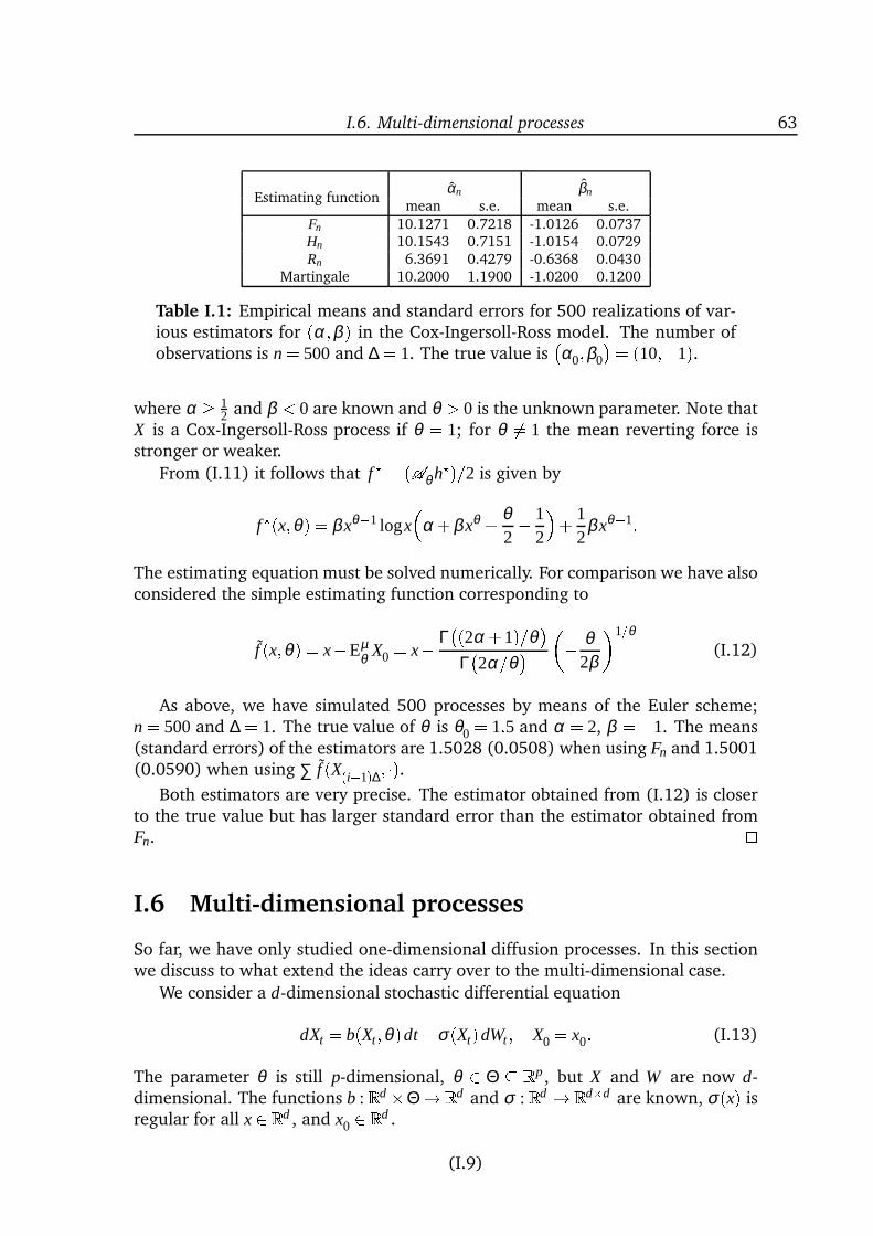
I.6. Multi-dimensional processes 63
Estimating functionαn βn
mean s.e. mean s.e.Fn 10.1271 0.7218 -1.0126 0.0737Hn 10.1543 0.7151 -1.0154 0.0729Rn 6.3691 0.4279 -0.6368 0.0430
Martingale 10.2000 1.1900 -1.0200 0.1200
Table I.1: Empirical means and standard errors for 500 realizations of var-ious estimators for (α;β ) in the Cox-Ingersoll-Ross model. The number ofobservations is n = 500and ∆ = 1. The true value is
α0;β0
= (10;1).where α 1
2 and β < 0 are known and θ > 0 is the unknown parameter. Note thatX is a Cox-Ingersoll-Ross process if θ = 1; for θ 6= 1 the mean reverting force isstronger or weaker.
From (I.11) it follows that f ? = (Aθ h?)=2 is given by
f ?(x;θ) = βxθ1 logx
α +βxθ + θ2 1
2
+ 12
βxθ1:The estimating equation must be solved numerically. For comparison we have alsoconsidered the simple estimating function corresponding to
f (x;θ) = xEµθ X0 = x Γ
(2α +1)=θ
Γ2α=θ
θ2β
1=θ(I.12)
As above, we have simulated 500 processes by means of the Euler scheme;n = 500and ∆ = 1. The true value of θ is θ0 = 1:5 and α = 2, β = 1. The means(standard errors) of the estimators are 1.5028 (0.0508) when using Fn and 1.5001(0.0590) when using ∑ f (X(i1)∆; ).
Both estimators are very precise. The estimator obtained from (I.12) is closerto the true value but has larger standard error than the estimator obtained fromFn. I.6 Multi-dimensional processes
So far, we have only studied one-dimensional diffusion processes. In this sectionwe discuss to what extend the ideas carry over to the multi-dimensional case.
We consider a d-dimensional stochastic differential equation
dXt = b(Xt;θ)dt +σ(Xt)dWt ; X0 = x0: (I.13)
The parameter θ is still p-dimensional, θ 2 Θ Rp , but X and W are now d-dimensional. The functions b : Rd Θ! Rd and σ : Rd ! Rdd are known, σ(x) isregular for all x 2 Rd , and x0 2 Rd .
(I.9)
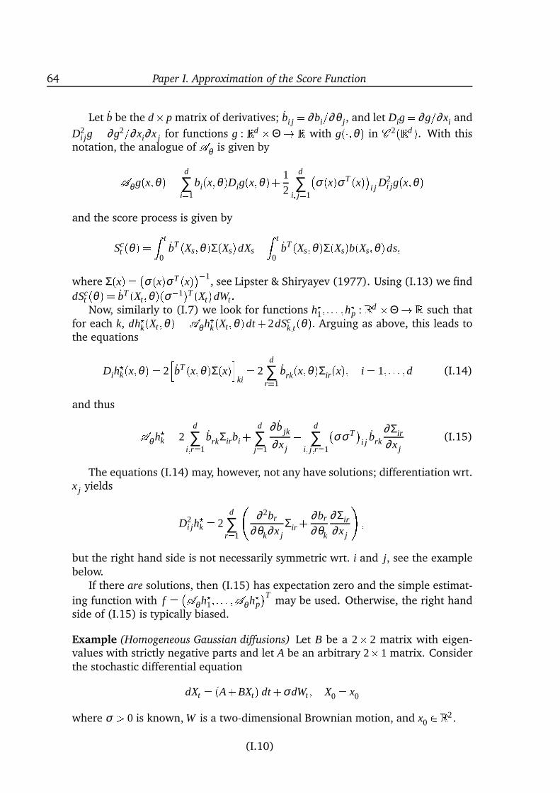
64 Paper I. Approximation of the Score Function
Let b be the d p matrix of derivatives; bi j = ∂bi=∂θ j, and let Dig = ∂g=∂xi and
D2i jg = ∂g2=∂xi∂x j for functions g : Rd Θ ! R with g(;θ) in C 2(Rd ). With this
notation, the analogue of Aθ is given byAθ g(x;θ) = d
∑i=1
bi(x;θ)Dig(x;θ)+ 12
d
∑i; j=1
σ(x)σ T (x)i j D2
i jg(x;θ)and the score process is given by
Sct (θ) = Z t
0bT (Xs;θ)Σ(Xs)dXsZ t
0bT (Xs;θ)Σ(Xs)b(Xs;θ)ds;
where Σ(x) = σ(x)σ T (x)1, see Lipster & Shiryayev (1977). Using (I.13) we find
dSct (θ) = bT (Xt;θ)(σ1)T (Xt)dWt :Now, similarly to (I.7) we look for functions h?
1; : : : ;h?p : Rd Θ ! R such that
for each k, dh?k(Xt ;θ) = Aθ h?
k(Xt;θ)dt +2dSck;t(θ): Arguing as above, this leads to
the equations
Dih?k(x;θ) = 2
hbT (x;θ)Σ(x)i
ki= 2
d
∑r=1
brk(x;θ)Σir(x); i = 1; : : : ;d (I.14)
and thus Aθ h?k = 2
d
∑i;r=1
brkΣirbi + d
∑j=1
∂ b jk
∂x j+ d
∑i; j;r=1
σσ T
i j brk
∂Σir
∂x j(I.15)
The equations (I.14) may, however, not any have solutions; differentiation wrt.x j yields
D2i jh
?k = 2
d
∑r=1
∂ 2br
∂θk∂x jΣir + ∂br
∂θk
∂Σir
∂x j
! ;but the right hand side is not necessarily symmetric wrt. i and j, see the examplebelow.
If there are solutions, then (I.15) has expectation zero and the simple estimat-
ing function with f = Aθ h?1; : : : ;Aθ h?
p
Tmay be used. Otherwise, the right hand
side of (I.15) is typically biased.
Example (Homogeneous Gaussian diffusions) Let B be a 2 2 matrix with eigen-values with strictly negative parts and let A be an arbitrary 21 matrix. Considerthe stochastic differential equation
dXt = (A+BXt) dt +σdWt ; X0 = x0
where σ > 0 is known, W is a two-dimensional Brownian motion, and x0 2 R2.
(I.10)
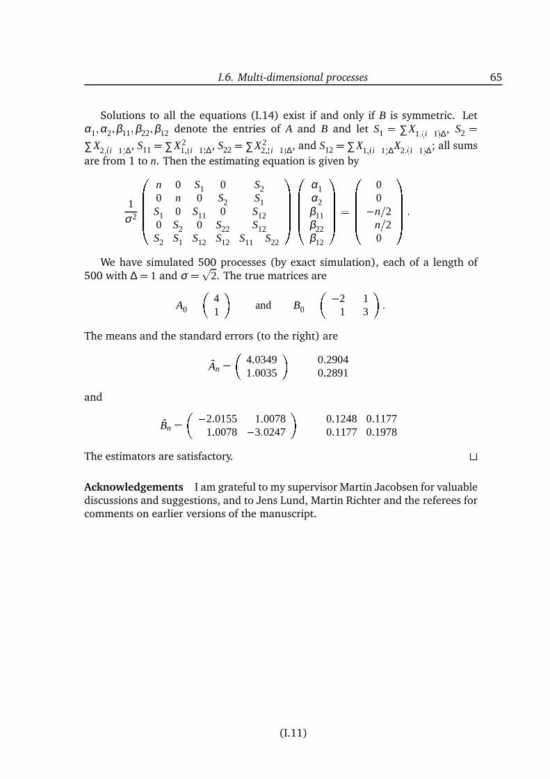
I.6. Multi-dimensional processes 65
Solutions to all the equations (I.14) exist if and only if B is symmetric. Letα1;α2;β11;β22;β12 denote the entries of A and B and let S1 = ∑X1;(i1)∆, S2 =∑X2;(i1)∆, S11 = ∑X2
1;(i1)∆, S22 = ∑X22;(i1)∆, and S12 = ∑X1;(i1)∆X2;(i1)∆; all sums
are from 1 to n. Then the estimating equation is given by
1σ2
0BBBB n 0 S1 0 S20 n 0 S2 S1S1 0 S11 0 S120 S2 0 S22 S12S2 S1 S12 S12 S11+S22
1CCCCA0BBBB α1α2β11β22β12
1CCCCA=0BBBB 00n=2n=20
1CCCCA :We have simulated 500 processes (by exact simulation), each of a length of
500 with ∆ = 1 and σ =p2. The true matrices are
A0 = 41
and B0 = 2 1
1 3
:The means and the standard errors (to the right) are
An = 4:03491:0035
0:29040:2891
and
Bn = 2:0155 1:00781:0078 3:0247
0:1248 0:11770:1177 0:1978
The estimators are satisfactory. Acknowledgements I am grateful to my supervisor Martin Jacobsen for valuablediscussions and suggestions, and to Jens Lund, Martin Richter and the referees forcomments on earlier versions of the manuscript.
(I.11)

IIEstimation of Diffusion Parameters
for Discretely Observed
Diffusion Processes
Abstract
We study estimation of diffusion parameters for one-dimensional, ergodic diffu-sion processes that are discretely observed. We discuss a method based on afunctional relationship between the drift function, the diffusion function and theinvariant density and use empirical process theory to show that the estimator isp
n-consistent and in certain cases weakly convergent. We try out the methodon the so-called CKLS model and compare it with other methods in a simulationstudy.
Key words
CKLS model; diffusion parameters; ergodic diffusion processes; empirical processtheory.
Publication details
A shorter version of this paper has been submitted for publication and was alsoprinted as Preprint no. 1, 2000 at Department of Theoretical Statistics, Univer-sity of Copenhagen (Sørensen 2000). The shorter version does not include Sec-tion II.7.1, the final subsection of Section II.7.2 (Considerations on asymptotics)and the appendices. Furthermore, various parts have been revised slightly in thepresent version.
68 Paper II. Estimation of Diffusion Parameters
II.1 Introduction
This paper is about parametric estimation of the diffusion function for a discretelyobserved diffusion process. The likelihood function is only known analytically invery few cases so it is usually not possible to do maximum likelihood estimation.The method discussed in this paper is inspired by a non-parametric estimationprocedure suggested by Aït-Sahalia (1996) which we shall describe shortly.
Let b be the drift function, σ the diffusion function, and µ the invariant densityfor a one-dimensional diffusion process with state space (l;r). Then, in manycases, there is the connection 2bµ = (σ2µ)0, i.e.
b(x) = 12
σ20(x)+σ2(x)µ 0(x)
µ(x) ; x 2 (l;r) (II.1)
between b, σ and µ, a prime denoting differentiation with respect to the statevariable. This relationship has been used for non-parametric estimation by severalauthors. For σ known Banon (1978) defines an estimator of b(x) for all x in (l;r)(pointwise) by plugging in kernel estimates of µ(x) and µ 0(x). For σ unknown butconstant (so that (σ2)0 = 0) an estimate of σ is plugged in as well. For generalunknown functions σ Jiang & Knight (1997) use local time based estimators of σ2
and (σ2)0, see also Florens-Zmirou (1993).Aït-Sahalia (1996) uses a related but almost opposite estimation strategy in
that he first estimates the drift and next the diffusion function. He assumes thatσ2(x)µ(x)! 0 as x! l and uses the integrated version
σ2(x)µ(x) = 2Z x
lb(u)µ(u)du; x 2 (l;r) (II.2)
of (II.1). He considers linear drift only and uses conditional least squares forestimation of the drift parameters. For each x an estimator of σ2(x) is defined bydividing a kernel estimator of the integral in (II.2) by a kernel estimator of µ(x).
This procedure yields a non-parametric estimator of σ2. The method seems towork well for a large sample size (Aït-Sahalia uses the method on a dataset with5505 observations). For moderate sample sizes, however, the kernel estimatorsand hence the diffusion estimator will be rather variable. Also, if a non-parametricanalysis indicates a certain form of σ2 (e.g. that of a power function), then it isnatural to specify the diffusion parametrically and estimate the parameters. Forparametric specifications it is also possible to verify for which parameter valuesthe relation (II.2) actually holds.
In this paper the relationship (II.2) is utilized for parametric estimation of thediffusion function. The idea is the following. Let f = σ2µ. As we shall see, it iseasy for each x to define a consistent estimator f (x) of f (x;θ). We also have ananalytical expression for f (x;θ), and we estimate θ such that the “true” functionf (;θ) is close to the estimated version f in the sense that the uniform distancesupx2(l;r) f (x;θ) f (x) is minimal. In order for a simple estimator f (x) to exist it
is crucial that f converges to zero at at least one of the endpoints, l and r, of the
(II.2)
II.2. Model and notation 69
state space. We distinguish between three cases: f converges to zero (i) at l only;(ii) at r only; (iii) at both l and r. We use different pointwise consistent estimatorsof f in case (i) and (ii) and a suitable average of the two in case (iii).
The corresponding estimators are consistent under weak regularity conditionsand
pn-consistent under somewhat stronger conditions. In case (iii) the estimator
is weakly convergent. The asymptotic results are proved by means of empiricalprocess theory.
We use the Ornstein-Uhlenbeck process and the so-called CKLS model (Chan,Karolyi, Longstaff & Sanders 1992) for illustration. For the CKLS model givenby dXt = (α + βXt)dt +σX γ
t dWt , we compare the method with other estimationmethods (generalized method of moments, IID estimation, and simple, explicitestimating equations) in a simulation study. The method seems to work well.
The paper is organized as follows. The model and the basic assumptions arepresented in Section II.2. We discuss the estimation approach in Section II.3 andprove asymptotic properties in Sections II.4 and II.5. While in Sections II.3– II.5it is assumed that the drift function is completely known, in Section II.6 we dis-cuss what to do if the drift must be estimated as well. In Section II.7 we studythe Ornstein-Uhlenbeck process and the CKLS model. Conclusions are drawn inSection II.8. In Appendix II.A we give a brief review of the theory of empiricalprocesses which we use to show asymptotic properties for our estimator. Finally,Appendix II.B gives a proof that the Ornstein-Uhlenbeck process is β -mixing at anexponential rate.
II.2 Model and notation
In this section we define the diffusion model and list basic assumptions that ensurenice properties of the model. For details on diffusion processes see Karatzas &Shreve (1991), for example.
We consider the one-dimensional, time-homogeneous stochastic differentialequation
dXt = b(Xt)dt +σ(Xt ;θ)dWt (II.3)
where θ is an unknown p-dimensional parameter from the parameter space Θ Rp , W is a one-dimensional Brownian motion and b : R ! R and σ : RΘ ! R areknown continuous functions.
The objective is estimation of θ from observations X∆; : : : ;Xn∆ at discrete, equi-distant time-points. Let θ0 be the true parameter. Note that the drift function, b,does not depend on the parameter. We will relax this unrealistic condition laterand instead assume that the drift parameters can be estimated without informa-tion on the diffusion parameters, see Section II.6.
We assume that a unique, strong solution to (II.3) exists for all θ 2 Θ and allinitial distributions of X0, that the state space, denoted by I, is the same for allθ 2 Θ and that I is open. Since X is continuous, I is an interval, and we writeI = (l;r) where ∞ l < r +∞.
(II.3)
70 Paper II. Estimation of Diffusion Parameters
We furthermore make assumptions ensuring stationarity of the process: as-sume that σ(x;θ)> 0 for all (x;θ) 2 IΘ and define
s(x;θ) = exp
2Z x
x0
b(y)σ2(y;θ) dy
; (x;θ) 2 IΘ (II.4)
where x0 2 I is arbitrary but fixed. For each θ 2 Θ the function x! R xx0
s(y;θ)dy is
called a scale function.
Assumption II.1 The diffusion function is positive, i.e. σ(x;θ)> 0 for all (x;θ) 2IΘ, and for all θ 2Θ the function s(;θ) satisfies
1.R r
x0s(x;θ)dx = R x0
ls(x;θ)dx =+∞;
2.R r
l
s(x;θ)σ2(x;θ)1
dx < ∞. With these assumptions, X is recurrent (hits any level in I almost surely), does nothit l and r, and has a unique invariant distribution µθ (dx) = µ(x;θ)dx where
µ(x;θ) = K0(θ)s(x;θ)σ2(x)1: (II.5)
The normalizing constant K0(θ) is the inverse of the integral in Assumption II.1.2and depends on the choice of x0.
We let Pθ denote the distribution of X when X0 µθ and Eθ the expecta-tion with respect to Pθ . Under Pθ all Xt µθ and the ergodic theorem holds,
i.e. 1n ∑n
i=1g(Xi∆)! Eθ g(X0) Pθ -almost surely as n ! ∞ for all g 2 L1(µθ ). In thefollowing we shall use the ergodic theorem on the drift function b so we assumethat it is µθ -integrable:
Assumption II.2 The drift function b is in L1(µθ ) for all θ 2 Θ, i.e.R jbjdµθ < ∞
for all θ 2 Θ. The estimation method described in this paper is based on the function f =
σ2µ : IΘ! (0;∞). For θ fixed we will often write fθ for the function f (;θ) : I !R. By (II.5) and (II.4)
fθ (x) = f (x;θ) = K0(θ)s(x;θ) = K0(θ)exp
2Z x
x0
b(u)σ2(u;θ) du
:Differentiation of f with respect to x yields
∂ f∂x
= 2 fb
σ2 = 2σ2µb
σ2 = 2bµ (II.6)
and f (x0;θ) = K0(θ) so f (x;θ) = K0(θ)+2R x
x0b(u)µ(u;θ)du for x 2 I and θ 2 Θ. In
particular, for θ fixed the function fθ is bounded by K0(θ)+2Eθ jb(X0)j; the limits
(II.4)
II.3. Estimation 71
fθ (l) = f (l;θ) = limx&l f (x;θ) and fθ (r) = f (r;θ) = limx%n f (x;θ) are well-defined
and finite; and
f (x;θ) = f (l;θ)+2Z x
lb(u)µ(u;θ)du; x 2 I (II.7)
f (x;θ) = f (r;θ)2Z r
xb(u)µ(u;θ)du; x 2 I: (II.8)
The limits f (l;θ) and f (r;θ) are non-negative for all θ 2Θ. For the estimationmethod below to work at least one of the limits must be zero for all θ 2 Θ. Infor-mally, since f = σ2µ, the assumption is that σ2 does not grow too fast at (at leastone of) the limits. More precisely we must check that
R rx0
b(x)=σ2(x;θ)dx =∞ for
all θ 2Θ and/orR x0
lb(x)=σ2(x;θ)dx =+∞ for all θ 2Θ: In both cases fθ is bounded
by 2Eθ jb(X0)j.Some comments: (i) If l >∞ (r <+∞) then automatically f (l;θ)= 0 ( f (r;θ)=
0) because of Assumption II.1.2. In particular f (l;θ) = 0 for all models with statespace (0;∞). (ii) If I = (∞;∞) and b 0 so X is on natural scale, then fθ isconstant and the above integral assumption is not satisfied. (iii) It follows from(II.7) and (II.8) that f (r;θ) f (l;θ) = 2Eθ b(X0). In particular Eθ b(X0) = 0 if bothf (l;θ) = f (r;θ) = 0. (iv) f (l;θ) = f (r;θ) = 0 holds e.g. for the Ornstein-Uhlenbeckprocess, the Cox-Ingersoll-Ross model and for the CKLS model if the exponent inthe diffusion function is between 1/2 and 1, see Section II.7.2 for details. (v) Iff (l;θ) = 0 then (II.7) is identical to (II.2).
Finally a remark concerning identification: for two parameter values θ and θ 0the functions fθ and fθ 0 are identical if and only if σ(;θ) and σ(;θ 0) are identical(even if neither f (l;θ) or f (r;θ) is zero for all θ 2 Θ). Indeed, if fθ = fθ 0, then
µ(;θ) = µ(;θ 0) according to (II.6) and hence σ(;θ) = σ(;θ 0) since f = σ2µ. Iff (l;θ) or f (r;θ) is zero for all θ 2 Θ, then fθ = fθ 0 if and only if µθ = µθ 0 holdsas well (use (II.7) or (II.8)). We will of course not allow parametrizations whereσ(;θ) = σ(;θ 0) is possible for θ 6= θ 0.II.3 Estimation
In this section we discuss how to define pointwise consistent estimators of fθ =f (;θ) and how to use them for estimation of θ .
The basic idea
If f (l;θ) = 0 we see from (II.7) that
f (x;θ) = 2Z x
lb(u)µ(u;θ)du = 2Eθ
b(X0)1fX0xg; x 2 I; θ 2 Θ:
From the right hand side and Assumption II.2 it follows that
f1;n(x) = 2n
n
∑i=1
b(Xi∆)1fXi∆xg (II.9)
(II.5)
72 Paper II. Estimation of Diffusion Parameters
is an unbiased and consistent estimator of f (x;θ) with respect to Pθ for all x 2 I:Eθ f1;n(x) = f (x;θ) and f1;n(x)! f (x;θ) almost surely as n ! ∞. Also, note that
f1;n(x) = 0= f (l;θ) for x < minfXi∆ : i = 1; : : : ;ng so we write f1;n(l) = 0.
Similarly, if f (r;θ) = 0 then
f2;n(x) =2n
n
∑i=1
b(Xi∆)1fXi∆>xg (II.10)
is unbiased and consistent for f (x;θ) under Pθ for all x 2 I. We write f2;n(r) = 0
since f2;n(x) = 0 for xmaxfXi∆ : i = 1; : : : ;ngThe functions f1;n and f2;n are piecewise constant with jumps at each data
point Xk∆; the jump size is 2b(Xk∆)=n. In particular f1;n and f2;n are increasing
(decreasing) if fθ is increasing (decreasing) at Xk∆, cf. (II.6). Note that f1;n(x)f2;n(x) = 2
n ∑ni=1 b(Xi∆) so the deviation between f1;n(x) and f2;n(x) is the same for
all x 2 I.As indicated, the idea is to estimate θ by the value that makes the function fθ
close to its estimator, f1;n or f2;n. More precisely we define the uniform distances
Ui;n(θ) = supx2I
fi;n(x) fθ (x); i = 1;2and suggest minimizing U1;n if f (l;θ) = 0 and U2;n if f (r;θ) = 0. Note that Ui;n(θ)is finite since Ui;n(θ) 2
n ∑nj=1 jb(X j∆)j+2Eθ jb(X0)j. One could use other measures
of distance between fi;n and fθ . This and some computational aspects will bediscussed in the end of the section.
Meanwhile, what if both f (l;θ) and f (r;θ) are zero? Then (II.9) and (II.10)are both unbiased, consistent estimators of f (x;θ) and it makes sense to minimizeU1;n as well as U2;n. Recall that Eθ b(X0) = 0 so 2
n ∑b(Xi∆) becomes close to zero as
n grows and f1;n and f2;n — and hence U1;n and U2;n — are close. For a moderate
size of n, like 500, it might however make a difference whether we use f1;n or f2;n.
Note in particular that either f1;n or f2;n becomes negative (close to r or l) whereas
f is positive on (l;r).Instead of using either f1;n or f2;n we suggest using a convex combination of the
two. Define for λ (x) = λ1(x);λ2(x) with λ1(x)+λ2(x) = 1 the estimator fλ ;n(x) by
fλ ;n(x) = λ1(x) f1;n(x)+λ2(x) f2;n(x)= f1;n(x) 2n
λ2(x) n
∑i=1
b(Xi∆): (II.11)
With this notation fλ ;n = f1;n for λ (1;0) and fλ ;n = f2;n for λ (0;1).If λ (x) is deterministic, then fλ ;n(x) is unbiased for f (x;θ) and it makes sense
to choose λ (x) such that the variance of fλ ;n(x) is minimal. In general it is not
(II.6)
II.3. Estimation 73
possible to calculate the variance of fλ ;n(x) since it involves covariances between
functionals of Xi∆ and X j∆ for i 6= j which we typically do not know. It is easy,
however, to minimize an approximation to the variance: First, note that if X0 µθ ,then Covθ
2b(X0)1fX0xg;2b(X0)1fX0>xg= f 2(x;θ). If the observations X∆; : : : ;Xn∆
were independent and identically µθ -distributed we would thus get
Varθ fλ ;n(x) = 1n
λ 2
1 (x)Vθ ;1(x)+λ 22 (x)Vθ ;2(x)2λ1(x)λ2(x) f 2(x;θ)
where Vθ ;1(x) and Vθ ;2(x) are given by
Vθ ;1(x) = Varθ2b(X0)1fX0xg= 4Eθ b2(X0)1fX0xg f 2(x;θ);
Vθ ;2(x) = Varθ2b(X0)1fX0>xg= 4Eθ b2(X0)1fX0>xg f 2(x;θ):
Easy calculations show that the minimal variance is
1n
4λθ ;1(x)λθ ;2(x)Eθ b2(X0) f 2(x;θ) (II.12)
which is obtained for
λθ ;1(x) = Vθ ;2(x)+ f 2(x;θ)Vθ ;1(x)+Vθ ;2(x)+2 f 2(x;θ) = Eθ b2(X0)1fX0>xg
Eθ b2(X0) (II.13)
λθ ;2(x) = 1λθ ;1(x) = Eθ b2(X0)1fX0xgEθ b2(X0) : (II.14)
Of course, the observations are not independent so these weights are only approx-imately optimal. Also, we do not know the expectations above, but we can usetheir empirical counterparts and consider
λ1;n(x) = ∑ni=1b2(Xi∆)1fXi>xg
∑ni=1 b2(Xi∆) and λ2;n(x) = ∑n
i=1 b2(Xi∆)1fXixg∑n
i=1 b2(Xi∆) :The corresponding estimator fn(x) = f
λn;n(x) is given by
2n∑b2(Xi∆)∑b2(Xi∆)1fXi∆>xg∑b(X j∆)1fX j∆xg∑b(Xi∆)1fXi∆>xg∑b2(X j∆)1fX j∆xg
(all sums are from 1 to n). Note that λn and hence fn(x) are well-defined even if bis not in L2(µθ ).
For x close to l we have λ1(x) close to 1 and hence fn(x) close to f1;n(x). Simi-
larly fn(x) is close to f2(x) when x is close to r. In particular, fn(x) = 0 for x outside
(II.7)
74 Paper II. Estimation of Diffusion Parameters
the range of the observations. Note that fn(x) is consistent for f (x;θ) but that itcan be biased although f1;n(x) and f2;n(x) are unbiased.
Like f1;n and f2;n, the estimator fn is piecewise constant with jumps at eachdata point Xk∆. The jump size is
fn(Xk∆) limx"Xk∆fn(x) = 2
nb(Xk∆)1 ∑b(Xi∆)
∑b2(Xi∆)b(Xk∆) (II.15)
cf. (II.11). Since X is ergodic and Eθ b(X0) = 0, the parenthesis in (II.15) will
typically be positive in which case fn increases (decreases) at Xk∆ if fθ is increasing(decreasing) at Xk∆, cf. (II.6). In particular, if the parenthesis in (II.15) is positivefor all k = 1; : : : ;n and b is decreasing from some positive value (or limit) at l tosome negative value (or limit) at r, then fn is increasing as long as b is positive,decreasing thereafter and strictly positive between the smallest and the largestobservation.
For estimation of θ the idea is of course to minimize the uniform distance
Un(θ) = supx2I
fn(x) fθ (x): (II.16)
between fn and fθ . We let θn denote the corresponding estimator.
Important comments
Below follows important remarks on the three estimators of fθ and the corre-sponding U -distances.
First an illustration of the difference between the three estimators of fθ . Fig-
ure II.1 shows graphs of f1;n, f2;n and fn for 100 hypothetical data points. The data
are simulated from the model dXt = (0:040:6Xt)dt +0:2X γt dWt with true parame-
ter value γ0 = 0:75and ∆ = 1. The model is discussed in detail in Section II.7.2. For
this particular simulation ∑ni=1 b(Xi∆)> 0 so the graph of f1;n lies over the graph of
f2;n. The graph of fn is in between; close to f1;n for small data values and close to
f2;n for large data values.
Second, note that neither f1;n, f2;n or fn would change if the order of observa-tions was changed. In other words, the observations are treated as if they wereindependent. This is of course unfortunate since they come from a diffusion modelwith built-in dependence.
For “large” values of ∆ the dependence between observations is minor and wewould thus expect the method to perform better for “large” ∆ than for “small”∆. Still, it turns out that the proposed estimators are consistent as n ! ∞ for any
fixed value of ∆ > 0 (Section II.4). Intuitively, this is because θ can be identifiedthrough the invariant distribution only (recall that µθ = µθ 0 if and only if fθ = fθ 0if and only if θ = θ 0). However, we do loose the information originating from thedependence between the observations. In the more realistic case of a parameterdependent (rather than known) drift function, we will use the joint distribution of
(II.8)
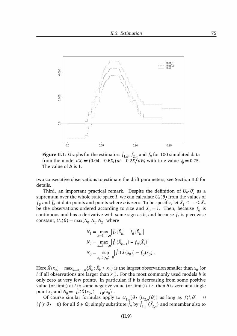
II.3. Estimation 75
0.0 0.05 0.10 0.15
0.0
0.00
50.
010
fhat_1fhat_2fhat
Figure II.1: Graphs for the estimators f1;n, f2;n and fn for 100 simulated data
from the model dXt = (0:040:6Xt)dt +0:2X γt dWt with true value γ0 = 0:75.
The value of ∆ is 1.
two consecutive observations to estimate the drift parameters, see Section II.6 fordetails.
Third, an important practical remark. Despite the definition of Un(θ) as asupremum over the whole state space I, we can calculate Un(θ) from the values offθ and fn at data points and points where b is zero. To be specific, let X1 Xn
be the observations ordered according to size and X0 = l. Then, because fθ is
continuous and has a derivative with same sign as b, and because fn is piecewiseconstant, Un(θ) = max(N0;N1;N2) where
N1 = maxk=1;::: ;n fn(Xk) fθ (Xk)
N2 = maxk=1;::: ;n fn(Xk1) fθ (Xk)
N0 = supx0:b(x0)=0
fnX(x0) fθ (x0):
Here X(x0) = maxk=0;::: ;nfXk : Xk x0g is the largest observation smaller than x0 (or
l if all observations are larger than x0). For the most commonly used models b isonly zero at very few points. In particular, if b is decreasing from some positivevalue (or limit) at l to some negative value (or limit) at r, then b is zero at a singlepoint x0 and N0 = fn(X(x0)) fθ (x0).
Of course similar formulas apply to U1;n(θ) (U2;n(θ)) as long as f (l;θ) = 0
( f (r;θ) = 0) for all θ 2 Θ; simply substitute fn by f1;n ( f2;n) and remember also to
(II.9)
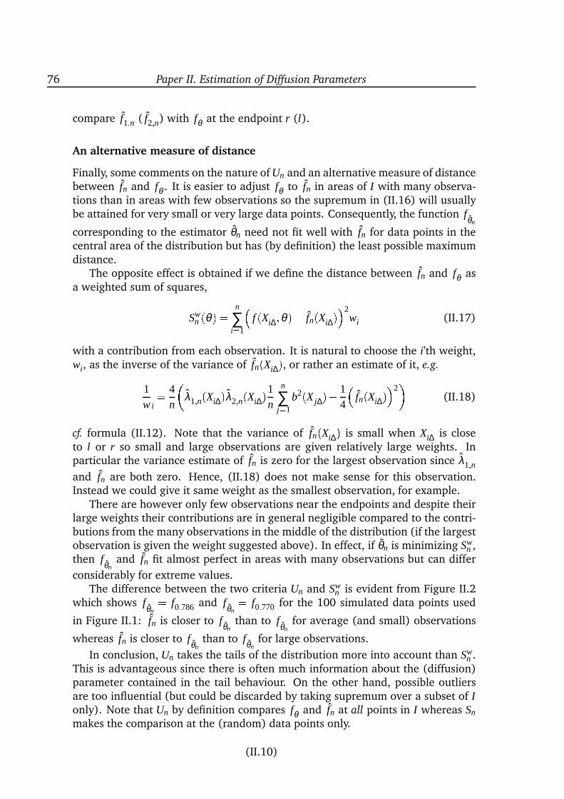
76 Paper II. Estimation of Diffusion Parameters
compare f1;n ( f2;n) with fθ at the endpoint r (l).
An alternative measure of distance
Finally, some comments on the nature of Un and an alternative measure of distancebetween fn and fθ . It is easier to adjust fθ to fn in areas of I with many observa-tions than in areas with few observations so the supremum in (II.16) will usuallybe attained for very small or very large data points. Consequently, the function fθn
corresponding to the estimator θn need not fit well with fn for data points in thecentral area of the distribution but has (by definition) the least possible maximumdistance.
The opposite effect is obtained if we define the distance between fn and fθ asa weighted sum of squares,
Swn (θ) = n
∑i=1
f (Xi∆;θ) fn(Xi∆)2
wi (II.17)
with a contribution from each observation. It is natural to choose the i’th weight,wi, as the inverse of the variance of fn(Xi∆), or rather an estimate of it, e.g.
1w i
= 4n
λ1;n(Xi∆)λ2;n(Xi∆)1
n
n
∑j=1
b2(X j∆) 14
fn(Xi∆)2
(II.18)
cf. formula (II.12). Note that the variance of fn(Xi∆) is small when Xi∆ is closeto l or r so small and large observations are given relatively large weights. Inparticular the variance estimate of fn is zero for the largest observation since λ1;nand fn are both zero. Hence, (II.18) does not make sense for this observation.Instead we could give it same weight as the smallest observation, for example.
There are however only few observations near the endpoints and despite theirlarge weights their contributions are in general negligible compared to the contri-butions from the many observations in the middle of the distribution (if the largestobservation is given the weight suggested above). In effect, if θn is minimizing Sw
n ,then fθn
and fn fit almost perfect in areas with many observations but can differ
considerably for extreme values.The difference between the two criteria Un and Sw
n is evident from Figure II.2which shows fθn
= f0:786 and fθn= f0:770 for the 100 simulated data points used
in Figure II.1: fn is closer to fθnthan to fθn
for average (and small) observations
whereas fn is closer to fθnthan to fθn
for large observations.
In conclusion, Un takes the tails of the distribution more into account than Swn .
This is advantageous since there is often much information about the (diffusion)parameter contained in the tail behaviour. On the other hand, possible outliersare too influential (but could be discarded by taking supremum over a subset of Ionly). Note that Un by definition compares fθ and fn at all points in I whereas Sn
makes the comparison at the (random) data points only.
(II.10)
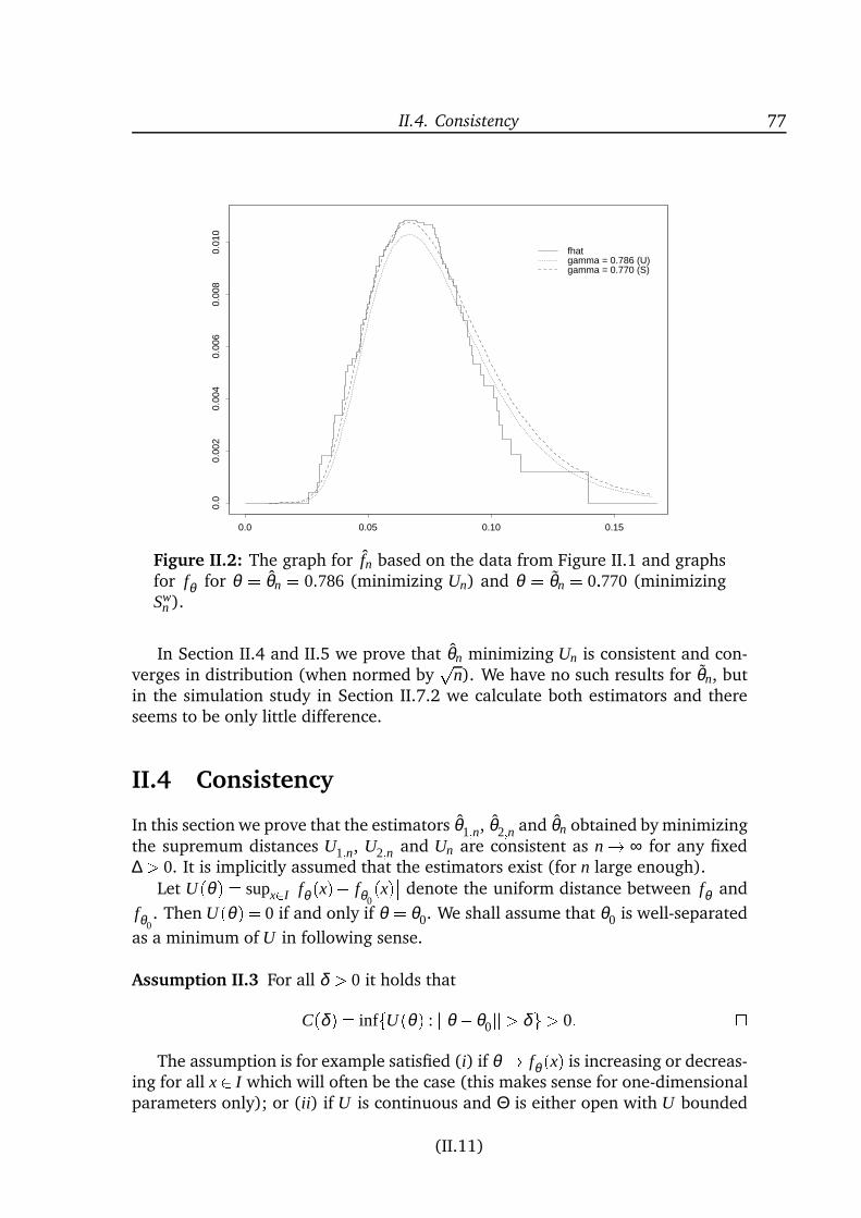
II.4. Consistency 77
0.0 0.05 0.10 0.15
0.0
0.00
20.
004
0.00
60.
008
0.01
0
fhatgamma = 0.786 (U)gamma = 0.770 (S)
Figure II.2: The graph for fn based on the data from Figure II.1 and graphsfor fθ for θ = θn = 0:786 (minimizing Un) and θ = θn = 0:770 (minimizingSw
n ).
In Section II.4 and II.5 we prove that θn minimizing Un is consistent and con-verges in distribution (when normed by
pn). We have no such results for θn, but
in the simulation study in Section II.7.2 we calculate both estimators and thereseems to be only little difference.
II.4 Consistency
In this section we prove that the estimators θ1;n, θ2;n and θn obtained by minimizingthe supremum distances U1;n, U2;n and Un are consistent as n ! ∞ for any fixed∆ > 0. It is implicitly assumed that the estimators exist (for n large enough).
Let U(θ) = supx2I
fθ (x) fθ0(x) denote the uniform distance between fθ and
fθ0. Then U(θ) = 0 if and only if θ = θ0. We shall assume that θ0 is well-separated
as a minimum of U in following sense.
Assumption II.3 For all δ > 0 it holds that
C(δ ) = inffU(θ) : jjθ θ0jj> δg> 0: The assumption is for example satisfied (i) if θ ! fθ (x) is increasing or decreas-
ing for all x 2 I which will often be the case (this makes sense for one-dimensionalparameters only); or (ii) if U is continuous and Θ is either open with U bounded
(II.11)
78 Paper II. Estimation of Diffusion Parameters
away from zero at the boundary or compact. A sufficient condition for continuityof U is that θ ! f (x;θ) is continuous, uniformly in x 2 I.
Theorem II.4 Assume that Assumptions II.1, II.2 and II.3 hold and that b changes
sign at most countably many times on I. If f (l;θ) = 0 ( f (r;θ) = 0) for all θ 2 Θthen θ1;n (θ2;n) is consistent for θ , and if f (l;θ) = f (r;θ) = 0 for all θ 2 Θ then θn is
consistent for θ as well.
Proof It follows from van der Vaart & Wellner (1996, Corollary 3.2.2) that it issufficient to show that the uniform distances converge in Pθ0
-probability (or almost
surely with respect to Pθ0) to U(θ), uniformly in θ .
First assume that f (l;θ) = 0 for all θ 2 Θ. By the triangle inequality for theuniform metric, it holds that jU1;n(θ)U(θ)j U1;n(θ0) for all θ 2 Θ so it sufficesto show
U1;n(θ0) = supx2I
f1;n(x) fθ0(x)! 0 (II.19)
Pθ0-almost surely. Note that pointwise convergence follows from the ergodic theo-
rem and Assumption II.2.We can write I =[ j2JI j where J is at most countable, each I j has the form [z1;z2
for some z1;z22 I or (l;z or [z;r) for some z2 I, and b is either non-positive or non-negative on I j. To prove (II.19) it is enough to show that supx2I j
f1;n(x) fθ0(x)!
0 for all j 2 J.Consider a j 2 J and assume for example that I j = [z1;z2 and that b 0 on I j.
Then fθ0and f1;n are non-decreasing on I j since (II.6) holds and f1;n is piecewise
constant with jump size b(Xk∆) at Xk∆.Since fθ0
is continuous it takes all values in [m;M where m = fθ0(z1) and M =
fθ0(z2). For K 2 N given we choose z1 = x0 < :: : < xK1 < xK = z2 such that fθ0
(xk) =m+ k(Mm)=K for all k = 0; : : : ;K. Then, for k = 0; : : : ;K1 and xk x xk+1,
f1;n(x) fθ0(x) f1;n(xk+1) fθ0
(xk)= f1;n(xk+1) fθ0(xk+1)+ fθ0
(xk+1) fθ0(xk)= f1;n(xk+1) fθ0
(xk+1)+(Mm)=K
since f1;n and fθ0are non-decreasing. Also
fθ0(x) f1;n(x) fθ0
(xk+1) f1;n(xk) fθ0(xk+1) fθ0
(xk)+ fθ0(xk) f1;n(xk)= fθ0
(xk) f1;n(xk)+(Mm)=K:Hence,
supx2I j
f1;n(x) fθ0(x) max
k=1;::: ;K f1;n(xk) fθ0(xk)+(Mm)=K:
(II.12)
II.5. Further asymptotic results 79
Now, choose A1; : : : ; AK such that Pθ0(Ak) = 1 and
f1;n(xk) fθ0(xk)! 0 on Ak for
all k = 1; : : : ;K. Then maxk=1;::: ;K f1;n(xk) fθ0(xk)! 0 on AK = A1\ AK and
supx2I j
f1;n(x) fθ0(x)! 0 on \∞
K=1AK, hence Pθ0-almost surely.
Similar arguments apply if I j = (l;z or I j = [x;r) and if b 0 on I j. We have nowproved (II.19) and thus uniform convergence of U1;n(θ) to U(θ) and consistency
of θ1;n. Consistency of θ2;n follows similarly if f (r;θ) = 0 for all θ 2 Θ.
Finally assume that f (l;θ)= f (r;θ)= 0 for all θ 2Θ. Recall that fn(x)= f1;n(x)2n λ2;n(x)∑n
i=1 b(Xi∆) and 0 λ2;n(x) 1. By the triangle inequality for the supremummetric, Un(θ)U(θ)j supx2I
fn(x) fθ0(x) supx2I
f1;n(x) fθ0(x)+2
1n
n
∑i=1
b(Xi∆)which converges uniformly in θ to zero Pθ0
-almost surely since Eθ0b(X0) = 0. This
proves consistency of θn. II.5 Further asymptotic results
In this section we show that θ1;n, θ2;n, and θn arep
n-consistent and furthermore
thatp
n(θn θ0) converges weakly as n ! ∞. For simplicity we only list the as-sumptions for a one-dimensional parameter but the convergence result holds formulti-dimensional parameters under similar conditions.
Consider first θi;n, i = 1;2. Proposition II.6 below claims that
Mi;n(h) = supx2I
n1=2 fi;n(x) fθ0+h=pn(x)converges weakly, uniformly in h 2 H for any compact set H R. Write Mi;n(h) =supx2I
M0i;n(x)M00
n (h;x) where
M0i;n(x) = n1=2 fi;n(x) fθ0
(x)M00
n (h;x) = n1=2 fθ0+h=pn(x) fθ0(x):
Note that the processes M00i;n and Mi;n are well-defined for n large enough provided
that θ0 is an inner point of Θ.
Recall that j fi;n(x)j 2n ∑n
j=1 jb(X j∆)j for all x2 I and that j fθ (x)j 2Eθ jb(X0)j for
all (x;θ) 2 IΘ. It follows that M00n takes values in l∞(H I) (since H is compact),
M0i;n in l∞(I), and thus Mi;n in l∞(H I). Here we have used the notation l∞(T ) for
the set of uniformly bounded, real functions on T; l∞(T ) = fg : supt2T jg(t)j< ∞g.The process M00
n is non-stochastic and M00n (h;x)! fθ0
(x)h pointwise if θ ! fθ (x)is differentiable in θ0 with derivative fθ0
(x). Assumption II.5.2 below ensures that
(II.13)
80 Paper II. Estimation of Diffusion Parameters
the convergence is suitably uniform. Note that it also ensures continuity of U in θ0,cf. the remark below Assumption II.3. A sufficient condition for Assumption II.5.2is that θ ! fθ (x) is twice differentiable in a neighbourhood Θ0 of θ0 for all x 2 Iwith the second derivative fθ (x) bounded in Θ0 I, i.e. sup(x;θ )2IΘ0
j fθ (x)j< ∞:For convergence of M0
n we will use empirical process theory (Arcones & Yu1994). See Appendix II.A for a brief introduction to the theory of empirical pro-cesses and the results used in the following. We assume that the drift has finiteabsolute p’th moment for some p > 2 (Assumption II.5.3) and that the temporaldependence in X decays fast enough. More precisely we assume that the β -mixingcoefficients decrease at an exponential rate (Assumption II.5.4). As usual for sta-tionary Markov processes, we define the β -mixing coefficients
βk = Zsup
A
pk∆;θ0(x;A)µθ0
(A)dµθ0(x)
where pk∆;θ0is the transition probability from time 0 to time k∆.
Assumption II.5 The true parameter value θ0 is an inner point of Θ and for anyx2 I the function θ ! fθ (x) = f (x;θ) is continuously differentiable in a neighbour-hood of θ0 with first partial derivative fθ = ∂ fθ=∂θ satisfying
1. fθ0is bounded, i.e. supx2I j fθ0
(x)j< ∞;
2. supx2I
fθ (x) fθ0(x)! 0 as θ ! θ0.
Furthermore,
3. Eθ0jb(X0)jp < ∞ for some p > 2;
4. there exist constants c1;c2 > 0 such that βk c1ec2k∆ for all k 1. Proposition II.6 Let H be an arbitrary compact subset of R, and assume that As-
sumptions II.1, II.2 and II.5 hold. Then fM1;n(h)gh2H converges weakly if f (l;θ) = 0for all θ 2Θ and fM2;n(h)gh2H converges weakly if f (r;θ) = 0 for all θ 2Θ.
Proof Assume first that f (l;θ) = 0 for all θ 2 Θ. We will use Theorem 2.1 fromArcones & Yu (1994) to show that fM0
1;n(x)gx2I converges weakly to a Gaussianprocess. By Assumption II.5.4 the required mixing condition is satisfied: with pfrom Assumption II.5.3. it holds that kp=(p2)(logk)2(p1)=(p2)βk ! 0 as k! ∞.
Define for x 2 I the function Fx : I ! R by Fx(y) = 2b(y)1fyxg and let F =fFxgx2I. Then, Eθ Fx(X0) = fθ (x) and by definition of f1;n,
M01;n(x) = n1=2
n
∑i=1
Fx(Xi∆)Eθ0
Fx(X0):(II.14)
II.5. Further asymptotic results 81
The function Fx(y) is jointly measurable in (x;y) and the envelope function of F ,supx2I jFxj= 2jbj, has finite p’th moment by Assumption II.5.3. Furthermore, it fol-
lows from Lemma II.11 in the appendix that F is a so-called Vapnik-Cervonenkissubgraph class of functions.
We conclude (Arcones & Yu 1994) that M01;n converges weakly in l∞(I) to a
tight, Gaussian process with Pθ0-almost all paths uniformly bounded and uniformly
continuous (with respect to the metric d on I given by d(x;y)2 = R (FxFy)2dµθ0).
Convergence of M00n follows from Assumption II.5.2, and the limit process M00
given by M00(h;x) = fθ0(x)h is in l∞(H I) by Assumption II.5.1. It now follows
from Slutsky’s Theorem that M01;nM00
n converges weakly in l∞(H I) and finally,convergence of M1;n in l∞(H) follows by the Continuous Mapping Theorem.
Similarly for M2;n if f (r;θ) = 0 for all θ 2 Θ. We have just established convergence of M1;n(h) and M2;n(h), uniformly in h2H
for compact sets H. Note however that the limit processes are not Gaussian (exceptperhaps for very special cases). In the much simpler case where the observationsare independent and identically uniformly distributed on (0;1) and b 1 (so thatf1;n(x) is simply the empirical distribution function) one has a — rather unpleasant
— expression for the distribution function of the limit M1(0) = supjM01(x)j, see
Billingsley (1968, Chapter 13). In the more complicated case under considerationin this paper it is not possible to identify the distribution of the limit.
By the above convergence results for Mi;n we can now showp
n-consistency of
θi;n, i = 1;2.
Theorem II.7 Assume that Assumptions II.1, II.2, II.3 and II.5 hold and furthermore
that fθ0(x0) 6= 0 for an x0 2 I. Then
pn(θ1;nθ0) is Op(1) if f (l;θ) = 0 for all θ 2Θ
andp
n(θ2;nθ0) is Op(1) if f (r;θ) = 0 for all θ 2 Θ.
Proof Recall that θi;n minimizes Ui;n(θ) = supx2I j fi;n(x) fθ (x)j and that Ui;n(θ)!U(θ) = supx2I j fθ0
(x) fθ (x)j Pθ0-almost surely as n ! ∞. It is easy to see thatp
nU(θi;n) is Op(1): By the triangle inequalitypnU(θi;n)pnUi;n(θi;n)+pnUi;n(θ0) 2
pnUi;n(θ0)
andp
nUi;n(θ0) = Mi;n(0) converges weakly and is hence Op(1).Recall the definition of C(δ ) from Assumption II.3 and note that P(pnjθi;n
θ0j> δ ) Pp
nU(θi;n)pnC(δ=pn) for all δ > 0. Hence, ifpnC(δ=pn)> cδ (II.20)
for all δ > 0, some constant c > 0 not depending on δ and n large enough, thenpnθi;nθ0
is Op(1).
(II.15)
82 Paper II. Estimation of Diffusion Parameters
To prove (II.20), choose c;η > 0 such that U(θ)> cjθ θ0j for all θ with jθ θ0j η. This is possible by differentiability of θ ! fθ (x0) (use e.g. c = j fθ0
(x0)j=2).
For n > δ 2=η2,
C(δ=pn) = inf
U(θ) : jθ θ0j> δ=pn= min
inf
U(θ) : δ=pn < jθ θ0j η; inf
U(θ) : jθ θ0j> η
= min
inf
U(θ) : δ=pn < jθ θ0j η;C(η):
Now, C(η) > 0 by Assumption II.3 and inf
U(θ) : δ=pn < jθ θ0j < η! 0 as
n! ∞ since U(θ0) = 0 and U is continuous in θ0. Hence, for n large enough
C(δ=pn) = inf
U(θ) : δ=pn < jθ θ0j< η> cδ=pn
which proves (II.20) and thusp
n-consistency of θi;n. We now consider the situation where f (l;θ) = f (r;θ) = 0 for all θ and show
thatp
nθnθ0
is Op(1) and even converges weakly.
Define M0n(x) = n1=2
fn(x) fθ0
(x) and Mn(h) = supx2I jM0n(x)M00
n (h;x)j. We
first give a uniform convergence result for Mn. As in the proof of proposition II.6we use empirical process theory to show convergence of M0. In this case it ishowever not immediate that the relevant class of functions is a Vapnik-Cervonenkissubgraph class, and rather than showing that it is (which is indeed the case, seeLemma II.12 in the appendix), we choose to work with covering numbers directly.
Proposition II.8 Assume that Assumptions II.1, II.2 and II.5 hold and that f (l;θ) =f (r;θ) = 0 for all θ 2 Θ. Then fMn(h)gh2H converges weakly for any compact set
H R.
Proof Recall that fn = λ1;n f1;n + λ2;n f2;n where λ j;n converges pointwise (and uni-formly as we shall argue below) Pθ0
-almost surely to λ j := λθ0; j, j = 1;2. We first
argue that it suffices to consider λ1 f1;n +λ2 f2;n instead of fn: By adding and sub-
tracting λ1 f1;n and λ2 f2;n we get
fn = λ1;nλ1
f1;n + λ2;nλ2
f2;n +λ1 f1;n +λ2 f2;n= λ1;nλ1
f1;n fθ0
+ λ2;nλ2
f2;n fθ0
+λ1 f1;n +λ2 f2;nand hence,
M0n = λ1;nλ1
M0
1;n + λ2;nλ2
M0
2;n +M0λ ;n (II.21)
where M0λ ;n(x) = n1=2
λ1(x) f1;n(x)+λ2(x) f2;n(x) fθ0
(x):Since λ1 is continuous and decreasing from one to zero, it takes all values
in the unit interval (0;1). From arguments almost identical to those leading to
(II.16)
II.5. Further asymptotic results 83
the uniform convergence (II.19) of f1;n to fθ0, it follows that λ1;n(x)! λ1(x) and
hence also λ2;n(x)! λ2(x) Pθ0-almost surely, uniformly in x 2 I. In the proof of
Proposition II.6 we showed that M01;n and M0
2;n converge weakly and it now follows
from Slutsky’s Theorem that M0n converges in l∞(I) if M0
λ ;n does.
Now, let F = fFxgx2I where Fx : I ! R is defined by
Fx(y) = 2λ1(x)b(y)1fyxg2λ2(x)b(y)1fy>xg= 2b(y)λ1(x)1fy>xg; y 2 I:Then Eθ Fx(X0) = fθ (x) and M0
λ ;n(x) = n1=2 ∑ni=1
Fx(Xi∆) fθ0
(x). The function
Fx(y) is jointly measurable in (x;y) and the envelope function supx2I jFxj = 2jbj ofF has finite p’th moment by Assumption II.5.3.
Let Q be a probability measure on I with b2 L2(Q), let jj jjQ be the L2(Q)-norm
and define BQ = Rb2dQ. We show that the jj jjQ-covering number N(ε;F ; jj jjQ),
which is the minimal number of jj jjQ-balls of radius ε needed to cover F , is at
most 32BQ=ε2 (at least for small ε).
First, note that for all x;z 2 IjjFxFzjj2Q = Z (FxFz)2dQ= 4Z
b2λ1(x)1(x;r)λ1(z)+1(z;r)2dQ 8
Zb2λ1(x)λ1(z)2 dQ+8
Zb21(x;r)1(z;r)2 dQ:
Define BQ(x) = R xl b2dQ = R
b21(l;xdQ and use the notation ^ for minimum and _for maximum. Then,
1(x;r)1(z;r)2 = 1(l;x_z1(l;x^z andjjFxFzjj2Q 8
λ1(x)λ1(z)2BQ +8BQ(x_ z)8BQ(x^ z):
Next, for 0< ε < 4B1=2Q
given, let K = 16BQ=ε2 (or rather the smallest integer
larger than this number). The functions λ1 and BQ are continuous, λ1 decreases
from 1 to 0 and BQ increases from 0 to BQ so we can choose u1; : : : ;uK1 andv1; : : : ;vK1 such that
8BQλ1(uk) = 8BQ(vk) = kε2=2; k = 1; : : : ;K1:For k = 2; : : : ;2K 1, define yk as the (k 1)’st smallest of the 2(K 1) pointsfuk;vkgk=1;::: ;K1. Also, let y1 = l and y2K = r. Then jjFxFzjjQ < ε for x;z2 [yk;yk+1for some k = 1; : : : ;2K1. Indeed, let yk x z yk+1 and let u = maxfu j yk; j =1; : : : ;K1g and u = minfu j yk; j = 1; : : : ;K1g be the u j ’s that are closest to yk
(II.17)
84 Paper II. Estimation of Diffusion Parameters
(and smaller/larger respectively). Define v and v similarly. Then,jjFzFzjj2Q 8λ1(x)λ1(z)2BQ +8BQ(z)8BQ(x) 8λ1(u)λ1(u)2BQ +8BQ(v)8BQ(v) ε2=22
8BQ+ ε2=2< ε2;
and F can be covered by 2K balls (with respect to jj jjQ) of radius ε. Hence,
N(ε;F ; jj jjQ) 2K = 32BQ=ε2 = 32jjbjj2L2(Q)=ε2 (II.22)
for any Q with b 2 L2(Q) (and ε small enough). In particular (II.22) holds for
Q = µθ0and hence
R ∞0
logN(ε;F ; jj jjµθ0
)1=2dε < ∞:
It follows (Arcones & Yu 1994, Lemma 2.1) that M0λ ;n converges in l∞(I) and
hence from (II.21) that M0n converges in l∞(I). Finally, weak convergence of M00
nand Mn follows as in the proof of Proposition II.6. Theorem II.9 Assume that Assumptions II.1, II.2, II.3, and II.5 hold and f (l;θ) =f (r;θ) = 0 for all θ 2Θ. If, in addition, fθ0
(x0) 6= 0 for some x02 I thenp
n(θnθ0) is
Op(1) and if furthermore fθ0(x) 6= 0 for all x 2 I, then
pn(θnθ0) converges weakly.
Proof Thep
n-consistency follows exactly as in the proof of Theorem II.7.For the weak convergence it then suffices to show that Pθ0
-almost all paths of
the limit M of Mn has a unique minimum (van der Vaart & Wellner 1996, Theorem3.2.2).
The limit process fM(h)gh2R has the form M(h) = supx2I jM0(x) fθ0(x)hj where
M0 is the Gaussian limit of M0n. We first show that M0(x)! 0 Pθ0
-almost surely as
x& l and x% r, that is Pθ0(M0 2 A) = 1 where A = fϕ = (ϕx)x2I 2 l∞(I) : limx&l ϕx =
limx%r ϕx = 0g.It is easy to see that A is closed with respect to the uniform metric d(ϕ;ϕ 0) =
supx2I jϕxϕ 0xj. Indeed, let (ϕn) be a sequence from A with ϕn ! ϕ and let ε > 0.Choose N such that d(ϕn;ϕ)< ε=2 for all n N. In addition, choose xl and xr suchthat
ϕNx
< ε=2 for x xl and for x xr. Then, for x xl and x xr,jϕxj jϕxϕNx j+ ϕN
x
supx2I
ϕxϕNx
+ ϕNx
< ε
so ϕ 2 A and A is closed.For every n 1 all paths of M0
n are in A since fn(x) = 0 for all x < minfXi∆ : i =1; : : : ;ng and all x maxfXi∆ : i = 1; : : : ;ng and limx!l fθ0
(x) = limx!r fθ0(x) = 0. It
now follows from Portmanteau’s theorem that Pθ0(M0 2 A) limsupn!∞ Pθ0
(M0n 2
A) = 1.
(II.18)
II.5. Further asymptotic results 85
Now, all paths h ! M(h) satisfy M(h)! ∞ as h ! ∞ since M(h) M0(x)fθ0
(x)h and fθ0(x) 6= 0 for any fixed x2 I (for this it suffices that fθ0
(x0)= 0 for some
x0 2 I). All paths are continuous since jM(h2)M(h1)j jh2h1jsupx2I j fθ0(x)j for
all h1;h2 2 R and hence have a minimum. We must show that the minimum isunique.
It is easy to see that all paths of M are (weakly) convex: for h1;h2 2 R andα 2 (0;1)
Mαh1+(1α)h2
= supx2I
αM0(x) fθ0(x)h1
+(1α)M0(x) fθ0(x)h2
α supx2I
M0(x) fθ0(x)h1
+(1α)supx2I
M0(x) fθ0(x)h2
= αM(h1)+(1α)M(h2):It holds Pθ0
-almost surely that M0 is continuous and belongs to the set A from
above. Consider a path h!M(h) for which this is the case and assume that h1 < h2both minimize M. Let m = M(h1) = M(h2) be the minimum value. By convexityM(h) = m where h = (h1+h2)=2 is the mid point between h1 and h2.
By definition, M(h) = supx2I
M0(x) fθ0(x)h. Choose a sequence (xn) from I
such thatM0(xn) fθ0
(xn)h m1=n for each n 1. For j = 1;2 and all n 1,
m = M(h j) M0(xn) fθ0(xn)h j
implying that
fθ0(xn)(h2h1)=2 1=n and hence
fθ0(xn)! 0 as n! ∞.
Since fθ0(x) 6= 0 for all x 2 I it thus holds for any l < x1 < x2 < r that xn 62 [x1;x2
for n large enough and hence M0(xn)! 0 as n! ∞. It follows that
m = M(h) = limn!∞
M0(xn) fθ0(xn)h= 0 (II.23)
so M(h1) = M(h2) = m = 0. This is not possible, though, since for any x 2 I at leastone of the values jM0(x) fθ0
(x)h1j and jM0(x) fθ0(x)h2j is strictly positive.
We conclude that M has a unique minimum Pθ0-almost surely and hence thatp
nθnθ0
converges weakly.
We have just shown that θn converges weakly, but there is no reason to believethat the limit distribution is Gaussian. Simulation studies indicate however thatthe limit distribution might be close to normal.
Parts of the above proof could be repeated with M1 or M2 substituted for M. Ifh and (xn) are as above with M replaced by M1, say, then it would still hold thatxn could be made arbitrarily close to l or r by choosing n large enough. But M0
1(x)does not converge to zero as x ! r so limn!∞
M01(xn) fθ0
(xn)h, corresponding
to (II.23), need not be zero and cannot be rejected as the minimum value of M1.
(II.19)
86 Paper II. Estimation of Diffusion Parameters
Similarly, M02(x) does not converge to zero as x & l and we cannot rule out the
possibility that M1 and M2 have several minimum points.
Note that the limits of M01(x) and M0
2(x) as x tends to l and r do exist withlimx%r M0
1(x) and limx&l M02(x) Gaussian and limx&l M0
1(x) = limx%r M02(x) = 0 Pθ0
-
almost surely. This can be proved via Portmanteau’s theorem and the continuousmapping theorem.
Finally, a comment on Assumption II.5: The boundedness conditions may seemrather restrictive but in practice we can take a supremum over a (very large) com-pact subset of I rather than over I when forming the criterion functions U1;n, U2;nand Un. Then, by continuity, the boundedness conditions are automatically satis-fied.
II.6 When the drift is not known
So far, we have assumed that the drift is completely known which is of courseunrealistic. When this is not the case we follow the approach of Aït-Sahalia (1996)in that we suggest estimating the drift beforehand and then simply pretend thatthe drift is equal to its estimator when estimating the diffusion parameters.
More precisely we assume that the drift has a parametric specification b(x) =b(x;ξ ) and that the parameter ξ can be estimated consistently without any knowl-edge of the diffusion parameter θ . This is the case if b is linear and the martingalepart of X is a genuine martingale: then we can use martingale estimation func-tions as suggested by Bibby & Sørensen (1995). Let ξ be the estimator of ξ andredefine f1;n in the obvious way
f1;n(x) = 2n
n
∑i=1
b(Xi∆; ξ )1fXi∆xg:
Similarly for f2;n and fn. The true function f of course also depends on ξ . Again
we just plug in the estimator and minimize supx2(l;r) f (x; ξ ;θ) fn(x):II.7 Examples
We now consider two particular models, namely the Ornstein-Uhlenbeck process(or Vasicek model) and the CKLS model. Of course, for the Ornstein-Uhlenbeckprocess the estimation problem is already solved since the transition probabilitiesare known and we can do maximum likelihood estimation. We study it brieflyanyway since we get some qualitative results on the improvement caused by usingfn rather than f1;n or f2;n. For the CKLS model we discuss various estimationmethods and compare them to our estimation approach in a simulation study.
(II.20)
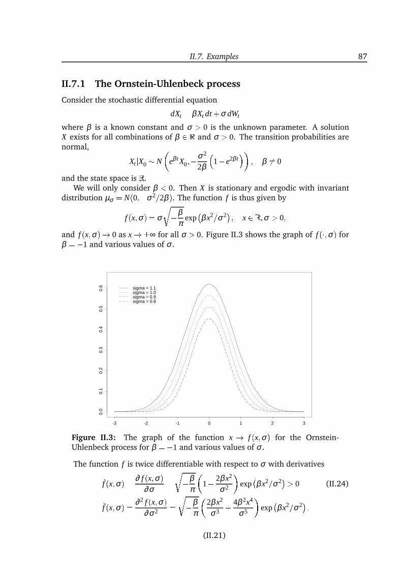
II.7. Examples 87
II.7.1 The Ornstein-Uhlenbeck process
Consider the stochastic differential equation
dXt = βXt dt +σ dWt
where β is a known constant and σ > 0 is the unknown parameter. A solutionX exists for all combinations of β 2 R and σ > 0. The transition probabilities arenormal,
XtjX0 N
eβ tX0;σ2
2β
1 e2β t
; β 6= 0
and the state space is R.We will only consider β < 0. Then X is stationary and ergodic with invariant
distribution µσ = N(0;σ2=2β ). The function f is thus given by
f (x;σ) = σrβ
πexpβx2=σ2 ; x 2 R;σ > 0;
and f (x;σ)! 0 as x!∞ for all σ > 0. Figure II.3 shows the graph of f (;σ) forβ =1 and various values of σ .
-3 -2 -1 0 1 2 3
0.0
0.1
0.2
0.3
0.4
0.5
0.6 sigma = 1.1
sigma = 1.0sigma = 0.9sigma = 0.8
Figure II.3: The graph of the function x ! f (x;σ) for the Ornstein-Uhlenbeck process for β =1 and various values of σ .
The function f is twice differentiable with respect to σ with derivatives
f (x;σ) = ∂ f (x;σ)∂σ
=rβπ
1 2βx2
σ2
expβx2=σ2> 0 (II.24)
f (x;σ) = ∂ 2 f (x;σ)∂σ2 =rβ
π
2βx2
σ3 + 4β 2x4
σ5
expβx2=σ2 :
(II.21)
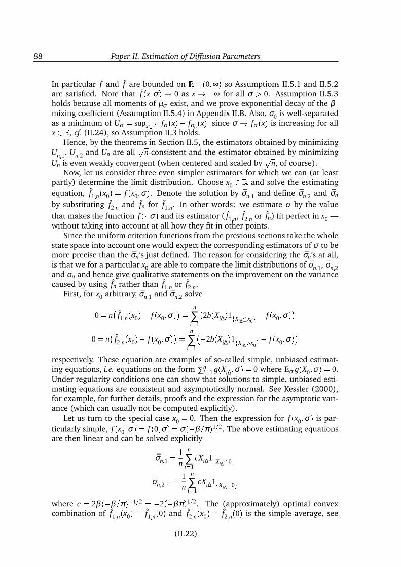
88 Paper II. Estimation of Diffusion Parameters
In particular f and f are bounded on R (0;∞) so Assumptions II.5.1 and II.5.2are satisfied. Note that f (x;σ)! 0 as x !∞ for all σ > 0. Assumption II.5.3holds because all moments of µσ exist, and we prove exponential decay of the β -mixing coefficient (Assumption II.5.4) in Appendix II.B. Also, σ0 is well-separatedas a minimum of Uσ = supx2R j fσ (x) fσ0
(x)j since σ ! fσ (x) is increasing for allx 2 R, cf. (II.24), so Assumption II.3 holds.
Hence, by the theorems in Section II.5, the estimators obtained by minimizingUn;1, Un;2 and Un are all
pn-consistent and the estimator obtained by minimizing
Un is even weakly convergent (when centered and scaled byp
n, of course).Now, let us consider three even simpler estimators for which we can (at least
partly) determine the limit distribution. Choose x0 2 R and solve the estimating
equation, f1;n(x0) = f (x0;σ). Denote the solution by σn;1 and define σn;2 and σn
by substituting f2;n and fn for f1;n. In other words: we estimate σ by the value
that makes the function f (;σ) and its estimator ( f1;n, f2;n or fn) fit perfect in x0 —without taking into account at all how they fit in other points.
Since the uniform criterion functions from the previous sections take the wholestate space into account one would expect the corresponding estimators of σ to bemore precise than the σn’s just defined. The reason for considering the σn’s at all,is that we for a particular x0 are able to compare the limit distributions of σn;1, σn;2and σn and hence give qualitative statements on the improvement on the variancecaused by using fn rather than f1;n or f2;n.
First, for x0 arbitrary, σn;1 and σn;2 solve
0= n
f1;n(x0) f (x0;σ)= n
∑i=1
2b(Xi∆)1fXi∆x0g f (x0;σ)
0= n
f2;n(x0) f (x0;σ)= n
∑i=1
2b(Xi∆)1fXi∆>x0g f (x0;σ)respectively. These equation are examples of so-called simple, unbiased estimat-ing equations, i.e. equations on the form ∑n
i=1g(Xi∆;σ) = 0 where Eσ g(X0;σ) = 0.Under regularity conditions one can show that solutions to simple, unbiased esti-mating equations are consistent and asymptotically normal. See Kessler (2000),for example, for further details, proofs and the expression for the asymptotic vari-ance (which can usually not be computed explicitly).
Let us turn to the special case x0 = 0. Then the expression for f (x0;σ) is par-
ticularly simple, f (x0;σ) = f (0;σ) = σ(β=π)1=2. The above estimating equationsare then linear and can be solved explicitly
σn;1 = 1n
n
∑i=1
cXi∆1fXi∆0gσn;2 =1
n
n
∑i=1
cXi∆1fXi∆>0gwhere c = 2β (β=π)1=2 = 2(βπ)1=2. The (approximately) optimal convexcombination of f1;n(x0) = f1;n(0) and f2;n(x0) = f2;n(0) is the simple average, see
(II.22)
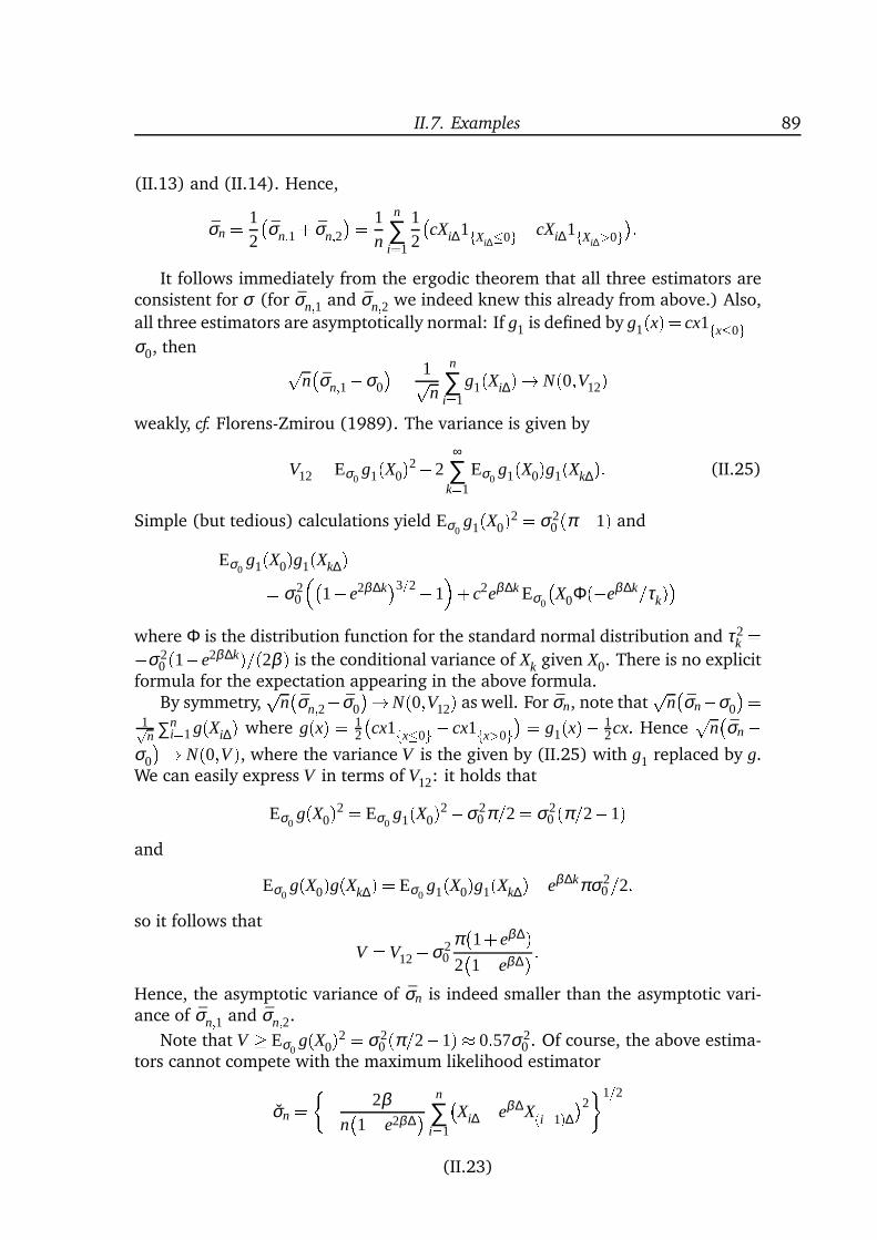
II.7. Examples 89
(II.13) and (II.14). Hence,
σn = 12
σn;1+ σn;2= 1
n
n
∑i=1
12
cXi∆1fXi∆0g cXi∆1fXi∆>0g:
It follows immediately from the ergodic theorem that all three estimators areconsistent for σ (for σn;1 and σn;2 we indeed knew this already from above.) Also,
all three estimators are asymptotically normal: If g1 is defined by g1(x)= cx1fx0gσ0, then p
nσn;1σ0
= 1pn
n
∑i=1
g1(Xi∆)! N(0;V12)weakly, cf. Florens-Zmirou (1989). The variance is given by
V12 = Eσ0g1(X0)2+2
∞
∑k=1
Eσ0g1(X0)g1(Xk∆): (II.25)
Simple (but tedious) calculations yield Eσ0g1(X0)2 = σ2
0(π1) and
Eσ0g1(X0)g1(Xk∆)= σ2
0
1 e2β∆k3=21
+ c2eβ∆k Eσ0
X0Φ(eβ∆k=τk)
where Φ is the distribution function for the standard normal distribution and τ2k =σ2
0(1e2β∆k)=(2β ) is the conditional variance of Xk given X0. There is no explicitformula for the expectation appearing in the above formula.
By symmetry,p
nσn;2σ0
!N(0;V12) as well. For σn, note thatp
nσnσ0
=1pn ∑n
i=1g(Xi∆) where g(x) = 12
cx1fx0g cx1fx>0g = g1(x) 1
2cx: Hencep
nσn
σ0
! N(0;V ), where the variance V is the given by (II.25) with g1 replaced by g.We can easily express V in terms of V12: it holds that
Eσ0g(X0)2 = Eσ0
g1(X0)2σ20π=2= σ2
0(π=21)and
Eσ0g(X0)g(Xk∆) = Eσ0
g1(X0)g1(Xk∆) eβ∆kπσ20=2:
so it follows that
V =V12σ20
π1+ eβ∆)
21 eβ∆) :
Hence, the asymptotic variance of σn is indeed smaller than the asymptotic vari-ance of σn;1 and σn;2.
Note that V Eσ0g(X0)2 = σ2
0(π=21) 0:57σ20 . Of course, the above estima-
tors cannot compete with the maximum likelihood estimator
σn = 2βn1 e2β∆
n
∑i=1
Xi∆ eβ∆X(i1)∆2
1=2
(II.23)
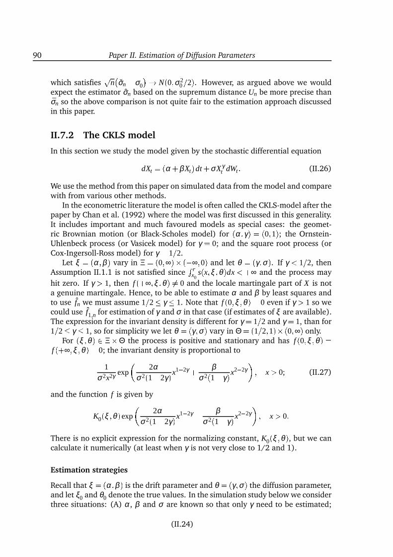
90 Paper II. Estimation of Diffusion Parameters
which satisfiesp
nσnσ0
! N(0;σ20=2). However, as argued above we would
expect the estimator σn based on the supremum distance Un be more precise thanσn so the above comparison is not quite fair to the estimation approach discussedin this paper.
II.7.2 The CKLS model
In this section we study the model given by the stochastic differential equation
dXt = (α +βXt)dt +σX γt dWt : (II.26)
We use the method from this paper on simulated data from the model and comparewith from various other methods.
In the econometric literature the model is often called the CKLS-model after thepaper by Chan et al. (1992) where the model was first discussed in this generality.It includes important and much favoured models as special cases: the geomet-ric Brownian motion (or Black-Scholes model) for (α;γ) = (0;1); the Ornstein-Uhlenbeck process (or Vasicek model) for γ = 0; and the square root process (orCox-Ingersoll-Ross model) for γ = 1=2.
Let ξ = (α;β ) vary in Ξ = (0;∞) (∞;0) and let θ = (γ;σ). If γ < 1=2, thenAssumption II.1.1 is not satisfied since
R rx0
s(x;ξ ;θ)dx < +∞ and the process may
hit zero. If γ > 1, then f (+∞;ξ ;θ) 6= 0 and the locale martingale part of X is nota genuine martingale. Hence, to be able to estimate α and β by least squares andto use fn we must assume 1=2 γ 1. Note that f (0;ξ ;θ) = 0 even if γ > 1 so wecould use f1;n for estimation of γ and σ in that case (if estimates of ξ are available).The expression for the invariant density is different for γ = 1=2 and γ = 1, than for1=2 γ 1, so for simplicity we let θ = (γ;σ) vary in Θ = (1=2;1) (0;∞) only.
For (ξ ;θ) 2 ΞΘ the process is positive and stationary and has f (0;ξ ;θ) =f (+∞;ξ ;θ) = 0; the invariant density is proportional to
1σ2x2γ exp
2α
σ2(12γ)x12γ + βσ2(1 γ)x22γ
; x > 0; (II.27)
and the function f is given by
K0(ξ ;θ)exp
2α
σ2(12γ)x12γ + βσ2(1 γ)x22γ
; x > 0:There is no explicit expression for the normalizing constant, K0(ξ ;θ), but we cancalculate it numerically (at least when γ is not very close to 1/2 and 1).
Estimation strategies
Recall that ξ = (α;β ) is the drift parameter and θ = (γ;σ) the diffusion parameter,and let ξ0 and θ0 denote the true values. In the simulation study below we considerthree situations: (A) α, β and σ are known so that only γ need to be estimated;
(II.24)
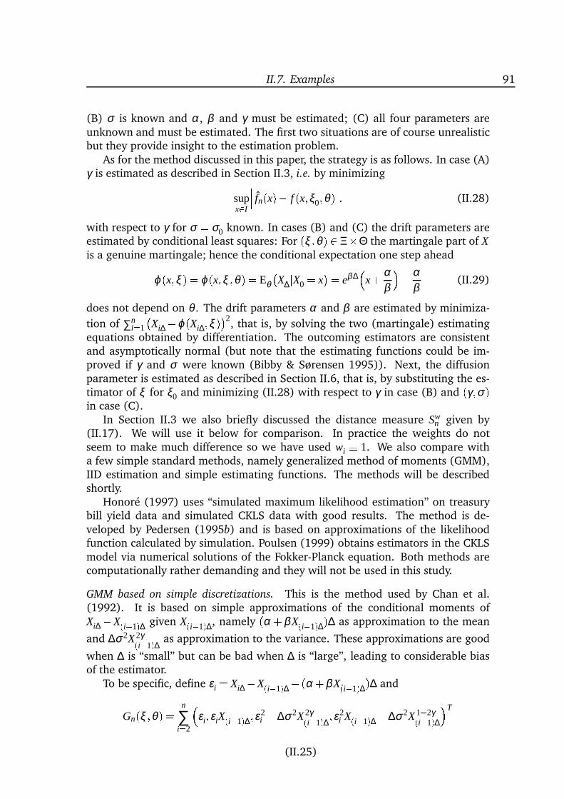
II.7. Examples 91
(B) σ is known and α, β and γ must be estimated; (C) all four parameters areunknown and must be estimated. The first two situations are of course unrealisticbut they provide insight to the estimation problem.
As for the method discussed in this paper, the strategy is as follows. In case (A)γ is estimated as described in Section II.3, i.e. by minimizing
supx2I
fn(x) f (x;ξ0;θ): (II.28)
with respect to γ for σ = σ0 known. In cases (B) and (C) the drift parameters areestimated by conditional least squares: For (ξ ;θ) 2 ΞΘ the martingale part of Xis a genuine martingale; hence the conditional expectation one step ahead
ϕ(x;ξ ) = ϕ(x;ξ ;θ) = EθX∆jX0 = x
= eβ∆
x+ αβ
αβ
(II.29)
does not depend on θ . The drift parameters α and β are estimated by minimiza-
tion of ∑ni=1
Xi∆ϕ(Xi∆;ξ )2, that is, by solving the two (martingale) estimating
equations obtained by differentiation. The outcoming estimators are consistentand asymptotically normal (but note that the estimating functions could be im-proved if γ and σ were known (Bibby & Sørensen 1995)). Next, the diffusionparameter is estimated as described in Section II.6, that is, by substituting the es-timator of ξ for ξ0 and minimizing (II.28) with respect to γ in case (B) and (γ;σ)in case (C).
In Section II.3 we also briefly discussed the distance measure Swn given by
(II.17). We will use it below for comparison. In practice the weights do notseem to make much difference so we have used wi 1. We also compare witha few simple standard methods, namely generalized method of moments (GMM),IID estimation and simple estimating functions. The methods will be describedshortly.
Honoré (1997) uses “simulated maximum likelihood estimation” on treasurybill yield data and simulated CKLS data with good results. The method is de-veloped by Pedersen (1995b) and is based on approximations of the likelihoodfunction calculated by simulation. Poulsen (1999) obtains estimators in the CKLSmodel via numerical solutions of the Fokker-Planck equation. Both methods arecomputationally rather demanding and they will not be used in this study.
GMM based on simple discretizations. This is the method used by Chan et al.(1992). It is based on simple approximations of the conditional moments ofXi∆X(i1)∆ given X(i1)∆, namely (α +βX(i1)∆)∆ as approximation to the mean
and ∆σ2X2γ(i1)∆ as approximation to the variance. These approximations are good
when ∆ is “small” but can be bad when ∆ is “large”, leading to considerable biasof the estimator.
To be specific, define εi = Xi∆X(i1)∆ (α +βX(i1)∆)∆ and
Gn(ξ ;θ) = n
∑i=2
εi;εiX(i1)∆;ε2
i ∆σ2X2γ(i1)∆;ε2i X(i1)∆∆σ2X1+2γ(i1)∆T
(II.25)
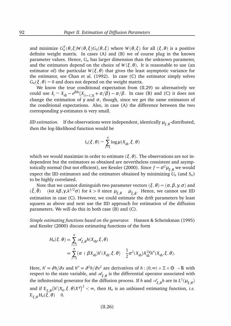
92 Paper II. Estimation of Diffusion Parameters
and minimize GTn (θ ;ξ )W (θ ;ξ )Gn(θ ;ξ ) where W (θ ;ξ ) for all (ξ ;θ) is a positive
definite weight matrix. In cases (A) and (B) we of course plug in the knownparameter values. Hence, Gn has larger dimension than the unknown parameter,and the estimators depend on the choice of W (ξ ;θ). It is reasonable to use (anestimator of) the particular W (ξ ;θ) that gives the least asymptotic variance forthe estimator, see Chan et al. (1992). In case (C) the estimator simply solvesGn(ξ ;θ) = 0 and does not depend on the weight matrix.
We know the true conditional expectation from (II.29) so alternatively wecould use εi = Xi∆ eβ∆X(i1)∆ + α=β
+ α=β . In case (B) and (C) it does not
change the estimation of γ and σ , though, since we get the same estimators ofthe conditional expectations. Also, in case (A) the difference between the twocorresponding γ-estimates is very small.
IID estimation. If the observations were independent, identically µξ ;θ -distributed,
then the log-likelihood function would be
ln(ξ ;θ) = n
∑i=1
logµ(Xi∆;ξ ;θ)which we would maximize in order to estimate (ξ ;θ). The observations are not in-dependent but the estimators so obtained are nevertheless consistent and asymp-totically normal (but not efficient), see Kessler (2000). Since f = σ2µξ ;θ we would
expect the IID estimators and the estimators obtained by minimizing Un (and Sn)to be highly correlated.
Note that we cannot distinguish two parameter vectors (ξ ;θ) = (α;β ;γ;σ) and(ξ ; θ) = (kα;kβ ;γ;k1=2σ) for k > 0 since µξ ;θ = µξ ;θ . Hence, we cannot use IID
estimation in case (C). However, we could estimate the drift parameters by leastsquares as above and next use the IID approach for estimation of the diffusionparameters. We will do this in both case (B) and (C).
Simple estimating functions based on the generator. Hansen & Scheinkman (1995)and Kessler (2000) discuss estimating functions of the form
Hn(ξ ;θ) = n
∑i=1Aξ ;θ h(Xi∆;ξ ;θ)= n
∑i=1
(α +βXi∆)h0(Xi∆;ξ ;θ)+ 12
σ2(Xi∆)X2γi∆ h00(Xi∆;ξ ;θ):
Here, h0 = ∂h=∂x and h00 = ∂ 2h=∂x2 are derivatives of h : (0;∞)ΞΘ ! R withrespect to the state variable, and Aξ ;θ is the differential operator associated with
the infinitesimal generator for the diffusion process. If h and Aξ ;θ h are in L1(µξ ;θ )and if Eξ ;θh0(X0;ξ ;θ)X γ2 < ∞, then Hn is an unbiased estimating function, i.e.
Eξ ;θ Hn(ξ ;θ) = 0.
(II.26)
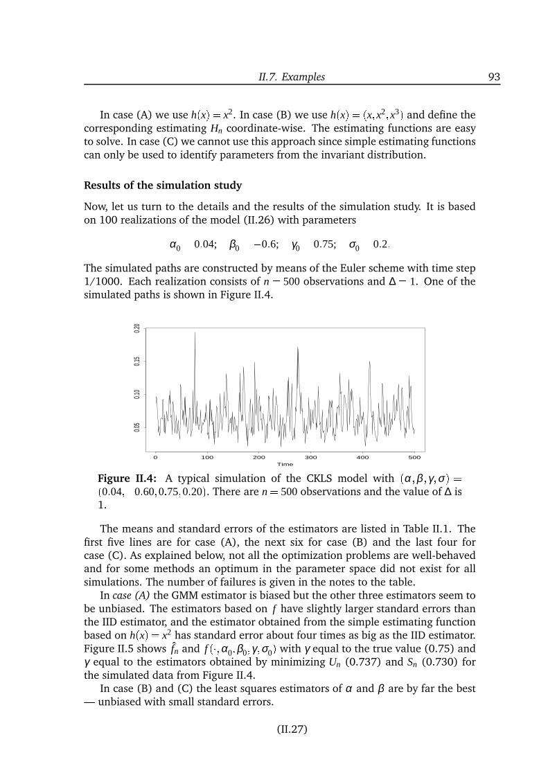
II.7. Examples 93
In case (A) we use h(x) = x2. In case (B) we use h(x) = (x;x2;x3) and define thecorresponding estimating Hn coordinate-wise. The estimating functions are easyto solve. In case (C) we cannot use this approach since simple estimating functionscan only be used to identify parameters from the invariant distribution.
Results of the simulation study
Now, let us turn to the details and the results of the simulation study. It is basedon 100 realizations of the model (II.26) with parameters
α0 = 0:04; β0 =0:6; γ0 = 0:75; σ0 = 0:2:The simulated paths are constructed by means of the Euler scheme with time step1/1000. Each realization consists of n = 500 observations and ∆ = 1. One of thesimulated paths is shown in Figure II.4.
Time
0 100 200 300 400 500
0.05
0.10
0.15
0.20
Figure II.4: A typical simulation of the CKLS model with (α;β ;γ;σ) =(0:04;0:60;0:75;0:20). There are n = 500observations and the value of ∆ is1.
The means and standard errors of the estimators are listed in Table II.1. Thefirst five lines are for case (A), the next six for case (B) and the last four forcase (C). As explained below, not all the optimization problems are well-behavedand for some methods an optimum in the parameter space did not exist for allsimulations. The number of failures is given in the notes to the table.
In case (A) the GMM estimator is biased but the other three estimators seem tobe unbiased. The estimators based on f have slightly larger standard errors thanthe IID estimator, and the estimator obtained from the simple estimating functionbased on h(x) = x2 has standard error about four times as big as the IID estimator.Figure II.5 shows fn and f (;α0;β0;γ;σ0) with γ equal to the true value (0.75) andγ equal to the estimators obtained by minimizing Un (0.737) and Sn (0.730) forthe simulated data from Figure II.4.
In case (B) and (C) the least squares estimators of α and β are by far the best— unbiased with small standard errors.
(II.27)
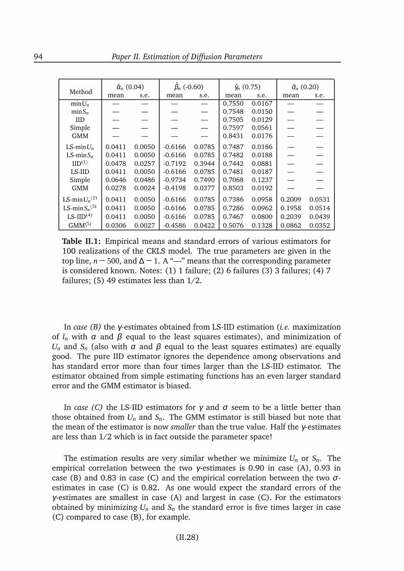
94 Paper II. Estimation of Diffusion Parameters
Methodαn (0.04) βn (-0.60) γn (0.75) σn (0.20)
mean s.e. mean s.e. mean s.e. mean s.e.minUn — — — — 0.7550 0.0167 — —minSn — — — — 0.7548 0.0150 — —
IID — — — — 0.7505 0.0129 — —Simple — — — — 0.7597 0.0561 — —GMM — — — — 0.8431 0.0176 — —
LS-minUn 0.0411 0.0050 -0.6166 0.0785 0.7487 0.0186 — —LS-minSn 0.0411 0.0050 -0.6166 0.0785 0.7482 0.0188 — —
IID(1) 0.0478 0.0257 -0.7192 0.3944 0.7442 0.0881 — —LS-IID 0.0411 0.0050 -0.6166 0.0785 0.7481 0.0187 — —Simple 0.0646 0.0486 -0.9734 0.7490 0.7068 0.1237 — —GMM 0.0278 0.0024 -0.4198 0.0377 0.8503 0.0192 — —
LS-minUn(2) 0.0411 0.0050 -0.6166 0.0785 0.7386 0.0958 0.2009 0.0531
LS-minSn(3) 0.0411 0.0050 -0.6166 0.0785 0.7286 0.0962 0.1958 0.0514
LS-IID(4) 0.0411 0.0050 -0.6166 0.0785 0.7467 0.0800 0.2039 0.0439
GMM(5) 0.0306 0.0027 -0.4586 0.0422 0.5076 0.1328 0.0862 0.0352
Table II.1: Empirical means and standard errors of various estimators for100 realizations of the CKLS model. The true parameters are given in thetop line, n = 500, and ∆ = 1. A “—” means that the corresponding parameteris considered known. Notes: (1) 1 failure; (2) 6 failures (3) 3 failures; (4) 7failures; (5) 49 estimates less than 1/2.
In case (B) the γ-estimates obtained from LS-IID estimation (i.e. maximizationof ln with α and β equal to the least squares estimates), and minimization ofUn and Sn (also with α and β equal to the least squares estimates) are equallygood. The pure IID estimator ignores the dependence among observations andhas standard error more than four times larger than the LS-IID estimator. Theestimator obtained from simple estimating functions has an even larger standarderror and the GMM estimator is biased.
In case (C) the LS-IID estimators for γ and σ seem to be a little better thanthose obtained from Un and Sn. The GMM estimator is still biased but note thatthe mean of the estimator is now smaller than the true value. Half the γ-estimatesare less than 1/2 which is in fact outside the parameter space!
The estimation results are very similar whether we minimize Un or Sn. Theempirical correlation between the two γ-estimates is 0.90 in case (A), 0.93 incase (B) and 0.83 in case (C) and the empirical correlation between the two σ -estimates in case (C) is 0.82. As one would expect the standard errors of theγ-estimates are smallest in case (A) and largest in case (C). For the estimatorsobtained by minimizing Un and Sn the standard error is five times larger in case(C) compared to case (B), for example.
(II.28)
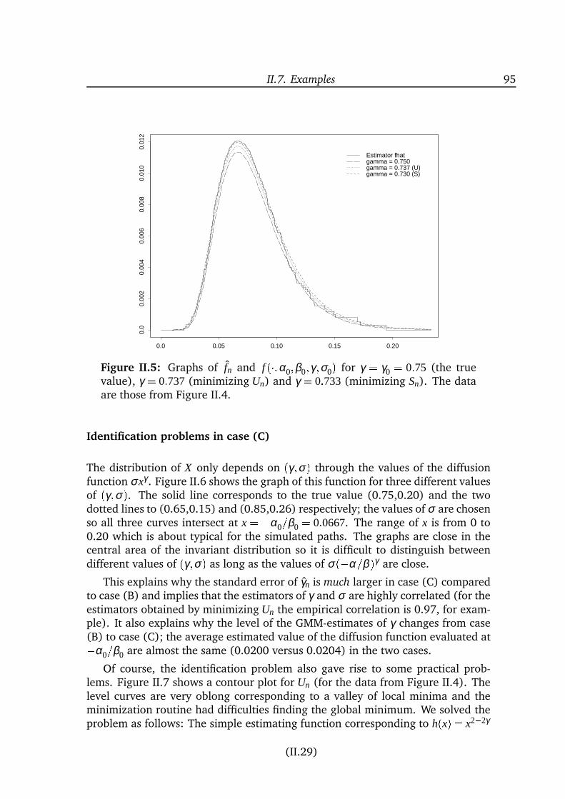
II.7. Examples 95
0.0 0.05 0.10 0.15 0.20
0.0
0.00
20.
004
0.00
60.
008
0.01
00.
012
Estimator fhatgamma = 0.750gamma = 0.737 (U)gamma = 0.730 (S)
Figure II.5: Graphs of fn and f (;α0;β0;γ;σ0) for γ = γ0 = 0:75 (the truevalue), γ = 0:737 (minimizing Un) and γ = 0:733 (minimizing Sn). The dataare those from Figure II.4.
Identification problems in case (C)
The distribution of X only depends on (γ;σ) through the values of the diffusionfunction σxγ . Figure II.6 shows the graph of this function for three different valuesof (γ;σ). The solid line corresponds to the true value (0.75,0.20) and the twodotted lines to (0.65,0.15) and (0.85,0.26) respectively; the values of σ are chosenso all three curves intersect at x = α0=β0 = 0:0667. The range of x is from 0 to0.20 which is about typical for the simulated paths. The graphs are close in thecentral area of the invariant distribution so it is difficult to distinguish betweendifferent values of (γ;σ) as long as the values of σ(α=β )γ are close.
This explains why the standard error of γn is much larger in case (C) comparedto case (B) and implies that the estimators of γ and σ are highly correlated (for theestimators obtained by minimizing Un the empirical correlation is 0.97, for exam-ple). It also explains why the level of the GMM-estimates of γ changes from case(B) to case (C); the average estimated value of the diffusion function evaluated atα0=β0 are almost the same (0.0200 versus 0.0204) in the two cases.
Of course, the identification problem also gave rise to some practical prob-lems. Figure II.7 shows a contour plot for Un (for the data from Figure II.4). Thelevel curves are very oblong corresponding to a valley of local minima and theminimization routine had difficulties finding the global minimum. We solved theproblem as follows: The simple estimating function corresponding to h(x) = x22γ
(II.29)
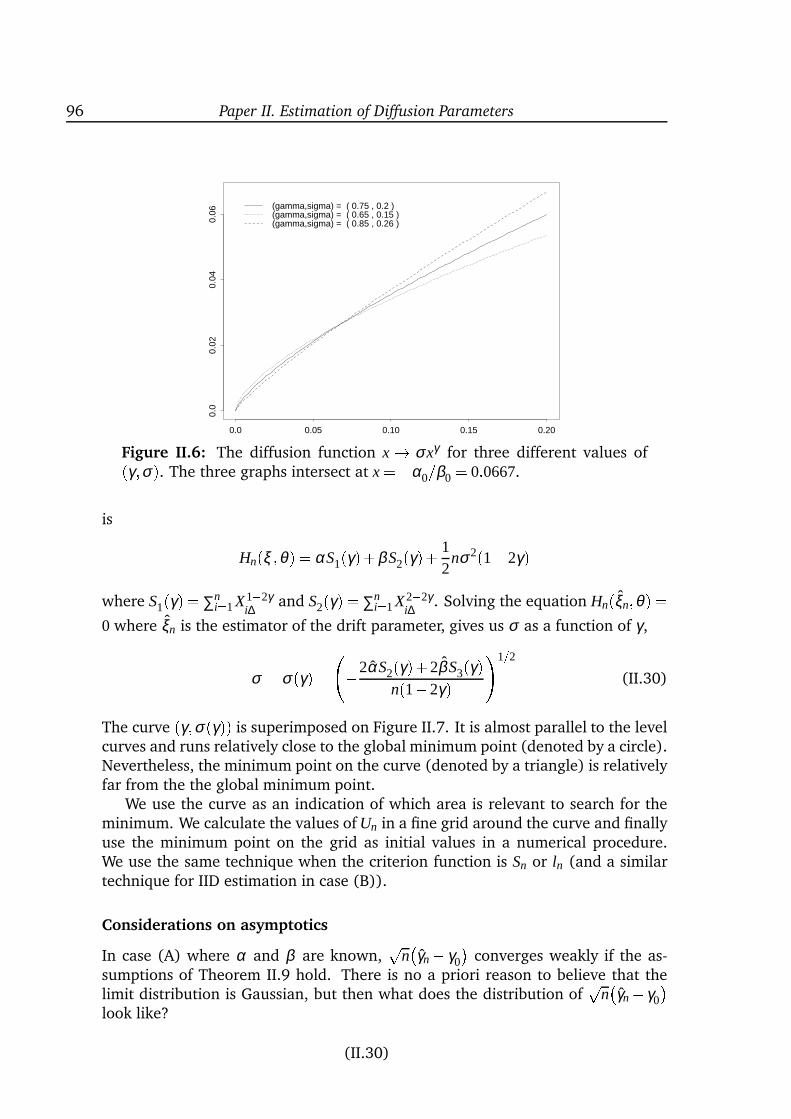
96 Paper II. Estimation of Diffusion Parameters
0.0 0.05 0.10 0.15 0.20
0.0
0.02
0.04
0.06
(gamma,sigma) = ( 0.75 , 0.2 )(gamma,sigma) = ( 0.65 , 0.15 )(gamma,sigma) = ( 0.85 , 0.26 )
Figure II.6: The diffusion function x ! σxγ for three different values of(γ;σ). The three graphs intersect at x =α0=β0 = 0:0667.
is
Hn(ξ ;θ) = αS1(γ)+βS2(γ)+ 12
nσ2(12γ)where S1(γ) = ∑n
i=1X12γi∆ and S2(γ) = ∑n
i=1X22γi∆ . Solving the equation Hn(ξn;θ) =
0 where ξn is the estimator of the drift parameter, gives us σ as a function of γ,
σ = σ(γ) = 2αS2(γ)+2βS3(γ)n(12γ) !1=2
(II.30)
The curve (γ;σ(γ)) is superimposed on Figure II.7. It is almost parallel to the levelcurves and runs relatively close to the global minimum point (denoted by a circle).Nevertheless, the minimum point on the curve (denoted by a triangle) is relativelyfar from the the global minimum point.
We use the curve as an indication of which area is relevant to search for theminimum. We calculate the values of Un in a fine grid around the curve and finallyuse the minimum point on the grid as initial values in a numerical procedure.We use the same technique when the criterion function is Sn or ln (and a similartechnique for IID estimation in case (B)).
Considerations on asymptotics
In case (A) where α and β are known,p
nγn γ0
converges weakly if the as-
sumptions of Theorem II.9 hold. There is no a priori reason to believe that thelimit distribution is Gaussian, but then what does the distribution of
pnγn γ0
look like?
(II.30)
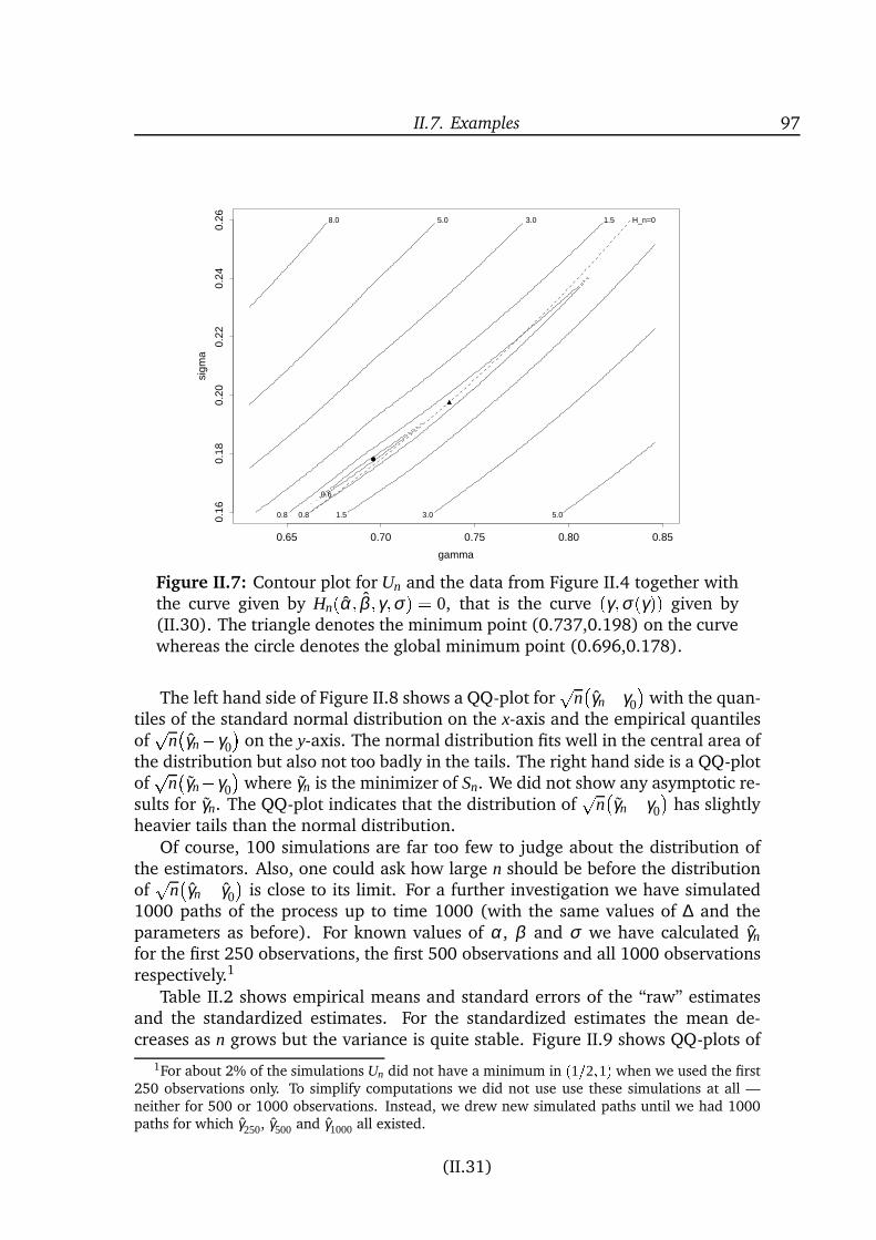
II.7. Examples 97
gamma
sigm
a
0.65 0.70 0.75 0.80 0.85
0.16
0.18
0.20
0.22
0.24
0.26
0.6
0.80.8
1.5
1.5 3.0
3.0
5.0
5.08.0 H_n=0
Figure II.7: Contour plot for Un and the data from Figure II.4 together withthe curve given by Hn(α; β ;γ;σ) = 0, that is the curve (γ;σ(γ)) given by(II.30). The triangle denotes the minimum point (0.737,0.198) on the curvewhereas the circle denotes the global minimum point (0.696,0.178).
The left hand side of Figure II.8 shows a QQ-plot forp
nγnγ0
with the quan-
tiles of the standard normal distribution on the x-axis and the empirical quantilesofp
nγnγ0
on the y-axis. The normal distribution fits well in the central area of
the distribution but also not too badly in the tails. The right hand side is a QQ-plotofp
nγnγ0
where γn is the minimizer of Sn. We did not show any asymptotic re-
sults for γn. The QQ-plot indicates that the distribution ofp
nγn γ0
has slightly
heavier tails than the normal distribution.Of course, 100 simulations are far too few to judge about the distribution of
the estimators. Also, one could ask how large n should be before the distributionofp
nγn γ0
is close to its limit. For a further investigation we have simulated
1000 paths of the process up to time 1000 (with the same values of ∆ and theparameters as before). For known values of α, β and σ we have calculated γn
for the first 250 observations, the first 500 observations and all 1000 observationsrespectively.1
Table II.2 shows empirical means and standard errors of the “raw” estimatesand the standardized estimates. For the standardized estimates the mean de-creases as n grows but the variance is quite stable. Figure II.9 shows QQ-plots of
1For about 2% of the simulations Un did not have a minimum in (1=2;1) when we used the first250 observations only. To simplify computations we did not use use these simulations at all —neither for 500 or 1000 observations. Instead, we drew new simulated paths until we had 1000paths for which γ250, γ500 and γ1000 all existed.
(II.31)
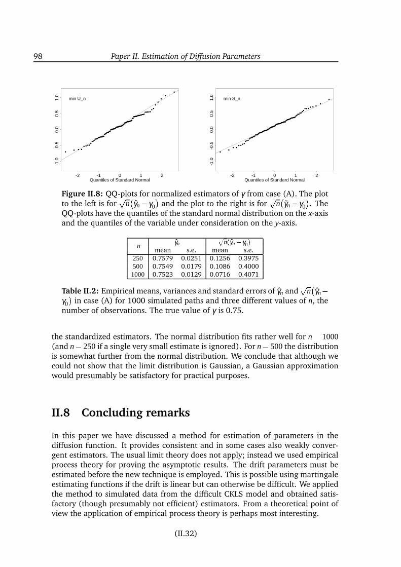
98 Paper II. Estimation of Diffusion Parameters
••
•••
• •
•
••
• ••
••
•
•
•
•
•
•
•
•
•
•
••
• ••
•
•
••••
•
••
•••
•
•
•
•
•
•
•
•
•
••
•
•
•
•
••
•
•
••
•
•
•
•
•
••
•
•
•
•
•
••
•
•
•
•
••
• •
••
•• •
•
••
•
•
•
•
•
•
•
Quantiles of Standard Normal-2 -1 0 1 2
-1.0
-0.5
0.0
0.5
1.0
min U_n
•
••
••
••
•
•
• •
••
••
•
•
•
•
•
•
•
•
•
••
•
••
••
•
•
• • •
•
•
•
••
•
•
•
•
•
•
•
•
•
•
••
•
•
•
•
••
•
•
•• • ••
•
•
•
•
•
•
••
••
•
•
•
•
•
••
•
•
•••• •
•
••
•
•
•
•
•
•
•
Quantiles of Standard Normal-2 -1 0 1 2
-1.0
-0.5
0.0
0.5
1.0
min S_n
Figure II.8: QQ-plots for normalized estimators of γ from case (A). The plotto the left is for
pnγn γ0
and the plot to the right is for
pnγn γ0
. The
QQ-plots have the quantiles of the standard normal distribution on the x-axisand the quantiles of the variable under consideration on the y-axis.
nγn
pn(γn γ0)
mean s.e. mean s.e.250 0.7579 0.0251 0.1256 0.3975500 0.7549 0.0179 0.1086 0.40001000 0.7523 0.0129 0.0716 0.4071
Table II.2: Empirical means, variances and standard errors of γn andp
nγn
γ0
in case (A) for 1000 simulated paths and three different values of n, the
number of observations. The true value of γ is 0.75.
the standardized estimators. The normal distribution fits rather well for n = 1000(and n= 250if a single very small estimate is ignored). For n= 500the distributionis somewhat further from the normal distribution. We conclude that although wecould not show that the limit distribution is Gaussian, a Gaussian approximationwould presumably be satisfactory for practical purposes.
II.8 Concluding remarks
In this paper we have discussed a method for estimation of parameters in thediffusion function. It provides consistent and in some cases also weakly conver-gent estimators. The usual limit theory does not apply; instead we used empiricalprocess theory for proving the asymptotic results. The drift parameters must beestimated before the new technique is employed. This is possible using martingaleestimating functions if the drift is linear but can otherwise be difficult. We appliedthe method to simulated data from the difficult CKLS model and obtained satis-factory (though presumably not efficient) estimators. From a theoretical point ofview the application of empirical process theory is perhaps most interesting.
(II.32)
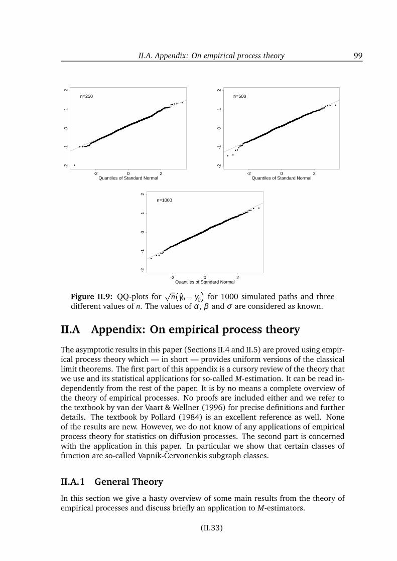
II.A. Appendix: On empirical process theory 99
•
•• •••
•
••
•
•
•••
•
••
•
••
• •
•
••
•
•
•
•
•
•
•
•
•
•
• •
•••
•
•
•
••
••
•••
••
•
• ••
•
••
••
•
•
•
•••
••
••
•
•
••
•
•
••
• •
•
•
•
•
••••
•
•
••
•
•• ••
•
•
•
•
•
•
•••
•
••
•
••
•
•
•
••
••
••
•
•
•••
•
• •
••
•
••
••
•
•
••
•• ••
••
•• •
•
••
•
••
•
•
•
•
•
•
•
•
•••
•
••
•
•
••
••
•
•
•
•
••
•
•
•
•
•
•
•
••
••
•
•
•
•
•
••• • •
•
•
• ••
•••
•• •
•••• •
•
•
•
•••
• ••
•
••
•
•
••
•
••
••
•
••
••
••
•
•••
•
••
••
•
•
•
••
••••• •
•
•••
•
••
•
•••• •••
•
•
••
•
•
••
•
•
••
•
••
•
•
•
••
••
•
••
•
• ••
•••
•
•••
•
•••
•
•
•
••
•
•••
•
••
•
•
•
•
•
•
•
••
•
• ••
•
•
•
•
•
•
•
••
•
•
•
••
••
•
••
••
•
•
•••
•
•
••
•
•
•••
• •
•
•
•
••
•••
•
•
••
••
•
•
•
•
••
•
••
•
•
•
••••
•
••
•
••
•
•
••
•
•
•••
•• •
•
••
•
••
•
•
• ••
••
••
••
•
••
•
••
••
•
•
••
•••
•
•
•
•
•
•••
• ••
••• •
•
•
•
•
••
• •
• •
•
••
•
••
•
•
•
••
• ••
•
•
••
•
••
••••
•
••
•
•
••
•
••
•
•
••
••
• •
••
••
•
•
•
••
•
•
•
•• •••
•
••
••
•••
••
••
•
•
••
•
••
•••
•
• ••
•
• • •
•
•
••
•
•
•
••
•
•
••
•
•
•
•
•
•
•
•••
••
••
•• •
••
•
••
•••
•
••
••• •
•
•
••
•
•
••
•
•••
••
••
••
•
•
•
•
•
•
•
••
••• ••
•
•
••
•
••
•••
••
••
•
•
••
••••
•
• •
•
••
•••
••
• • ••
•
•• •••
•
••
•
••
•
•
•• •
•
• •
• •
•
•••
••
•
••
••
••
•
•
•
•
•
••
••
•
••
••
•• •
•
•
•
••
•••
••
•••
•
•••
•
••
•
•
• ••
•
•
••
•
• ••
•
••
•
••
• ••
••
••
•••
•
•
••
•
• ••
••
•••
••
•
••
•
•
••
••
•
•••
•
•
•
•• •
•• •
•
•
•
••
•
•
•
•
•
•
•
•
•
••
•••
••
•
•••
• • •••
•
•
•
•
•
• ••
• •
•
• •
•• •
•
••
• •
•
••
••
•
•
••
•
••
••
•••
••
•
•••
••
••
• ••
•
• ••
•
•
•
•• •
•
••
•
•
•
••• •
•
•
••
••
•
•
••
•
••••
•
••
•
••
••
•
•
••
•
•• •
•
•
•
•
••
•
••
•• •
•
••
•
••
•
•
•••
•
••
•
•••
••
••
•
•
•
Quantiles of Standard Normal-2 0 2
-2-1
01
2
n=250
•
•
•
••
•
••
•
•
•
•
•
••
•
••
••
•
•
•
•
••
•
•
•
••
•
•
•
••
•
•
•
•••
••
••
•
••
•
•
•
•
•• •
•
••••
••
•
•
••
••
••
••
••
•
•
•
•
• •
••
•
•
•
•••
•• ••
••
• ••
•
•
•
•
•• •••
• ••
••
•
••
•
•
•
•
•
•
•
•
•
•
•••
•
•
••
•
••
•
•
•
••
•
••
••
•
• •
•• ••
•
•
••
•
•
•
•
•
•
•
•
••
•
•
•
•
••
•
•
•
••
•
•
••
•
••
•
•
•
•••
•
••
•
••
•
•
•
•
•
• • •
•
••
••
••
•••• •
••
•
•
•
••
••
•••
•
••
••
•
•
•
• •
• •
•
••
••
••
••
•
•
•••
•
•••
• •••
• ••
•
•
••
••
•
••
•• ••
••••
•
•••
•
••
•
••
• •• ••
•
••
•
• •
•
• ••
•
••
•• •
••••
••
••
• •
••
•
••••
••
••
•
•
•
•
•
•
••
•
••••
•
• •• •
•
•••
•• •
•
••
••
•
•••
•
••
•
•
••
••
•
••
•••
•
••
•
•
•
••
•
••
•
•
•
•
••
•
••
••••
•
•
•
• ••
••
• •••
•
•••
•
•
•
•••
•••
•
••
•
•
••
•
•
•
••
•
••
••
•
••
•
••
• •
•
•
••
• ••
••
•
•
••
•
•••••
•
•
•
••
•
••
•••
•••
••
•
••
•
••
••
•••
•
••••
•••••
••
•
•
• •
•
•••
•
•
••
•
•
•
•• •• •
•
•
••
•
•
••
•
•
•
•
••
•
•••
••
• ••
•••
•
•
••
• •
•
•
•
•
•
••
•
••
• •
••••
•
•
••
••
•
•• ••
•••
•
•
•
•
• ••
•
• ••
•• ••
••
••
•••
•
••
•
•
•
•
•
•
•• ••
•
• •
•
••
•
•
••
• •
•
•
•
•
••••
••
••
•
••
•
•••••
• •••
•
•
•
•
• • •
•
••
••
•
•
•
•
••
••
•••
•
•
•
• ••••
•
• ••
•
•
•
•
•
••••
••
•
••
••
•
•
•
•
•
•
•••
•
•
•
•
•••
•
•
•
•
• ••
•••
•
•
••
••• •••
•
•
•
•• ••
•
•
•
••
••
••
• •
••••
••
••
••
•
•
•
••
•
•
•
•
••
•
•
•
• •
•
•• •
•
••
• •
•
••
••
••
• •••
•
•
••
••••
••
•
•
•••
•
•
•
•
•
••
•
••
•
•
••
•
•
••
••
•
•
•
•
••
•
•••
• •
•
•
•••
••
••••
••
•••
••
•
•
•
••
••
••
•
•
• •
••
•
•
••
•
••
••
• •• •••
••
••
• ••
•
••
••
•
•
•
••
•
••
•
••
••
•
••
• ••
•••
••
••
•
•
•
•
•
•
•
•
•
••
•
•
•
••
•
••
•• •
•
•
•
•
••
•
•
•
•
••
•
••
•
•
••
••
•
•
•
•
Quantiles of Standard Normal-2 0 2
-2-1
01
2
n=500
•
•
•
•
••
• •
••
•
•• •
••
•
•
••
• ••
••
•••
•
•
••
•
•
•
••
••
••
•••
•
•
•
•
•••
•
••
• •
•
•
•
• ••
•
•
•
•
••
••
••
•
•
•
•
•
•
••
•
•
• •
•
••
•
•••
•
• •
•
•
•
•
•
•
•
•
•
••
••
•
•
••
••
••
•
•
•
•••
•
•
•••
•
•
••
•
•••
•
•
••
••
•
•• •
••
••••
••
•
•
•
• •
••
•
•
••
•
•
•
••
••
•
•
••
•
•• •
•
• •
•
• ••
•
•
•••
•
••
•
••
• •
•
•
•
• •••
•• •
••
•
••
•
•
••
•
•
•
••
•••••
••
•
•
••
•
•
•
••
•••
•
•
••
••
•
••
•
••
••
••
•
•
•
•
•
• ••
••
•••
••
•
••
• • •
•• •
•
•
••
••
••
••
••
•
•
•
•
•
•
•
•
•
•
••
••
•
•••
••
•••••
••
• ••
••
•
•
••
• •
•
••
••
•
•
•
•
•
•
•
•
•
• ••
•
•
•
•••
•
••••
•••
•••
••
•
••
••
•
• •
•
•
•
•
••
••
••• •
•
•••
•••
••
••
••
••
••
•
• ••
•
•
•
•
•
•
•
•••
•
•
•• •
•
•
•
••
•
•
•
•
•
•
•
••
•
•
•
•
••••
••
• • •
••
•
••
•
•
•
• ••
••
•
•
•
•
••
•
• ••• •
•
•
•
•
••
••
•
•••
•••
•
•
•
• ••
•
•
•
•
••
••
•
••
•
•
••
• ••
•
• •
•••
•
•
• •
•
•
•
•
••
•••
•
••
••
•
• •
•
•
••
•
•
•
•••
•••
•
••
••
••
•
• ••
••
•
•
•
•
•
•
•
•
• •
•
• ••
•• •
••
•
• •
•••• •
•
••
•
••
•
•
••
•
••
••
•
•
•
••
•
•• ••
•
•
•
••
•
•
•• •
••
•
•
••
••
•
•
•
••
••
•
•
•
•••
••
•• ••• •
•
••
•
•
•
•••
•
••
•
•••
•
••
••
••
•
••
•
••
••
•
••
••
••
•
••
•
••
••
••
•
••
•••
• ••
•
••
• •
•
•
••
•
•
•
•••
•
•
••••
•
•
•
•••
••
•
•
•
••
•• •
•
•
•
•
•
•
•
••
•
•
•
•
•
•
••
•
••
•
•
•
••
•
•
•••
••
••
•
••
•
•
• ••
•
•
•
• ••
••
••
•
••
•
•
•••
•
•
•
•
••
•
•
•
•
•
•
• •••
•
•
•
••••
••
•
•
•• •
••
••
••
•
••
•
•
•
•
•
•
•
•
••
••
••
••
•
••
•
•
••
•
••
•••
•••
•
•
••
•
•
••
•
••
•
•
•• • •
••
•
•
••
•
• •
•
•
••••
•
•
•
•
•
•
•
••
•
••
•
••
•
•
•
••
•
•
•
••
••
•
• •
•••
•
• •
•
• •
••
••
•
•
•
•
• •••
•••
•
• •••
••
•
•
•
•
• ••
•
••
••
•
•
•• •
••
•
•• ••
Quantiles of Standard Normal-2 0 2
-2-1
01
2
n=1000
Figure II.9: QQ-plots forp
nγn γ0
for 1000 simulated paths and three
different values of n. The values of α, β and σ are considered as known.
II.A Appendix: On empirical process theory
The asymptotic results in this paper (Sections II.4 and II.5) are proved using empir-ical process theory which — in short — provides uniform versions of the classicallimit theorems. The first part of this appendix is a cursory review of the theory thatwe use and its statistical applications for so-called M-estimation. It can be read in-dependently from the rest of the paper. It is by no means a complete overview ofthe theory of empirical processes. No proofs are included either and we refer tothe textbook by van der Vaart & Wellner (1996) for precise definitions and furtherdetails. The textbook by Pollard (1984) is an excellent reference as well. Noneof the results are new. However, we do not know of any applications of empiricalprocess theory for statistics on diffusion processes. The second part is concernedwith the application in this paper. In particular we show that certain classes offunction are so-called Vapnik-Cervonenkis subgraph classes.
II.A.1 General Theory
In this section we give a hasty overview of some main results from the theory ofempirical processes and discuss briefly an application to M-estimators.
(II.33)
100 Paper II. Estimation of Diffusion Parameters
Glivenko-Cantelli and Donsker classes
First of all, we point out what is meant by uniform limit theorems. Let Z;Z1;Z2; : : :be independent, identically distributed random variables defined on some proba-bility space (E;E ;Pr) with values in Z (equipped with some σ -algebra) and com-mon distribution P = Z(Pr). Furthermore, let f : Z ! R be measurable. Then,according to the classical law of large numbers, the average of f (Z1); : : : ; f (Zn)converges, that is
1n
n
∑i=1
f (Zi)! E f (Z) (II.31)
almost surely and in L1 provided that f 2 L1(P). The classical central limit theoremasserts that the centered and scaled sum converges weakly to a normal distribu-tion, that is
1pn
n
∑i=1
f (Zi)E f (Z)! N
0;E f (Z)E f (Z)2
(II.32)
weakly provided that f 2 L2(P) with E f 2(Z)> 0.The corresponding uniform theorems claim that (II.31) and (II.32) hold uni-
formly for f varying in suitably small classesF . To be specific, the uniform versionof the law of large numbers states that
supf2F 1n n
∑i=1
f (Zi)E f (Z)! 0 (II.33)
almost surely, and F is called a Glivenko-Cantelli class if (II.33) holds.To define a uniform central limit theorem, assume that supf2F f (z)E f (Z)<
∞ for all z 2 Z and let l∞(F ) be the set of functionals G : F ! R for whichsupf2F jG( f )j< ∞. Equip l∞(F) with the uniform topology. Then, for each n, the
functional Gn :F ! R defined by
f !Gn( f ) = 1pn
n
∑i=1
f (Zi)E f (Z) (II.34)
is an element of l∞(F ) and one can ask whether Gn converges weakly to a Gaus-sian limit G 2 l∞(F ). The process Gn is called the empirical process indexed by Fand F is called a Donsker class if Gn converges weakly in l∞(F ).Covering numbers, entropy and VC classes
Now, when is a certain class a Glivenko-Cantelli or Donsker class? Informally, onehas to measure the size of the class and decide whether it is small enough for theconvergence results hold for all f 2F simultaneously.
Covering and entropy numbers are very important in this context. For a givennorm jj jj on F and ε > 0 the covering number N(ε;F ; jj jj) is defined as the
(II.34)
II.A. Appendix: On empirical process theory 101
minimal number of jj jj-balls of radius ε needed to cover F . The logarithm of thecovering number is called the entropy. Obviously, if G F (and the same normis used on both F and G ) then N(ε;G ; jj jj) N(ε;F ; jj jj). Hence, the coveringnumber (or entropy number) makes sense as a measure of size of a given class.
Note that N(ε;F ; jj jj) is one for large ε if supf ;g2F jj f gjj<∞. Also, N(ε;F ; jj jj) increases as ε decreases and the crucial point is how fast it increases for smallε. In fact, F is a Glivenko-Cantelli class if certain measurability conditions aresatisfied, if the envelope function F = supf2F j f j is in L1(P) and if
supQ
N(εjjFjjQ;1;F ; jj jjQ;1)< ∞ (II.35)
for all ε > 0. Here jj jjQ;r denotes the Lr(Q)-norm, jj f jjrQ;r = R j f jr dQ, and thesupremum is taken over all probability measures Q onZ with 0< jjFjjQ;1= EQ F <∞. This result is a corollary to Theorem 2.4.3 in van der Vaart & Wellner (1996).
Furthermore,F is a Donsker class if some further measurability conditions aremet, if F 2 L2(P) and ifZ ∞
0sup
Q
qlogN
εjjFjjQ;2;F ; jj jjQ;2dε < ∞ (II.36)
where the supremum is taken over all probability measures Q with 0< jjFjj2Q;2 =EQ F2 < ∞ (van der Vaart & Wellner 1996, Theorem 2.5.2). Note that convergence
at +∞ is automatic since NεjjFjjQ;2;F ;L2(Q)= 1 for ε > 2. Indeed, let f ;g 2F
be arbitrary. Thenjj f gjj2Q;2 = Z j f gj2dQ Z4jFj2dQ = 4jjFjj2Q;2
so for ε > 2, it holds that jj f gjjQ;2 2jjFjjQ;2 < εjjFjjQ;2 and only one ball ofradius εjjFjjQ;2 is needed to cover F .
The above entropy conditions are automatically met for so-called Vapnik-Cer-vonenkis subgraph classes (VC subgraph classes) of functions — a terminologythat we will now introduce and later use for our application.
Definition II.10 Let C be a collection of subsets of a set Y . Then C is said toshatter a finite subset fy1; : : : ;yng of Y if each of its 2n subsets has the form C\fy1; : : : ;yng for some C 2 C , and C is a VC class (of sets) if there is a n0 such that nosubset of Y of size n0 is shattered by C . (Then the same holds for all n n0.) Theleast n0 with this property is called the VC index of C . A collection F of functionsf : Z ! R is a VC subgraph class if the subgraphs G = f(y; t) 2 Z R : t < f (y)gform a VC class of sets in Z R. The VC index of F is defined as the VC index ofG .
Intuitively, a class of functions cannot separate many points in Z R if thefunctions are “too much alike” so that the class is small in some sense. For ex-ample, a VC subgraph class with VC index 1 consists of one single function. A
(II.35)
102 Paper II. Estimation of Diffusion Parameters
non-trivial example arises when E = R and F = f ftgt2R is the class of left half-lines ft(x) = 1fxtg. This class has VC index 2.
Formally, VC subgraph classes are useful because the corresponding coveringnumbers are bounded by a polynomial in 1=ε: if F is a VC subgraph class thenfor any r 1 there exist constants K and a such that for all probability measuresQ with jjFjjQ;r > 0,
N(εjjFjjQ;r;F ; jj jjQ;r) K1
ε
a:This follows from Theorem 2.6.7 in van der Vaart & Wellner (1996). In particular,both (II.35) and (II.36) are satisfied so a VC subgraph class of functions that meetscertain measurability conditions is a Glivenko-Cantelli class if its envelope functionF 2 L1(P) and a Donsker class as well if F 2 L2(P).Extension to stationary processes
All the above was for independent, identically distributed random variables. Inour application we need stronger theorems since our observations originate froma stochastic differential equation and are thus not independent. Fortunately, theconvergence results can be extended to cover the case of strictly stationary andsufficiently strong mixing random variables, just as for the classical theory.
Let now Z = (Z0;Z1; : : :) be a strictly stationary sequence defined on (E;E ;Pr)with invariant distribution P and β -mixing coefficients βk, defined in the usualway
βk = 12
supI
∑i=1
J
∑j=1jPr(Ai\B j)Pr(Ai)Pr(B j)j:
The supremum is taken over l 0 and all pairs of partitions fA1; ;AIg andfB1; : : : ;BJg of E such that all Ai are in the σ -algebra generated by Z0; : : : ;Zl andall B j are in the σ -algebra generated by Zl+k;Zl+k+1; : : : . Note that if Z is strictlystationary and Markov (which is the case in our application), then the supremumis attained for l = 0 (Bradley 1986, Theorem 4.1) and it also holds that
βk = Zsup
A
pk∆;θ0(x;A)µθ0
(A)dµθ0(x)
where pk∆;θ0is the transition probability from time 0 to time k∆ (Doukhan 1994,
Chapter 2.4). Arcones & Yu (1994) prove that Gn — still defined by (II.34) —converges in l∞(F ) if F is a VC subgraph class and there is a p > 2 such thatF 2 Lp(P) and
kp=(p2)(logk)2(p1)=(p2)βk ! 0 as k! ∞:Note that while for independent observations F should only be square integrable,F should in the stationary case be in Lp(P) for some p strictly larger than 2. Ar-cones & Yu (1994) also state a result in terms of covering numbers which we willnot repeat here.
(II.36)
II.A. Appendix: On empirical process theory 103
Application to M-estimators
Following van der Vaart & Wellner (1996, Section 3.2), let us turn to a statisticalapplication of the above theory. Consider the situation where a parameter θ 2ΘRd is estimated by minimizing some functional Un(θ), that is θn = argminθ2ΘUn(θ).In other words, θn is a M-estimator. Let P0 denote the probability corresponding tothe true parameter value θ0.
First, assume that Un(θ)!U(θ) in P0-probability, uniformly in θ and that thelimit process U is deterministic and has θ0 as unique minimum point. Then if
the argmin-functional is continuous at U , the convergence in probability of θn toθ0, that is consistency of θn, follows immediately. In fact, the argmin-functionalis continuous at functions U for which the unique minimum is well-separated inthe sense that infθ 62Θ0
U(θ)>U(θ0) for all neighbourhoods Θ0 of θ0. Hence, this is
what we shall assume about U .
Next, assume that we have somehow established the rate of convergence andconsider the “local parameters” θ0+h=rn and the “localized criterion function”
h!Mn(h) =Un(θ0+h=rn)Un(θ0)instead of θ and Un themselves. Again, if Mn ! M weakly with respect to P0 in
l∞(Rd ) and M P0-almost surely has a well-separated (now stochastic) minimum, h,
then hn = rnθnθ0
converges weakly to h. (Of course, for a set T , l∞(T ) is the
set of bounded, real functions defined on T .)
Convergence of Mn on all of l∞(Rd ) is often not satisfied but fortunately lesscan do: if hn is tight, then it suffices that Mn converges in l∞(H) for all compactsubsets H Rd (van der Vaart & Wellner 1996, Theorem 3.2.2).
II.A.2 The application in this paper
For the applications in this paper it is easy to see that the criterion functions (Un;1,
Un;2 and Un) converge uniformly in θ to a deterministic limit U(θ). Hence, thecorresponding estimators are consistent (under the assumption that θ0 is well-separated as a minimum of U), see Theorem II.4.
For the convergence results in Section II.5 the hardest part is to obtain weakconvergence of the centered and scaled criterion functions (Mn;1, Mn;2 and Mn).
With this result,p
n-consistency and weak convergence of the estimator (properlycentered and scaled) follows relatively easily. The lemmas below claim that therelevant classes of functions are in fact VC classes so weak convergence can beobtained via theorems from Arcones & Yu (1994). For the precise application ofthe VC-property, we refer to the proof of Proposition II.6.
Lemma II.11 The sets F = fFxgx2I and F = fFxgx2I where Fx(y) = b(y)1fyxg and
Fx(y) =b(y)1fy>xg are VC subgraph classes of functions with VC index 2.
(II.37)
104 Paper II. Estimation of Diffusion Parameters
Proof Consider F first. By definition, we must show that the class G = fGxgx2I ofsubgraphs Gx defined by
Gx = f(s; t) 2 IR : t < Fx(s)g:is a VC class with index 2 on IR.
We show that no subset f(s1; t1);(s2; t2)g of IR with two elements is shatteredby G . If f(s1; t1)g is picked out by G then x1 2 I exists such that
Gx1\f(s1; t1);(s2; t2);(s3; t3)g= f(s1; t1)g:
This implies that (s1; t1) 2 Gx1and (s2; t2) 62 Gx1
(since (s2; t2) 2 Gx1would implyf(s2; t2)g= Gx1
\f(s2; t2)g Gx1\f(s1; t1);(s2; t2)g= f(s1; t1)g). By definition of Gx1
,
t1 < Fx1(s1) = b(s1)1fs1x1g
t2 Fx1(s2) = b(s2)1fs2x1g:
Similarly, if f(s2; t2)g is picked out then
t1 Fx2(s1) = b(s1)1fs1x2g
t2 < Fx2(s2) = b(s2)1fs2x2g:
for an x2 2 I. Hence, if both f(s1; t1)g and f(s2; t2)g are picked out then
b(s1)1fs1x2g t1 < b(s1)1fs1x1gimplying that either s1 x2, s1 > x1 and b(s1)< 0 or s1 > x2, s1 x1 and b(s1)> 0.Similarly, either s2 x1, s2 > x2 and b(s2)< 0 or s2 > x1, s2 x2 and b(s2)> 0.
If b(s1) and b(s2) are both positive then x2 < s1 x1 and x1 < s2 x2 whichcannot both hold. Similarly if b(s1) and b(s2) are both negative. We conclude thatone of the values b(s1) and b(s2) is positive and the other negative. If b(s2)< 0<b(s1) then the empty set cannot be picked out: if x0 2 I exists with ti b(si)1fsix0gfor i = 1;2 then s2 x0 < s1 in contradiction to the assumption that s1 s2. SeeFigure II.10 for illustration. Similarly, the two-point set f(s1; t1);(s2; t2)g cannot bepicked out if b(s1)< 0< b(s2).
It follows that G does not shatter f(s1; t1);(s2; t2)g implying that G is VC withindex 2 (since obviously the index is larger than 1).
For F , one can either use similar arguments or note that Fx = b+Fx so thesubgraph for Fx is given by
Gx = f(s; t) : t < Fx(s)g= f(s; t) : t +b(s)< Fx(s)g:Consequently, a subset f(s1; t1);(s2; t2)g is shattered by F if and only if f(s1; t1+b(s1));(s2; t2+ b(s2))g is shattered by F . The latter is not possible, cf. the proofabove.
(II.38)
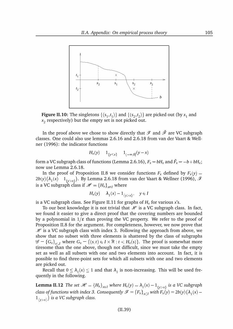
II.A. Appendix: On empirical process theory 105
x2 s1 s2 x1
b
t1
t2
Figure II.10: The singletons f(s1; t1)g and f(s2; t2)g are picked out (by x1 andx2 respectively) but the empty set is not picked out.
In the proof above we chose to show directly that F and F are VC subgraphclasses. One could also use lemmas 2.6.16 and 2.6.18 from van der Vaart & Well-ner (1996): the indicator functions
Hx(y) = 1fyxg = 1(∞;0(y x)form a VC subgraph class of functions (Lemma 2.6.16), Fx = bHx and Fx =b+bHx;now use Lemma 2.6.18.
In the proof of Proposition II.8 we consider functions Fx defined by Fx(y) =2b(y)λ1(x)1fy>xg. By Lemma 2.6.18 from van der Vaart & Wellner (1996), Fis a VC subgraph class if H = fHxgx2I where
Hx(y) = λ1(x)1fy>xg; y 2 I
is a VC subgraph class. See Figure II.11 for graphs of Hx for various x’s.To our best knowledge it is not trivial that H is a VC subgraph class. In fact,
we found it easier to give a direct proof that the covering numbers are boundedby a polynomial in 1=ε than proving the VC property. We refer to the proof ofProposition II.8 for the argument. For completeness, however, we now prove thatH is a VC subgraph class with index 3. Following the approach from above, weshow that no subset with three elements is shattered by the class of subgraphsG = fGxgx2I where Gx = f(s; t) 2 IR : t < Hx(s)g. The proof is somewhat moretiresome than the one above, though not difficult, since we must take the emptyset as well as all subsets with one and two elements into account. In fact, it ispossible to find three-point sets for which all subsets with one and two elementsare picked out.
Recall that 0 λ1(x) 1 and that λ1 is non-increasing. This will be used fre-quently in the following.
Lemma II.12 The set H = fHxgx2I where Hx(y) = λ1(x)1fy>xg is a VC subgraph
class of functions with index 3. ConsequentlyF = fFxgx2I with Fx(y) = 2b(y)λ1(x)1fy>xg is a VC subgraph class.
(II.39)
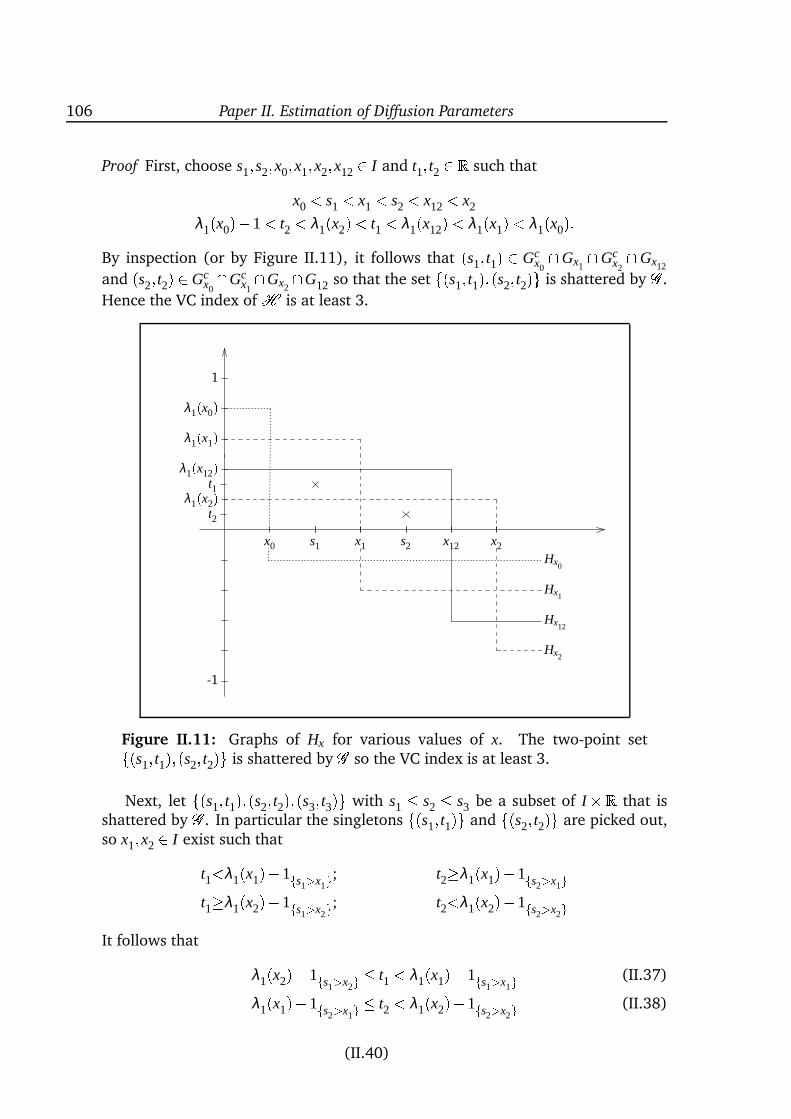
106 Paper II. Estimation of Diffusion Parameters
Proof First, choose s1;s2;x0;x1;x2;x122 I and t1; t2 2 R such that
x0 < s1 < x1 < s2 < x12 < x2
λ1(x0)1< t2 < λ1(x2)< t1 < λ1(x12)< λ1(x1)< λ1(x0):By inspection (or by Figure II.11), it follows that (s1; t1) 2 Gc
x0\Gx1
\Gcx2\Gx12
and (s2; t2) 2 Gcx0\Gc
x1\Gx2
\G12 so that the set f(s1; t1);(s2; t2)g is shattered by G .
Hence the VC index of H is at least 3.
x1 x2
Hx0
Hx1
Hx12
Hx2
λ1(x2)λ1(x1)λ1(x0)1
-1
λ1(x12)x0 s1 s2 x12
t1
t2
Figure II.11: Graphs of Hx for various values of x. The two-point setf(s1; t1);(s2; t2)g is shattered by G so the VC index is at least 3.
Next, let f(s1; t1);(s2; t2);(s3; t3)g with s1 s2 s3 be a subset of IR that isshattered by G . In particular the singletons f(s1; t1)g and f(s2; t2)g are picked out,so x1;x2 2 I exist such that
t1<λ1(x1)1fs1>x1g; t2λ1(x1)1fs2>x1gt1λ1(x2)1fs1>x2g; t2<λ1(x2)1fs2>x2g
It follows that
λ1(x2)1fs1>x2g t1 < λ1(x1)1fs1>x1g (II.37)
λ1(x1)1fs2>x1g t2 < λ1(x2)1fs2>x2g (II.38)
(II.40)
II.A. Appendix: On empirical process theory 107
Hence, if s2 x1 then λ1(x1) < λ1(x2) 1fs2>x2g implying s2 x2 since λ1 is non-
negative. Then (II.37) and (II.38) yields λ1(x2) < λ1(x1) and λ1(x1) < λ1(x2) re-spectively. Similarly if s1 > x1 so we conclude that s1 x1 < s2.
By symmetry we obtain
s1 x1 < s2 x2 < s3
if all three singletons f(s1; t1)g, f(s2; t2)g and f(s3; t3)g are picked out. Hence,
t1<λ1(x1); t2λ1(x1)1; t3λ1(x1)1t1λ1(x2); t2<λ1(x2); t3λ1(x2)1
and
t1λ1(x3)1fs1>x3g; t2λ1(x3)1fs2>x3g; t3<λ1(x3)1fs3>x3g:If s1 x3 then λ1(x3) t1 < λ1(x1) and if x3 < s3 then λ1(x1)1 t3 < λ1(x3)1.Hence, we cannot have s1 x3 < s3. There are thus two possibilities; either
x3 s3; t1λ1(x3); t2λ1(x3); t3<λ1(x3) (II.39)
or
x3 < s1; t1λ1(x3)1; t2λ1(x3)1; t3<λ1(x3)1: (II.40)
First, assume that (II.39) holds. Then
s1 x1 < s2 x2 < s3 x3
λ1(x1)1 t3 < λ1(x3) t2 < λ1(x2) t1 < λ1(x1):Also assume that any subsets of f(s1; t1);(s2; t2);(s3; t3)gwith two elements is pickedout. Hence x12;x13;x232 I exist such that
t1<λ1(x12)1fs1>x12g; t2<λ1(x12)1fs2>x12g; t3λ1(x12)1fs3>x12gand similarly for x13 and x23.
Then necessarily s2 x12 < x2, s1 x13 < x1 and s3 x23 < x3. This followsbecause, with short notation:
x12 < s2) t2 < λ1(x12)1 0;
x12 x2) λ1(x12)> t1 > λ1(x2)) x12 < x2;
x13 < s1) t1 < λ1(x13)1< 0;
x13 x1) λ1(x13)> t1 > λ1(x2)) x13 < x2 < s3) λ1(x13)1> t3 > λ1(x1)1) x13 < x1;
x23 x3) λ1(x23)> t2 > λ1(x3)) x23 < x3;
x23 < s3) λ1(x23)1> t3 > λ1(x1)1) x23 < x1 < s2) t2 < λ1(x23)1< 0
(II.41)
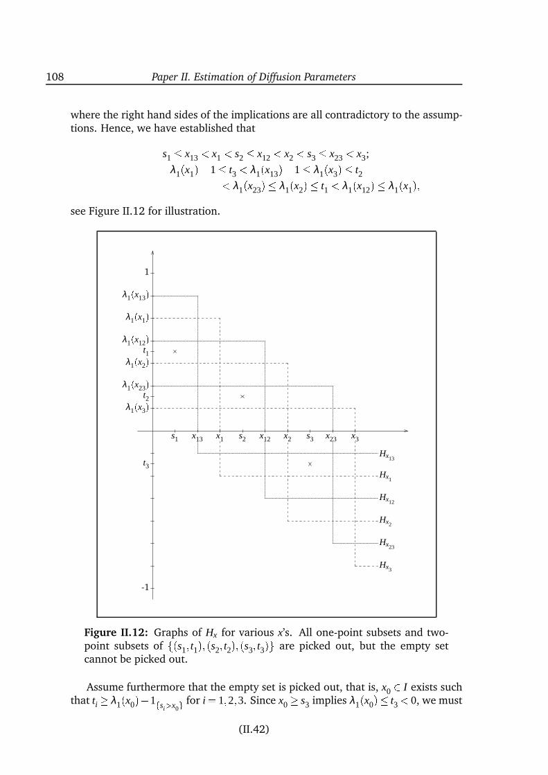
108 Paper II. Estimation of Diffusion Parameters
where the right hand sides of the implications are all contradictory to the assump-tions. Hence, we have established that
s1 x13 < x1 < s2 x12 < x2 < s3 x23 < x3;
λ1(x1)1 t3 < λ1(x13)1 λ1(x3) t2< λ1(x23) λ1(x2) t1 < λ1(x12) λ1(x1);see Figure II.12 for illustration.
λ1(x3)λ1(x23)t2
λ1(x2)λ1(x12)t1
λ1(x1)λ1(x13)1
-1
t3
Hx2
Hx1
Hx13
Hx12
Hx23
Hx3
s1 x13 x1 s2 x12 x2 s3 x23 x3
Figure II.12: Graphs of Hx for various x’s. All one-point subsets and two-point subsets of f(s1; t1);(s2; t2);(s3; t3)g are picked out, but the empty setcannot be picked out.
Assume furthermore that the empty set is picked out, that is, x0 2 I exists suchthat ti λ1(x0)1fsi>x0g for i = 1;2;3. Since x0 s3 implies λ1(x0) t3< 0, we must
(II.42)
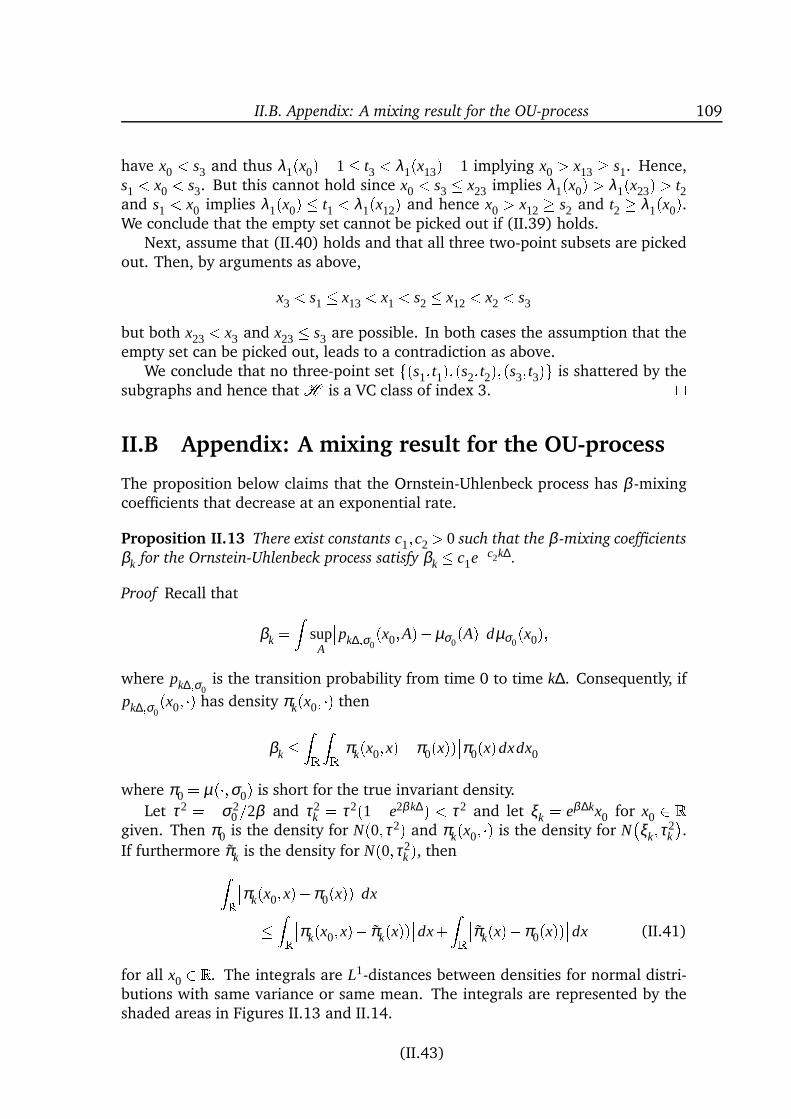
II.B. Appendix: A mixing result for the OU-process 109
have x0 < s3 and thus λ1(x0)1 t3 < λ1(x13)1 implying x0 > x13 s1. Hence,s1 < x0 < s3. But this cannot hold since x0 < s3 x23 implies λ1(x0) > λ1(x23) > t2and s1 < x0 implies λ1(x0) t1 < λ1(x12) and hence x0 > x12 s2 and t2 λ1(x0).We conclude that the empty set cannot be picked out if (II.39) holds.
Next, assume that (II.40) holds and that all three two-point subsets are pickedout. Then, by arguments as above,
x3 < s1 x13 < x1 < s2 x12 < x2 < s3
but both x23 < x3 and x23 s3 are possible. In both cases the assumption that theempty set can be picked out, leads to a contradiction as above.
We conclude that no three-point set f(s1; t1);(s2; t2);(s3; t3)g is shattered by thesubgraphs and hence that H is a VC class of index 3. II.B Appendix: A mixing result for the OU-process
The proposition below claims that the Ornstein-Uhlenbeck process has β -mixingcoefficients that decrease at an exponential rate.
Proposition II.13 There exist constants c1;c2 > 0 such that the β -mixing coefficients
βk for the Ornstein-Uhlenbeck process satisfy βk c1ec2k∆.
Proof Recall that
βk = Zsup
A
pk∆;σ0(x0;A)µσ0
(A)dµσ0(x0);
where pk∆;σ0is the transition probability from time 0 to time k∆. Consequently, if
pk∆;σ0(x0; ) has density πk(x0; ) then
βk ZR ZRπk(x0;x)π0(x))π0(x)dxdx0
where π0 = µ(;σ0) is short for the true invariant density.
Let τ2 = σ20=2β and τ2
k = τ2(1 e2βk∆) < τ2 and let ξk = eβ∆kx0 for x0 2 Rgiven. Then π0 is the density for N(0;τ2) and πk(x0; ) is the density for N
ξk;τ2
k
.
If furthermore πk is the density for N(0;τ2k ), thenZRπk(x0;x)π0(x))dx ZRπk(x0;x) πk(x))dx+ZRπk(x)π0(x))dx (II.41)
for all x0 2 R. The integrals are L1-distances between densities for normal distri-butions with same variance or same mean. The integrals are represented by theshaded areas in Figures II.13 and II.14.
(II.43)
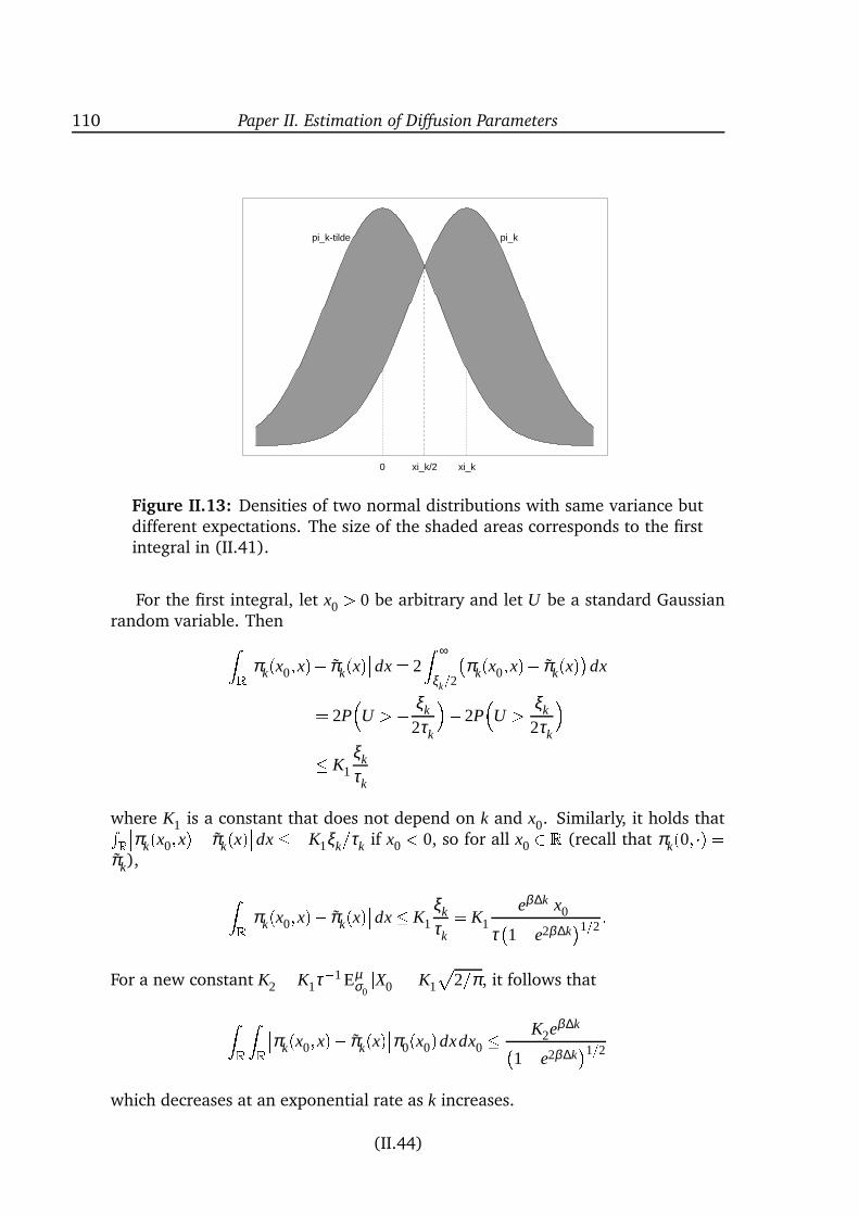
110 Paper II. Estimation of Diffusion Parameters
0 xi_kxi_k/2
pi_k-tilde pi_k
Figure II.13: Densities of two normal distributions with same variance butdifferent expectations. The size of the shaded areas corresponds to the firstintegral in (II.41).
For the first integral, let x0 > 0 be arbitrary and let U be a standard Gaussianrandom variable. ThenZRπk(x0;x) πk(x)dx = 2
Z ∞
ξk=2
πk(x0;x) πk(x)dx= 2P
U > ξk
2τk
2P
U > ξk
2τk
K1ξk
τk
where K1 is a constant that does not depend on k and x0. Similarly, it holds thatRRπk(x0;x) πk(x)dx K1ξk=τk if x0 < 0, so for all x0 2 R (recall that πk(0; ) =πk), ZRπk(x0;x) πk(x)dx K1
ξk
τk= K1
eβ∆kjx0jτ1 e2β∆k
1=2:
For a new constant K2 = K1τ1Eµσ0jX0j= K1
p2=π, it follows thatZR ZRπk(x0;x) πk(x)π0(x0)dxdx0 K2eβ∆k
1 e2β∆k1=2
which decreases at an exponential rate as k increases.
(II.44)
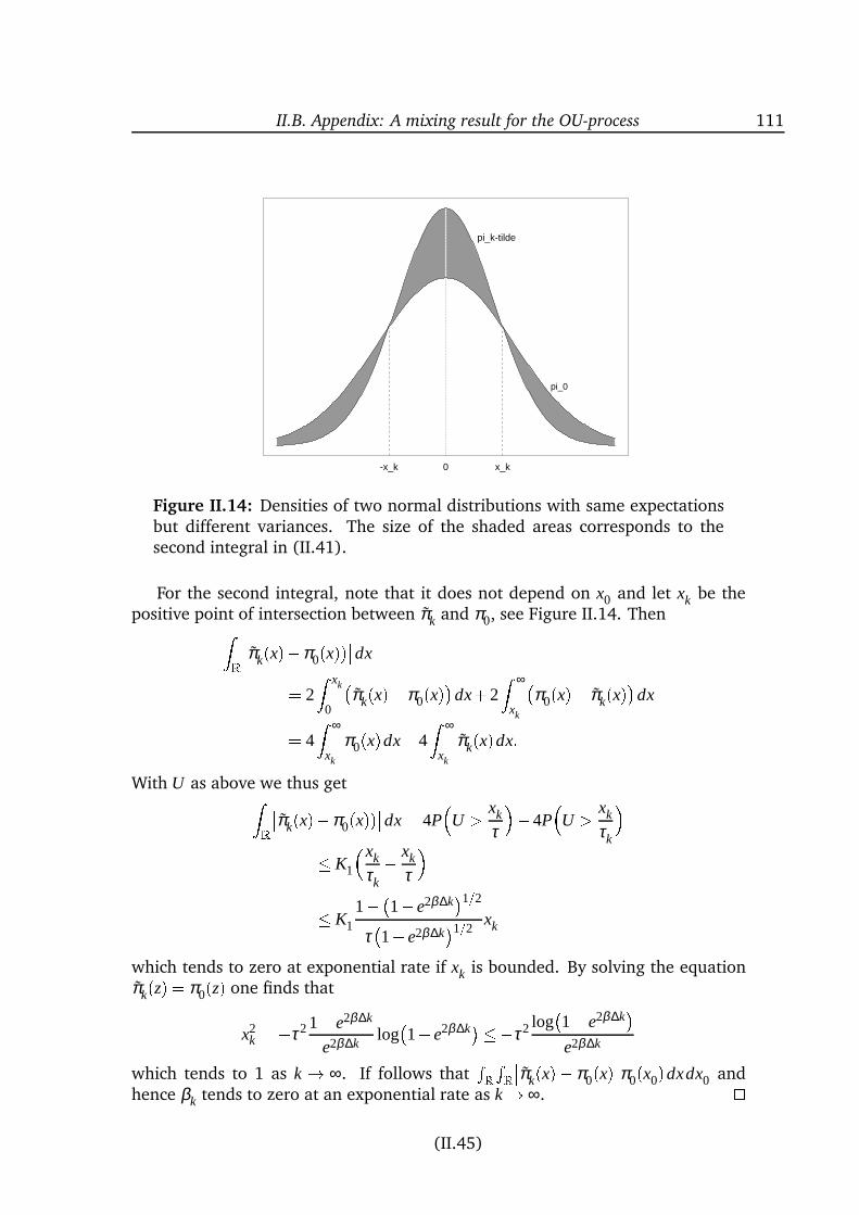
II.B. Appendix: A mixing result for the OU-process 111
0 x_k-x_k
pi_k-tilde
pi_0
Figure II.14: Densities of two normal distributions with same expectationsbut different variances. The size of the shaded areas corresponds to thesecond integral in (II.41).
For the second integral, note that it does not depend on x0 and let xk be thepositive point of intersection between πk and π0, see Figure II.14. ThenZRπk(x)π0(x))dx= 2
Z xk
0
πk(x)π0(x)dx+2
Z ∞
xk
π0(x) πk(x)dx= 4
Z ∞
xk
π0(x)dx4Z ∞
xk
πk(x)dx:With U as above we thus getZRπk(x)π0(x))dx = 4P
U > xk
τ
4P
U > xk
τk
K1
xk
τk xk
τ
K1
1 1 e2β∆k1=2
τ1 e2β∆k
1=2xk
which tends to zero at exponential rate if xk is bounded. By solving the equationπk(z) = π0(z) one finds that
x2k =τ21 e2β∆k
e2β∆klog1 e2β∆kτ2 log
1 e2β∆k
e2β∆k
which tends to 1 as k ! ∞. If follows thatRR RRπk(x) π0(x)π0(x0)dxdx0 and
hence βk tends to zero at an exponential rate as k! ∞. (II.45)

112 Paper II. Estimation of Diffusion Parameters
Acknowledgements Thanks to Søren Feodor Nielsen who provided ideas for theasymptotic results, and to my advisor Martin Jacobsen.
(II.46)
IIISimulated Likelihood
Approximations
for Stochastic Volatility Models
Abstract
The objective of this paper is approximate maximum likelihood estimation forstochastic volatility models. We consider a two-dimensional diffusion process(X ;V) where V is ergodic while X has drift and diffusion coefficient completelydetermined by V . The distribution of V — and thereby also the distribution of X— depends on an unknown parameter θ , and our concern is estimation of θ fromdiscrete-time observations of X . The volatility process V remains unobserved. Weconsider approximate maximum likelihood estimation. For the k’th order approxi-mation we pretend that the observations form a k’th order Markov chain, find thecorresponding approximate log-likelihood function, and maximize it with respectto θ . There is no explicit expression for the approximate log-likelihood function,but it can be calculated by simulation. For each k the method yields consistentand asymptotically normal estimators. Simulations of the model where V is aCox-Ingersoll-Ross model are used for illustration.
Key words
Approximate maximum likelihood estimation; asymptotic normality; consistency;Cox-Ingersoll-Ross process; discretely observed diffusion processes; stochastic vol-atility models.
Publication details
A shorter version of this paper (without Appendix III.A.2, with fewer details onthe Cox-Ingersoll-Ross model and the simulation study and with fewer proofs in-cluded) will be submitted for publication shortly.
114 Paper III. Simulated Likelihood Approximations
III.1 Introduction
We are concerned with inference for continuous-time stochastic volatility models.By stochastic volatility models we will mean models for a pair of processes (X ;V )where V is a latent, positive diffusion process and the observable process X solvesa stochastic differential equation with diffusion term
pV and drift determined by
V as well. The process V is called the volatility process. We consider parametricspecifications of the drift and the diffusion function for V , and the objective isapproximate maximum likelihood estimation based on discrete-time observationsof X .
For a start, consider the classical Black-Scholes model (or geometric Brownianmotion)
dPt = αPt dt + τPt dWt (III.1)
which is (or rather was) often used to model stock prices. The classical option pric-ing formula was derived for this model (Black & Scholes 1973). If P solves (III.1)then logP has constant volatility (squared diffusion) and independent, normallydistributed increments. It is well-known that these properties are inconsistent withempirical findings: studies have revealed that stock returns (and other financialdata) often are dependent, have strongly leptokurtic marginal distributions andexhibit signs of randomly varying variance over time.
In the discrete-time setting ARCH-type models and discrete-time stochasticvolatility models have been used for modeling such phenomena. See Shephard(1996) for an overview of both model types. However, for derivative pricing (andrelated problems) it may be advantageous to use continuous-time models, retain-ing the Black-Scholes machinery at our disposal. Also, irregularly sampled dataare easier to handle for continuous-time models than for discrete-time models.
Of course one could generate the above features by simply allowing for non-linear drift and diffusion functions for the price process. In the stochastic volatilityframework, however, the linear structure of the equation for P is retained, but anadditional source of variability is introduced: the constant τ in (III.1) is replacedby the value of a latent diffusion process
pV . The modified equation for P is thus
dPt = αPt dt +pVtPt dWt : (III.2)
In this paper we shall consider models given by
dXt = ξ (Vt)dt +pVt dWt
dVt = b(Vt ;θ)dt +σ(Vt;θ)dWt
where V is stationary and ergodic. With P = eX it follows by Itô’s formula that thismodel is equivalent to (III.2) if ξ (v) = αv=2 (and α is known). Hence, a possibleapplication of the model is for the logarithm of a stock price.
The drift and diffusion for V are parameter dependent, and we shall be inter-ested in estimation of θ from equidistant observations X0;X∆; : : : ;Xn∆ of X . The
(III.2)
III.1. Introduction 115
volatility process V remains unobserved. Conditional on V the above model isvery simple as increments of X are independent and Gaussian: Zi = Xi∆X(i1)∆ N(Mi;Si) where Mi = R i∆(i1)∆ ξ (Vs)ds and Si = R i∆(i1)∆Vs ds:
For the above model to make sense, we must model V as a positive pro-cess. Various models were suggested in the late eighties and early nineties: Vwas modeled as a geometric Brownian motion (Hull & White 1987), as a Cox-Ingersoll-Ross process (Hull & White 1988, Heston 1993), as the exponential ofa Ornstein-Uhlenbeck process (Wiggins 1987, Chesney & Scott 1989) and as asquared Ornstein-Uhlenbeck process (Scott 1987, Stein & Stein 1991).
The above papers all focus on pricing of a European call option written on astock with price process P. Pricing is investigated for fixed value of the parameterθ in the equation for V , and the majority of the papers pay no or little attentionto estimation of θ . Only Scott (1987) and Chesney & Scott (1989) address theproblem seriously and derive moment-like estimators for the parameters. Morerecently, several estimation approaches have been suggested, some of which haveearlier been applied for the discrete-time versions of the models; see Shephard(1996) and Ghysels et al. (1996) for surveys.
Genon-Catalot et al. (1999) consider the approximation that the incrementsZ1; : : : ;Zn are independent and identically distributed with conditional distributionof Z1 given V equal to N(∆ξ (V0);∆V0). The estimators are consistent as n!∞ onlyif the time-step ∆ decreases to zero as n increases. For (large) fixed values of ∆ thebias may be considerable. Also, only estimation of parameters from the station-ary distribution of V is possible. In another paper, Genon-Catalot et al. (1998b)consider mean-reverting models for V . Then calculation of various moments ofthe joint distribution of the increments is possible, and estimation is carried outby matching theoretical and empirical moments. For any fixed ∆ the estimatorsso obtained are consistent and asymptotically normal as n increases. However,the simulation study in Section III.7 indicates that there may be serious existenceproblems in practice. The two above methods require no hard numerical com-putations or simulations and are thus quick in practice. As opposed to this mostother methods (and the one suggested in this paper) are quite computationallyintensive.
Nielsen et al. (2000) use a filtering approach where values of V are estimatedtogether with the parameter. This requires that n (that is, the number of obser-vations) differential equations are solved by numerical methods. Eraker (1998)use a Bayesian approach which requires Markov Chain Monte Carlo simulation ofvalues of V and X at time-points in between those where X is observed as wellas of values of θ ; see also Elerian et al. (2000). The so-called efficient method ofmoments (Gallant & Tauchen 1996) is applied to a stochastic volatility model byAndersen & Lund (1997). Finally, Sørensen (1999) studies prediction-based esti-mating functions. Particular attention is paid to the case where for a function fand an integer k, each term in the estimating function is given in terms of the valuef (Zi) and its projection on some space determined by the previous k incrementsZik+1; : : : ;Zi. Typically, the projections must be calculated by simulation.
(III.3)
116 Paper III. Simulated Likelihood Approximations
The method suggested in this paper is somewhat related since we also choosea number k 0 and base inference on k lags of the increments. For a given value ofk the idea is to pretend that (Z1;Z2; : : :) is k’th order Markov, find the correspondingapproximate likelihood function, and maximize it with respect to θ . In particulark = 0 corresponds to pretending that observations are independent, drawn fromthe stationary distribution (and may thus be interpreted as an improvement of themethod by Genon-Catalot et al. (1999) who use an approximation to the stationarydensity), and k = 1 corresponds to pretending that observations are Markov.
There is no explicit expression for the k-lag conditional density, but we can ex-press it in terms of expectations with respect to the distribution of (Vt)0t(k+1)∆and therefore calculate it by simulation of V on the interval from zero to (k+1)∆.For any fixed ∆ and any k 0 the approximate score function in unbiased and (un-der regularity conditions, of course) the estimator is consistent and asymptoticallynormal as the number of observations increases.
We use the model where ξ 0 and V is a Cox-Ingersoll-Ross process as exampleand use the method on simulated data. If the parameter in the diffusion functionis considered known we obtain satisfactory estimates even for k = 0, whereas wefor all three parameters unknown must use a larger k, say 4, to get reasonableestimates.
The paper is organized as follows. In Section III.2 we discuss the model andits probabilistic properties. We introduce the likelihood approximations and theestimation method in Section III.3 and discuss the computational aspects in Sec-tion III.4. The efficiency of the estimators is briefly discussed in Section III.6. InSection III.7 we discuss the Cox-Ingersoll-Ross model for V in detail, try out the es-timation method on simulated data and compare with simple moment estimators.We conclude in Section III.8.
III.2 Model and basic assumptions
In this section we discuss the model and the basic assumptions in detail. Let(W;W ) = f(Wt;Wt)gt0 be a standard two-dimensional Brownian motion definedon a filtered probability space (Ω;F ;Ft;Pr) satisfying the usual conditions andlet UX ;UV : Ω ! R be F0-measurable random variables, mutually independentand independent of (W;W). Furthermore, let (X ;V) = f(Xt;Vt)gt0 be a two-dimen-sional diffusion process governed by the stochastic differential equations
dXt = ξ (Vt)dt +pVt dWt ; X0 =UX (III.3)
dVt = b(Vt ;θ)dt +σ(Vt;θ)dWt ; V0 =UV : (III.4)
Here θ is an unknown p-dimensional parameter from the parameter space Θ Rp
and V is positive Pr-almost surely. The functions ξ : (0;∞)! R, b : (0;∞)Θ! Rand σ : (0;∞)Θ ! (0;∞) are known and continuous (for b and σ : with respectto the state variable).
(III.4)
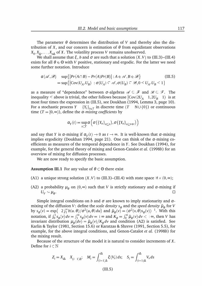
III.2. Model and basic assumptions 117
The parameter θ determines the distribution of V and thereby also the dis-tribution of X , and our concern is estimation of θ from equidistant observationsX0;X∆; : : : ;Xn∆ of X . The volatility process V remains unobserved.
We shall assume that ξ , b and σ are such that a solution (X ;V) to (III.3)–(III.4)exists for all θ 2 Θ with V positive, stationary and ergodic. For the latter we needsome further notation. Introduce
α(A ;B) = supPr(A\B)Pr(A)Pr(B) : A 2A ;B 2B (III.5)= supCov(UA;UB) : σ(UA)A ;σ(UB)B;0UA;UB 1
as a measure of “dependence” between σ -algebras A F and B F . Theinequality above is trivial, the other follows because
Cov(2UA1;2UB1) is atmost four times the expression in (III.5), see Doukhan (1994, Lemma 3, page 10).For a stochastic process Y = fYtgt2T in discrete time (T = N [f0g) or continuoustime (T = [0;∞)), define the α-mixing coefficients by
αY (t) = sups2T
α
σfYugus
;σfYugus+t
and say that Y is α-mixing if αY (t)! 0 as t ! ∞. It is well-known that α-mixingimplies ergodicity (Doukhan 1994, page 21). One can think of the α-mixing co-efficients as measures of the temporal dependence in Y . See Doukhan (1994), forexample, for the general theory of mixing and Genon-Catalot et al. (1998b) for anoverview of mixing for diffusion processes.
We are now ready to specify the basic assumption.
Assumption III.1 For any value of θ 2 Θ there exist
(A1) a unique strong solution (X ;V) to (III.3)–(III.4) with state space R (0;∞);(A2) a probability µθ on (0;∞) such that V is strictly stationary and α-mixing if
UV µθ . Simple integral conditions on b and σ are known to imply stationarity and α-
mixing of the diffusion V : define the scale density sθ and the speed density µθ for Vby sθ (v) = exp
2R v
1 b(u;θ)=σ2(u;θ)du
and µθ (v) = (σ2(v;θ)sθ (v))1. With this
notation, ifR 1
0 sθ (v)dv = R ∞1 sθ (v)dv = +∞ and Kθ = R ∞
0 µθ (v)dv < +∞, then V hasinvariant distribution µθ (dv) = µθ (v)=Kθ dv and condition (A2) is satisfied. SeeKarlin & Taylor (1981, Section 15.6) or Karatzas & Shreve (1991, Section 5.5), forexample, for the above integral conditions, and Genon-Catalot et al. (1998b) forthe mixing result.
Because of the structure of the model it is natural to consider increments of X .Define for i 2 N
Zi = Xi∆X(i1)∆; Mi = Z i∆(i1)∆ ξ (Vs)ds; Si = Z i∆(i1)∆Vs ds
(III.5)
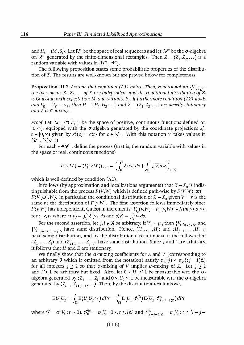
118 Paper III. Simulated Likelihood Approximations
and Hi = (Mi;Si). Let R∞ be the space of real sequences and letB∞ be the σ -algebraon R∞ generated by the finite-dimensional rectangles. Then Z = (Z1;Z2; : : :) is arandom variable with values in (R∞ ;B∞).
The following proposition states some probabilistic properties of the distribu-tion of Z. The results are well-known but are proved below for completeness.
Proposition III.2 Assume that condition (A1) holds. Then, conditional on fVtgt0,
the increments Z1;Z2; : : : of X are independent and the conditional distribution of Ziis Gaussian with expectation Mi and variance Si. If furthermore condition (A2) holds
and V0 = UV µθ , then H = (H1;H2; : : :) and Z = (Z1;Z2; : : :) are strictly stationary
and Z is α-mixing.
Proof Let (C+;B(C+)) be the space of positive, continuous functions defined on[0;∞), equipped with the σ -algebra generated by the coordinate projections xÆt ,t 2 [0;∞) given by xÆt (c) = c(t) for c 2 C+. With this notation V takes values in(C+;B(C+)).
For each v 2 C+, define the process (that is, the random variable with values inthe space of real, continuous functions)
F(v;W ) = Ft(v;W)t0 = Z t
0ξ (vs)ds+Z t
0
pvs dws
t0
which is well-defined by condition (A1).It follows (by approximation and localizations arguments) that X X0 is indis-
tinguishable from the process F(V;W) which is defined path-wise by F(V;W)(ω) =F(V (ω);W ). In particular, the conditional distribution of X X0 given V = v is thesame as the distribution of F(v;W). The first assertion follows immediately sinceF(v;W ) has independent, Gaussian increments: Ft2
(v;W)Ft1(v;W ) N(m(v);s(v))
for t1 < t2 where m(v) = R t2t1
ξ (vs)ds and s(v) = R t2t1
vs ds.
For the second assertion, let j; l 2 N be arbitrary. If V0 µθ then fVtg0tl∆ andfVtg j∆t(l+ j)∆ have same distribution. Hence, (H1; : : : ;Hl) and (H j+1; : : : ;H j+l)have same distribution, and by the distributional result above it the follows that(Z1; : : : ;Zl) and (Z j+1; : : : ;Z j+l) have same distribution. Since j and l are arbitrary,
it follows that H and Z are stationary.We finally show that the α-mixing coefficients for Z and V (corresponding to
an arbitrary θ which is omitted from the notation) satisfy αZ( j) αV
( j 1)∆for all integers j 2 so that α-mixing of V implies α-mixing of Z. Let j 2and l 1 be arbitrary but fixed. Also, let 0U1 1 be measurable wrt. the σ -algebra generated by (Z1; : : : ;Zl) and 0U2 1 be measurable wrt. the σ -algebragenerated by (Zl+1;Zl+ j+1; : : :). Then, by the distribution result above,
EU1U2 = ZΩ
EU1U2jG dPr = Z
ΩEU1jG l∆
0
EU2jG ∞(l+ j1)∆dPr
where G = σ(Vt : t 0), G l∆0 = σ(Vt : 0 t l∆) and G ∞(l+ j1)∆ = σ(Vt : t (l + j
(III.6)
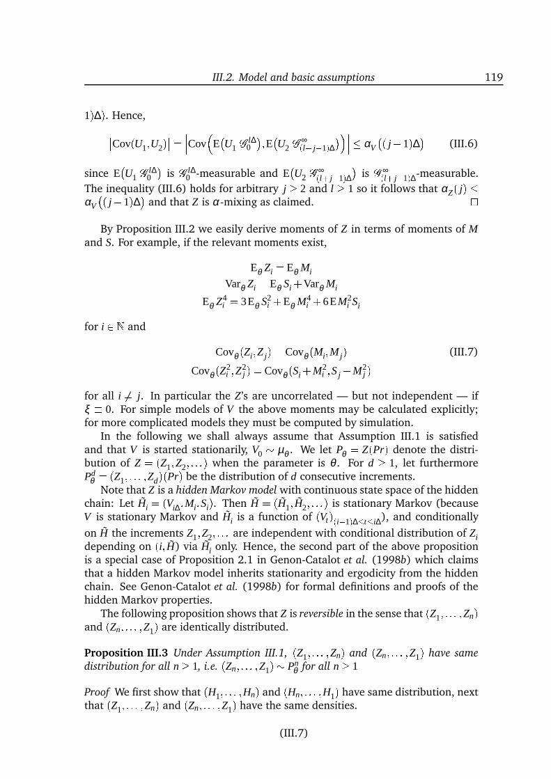
III.2. Model and basic assumptions 119
1)∆). Hence,Cov(U1;U2)= Cov
EU1jG l∆
0
;EU2jG ∞(l+ j1)∆ αV
( j1)∆ (III.6)
since EU1jG l∆
0
is G l∆
0 -measurable and EU2jG ∞(l+ j1)∆ is G ∞(l+ j1)∆-measurable.
The inequality (III.6) holds for arbitrary j 2 and l 1 so it follows that αZ( j)αV
( j1)∆ and that Z is α-mixing as claimed. By Proposition III.2 we easily derive moments of Z in terms of moments of M
and S. For example, if the relevant moments exist,
Eθ Zi = Eθ Mi
Varθ Zi = Eθ Si +Varθ Mi
Eθ Z4i = 3Eθ S2
i +Eθ M4i +6EM2
i Si
for i 2 N and
Covθ (Zi;Z j) = Covθ (Mi;M j) (III.7)
Covθ (Z2i ;Z2
j ) = Covθ (Si +M2i ;S j +M2
j )for all i 6= j. In particular the Z’s are uncorrelated — but not independent — ifξ 0. For simple models of V the above moments may be calculated explicitly;for more complicated models they must be computed by simulation.
In the following we shall always assume that Assumption III.1 is satisfiedand that V is started stationarily, V0 µθ . We let Pθ = Z(Pr) denote the distri-bution of Z = (Z1;Z2; : : :) when the parameter is θ . For d 1, let furthermorePd
θ = (Z1; : : : ;Zd)(Pr) be the distribution of d consecutive increments.Note that Z is a hidden Markov model with continuous state space of the hidden
chain: Let Hi = (Vi∆;Mi;Si). Then H = (H1; H2; : : :) is stationary Markov (becauseV is stationary Markov and Hi is a function of (Vt)(i1)∆ti∆), and conditionally
on H the increments Z1;Z2; : : : are independent with conditional distribution of Zidepending on (i; H) via Hi only. Hence, the second part of the above propositionis a special case of Proposition 2.1 in Genon-Catalot et al. (1998b) which claimsthat a hidden Markov model inherits stationarity and ergodicity from the hiddenchain. See Genon-Catalot et al. (1998b) for formal definitions and proofs of thehidden Markov properties.
The following proposition shows that Z is reversible in the sense that (Z1; : : : ;Zn)and (Zn; : : : ;Z1) are identically distributed.
Proposition III.3 Under Assumption III.1, (Z1; : : : ;Zn) and (Zn; : : : ;Z1) have same
distribution for all n 1, i.e. (Zn; : : : ;Z1) Pnθ for all n 1
Proof We first show that (H1; : : : ;Hn) and (Hn; : : : ;H1) have same distribution, nextthat (Z1; : : : ;Zn) and (Zn; : : : ;Z1) have the same densities.
(III.7)
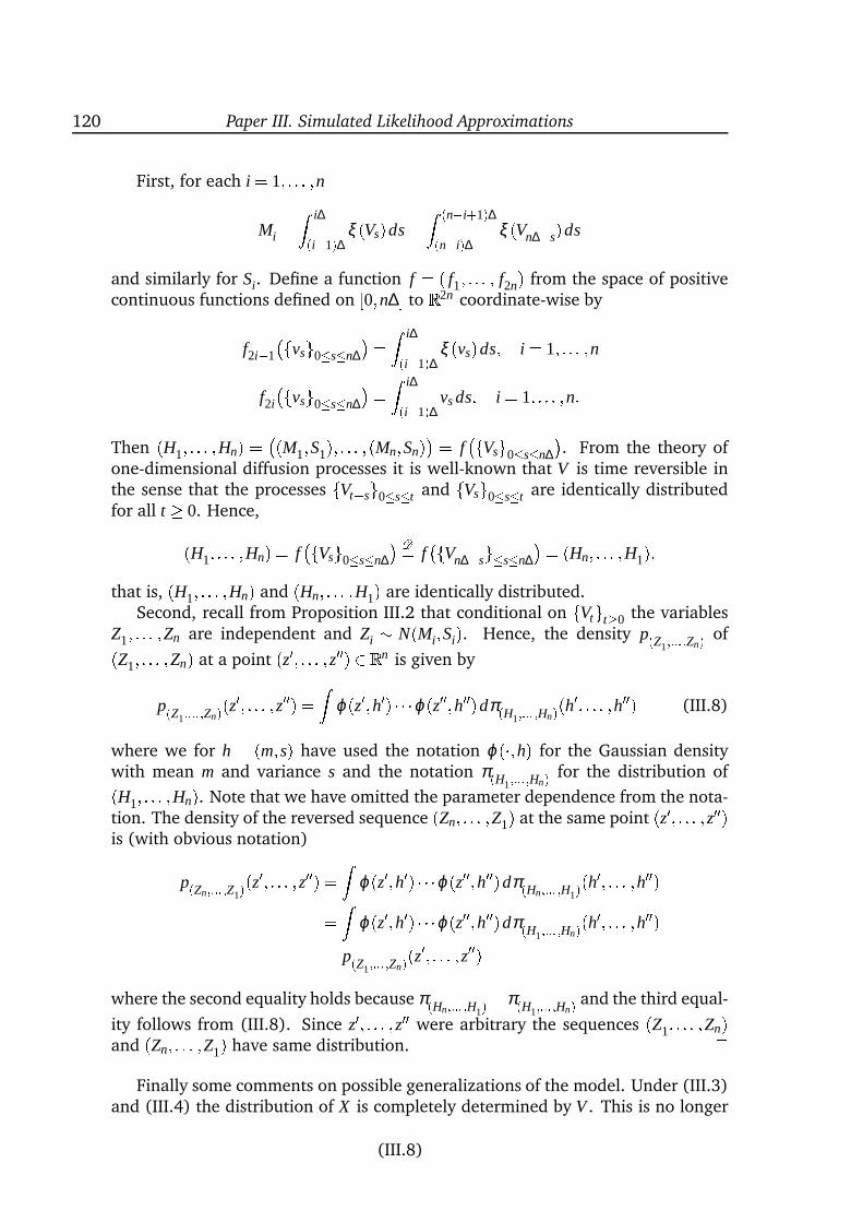
120 Paper III. Simulated Likelihood Approximations
First, for each i = 1; : : : ;nMi = Z i∆(i1)∆ ξ (Vs)ds = Z (ni+1)∆(ni)∆ ξ (Vn∆s)ds
and similarly for Si. Define a function f = ( f1; : : : ; f2n) from the space of positivecontinuous functions defined on [0;n∆ to R2n coordinate-wise by
f2i1
fvsg0sn∆= Z i∆(i1)∆ ξ (vs)ds; i = 1; : : : ;n
f2i
fvsg0sn∆= Z i∆(i1)∆ vs ds; i = 1; : : : ;n:
Then (H1; : : : ;Hn) = (M1;S1); : : : ;(Mn;Sn) = ffVsg0sn∆
. From the theory of
one-dimensional diffusion processes it is well-known that V is time reversible inthe sense that the processes fVtsg0st and fVsg0st are identically distributedfor all t 0. Hence,(H1; : : : ;Hn) = f
fVsg0sn∆ D= f
fVn∆sgsn∆= (Hn; : : : ;H1);
that is, (H1; : : : ;Hn) and (Hn; : : : ;H1) are identically distributed.Second, recall from Proposition III.2 that conditional on fVtgt0 the variables
Z1; : : : ;Zn are independent and Zi N(Mi;Si). Hence, the density p(Z1;::: ;Zn) of(Z1; : : : ;Zn) at a point (z0; : : : ;z00) 2 Rn is given by
p(Z1;::: ;Zn)(z0; : : : ;z00) = Zϕ(z0;h0) ϕ(z00;h00)dπ(H1;::: ;Hn)(h0; : : : ;h00) (III.8)
where we for h = (m;s) have used the notation ϕ(;h) for the Gaussian densitywith mean m and variance s and the notation π(H1;::: ;Hn) for the distribution of(H1; : : : ;Hn). Note that we have omitted the parameter dependence from the nota-tion. The density of the reversed sequence (Zn; : : : ;Z1) at the same point (z0; : : : ;z00)is (with obvious notation)
p(Zn;::: ;Z1)(z0; : : : ;z00) = Zϕ(z0;h0) ϕ(z00;h00)dπ(Hn;::: ;H1)(h0; : : : ;h00)= Zϕ(z0;h0) ϕ(z00;h00)dπ(H1;::: ;Hn)(h0; : : : ;h00)= p(Z1;::: ;Zn)(z0; : : : ;z00)
where the second equality holds because π(Hn;::: ;H1)= π(H1;::: ;Hn) and the third equal-
ity follows from (III.8). Since z0; : : : ;z00 were arbitrary the sequences (Z1; : : : ;Zn)and (Zn; : : : ;Z1) have same distribution.
Finally some comments on possible generalizations of the model. Under (III.3)and (III.4) the distribution of X is completely determined by V . This is no longer
(III.8)
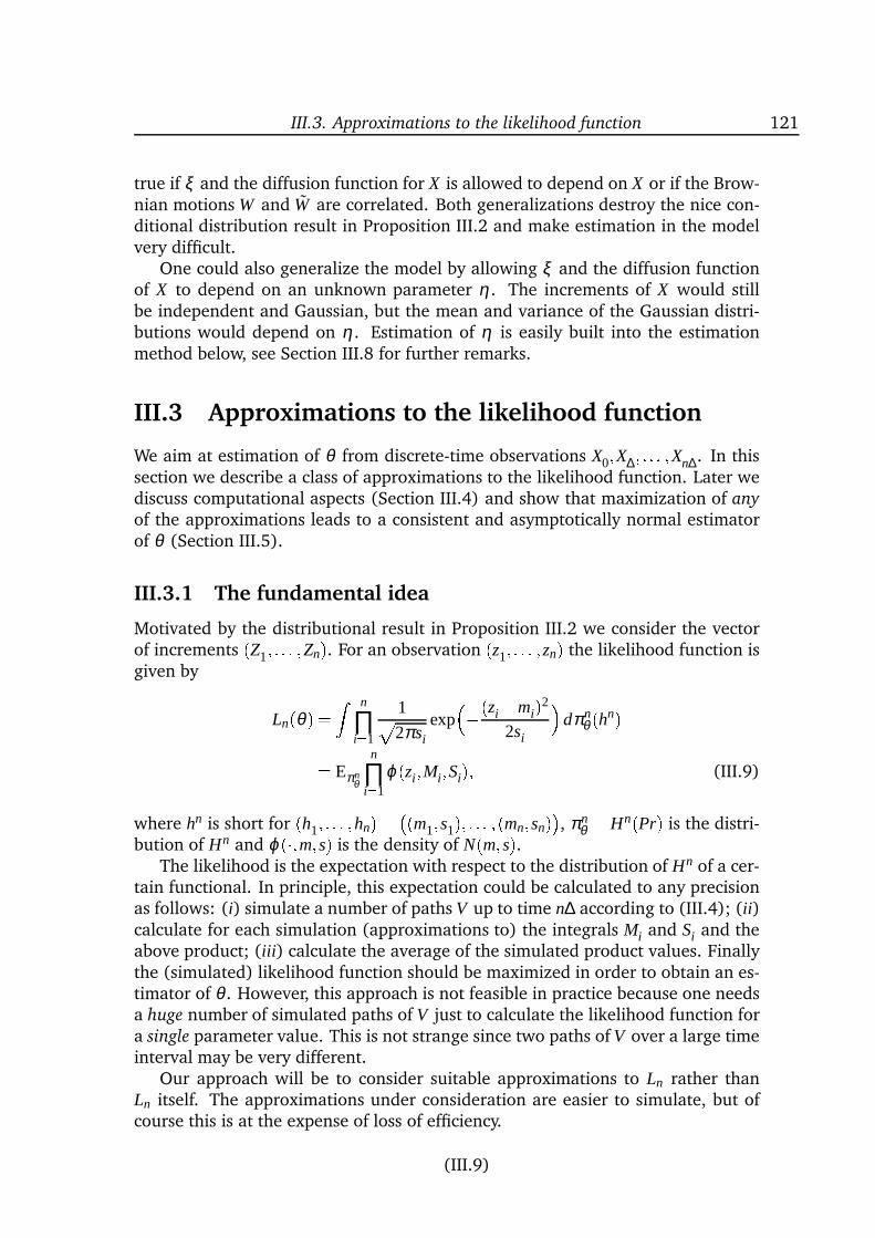
III.3. Approximations to the likelihood function 121
true if ξ and the diffusion function for X is allowed to depend on X or if the Brow-nian motions W and W are correlated. Both generalizations destroy the nice con-ditional distribution result in Proposition III.2 and make estimation in the modelvery difficult.
One could also generalize the model by allowing ξ and the diffusion functionof X to depend on an unknown parameter η. The increments of X would stillbe independent and Gaussian, but the mean and variance of the Gaussian distri-butions would depend on η. Estimation of η is easily built into the estimationmethod below, see Section III.8 for further remarks.
III.3 Approximations to the likelihood function
We aim at estimation of θ from discrete-time observations X0;X∆; : : : ;Xn∆. In thissection we describe a class of approximations to the likelihood function. Later wediscuss computational aspects (Section III.4) and show that maximization of any
of the approximations leads to a consistent and asymptotically normal estimatorof θ (Section III.5).
III.3.1 The fundamental idea
Motivated by the distributional result in Proposition III.2 we consider the vectorof increments (Z1; : : : ;Zn). For an observation (z1; : : : ;zn) the likelihood function isgiven by
Ln(θ) = Z n
∏i=1
1p2πsi
exp(zimi)2
2si
dπn
θ (hn)= Eπnθ
n
∏i=1
ϕ(zi;Mi;Si); (III.9)
where hn is short for (h1; : : : ;hn) = (m1;s1); : : : ;(mn;sn), πnθ = Hn(Pr) is the distri-
bution of Hn and ϕ(;m;s) is the density of N(m;s).The likelihood is the expectation with respect to the distribution of Hn of a cer-
tain functional. In principle, this expectation could be calculated to any precisionas follows: (i) simulate a number of paths V up to time n∆ according to (III.4); (ii)calculate for each simulation (approximations to) the integrals Mi and Si and theabove product; (iii) calculate the average of the simulated product values. Finallythe (simulated) likelihood function should be maximized in order to obtain an es-timator of θ . However, this approach is not feasible in practice because one needsa huge number of simulated paths of V just to calculate the likelihood function fora single parameter value. This is not strange since two paths of V over a large timeinterval may be very different.
Our approach will be to consider suitable approximations to Ln rather thanLn itself. The approximations under consideration are easier to simulate, but ofcourse this is at the expense of loss of efficiency.
(III.9)
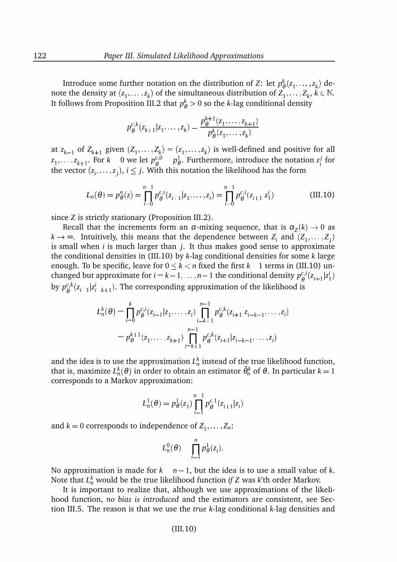
122 Paper III. Simulated Likelihood Approximations
Introduce some further notation on the distribution of Z: let pkθ (z1; : : : ;zk) de-
note the density at (z1; : : : ;zk) of the simultaneous distribution of Z1; : : : ;Zk, k 2 N.
It follows from Proposition III.2 that pkθ > 0 so the k-lag conditional density
pc;kθ (zk+1jz1; : : : ;zk) = pk+1
θ (z1; : : : ;zk+1)pk
θ (z1; : : : ;zk)at zk+1 of Zk+1 given (Z1; : : : ;Zk) = (z1; : : : ;zk) is well-defined and positive for all
z1; : : : ;zk+1. For k = 0 we let pc;0θ = p1
θ . Furthermore, introduce the notation z ji
for
the vector (zi; : : : ;z j), i j. With this notation the likelihood has the form
Ln(θ) = pnθ (z) = n1
∏i=0
pc;iθ (zi+1jz1; : : : ;zi) = n1
∏i=0
pc;iθ (zi+1jzi
1) (III.10)
since Z is strictly stationary (Proposition III.2).Recall that the increments form an α-mixing sequence, that is αZ(k)! 0 as
k ! ∞. Intuitively, this means that the dependence between Zi and (Z1; : : : ;Z j)is small when i is much larger than j. It thus makes good sense to approximatethe conditional densities in (III.10) by k-lag conditional densities for some k largeenough. To be specific, leave for 0 k < n fixed the first k+1 terms in (III.10) un-changed but approximate for i = k+1; : : : ;n1 the conditional density pc;i
θ (zi+1jzi1)
by pc;kθ (zi+1jzi
ik+1). The corresponding approximation of the likelihood is
Lkn(θ) = k
∏i=0
pc;iθ (zi+1jz1; : : : ;zi) n1
∏i=k+1
pc;kθ (zi+1jzik+1; : : : ;zi)= pk+1
θ (z1; : : : ;zk+1) n1
∏i=k+1
pc;kθ (zi+1jzik+1; : : : ;zi)
and the idea is to use the approximation Lkn instead of the true likelihood function,
that is, maximize Lkn(θ) in order to obtain an estimator θ k
n of θ . In particular k = 1corresponds to a Markov approximation:
L1n(θ) = p1
θ (z1)n1
∏i=1
pc;1θ (zi+1jzi)
and k = 0 corresponds to independence of Z1; : : : ;Zn:
L0n(θ) = n
∏i=1
p1θ (zi):
No approximation is made for k = n1, but the idea is to use a small value of k.Note that Lk
n would be the true likelihood function if Z was k’th order Markov.It is important to realize that, although we use approximations of the likeli-
hood function, no bias is introduced and the estimators are consistent, see Sec-tion III.5. The reason is that we use the true k-lag conditional k-lag densities and
(III.10)
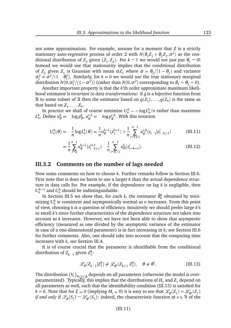
III.3. Approximations to the likelihood function 123
not some approximation. For example, assume for a moment that Z is a strictlystationary auto-regressive process of order 2 with N(θ1Z1+ θ2Z2;σ2) as the con-ditional distribution of Z3 given (Z1;Z2). For k = 1 we would not just put θ1 = 0!Instead we would use that stationarity implies that the conditional distributionof Z2 given Z1 is Gaussian with mean αZ1 where α = θ2=(1 θ1) and varianceσ2
1 = σ2=(1 θ21). Similarly, for k = 0 we would use the true stationary marginal
distribution N(0;σ21=(1α2)) (rather than N(0;σ2) corresponding to θ1 = θ2 = 0).
Another important property is that the k’th order approximate maximum likeli-hood estimator is invariant to data transformations: if g is a bijective function fromR to some subset of R then the estimator based on g(Z1); : : : ;g(Zn) is the same asthat based on Z1; : : : ;Zn.
In practice we shall of course minimize U kn = logLk
n=n rather than maximizeLk
n. Define ukθ = logpk
θ , uc;kθ = logpc;k
θ . With this notation
U kn (θ) =1
nlogLk
n(θ) = 1n
uk+1θ (zk+1
1 )+ 1n
n1
∑i=k+1
uc;kθ (zi+1jzi
ik+1) (III.11)= 1n
n1
∑i=k
uk+1θ (zi+1
ik+1) 1n
n1
∑i=k+1
ukθ (zi
ik+1): (III.12)
III.3.2 Comments on the number of lags needed
Now some comments on how to choose k. Further remarks follow in Section III.6.First note that is does no harm to use a larger k than the actual dependence struc-ture in data calls for. For example, if the dependence on lag k is negligible, thenU k1
n and U kn should be indistinguishable.
In Section III.5 we show that, for each k, the estimator θ kn obtained by mini-
mizing U kn is consistent and asymptotically normal as n increases. From this point
of view, choosing k is a question of efficiency. Intuitively we should prefer large k’sto small k’s since further characteristics of the dependence structure are taken intoaccount as k increases. However, we have not been able to show that asymptoticefficiency (measured as one divided by the asymptotic variance of the estimatorin case of a one-dimensional parameter) is in fact increasing in k; see Section III.6for further comments. Also, one should take into account that the computing timeincreases with k, see Section III.4.
It is of course crucial that the parameter is identifiable from the conditionaldistribution of Zk+1 given Zk
1:Lθ (Zk+1jZk1) 6=Lθ 0(Zk+1jZk
1); θ 6= θ 0: (III.13)
The distribution fVtg0t∆ depends on all parameters (otherwise the model is over-parametrized). Typically, this implies that the distributions of H1 and Z1 depend onall parameters as well, such that the identifiability condition (III.13) is satisfied fork = 0. Note that for ξ 0 (implying Mi 0) it is easy to see thatLθ (Z1) =Lθ 0(Z1)if and only if Lθ (S1) =Lθ 0(S1): indeed, the characteristic function at x 2 R of the
(III.11)
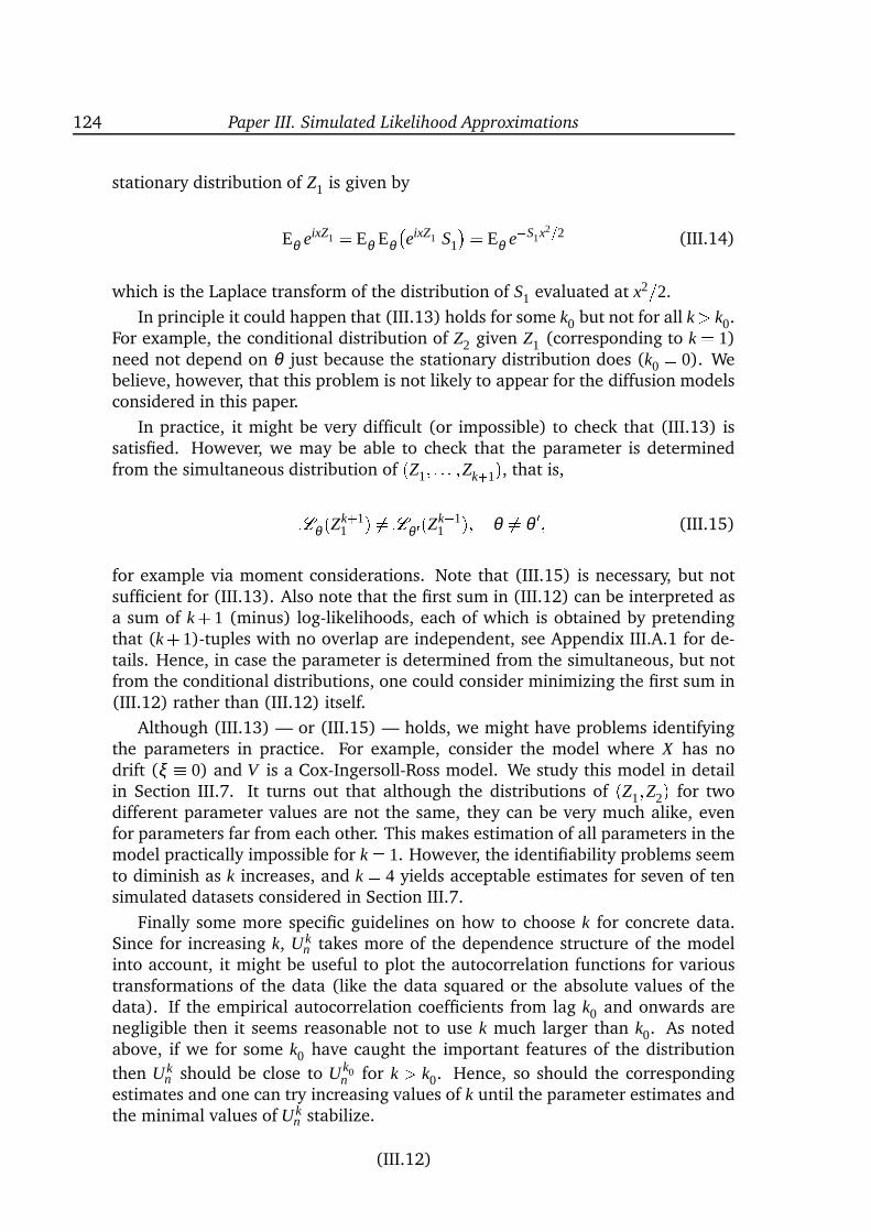
124 Paper III. Simulated Likelihood Approximations
stationary distribution of Z1 is given by
Eθ eixZ1 = Eθ EθeixZ1jS1
= Eθ eS1x2=2 (III.14)
which is the Laplace transform of the distribution of S1 evaluated at x2=2.
In principle it could happen that (III.13) holds for some k0 but not for all k > k0.For example, the conditional distribution of Z2 given Z1 (corresponding to k = 1)need not depend on θ just because the stationary distribution does (k0 = 0). Webelieve, however, that this problem is not likely to appear for the diffusion modelsconsidered in this paper.
In practice, it might be very difficult (or impossible) to check that (III.13) issatisfied. However, we may be able to check that the parameter is determinedfrom the simultaneous distribution of (Z1; : : : ;Zk+1), that is,Lθ (Zk+1
1 ) 6=Lθ 0(Zk+11 ); θ 6= θ 0; (III.15)
for example via moment considerations. Note that (III.15) is necessary, but notsufficient for (III.13). Also note that the first sum in (III.12) can be interpreted asa sum of k+ 1 (minus) log-likelihoods, each of which is obtained by pretendingthat (k+1)-tuples with no overlap are independent, see Appendix III.A.1 for de-tails. Hence, in case the parameter is determined from the simultaneous, but notfrom the conditional distributions, one could consider minimizing the first sum in(III.12) rather than (III.12) itself.
Although (III.13) — or (III.15) — holds, we might have problems identifyingthe parameters in practice. For example, consider the model where X has nodrift (ξ 0) and V is a Cox-Ingersoll-Ross model. We study this model in detailin Section III.7. It turns out that although the distributions of (Z1;Z2) for twodifferent parameter values are not the same, they can be very much alike, evenfor parameters far from each other. This makes estimation of all parameters in themodel practically impossible for k = 1. However, the identifiability problems seemto diminish as k increases, and k = 4 yields acceptable estimates for seven of tensimulated datasets considered in Section III.7.
Finally some more specific guidelines on how to choose k for concrete data.Since for increasing k, U k
n takes more of the dependence structure of the modelinto account, it might be useful to plot the autocorrelation functions for varioustransformations of the data (like the data squared or the absolute values of thedata). If the empirical autocorrelation coefficients from lag k0 and onwards arenegligible then it seems reasonable not to use k much larger than k0. As notedabove, if we for some k0 have caught the important features of the distribution
then U kn should be close to U k0
n for k > k0. Hence, so should the correspondingestimates and one can try increasing values of k until the parameter estimates andthe minimal values of U k
n stabilize.
(III.12)

III.4. Computational aspects 125
III.4 Computational aspects
In this section we discuss how to compute U kn(θ) in practice for a fixed but arbitrary
value of θ . Let us first focus on calculation of pk+1θ (zk+1
1 ) for arbitrary z1; : : : ; zk+1 2R. An expression for U kn (θ) follows almost immediately.
Replace n in formula (III.9) by k+1 in order to write pk+1θ (zk+1
1 ) as an expecta-tion
pk+1θ (zk+1
1 ) = Eπk+1θ
k+1
∏j=1
ϕ(z j;M j;S j) (III.16)
with respect to the distribution of (H1; : : : ;Hk+1). Again, ϕ(;m;s) is the density ofN(m;s). We compute (III.16) as an average of R simulated values,
1R
R
∑r=1
k+1
∏j=1
ϕ
z j;M(r)j;S(r)
j
where for each r = 1; : : : ;R
H(r)1; : : : ;H(r)
k+1
= M(r)1;S(r)
1
; : : : ;M(r)k+1
;S(r)k+1
is a simulation of (H1; : : : ;Hk+1). We can compute (III.16) to any accuracy by
choosing R large enough. Of course pkθ (zk
1) is calculated similarly; simply replacethe above product from 1 to k+1 by the product from 1 to k. Note that we canuse the same simulations of (H1; : : : ;Hk) when we calculate pk
θ and pk+1θ .
The r’th simulation of (H1; : : : ;Hk+1) is calculated via a simulation, V (r), of thevolatility process V from time zero to time (k + 1)∆ as follows. First, the initialvalue of V (r) is chosen according to the stationary distribution,
V (r)0 µθ :
Next, split the interval [0;(k+1)∆ into N(k+1)∆ subintervals of length δ = 1=Nand calculate values V (r)
lδ, l N(k+1)∆ recursively by the Millstein scheme
V (r)lδ =V (r)(l1)δ +b
V (r)(l1)δ ;θδ +σ
V (r)(l1)δ ;θε(r)
l+ 12
σV (r)(l1)δ ;θσ 0V (r)(l1)δ ;θε(r)l
2δ; l N(k+1)∆
where σ 0 = ∂vσ is the derivative of σ with respect to the state variable and the in-novations ε(r)
1; : : : ;ε(r)(k+1)N are independent, identically N(0;δ )-distributed random
variables. We could of course use the simpler Euler scheme (that is, the aboverecursive scheme without the last term) instead of the Millstein scheme.
Finally, recall that M j = R j∆( j1)∆ ξ (Vs)ds and S j = R j∆( j1)∆Vs ds and let for j =1; : : : ;k+1
M(r)j
= 1δ
jN1
∑l=( j1)N ξ
V (r)
lδ
; S(r)j
= 1δ
lN1
∑l=( j1)NV (r)
lδ
(III.13)
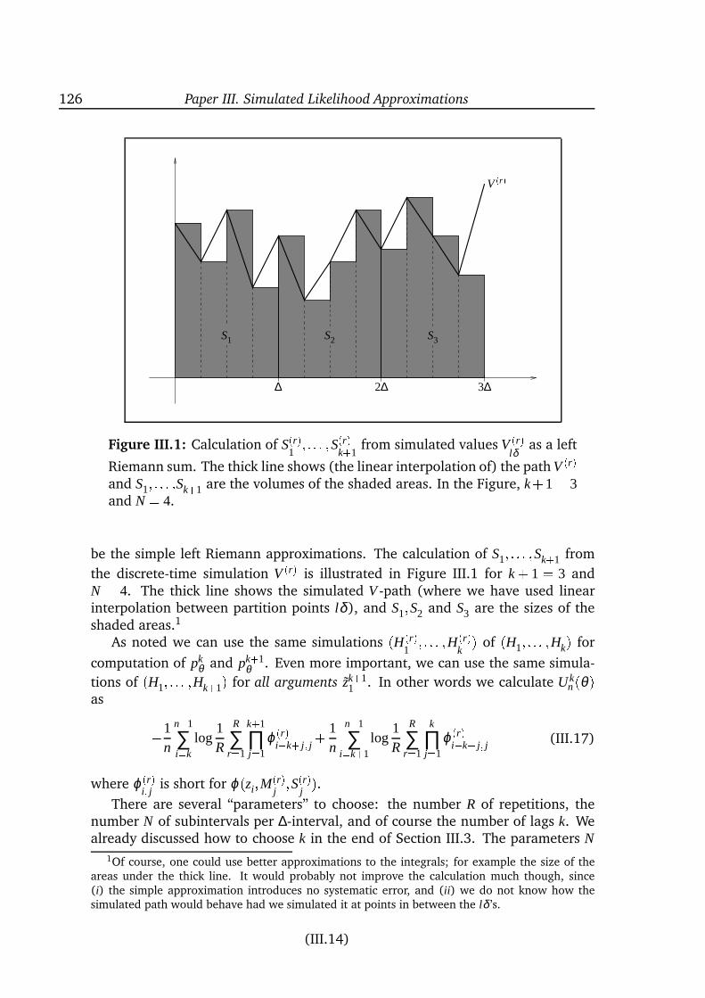
126 Paper III. Simulated Likelihood Approximations
S3
∆ 3∆2∆
V (r)S1 S2
Figure III.1: Calculation of S(r)1; : : : ;S(r)
k+1from simulated values V (r)
lδas a left
Riemann sum. The thick line shows (the linear interpolation of) the path V (r)and S1; : : : :Sk+1 are the volumes of the shaded areas. In the Figure, k+1= 3and N = 4.
be the simple left Riemann approximations. The calculation of S1; : : : ;Sk+1 from
the discrete-time simulation V (r) is illustrated in Figure III.1 for k + 1 = 3 andN = 4. The thick line shows the simulated V -path (where we have used linearinterpolation between partition points lδ), and S1;S2 and S3 are the sizes of theshaded areas.1
As noted we can use the same simulations (H(r)1; : : : ;H(r)
k) of (H1; : : : ;Hk) for
computation of pkθ and pk+1
θ . Even more important, we can use the same simula-
tions of (H1; : : : ;Hk+1) for all arguments zk+11 . In other words we calculate U k
n(θ)as 1
n
n1
∑i=k
log1R
R
∑r=1
k+1
∏j=1
ϕ(r)ik+ j; j + 1
n
n1
∑i=k+1
log1R
R
∑r=1
k
∏j=1
ϕ(r)ik+ j; j (III.17)
where ϕ(r)i; j is short for ϕ(zi;M(r)
j;S(r)
j).
There are several “parameters” to choose: the number R of repetitions, thenumber N of subintervals per ∆-interval, and of course the number of lags k. Wealready discussed how to choose k in the end of Section III.3. The parameters N
1Of course, one could use better approximations to the integrals; for example the size of theareas under the thick line. It would probably not improve the calculation much though, since(i) the simple approximation introduces no systematic error, and (ii) we do not know how thesimulated path would behave had we simulated it at points in between the lδ ’s.
(III.14)
III.5. Asymptotic results 127
and (in particular) R determine how accurately the values of U kn are determined
and must be large enough that the calculation of U kn (θ) is suitably stable, that is,
the simulated vales of U kn (θ) are “sufficiently close” for different simulations.
The number of calculations needed to compute one single value of U kn (θ) in-
creases approximately linearly in both R and k+1, and if computing time is lim-ited one must compromize between stability and the number of lags involved.Note that it might be necessary to increase R as k increases since we must simu-late longer paths of V and thus might need more simulations to obtain numericalstability.
So-called antithetic variables may increase computational stability. Here, itmeans that we make simulations of V in pairs where we in one simulation usethe randomly generated ε ’s in the Millstein scheme and in the other one use minus
the ε ’s. For R sets of randomly generated ε ’s we thus compute 2R simulated pathsof V , compute the ϕ(r)-values in (III.17) for each of the 2R simulated paths of V ,and average over all 2R simulations. The two ϕ(r)-values corresponding to thesame set of ε ’s (plus and minus) tend to be negatively correlated. The computingtime is approximately doubled when we use antithetic variables, but hopefully weneed R less than half as big as without antithetic variables in order to obtain sameprecision.
It is possible to compute suitably accurate values of U kn in reasonable time: for
n = 500 observations from the model where ξ 0 and V is a Cox-Ingersoll-Rossprocess, it takes somewhat less than a minute to compute a value of U4
n with N = 10and R = 10:000on a Digital alpha running at 500 MHz. This is only to give an ideaof the computational burden — no attempts have been made as to optimize theroutine.
Finally a very important remark: As always when criterion functions (or es-timating functions) are simulated, it is crucial to use the same random numbers
for different values of θ . Otherwise R must be chosen extremely large for thesimulated criterion function to behave continuously.
III.5 Asymptotic results
In this section we prove consistency and asymptotic normality (as n ! ∞) of theestimator θ k
n satisfying U kn(θ k
n ) = infθ2ΘU kn (θ). The results hold for any fixed values
of k and ∆. The true parameter is denoted by θ0, and all results are with respect toPθ0
.
It is essential for the results below that limit theorems hold for the sequenceZ. As already mentioned, the ergodic theorem holds under Assumption III.1 sinceα-mixing implies ergodicity. This, together with some regularity conditions, is suf-ficient to show consistency. For the asymptotic normality we furthermore needa central limit theorem for Z. We use a version of the central limit theorem in-volving further assumptions on the α-mixing coefficients. Both limit theorems areformulated and proved in the appendix (Theorem III.12) although the results arewell-known.
(III.15)
128 Paper III. Simulated Likelihood Approximations
The first term in (III.11) is negligible as n increases so we focus on the sum1n ∑n1
i=k+1 uc;kθ (zi+1jzi
ik+1). In the following we let jj jj denote the usual Eucledian
norm on Rp , and for a function g : Rp ! R and a probability Q on Rp we writeQ(g) for the integral
RgdQ.
III.5.1 Consistency
Apart from Assumption III.1 we need the following regularity conditions for con-sistency of θ k
n .
Assumption III.4 Fix k 0 and assume that the following conditions hold:
(B1) the parameter space Θ is a compact subset of Rp ;
(B2) for all θ 2 Θ there are a constant δθ > 0 and a function uθ : Rk+1 ! R in
L1(Pk+1θ0
) such that supθ 02Tθ ;δθ
uc;kθ 0 (zk+1jzk
1) uθ (zk+11 ) for all z1; : : : ;zk+1 2 R
where Tθ ;δ = fθ 0 2 Θ : jjθ θ 0jj δg;(B3) the functions θ ! uc;k
θ (zk+1jz1; : : : ;zk) from Θ to R are continuous for allz1; : : : ;zk+1 2 R;
(B4) the conditional distributions of Zk+1 given Zk1 = zk
1 with respect to Pk+1θ and
Pk+1θ 0 are different for θ 6= θ 0 and all z1; : : : ;zk 2 R.
Note that conditions (B1) and (B3) ensure that a minimum of U kn exists, but
the minimum could be attained at the boundary of Θ and need not be unique.Condition (B2) expresses that uc;k
θ is locally dominated integrable wrt. Pk+1θ0
and
implies that uc;kθ is in L1(Pk+1
θ0) for all θ 2 Θ. The ergodic theorem thus yields
U kn (θ)! Pk+1
θ0(uc;k
θ ) = Eθ0uc;k
θZk+1jZ1; : : : ;Zk
(III.18)
as n!∞ in Pθ0-probability (even Pθ0
-a.s and in L1(Pθ0)). Denote the limit by Jk(θ).
Conditions (B2) and (B3) make U kn and Jk continuous and ensure that the conver-
gence (III.18) holds uniformly in θ (Lemma III.6). Condition (B4) is an identifia-bility condition ensuring that Jk has unique minimum for θ = θ0 as asserted in thefollowing lemma.
Lemma III.5 Assume that Assumption III.1 holds. If furthermore (B2) and (B4)
hold then Jk(θ) Jk(θ0) for all θ 2Θ with equality if and only if θ = θ0.
(III.16)
III.5. Asymptotic results 129
Proof By definition of Jk and Jensen’s inequality we get for θ 2 Θ
Jk(θ0) Jk(θ) = Eθ0uc;k
θ0(Zk+1jZk
1)Eθ0uc;k
θ (Zk+1jZk1)= Eθ0
log
pc;kθ (Zk+1jZk
1)pc;k
θ0(Zk+1jZk
1) logEθ0
pc;kθ (Zk+1jZk
1)pc;k
θ0(Zk+1jZk
1)with equality if and only if pc;k
θ (zk+1jzk1) = pc;k
θ0(zk+1jzk
1) for Pθ0-almost all z1; : : : ;zk+1,
that is, if and only if θ = θ0 by condition (B4). The density of (Z1; : : : ;Zk+1) wrt.
Pθ0at (z1; : : : ;zk+1) is pk
θ0(zk
1)pc;kθ0(zk+1jzk
1). Hence,
Eθ0
pc;kθ (Zk+1jZk
1)pc;k
θ0(Zk+1jZk
1)= ZRk+1pc;k
θ (zk+1jzk1) pk
θ0(zk
1)d(zk+11 )= ZRk
pkθ0(zk
1)ZR pc;kθ (zk+1jzk
1)dzk+1 dzk1= ZRk
pkθ0(zk
1)dzk1= 1
where we have used that pc;kθ (jzk
1) and pkθ0() are densities on R and Rk respectively.
It follows that Jk(θ0) Jk(θ) log1= 0 with equality if and only if θ = θ0. The next lemma claims that the convergence (III.18) is uniform in θ 2 Θ. It is
of course important that Θ is compact. The proof is almost identical to the proofof Lemma 3.3 in Bibby & Sørensen (1995) but is given here for completeness.
Lemma III.6 Under Assumption III.1 and conditions (B1), (B2), and (B3), Jk is
continuous and supθ2ΘU k
n (θ) Jk(θ)! 0 as n!∞ in probability wrt. Pθ0.
Proof We first show continuity of Jk: Let θn ! θ and choose δθ and uθ according
to (B2). Then jjθnθ jj< δθ and henceuc;k
θn
uθ for n large enough. Dominated
convergence now yields Jk(θn)! Jk(θ).Next, recall that Tθ ;δ = fθ 0 2 Θ : jjθ θ 0jj δg and define the function w :
Θ (0;∞)Rk+1 by
w(θ ;δ ;zk+11 ) = sup
θ 02Tθ ;δ uc;kθ (zk+1jzk
1)uc;kθ 0 (zk+1jzk
1):Then w(θ ;δ ;zk+1
1 )! 0 as δ ! 0 for all θ 2 Θ and all z1; : : : ;zk+1 2 R. This follows
from condition (B3) on continuity of θ ! uc;kθ (zk+1jzk
1). Also, w(θ ;δ ; ) is dominated
(III.17)
130 Paper III. Simulated Likelihood Approximations
by 2uθ for all θ 2 Θ, all δ < δθ and all z1; : : : ;zk+1 2 R. Of course δθ and uθ arechosen according to condition (B2). Hence, by dominated convergence w(θ ;δ ; )is in L1(Pk+1
θ0) for δ < δθ and Eθ0
w(θ ;δ ;Zk+11 )! 0 as δ ! 0 for all θ 2 Θ.
Now let ε > 0. For each θ 2 Θ choose λθ 2 (0;δθ such that w(θ ;δ ; ) is in
L1(Pk+1θ0
) with Eθ0w(θ ;δ ;Zk+1
1 ) < ε=4 for all δ < δθ and jJk(θ) Jk(θ 0)j < ε=4 ifjjθθ 0jj< λθ (recall that Jk is continuous). Let B(θ ;λ ) = fθ 0 2 Rp : jjθ θ 0jj< λgbe the ball with centre θ and radius λ . Then Θ [θ2ΘB(θ ;λθ ) and since Θ iscompact the open covering of Θ has a finite sub-covering. That is, θ1; : : : ;θm existsuch that Θ [m
j=1B(θ j;λθ j).
Consider a fixed θ 2Θ and choose j 2 f1; : : : ;mg such that θ 2 B(θ j;λθ j). Thenjjθ θ jjj< λθ j
andU kn (θ) Jk(θ) U k
n (θ j) Jk(θ j)+ U kn (θ)U k
n(θ j)+ Jk(θ j) Jk(θ):Here, the first term only depends on θ j and the third term is smaller than ε=4. Forthe second term, note thatU k
n (θ)U kn (θ j)= 1n n1
∑i=k+1
uc;k
θ (Zi+1jZiik+1)uc;k
θ j(Zi+1jZi
ik+1) 1n
n1
∑i=k+1
uc;kθ (Zi+1jZi
ik+1)uc;kθ j(Zi+1jZi
ik+1) 1n
n1
∑i=k+1
wθ j;λθ j
;Zi+1ik+1
1n
n1
∑i=k+1
wθ j;λθ j
;Zi+1ik+1
Eθ0wθ j;λθ j
;Zk+11
+ ε=4
which only depends on θ j. It follows that the supremum of jU kn (θ)Jk(θ)j over Θ
is bounded by the maximum over fθ1; : : : ;θmg:supθ2Θ
U kn (θ) Jk(θ) max
j=1;::: ;mU kn (θ j) Jk(θ j)+ max
j=1;::: ;m1n n1
∑i=k+1
wθ j;λθ j
;Zi+1ik+1
Eθ0wθ j;λθ j
;Zk+11
+ ε=2:Recall that λθ j
is chosen such that w(θ j;λθ j) is in L1(Pk+1
θ0). Also, uc;k
θ jis in L1(Pk+1
θ0)
by condition (B2). Hence, by the ergodic theorem, the two first terms converge tozero in Pθ0
-probability and the lemma follows immediately. With these lemmas in hand it is easy to prove consistency of θ k
n :
Theorem III.7 Under Assumptions III.1 and III.4, θ kn is consistent for θ0, that is,
θ kn ! θ0 in probability wrt. Pθ0
as n! ∞.
(III.18)
III.5. Asymptotic results 131
Proof By assumption, Θ is compact and θ !U kn (θ) is continuous. The function Jk
is well-defined under (B2) and continuous under (B3), see Lemma III.6. Since Jk
is defined on a compact set Jk is even uniformly continuous.
For η > 0 define Wn(η) = supjjθθ 0jjηU k
n (θ)U kn (θ 0). Then θ k
n is consistent if
Pθ0
Wn(η) 2ψ(η)! 0; n! ∞ (III.19)
where ψ : [0;∞)! R satisfies limη!0 ψ(η) = 0 (Dacunha-Castelle & Duflo 1986,
Theorem 3.2.8).
By the triangle inequality
Wn(η) supjjθθ 0jjη
U kn (θ) Jk(θ)+ Jk(θ) Jk(θ 0)+ U k
n (θ 0) Jk(θ 0) 2 supθ2Θ
U kn(θ) Jk(θ)+ supjjθθ 0jjη
Jk(θ) Jk(θ 0):Here, the first term converges to zero in Pθ0
-probability, cf. Lemma III.6 above. The
second term is deterministic and converges to zero as η ! 0 since Jk is uniformlycontinuous. Hence, with ψ(η) = supjjθθ 0jjη
Jk(θ) Jk(θ 0), condition (III.19)
and thus consistency of θ kn follows.
III.5.2 Asymptotic normality
We now turn to asymptotic normality of θ kn . Assume that the criterion function
U kn is continuously differentiable (Assumption (C2) below) and let U k
n denote thep-vector of first derivatives. Then any minimizer of U k
n is either on the boundaryof Θ or solves the equation U k
n (θ) = 0. In the latter case the theory of estimat-ing functions applies, see Sørensen (1998b), for example. Theorem III.9 belowclaims that (with a probability tending to one) there exists a solution to U k
n (θ) = 0and that the solution is asymptotically normal. Let us be more specific about theregularity conditions:
Assumption III.8 Let ΘÆ denote the set of inner points of Θ and assume that
(C1) the true parameter θ0 is an inner point of Θ, i.e. θ0 2ΘÆ;(C2) the functions θ ! pc;k
θ (zk+1jzk1) are twice continuously differentiable for all
z1; : : : ;zk+1 2 R.
Then θ ! uc;kθ (zk+1jzk
1) is twice continuously differentiable as well. Let uc;kθ =(uc;k
θ ; j) j=1;::: ;p = (∂θ juc;k
θ ) j=1;::: ;p denote the p-vector of first derivatives and let uc;kθ =(uc;k
θ ; jl) j;l=1;::: ;p = (∂θ j∂θl
uc;kθ ) j;l=1;::: ;p be the symmetric p p-matrix of second deriv-
atives of uc;kθ . Assume furthermore that
(III.19)
132 Paper III. Simulated Likelihood Approximations
(C3) there exists an η > 0 such that uc;kθ0; j is in L2+η (Pk+1
θ0) for all j = 1; : : : ; p
and such that the α-mixing coefficients for Z corresponding to θ0 satisfy
∑∞m=1αZ(m)2=(2+η) < ∞;
(C4) there is a neighbourhood T0 of θ0 such that for all θ 2 T0 and all j; l = 1; : : : ; pthere is a constant δθ ; jl > 0 and a function uθ ; jl : Rk+1 ! R in L1(Pk+1
θ0) such
that for all z1; : : : ;zk+1 2 R, supθ 02Tθ ;δθ ; jl
uc;kθ 0; jl(zk+1jzk
1) uθ ; jl(zk+11 ) where, as
before, Tθ ;δ = fθ 0 2 Θ : jjθ θ 0jj δg;(C5) the symmetric p p matrix
Ak(θ0) = Pk+1θ0
uc;k
θ0
= Eθ0uc;k
θ0(Zk+1jZk
1)is positive definite.
Under (C2), U kn is twice continuously differentiable with first derivative given
by the p-vector U kn (θ) = 1
n ∑n1i=k+1 uc;k
θ (zi+1jziik+1) and second derivative given by
the p p matrix U kn = 1
n ∑n1i=k+1 uc;k
θ (zi+1jxiik+1). Any minimizer of U k
n is either on
the boundary of Θ or solves U kn(θ) = 0. In particular, under (C1), any minimizer
of U kn that is consistent for θ0 solves the estimating equation (with a probability
tending to one).Note that the estimating function U k
n is unbiased, that is, Eθ U kn(θ) = 0 for all
θ 2 ΘÆ. Indeed,
Eθ uc;kθ ; j(Zk+1jZk
1) = Eθ Eθ
uc;k
θ ; j(Zk+1jZk1)Zk
1
and, with obvious notation for the derivatives of pc;k
θ (and if differentiation wrt. θ jand integration wrt. zk+1 are interchangeable),
Eθ
uc;k
θ ; j(Zk+1)Zk1 = zk
1
=Zpc;k
θ ; j(zjzk1)dz = ∂
∂θ j
Zpc;k
θ (zjzk1)dz = 0
for all z1; : : : ;zk 2 R and all j = 1; : : : ; p.It is essential for the proof below that the estimating function itself evaluated
at the true parameter value and scaled by n1=2 converges in distribution. Un-der condition (C3) this follows from the central limit theorem for α-mixing pro-cesses in the appendix (Theorem III.12.2). To be specific let ζ j(zi+1
ik+1) be short
for uc;kθ0; j(zi+1jzi
ik+1); then Theorem III.12.2 claims that the p p matrix Γk defined
coordinate-wise by
Γkjl(θ0) = Eθ0
ζ j(Zk+1
1 )ζl(Zk+11 )+ ∞
∑m=1
nEθ0
ζ j(Zk+1
1 )ζl(Zk+m+1m+1 )+Eθ0
ζl(Zk+1
1 )ζ j(Zk+m+1m+1 )o
(III.20)
III.5. Asymptotic results 133
is well-defined and that n1=2U kn (θ0)! N(0;Γk(θ0)).
Condition (C4) ensures integrability of uc;kθ0
and suitably uniform convergence
in probability of U kn (θ0) to Ak(θ0). Note that if integration and twice differentiation
can be interchanged, then Pk+1θ0
(pc;kθ0=pc;k
θ0) = 0 and
Ak(θ0) = Pk+1θ0
uc;k
θ0
= Pk+1θ0
uc;k
θ0
uc;k
θ0
T;
that is, Ak(θ0) equals the first term in Γk. The condition that Ak(θ0) is positivedefinite is an identifiability condition.
Theorem III.9 Suppose that Assumptions III.1 and III.8 hold. Then a solution θ kn to
U kn (θ) = 0 exists with a probability tending to 1 as n! ∞. Moreoverp
nθ k
n θ0
! NAk(θ0)1Γk(θ0)Ak(θ0)1: (III.20)
Proof It follows from Corollary 2.5 and Theorem 2.8 in Sørensen (1998b) that itis sufficient to show
n1=2U kn (θ0)! N
0;Γk(θ0) (III.21)
in distribution wrt. Pθ0as n! ∞ and
supθ2Tθ0;η=pn
U kn; jl(θ)Ak(θ0)! 0 (III.22)
in probability wrt. Pθ0as n! ∞ for all η > 0 and all j; l 2 f1; : : : ; pg.
As already noted (III.21) follows immediately from condition (C3) and Theo-rem III.12.2. In order to show (III.22) define Ak(θ) = Pk+1
θ0
uc;k
θ
for θ 2 T0 and let
j; l 2 f1; : : : ; pg and η > 0 be fixed. By the triangle inequalityU kn; jl(θ)Ak(θ0) U k
n; jl(θ)Ak(θ)+ Ak(θ)Ak(θ0):Choose N large enough that Tθ0;η=pN
T0. Then, for n N, Ak(θ) is well-defined
for all θ 2 Tθ0;η=pn. By arguments almost identical to those in the proof of Theo-
rem III.6 it now follows that
supθ2Tθ0;η=pN
U kn; jl(θ)Ak(θ)! 0
in Pθ0-probability as n! ∞ (recall that Tθ0;η=pN
is compact).
Also, Ak is continuous in θ0. The convergence (III.22) follows immediately.This proves both the existence assertion and the convergence result (III.20).
(III.21)
134 Paper III. Simulated Likelihood Approximations
Note that although asymptotic normality is indeed a nice property of the esti-mator, it is difficult to use in practice as we are not able to compute the asymptoticvariance. Also, the above conditions are all expressed in terms of the distributionof Z and are thus in general difficult (if possible at all) to check. The conditionon the α-mixing coefficients in (C3) is an exception: we showed in the proofof Proposition III.2 that αZ( j) αV
( j 1)∆ for all j 2 so it is sufficient thatthe condition holds for the α-mixing coefficients for V . See Genon-Catalot et al.
(1998b), for example, for conditions ensuring exponential decay of the α-mixingcoefficients for V .
Recall from (III.14) that for ξ 0 and k = 0, the identifiability condition (B4)holds if and only if the distributions of S1 corresponding to two values θ and θ 0differ when θ 6= θ 0. We have no similar results for larger values of k. For theremaining conditions recall that
uc;kθ (zk+1jzk
1) = logEπk+1θ
k+1
∏i=1
ϕ(zi;Hi)+ logEπkθ
k
∏i=1
ϕ(zi;Hi)where Hi = (Mi;Si), π l
θ is the distribution of H l = (H1; : : : ;Hl) and ϕ(;h) = ϕ(;m;s)is the density of N(m;s) for h = (m;s). Hence, the continuity, differentiability andlocal integrability conditions imposed on uc;k
θ would follow from roughly similar
conditions on the densities of Hk1 and Hk+1
1 . This is not very helpful though, sincewe have no explicit expression for the latter densities either.
Finally, it is important to stress that the above results hold for fixed value ofk (and ∆) as n ! ∞. In particular, the above results do not imply nice asymptoticbehaviour of the maximum likelihood estimator (which corresponds to k = k(n) =n1). The problem is of course that the terms in the log-likelihood function Un1
noriginate from different functions (pc;i
θ for observation zi+1) such that the usual
limit theorems do not apply.As noted in Section III.2 we can think of the model as a hidden Markov model
with continuous, unbounded state space of the hidden chain H given by Hi =(Vi∆;Mi;Si). Asymptotic results for the maximum likelihood estimator have beenproved for hidden Markov models where the state space for the hidden chain isfinite (Bickel & Ritov 1996, Bickel, Ritov & Rydén 1998) or compact (Jensen &Petersen 1999). Neither approach can be applied in our setting and there are infact no results in the literature concerning asymptotic properties of the maximumlikelihood estimator for the models considered in this paper.
III.6 Efficiency considerations
In this section we briefly discuss how the number of lags k influence the quality ofthe estimators. The subject is essential but unfortunately we have not been ableto prove very powerful results.
Intuitively we would expect estimators to improve as the number of lags in-creases. With the asymptotic normality from Theorem III.9 in hand we could
(III.22)
III.6. Efficiency considerations 135
compare estimators for different k’s by their asymptotic variances and hope thatthe variance is decreasing as a function of k (for symmetric positive semi-definitematrices A and B we write A B if and only if the difference BA is positive semi-definite). We have not been able to prove results like this! The problem is of coursethat the expression for the asymptotic variance is so complicated that comparisonbetween different k’s is impossible, even for a one-dimensional parameter.
The simulation study in Section III.7 indicates that minimization of U kn in prac-
tice may give rise to identification problems even if the k-lag conditional distribu-tion uniquely determines the parameter (theoretically). In the simulation studythis is reflected in very oblong level curves corresponding to small values of cer-tain linear combinations of the coordinates in Eθ0
U kn (θ0) and thereby (ignoring the
matrix Γ(θ0) in (III.20)) to large asymptotic variance of the estimator. In the simu-lation study the problem seems to diminish as we use larger values of k suggestingthat estimation in fact improves as k increases. On the other hand, in a simplersituation with no identification problems for any value of k we did not find anysubstantial differences among the estimators for different values of k.
Note that we in principle could improve estimation by introducing weight func-tions. To be specific, consider estimating functions on the form
Dkn(θ) = 1
n
n1
∑i=k
di(Ziik+1;θ) uc;k
θ (Zi+1jZiik+1)
where dk; : : : ;dn1 are function from Rk Θ to R. Note that we for simplicity have
left out the contribution from the first k observations and that U kn (except for the
first term in U kn ) corresponds to di 1, i = k; : : : ;n1.
The estimating function Dkn is unbiased since for each i = k : : : ;n1
Eθ0di(Zi
ik+1;θ0)uc;kθ0(Zi+1jZi
ik+1)= Eθ0di(Zi
ik+1)Eθ0uc;k
θ0(Zi+1jZi
ik+1)jZiik+1
= 0:Under regularity conditions similar to those of Assumption III.8 the solution toDk
n(θ) = 0 is a consistent and asymptotically normal estimator of θ . By choosingthe functions di cleverly we can obtain smaller asymptotic variance than is the case
for θ kn , see Sørensen (1999) for similar considerations. This is only of theoretical
interest, though! In order to find the optimal weight functions one must invert an(n k) (n k) matrix (which depends on θ and whose entries we do not evenknow explicitly).
Finally, we prove a result concerning the approximate log-likelihood functionsU k
n rather than the corresponding estimators: the limit, in probability, of U kn (θ0) is
decreasing in k. It holds only for U kn evaluated at the true parameter and is thus
not very useful in practice. Nevertheless it tells us that the approximations of thelikelihood improve in this sense.
(III.23)
136 Paper III. Simulated Likelihood Approximations
Proposition III.10 Let 0 k0 k00 and assume that Condition (B2) is satisfied for
θ = θ0 and k = k0 and k = k00. Then
Eθ0uc;k00
θ0
Zk00+1jZk00
1
Eθ0uc;k0
θ0
Zk0+1jZk0
1
:Consequently, Eθ0
U k00n (θ0) Eθ0
U k0n (θ0) and limn!∞U k00
n (θ0) limn!∞U k0n (θ0) where
convergence means convergence in Pθ0-probability.
Proof It will suffice to consider k0 = k and k00 = k+1 for k 0 arbitrary. By station-arity it follows that it is sufficient to show that
Eθ0uc;k+1
θ0
Zk+2jZk+1
1
Eθ0uc;k
θ0
Zk+2jZk+1
2
: (III.23)
By definition,
uc;k+1θ0
Zk+2jZk+1
1
uc;kθ0
Zk+1jZk
1
= logpc;k
θ0
Zk+2jZk+1
2
pc;k+1
θ0
Zk+2jZk+1
1
so Jensen’s equality yields
Eθ0
uc;k+1
θ0
Zk+2jZk+1
1
uc;kθ0
Zk+2jZk+1
2
logEθ0
pc;kθ0
Zk+2jZk+1
2
pc;k+1
θ0
Zk+2jZk+1
1
:Calculations similar to those in the proof of Lemma III.5 show that the latter expec-tation is one, which yields (III.23). The expectation assertion follows immediatelyby
U k+1n (θ0)U k
n (θ0) = 1n
n1
∑k=1
uc;k+1
θ0
Zi+1jZi
ik
uc;kθ0
Zi+1jZi
ik+1
and the convergence result follows by the ergodic theorem. III.7 Example: The Cox-Ingersoll-Ross process
In this section we discuss a particular model, namely the model where the ob-served X -process has no drift, and the volatility process V is a Cox-Ingersoll-Ross
process. This specification of the volatility process was first considered by Hull &White (1987) and later by Heston (1993).
III.7.1 Basic properties
The model is given by the stochastic differential equations
dXt =pVt dWt ; X0 =UX
dVt = α(β Vt)dt +σp
Vt dWt ; V0 =UV :(III.24)
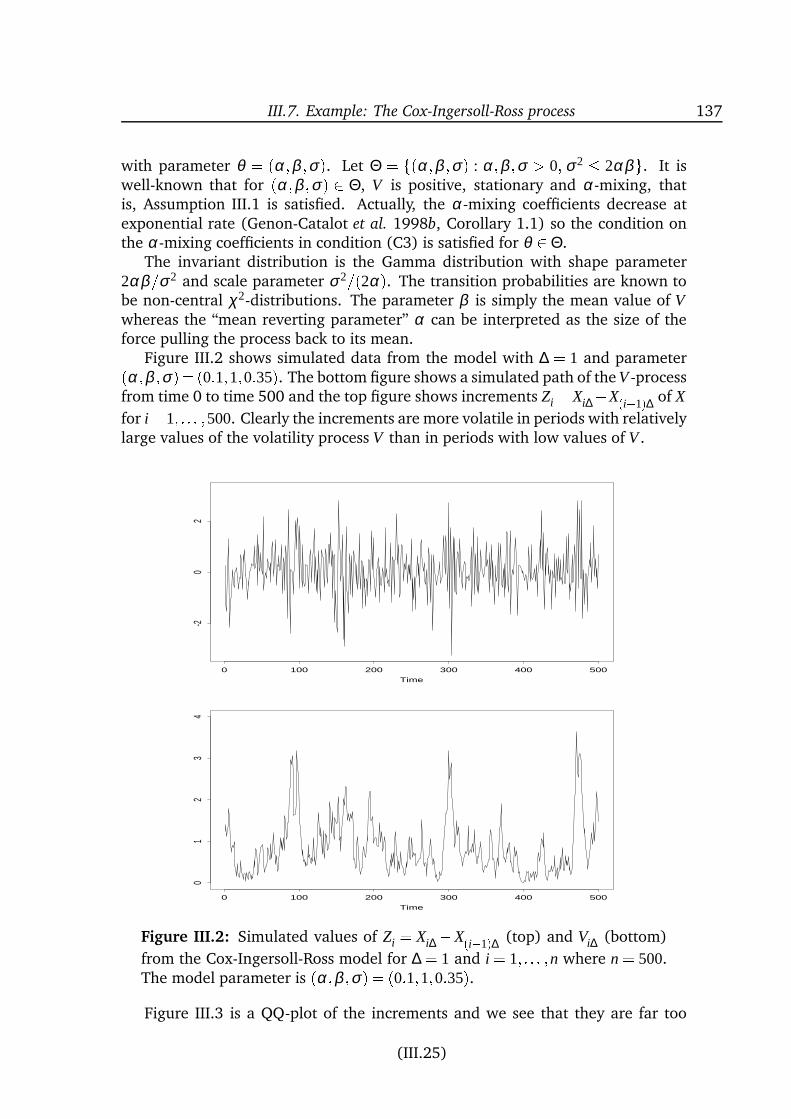
III.7. Example: The Cox-Ingersoll-Ross process 137
with parameter θ = (α;β ;σ). Let Θ = f(α;β ;σ) : α;β ;σ > 0; σ2 2αβg. It iswell-known that for (α;β ;σ) 2 Θ, V is positive, stationary and α-mixing, thatis, Assumption III.1 is satisfied. Actually, the α-mixing coefficients decrease atexponential rate (Genon-Catalot et al. 1998b, Corollary 1.1) so the condition onthe α-mixing coefficients in condition (C3) is satisfied for θ 2 Θ.
The invariant distribution is the Gamma distribution with shape parameter2αβ=σ2 and scale parameter σ2=(2α). The transition probabilities are known tobe non-central χ2-distributions. The parameter β is simply the mean value of Vwhereas the “mean reverting parameter” α can be interpreted as the size of theforce pulling the process back to its mean.
Figure III.2 shows simulated data from the model with ∆ = 1 and parameter(α;β ;σ)= (0:1;1;0:35). The bottom figure shows a simulated path of the V -processfrom time 0 to time 500 and the top figure shows increments Zi = Xi∆X(i1)∆ of X
for i= 1; : : : ;500. Clearly the increments are more volatile in periods with relativelylarge values of the volatility process V than in periods with low values of V .
Time
0 100 200 300 400 500
-20
2
Time
0 100 200 300 400 500
01
23
4
Figure III.2: Simulated values of Zi = Xi∆X(i1)∆ (top) and Vi∆ (bottom)
from the Cox-Ingersoll-Ross model for ∆ = 1 and i = 1; : : : ;n where n = 500.The model parameter is (α;β ;σ) = (0:1;1;0:35).Figure III.3 is a QQ-plot of the increments and we see that they are far too
(III.25)
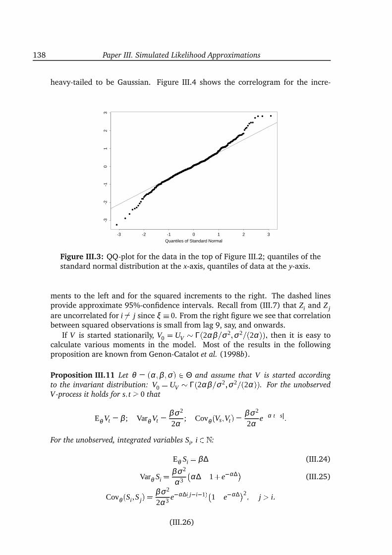
138 Paper III. Simulated Likelihood Approximations
heavy-tailed to be Gaussian. Figure III.4 shows the correlogram for the incre-
Quantiles of Standard Normal
-3 -2 -1 0 1 2 3
-3-2
-10
12
3
Figure III.3: QQ-plot for the data in the top of Figure III.2; quantiles of thestandard normal distribution at the x-axis, quantiles of data at the y-axis.
ments to the left and for the squared increments to the right. The dashed linesprovide approximate 95%-confidence intervals. Recall from (III.7) that Zi and Z jare uncorrelated for i 6= j since ξ 0. From the right figure we see that correlationbetween squared observations is small from lag 9, say, and onwards.
If V is started stationarily, V0 = UV Γ(2αβ=σ2;σ2=(2α)); then it is easy tocalculate various moments in the model. Most of the results in the followingproposition are known from Genon-Catalot et al. (1998b).
Proposition III.11 Let θ = (α;β ;σ) 2 Θ and assume that V is started according
to the invariant distribution: V0 = UV Γ(2αβ=σ2;σ2=(2α)). For the unobserved
V -process it holds for s; t 0 that
Eθ Vt = β ; Varθ Vt = βσ2
2α; Covθ (Vs;Vt) = βσ2
2αeαjtsj:
For the unobserved, integrated variables Si, i 2 N:
Eθ Si = β∆ (III.24)
Varθ Si = βσ2
α3
α∆1+ eα∆ (III.25)
Covθ (Si;S j) = βσ2
2α3 eα∆( ji1)1 eα∆2; j > i:(III.26)
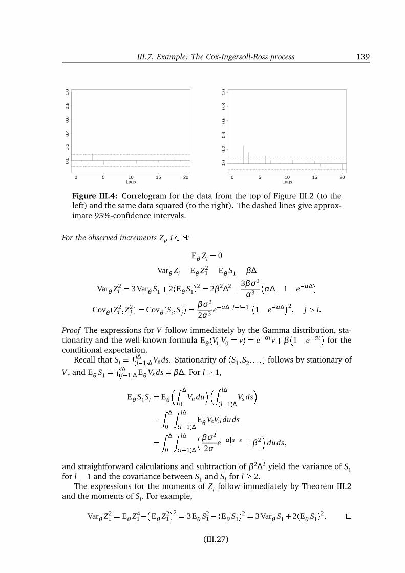
III.7. Example: The Cox-Ingersoll-Ross process 139
Lags0 5 10 15 20
0.0
0.2
0.4
0.6
0.8
1.0
Lags0 5 10 15 20
0.0
0.2
0.4
0.6
0.8
1.0
Figure III.4: Correlogram for the data from the top of Figure III.2 (to theleft) and the same data squared (to the right). The dashed lines give approx-imate 95%-confidence intervals.
For the observed increments Zi, i 2 N:
Eθ Zi = 0
Varθ Zi = Eθ Z21 = Eθ S1 = β∆
Varθ Z2i = 3Varθ S1+2(Eθ S1)2 = 2β 2∆2+ 3βσ2
α3
α∆1+ eα∆
Covθ (Z2i ;Z2
j ) = Covθ (Si;S j) = βσ2
2α3 eα∆( ji1)1 eα∆2; j > i:Proof The expressions for V follow immediately by the Gamma distribution, sta-tionarity and the well-known formula Eθ (VtjV0 = v) = eαtv+β
1 eαt
for the
conditional expectation.Recall that Si = R i∆(i1)∆Vs ds. Stationarity of (S1;S2; : : :) follows by stationary of
V , and Eθ S1 = R i∆(i1)∆ Eθ Vs ds = β∆. For l 1,
Eθ S1Sl = Eθ
Z ∆
0Vu du
Z l∆(l1)∆Vs ds= Z ∆
0
Z l∆(l1)∆ Eθ VsVu duds= Z ∆
0
Z l∆(l1)∆βσ2
2αeαjusj+β 2
duds;
and straightforward calculations and subtraction of β 2∆2 yield the variance of S1for l = 1 and the covariance between S1 and Sl for l 2.
The expressions for the moments of Zi follow immediately by Theorem III.2and the moments of Si. For example,
Varθ Z21 = Eθ Z4
1Eθ Z21
2 = 3Eθ S21 (Eθ S1)2 = 3Varθ S1+2(Eθ S1)2:
(III.27)
140 Paper III. Simulated Likelihood Approximations
Note that Varθ Z21 > 3Varθ S1 and that Covθ (Z2
1;Z2j ) = Covθ (S1;S j) > 0 is de-
creasing at exponential rate. The correlation between Z21 and Z2
j is thus positive,exponentially decreasing and at most 1/3 for all j 2. In fact it is at most 1/5which can be seen as follows:
Corrθ (Z21;Z2
j ) = σ21 eα∆2
4α3β∆2+6σ2α∆1+ eα∆
eα∆( j2)which is increasing in σ2. For fixed α and β , the correlation is hence maximal forσ2 = 2αβ , with
Corr(α;β ;(2αβ )1=2)(Z21;Z2
j ) = 1 eα∆2
2α2∆2+6α∆1+ eα∆
eα∆( j2):The right hand side does not depend on β and is decreasing as a function of α∆with limit 1/5 as α∆ ! 0. Also note that the excess kurtosis Eθ Z4
1=(Eθ Z21)23 is
at most 3. Hence, the model is not appropriate for data with very heavy tails orwith large correlations between squared observations Z2
1 and Z2j for some j 2.
III.7.2 A small simulation study
In the following we present a small simulation study. We have simulated 10datasets of increments, Z1; : : : ;Z10, each consisting of n = 500 observations. Themodel parameters are (α;β ;σ) = (α0;β0;σ0) = (0:1;1;0:35)and the value of ∆ is 1. Each dataset was simulated as follows: a V -processwas simulated by the Millstein scheme with each interval [(i 1)∆; i∆ split into1000 subintervals; the integrals S1; : : : ;Sn were approximated as described in Sec-tion III.4; and Z1; : : : ;Zn were finally drawn independently, Zi from N(0;Si). Oneof the simulated datasets, Z4, was shown in Figure III.2 together with the corre-sponding simulated V -values, and we shall use this dataset as example throughoutthe section.
In a real-world application we would not have observed the V -process at all,but in this simulation study we have saved the simulated values V0;V∆; : : : ;Vn∆ foreach simulation. Hence, we can estimate the parameters from the V -process aswell as from the Z’s and thus get an idea of how much information is lost when Zrather than V is observed (see comments below).
By Proposition III.11 it is easy to calculate various moments of V , S and Z forthe chosen values of α;β ;σ and ∆. For example,
Eθ0V0 = 1; Varθ0
V0 = 0:613; Corrθ0(V0;V∆) = 0:905
Eθ0S1 = 1; Varθ0
S1 = 0:593; Corrθ0(S1;S2) = 0:936
Varθ0Z1 = Eθ0
Z21 = 1; Eθ0
Z41 = 4:778; Corrθ0
(Z21;Z2
2) = 0:147:(III.28)
III.7. Example: The Cox-Ingersoll-Ross process 141
We see that values of V at two consecutive time points (i1)∆ and i∆ as well astwo consecutive S’s are strongly correlated, and that the excess kurtosis of Z is1.778.
For later use, define m2(θ) = Eθ Z21, m4(θ) = Eθ Z4
1 and m1;2(θ) = Eθ Z21Z2
2 andlet for a given dataset
m2 = 1n
n
∑i=1
Z2i ; m4 = 1
n
n
∑i=1
Z4i ; m1;2 = 1
n1
n
∑i=2
Z2i1Z2
i
be the corresponding empirical moments. Also, let c1;2 = (m1;2 m22)=(m4 m2
2) bethe first empirical autocorrelation coefficient. Table III.1 in Appendix III.B lists theaverage and m2, m4, m1;2 and c1;2 for the simulated datasets.
In the rest of this section we shall estimate the parameters α, β and σ fromeach of the ten simulated datasets. We consider three different set-ups; (A) onlyone parameter, say α, is considered unknown whereas the two others are known;(B) two parameters are considered unknown; (C) all three parameters are consid-ered unknown. Cases (A) and (B) are of course not realistic but provide insight tothe estimation problem.
In case (A) we compute the estimators αkn for k = 0; : : : ;4 although it turns out
that even k = 0 yields satisfactory estimates. A comparison of the five values of kwith respect to mean and variance (over the ten simulations) shows that k = 1 isthe best choice and k = 0 the worst, but the difference between the five estimatorsis not substantial. In case (B) we use only k = 0 and k = 1; both values yieldacceptable estimates as long as β is not the unknown parameter. The estimationproblem in case (C) is more difficult, and we must use larger values of k, say k = 4.Still, the estimators are not completely satisfactory.
In each of the three cases we compare (i) with “method of moments estimators”(Genon-Catalot et al. 1998b), that is, estimators obtained by matching variousempirical and theoretical moments; and (ii) with simple martingale estimatorsbased on the V -data (Bibby & Sørensen 1995, Sørensen 1997). The latter wouldof course not be possible in practice. The moment estimators are quite bad andthere are often existence problems. The estimators based on V are not surprisinglyquite good. In case (A) the difference between the estimators based on V and theapproximate maximum likelihood estimators based on Z is moderate, whereas itis very substantial in case (C)
Of course, the above results are only indications of the relations between theestimators. We cannot draw final conclusions from the simulation study, since itis based on only ten simulations. However, the study confirms that the method isindeed applicable in practice!
Now, let us go through the three cases in detail. For all the below computationsof U k
n we have used N = 10 and R = 10:000, cf. Section III.4. We start out gentlyand consider estimation of one parameter only.
(III.29)
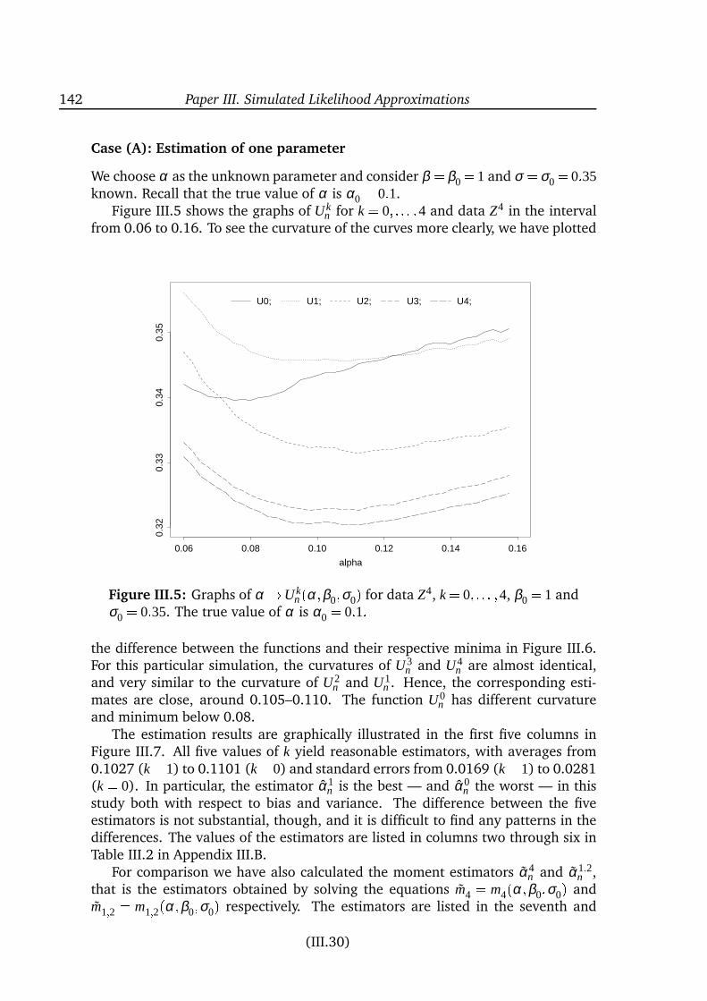
142 Paper III. Simulated Likelihood Approximations
Case (A): Estimation of one parameter
We choose α as the unknown parameter and consider β = β0 = 1 and σ =σ0 = 0:35known. Recall that the true value of α is α0 = 0:1.
Figure III.5 shows the graphs of U kn for k = 0; : : : ;4 and data Z4 in the interval
from 0.06 to 0.16. To see the curvature of the curves more clearly, we have plotted
alpha
0.06 0.08 0.10 0.12 0.14 0.16
0.32
0.33
0.34
0.35
U0; U1; U2; U3; U4;
Figure III.5: Graphs of α !U kn(α;β0;σ0) for data Z4, k = 0; : : : ;4, β0 = 1 and
σ0 = 0:35. The true value of α is α0 = 0:1:the difference between the functions and their respective minima in Figure III.6.For this particular simulation, the curvatures of U3
n and U4n are almost identical,
and very similar to the curvature of U2n and U1
n . Hence, the corresponding esti-mates are close, around 0.105–0.110. The function U0
n has different curvatureand minimum below 0.08.
The estimation results are graphically illustrated in the first five columns inFigure III.7. All five values of k yield reasonable estimators, with averages from0.1027 (k = 1) to 0.1101 (k = 0) and standard errors from 0.0169 (k = 1) to 0.0281(k = 0). In particular, the estimator α1
n is the best — and α0n the worst — in this
study both with respect to bias and variance. The difference between the fiveestimators is not substantial, though, and it is difficult to find any patterns in thedifferences. The values of the estimators are listed in columns two through six inTable III.2 in Appendix III.B.
For comparison we have also calculated the moment estimators α4n and α1;2
n ,that is the estimators obtained by solving the equations m4 = m4(α;β0;σ0) andm1;2 = m1;2(α;β0;σ0) respectively. The estimators are listed in the seventh and
(III.30)
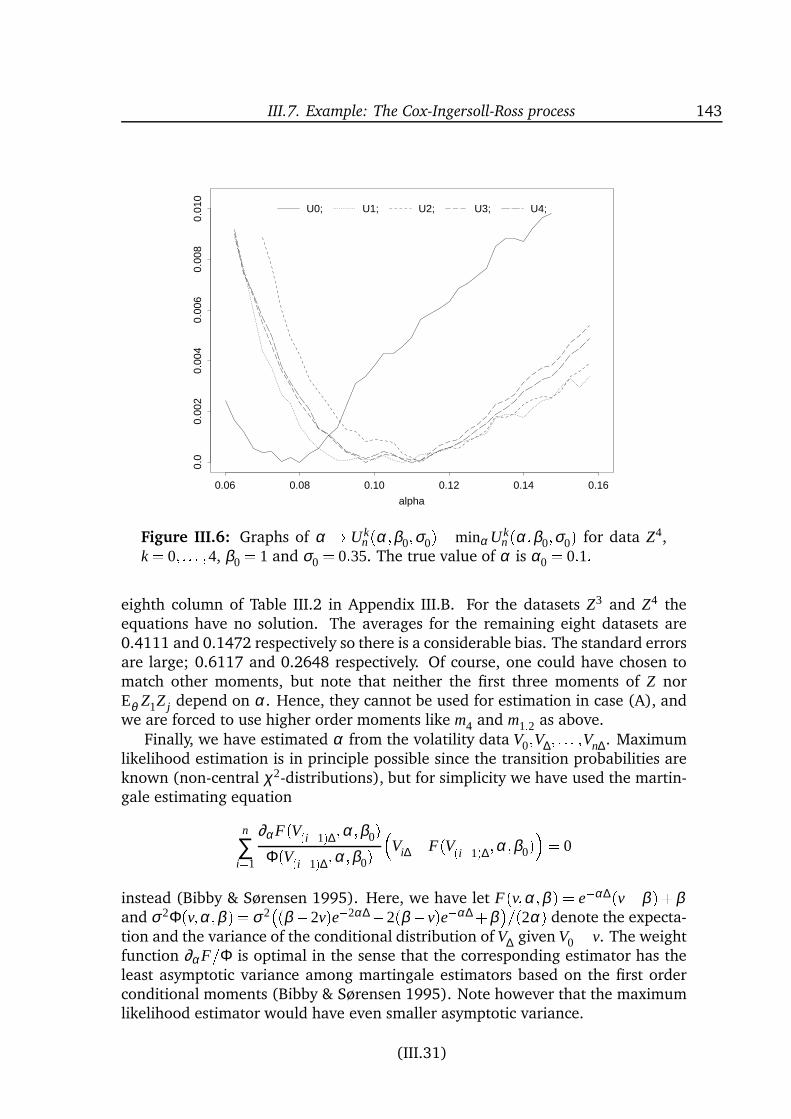
III.7. Example: The Cox-Ingersoll-Ross process 143
alpha
0.06 0.08 0.10 0.12 0.14 0.16
0.0
0.00
20.
004
0.00
60.
008
0.01
0U0; U1; U2; U3; U4;
Figure III.6: Graphs of α ! U kn (α;β0;σ0)minα U k
n (α;β0;σ0) for data Z4,k = 0; : : : ;4, β0 = 1 and σ0 = 0:35. The true value of α is α0 = 0:1:
eighth column of Table III.2 in Appendix III.B. For the datasets Z3 and Z4 theequations have no solution. The averages for the remaining eight datasets are0.4111 and 0.1472 respectively so there is a considerable bias. The standard errorsare large; 0.6117 and 0.2648 respectively. Of course, one could have chosen tomatch other moments, but note that neither the first three moments of Z norEθ Z1Z j depend on α. Hence, they cannot be used for estimation in case (A), andwe are forced to use higher order moments like m4 and m1;2 as above.
Finally, we have estimated α from the volatility data V0;V∆; : : : ;Vn∆. Maximumlikelihood estimation is in principle possible since the transition probabilities areknown (non-central χ2-distributions), but for simplicity we have used the martin-gale estimating equation
n
∑i=1
∂αF(V(i1)∆;α;β0)Φ(V(i1)∆;α;β0) Vi∆F(V(i1)∆;α;β0)= 0
instead (Bibby & Sørensen 1995). Here, we have let F(v;α;β ) = eα∆(vβ )+βand σ2Φ(v;α;β ) = σ2
(β 2v)e2α∆2(β v)eα∆+β=(2α) denote the expecta-
tion and the variance of the conditional distribution of V∆ given V0 = v. The weightfunction ∂αF=Φ is optimal in the sense that the corresponding estimator has theleast asymptotic variance among martingale estimators based on the first orderconditional moments (Bibby & Sørensen 1995). Note however that the maximumlikelihood estimator would have even smaller asymptotic variance.
(III.31)
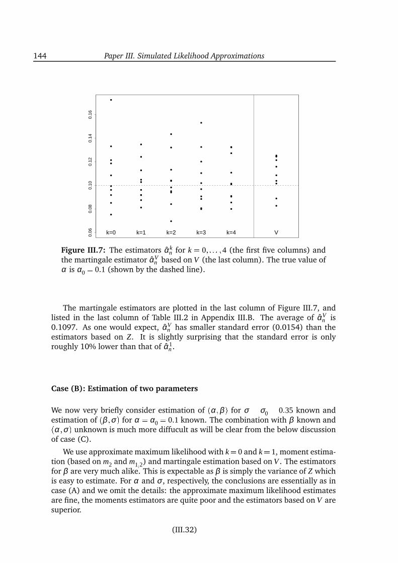
144 Paper III. Simulated Likelihood Approximations
0.06
0.08
0.10
0.12
0.14
0.16
k=0 k=1 k=2 k=3 k=4 V
Figure III.7: The estimators αkn for k = 0; : : : ;4 (the first five columns) and
the martingale estimator αVn based on V (the last column). The true value of
α is α0 = 0:1 (shown by the dashed line).
The martingale estimators are plotted in the last column of Figure III.7, andlisted in the last column of Table III.2 in Appendix III.B. The average of αV
n is0.1097. As one would expect, αV
n has smaller standard error (0.0154) than theestimators based on Z. It is slightly surprising that the standard error is onlyroughly 10% lower than that of α1
n .
Case (B): Estimation of two parameters
We now very briefly consider estimation of (α;β ) for σ = σ0 = 0:35 known andestimation of (β ;σ) for α = α0 = 0:1 known. The combination with β known and(α;σ) unknown is much more diffucult as will be clear from the below discussionof case (C).
We use approximate maximum likelihood with k = 0 and k = 1, moment estima-tion (based on m2 and m1;2) and martingale estimation based on V . The estimatorsfor β are very much alike. This is expectable as β is simply the variance of Z whichis easy to estimate. For α and σ , respectively, the conclusions are essentially as incase (A) and we omit the details: the approximate maximum likelihood estimatesare fine, the moments estimators are quite poor and the estimators based on V aresuperior.
(III.32)
III.7. Example: The Cox-Ingersoll-Ross process 145
Case (C): Estimation of all three parameters
Estimation of one or two parameters was succesful even for k = 0 and k = 1 (aslong as β was one of the unknown parameters). The estimation problem is farmore delicate when all three parameters are unknown, and a larger k is necessaryin order to obtain reasonable estimates.
At first glance it seems promising to use k = 1 for estimation of all three param-eters as well: by the moment considerations in Proposition III.11 it follows thatthe three-dimensional parameter is uniquely determined by the distribution of thepair (Z1;Z2) — and thereby presumably also by the conditional distribution of Z2given Z1. Hence, U1
n should be able to distinguish between different parametervalues.
In practice it turns out that U1n is almost constant — and very close to its min-
imum — on a curve in R3. In other words: U1n has difficulties distinguishing be-
tween parameters on this curve. This is perhaps not too surprising, though. Onecould suspect that only the marginal (invariant) distribution of V is easily deter-mined. The invariant distribution of V is determined completely by two parameterfunctions, namely the shape parameter 2αβ=σ2 and the scale parameter σ2=(2α).One could thus imagine these parameter functions — but not the parameters α, βand σ themselves — to be easy to estimate.
It is easy to get an estimate of the product β of the shape and the scale param-eter; simply use the empirical second moment (or the empirical variance) dividedby ∆,
βn = m2=∆ = 1∆
n
∑i=1
Z2i : (III.26)
But for given β the distribution of (Z1;Z2) wrt. P(α 0;β ;σ 0) and P(α 00;β ;σ 00) can be very
much alike, though not the same, for (α 0;σ 0) and (α 00;σ 00) far from each other —as long as (σ 0)2=(2α 0) is close to (σ 00)2=(2α 00).
This is illustrated by Figure III.8 where we consider level curves for the momentfunctions (α;σ2)!m4(α;β0;σ) = E(α;β0;σ)Z4
1(α;σ2)! m1; j(α;β0;σ) = E(α;β0;σ)Z21Z2
j ; j = 2;3;4;5;
β0 = 1 being the true value of the parameter β . The two solid curves are levelcurves, one for m4 and one for m1;2. Both go through the true value (α0;σ0) =(0:1;0:35), that is, all parameters on the curve for m1, say, have same value ofm1 as the true parameter values. The two level curves are very close, suggestingthat m4(α;β0;σ) is “close” to m4(α0;β0;σ0) if and only if m1;2(α;β0;σ) is “close”
to m1;2(α0;β0;σ0). Although the distribution of (Z1;Z2) is not determined by thesetwo moments alone, the figure indicates that is hard to distinguish between dif-ferent parameter values around the two curves. The three dashed curves in Fig-ure III.8 are level curves for the moments (α;σ2)! m1; j(α;β0;σ) for j = 3;4;5;
they indicate that identification might be easier for larger value of k.
(III.33)
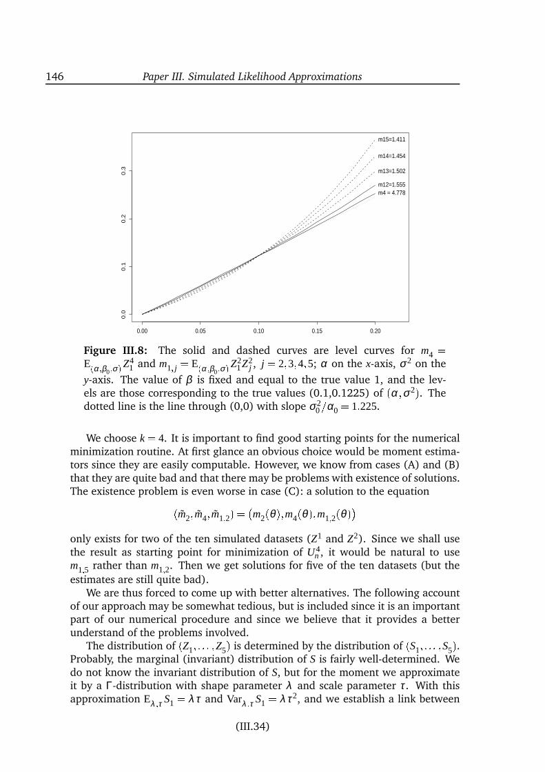
146 Paper III. Simulated Likelihood Approximations
0.00 0.05 0.10 0.15 0.20
0.0
0.1
0.2
0.3
m4 = 4.778m12=1.555
m13=1.502
m14=1.454
m15=1.411
Figure III.8: The solid and dashed curves are level curves for m4 =E(α;β0;σ)Z4
1 and m1; j = E(α;β0;σ)Z21Z2
j , j = 2;3;4;5; α on the x-axis, σ2 on the
y-axis. The value of β is fixed and equal to the true value 1, and the lev-els are those corresponding to the true values (0.1,0.1225) of (α;σ2). Thedotted line is the line through (0,0) with slope σ2
0=α0 = 1:225.
We choose k = 4. It is important to find good starting points for the numericalminimization routine. At first glance an obvious choice would be moment estima-tors since they are easily computable. However, we know from cases (A) and (B)that they are quite bad and that there may be problems with existence of solutions.The existence problem is even worse in case (C): a solution to the equation(m2; m4; m1;2) = m2(θ);m4(θ);m1;2(θ)only exists for two of the ten simulated datasets (Z1 and Z2). Since we shall usethe result as starting point for minimization of U4
n , it would be natural to usem1;5 rather than m1;2. Then we get solutions for five of the ten datasets (but the
estimates are still quite bad).We are thus forced to come up with better alternatives. The following account
of our approach may be somewhat tedious, but is included since it is an importantpart of our numerical procedure and since we believe that it provides a betterunderstand of the problems involved.
The distribution of (Z1; : : : ;Z5) is determined by the distribution of (S1; : : : ;S5).Probably, the marginal (invariant) distribution of S is fairly well-determined. Wedo not know the invariant distribution of S, but for the moment we approximateit by a Γ-distribution with shape parameter λ and scale parameter τ. With thisapproximation Eλ ;τ S1 = λτ and Varλ ;τ S1 = λτ2, and we establish a link between
(III.34)
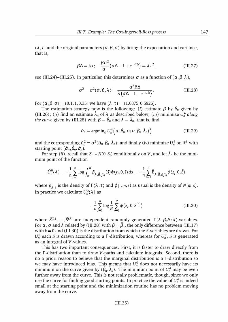
III.7. Example: The Cox-Ingersoll-Ross process 147(λ ;τ) and the original parameters (α;β ;σ) by fitting the expectation and variance,that is,
β∆ = λτ;βσ2
α3
α∆1+ eα∆= λτ2; (III.27)
see (III.24)–(III.25). In particular, this determines σ as a function of (α;β ;λ ),σ2 = σ2(α;β ;λ ) = α3β∆
λα∆1+ eα∆
: (III.28)
For (α;β ;σ) = (0:1;1;0:35) we have (λ ;τ) = (1:6875;0:5926).The estimation strategy now is the following: (i) estimate β by βn given by
(III.26); (ii) find an estimate λn of λ as described below; (iii) minimize U4n along
the curve given by (III.28) with β = βn and λ = λn, that is, find
αn = argminα U4n
α; βn;σ(α; βn; λn) (III.29)
and the corresponding σ2n = σ2(αn; βn; λn); and finally (iv) minimize U4
n on R3 withstarting point (αn; βn; σn).
For step (ii), recall that Zi N(0;Si) conditionally on V , and let λn be the mini-mum point of the function
U0n (λ ) =1
n
n
∑i=1
logZ ∞
0p
λ ;βn=λ(s)ϕ(zi;0; s)ds =1
n
n
∑i=1
Eλ ;βn∆=λ
ϕ(zi;0; S)where pλ ;τ is the density of Γ(λ ;τ) and ϕ(;m;s) as usual is the density of N(m;s).In practice we calculate U0
n (λ ) as1n
n
∑i=1
log1R
R
∑r=1
ϕzi;0; S(r) (III.30)
where S(1); : : : ; S(R) are independent randomly generated Γ(λ ; βn∆=λ )-variables.For α, σ and λ related by (III.28) with β = βn, the only difference between (III.17)with k = 0 and (III.30) is the distribution from which the S-variables are drawn. ForU0
n each S is drawn according to a Γ-distribution, whereas for U0n , S is generated
as an integral of V -values.This has two important consequences. First, it is faster to draw directly from
the Γ-distribution than to draw V -paths and calculate integrals. Second, there isno a priori reason to believe that the marginal distribution is a Γ-distribution sowe may have introduced bias. This means that U0
n does not necessarily have itsminimum on the curve given by (βn; λn). The minimum point of U4
n may be evenfurther away from the curve. This is not really problematic, though, since we onlyuse the curve for finding good starting points. In practice the value of U4
n is indeedsmall at the starting point and the minimization routine has no problem movingaway from the curve.
(III.35)
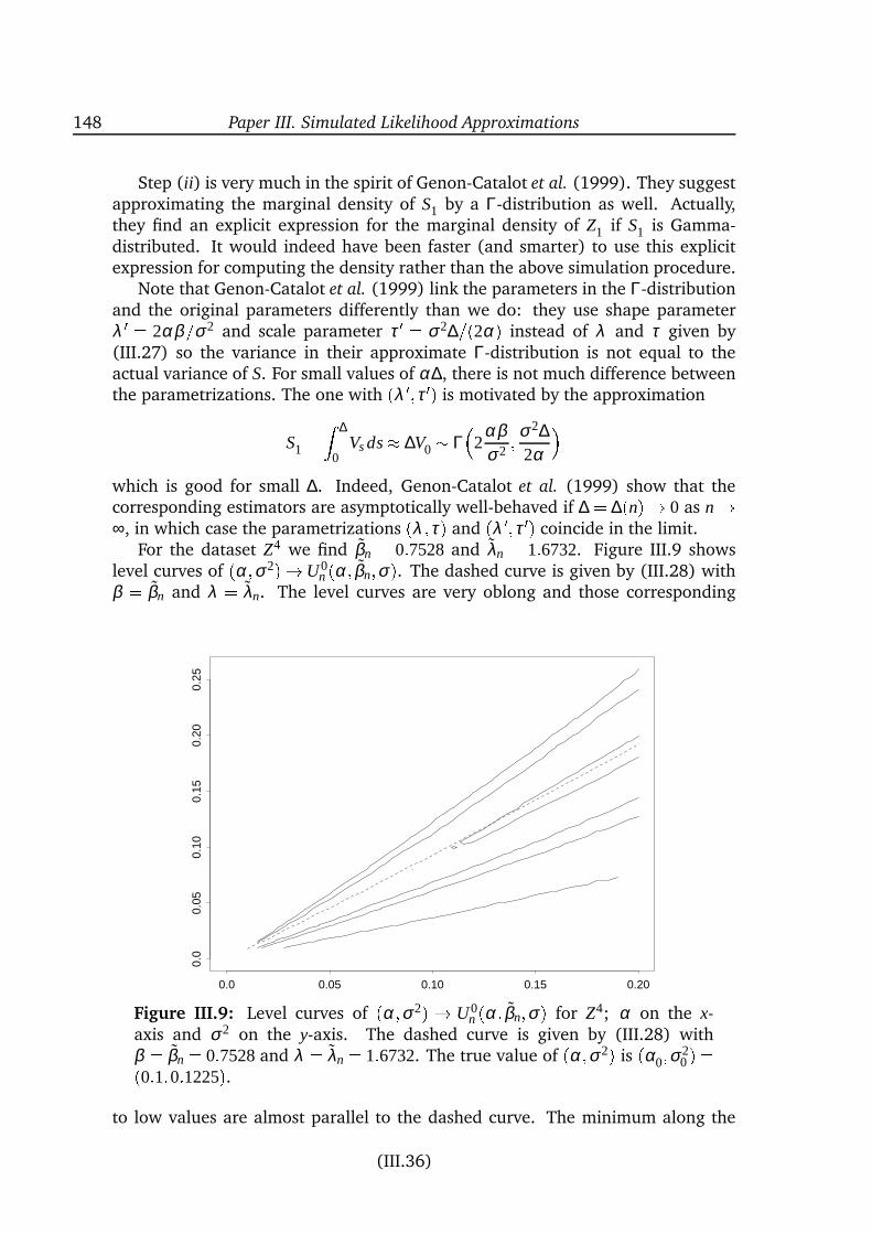
148 Paper III. Simulated Likelihood Approximations
Step (ii) is very much in the spirit of Genon-Catalot et al. (1999). They suggestapproximating the marginal density of S1 by a Γ-distribution as well. Actually,they find an explicit expression for the marginal density of Z1 if S1 is Gamma-distributed. It would indeed have been faster (and smarter) to use this explicitexpression for computing the density rather than the above simulation procedure.
Note that Genon-Catalot et al. (1999) link the parameters in the Γ-distributionand the original parameters differently than we do: they use shape parameterλ 0 = 2αβ=σ2 and scale parameter τ 0 = σ2∆=(2α) instead of λ and τ given by(III.27) so the variance in their approximate Γ-distribution is not equal to theactual variance of S. For small values of α∆, there is not much difference betweenthe parametrizations. The one with (λ 0;τ 0) is motivated by the approximation
S1 = Z ∆
0Vs ds ∆V0 Γ
2
αβσ2 ; σ2∆
2α
which is good for small ∆. Indeed, Genon-Catalot et al. (1999) show that thecorresponding estimators are asymptotically well-behaved if ∆ = ∆(n)! 0 as n !∞, in which case the parametrizations (λ ;τ) and (λ 0;τ 0) coincide in the limit.
For the dataset Z4 we find βn = 0:7528 and λn = 1:6732. Figure III.9 showslevel curves of (α;σ2)!U0
n (α; βn;σ). The dashed curve is given by (III.28) withβ = βn and λ = λn. The level curves are very oblong and those corresponding
0.0 0.05 0.10 0.15 0.20
0.0
0.05
0.10
0.15
0.20
0.25
Figure III.9: Level curves of (α;σ2) ! U0n (α; βn;σ) for Z4; α on the x-
axis and σ2 on the y-axis. The dashed curve is given by (III.28) withβ = βn = 0:7528and λ = λn = 1:6732. The true value of (α;σ2) is (α0;σ2
0) =(0:1;0:1225).to low values are almost parallel to the dashed curve. The minimum along the
(III.36)
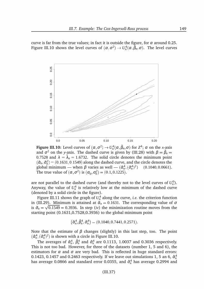
III.7. Example: The Cox-Ingersoll-Ross process 149
curve is far from the true values; in fact it is outside the figure, for α around 0.25.Figure III.10 shows the level curves of (α;σ2)! U4
n (α; βn;σ). The level curves
0.0 0.05 0.10 0.15 0.20
0.0
0.05
0.10
0.15
0.20
0.25
Figure III.10: Level curves of (α;σ2)!U4n (α; βn;σ) for Z4; α on the x-axis
and σ2 on the y-axis. The dashed curve is given by (III.28) with β = βn =0:7528 and λ = λn = 1:6732. The solid circle denotes the minimum point(αn; σ2
n ) = (0:1631;0:1549) along the dashed curve, and the circle denotes theglobal minimum — when β varies as well — (α4
n ;(σ4n )2) = (0:1040;0:0661).
The true value of (α;σ2) is (α0;σ20) = (0:1;0:1225).
are not parallel to the dashed curve (and thereby not to the level curves of U0n ).
Anyway, the value of U4n is relatively low at the minimum of the dashed curve
(denoted by a solid circle in the figure).Figure III.11 shows the graph of U4
n along the curve, i.e. the criterion functionin (III.29). Minimum is attained at αn = 0:1631. The corresponding value of σis σn = p
0:1549= 0:3936. In step (iv) the minimization routine moves from thestarting point (0.1631,0.7528,0.3936) to the global minimum point
α4n ; β 4
n ; σ4n
= (0:1040;0:7441;0:2571):Note that the estimate of β changes (slightly) in this last step, too. The point(α4
n ;(σ4n )2) is shown with a circle in Figure III.10.
The averages of α4n , β 4
n and σ4n are 0.1113, 1.0037 and 0.3036 respectively.
This is not too bad. However, for three of the datasets (number 1, 5 and 6), theestimators for α and σ are very bad. This is reflected in huge standard errors:0.1423, 0.1457 and 0.2463 respectively. If we leave out simulations 1, 5 an 6, α4
nhas average 0.0866 and standard error 0.0355, and σ4
n has average 0.2994 and
(III.37)
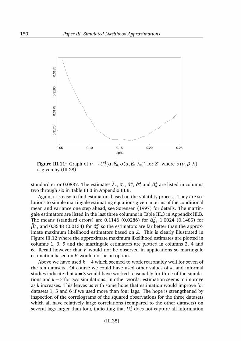
150 Paper III. Simulated Likelihood Approximations
alpha
0.05 0.10 0.15 0.20 0.25
0.31
700.
3175
0.31
800.
3185
Figure III.11: Graph of α !U4n (α; βn;σ(α; βn; λn)) for Z4 where σ(α;β ;λ )
is given by (III.28).
standard error 0.0887. The estimates λn, αn, α4n , σ4
n and σ4n are listed in columns
two through six in Table III.3 in Appendix III.B.
Again, it is easy to find estimators based on the volatility process. They are so-lutions to simple martingale estimating equations given in terms of the conditionalmean and variance one step ahead, see Sørensen (1997) for details. The martin-gale estimators are listed in the last three columns in Table III.3 in Appendix III.B.The means (standard errors) are 0.1146 (0.0286) for αV
n , 1.0024 (0.1485) for
βVn , and 0.3548 (0.0134) for σV
n so the estimators are far better than the approx-imate maximum likelihood estimators based on Z. This is clearly illustrated inFigure III.12 where the approximate maximum likelihood estimates are plotted incolumns 1, 3, 5 and the martingale estimators are plotted in columns 2, 4 and6. Recall however that V would not be observed in applications so martingaleestimation based on V would not be an option.
Above we have used k = 4 which seemed to work reasonably well for seven ofthe ten datasets. Of course we could have used other values of k, and informalstudies indicate that k = 3 would have worked reasonably for three of the simula-tions and k = 2 for two simulations. In other words: estimation seems to improveas k increases. This leaves us with some hope that estimation would improve fordatasets 1, 5 and 6 if we used more than four lags. The hope is strengthened byinspection of the correlograms of the squared observations for the three datasetswhich all have relatively large correlations (compared to the other datasets) onseveral lags larger than four, indicating that U4
n does not capture all information
(III.38)
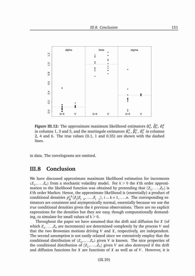
III.8. Conclusion 151
0.0
0.2
0.4
0.6
0.8
1.0
1.2
k=4 V
alpha
k=4 V
beta
k=4 V
sigma
Figure III.12: The approximate maximum likelihood estimators α4n , β 4
n , σ4n
in columns 1, 3 and 5, and the martingale estimators αVn , βV
n , σVn in columns
2, 4 and 6. The true values (0.1, 1 and 0.35) are shown with the dashedlines.
in data. The correlograms are omitted.
III.8 Conclusion
We have discussed approximate maximum likelihood estimation for increments(Z1; : : : ;Zn) from a stochastic volatility model. For k 0 the k’th order approxi-mation to the likelihood function was obtained by pretending that (Z1; : : : ;Zn) isk’th order Markov. Hence, the approximate likelihood is (essentially) a product ofconditional densities pc;k
θ (ZijZik; : : : ;Zi1), i = k+1; : : : ;n. The corresponding es-
timators are consistent and asymptotically normal, essentially because we use thetrue conditional densities given the k previous observations. There are no explicitexpressions for the densities but they are easy, though computationally demand-ing, to simulate for small values of k 0.
Throughout the paper we have assumed that the drift and diffusion for X (ofwhich Z1; : : : ;Zn are increments) are determined completely by the process V andthat the two Brownian motions driving V and X , respectively, are independent.The second assumption is not easily relaxed since we extensively employ that theconditional distribution of (Z1; : : : ;Zn) given V is known. The nice properties ofthe conditional distribution of (Z1; : : : ;Zn) given V are also destroyed if the driftand diffusion functions for X are functions of X as well as of V . However, it is
(III.39)
152 Paper III. Simulated Likelihood Approximations
straightforward to generalize the method so it applies to models where the driftfunction for X is parameter dependent.
Also, the estimation procedure is applicable for other data types with similarproperties, in particular for (other) hidden Markov models. In this respect, theimportant features of the models are the following: (i) given the values of anunobservable process, the observations Z1; : : : ;Zn are independent with a knowndistribution (up to some parameter) determined by the latent process; (ii) theunobserved process is easy to simulate for all values of the parameter. Theseproperties make it easy to simulate values of the approximate likelihood function.
The idea of considering approximations to the likelihood function in terms ofk-lag conditional densities is of course applicable in all kinds of models with com-plicated dependence structures. There are other possible approximations. Forexample, one could split data into tuples of some length, and pretend that thetuples were independent (see Appendix III.A.1). Or one could both conditionforwards and backwards in time, i.e. base estimation on the conditional densi-ties pc;k
θ (ZijZik; : : : ;Zi1;Zi+1; : : : ;Zi+k) given the k previous and the k subsequent
observations. We would get asymptotically well-behaved estimators by these ap-proximations as well. However, since time runs forward, we feel that the approxi-mations based on conditioning backwards in time only, are the most natural.
Finally some comments on possible future work. First, in order for the methodto be really useful one should be able to estimate the variance of the estimator. Theexpression for the asymptotic variance from Theorem III.9 is not useful in practiceas it is given in terms of the unknown k-lag conditional density and its derivatives.Second, there are possibilities of model control built into the method: For each kan estimator of the same parameter is obtained. Consequently, significantly dif-ferent estimators are indications of misspecification of the model. Third, whenproving asymptotic properties for θ k
n , it was implicitly assumed that the approxi-mate likelihood function could be computed accurately. It would be interesting tosee how computation of Lk
n via simulation influence the estimators. Similar workwas done for martingale estimating functions (Kessler & Paredes 1999).
III.A Appendix: Miscellaneous
In this appendix we first give an interpretation of the first term of the k’th order ap-proximation of the log-likelihood function. Next, we state and prove and ergodictheorem and a central limit theorem for the sequence Z.
III.A.1 Split data log-likelihoods
Consider the expression (III.12) for the k’th order approximation to (minus) thelog-likelihood function. We show that the first term may be interpreted as a sumof “split data log-likelihoods” in the sense of Rydén (1994). Assume for simplicitythat the number of observations, n, is a multiple of k+1, that is, J = n=(k+1) is
(III.40)
III.A. Appendix: Miscellaneous 153
an integer, and split (Z1; : : : ;Zn) into J tuples of length k+1,Z1; : : :Zk+1
; : : : ;Znk; : : : ;Zn: (III.31)
If the J tuples were independent, then minus the log-likelihood would be
J
∑j=1
uk+1θ
z( j1)(k+1)+1; : : : ;z j(k+1): (III.32)
It would be just as natural to split the data into one of the sets of J1 (k+1)-tuplesZa+1; : : :Zk+a+1
; : : : ;Z(J2)(k+1)+a+1; : : : ;Zn+a(k+1) (III.33)
for a = 1; : : : ;k although it for each a would leave us with some observations(Z1; : : : ;Za and Zn+ak; : : : ;Zn) not included in a tuple.
Note that (III.33) with a = 0 equals (III.31). For each a = 0; : : : ;k, we get anexpression similar to (III.32) — plus extra terms originating from observations notin a tuple for a 6= 0 — if we pretend that the tuples (III.33) are independent. Thesum over a of minus the log-likelihoods (without the extra terms) is
n1
∑i=k
uk+1θ (zi+1
ik+1); (III.34)
compare with (III.12). In other words: the first term in (III.12) can be interpretedas a sum of log-likelihoods, each of which is obtained by pretending that (k+1)-tuples with no overlap are independent. Note that observations zi for i = 1; : : : ;kand znk+1; : : : ;zn appear in less than k+1 of the terms in (III.34); this could becorrected by including the extra terms mentioned above.
III.A.2 Limit Theorems
We now state and prove an ergodic theorem and a central limit theorem for thesequence Z. The proofs are very similar to the proofs of Theorem 2.2 and Corollary2.1 in Genon-Catalot et al. (1998b).
In the proof of the central limit theorem we use the following result whichfollows immediately from Hall & Heyde (1980, Corollary A.2, page 278): Let AandB be σ -algebras included in F and let U1 and U2 be random variables whichare A - and B-measurable, respectively. If EjU1jr1 < ∞ and EjU2jr2 < ∞ wherer1;r2 > 1 and 1=r1+1=r2 < 1, then
Cov(U1;U2) 8jjU1jjr1jjU2jjr2
α(A ;B)11=r11=r2: (III.35)
Theorem III.12 Suppose that Assumption III.1 holds and let d 1 be arbitrary but
fixed.
(III.41)
154 Paper III. Simulated Likelihood Approximations
1. (Ergodic theorem) For any function ψ : Rd ! R in L1(Pdθ0) it holds that
1n
nd+1
∑i=1
ψ(Zi; : : : ;Zi+d1)! Pdθ0(ψ) = Eθ0
ψ(Z1; : : : ;Zd)Pθ0
-almost surely and in L1(Pθ0) as n! ∞.
2. (Central limit theorem) Let q 1 and consider functions ψ1; : : : ;ψq : Rd ! Rfrom L1(Pd
θ0) with Pd
θ0(ψ j) = Eθ0
ψ j(Z1; : : : ;Zd) = 0 for all j = 1; : : : ;q. Suppose
that there exists an η > 0 such that ψ j is in L2+η(Pdθ0) for all j = 1; : : : ;q and
such that the α-mixing coefficients for Z corresponding to θ0 satisfy the condi-
tion ∑∞m=1αZ(m)η=(2+η) < ∞. Then
Σ jl = Eθ0ψ j(Zd
1)ψl(Zd1)+ ∞
∑m=1
Eθ0
ψ j(Zd1)ψl(Zm+d
m+1)+Eθ0ψl(Zd
1)ψ j(Zm+dm+1)
is well-defined for all j; l = 1; : : : ;q and if the qq matrix Σ = (Σ jl) jl is positive
definite then
1pn
nd+1
∑i=1
ψ1(Zi+d1
i ); : : : ;ψq(Zi+d1i )T ! N(0;Σ)
in distribution wrt. Pθ0as n! ∞.
Proof Under Assumption III.1, Z is α-mixing (Proposition III.2). It is well-knownthat α-mixing implies ergodicity, see e.g. Doukhan (1994, page 21).
For the central limit theorem, first assume that q = 1 and define Yi = ψ(Zi+d1i ),
i 1. Then the σ -algebras generated by Y satisfy
σfYigil
= σfψ(Zi+d1
i )gil
σfZigil+d1
σfYigil+m
= σfψ(Zi+d1
i )gil+m
σfZigil+m
for all s; t 2 N . Hence, the α-mixing coefficients for Y = (Y1;Y2; : : :) satisfy αY (m)αZ(md +1) for m d and thus
∞
∑m=1
αY (m)η=(2+η) d1
∑m=1
αY (m)η=(2+η)+ ∞
∑m=1
αZ(m)η=(2+η) < ∞:It now follows from Hall & Heyde (1980, Corollary 5.1, page 132) that Σ (whichis a real number since q = 1) is non-negative and finite and
Varθ0
n1=2
nd+1
∑i=1
ψ(Zi)! Σ (III.36)
(III.42)
III.B. Appendix: Results from the simulation study 155
as n! ∞. If Σ > 0 then furthermore
n1=2nd+1
∑i=1
ψ1(Zi+d1i ) = n1=2
nd+1
∑i=1
Yi ! N(0;Σ)in distribution.
It might be useful to see how Σ < ∞ and the convergence in (III.36) are ob-tained: the left hand side of (III.36) is equal to
1n
nd+1
∑i; j=1
Eθ0ψ(Zi+d1
i )ψ(Z j+d1j )= Eθ0
ψ2(Zd1)+ 1
n
nd
∑m=1
(nm)Eθ0
ψ(Zd
1)ψ(Zm+dm+1)+ψ(Zm+d
m+1)ψ(Zd1)= Eθ0
ψ2(Zd1)+ nd
∑m=1
Eθ0
ψ(Zd1)ψ(Zm+d
m+1)+Eθ0ψ(Zm+d
m+1)ψ(Zd1) (III.37) 1
n
nd
∑m=1
m
Eθ0ψ(Zd
1)ψ(Zm+dm+1)+Eθ0
ψ(Zm+dm+1)ψ(Zd
1) : (III.38)
Let r1 = r2 = 2+η. It follows by (III.35) that the expectations jEθ0ψ(Zd
1)ψ(Zm+dm+1)j
and jEθ0ψ(Zm+d
m+1)ψ(Zd1)j are bounded by 8jjψ(Zd
1)jj22+η αZ(m)η=(2+η). Hence, by
assumption, Σ is finite and (III.37) converges to Σ. It finally follows by KroneckerLemma that the sum (III.38) converges to zero as n! ∞ so that the convergence(III.36) holds.
Now let q 2. Calculations similar to those above show that Σ jl is well-defined
and can be obtained as a limit of covariances,
Covθ0
n1=2
nd+1
∑i=1
ψ j(Zi);n1=2nd+1
∑i=1
ψl(Zi)! Σ jl
for all j; l = 1: : : ;q. By Cramer-Wold’s device it suffices to show that for any y =(y1; : : : ;yq)T 2 Rq the linear combination
n1=2q
∑j=1
y j
nd+1
∑i=1
ψ j(Zi+d1i ) = n1=2
nd+1
∑i=1
q
∑j=1
y jψ j(Zi+d1i )
converges in distribution to the normal distribution with mean 0 and varianceyT Σy. This follows immediately from the one-dimensional result. III.B Appendix: Results from the simulation study
In this appendix we have collected tables with estimation results from the simu-lation study for the Cox-Ingersoll-Ross process (Section III.7.2). Table III.1 listsempirical moments for the simulated datasets. Table III.2 lists estimators fromcase (A) where only α is unknown, and Table III.3 lists estimators from case (C)where all three parameters are unknown.
(III.43)
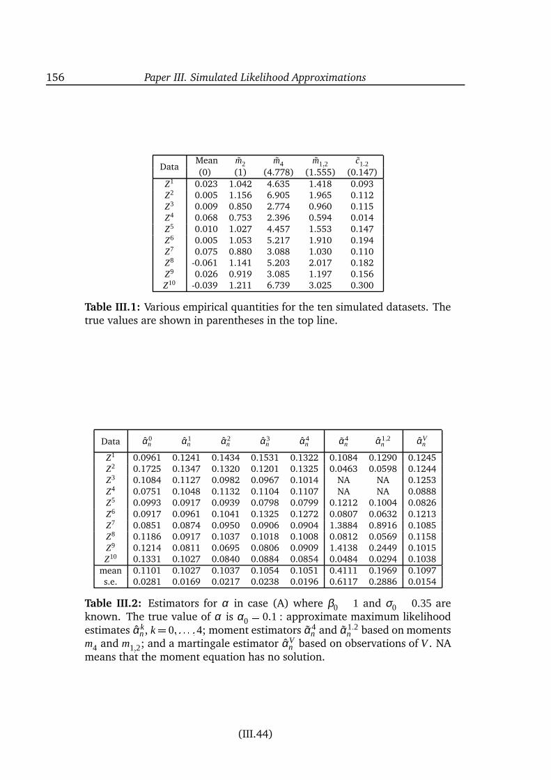
156 Paper III. Simulated Likelihood Approximations
DataMean m2 m4 m1;2 c1;2(0) (1) (4.778) (1.555) (0.147)
Z1 0.023 1.042 4.635 1.418 0.093Z2 0.005 1.156 6.905 1.965 0.112Z3 0.009 0.850 2.774 0.960 0.115Z4 0.068 0.753 2.396 0.594 0.014Z5 0.010 1.027 4.457 1.553 0.147Z6 0.005 1.053 5.217 1.910 0.194Z7 0.075 0.880 3.088 1.030 0.110Z8 -0.061 1.141 5.203 2.017 0.182Z9 0.026 0.919 3.085 1.197 0.156Z10 -0.039 1.211 6.739 3.025 0.300
Table III.1: Various empirical quantities for the ten simulated datasets. Thetrue values are shown in parentheses in the top line.
Data α0n α1
n α2n α3
n α4n α4
n α1;2n αV
n
Z1 0.0961 0.1241 0.1434 0.1531 0.1322 0.1084 0.1290 0.1245Z2 0.1725 0.1347 0.1320 0.1201 0.1325 0.0463 0.0598 0.1244Z3 0.1084 0.1127 0.0982 0.0967 0.1014 NA NA 0.1253Z4 0.0751 0.1048 0.1132 0.1104 0.1107 NA NA 0.0888Z5 0.0993 0.0917 0.0939 0.0798 0.0799 0.1212 0.1004 0.0826Z6 0.0917 0.0961 0.1041 0.1325 0.1272 0.0807 0.0632 0.1213Z7 0.0851 0.0874 0.0950 0.0906 0.0904 1.3884 0.8916 0.1085Z8 0.1186 0.0917 0.1037 0.1018 0.1008 0.0812 0.0569 0.1158Z9 0.1214 0.0811 0.0695 0.0806 0.0909 1.4138 0.2449 0.1015Z10 0.1331 0.1027 0.0840 0.0884 0.0854 0.0484 0.0294 0.1038
mean 0.1101 0.1027 0.1037 0.1054 0.1051 0.4111 0.1969 0.1097s.e. 0.0281 0.0169 0.0217 0.0238 0.0196 0.6117 0.2886 0.0154
Table III.2: Estimators for α in case (A) where β0 = 1 and σ0 = 0:35 areknown. The true value of α is α0 = 0:1 : approximate maximum likelihoodestimates αk
n , k = 0; : : : ;4; moment estimators α4n and α1;2
n based on momentsm4 and m1;2; and a martingale estimator αV
n based on observations of V . NAmeans that the moment equation has no solution.
(III.44)
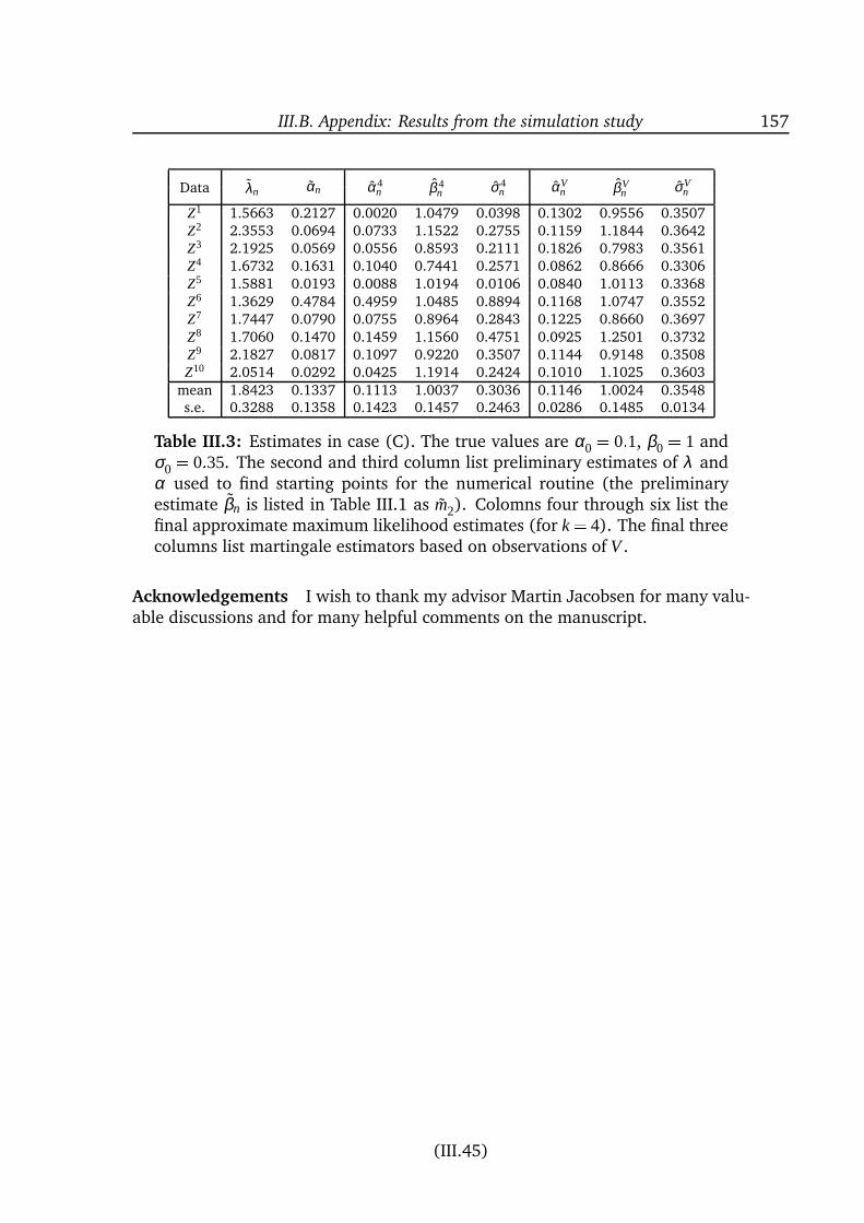
III.B. Appendix: Results from the simulation study 157
Data λn αn α4n β 4
n σ4n αV
n βVn σV
n
Z1 1.5663 0.2127 0.0020 1.0479 0.0398 0.1302 0.9556 0.3507Z2 2.3553 0.0694 0.0733 1.1522 0.2755 0.1159 1.1844 0.3642Z3 2.1925 0.0569 0.0556 0.8593 0.2111 0.1826 0.7983 0.3561Z4 1.6732 0.1631 0.1040 0.7441 0.2571 0.0862 0.8666 0.3306Z5 1.5881 0.0193 0.0088 1.0194 0.0106 0.0840 1.0113 0.3368Z6 1.3629 0.4784 0.4959 1.0485 0.8894 0.1168 1.0747 0.3552Z7 1.7447 0.0790 0.0755 0.8964 0.2843 0.1225 0.8660 0.3697Z8 1.7060 0.1470 0.1459 1.1560 0.4751 0.0925 1.2501 0.3732Z9 2.1827 0.0817 0.1097 0.9220 0.3507 0.1144 0.9148 0.3508Z10 2.0514 0.0292 0.0425 1.1914 0.2424 0.1010 1.1025 0.3603
mean 1.8423 0.1337 0.1113 1.0037 0.3036 0.1146 1.0024 0.3548s.e. 0.3288 0.1358 0.1423 0.1457 0.2463 0.0286 0.1485 0.0134
Table III.3: Estimates in case (C). The true values are α0 = 0:1, β0 = 1 andσ0 = 0:35. The second and third column list preliminary estimates of λ andα used to find starting points for the numerical routine (the preliminaryestimate βn is listed in Table III.1 as m2). Colomns four through six list thefinal approximate maximum likelihood estimates (for k = 4). The final threecolumns list martingale estimators based on observations of V .
Acknowledgements I wish to thank my advisor Martin Jacobsen for many valu-able discussions and for many helpful comments on the manuscript.
(III.45)

Bibliography
Aït-Sahalia, Y. (1996), ‘Nonparametric pricing of interest rate derivative securities’,Econometrica 64, 527–560.
Aït-Sahalia, Y. (1998), Maximum likelihood estimation of discretely sampled diffu-sions: a closed-form approach, Revised version of Working Paper 467, Grad-uate School of Business, University of Chicago.
Andersen, T. G. & Lund, J. (1997), ‘Estimating continuous-time stochastic volatilitymodels of the short-term interest rate’, Journal of Econometrics 77, 343–377.
Andersen, T. G. & Sørensen, B. E. (1996), ‘GMM estimation of a stochastic volatil-ity model: A Monte Carlo study’, Journal of Business and Economic Statistics
14, 328–352.
Arcones, M. A. & Yu, B. (1994), ‘Central limit theorems for empirical and U -processes of stationary mixing sequences’, Journal of Theoretical Probability
7, 47–71.
Banon, G. (1978), ‘Nonparametric identification for diffusion processes’, Siam J.
Control and Optimization 16, 380–395.
Barndorff-Nielsen, O. E., Jensen, J. L. & Sørensen, M. (1998), ‘Some stationaryprocesses in discrete and continuous time’, Advances in Applied Probability
30, 989–1007.
Barndorff-Nielsen, O. E. & Shephard, N. (1999), Non-Gaussian OU based modelsand some of their uses in financial economics, Working Paper 37, Centre forAnalytical Finance, University of Aarhus.
Bera, A. K. & Higgins, M. L. (1993), ‘ARCH models: properties, estimation andtesting’, Journal of Economic Surveys 7, 305–366.
Bibby, B. M. & Sørensen, M. (1995), ‘Martingale estimation functions for discretelyobserved diffusion processes’, Bernoulli 1, 17–39.
Bibby, B. M. & Sørensen, M. (1996), ‘On estimation for discretely observed diffu-sions: A review’, Theory of Stochastic processes 2, 49–56.
160 Bibliography
Bibby, B. M. & Sørensen, M. (1998), Simplified estimating functions for diffusionmodels with a high-dimensional parameter, Preprint 1998-10, Department ofTheoretical Statistics, University of Copenhagen. To appear in Scandinavian
Journal of Statistics.
Bickel, P. J. & Ritov, Y. (1996), ‘Inference in hidden Markov models I: Local asymp-totic normality in the stationary case’, Bernoulli 2, 199–228.
Bickel, P. J., Ritov, Y. & Rydén, T. (1998), ‘Asymptotic normality of the maximum-likelihood estimator for general hidden Markov models’, Annals of Statistics
26, 1614–1635.
Billingsley, P. (1961), ‘The Lindeberg-Levy Theorem for martingales’, Proceedings
of the American Mathematical Society 12, 788–792.
Billingsley, P. (1968), Convergence of Probability Measures, Wiley.
Black, F. & Scholes, M. (1973), ‘The pricing of options and corporate liabilities’,Journal of Political Economy 81, 637–654.
Bradley, R. C. (1986), Basic properties of strong mixing conditions, in E. Eberlein& M. S. Taqqu, eds, ‘Dependence in Probability and Statistics: A Survey ofRecent Results’, Birkhäuser, Boston, pp. 165–192.
Le Breton, A. (1974), Parameter estimation in a linear stochastic differential equa-tion, in ‘Transactions of the Seventh Prague Conference and of the EuropeanMeeting of Statisticians’, pp. 353–366.
Le Breton, A. (1976), ‘On continuous and discrete sampling for parameter estima-tion in diffusion type processes’, Mathematical Programming Study 5, 124–144.
Chan, K. C., Karolyi, G. A., Longstaff, F. A. & Sanders, A. B. (1992), ‘An empiricalcomparison of alternative models of the short-term interest rate’, Journal of
Finance 47, 1209–1227.
Chesney, M. & Scott, L. (1989), ‘Pricing European currency options: a comparisonof the modified Black-Scholes model and a random variance model’, Journal
of Financial and Quantitative Analysis 24, 267–284.
Dacunha-Castelle, D. & Duflo, M. (1986), Probability and Statistics, Vol. 2,Springer-Verlag, New York.
Dacunha-Castelle, D. & Florens-Zmirou, D. (1986), ‘Estimation of the coefficientsof a diffusion from discrete observations’, Stochastics 19, 263–284.
Danielsson, J. (1994), ‘Stochastic volatility in asset prices: estimation with simu-lated maximum likelihood’, Journal of Econometrics 64, 375–400.
Bibliography 161
Danielsson, J. & Richard, J.-F. (1993), ‘Accelerated Gaussian importance samplerwith application to dynamic latent variable models’, Journal of Applied Econo-
metrics 8, S153–S173.
Doukhan, P. (1994), Mixing: Properties and Examples, Lecture Notes in Statistics85, Springer-Verlag, New York.
Elerian, O., Chib, S. & Shephard, N. (2000), Likelihood inference for discretely ob-served non-linear diffusions, Economics discussion paper 146, Nuffield Col-lege, Oxford. To appear in Econometrica.
Eraker, B. (1998), MCMC analysis of diffusion models with application to finance,Discussion paper 1998-5, Department of Finance and Management Science,Norwegian School of Economics and Business Administration.
Florens-Zmirou, D. (1989), ‘Approximate discrete-time schemes for statistics ofdiffusion processes’, Statistics 20, 547–557.
Florens-Zmirou, D. (1993), ‘On estimating the diffusion coefficient from discreteobservations’, Journal of Applied Probability 30, 790–804.
Gallant, A. R., Hsieh, D. & Tauchen, G. (1997), ‘Estimation of stochastic volatilitymodels with diagnostics’, Journal of Econometrics 81, 159–192.
Gallant, A. R. & Long, J. R. (1997), ‘Estimating stochastic differential equationsefficiently by minimum chi-squared’, Biometrika 84, 125–141.
Gallant, A. R. & Tauchen, G. (1996), ‘Which moments to match?’, Econometric
Theory 12, 657–681.
Genon-Catalot, V., Jeantheau, T. & Laredo, C. (1998a), ‘Limit theorems for dis-cretely observed stochastic volatility models’, Bernoulli 4, 283–303.
Genon-Catalot, V., Jeantheau, T. & Laredo, C. (1998b), Stochastic volatility mod-els as hidden Markov models and statistical applications, Preprint 1998-22,Equipe d’Analyse et de Mathématiques Appliquées, Université de Marne-la-Vallée.
Genon-Catalot, V., Jeantheau, T. & Laredo, C. (1999), ‘Parameter estimation fordiscretely observed stochastic volatility models’, Bernoulli 5, 855–872.
Ghysels, E., Harvey, A. C. & Renault, E. (1996), Stochastic volatility, in G. S. Mad-dala & C. R. Rao, eds, ‘Statistical Methods in Finance’, Vol. 14 of Handbook
of Statistics, North-Holland, Amsterdam, pp. 119–191.
Gourieroux, C., Monfort, A. & Renault, E. (1993), ‘Indirect inference’, Journal of
Applied Econometrics 8, S85–S118.
Hall, P. & Heyde, C. C. (1980), Martingale Limit Theory and its Application, Aca-demic Press, New York.

162 Bibliography
Hansen, L. P. (1982), ‘Large sample properties of generalized method of momentsestimators’, Econometrica 50, 1029–1054.
Hansen, L. P. & Scheinkman, J. A. (1995), ‘Back to the future: generating momentimplications for continuous-time Markov processes’, Econometrica 63, 767–804.
Harvey, A., Ruiz, E. & Shephard, N. (1994), ‘Multivariate stochastic variance mod-els’, Review of Economic Studies 61, 247–264.
Heston, S. L. (1993), ‘A closed-form solution for options with stochastic volatil-ity with applications to bond and currency options’, The Review of Financial
Studies 6, 327–343.
Heyde, C. C. (1997), Quasi-Likelihood and its Application: A General Approach to
Optimal Parameter Estimation, Springer-Verlag, New York.
Honoré, P. (1997), Maximum likelihood estimation of non-linear continuous-time term-structure models, Working paper 1997-7, Department of Finance,Aarhus School of Business.
Hull, J. & White, A. (1987), ‘The pricing of options on assets with stochastic volatil-ities’, The Journal of Finance 42, 281–300.
Hull, J. & White, A. (1988), ‘An analysis of the bias in option pricing caused by astochastic volatility’, Advances in Futures and Options Research 3, 29–61.
Jacobsen, M. (1998), Discretely observed diffusions: classes of estimating func-tions and small ∆-optimality, Preprint 1998-11, Department of TheoreticalStatistics, University of Copenhagen. To appear in Scandinavian Journal of
Statistics.
Jacquier, E., Polson, N. G. & Rossi, P. E. (1994), ‘Bayesian analysis of stochasticvolatility models (with discussion)’, Journal of Business and Economic Statis-
tics 12, 371–417.
Jensen, J. L. & Petersen, N. V. (1999), ‘Asymptotic normality of the maximumlikelihood estimator in state space models’, Annals of Statistics 27, 514–535.
Jiang, G. J. & Knight, J. L. (1997), ‘A nonparametric approach to the estimation ofdiffusion processes, with an application to a short-term interest rate model’,Econometric Theory 13, 615–645.
Karatzas, I. & Shreve, S. E. (1991), Brownian Motion and Stochastic Calculus, 2ndedn, Springer-Verlag, New York.
Karlin, S. & Taylor, H. M. (1981), A Second Course in Stochastic Processes, AcademicPress, New York.
Bibliography 163
Kessler, M. (2000), ‘Simple and explicit estimating functions for a discretely ob-served diffusion process’, Scandinavian Journal of Statistics 27, 65–82.
Kessler, M. & Paredes, S. (1999), Computational aspects related to martingaleestimating functions for a discretely observed diffusion, Manuscript, Depar-tamento de Matemática Aplicada y Estadística, Universidad Politécnica deCartagena.
Kessler, M. & Sørensen, M. (1999), ‘Estimating equations based on eigenfunctionsfor a discretely observed diffusion process’, Bernoulli 5, 299–314.
Kim, S., Shephard, N. & Chib, S. (1998), ‘Stochastic volatility: likelihood inferenceand comparison with ARCH models’, Review of Economic Studies 65, 361–393.
Lipster, R. S. & Shiryayev, A. N. (1977), Statistics of Random Processes, Vol. 1,Springer-Verlag, New York.
Lo, A. W. (1988), ‘Maximum likelihood estimation of generalized Itô processeswith discretely sampled data’, Econometric Theory 4, 231–247.
Nelson, D. B. (1990), ‘ARCH models as diffusion approximations’, Journal of
Econometrics 45, 7–38.
Nelson, D. B. (1992), ‘Filtering and forecasting with misspecified ARCH models I’,Journal of Econometrics 52, 61–90.
Nielsen, J. N., Vestergaard, M. & Madsen, H. (2000), Estimation in continuous-time stochastic volatility models using nonlinear filters. To appear in Inter-
national Journal of Theoretical and Applied Finance.
Overbeck, L. & Rydén, T. (1997), ‘Estimation in the Cox-Ingersoll-Ross model’,Econometric Theory 13, 430–461.
Pedersen, A. R. (1995a), ‘Consistency and asymptotic normality of an approximatemaximum likelihood estimator for discretely observed diffusion processes’,Bernoulli 1(3), 257–279.
Pedersen, A. R. (1995b), ‘A new approach to maximum likelihood estimation forstochastic differential equations based on discrete observations’, Scandina-
vian Journal of Statistics 22, 55–71.
Pollard, D. (1984), Convergence of Stochastic Processes, Springer-Verlag, New York.
Poulsen, R. (1999), Approximate maximum likelihood estimation of discretely ob-served diffusion processes, Working paper 29, Centre for Analytical Finance,Aarhus.
Rogers, L. C. G. & Williams, D. (1987), Diffusions, Markov Processes, and Martin-
gales, Vol. 2: Itô Calculus, Wiley.
164 Bibliography
Rydén, T. (1994), ‘Consistent and asymptotically normal parameter estimates forhidden Markov models’, Annals of Statistics 22, 1884–1895.
Scott, L. O. (1987), ‘Option pricing when the variance changes randomly: theory,estimation and an application’, Journal of Financial and Quantitative analysis
22, 419–438.
Shephard, N. (1996), Statistical aspects of ARCH and stochastic volatility, in D. R.Cox, D. V. Hinkley & O. E. Barndorff-Nielsen, eds, ‘Time Series Models inEconometrics, Finance and Other Fields’, Chapman & Hall, London, pp. 1–67.
Sørensen, H. (1998a), Approximation of the score functions for diffusion pro-cesses, Preprint 1998-8, Department of Theoretical Statistics, University ofCopenhagen.
Sørensen, H. (2000), Estimation of diffusion parameters for discretely observeddiffusion processes, Preprint 2000-1, Department of Theoretical Statistics,University of Copenhagen.
Sørensen, M. (1997), Estimating functions for discretely observed diffusions: Areview, in I. V. Basawa, V. P. Godambe & R. L. Taylor, eds, ‘Selected Proceed-ings of the Symposium on Estimating Functions’, Vol. 32, IMS Lecture notes,pp. 305–325.
Sørensen, M. (1998b), On asymptotics of estimating functions, Preprint 1998-6,Department of Theoretical Statistics, University of Copenhagen. To appearin Brazilian Journal of Probability and Statistics.
Sørensen, M. (1999), Prediction-based estimating functions, Preprint 1999-5, De-partment of Theoretical Statistics, University of Copenhagen.
Stein, E. M. & Stein, J. C. (1991), ‘Stock price distributions with stochastic volatil-ity: an analytic approach’, The Review of Financial Studies 4, 727–752.
van der Vaart, A. W. & Wellner, J. A. (1996), Weak Convergence and Empirical
Processes, Springer-Verlag, New York.
Wiggins, J. B. (1987), ‘Options values under stochastic volatility’, Journal of Fi-
nancial Economics 19, 351–372.