indoor localization of mobile devices based on wi-fi ... · devices based on wi-fi signals using...
TRANSCRIPT
Indoor Localization of MobileDevices Based on Wi-Fi Signals
Using Raytracing SupportedAlgorithms.
Diploma Thesis
Dirk Rothe
RWTH Aachen University, Germany
Chair for Communication and Distributed Systems
Advisors:
Dipl.-Inform. Nicolai ViolProf. Dr.-Ing. Klaus Wehrle
Prof. Dr. Leif Kobbelt
Registration date: 2011-08-22Submission date: 2012-02-22


I hereby affirm that I composed this work independently and used no other than thespecified sources and tools and that I marked all quotes as such.
Hiermit versichere ich, dass ich die Arbeit selbststandig verfasst und keine anderenals die angegebenen Quellen und Hilfsmittel benutzt sowie Zitate kenntlich gemachthabe.
Aachen, den 22. Februar 2012


Abstract
This thesis focuses on the localization problem adapted to the constraints of araytracer simulated signal distribution for Wi-Fi capable mobile devices in indoor
scenarios. The localization problem is defined as predicting the most probablelocations for an observed sequence of Wi-Fi signal strength readings. An accurately
performing solution is of high interest because Wi-Fi signals can be observedcheaply due to an already widespread deployment of Access Points. For an efficientanalysis of the problem, a framework is implemented that combines the raytracing,
the localization and evaluation components. Based on this framework, it isinvestigated whether the raytracing tool provides an effective basis for an accurate
Wi-Fi localization system. Furthermore, the performance of a Hidden MarkovModel, a Particle Filter and a Nearest Neighbour based localization approach areevaluated on automatically trained raytracer models. Therefore, a representativecorpus of location annotated signal measurements is assembled and subsequentlyemployed for a thorough investigation of the algorithm properties with respect to
tracking the device in scenes of various complexity. The trained Wi-Fi signalstrength predictions diverge in average by 4dBm from the real measurements.
Under these predictions, the tracking algorithms reach a localization accuracy ofabout 1.5m on pathways and degrades up to 4m in complex scenes like stairways.


Acknowledgments
I wish to thank my supervisor Nicolai Viol and Prof. Dr. Wehrle for the opportunityto work on the fascinating subject of this thesis. Without their guidance, theirsupport and especially the challenging and constructive discussions, the thesis wouldnot have been completed with a satisfying result.
Beside my supervisor, I want to thank my team at semantics for allowing me todedicate my time fully onto the presented topic. Without their efforts, this thesiswould not have been possible.
I’m also grateful for all the help of my friends: Mirjam, Kadir, Albert, and Chrissito proofread the text and dig out all the invisible inconsistencies.
Last, but not least, I must thank my wife Christine for her support and endlesspatience during the last six months.

Contents
1 Introduction 1
1.1 Radio Propagation . . . . . . . . . . . . . . . . . . . . . . . . . . . . 2
1.2 Localization Algorithms . . . . . . . . . . . . . . . . . . . . . . . . . 3
1.3 Framework and Implementation . . . . . . . . . . . . . . . . . . . . . 4
1.4 Evaluation . . . . . . . . . . . . . . . . . . . . . . . . . . . . . . . . . 5
1.5 Outline . . . . . . . . . . . . . . . . . . . . . . . . . . . . . . . . . . . 6
2 Background 7
2.1 Radio Propagation Model . . . . . . . . . . . . . . . . . . . . . . . . 7
2.1.1 PHOTON Raytracer . . . . . . . . . . . . . . . . . . . . . . . 10
2.1.2 Optimization with Genetic Algorithms . . . . . . . . . . . . . 12
2.1.3 Error . . . . . . . . . . . . . . . . . . . . . . . . . . . . . . . . 13
2.2 Positioning . . . . . . . . . . . . . . . . . . . . . . . . . . . . . . . . 13
2.2.1 Techniques . . . . . . . . . . . . . . . . . . . . . . . . . . . . . 14
2.3 Tracking . . . . . . . . . . . . . . . . . . . . . . . . . . . . . . . . . . 16
2.3.1 Mobility Models . . . . . . . . . . . . . . . . . . . . . . . . . . 16
2.3.2 Error . . . . . . . . . . . . . . . . . . . . . . . . . . . . . . . . 18
2.4 Bayesian Pattern Recognition . . . . . . . . . . . . . . . . . . . . . . 18
2.5 Hidden Markov Models . . . . . . . . . . . . . . . . . . . . . . . . . . 21
2.5.1 Decision Rule . . . . . . . . . . . . . . . . . . . . . . . . . . . 23
2.5.2 Viterbi Algorithm . . . . . . . . . . . . . . . . . . . . . . . . . 23
2.5.3 Higher Order Models . . . . . . . . . . . . . . . . . . . . . . . 25
2.5.4 Logspace . . . . . . . . . . . . . . . . . . . . . . . . . . . . . . 25
2.5.5 Pruning . . . . . . . . . . . . . . . . . . . . . . . . . . . . . . 27
2.5.6 Training . . . . . . . . . . . . . . . . . . . . . . . . . . . . . . 28
2.6 Continuous Models . . . . . . . . . . . . . . . . . . . . . . . . . . . . 28
2.6.1 Linear Dynamic System . . . . . . . . . . . . . . . . . . . . . 28
2.6.2 Particle Filter . . . . . . . . . . . . . . . . . . . . . . . . . . . 29
2.7 Least Mean Squared Error . . . . . . . . . . . . . . . . . . . . . . . . 30
2.8 Summary . . . . . . . . . . . . . . . . . . . . . . . . . . . . . . . . . 31
3 Related Work 33
3.1 Radio Propagation . . . . . . . . . . . . . . . . . . . . . . . . . . . . 33
3.1.1 2D-Raytracer Models . . . . . . . . . . . . . . . . . . . . . . . 34
3.1.2 3D-Raytracer Models . . . . . . . . . . . . . . . . . . . . . . . 35
3.2 Positioning and Tracking . . . . . . . . . . . . . . . . . . . . . . . . . 37
3.2.1 Hidden Markov Models . . . . . . . . . . . . . . . . . . . . . . 37
3.2.2 Particle Filters . . . . . . . . . . . . . . . . . . . . . . . . . . 39
3.2.3 Nearest Neighboor based Approaches . . . . . . . . . . . . . . 41
3.3 Summary . . . . . . . . . . . . . . . . . . . . . . . . . . . . . . . . . 42
4 Design 43
4.1 General Overview . . . . . . . . . . . . . . . . . . . . . . . . . . . . . 43
4.2 Radio Propagation . . . . . . . . . . . . . . . . . . . . . . . . . . . . 44
4.2.1 Model . . . . . . . . . . . . . . . . . . . . . . . . . . . . . . . 45
4.2.2 Parameter Estimation . . . . . . . . . . . . . . . . . . . . . . 45
4.2.2.1 Initialization . . . . . . . . . . . . . . . . . . . . . . 46
4.2.2.2 Optimization . . . . . . . . . . . . . . . . . . . . . . 46
4.2.3 Device Specific Adaptation . . . . . . . . . . . . . . . . . . . . 47
4.3 Positioning and Tracking . . . . . . . . . . . . . . . . . . . . . . . . . 48
4.3.1 Hidden Markov Model . . . . . . . . . . . . . . . . . . . . . . 49
4.3.1.1 Parameter Estimation . . . . . . . . . . . . . . . . . 50
4.3.1.2 Emission Probabilities . . . . . . . . . . . . . . . . . 50
4.3.1.3 Transition Probabilities . . . . . . . . . . . . . . . . 51
4.3.1.4 Pruning . . . . . . . . . . . . . . . . . . . . . . . . . 53
4.3.1.5 Result Sequence . . . . . . . . . . . . . . . . . . . . 55
4.3.2 Particle Filter . . . . . . . . . . . . . . . . . . . . . . . . . . . 55
4.3.2.1 Emission Probabilities . . . . . . . . . . . . . . . . . 55
4.3.2.2 Transition Probabilities . . . . . . . . . . . . . . . . 55
4.3.2.3 Sample Impoverishment . . . . . . . . . . . . . . . . 56
4.3.2.4 Result Sequence . . . . . . . . . . . . . . . . . . . . 57
4.4 Devices . . . . . . . . . . . . . . . . . . . . . . . . . . . . . . . . . . 57
4.5 Fat Client . . . . . . . . . . . . . . . . . . . . . . . . . . . . . . . . . 57
4.6 Evaluation . . . . . . . . . . . . . . . . . . . . . . . . . . . . . . . . . 59
4.7 Summary . . . . . . . . . . . . . . . . . . . . . . . . . . . . . . . . . 60
5 Implementation 63
5.1 Third Party Libraries . . . . . . . . . . . . . . . . . . . . . . . . . . . 64
5.2 Modules . . . . . . . . . . . . . . . . . . . . . . . . . . . . . . . . . . 67
5.2.1 Server . . . . . . . . . . . . . . . . . . . . . . . . . . . . . . . 68
5.2.2 Localization Algorithms . . . . . . . . . . . . . . . . . . . . . 70
5.2.3 Fat Client . . . . . . . . . . . . . . . . . . . . . . . . . . . . . 72
5.3 Summary . . . . . . . . . . . . . . . . . . . . . . . . . . . . . . . . . 73
6 Evaluation 75
6.1 Radio Propagation Model . . . . . . . . . . . . . . . . . . . . . . . . 76
6.1.1 Scene and Setup . . . . . . . . . . . . . . . . . . . . . . . . . 76
6.1.1.1 3D-Model and Materials . . . . . . . . . . . . . . . . 76
6.1.1.2 Accesspoints . . . . . . . . . . . . . . . . . . . . . . 77
6.1.1.3 Devices . . . . . . . . . . . . . . . . . . . . . . . . . 78
6.1.1.4 Training Corpus . . . . . . . . . . . . . . . . . . . . 79
6.1.2 Training of free Parameters . . . . . . . . . . . . . . . . . . . 80
6.1.2.1 Granularity of the 3D geometry . . . . . . . . . . . . 81
6.1.2.2 Multiple Devices . . . . . . . . . . . . . . . . . . . . 82
6.2 Localization . . . . . . . . . . . . . . . . . . . . . . . . . . . . . . . . 82
6.2.1 Scene and Setup . . . . . . . . . . . . . . . . . . . . . . . . . 82
6.2.2 Synthetic Measurements . . . . . . . . . . . . . . . . . . . . . 84
6.2.3 Real World Measurements . . . . . . . . . . . . . . . . . . . . 87
6.2.3.1 Device Adaptation . . . . . . . . . . . . . . . . . . . 88
6.2.3.2 Multiple Devices . . . . . . . . . . . . . . . . . . . . 89
6.2.3.3 Granularity of the 3D geometry . . . . . . . . . . . . 91
6.3 Summary . . . . . . . . . . . . . . . . . . . . . . . . . . . . . . . . . 92
7 Conclusion 95
7.1 Future Work . . . . . . . . . . . . . . . . . . . . . . . . . . . . . . . . 96
Bibliography 99
A Appendix 103
A.1 List of Abbreviations . . . . . . . . . . . . . . . . . . . . . . . . . . . 103
A.2 Localization Paths . . . . . . . . . . . . . . . . . . . . . . . . . . . . 104
A.3 Synthetic Localization Error Tables . . . . . . . . . . . . . . . . . . . 108
A.4 2D Localization Result . . . . . . . . . . . . . . . . . . . . . . . . . . 111
A.5 Optimization Process . . . . . . . . . . . . . . . . . . . . . . . . . . . 111
1Introduction
The problem of determining the location of a person or an object is an ancient one.Many different methods were employed over the recent centuries. For example, thenavigation of ships has been supported by referencing to the celestial map of stars,lighthouses or even by transportable devices known as sextants. More recently,tracking the location of vehicles is primarily done with the support of satellite basedsystems. The first deployed of these systems is the well known GPS system. Fromair planes over ships to cars, nearly every modern vehicle today is able to determineits position with an accuracy down to a few meters. But the need for localizationsolutions is not just confined to vehicles of transportation services. For example,due to the now ubiquitous availability of powerful mobile computing devices, therealization of personalized context- and location-aware applications has become anactive field of research. But the natural habitats of human individuals, the indoorenvironments, are dark zones for the signals of the GPS satellites.
The lack of a comparable efficient indoor localization method motivates the researchactivities into alternative localization systems that are specifically adapted to theseenvironments. Therefore, indoor localization solutions have been based on variousinformation sources that reflect the constraints of the different use-cases. Whereas ahypothesized domestic robot can be specifically designed to carry multiple sensors asoptical cameras, ultra-sound or infra-red devices, this degree of freedom is not givenfor the localization of human beings. There, the sensors need also to be unobtrusivewhich can be ensured by sensing signals of communication networks.
This thesis will focus on the signals of IEEE 802.11 wireless networks as the pri-mary source of information to approach the localization problem. The importantadvantage of Wi-Fi, in contrast to other technologies, is the inexpensive hardwareand the already dense deployment of Wi-Fi Access Points (APs) in urban areas. Forexample, at the RWTH Aachen University it is most likely to be in range of at least 5APs across the campus side 1. Widespread interest into these signal-strength based
1Although it has to be noted, that RWTH is an university with a strong technical background,and thus probably a site with a high saturation of APs. But by interpolating the history it canalso be expected that the density of deployed Wi-Fi infrastructure still increases.
2 1. Introduction
localization solutions has been induced by the RADAR [2] system developed at Mi-crosoft Research at the year 2000. The system uses the received signals strengthsof a number of APs and an analytical model for the impact of an obstacle on thesignal strength to determine the position of a mobile device with respect to a 2Dfloor map. From the structure of the RADAR system can be concluded that theproblem formulation has two major aspects:What is the distribution of the signal strengths and how is this information processedalgorithmically?
1.1 Radio Propagation
The first aspect relates to the nature of the Wi-Fi signals and rises the followingquestions. How are the signals distributed in the localization space? How are theypropagated from the AP source? These questions lead to the concept of radio prop-agation models. These models can be specified at different levels of complexity butthey have in common, that they allow a prediction of the Wi-Fi signal distributionover the targeted areas. This prediction can then be used to drive the decisionprocess that leads to a localization result.
Consequently, the generation of an accurate radio propagation model was the firstfocus of this thesis. The primary source for the investigated propagation model isthe so called PHOTON raytracer [23] that was developed recently by Arne Schmitzat the chair of I8 of the RWTH. The performance of the GPU-driven raytracer,with respect to radio signal propagation, was in the first place examined for urbanoutdoor environments, but it is designed for the general application to arbitraryindoor and outdoor environments. A basic evaluation of the model capabilities foran indoor scenario was conducted in an earlier work by Schmitz [24].
In order to simulate the propagation of the AP emitted radio signals accurately, theraytracer has to be configured with parameters that relate to the physical propertiesof the involved entities. The first entity is the AP that is basically configured tobe an isotropic radio sender with a scalar antenna gain. The other simulation rele-vant entities compose the structure of the building and can basically be understoodas material annotated scene geometry. Thus, the scene geometry is a mandatoryprerequisite for the raytracer and the material parameters have to be determinedindependently.
The target indoor scenario for the evaluation of this thesis is the UMIC office buildingwith four levels and a size of 15m × 60m × 9m. The 3D geometry of the buildingwas modelled by using the software Blender2. 10 different types of materials weredefined and accordingly attached to the mesh model. Further details on the modelproperties and the materials are described more formally in the evaluation chapter6.1.1.
The parameters of the materials, specifically the coefficients controlling the rate ofabsorption and reflection of the given building are assumed to be unknown in order toperform the raytracing simulation. To acquire these parameters, a training techniquebased on evolutionary concepts, more precisely Genetic Algorithms, is devised and
2The open source toolkit Blender is freely available at http://www.blender.org/.
1.2. Localization Algorithms 3
implemented to distribute the computational demanding search for the unknownparameters over an array of GPU-nodes. The procedure has been determined toyield adequate material parameters for the simulation of the signal distribution overthe 2 · 106 voxel3 resolution of the 8100m2 volume for UMIC scene.
1.2 Localization Algorithms
The second topic of the thesis deploys these radio propagation models for the design,implementation and analysis of different localization algorithms. The algorithms ex-ploit the information provided by the propagation models and the available knowl-edge about the nature of the environment. For example, information about thestructure of the building is already available in the form of the scene geometry usedfor the PHOTON raytracer. From this geometry, for example the knowledge aboutunreachable zones in the location space can be derived. The algorithms were chosenby studying the related literature to this topic and by applying prior knowledgeof Bayesian pattern recognition principles to this field of research. The first of thethree analysed algorithms is a nearest neighbour based technique, named Least MeanSquared Error (LMSE), that was also used by the mentioned RADAR system. Thesecond is based on Hidden Markov Models (HMM) and the third one uses a ParticleFilter (PF) based approach.
All three techniques can be inferred from the Bayesian decision theory but only theHMM and the PF are conceptually related. The primary difference between theLMSE and the HMM/PF is rooted in its model assumptions that ignore the sequen-tial nature of the tracking problem. With respect to the scope of this thesis, thetracking problem is defined as follows: Given a sequence of RSSI readings the optimalsequence of locations has to be found. It is reasonable to assume that adjacent RSSIreadings are related due to constraints imposed by the physical world. Or spokenin the terms of probability theory: Temporal adjacent readings are not statisticallyindependent. The HMM and PF based approaches presented in this thesis makeexplicit use of these dependencies, whereas the LMSE does not and thereby retainsa simple structure 4.
The HMM and PF technique exploit the additional information contained in the timedriven sequentiality of the tracking problem. Both model the concept of movementfrom one location to another in successive steps. In terms of probability theory: Theyassume a conditional probability for moving to the location s under the conditionto come from location s′ which should be denoted as p(s|s′) 5. Furthermore, bothmake use of the radio propagation model to relate an RSSI measurement vector to alocation in space. This can be understood as the conditional probability to receivethe RSSI vector x at the location s. This probability is denoted as p(x|s). Andfinally, they combine these two probabilities iteratively for all measurements of theobserved sequence to predict the most probable sequence of positions. So where arethe differences, why care for both?
3A 3D pixel, a discretized volume of space.4The simplicity of the LMSE makes it a valuable tool to evaluate the quality of radio propagation
models with regard to the localization problem.5A location is understood to represent an abstract state from the search space of possible
locations, therefore it is denoted as s instead of l.

4 1. Introduction
In the HMM case, the locations are assumed to be discrete and enumerable. There-fore, the possible combinations of these locations, the probable solutions to thetracking problem, are enumerable, too. Since these are a huge number of possi-ble location sequences, the HMM model has to make assumptions that restrict thesearch space to a tractable size. Only depending on the quality of the assumptionsthe algorithm predicts the most probable location sequence of all possible solutions.
The PF makes use of a continuous location space thus avoiding the error inducedby the coarseness of an eventual discretization of the space. Instead of searching forsolutions by enumerating the search space, the algorithm generates solutions thatare elements of an infinite solution space. Whereas the HMM uses the mentionedconditional probabilities to assign probabilities (or scores) to all candidate sequences,the PF generates a subset of all solutions by simulating the progress of the modelledstochastic process by sampling from the conditionals. Due to this properties, thePF technique is a member of the Markov chain Monte Carlo methods.
1.3 Framework and Implementation
For the realization of this thesis, a localization framework was designed and imple-mented to solve the identified problems. The framework handles the training andsimulation of the radio propagation models and uses the results as a foundation forthe application of the localization algorithms. The final results of the localizationalgorithms are then either used to predict the current location with the track history,during the online stage, or are later processed for an offline evaluation.
The system is driven by a central Server process that communicates with the pro-ducers and consumers of the different data streams over HTTP service interfaces.A prominent producer is given by the mobile devices that push their collected RSSIreadings for processing at the Server process, and subsequently consume the resultsduring online tracking. Another producer/consumer is the implemented Fat Clientused for visualizing and debugging the localization system with an OpenGL baseddata analysis toolkit which is especially suited for the 3D nature of the simulatedenvironment. The third component, that is interfaced with the Server over HTTP,are the GPU-nodes that are employed for training the free parameters of the radiopropagation models.
The mobile devices and the GPU-Nodes are the simplest of these four primary com-ponents, as they are only responsible for high-level I/O. The device with sensors→HTTP and the GPU-Node with HTTP → processor → HTTP . Each of the twocomponents consist therefore only of around 100 lines of code. On the contrary, theServer is the most complex component and it depends on a number of subsystemsthat are responsible for the different tasks of the localization problem. The mostrelevant subsystems are the Simulator, the Optimizer and the Localizer which aretherefore briefly described.
The Simulator is responsible for the organization of the simulation of radio propa-gation models. It responds to requests for propagation models by dispatching theconfiguration of the model parameters in a job enclosure to the available GPU-Nodesand returns a job specific result. Many thousands of these requests are queued by
1.4. Evaluation 5
the Optimizer during the training of the model parameters. The Optimizer imple-ments the genetic algorithm approach to the optimization problem. The resultingoptimized propagation models are employed by the Localizer component which usesthe stored RSSI values as the primary information source for solving the localizationproblem. Under the assumptions of this thesis, the localization problem is givenby sequence of RSSI readings arriving from the mobile device. These readings aresubsequently processed by the Localizer through the application of a localizationalgorithm. Three different algorithms are available, the HMM, the PF and LMSEimplementation.
The implementation of the framework is based on the Python programming lan-guage. Since Python is very popular in the research communities it has a wealth ofthird-party libraries that are suited to support the scientific topic of this thesis. Thecore implementation of the localization algorithms is written in a dialect of Pythoncalled Cython [3]. This was necessary due to the slow6 Python runtime with respectto needs of number crunching algorithms. Cython is a Python-to-C compiler, whichenables the prototyping of algorithms in native Python followed by a transformationinto an efficient C representation. The transformation is supported by providingtype annotations and using dedicated data structures in the form of NumPy arrays.These multi-dimensional NumPy array types provide the basis data structures forthe radio propagation models and the localization algorithms.
These design decisions have lead to a flexible framework that can be easily extendedif needed. For example, switching from the PHOTON raytracer to another sim-ulator for radio propagation can be accomplished by simply adapting the currentPHOTON-specific driver script and ensuring a similar 3D voxel representation ofthe simulated signal strengths. Furthermore, using the Python/Cython/NumPystack has lead to fast and memory efficient localization algorithms which has madethe evaluation of the system convenient.
1.4 Evaluation
The last part of this thesis is dedicated to the evaluation of the designed, imple-mented and now presented localization framework. After a thorough description ofthe conditions under which the experiments of the evaluation were conducted, thefirst steps of the evaluation will investigate the quality of the PHOTON generatedradio propagation models.
It will be analysed whether the proposed training process with genetic algorithmsleads to propagation models that can adapt to multiple device classes. The otherobjective of this part of the evaluation is given by the question how much granularityon the 3D geometry level is needed for the PHOTON raytracer to produce propaga-tion models that represent a good estimate of the unknown true signal distribution.For these tasks that relate to search for the unknown material parameters as trainingcorpus is needed for the optimization algorithm. Such a corpus was collected for 4different devices with RSSI readings from 100 locations of the UMIC building.
6Actually, Python is quite fast for most of the common use-cases in software engineering. There-fore, the ratio of Python/Cython code over the implementation of the framework is about 10:1.
6 1. Introduction
After evaluating aspects relating to the nature of the propagation models, the othermajor part of the evaluation will focus on the performance of the localization al-gorithms. The three described algorithms, the HMM, the PF and the LMSE, willuse the resulting propagation models from the first part of the evaluation to solvethe localization problem on an evaluation corpus consisting of sequences of locationannotated RSSI readings.
These sequences represent measurements from eight differently defined paths of var-ious complexity. For example, the most demanding one with respect to the localiza-tion problem is a path upward through the stairways over three levels of the building.For each of two different Android devices, an Iconia tablet and a Nexus smartphone,160 sample paths were taken. This leads to an evaluated distance of about 8000mduring the real world evaluation.
But before analysing the results on these real world measurements, a synthetic set ofmeasurements with 320 samples over the eight paths will be employed under differentnoise conditions. This idealized environment will help to evaluate the differencesbetween the HMM, the PF and the LMSE with respect to their algorithmic nature.
Afterwards the evaluation will be finalized by using results of the radio propagationevaluation and the experience from the synthetic evaluation for interpreting theobservations that are made in the real world evaluation. It will be seen, that thepromising results from the synthetic evaluation are not directly mappable to thelocalization in natural environments.
Furthermore, the localization algorithms are employed on the results of the radiopropagation evaluation that relate to the granularity of the 3D geometry. It will beseen, how complex the scene needs to be modelled to derive a propagation modelfrom the PHOTON raytracer that leads to acceptable localization error rates. Inthe last part of the evaluation, it will additionally be investigated how well theframework generalizes over more than one device. A propagation model that hasonly seen measurements from one device will be evaluated on the other. The resultsof this experiment seem promising.
1.5 Outline
The structure of this thesis is given as follows: After this introduction, the conceptsused in the framework and needed for understanding the localization algorithmsare explained in the background chapter 2 which is followed by the related workchapter 3. In chapter 3, comparable approaches to the localization problem foundin the literature will be investigated. By building on the foundations lain in thebackground chapter, the design chapter 4 is structured. There, all major componentsof the framework and their interactions are described comprehensively. An overviewof the implementation is given in chapter 5 which is finally followed by the thoroughevaluation of the system presented in chapter 6. In the last chapter 7 conclusionswill be drawn and an outlook into further research activities will be given.
2Background
In this chapter the background to the two main topics of this thesis is presented.These are radio propagation models and localization algorithms. A radio propa-gation model is used to compute the propagation of Wi-Fi signals and lays thefoundation for the localization methods developed in this thesis. Therefore, thechallenges of radio propagation will be discussed in general and different technolo-gies to compute the signal propagation of Wi-Fi terminals are presented. Thereby,the raytracing technology is discussed in more detail because it is able to computemost accurate propagations and is therefore used for the further work of this the-sis. Furthermore, a technique for automatic training of the material parameters,thereby enabling the generalization to unknown scenes, will be provided. The tech-nique of choice is optimization with Genetic Algorithms. Finally, the two main errormeasures for evaluating the quality of the model are defined.
The chapter continues by introducing the two different variants of the localizationproblem: Positioning and Tracking. Furthermore, the possible sources of informa-tion, that can be exploited by a localization algorithm, are described. A focus wasplaced on the signal strength information given by RSSI values that are receiv-able with Wi-Fi capable devices. For the tracking problem, additional informationsources are presented in the form of mobility models. For both sub-problems, thecorresponding error measures will be defined.
After describing the basic ideas of simple positioning approaches in 2.2.1, this chapterwill end with a detailed presentation of more sophisticated models. These are theHidden Markov Model and the Particle Filter, as both of them are more suited tothe tracking problem and have therefore been evaluated in this thesis.
2.1 Radio Propagation Model
In this thesis, two main approaches for modelling the propagation of radio signals aredistinguished by the following reasoning: Propagation models are used to construct
8 2. Background
an accurate signal strength map (SSM). A SSM represents the distribution of RSSIvalues from an AP over the space of an indoor scene. Therefore, the two approachesare distinguished by which means these RSSI values are obtained. The first approach,named empirical radio propagation model, is based on the technique to collect asignificant amount of real world RSSI measurements, so that the propagation modelcan afterwards predict RSSI estimates for arbitrary locations. It is crucial for thisapproach to gather enough information about the interesting zones of the scene.Furthermore, the data should preferably be collected homogeneously, for example,by applying a grid to the location space. It can be seen, that depending on theresolution of this grid, the construction of an empirical propagation model can be alaborious undertaking. Additionally, this approach becomes even more expensive ifchanges in the environment happen, for example by relocating APs or reorganisationof furniture. Such changes make a recalibration of the propagation model mandatory.
Due to the expensive nature of the empirical approach, the research in this areas hasbeen focused on the alternate idea to create the sought RSSI distributions artificiallyby reasoning about the rules of radio propagation. Therefore, the class of thesemodels is named analytical radio propagation models. The most basic one is givenby assuming an idealized free-space environment and the corresponding quadraticalsignal power loss with respect to the distance between the current location andthe sender. This radio propagation model is called ideal path-loss model and hastherefore been ranked lowest in figure 2.1. The first adaptation to the environmentconditions is done in the general path-loss model by assuming a linearly elevatedquadratical power loss. The linear coefficient has to be determined empirically andcan be assumed to be higher for scenes with more Non Line Of Sight (NLOS) thanLOS conditions as more obstacles in the scene lead to a higher probability of signalabsorptions.
Therefore, the analytical models needs to be adjusted with empirical estimated pa-rameters as well. These unknown parameters of the analytical propagation modelsare called free parameters. Another parameter driven analytical model has beendescribed in the RADAR system [2]. The presented model is the so called WallAttenuation Factor (WAF) model. The basic assumption is given by an assumedconstant signal decay at each obstacle intersection on the straight line between thesender and the simulated location in space. The model is easily enhanced to simulatedifferent types of obstacles, and will therefore be called multi-material WAF. Thefree material parameters of the multi-material WAF have also to be found empiri-cally. And the only physical effect, that the WAF simulates is an absorption of thesignal
An alternative approach, the dominant path model [1] adds the simulation of signalreflection. The change of direction of the signal at a material intersection is computedand the signals on the dominant paths (i.e. the signals with the maximum power)are traced until exhaustion. Their aggregated information of the traced paths willbe used as the basis for the SSM.
As a general rule, more sophisticated radio propagation models can be obtainedby simulating more of the physical effects that influence the propagation of radiosignals. Such effects are especially found at the transition boundaries of opticalmedia, for example between air and solid material. The following physical effectscan be considered:
2.1. Radio Propagation Model 9
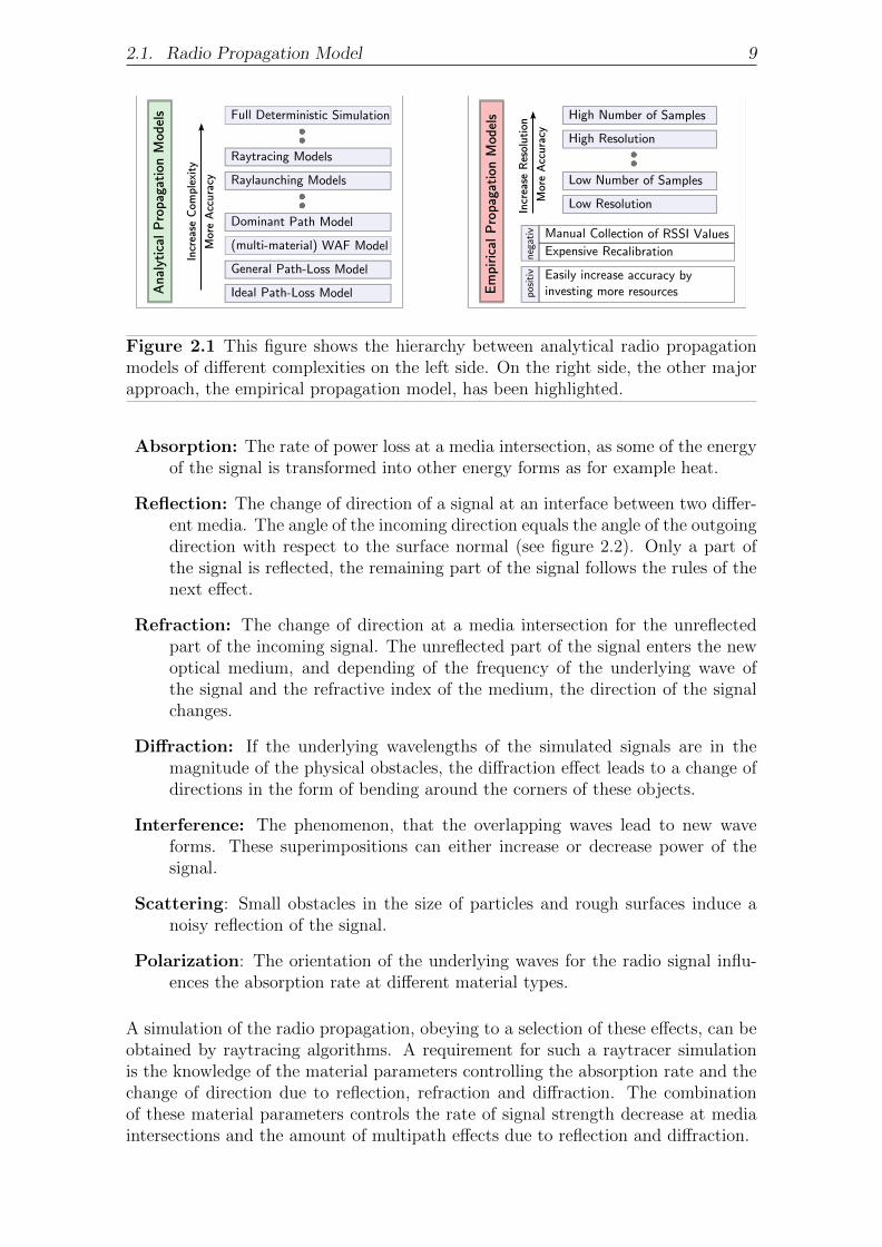
Figure 2.1 This figure shows the hierarchy between analytical radio propagationmodels of different complexities on the left side. On the right side, the other majorapproach, the empirical propagation model, has been highlighted.
Absorption: The rate of power loss at a media intersection, as some of the energyof the signal is transformed into other energy forms as for example heat.
Reflection: The change of direction of a signal at an interface between two differ-ent media. The angle of the incoming direction equals the angle of the outgoingdirection with respect to the surface normal (see figure 2.2). Only a part ofthe signal is reflected, the remaining part of the signal follows the rules of thenext effect.
Refraction: The change of direction at a media intersection for the unreflectedpart of the incoming signal. The unreflected part of the signal enters the newoptical medium, and depending of the frequency of the underlying wave ofthe signal and the refractive index of the medium, the direction of the signalchanges.
Diffraction: If the underlying wavelengths of the simulated signals are in themagnitude of the physical obstacles, the diffraction effect leads to a change ofdirections in the form of bending around the corners of these objects.
Interference: The phenomenon, that the overlapping waves lead to new waveforms. These superimpositions can either increase or decrease power of thesignal.
Scattering: Small obstacles in the size of particles and rough surfaces induce anoisy reflection of the signal.
Polarization: The orientation of the underlying waves for the radio signal influ-ences the absorption rate at different material types.
A simulation of the radio propagation, obeying to a selection of these effects, can beobtained by raytracing algorithms. A requirement for such a raytracer simulationis the knowledge of the material parameters controlling the absorption rate and thechange of direction due to reflection, refraction and diffraction. The combinationof these material parameters controls the rate of signal strength decrease at mediaintersections and the amount of multipath effects due to reflection and diffraction.
10 2. Background
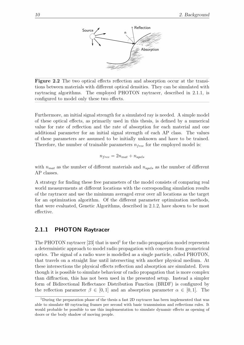
Figure 2.2 The two optical effects reflection and absorption occur at the transi-tions between materials with different optical densities. They can be simulated withraytracing algorithms. The employed PHOTON raytracer, described in 2.1.1, isconfigured to model only these two effects.
Furthermore, an initial signal strength for a simulated ray is needed. A simple modelof these optical effects, as primarily used in this thesis, is defined by a numericalvalue for rate of reflection and the rate of absorption for each material and oneadditional parameter for an initial signal strength of each AP class. The valuesof these parameters are assumed to be initially unknown and have to be trained.Therefore, the number of trainable parameters nfree for the employed model is:
nfree = 2nmat + napcls
with nmat as the number of different materials and napcls as the number of differentAP classes.
A strategy for finding these free parameters of the model consists of comparing realworld measurements at different locations with the corresponding simulation resultsof the raytracer and use the minimum averaged error over all locations as the targetfor an optimization algorithm. Of the different parameter optimization methods,that were evaluated, Genetic Algorithms, described in 2.1.2, have shown to be mosteffective.
2.1.1 PHOTON Raytracer
The PHOTON raytracer [23] that is used1 for the radio propagation model representsa deterministic approach to model radio propagation with concepts from geometricaloptics. The signal of a radio wave is modelled as a single particle, called PHOTON,that travels on a straight line until intersecting with another physical medium. Atthese intersections the physical effects reflection and absorption are simulated. Eventhough it is possible to simulate behaviour of radio propagation that is more complexthan diffraction, this has not been used in the presented setup. Instead a simplerform of Bidirectional Reflectance Distribution Function (BRDF) is configured bythe reflection parameter β ∈ [0, 1] and an absorption parameter α ∈ [0, 1]. The
1During the preparation phase of the thesis a fast 2D raytracer has been implemented that wasable to simulate 60 raytracing frames per second with basic transmission and reflections rules. Itwould probable be possible to use this implementation to simulate dynamic effects as opening ofdoors or the body shadow of moving people.
2.1. Radio Propagation Model 11
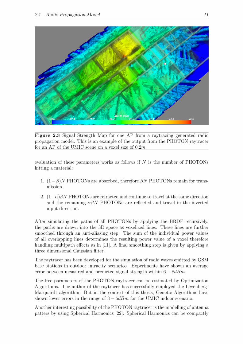
Figure 2.3 Signal Strength Map for one AP from a raytracing generated radiopropagation model. This is an example of the output from the PHOTON raytracerfor an AP of the UMIC scene on a voxel size of 0.2m
evaluation of these parameters works as follows if N is the number of PHOTONshitting a material:
1. (1−β)N PHOTONs are absorbed, therefore βN PHOTONs remain for trans-mission.
2. (1−α)βN PHOTONs are refracted and continue to travel at the same directionand the remaining αβN PHOTONs are reflected and travel in the invertedinput direction.
After simulating the paths of all PHOTONs by applying the BRDF recursively,the paths are drawn into the 3D space as voxelized lines. These lines are furthersmoothed through an anti-aliasing step. The sum of the individual power valuesof all overlapping lines determines the resulting power value of a voxel thereforehandling multipath effects as in [11]. A final smoothing step is given by applying athree dimensional Gaussian filter.
The raytracer has been developed for the simulation of radio waves emitted by GSMbase stations in outdoor intracity scenarios. Experiments have shown an averageerror between measured and predicted signal strength within 6− 8dBm.
The free parameters of the PHOTON raytracer can be estimated by OptimizationAlgorithms. The author of the raytracer has successfully employed the Levenberg-Marquardt algorithm. But in the context of this thesis, Genetic Algorithms haveshown lower errors in the range of 3− 5dBm for the UMIC indoor scenario.
Another interesting possibility of the PHOTON raytracer is the modelling of antennapatters by using Spherical Harmonics [22]. Spherical Harmonics can be compactly
12 2. Background
represented by a set of coefficients for the corresponding functional forms. These co-efficients lead to another set of free parameters, and therefore a larger search-spacefor the Optimization Algorithms. Due to the increased search-space, more train-ing data in form of manual measurements are needed to offset for a phenomenoncommonly referred to as Curse of dimensionality. This phenomenon describes thestatistical problems that arise when the volume of the high-dimensional space in-creases so fast that the training samples become sparsely distributed. Therefore,this technique was not employed in this thesis for the sake of simplicity.
2.1.2 Optimization with Genetic Algorithms
By using an Optimization Algorithm, it is possible to find a set of parameters for amodel that minimizes a given cost function. If the cost function evaluates the error orthe ”quality”of the model, the found parameters are optimal with respect to the costfunction. A set of nfree parameters can also be understood as an element of a nfree-dimensional search-space in R. The cost function that is given by a nfree-parametercontrolled raytracer run can be assumed to be non-linear and non-differentiable dueto the recursive nature of the involved algorithms. Furthermore, it can be safelyassumed, that the function is non-convex leading to multiple local optima.
Of the three evaluated heuristics: Minimum Least Squares, Simulated Annealingand Genetic Algorithms, the last one was capable to generate the best results withrespect to the reached optimum. In a Genetic Algorithm a set of parameters is calleda candidate solution (in the search-space) or simply referred to as an organism. Thesearch for the best set of parameters, also referred to as the fittest organism, is aniterative procedure. The procedure starts with an initialization step where a prede-fined number of organisms are created randomly. Depending on prior informationit is sensible to seed organism in regions of the search-space where optima are moreprobable. In the context of the given optimization problem, it makes sense to useprior knowledge of the estimated power levels of common APs.
After the initialization, the fitness of each organism of the population is evaluatedby calculating the result of the underlying cost function. In the present use casethis means a full raytracer run over all APs and the aggregation of the error at allmeasured locations. Then, the main iteration of the algorithm starts by choosing aproportion of the population for breeding by using the magnitude of the fitness of theorganisms as the selection criteria. Breeding leads to new organism and therefore tothe exploration of the search-space. New organism are breeded by choosing a pair ofparent organisms and crossing over their genes (the nfree-parameters) by selectinggenes randomly from each parent. Additionally to this random selection, a randommutation of the genes can also be applied to allow for a deeper exploration of thesearch-space.
For each breeded organism the fitness will then be evaluated and used to select apredefined number of the fittest children as the new population for the next iterationstep. Different termination conditions can be chosen, like a maximum number ofgenerations/iterations or a minimum needed change toward a minimum cost target.Through this evolutionary inspired selection process the convergence to an, at leastlocal, optimum of the cost function is guaranteed.

2.2. Positioning 13
2.1.3 Error
The error for a radio propagation result will be determined by comparing the corpusof measurements m with the simulation results x for each AP configured with nfree.
RPE(nfree) =1
NapsNlocs
Naps∑a=1
Nlocs∑l=1
||ma,l, xa,l||
where xa,l is the simulation result for AP a and location l. Likewise ma,l is a collectedmeasurement for AP a and location l. Naps is the number of available APs and Nlocs
the size of the training corpus. For ||m, d|| the l1-norm, the absolute delta |m− s| isused. Therefore, the Radio Propagation Error (RPE) is simply the averaged errorover all collected measurements at the different locations in units of dBm.
Another variant of this error that is used in literature is the RMS-RPE. This erroruses the rooted averaged euclidian distance, or the l2-norm, as a metric and is givenby:
RMS −RPE(nfree) =1
NapsNlocs
√√√√Naps∑a=1
Nlocs∑l=1
(ma,l, xa,l)2
The unit of this error is also given by dBm.
2.2 Positioning
The task of Positioning is defined as determining the physical position of a stationarydevice by using information received by the sensors of that device. This information,extracted from some measured signals, is obviously required to be related to thethat position for relevancy. The measured signals are usually obstructed by noisyeffects that come from various sources. The performance of a positioning systemis defined over the error that is given by the distance between the real positionand the estimated one. A well performing positioning model will therefore have tocompensate these noisy effect for minimizing the position error
The source of information that is exploited for positioning in this thesis is givenby measuring the Received-Signal-Strength-Indicator (RSSI) values of available APswith Wi-Fi capable devices. The RSSI value is a measure of the magnitude ofthe electromagnetic field at some physical location. The field is emitted by theantennas of an AP with a known location. The RSSI value is expressed in dBmwhich represents the remaining power of the emitted electromagnetic field in relationto the reference unit of one milliwatt. And explicitly by:
x = 10log10(1000p)
if p is the power at the source of the electromagnetic field given in watt and x is themeasured RSSI value.
Alternate interesting sources of information that are exploited by positioning systemsand that were analysed in recent research [10] are:

14 2. Background
• Time Of Arrival: TOA based methods deduce the distance between transmit-ter and receiver by comparing the timestamp of a packet, originating at thetransmitter with the local timestamp of the receiver. Prior knowledge of thespeed of the transmitted signal combined with the timestamp difference can beused for estimating the covered distance of the signal. A source of error is in-troduced by asynchronous clocks and NLOS conditions that lead to multipatheffects.
• Time Difference Of Arrival: Methods based on TDOA use the difference oftwo TOA measurements emitted by signals at exactly the same time at dif-ferent APs. By using only this difference the requirement of a synchronizedclock between the different transmitting APs and the receiving device can bedropped. But errors induced by timestamp affecting NLOS conditions remain.
• Angle Of Arrival: AOA based methods rely on measuring the angle of theincoming signal at the receiver with directional antennas. A source of erroris induced by NLOS conditions leading to receiving signals of the same APfrom different directions. And another error source in the probable incompleteknowledge of the orientation of the receiver. The requirement of directedantennas at the receiver excludes the use of the commodity WLAN hardwarethat is currently available.
Using the RSSI value as the primary source of information for the positioning systemmakes a good radio propagation model mandatory. Two large sources of errors areexpected. At first, there is the error originating in the unpredictable measurementbehaviour or other noisy effects of the Wi-Fi capable devices. And the other classof errors originates in an inadequate modelling of the radio propagation. By usinga raytracing generated radio propagation model, the reduction of such errors was amajor focus in the presented approach. Especially the inherent modelling of NLOSconditions makes a raytracing approach promising.
Without a raytracer, one has to resort to approximate the dampening effects ofwalls by introducing an attenuation parameter that determines the magnitude ofdampening at a material intersection. Such an attenuation parameter would behighly material dependent. In the raytracer approach, the corresponding modellingis represented by the interaction of the α and β material parameters of the employedbasic BRDF.
Another source of noise with a high impact on the RSSI values is given by the shadoweffect of the human body. Radio waves with 2.4GHZ are easily absorbed by materialswith a high proportion of water. Furthermore, it is expected that location awaredevices are attached or very close to the owner of the device, therefore boosting thisdampening effect.
2.2.1 Techniques
There are different positioning techniques that have been developed by using thementioned information sources. One of the simplest techniques is called ProximitySensing that uses only the identity of the transmitter instead of any distance or angle
2.2. Positioning 15
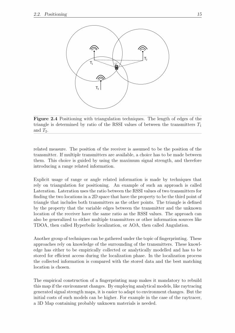
Figure 2.4 Positioning with triangulation techniques. The length of edges of thetriangle is determined by ratio of the RSSI values of between the transmitters T1and T2.
related measure. The position of the receiver is assumed to be the position of thetransmitter. If multiple transmitters are available, a choice has to be made betweenthem. This choice is guided by using the maximum signal strength, and thereforeintroducing a range related information.
Explicit usage of range or angle related information is made by techniques thatrely on triangulation for positioning. An example of such an approach is calledLateration. Lateration uses the ratio between the RSSI values of two transmitters forfinding the two locations in a 2D space that have the property to be the third point oftriangle that includes both transmitters as the other points. The triangle is definedby the property that the variable edges between the transmitter and the unknownlocation of the receiver have the same ratio as the RSSI values. The approach canalso be generalized to either multiple transmitters or other information sources likeTDOA, then called Hyperbolic localization, or AOA, then called Angulation.
Another group of techniques can be gathered under the topic of fingerprinting. Theseapproaches rely on knowledge of the surrounding of the transmitters. These knowl-edge has either to be empirically collected or analytically modelled and has to bestored for efficient access during the localization phase. In the localization processthe collected information is compared with the stored data and the best matchinglocation is chosen.
The empirical construction of a fingerprinting map makes it mandatory to rebuildthis map if the environment changes. By employing analytical models, like raytracinggenerated signal strength maps, it is easier to adapt to environment changes. But theinitial costs of such models can be higher. For example in the case of the raytracer,a 3D Map containing probably unknown materials is needed.
16 2. Background
2.3 Tracking
Tracking is the generalization of the Positioning problem. Whereas Positioning is de-fined as a stationary localization problem, Tracking drops the immobility constraintby allowing the receiving device to move over time. The simplest approach for Track-ing is therefore the sequential execution of a Positioning algorithm with disregardto any structural dependency between the information at different timestamps. Butdoing so, does surely yield an inferior localization result, as the sequential nature ofthe tracking problem is a source of valuable information. Prior knowledge like themaximum walking speed, that is usable as a constraint on the maximum distancebetween two successive positioning results, can easily be exploited.
It is also required to incorporate this source of information in order to offset for themuch larger search-space that is given by the Tracking problem. The search-spacefor the Positioning problem is linearly dependent on the resolution and the size ofthe modelled space. In the worst case that is a high resolution 3D space as usedin the UMIC scene, with around 2 · 106 solutions representing cubes with edge size20cm. In contrast, the solutions for the Tracking problem are sequences of locationswith an additional measurement specific resolution that determines the length ofthat sequence. This length T has an exponential impact on the size of the search-space. An input sequence of signal vectors x with T timeframes, represented as xT1 ,leads to a solutions sequence sT1 . And if the representation of the space is made of Sdisjunct positions, this would induce ST possible solution sequences. Consequently,a brute force search, probably computationally tractable for the singular positioningproblem, has to be excluded as an algorithmic attempt for the Tracking case.
There are two approaches to model the state space of possible locations. Either thespace is assumed to be rasterized or segmented into ”spaces” of interest with someresolution factor for adjusting the granularity, or space is assumed to be dense withreal values for the two or three possible dimensions. The first approach leads modelsbased on Markov chains like Hidden Markov Models (HMM). Since such models havea finite number of states, the computation of a solution involves making decisionsbetween different states by relying on the evaluation of their properties. A majorpart of this thesis studies different aspects of HMM based models.
In contrast, in the second approach a position, given in real values, is updatedby some function configured with prior knowledge of the environment or of thebehaviour of the moving person. The evaluation of this function results in the next-best real valued position. Examples of this approach can be found in the form ofParticle Filters or in the different forms of Kalman Filters.
2.3.1 Mobility Models
The different approaches for tackling the sequential nature of the tracking problemhave in common, that they use prior information of the shape of the environment orprior knowledge of the rules that a moving device has to obey. There are multiplesources for extracting such information.
A deterministic mobility model can be employed, if the speed and acceleration of amoving device are available. Combining such information with the laws of physics,
2.3. Tracking 17
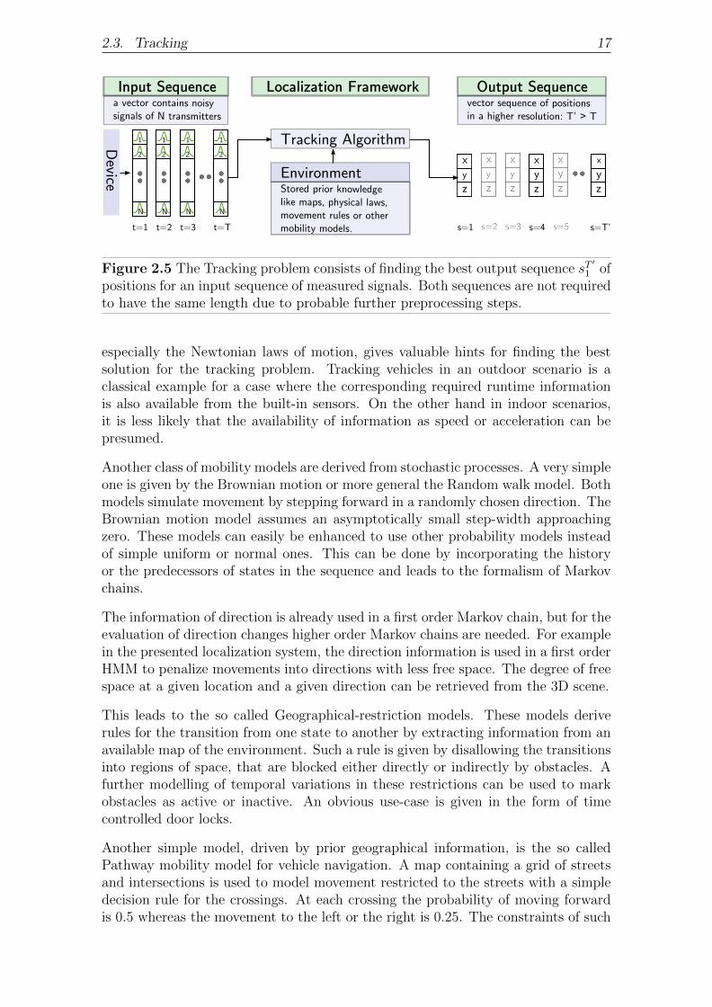
Figure 2.5 The Tracking problem consists of finding the best output sequence sT′
1 ofpositions for an input sequence of measured signals. Both sequences are not requiredto have the same length due to probable further preprocessing steps.
especially the Newtonian laws of motion, gives valuable hints for finding the bestsolution for the tracking problem. Tracking vehicles in an outdoor scenario is aclassical example for a case where the corresponding required runtime informationis also available from the built-in sensors. On the other hand in indoor scenarios,it is less likely that the availability of information as speed or acceleration can bepresumed.
Another class of mobility models are derived from stochastic processes. A very simpleone is given by the Brownian motion or more general the Random walk model. Bothmodels simulate movement by stepping forward in a randomly chosen direction. TheBrownian motion model assumes an asymptotically small step-width approachingzero. These models can easily be enhanced to use other probability models insteadof simple uniform or normal ones. This can be done by incorporating the historyor the predecessors of states in the sequence and leads to the formalism of Markovchains.
The information of direction is already used in a first order Markov chain, but for theevaluation of direction changes higher order Markov chains are needed. For examplein the presented localization system, the direction information is used in a first orderHMM to penalize movements into directions with less free space. The degree of freespace at a given location and a given direction can be retrieved from the 3D scene.
This leads to the so called Geographical-restriction models. These models deriverules for the transition from one state to another by extracting information from anavailable map of the environment. Such a rule is given by disallowing the transitionsinto regions of space, that are blocked either directly or indirectly by obstacles. Afurther modelling of temporal variations in these restrictions can be used to markobstacles as active or inactive. An obvious use-case is given in the form of timecontrolled door locks.
Another simple model, driven by prior geographical information, is the so calledPathway mobility model for vehicle navigation. A map containing a grid of streetsand intersections is used to model movement restricted to the streets with a simpledecision rule for the crossings. At each crossing the probability of moving forwardis 0.5 whereas the movement to the left or the right is 0.25. The constraints of such
18 2. Background
a model can easily be projected into an indoor scenario, but here, also allowing achange in the opposite direction should also be considered.
The last class of mobility models rely on exploiting the behaviour of multiple syn-chronously moving devices. Therefore, they are called Group mobility models. It isfor example plausible to assume, that vehicles on a street that are near to each other,have correlated speed and direction properties. The same holds true for swarms ofanimals or human movement on crowded places.
2.3.2 Error
The error of a Tracking result sT1 can be given in the form of the Root Mean SquareTracking Error (RMS-TE). The RMS-TE between the correct sequence of positionsrT1 and the estimated sequence sT1 is defined as:
RMS − TE(sT1 , rT1 ) =
√∑Tt=1(||rt, st||)2
T
with ||rt, st|| as the 2D or 3D euclidian distance between the real positions rt andst. The performance of a localization system can be given by evaluating the errorover multiple tracking attempts stored in an evaluation corpus C.
RMS − LE(C) =
√√√√ 1
N
N∑c=1
1
Tc
Tc∑t=1
(||rc,t, sc,t||)2
where Tc is the length of a sample from the corpus. This error can also be evaluatedfor the positioning problem by assuming that Tc = 1 for all pseudo-paths of thecorpus. In literature a variant of this error is also given by using the simpler l1-norm:
LE(C) =1
N
N∑c=1
1
Tc
Tc∑t=1
|rc,t − sc,t|
This error should be referred to as the averaged Localization Error evaluated ona collected corpus of tracked paths. All three error variants are given in the unitmeter.
2.4 Bayesian Pattern Recognition
For understanding the approaches to the localization problem, that are presented inthe following sections, a general understanding of the basic principles of Bayesianinference is needed. Therefore, a short introduction into this very popular approachto the problem of machine learning and pattern recognition is given.
In Bayesian inference, the Bayes theorem is used to compute how the degree of beliefin a proposition changes due to available evidence. In the context of RSSI informa-tion based localization, the proposition is: ”The device is there.” with the evidence:”It has received these RSSI readings”. Since such a proposition is inherently a de-cision for a state2 in a however modelled environment, it will be represented by s.
2Another convention for formalizing the concept of the proposition is given by the notion of aclass that will be decided upon.
2.4. Bayesian Pattern Recognition 19
The simplest state space is defined by the 2-state case: ”The received email text iseither spam or ham”. In this minimal example, the previously mentioned evidenceis a representation of the text in a machine processable form. Such a form of theevidence is commonly called Feature Vector and should be denoted as x.
For the ”decision making process”, that should be called Decision Rule, it would bebeneficial to have a measure of the quality of the different possible decisions, thedifferent possible states under the feature vector represented evidence. In Bayesianinference this measure is given by the joint probability between the state s and thefeature vector x with:
p(x, s)
which evaluates under the definitions of probability theory to a scalar value in therange [0..1]. Furthermore, if x and s are conditionally independent, the joint proba-bility can be factored into the two conditional forms that are essential for the Bayestheorem:
p(x, s) = p(x|s)p(s) = p(s|x)p(x)
Under the Bayes theorem, the interpretation of the probabilities p(x|s), p(s) andp(s|x) is indicated by their commonly used names. p(s|x) is called the posteriorprobability as it represents the belief that the state follows the evidence given byx. p(s) is the prior probability and represents an evidence independent knowledgeabout the probability how often the state s will be observed. And finally, p(x|s) is thestate-conditional probability that represents the probability to observe the evidence xunder assumption that the environment is in state s. p(x), the probability to observea specific evidence, has not been given a dedicated name as it will be unimportantfor the sought Decision Rule.
The Decision Rule should obviously lead to a high quality decision. This shouldtherefore be the decision with the maximum joint probability. By this reasoning,the Bayes Decision Rule rbayes : x→ s is defined as:
rbayes(x) = argmaxs
p(x, s)
which factors according to the laws of conditional probabilities into:
rbayes(x) = argmaxs
[p(s|x)p(x)]
= argmaxs
[p(s|x)] , since argmaxs
is independent of p(x)
This is an intuitive result. A decision that is based on the posterior probabilityleads to the same result as using the joint probability. But it is still unknown howto obtain the posterior p(s|x). Therefore, the Bayes theorem will be used again:
p(s|x) =p(x|s)p(s)p(x)
Inserting the factored posterior into the Decision Rule:
rbayes(x) = argmaxs
[p(x|s)p(s)p(x)
]= argmax
s[p(x|s)p(s)] , since argmax
sis independent of p(x)

20 2. Background
This is not an intuitive Decision Rule any more, but probability models for p(x|s)and p(s) can be learned from the environment. The prior p(s) is a discrete PDF,due to the discrete nature of the states3, that can be determined by simple countingof the occurrences of s.
Modelling the state-conditional distribution p(x|s) is more complicated. The vectorspace of x, the numerical representation of the evidence, can have manifold shapes.It can be of categorical nature leading to a discrete PDF, or, if it represents physicalmeasurements it will become a continuous one. The analytical choice of the formof the PDF, whether it is a multi-variate Gaussian, a mixture density or anothercomplex distribution, can be termed: to apply model assumptions. If the prioranalysis has lead to a p(x|s) that is modelled according to the true nature of theenvironment, the free parameters of the model need to be determined. Similar tolearning the structure of the prior p(s), the parameters of p(x|s) can be learnedfrom the environment. But due to the coupling of s and x, special state-annotatedevidence-data is needed. Ignoring the problem of gathering this data, parameterestimation techniques like Maximum-Likelihood can then be applied to the set oftraining samples. If p(x|s) is modelled as a Gaussian, this results in estimating themean and the variance.
Summarizing the results: The Bayes Decision Rule conducts a search for the states with the maximum posterior probability p(s|x) for an observed feature vector x.The Bayes Decision Rule is therefore a function with input given by some measuredevidence x leading to the output of the most probable state s of the environment.Instead of directly evaluating the posterior probability p(s|x), the prior p(s) andstate-conditional p(x|s) are employed as they can be learned from the environment.p(s) can be easily learned by counting. And for p(x|s), suitable model assumptionsmust be chosen and the free parameters of the model need to be trained.
If these concepts are applied to the positioning problem with RSSI measurements,this leads to the following example model:
1. A state s is an enumerable region of space, a location.
2. The feature vector x is the jointly received vector of RSSI values for differentAPs.
3. p(s) is the probability to be in a specific location. In a geographically-restrictedmobility-model, p(s) would be zero for unreachable regions.
4. p(x|s) is the probability to receive the measurements x at the location s. p(x|s)can be modelled as a multi-variate Gaussian, with a mean vector that repre-sents the anticipated AP-specific RSSI values at the location s. Assumingequal noise over all APs, a signal variance of around 5dBm will be chosen.
5. The AP-specific means of p(x|s) will be obtained from a radio propagationmodel.
3It is possible to assume a continuous state space as well, but this has not been done forsimplicity.
2.5. Hidden Markov Models 21
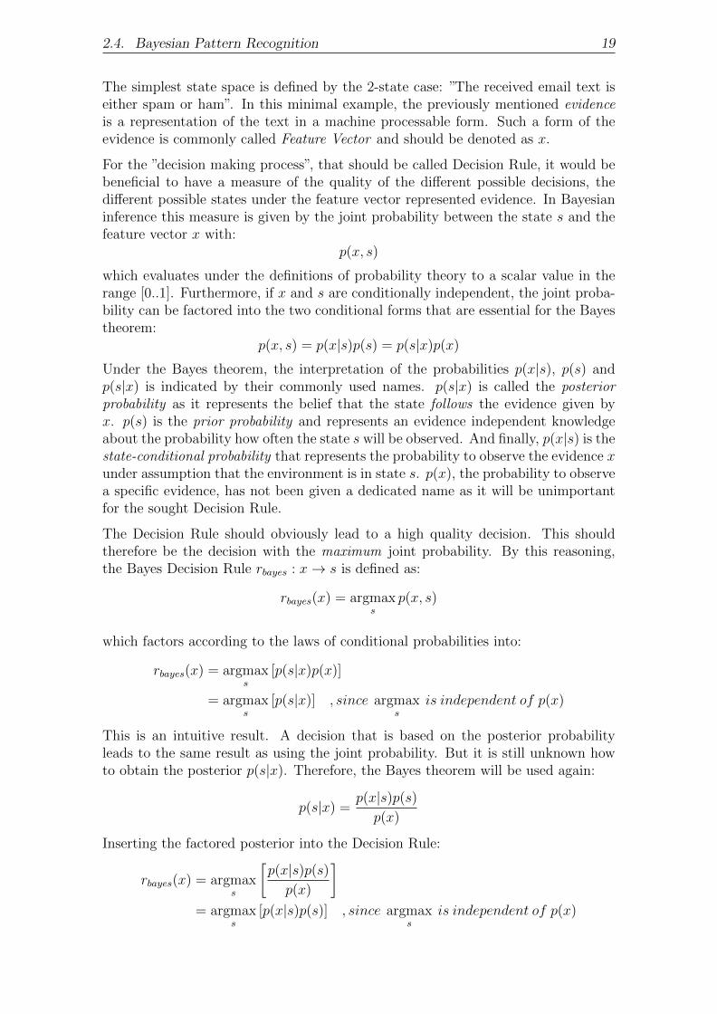
Figure 2.6 Markov chain with a (0, 1, 2) transition model. The choice of the futurestate depends only on the present state.
For a new RSSI vector observation x the Bayes Decision Rule is used to decide for themost probable location s that explains the observation. This means evaluating theposteriors p(s|x) for all all locations, and selecting the location s with max (p(s|x)).Due to the unavailability of a direct form of p(s|x), the maximization is carried outover the known prior p(s) and the state-conditional p(x|s).
If the prior p(s) is assumed to be constant for all s, then this will lead to the LMSEbased localization approach that will be described in section 2.7.
2.5 Hidden Markov Models
The Hidden Markov Model approach to the localization problem leads to the firstalgorithm that is based on the principles of Bayesian inference. But before thenature of the state-conditional is discussed, the formalism of the Markov Chain isintroduced to derive the source for the prior probability.
The process of movement through space can be modelled as a Markov chain. Eachpossible discrete position in space, their number depends on the rasterization res-olution, translates to a state in the Markov chain. A Markov chain is a sequenceof states in a stochastic process where the Markov property holds. The Markovproperty refers to the memorylessnes of the process, that is given by the constraintthat a future state depends only on the present state and ignores all other precedinghistory.
Such a Markov chain is parametrized by transition probabilities. The transitionprobabilities form a discrete probability distribution. A transition is the pair s′ → s.The conditional probability for a transition, the probability that the future state sfollows after the present state s′ is given by p(s|s′). The normalization constraint ofa PDF holds: ∑
s
p(s|s′) = 1, ∀s′
A special transition model, allowing only three predecessor states, is the (0, 1, 2)-model (see figure 2.6) that is defined by:
2∑i=0
p(s+ i|s) = 1
with s + i representing a state index as the notation st is used for indexing overtime frames. The (0, 1, 2)-model is used for time alignment, that has the goal for
22 2. Background
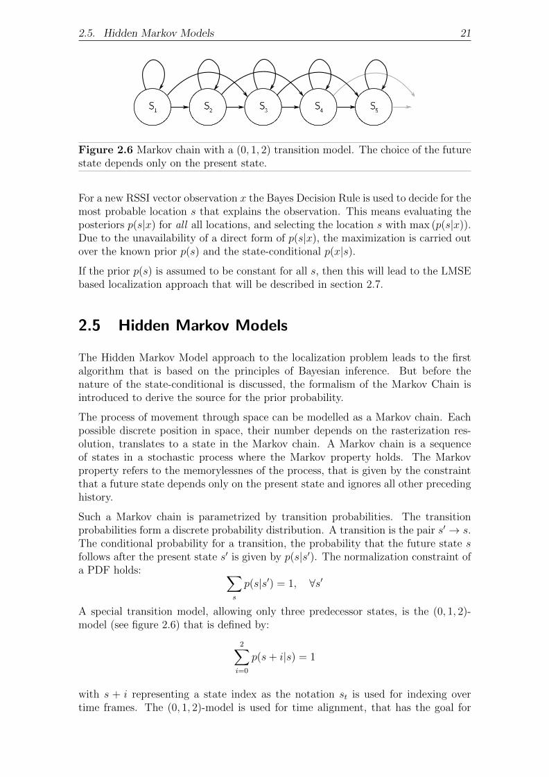
Figure 2.7 In a Hidden Markov Model the states are not directly observable. Butthe output of the states can be measured as sequence of feature vectors. From theseobservations the best matching state sequence sT1 can be recovered.
compensating distortions in the speed of the stochastic process. If the process isonly developing slowly, for example a slowly moving localization target, more 0-transitions can be used. In a 0-transition the process remains in the present state.The opposite effect have 2-transitions. They are employed to model acceleratedphases of the stochastic process. Elevating the one dimensional (0, 1, 2)-model intothe three dimensional localization space with six degrees of freedom leads to therather clumsy notation of ((0, 1, 2)1, (0, 1, 2)2, .., (0, 1, 2)6)-model. By combining the0-transitions and counting only the number of predecessors on each dimension thisshould be called (5, 5, 5)-model. The (5, 5, 5)-model is parametrized by 125 possibletransitions for each state.
In a Hidden Markov Model (HMM), the states of the Markov chain are not directlyobservable. But the output of the states, also called the emission of the states,is visible. The visible emission x is coupled to the hidden state s through theprobability distribution p(x|s). Therefore, by observing a sequence of measurementsand relating them to the emission probabilities, the HMM can be used for assigningprobabilities to different hypothesized hidden sequences which on their part are listsof locations.
This emission probability p(x|s) represents the state-conditional probability in theBayesian approach and has to be learned from the environment. In the context oflocalization, the state s represents a position in space. Therefore, it is understoodas a model for the probability to receive a special signal constellation at a givenposition. Emission probabilities are often modelled as multivariate Gaussians ormore complex mixture densities. The chosen model properties for the emissions inthis thesis are discussed in the later section 2.5.4, where the simplification of thementioned Gaussians is of concern.
2.5. Hidden Markov Models 23
2.5.1 Decision Rule
Finding the best matching sequence of positions sT1 for a given sequence of mea-surements xT1 is defined under the Bayesian approach by finding the maximum jointprobability:
sT1 = argmaxsT1
p(xT1 , sT1 )
applying the product rule leads to:
sT1 = argmaxsT1
T∏t=1
p(xt, st|xt−11 , st−11 )
In the HMM formalism, there is no condition on the previous emission vectors. Theycan be dropped:
sT1 = argmaxsT1
T∏t=1
p(xt, st|st−11 )
and there is only a dependency on the previous state (first-order Markov):
sT1 = argmaxsT1
T∏t=1
p(xt, st|st−1)
= argmaxsT1
T∏t=1
p(st|st−1) · p(xt|st−1, st)
= argmaxsT1
T∏t=1
p(st|st−1) · p(xt|st)
Therefore, calculating the probability of a sequence sT1 is reduced to iteratively com-bining the transition probability of a jump and the emission probability for a mea-sured signal vector xt at the jump destination. This is a very cheap operation, sop(xT1 , s
T1 ) can be determined in fractions of microseconds.
With this representation, a solution for the maximization can already be foundwith a brute force approach. The product has to be evaluated for all possible statesequences sT1 . But with N possible transitions from one state s′ into another s, thecomputational complexity is given by NT solutions. This makes a brute force searchintractable.
2.5.2 Viterbi Algorithm
The Viterbi Algorithm is an efficient dynamic programming algorithm for finding themost probable state sequence sT1 for an observed vector sequence xT1 . The Algorithmexploits the memorylessnes of the model that is induced by the Markov property.The Algorithm is defined as a set of recursive equations starting with:
Q(t, s) := maxst1:st=s
t∏τ=1
p(xτ , sτ |sτ−1)
24 2. Background
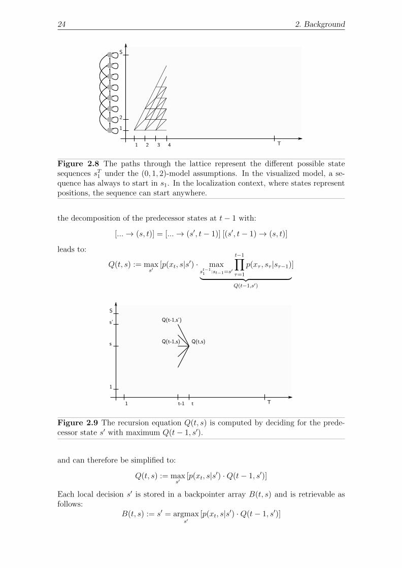
Figure 2.8 The paths through the lattice represent the different possible statesequences sT1 under the (0, 1, 2)-model assumptions. In the visualized model, a se-quence has always to start in s1. In the localization context, where states representpositions, the sequence can start anywhere.
the decomposition of the predecessor states at t− 1 with:
[...→ (s, t)] = [...→ (s′, t− 1)] [(s′, t− 1)→ (s, t)]
leads to:
Q(t, s) := maxs′
[p(xt, s|s′) · maxst−11 :st−1=s′
t−1∏τ=1
p(xτ , sτ |sτ−1)︸ ︷︷ ︸Q(t−1,s′)
]
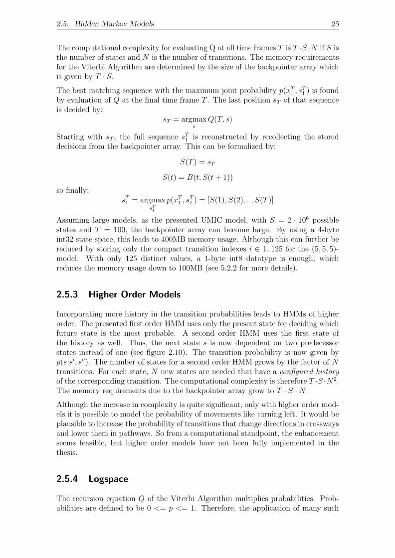
Figure 2.9 The recursion equation Q(t, s) is computed by deciding for the prede-cessor state s′ with maximum Q(t− 1, s′).
and can therefore be simplified to:
Q(t, s) := maxs′
[p(xt, s|s′) ·Q(t− 1, s′)]
Each local decision s′ is stored in a backpointer array B(t, s) and is retrievable asfollows:
B(t, s) := s′ = argmaxs′
[p(xt, s|s′) ·Q(t− 1, s′)]
2.5. Hidden Markov Models 25
The computational complexity for evaluating Q at all time frames T is T ·S ·N if S isthe number of states and N is the number of transitions. The memory requirementsfor the Viterbi Algorithm are determined by the size of the backpointer array whichis given by T · S.
The best matching sequence with the maximum joint probability p(xT1 , sT1 ) is found
by evaluation of Q at the final time frame T . The last position sT of that sequenceis decided by:
sT = argmaxs
Q(T, s)
Starting with sT , the full sequence sT1 is reconstructed by recollecting the storeddecisions from the backpointer array. This can be formalized by:
S(T ) = sT
S(t) = B(t, S(t+ 1))
so finally:sT1 = argmax
sT1
p(xT1 , sT1 ) = [S(1), S(2), .., S(T )]
Assuming large models, as the presented UMIC model, with S = 2 · 106 possiblestates and T = 100, the backpointer array can become large. By using a 4-byteint32 state space, this leads to 400MB memory usage. Although this can further bereduced by storing only the compact transition indexes i ∈ 1..125 for the (5, 5, 5)-model. With only 125 distinct values, a 1-byte int8 datatype is enough, whichreduces the memory usage down to 100MB (see 5.2.2 for more details).
2.5.3 Higher Order Models
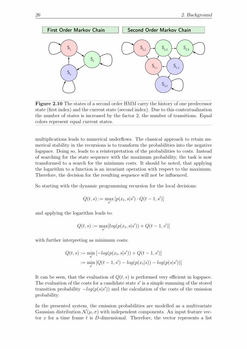
Incorporating more history in the transition probabilities leads to HMMs of higherorder. The presented first order HMM uses only the present state for deciding whichfuture state is the most probable. A second order HMM uses the first state ofthe history as well. Thus, the next state s is now dependent on two predecessorstates instead of one (see figure 2.10). The transition probability is now given byp(s|s′, s′′). The number of states for a second order HMM grows by the factor of Ntransitions. For each state, N new states are needed that have a configured historyof the corresponding transition. The computational complexity is therefore T ·S ·N2.The memory requirements due to the backpointer array grow to T · S ·N .
Although the increase in complexity is quite significant, only with higher order mod-els it is possible to model the probability of movements like turning left. It would beplausible to increase the probability of transitions that change directions in crosswaysand lower them in pathways. So from a computational standpoint, the enhancementseems feasible, but higher order models have not been fully implemented in thethesis.
2.5.4 Logspace
The recursion equation Q of the Viterbi Algorithm multiplies probabilities. Prob-abilities are defined to be 0 <= p <= 1. Therefore, the application of many such
26 2. Background
Figure 2.10 The states of a second order HMM carry the history of one predecessorstate (first index) and the current state (second index). Due to this contextualizationthe number of states is increased by the factor 2, the number of transitions. Equalcolors represent equal current states.
multiplications leads to numerical underflows. The classical approach to retain nu-merical stability in the recursions is to transform the probabilities into the negativelogspace. Doing so, leads to a reinterpretation of the probabilities to costs. Insteadof searching for the state sequence with the maximum probability, the task is nowtransformed to a search for the minimum costs. It should be noted, that applyingthe logarithm to a function is an invariant operation with respect to the maximum.Therefore, the decision for the resulting sequence will not be influenced.
So starting with the dynamic programming recursion for the local decisions:
Q(t, s) := maxs′
[p(xt, s|s′) ·Q(t− 1, s′)]
and applying the logarithm leads to:
Q(t, s) := maxs′
[log(p(xt, s|s′)) +Q(t− 1, s′)]
with further interpreting as minimum costs:
Q(t, s) := mins′
[−log(p(xt, s|s′)) +Q(t− 1, s′)]
:= mins′
[Q(t− 1, s′)− log(p(xt|s))− log(p(s|s′))]
It can be seen, that the evaluation of Q(t, s) is performed very efficient in logspace.The evaluation of the costs for a candidate state s′ is a simple summing of the storedtransition probability −log(p(s|s′)) and the calculation of the costs of the emissionprobability.
In the presented system, the emission probabilities are modelled as a multivariateGaussian distribution N (µ, σ) with independent components. An input feature vec-tor x for a time frame t is D-dimensional. Therefore, the vector represents a list
2.5. Hidden Markov Models 27
of RSSI readings from D Access Points. The RSSI readings are assumed to bestochastically independent. The analytical form of p(x|s) is given by:
p(x|s) = p(x1, ..., xd, ..., xD|s) =D∏d=1
p(xd|s)
=1∏D
d=1
√2πσ2
sd
exp
[−1
2
D∑d=1
(xd − µsdσsd
)2]
The next model assumption is introduced in the form of a constant pooled variancefor all states and dimensions. This leads to a further simplification of the emissionmodel:
p(x|s) =1
C1
exp
[−C2
2
D∑d=1
(xd − µsd)2]
transforming the equation with the negative logarithm:
−log(p(x|s)) =C2
2
D∑d=1
(xd − µsd)2 + log(C1)
insertion into the recursion equation and dropping the constants C1, C2 due to theminimization leads to:
Q(t, s) := mins′
[Q(t− 1, s′) +D∑d=1
(xtd − µsd)2 − log(p(s|s′))]
Thus, in logspace the Gaussian modelled emission probability is simplified to adistance calculation between xtd and the stored µsd components.
2.5.5 Pruning
Pruning, also known as Beam Search, is a heuristic approach to make the ViterbiAlgorithm more efficient. The basic idea is to skip the evaluation of Q(t, s) that aredetermined to be unlikely with respect to the global optimum. Therefore, findingthe global optimum, the most probable sequence sT1 , is not guaranteed any more.Loosing the global optimum will be more probable if the pruning is too aggressiveand the number of evaluated states becomes too low.
There are two pruning strategies. The first strategy discards unlikely hypothesesif their probability drops below a threshold that is determined by the probabilityQtop(t) of the top hypothesis:
Qtop(t) = maxsQ(t, s)
by introducing a factor f , the state hypothesis (s, t) is pruned if:
Q(t, s) < f ·Qtop(t)
With this strategy, the number of unpruned states is variable for each time frame t.
The other strategy induces a hard limit N on the number of unpruned states. Duringthe evaluation of Q(t, s) for a given time frame, the top-N states are collected forensuring their further processing in the next t + 1 time frame. Due to the simplermemory management, this strategy has been chosen in this thesis.
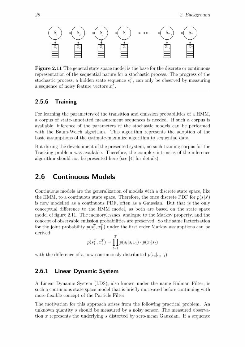
28 2. Background
Figure 2.11 The general state space model is the base for the discrete or continuousrepresentation of the sequential nature for a stochastic process. The progress of thestochastic process, a hidden state sequence sT1 , can only be observed by measuringa sequence of noisy feature vectors xT1 .
2.5.6 Training
For learning the parameters of the transition and emission probabilities of a HMM,a corpus of state-annotated measurement sequences is needed. If such a corpus isavailable, inference of the parameters of the stochastic models can be performedwith the Baum-Welch algorithm. This algorithm represents the adoption of thebasic assumptions of the estimate-maximize algorithm to sequential data.
But during the development of the presented system, no such training corpus for theTracking problem was available. Therefore, the complex intrinsics of the inferencealgorithm should not be presented here (see [4] for details).
2.6 Continuous Models
Continuous models are the generalization of models with a discrete state space, likethe HMM, to a continuous state space. Therefore, the once discrete PDF for p(s|s′)is now modelled as a continuous PDF, often as a Gaussian. But that is the onlyconceptual difference to the HMM model, as both are based on the state spacemodel of figure 2.11. The memorylessnes, analogue to the Markov property, and theconcept of observable emission probabilities are preserved. So the same factorizationfor the joint probability p(sT1 , x
T1 ) under the first order Markov assumptions can be
derived:
p(sT1 , xT1 ) =
T∏t=1
p(st|st−1) · p(xt|st)
with the difference of a now continuously distributed p(st|st−1).
2.6.1 Linear Dynamic System
A Linear Dynamic System (LDS), also known under the name Kalman Filter, issuch a continuous state space model that is briefly motivated before continuing withmore flexible concept of the Particle Filter.
The motivation for this approach arises from the following practical problem. Anunknown quantity s should be measured by a noisy sensor. The measured observa-tion x represents the underlying s distorted by zero-mean Gaussian. If a sequence

2.6. Continuous Models 29
of measurements is available in the form of xT1 , the hidden value of s can be easilyestimated by averaging of the measurements.
The problem will again become more complex if the quantity s is allowed to changeover time. An obvious approach would be to use some form of historical averageof the last measurements to estimate the current true value of s. But how farshould that evaluated window of measurements reach back? If the value for s ischanging slowly over time, a large window capturing a lot of valuable informationis appropriate. But if the value for s is changing fast, this leads to averaging overhigh variety information and therefore introduce a new form of error. Here, a shortmoving average window is better. This approach can be made more complicated byintroducing a weighed average of the history, probably giving more recent ones moreweight. This reasoning relates to the need for state-conditional probabilities p(x|s),now the transitions will be investigated.
The other source of information, the transition probability p(s|s′) is modelled by anon-stationary multivariate linear-Gaussian distribution:
p(s|s′) = N (s|As′, B)
where A is the linear transformation representing the movement vector and B theinitial mean and variance. The requirement of a linearly changing state sequence isgiven by the need for integration instead of summing during finding the marginalsof p(xT1 |sT1 ). A similar restriction is enforced on the emission probabilities. Onlysimple PDFs like Gaussians are allowed for p(x|s). Mixtures densities lead also toproblems during integration due to their contained summations.
These limitations were addressed by the introduction variants of that approach. Forexample, the extended Kalman filter [14] or the also preseneted Particle Filter, dropsthe restriction of linearity in the state changes.
For a more detailed introduction of the LDS technique, it should be referred to [21]and [4].
2.6.2 Particle Filter
One of the more recent approaches to the tracking problem, that was also evaluatedin this thesis, is given by the Particle Filter (PF) [7]. The model is a responseto the problem that estimating the non-linear movement of a person in an indoorlocalization scenario with the linear Kalman Filter is prone to fail. The concepts ofthe PF are based on the idea to sample the posterior distribution p(st|xt) directlyfor a given time frame t. In the HMM formalism, this posterior distribution isapproximated by the recursion equation Q(s, t). And due to the enumerability ofthe discrete states, the Viterbi Algorithm is able to compute p(st|xt) and can thusdecide locally for the state st with maximum probability. The goal of this procedurecan also be described as a marking of the most probable states or locations given anobserved measurement sequence.
The same marking of probable states in a continuous space is conducted if p(st|xt)is sampled under the conditions of the observations. By generating enough samples,the best state hypothesis will get the most probability mass. This is in a way an

30 2. Background
analogue to the remaining unpruned states of the pruning HMM. The unprunedstates at a time frame t determine the new set of unpruned states at t + 1 byevaluation of a new xt. In the Particle Filter, the set of samples at a time frame tis equivalently used to generate the new set of samples for t+ 1 with respect to thenew observations of xt.
The sampling process is defined recursively4. Let {s(l)t } be set of samples with
cardinality L for a timeframe t and {s(l)0 } an initial set of samples that are drawn
from a p(s0) distribution. Then, the sampling weights {w(l)t } are defined by:
w(l)t =
p(xt|s(l)t )∑Lm=1 p(xt|t
(m)t )
The weight for a sample is therefore computed from the emission probabilitiesp(xt|st) that are obtained from the radio propagation models. The weights sat-
isfy the normalization constraint∑
l w(l)t = 1 and are in the range 0 ≤ w
(l)t ≤ 1.
They can be understood as a way to explain the importance of each sample underthe current observation xt. The posterior p(st|xt) is represented by the combinationof the samples and the corresponding weight for each sample. The next posteriorp(st+1|xt) is defined by combining the weights of t and the transition probabilitiesp(s|s′) to the following mixture:
p(st+1|xt) =L∑l=1
w(l)t p(st+1|st)
By drawing new samples {w(l)t+1} from this distribution, the recursive step is com-
pleted. Therefore, the algorithm can be interpreted as to switch between two modes.At first, the weight of the samples under the observation x is determined by usingthe stored p(x|s). The weight defines the number of new samples that are spawnedfrom this sample. In the context of this thesis: If the sample represents a very prob-able location for the RSSI readings, the sample location is used as a major sourcefor the next set of samples.The following set of samples is then generated by spawning the appropriate numberof samples at each source into the most probable direction/distance given by thetransition probability p(s|s′).
2.7 Least Mean Squared Error
Another localization method, that has been prominently used due to it’s simplisticprinciples, is given by the so called Least Mean Squared Error (LMSE). Contrary tothe HMM and the PF based approaches, the method ignores the sequential natureof the measurements and is therefore not based on the state space model of figure2.11. The basic idea is given by comparing the RSSI reading of the D-dimensionalmeasurement vector x with all location s annotated measurements ys of a databaserepresenting the prior knowledge of the distribution. The LMSE uses the euclidian
4A more detailed presentation of the PF can be found in [4].
2.8. Summary 31
distance for the comparison and decides for the location with the least distance. TheLMSE decision rule rlmse : x→ s is thus defined as:
rlmse(x) = argmins
[1
D
D∑d=1
(xd − ysd)2]
= argmins
D∑d=1
(xd − ysd)2
The method is derived from the Bayes Decision Rule that has been introduced insection 2.4:
rbayes(x) = argmaxs
[p(x|s)p(s)]
All locations are equally probable, and the calculation is done in logspace:
rbayes(x) = argmaxs
[log(p(x|s))]
The location-conditional p(x|s) is modelled as a Gaussian with independent compo-nents: p(x|s) ∼ N (µ, σ). Furthermore, by assuming a constant pooled variance overall locations and removing the constant coefficients of the Gaussian5, this leads to:
rbayes(x) = argmaxs
[−
D∑d=1
(xd − µsd)2]
= argmins
D∑d=1
(xd − µsd)2
Therefore, under the given assumptions for p(x|s) and if ys = µs the followingequality holds:
rlmse(x) = rbayes(x)
2.8 Summary
A thorough introduction into the general principles that are employed to approachthe localization problem and the radio propagation modelling was given. TheBayesian approach to the pattern recognition problem was introduced and threealgorithms, the HMM, the PF and the LMSE technique were derived. For the topicof radio propagation, the basic background information needed for understanding theprimary physical effects that influence the RSSI signal distribution were presented.Building on that foundations, a brief overview over the mechanics of employed PHO-TON system was given.
5A similar transformation into logspace has been done with the HMM emission probabilitiesp(x|s) in section 2.5.4. A pooled variance, has been used there as well.
32 2. Background
The Tracking problem, the search for the best matching sequence sT1 for a given xT1 ,has been shown to be addressable with a number of different algorithms. The firstone shown, was derived from the concepts of Hidden Markov Models. The modelassumptions of a HMM, especially the memorylessnes due to the Markov property,make use of efficient dynamic programming algorithms for finding sT1 possible. Thecomputations in the Viterbi Algorithm were further simplified by moving the prob-abilities into logspace and assuming a constant pooled variance on the emissionprobabilities. The final computations contain only summations, memory lookupsfor stored probabilities and a distance calculation between xt and the stored RSSIvalues of the radio propagation model. Since the computations for Q(s, t) are sim-ple, the implemented system can process around 5 ·106Q(s, t) per second on currenthardware. The proposed Pruning technique leads to a further speed-up of aroundone order of magnitude.
The other two presented algorithms are the LMSE and the Particle Filter. Thelatter is similar to the HMM as it is also derived from the state space model offigure 2.11. Whereas, the LMSE approach ignores the additional knowledge givenby the history of the RSSI readings, the HMM/PF respect the sequential natureof the problem by modelling transition probabilities. As becomes observable duringthe later evaluation of the three algorithms, that incorporating this knowledge aboutthe stochastic process leads to significantly reduced localization error rates.
The Positioning problem will be understood as a special case of the Tracking prob-lem. The same algorithmic designs are used for finding solutions. Although in theworst case, a positioning attempt contains only data from one time frame withoutexploitable history. In this special case the LMSE approach does represent the mostefficient solution. But it can be assumed, that in the presented use-case of Wi-Fibased positioning, the signal stream is easily adaptable to employ sequential data.
3Related Work
This chapter gives an overview over related research that has been conducted oneither modelling the radio propagation of AP transmitters in section 3.1 and overlocalization algorithms exploiting this information in section 3.2. Since the largerfocus of this thesis was placed on the localization algorithms, especially the HMMand PF approach, the latter section is formed more broadly.
An historically important project, especially for RSSI based indoor localization sys-tems, is given by the RADAR [2] framework. This framework combines the basicmethodology, the appliance of a radio propagation model (the WAF model) to alocalization algorithm (specifically the LMSE), that was also used in this thesis andother related works.
3.1 Radio Propagation
The two major approaches for the radio propagation model are either manuallybuilding a database of RSSI readings or using an analytical model for simulatingthe radio propagation. Historically, the former approach has been used more promi-nently as it gives a simple procedure to build a map of RSSI values for an indoorscene. The latter, the modelling by reasoning about the physical nature of the radiopropagation, is a response to the expensive nature of the labour-intensive manualcollection and leads to ray tracing based models of different complexities. A selectionof localization systems that have employed analytical models based on 2D or 3D-raytracers are presented here. The following aspects of the systems are highlighted:
1. How detailed is the simulation of the physical effects at the intersection pointsbetween rays and scene geometry?
2. Is the transmitter of the signal a simple isotropic model or more complex?
3. What is the source for the 2D/3D-scene geometry?
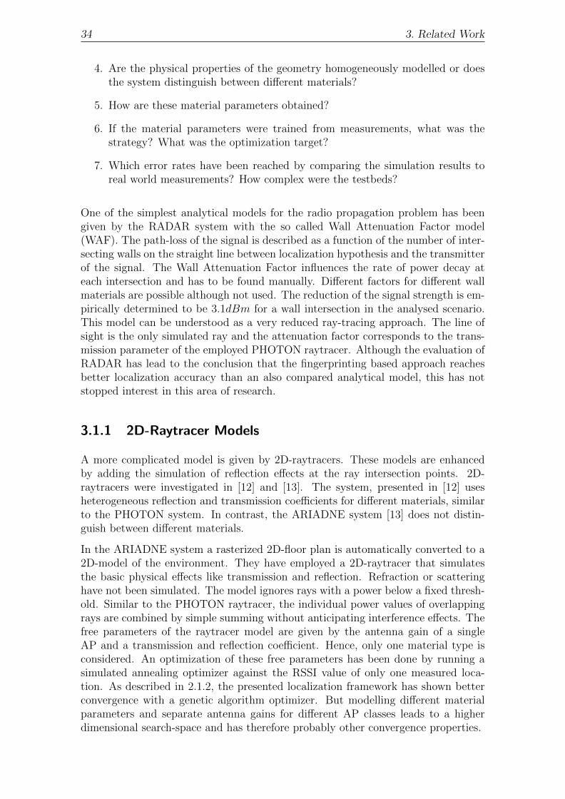
34 3. Related Work
4. Are the physical properties of the geometry homogeneously modelled or doesthe system distinguish between different materials?
5. How are these material parameters obtained?
6. If the material parameters were trained from measurements, what was thestrategy? What was the optimization target?
7. Which error rates have been reached by comparing the simulation results toreal world measurements? How complex were the testbeds?
One of the simplest analytical models for the radio propagation problem has beengiven by the RADAR system with the so called Wall Attenuation Factor model(WAF). The path-loss of the signal is described as a function of the number of inter-secting walls on the straight line between localization hypothesis and the transmitterof the signal. The Wall Attenuation Factor influences the rate of power decay ateach intersection and has to be found manually. Different factors for different wallmaterials are possible although not used. The reduction of the signal strength is em-pirically determined to be 3.1dBm for a wall intersection in the analysed scenario.This model can be understood as a very reduced ray-tracing approach. The line ofsight is the only simulated ray and the attenuation factor corresponds to the trans-mission parameter of the employed PHOTON raytracer. Although the evaluation ofRADAR has lead to the conclusion that the fingerprinting based approach reachesbetter localization accuracy than an also compared analytical model, this has notstopped interest in this area of research.
3.1.1 2D-Raytracer Models
A more complicated model is given by 2D-raytracers. These models are enhancedby adding the simulation of reflection effects at the ray intersection points. 2D-raytracers were investigated in [12] and [13]. The system, presented in [12] usesheterogeneous reflection and transmission coefficients for different materials, similarto the PHOTON system. In contrast, the ARIADNE system [13] does not distin-guish between different materials.
In the ARIADNE system a rasterized 2D-floor plan is automatically converted to a2D-model of the environment. They have employed a 2D-raytracer that simulatesthe basic physical effects like transmission and reflection. Refraction or scatteringhave not been simulated. The model ignores rays with a power below a fixed thresh-old. Similar to the PHOTON raytracer, the individual power values of overlappingrays are combined by simple summing without anticipating interference effects. Thefree parameters of the raytracer model are given by the antenna gain of a singleAP and a transmission and reflection coefficient. Hence, only one material type isconsidered. An optimization of these free parameters has been done by running asimulated annealing optimizer against the RSSI value of only one measured loca-tion. As described in 2.1.2, the presented localization framework has shown betterconvergence with a genetic algorithm optimizer. But modelling different materialparameters and separate antenna gains for different AP classes leads to a higherdimensional search-space and has therefore probably other convergence properties.
3.1. Radio Propagation 35
Figure 3.1 Schematics of the AROMA 3D-Raytracer. One the left side: ray-launching for variable antenna patterns and on the right side: material intersectionof rays.
A RPE of around 3dBm and a RPE-RMSE of 3.5dBm has been evaluated1 bycomparing the simulation results of the model against 30 measurements at validationlocations. These values are comparable to the results of the PHOTON model. Butfor using only one initial measurement during training of the free parameters, thisis a very good result.
3.1.2 3D-Raytracer Models
One of the earliest works on raytracer generated 3D radio propagation Models canbe found in [26]. The described technique was employed more recently in [8]. Thepresented raytracer simulates the physical effects of reflection and refraction. Dif-ferent antenna patterns are employed. The 3D-scene is imported from CAD outputfiles or synthesized by interpreting a 2D raster image containing a floor plan. Wallsor other anticipated solid structure from the 2D floor plan are extruded into theZ-axis with equal height. Different materials are assigned to the different parts ofthe 3D-Scene. Instead of applying some training procedure, the material parameterswere taken from literature like [30] and [20]. This is an unique approach comparedto the other presented systems.
The evaluation of the system has been conducted on a 4-room scenario of around80m2. 3 APs were placed and 3 averaged measurements at 42 locations are after-wards used for validation. A RMS-RPE of 2.28dBm is reported. The RMS-RPEdegrades to 2.83dBm, if the raytracer uses only the 2D mode. Comparing the per-formance over different sources of material parameters, the parameters in [30] haveled to the best result.
A sophisticated raytracer driven radio propagation Model is given by the AROMAframework [9]. The implemented 3D-raytracer is able to simulate the physical ef-fects of reflection, refraction and diffraction. The diffraction model is based on
1The reported value of 0.65dBm MSE has been corrected to 3.5dBm to be comparable to theother systems. Restoring the correct values was possible since a known number of 30 locationswere used.

36 3. Related Work
the Uniform Theory of Diffraction (UTD). AROMA is the only presented systemthat models the human body shadow. Detailed antenna modelling is also possible.The different properties of the antenna model that can be configured are given bytransmitting power, frequency, maximum gain and radiation pattern. Figure 3.1 il-lustrates these model assumptions. Configuration values for isotropic and half-wavedipole antenna patterns are predefined. The input for the scene geometry can begiven either in Blender or Google SketchUp format. Different material parametersare assigned to objects of the scene. It is unclear how the material parameters are de-rived, but the system exposes a preconfigured database for commonly used buildingcomponents. The simulation of the human body shadow relies on the UTD modelwith the basic assumption that a human body can be represented by the shape of acircular cylinder with radius 0.15m and height 2m.
As testbed for the evaluation, a 80m2 apartment room was chosen. 2 APs were placedand measurements at 11 locations were collected. At each location, 60 measurementsamples were taken and subsequently averaged. A RPE of 3.2dBm and RMS-RPEof 4dBm is reported on this environment.
Another advanced 3D-Raytracer model with a 2D fallback mode is presented inthesis of Martin Klepal [15]. The engine simulates the optical effects of reflection,refraction and diffraction. Non-isotropic radiation patterns for the antenna modelare also supported. The scene geometry is represented by a voxel space with avoxel edge size of 30cm for the 2GHz wave frequency. Multiple classes of materialsare supported by assigning them to the corresponding voxels. As in the presentedlocalization framework (i4lf), the material parameters are trained by optimizationwith Genetic Algorithms. The optimization criterion, also called the fitness value,is given by a minimization of a variance value which is also used during evaluation.The author reports that the Conjugate Gradient and Hill Simplex optimizationalgorithms have shown worse convergence behaviour with respect to the reachedoptimum. The impact of the number of rays on quality of the simulation is alsoanalysed. The author concludes that using 0.3 - 2 Mio rays leads to a good APcoverage estimation without artefacts due to undersaturated areas. This relatesnicely to the experience with the PHOTON raytracer where 0.3 Mio rays lead tousable and 2 Mio to excellent results with respect to the amount of artefacts inundersaturated areas.
An extensive performance evaluation was conducted on a single floor of 4 differentoffice style buildings. The floor area of all sites combined is around 5000m2. Thefour different materials, that are used in all scenes, are given by: light wall, heavywall, windows, floor. Special care has been taken by collecting the measurements.A wooden stick, that holds the device around 1m in front of the operator, wasused to minimize the body shadow effect. The number of measurement locationsand the corresponding number of received values that were probably averaged areunfortunately not disclosed. The RMS-RPE is reported to be between 3.5 and4.5dBm over the four scenes2 and corresponds to the PHOTON results as well.
2On page 84 of the thesis the author reports a computed mean and variance over the measure-ment deltas without applying the abs() function. This variance is a lower bound for the RMS-RPE.Therefore, the RMS-RPE is assumed to be around 0.5dBm higher.

3.2. Positioning and Tracking 37
3.2 Positioning and Tracking
The following sections will present literature for the major algorithmic approachesto the localization problem under the restriction of AP generated RSSI readings.An exception has been made for the related work about Particle Filters in 3.2.2.Their indoor localization approaches seems to derive of use-cases from the fieldof robot navigation and have therefore been historically adapted to other sensortypes. The presented radio propagation dependent localization systems use the RSSIinformation in an active way. This means, a mobile device is actively sensing forthe information. Recent research has also been conducted on the passive approachthat is given by measuring fluctuations in the radio propagation with stationarydevice. Such a method was proposed in [32] and has the advantage to drop the needfor special equipment at the mobile localization target in the form of some Wi-Fi-receiver. With exception of the presented system in [13], described in section 3.2.3,all RSSI based systems use a single device for measurements. In [13], three devicesare used synchronously.
3.2.1 Hidden Markov Models
In this section, three HMM based localization systems and their evaluation result arepresented. The focus is placed on the following model properties and environmentconfigurations that are used for the evaluation aspect:
1. What radio propagation model was employed? Are different materials param-eters distinguished if it is an analytical one?
2. How are is the PDFs of the emission probabilities p(x|s) modelled and bywhich means are they obtained from the radio propagation model?
3. How are the discrete PDFs of the transition probabilities p(s|s′) modelled?
4. What is the rasterization ratio of the environment that determines the area orvolume that is covered by a state?
5. How many predecessor states are evaluated and finally stored for backtrackingto the best state sequence sT1 ?
6. How was the radio propagation model configured for evaluation? How manymaterial parameters were used. How was the model obtained if it is an empir-ical one?
7. What is the size of the scene, and how are the LOS/NLOS conditions. Howmany APs were used?
8. What was the evaluation corpus of tracked paths and what is the reportederror.
The first HMM based pedestrian localization system, that is analysed here, is re-ported in [25]. For the radio propagation model an empirical model is used that
38 3. Related Work
is constructed by collecting indoor and outdoor measurements. Additionally to thestored RSSI information, sensor readings of the acceleration and from a compassare also available to the system. The database with the collected measurements wasinterpolated to obtain the emission probabilities p(x|s) at all states s representing2D locations on a grid. The database contains mean and variance information thatis used to model p(x|s) as Gaussian distributed. The evaluation of this probabilityfor a measurement x contains a smoothing step that is conducted by integrating overthe [−0.5dBm..0.5dBm] interval around the measured RSSI value. The transitionprobabilities p(s|s′) are modelled variably and depend on the sensor readings of theaccelerometer and the compass by using dead reckoning. All states are possible pre-decessor states leading to a computational complexity of T cdotS2 during the ViterbiDecoding. Finally it is a first order Markov model, as only the direct predecessorsinfluence the decision process.
An evaluation of the performance of the HMM localizer on synthetic data was con-ducted. The synthetic RSSI data is generated by assuming a radio propagationmodel with simple log-normal fading and combining it with white Gaussian noise of6dBm. The scene is a 2500m2 square area with full LOS conditions. Furthermore,additional synthetic noisy accelerometer and compass information was added to thesetup. The state space contains 2500 states with edge size 1mx1m. 9 APs wereevenly distributed. This environment leads to an offline LE of around 2m for a notexactly specified sequence of 105 measurements.
Additionally an evaluation on two real world scenes was conducted. The propagationmodel is obtained from previously collected measurements in both cases. Both caseshave an unknown number of APs and an unknown rasterization for the state space.The measurements of the three mentioned sensors were taken with a HTC HeroAndroid smartphone. The first scene is a Christmas market with area of around2500m2 at a time of the day where nearly no visitors lead to destructive body shadow.Due to the many small tourist shops at the market, there are high NLOS conditions.For this outdoor scene an offline averaged LE was evaluated on an unclear numberof measured signals. The second scene is a combination of an indoor and outdoorarea of around 1200m2. An offline LE of around 2m for the indoor, and 5m for theoutdoor part is determined. The combined LE on all 2300 measurements is givenby 4m.
Another HMM based localization system is presented in [27]. An analytical radiopropagation model was employed that is based on a multi material WAF model. Theemission probabilities p(x|s) are obtained from the WAF model that is enhanced byassuming that attenuation factors are modelled as Gaussians. The noise at thereceiver side is also modelled as a Gaussian. Both PDFs are combined to form thefinal p(x|s). As in [25], the computation of p(x|s) for an instance of the RSSI vectorx is done by integrating over the [x− 0.5dBm..x+ 0.5dBm] interval. The transitionprobabilities p(s|s′) are modelled by assuming two modes of operation. The firstmode is the movement mode which is detected by evaluating the variance from thelast 10 measurements. If the variance exceeds a preconfigured threshold, this modeis assumed to be given. The other mode can be evidently called non-movementmode. The mode configures the maximum walking speed that is used to determinethe possible transition origins s′ for the current state s. As p(s|s′) is modelled as arasterized Gaussian, the maximum walking speed is projected onto the variance. All

3.2. Positioning and Tracking 39
states are possible predecessor states although most of them will have a p(s|s′) = 0,depending on the mode controlled variance. Also, it is a HMM of first order.
The evaluation was conducted on an indoor office style scene with an area of 600m2.The WAF model is configured with 6 different material coefficients. 3 APs wereplaced to lead to NLOS conditions at the evaluation site. The 2D grid resolution of0.5mx0.5m leads to a state space with cardinality 2400. An averaged LE of around3m for this setup is reported3.
The HMM based localization system reported in [16] also uses a variant of the WAFmodel, dubbed RSSI delay profile, for simulating the radio propagation. Similar to[27] the variance of the emission probabilities p(x|s) is influenced by assumed noiseon the attenuation factors. For the transition probabilities p(s|s′), different discretetwo-dimensional PDFs are possible. All states are possible predecessor states. It isa first order Markov model.
Synthetic measurements were generated with the WAF model for an office like scenewith an area of 1200m2. The noise level of the sythetic data, given by differentvariances, should represent natural conditions. 4 APs were evenly placed to form asquare. p(s|s’) is modelled as a conic shaped two-dimensional PDF with maximumprobability at p(s|s) that is rapidly decreasing with increasing distance. On thissetup, a RMSE-LE of 5m is reported.
3.2.2 Particle Filters
Particle Filters (PF) are one of the most recent approaches to indoor localization.Historically, they originate from the field of localization for robotics. In this context,they have the typical sensor information of vehicles in the form of speed available.Two of the presented implementations can use the information of the step length andthe step heading and/or RSSI readings for pedestrian navigation. The techniquesto process this additional information source in the PF approach seems to originatein the research of robot navigation.
Four implementations will be presented by focusing on the following properties:
1. What is the available information source? If its a radio propagation model,what is the type of it?
2. How is the environment modelled, is it a 2D or 3D model?
3. How is the weighting of the particles defined? How is the state-conditional,the emission probability p(x|s) applied?
4. How are the transitions p(s|s′) modelled and how are they used during thesampling of new particles?
5. How is the problem of sample impoverishment handled?
6. On what scene was the evaluation conducted, how many particles were usedand what error rates were reached?
3The value is derived from the CDF plot as only a median of 2m is reported and there seem tobe a large number of outliers in range of > 8m

40 3. Related Work
A PF for pedestrians, targeted to support rescue operations, that uses only footstepsensor reading is presented in [29]. The sensor reports a step length, fused from anaccelerometer and a step heading that is derived from a compass. The environment is2D based and constrained by information from 2D indoor/outdoor floor plans. Theweighting of the particles is handled by a simple zero weight if the particle has crosseda wall and constant otherwise. The transition probabilities are derived from the stepheading and step length information and are combined with white Gaussian noise.Therefore, a directional sampling of new particles, comparable to dead reckoningconstraints, is employed. The PF was enhanced by an interesting approach to sampleimpoverishment problem. The basic idea is to track the history of the particles bystoring links between the new and the source particles. Therefore, each generationof particles is stored as well. Now, if the degradation of the current generation isdetected by a drop in the combined weight of all particles, the particles are tracedback into the older sample generations and the source particles of the currently”bad” particles are replaced by new samples. From these ”corrected” generations thesampling process is restarted.
The evaluation was conducted on an 2700m2 indoor/otdoor scene. A tablet PC,processing the information of XSens MTi motion sensor, was used as the mobiledevice. Map constraints from a detailed 2D-map were available. 2000 Particles areused. The averaged LE is given by 1.5m for the basic PF implementation and an evenbetter 1.3m for the variant that escapes sample impoverishment with backtracking
Another PF, that uses the same footstep sensor as the major information source,is presented in [31]. The system does also employ RSSI measurements but, theseare only used for the initialization of the particles. The particles are not uniformlydisplaced over the environment, they are constrained by a rough approximation ofthe probable localization area. The used radio propagation model for this step isa simple path-loss model without wall attenuation. The system has a notion ofthe 3D-space for multi-level building by connecting the individual 2D floor maps atjunction points and enriching the 2D map polygons with height information. This2.5D-map is used for rejecting trajectories that lead through impassable regions.The sample spawning is driven by transition probabilities that are modelled similarto [29]. The weighting of particles is also assumed to be zero if a wall is crossed. If itis a valid particle, the weight will be determined by height information for the 2.5Dmap and the height change that is additionally extracted from the footstep sensor.The transitions are modelled equally to [31] and derive their parameters from thestep length/heading information.
The evaluation was conducted on a three floor office style building with a total areaof 8725m2 that is comparable to the UMIC scene. A hip mounted PC processes thefootstep data of a XSens Mtx IMU sensor. Over 6 walks with a duration of 16mineach, a very accurate RMS-LE of less than 0.7m is reported.
In [28], three different nonlinear filters: Fourier density approximation, a gridbasedfilter and a PF are compared on an analytical and an empirical radio propagationmodel for 2D scenes. The former analytical model is a multi material WAF modeland the latter a manual collected RSSI database. In the analytical case, the weight-ing of a particle is derived from the output of the WAF model with noise from atwo-components Gaussian mixture with the two means of −7.5dBm and +7.5dBm.In the empirical case, the stored RSSI are interpolated and used as means for the mix-

3.2. Positioning and Tracking 41
ture model. In both cases, the transition probabilities p(s|s′) are circular bended onedimensional Gaussians with mean 2.5 and variance 0.3 representing average move-ment speed of 2.5m per sampling step. The problem of sample impoverishment onthe particles is not discussed.
An evaluation is conducted on synthetic data from the WAF model. The scene is anoffice style floor with an area of around 1200m2. The WAF model is configured withattenuation coefficients for three different materials. 6 APs are evenly distributed.The emission probabilities are used to generate measurements for one reference pathwith length 25m that visits three rooms in the scene. The reported offline LE is lessthan 0.8m.
On the empirical radio propagation model an evaluation with real measurements wasconducted. 14 APs were evenly distributed in the same scene. On the same path asabove, the reported averaged offline LE is less than 1m. In both experiments 500particles were used.
The last investigated implementation of a PF which uses RSSI readings can befound in [5]. The propagation model is an empirical one and is described in [6]. Theweighting is based on emission probabilities that are Gaussians with a variance of5dBm. The indoor environment is described in a 2D-map that is used to constrainthe movements during the particle sampling process. The transition probabilitiesare further modified in crossway zones to reflect the higher probability to turn indirection. Sample impoverishment is detected by a drop of the combined weights ofthe particles and is compensated by feeding new uniformly distributed particles intothe system.
The evaluation is conducted on a rectangular indoor office scene with an area of1600m2. An averaged LE of 1.9m is reached but the number of APs and the lengthof the path were unfortunately not further defined.
3.2.3 Nearest Neighboor based Approaches
For completeness, an overview of localization systems that ignore the sequentialnature of the tracking problem or that are simply only designed for the positioningproblem, will be given. These systems use the Mean Squared Error (MSE) as thedistance measure between the received RSSI vector and the stored RSSI values fora location. The location with the minimum MSE is selected as the most probablelocation. Therefore, the employed technique is labeled Least Mean Squared Error(LMSE) and was also derived in the background chapter 2.7.
A problem in the approach of LMSE is given by the result, that largely differentlocations can have similar MSEs. As a reaction to this problem, enhanced LMSE-based methods were developed. One of them is described in [18] as the so calledcloseness elimination scheme. Another in [17] where the locations at the top smallestMSEs are combined.
The system described in [8] evaluates a basic LMSE driven localizer that is based ona raytracer generated progation model. The raytracer is configured with differentmaterial coefficients that are taken directly from the literature. By using materialparameters from [30] the performance of the system is given by a RMS-LE of 2.28m
42 3. Related Work
for the positioning problem. The chosen scene for the experiments was a 130m2
small 3-room floor with three APs. The number of positioning attempts that wereevaluated is not documented.
Another framework, that is presented in [13], generalizes the LMSE selection crite-rion to a clustering based approach. Of the two known clustering strategies k-meansclustering and hierarchical clustering, the former is reported to lead to better results.The unknown initialization variable of the k-means strategy is given by the numberof target clusters. This number was determined empirically. Furthermore, the clus-ter history is exploited without formalizing the model to the state space model ofFigure 2.11. The basic idea is given by rejecting clusters at the time frame t if thebest clusters of t− 1 are too far away. The reported averaged LE is given by 2.8m.The contained tracking error is probably an online 2D-error with history constraints.
In [9] a simple localizer, based on the LMSE criterion, is used to test the qualitythe radio propagation model that is generated by the sophisticated 3D-Raytracerdescribed in section 3.1.2 of this chapter. The evaluation of the localization algorithmis performed by estimating the positions of 20 RSSI vectors that are collected foreach one of 11 predefined locations. No dependency between the 20 readings ofa single location is assumed. A pretty good LE of 1.61m is reported, although thesetting is only a smallish single-room scene of 80m2 with nearly no NLOS conditions.
3.3 Summary
The following observations were made during the evaluation of the presented litera-ture. There is no defined set of rules for determining the quality of radio propagationmodels or for comparing the performance of localization algorithms. Various errormeasures are in use and sometimes the evaluation is conducted on unclear environ-ment conditions. If needed, the presented errors have therefore been normalized tothe measures of this thesis, described in 2.1.3 and 2.3.2, for easier comparison. Itwould be helpful, if the research community could agree on some common set ofprinciples that should be mandatory for the evaluation of both topics. For example,it should be mandatory to report the number of used APs in an evaluation scene forRSSI based localization algorithms. That was not always the case.
4Design
This chapter introduces the different concepts that were needed for the realization ofthe localization framework. The core components, their use cases and their individ-ual relationships are presented. The various communication channels that connectthese components are described and the motivations for the individual architecturaldecisions are explained.
4.1 General Overview
The localization framework is build around a central server instance that communi-cates with different consumers for various purposes over HTTP. The different con-sumers are composed of mobile devices, browsers, GPU-nodes and fat clients. Thedifferent purposes for these communications are localization, measuring, evaluat-ing of results and distributing computational hard problems. The Server combinesfive major components for approaching the topics of this thesis. These componentsconsists of:
1. The Optimizer, the component responsible for training the radio propagationmodel through searching for optimal material parameter solutions by compar-ing raytracer results with a given set of initial measurements.
2. The Simulator distributes raytracing jobs to the available GPU-nodes andcollects the processing results. Either in the context of an Optimizer run orfor manual inspection of the radio propagation results for the different APs anddifferent material parameters in a debugging environment like the Fat Client.
3. The Localizer component represents the HMM and PF driven algorithms withthe associated environment needed for positioning and tracking of mobile de-vices. Therefore, its also used by the Evaluator for evaluating offline recordedmeasurements annotated with tracked positions.
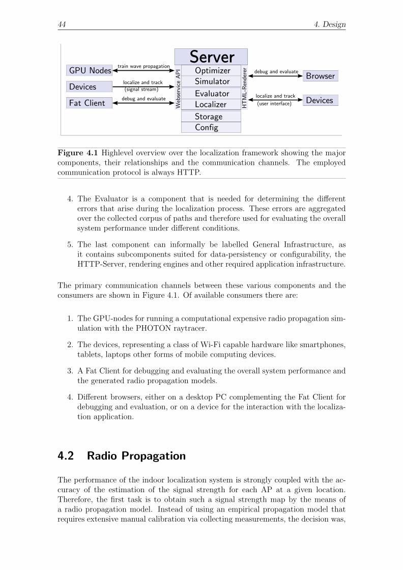
44 4. Design
Figure 4.1 Highlevel overview over the localization framework showing the majorcomponents, their relationships and the communication channels. The employedcommunication protocol is always HTTP.
4. The Evaluator is a component that is needed for determining the differenterrors that arise during the localization process. These errors are aggregatedover the collected corpus of paths and therefore used for evaluating the overallsystem performance under different conditions.
5. The last component can informally be labelled General Infrastructure, asit contains subcomponents suited for data-persistency or configurability, theHTTP-Server, rendering engines and other required application infrastructure.
The primary communication channels between these various components and theconsumers are shown in Figure 4.1. Of available consumers there are:
1. The GPU-nodes for running a computational expensive radio propagation sim-ulation with the PHOTON raytracer.
2. The devices, representing a class of Wi-Fi capable hardware like smartphones,tablets, laptops other forms of mobile computing devices.
3. A Fat Client for debugging and evaluating the overall system performance andthe generated radio propagation models.
4. Different browsers, either on a desktop PC complementing the Fat Client fordebugging and evaluation, or on a device for the interaction with the localiza-tion application.
4.2 Radio Propagation
The performance of the indoor localization system is strongly coupled with the ac-curacy of the estimation of the signal strength for each AP at a given location.Therefore, the first task is to obtain such a signal strength map by the means ofa radio propagation model. Instead of using an empirical propagation model thatrequires extensive manual calibration via collecting measurements, the decision was,
4.2. Radio Propagation 45
to use the raytracer PHOTON for generating the SSMs. Although the raytracer en-ables dynamical simulation of the radio propagation for freely placeable APs, thereare still some required prerequisites. Initially, a 3D model of the building is neededthat should preferably distinguish between materials with different physical proper-ties. For each material, the optical parameters can then be either looked-up or theyneed to be trained. In the context of this thesis, a method to train these parameterswas designed. The main motivation for these efforts was given by the circumstancesthat although material parameters were found in [30], they were not directly ap-plicable to the presented setup. It is also reasonable to assume that the propertiesof the used materials in the UMIC building differ from the ones used in other ex-periments. Furtermore, there exists no unified input format for different raytracersin general and radio propagation simulators in particular. Although probably thishurdle could be overcome by devising some adaptation scheme between differentmaterial parameter representations.
4.2.1 Model
The raytracer model consists of a Blender generated 3D-Scene with multiple meshesrepresenting the walls, doors, windows and furniture of the building. Each meshhas a defined material. For each material, there is a reflection parameter α and atransparency parameter β. Additionally, a power parameter is defined that controlsthe initial strength of the emitted signal for each AP class. APs of the same modelare grouped into such an AP class. With α and β as material parameters, theraytracer uses the following BRDF that is described in 2.1.1 for simulating theintersection between rays and materials. Refraction, diffraction and interference arenot simulated by the basic BRDF and there is no change of the direction of theray that passes through the material. For simplicity, the emission of the signal ofan AP is assumed to be isotropic. It is possible to employ more complex antennapatters that are based on spherical harmonics. But that would lead to more free,and therefore trainable, parameters instead of the chosen representation by a singlescalar power parameter for a class of APs.
The raytracer was successfully employed to simulate the radio propagation of GSM-stations in outdoor scenarios. So it is reasonable to assume, that indoor scenarios canprobably be simulated successfully as well. The raytracer is GPU-accelerated andsimulates a scene of 3000m2 over three Floors in a resolution of two megavoxels andwith 106 Rays in around 30 seconds on a NVIDIA QUADRO 6000. Therefore, theraytracer produces SSMs with a voxel size of (20cm, 20cm, 20cm). For each AP witha given position and power class such a signal strength map is generated. Duringevaluation, these maps have to be generated only once given appropriate materialparameters for the scene and power/location parameters for the APs. Hence, it isvery cheap to adapt the propagation model to a new AP configuration.
4.2.2 Parameter Estimation
For training the free parameters of the raytracer model, the implemented systemuses measurements that are collected with Wi-Fi capable devices at predefined po-sitions in the building. After this initialization phase, an evolutionary optimization
46 4. Design
process is used to find the parameter combination that minimizes the aggregatederror between the propagation simulation result and the collected measurements.
4.2.2.1 Initialization
The measurements of the signal strength for the individual APs are either collectedby using the mobile devices that should be used as localization targets later orby some special hardware like the WISPY spectrum analyzer1. The measurementsare generated by reading the device specific Wi-Fi-APIs and then transmitted overHTTP to the server instance. There, they are stored for each device separately toretain the possibility to adapt for possible device specific distortions.
Since the readings of all APs can be measured parallel at each location, the proce-dure is not time consuming. In the UMIC scenario measuring for 30 seconds at 60locations has been shown sufficient for running the parameter optimization.
4.2.2.2 Optimization
The parameter optimization is driven by a genetic algorithm on the Optimizer com-ponent. A set of free parameters constitute an organism in the context of the geneticalgorithm. The fitness of an organism is evaluated by running raytracer simulationsfor all APs over the geometry of the scene with the corresponding parameters ofthat organism. This can be a time consuming task since a representative raytracersimulation needs more than 30 seconds on a current GPU/CPU and convergence ofthe cost function is reached by evaluating at least 3000 organisms. In the analysedUMIC scenario with 22 APs, this leads to a serial processing duration of around22 days. Through exploiting the parallelizability in the cost/fitness function andthe parallel nature of the breeding phase, the duration of such an optimization runcan be reduced nearly linearly, as long as Ngpus << Npop × Naps, by employingGPU-nodes. These nodes are accessed through the Simulator component that willdistribute them accordingly.
The nodes are designed as lightweight processes that are hard wired to run thePHOTON raytracer and execute some job specific code on the results before pushingthem back to the Simulator component. The job specific code is transferred withthe job package to the node. This allows to bring new types of jobs into the systemby only updating the Server deployment. The security risk imposed by transferringthe executed result inspection code over HTTP, should be minor as the nodes pullthe jobs from a single preconfigured host. The design of the system can easilybe extended to allow automatic spawning of nodes but no real efforts have beenundertaken in that direction.
The motivation for choosing such an approach was given by the circumstances thatduring the duration of this thesis the RWTH had deployed a new GPU-Clusterconsisting of around 50 NVIDIA QUADRO 6000 nodes. By using these resourcesa full optimizing run containing 30000 simulations with a duration of 30 sec each,
1Although measurements with the WISPY were taken with the goal to derive the free raytracerparameters, the evaluation of the results were inconclusive and have thus been removed from thescope of this thesis.
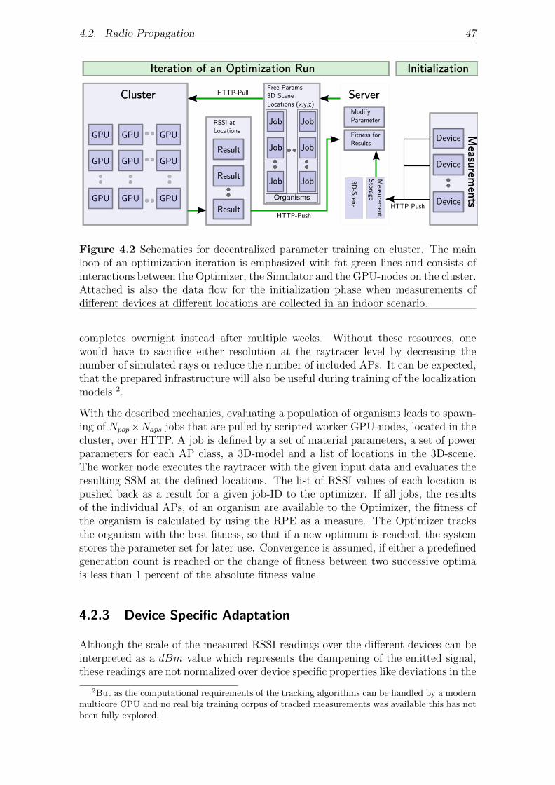
4.2. Radio Propagation 47
Figure 4.2 Schematics for decentralized parameter training on cluster. The mainloop of an optimization iteration is emphasized with fat green lines and consists ofinteractions between the Optimizer, the Simulator and the GPU-nodes on the cluster.Attached is also the data flow for the initialization phase when measurements ofdifferent devices at different locations are collected in an indoor scenario.
completes overnight instead after multiple weeks. Without these resources, onewould have to sacrifice either resolution at the raytracer level by decreasing thenumber of simulated rays or reduce the number of included APs. It can be expected,that the prepared infrastructure will also be useful during training of the localizationmodels 2.
With the described mechanics, evaluating a population of organisms leads to spawn-ing of Npop×Naps jobs that are pulled by scripted worker GPU-nodes, located in thecluster, over HTTP. A job is defined by a set of material parameters, a set of powerparameters for each AP class, a 3D-model and a list of locations in the 3D-scene.The worker node executes the raytracer with the given input data and evaluates theresulting SSM at the defined locations. The list of RSSI values of each location ispushed back as a result for a given job-ID to the optimizer. If all jobs, the resultsof the individual APs, of an organism are available to the Optimizer, the fitness ofthe organism is calculated by using the RPE as a measure. The Optimizer tracksthe organism with the best fitness, so that if a new optimum is reached, the systemstores the parameter set for later use. Convergence is assumed, if either a predefinedgeneration count is reached or the change of fitness between two successive optimais less than 1 percent of the absolute fitness value.
4.2.3 Device Specific Adaptation
Although the scale of the measured RSSI readings over the different devices can beinterpreted as a dBm value which represents the dampening of the emitted signal,these readings are not normalized over device specific properties like deviations in the
2But as the computational requirements of the tracking algorithms can be handled by a modernmulticore CPU and no real big training corpus of tracked measurements was available this has notbeen fully explored.
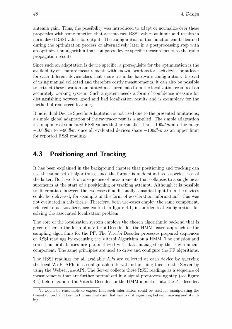
48 4. Design
antenna gain. Thus, the possibility was introduced to adapt or normalize over theseproperties with some function that accepts raw RSSI values as input and results innormalized RSSI values for output. The configuration of this function can be learnedduring the optimization process or alternatively later in a postprocessing step withan optimization algorithm that compares device specific measurements to the radiopropagation results.
Since such an adaptation is device specific, a prerequisite for the optimization is theavailability of separate measurements with known locations for each device or at leastfor each different device class that share a similar hardware configuration. Insteadof using manual collected and therefore costly measurements, it can also be possibleto extract these location annotated measurements from the localization results of anaccurately working system. Such a system needs a form of confidence measure fordistinguishing between good and bad localization results and is exemplary for themethod of reinforced learning.
If individual Device Specific Adaptation is not used due to the presented limitations,a simple global adaptation of the raytracer results is applied. The simple adaptationis a mapping of simulated RSSI values that are smaller than −100dbm into the range−100dbm to −90dbm since all evaluated devices share −100dbm as an upper limitfor reported RSSI readings.
4.3 Positioning and Tracking
It has been explained in the background chapter that positioning and tracking canuse the same set of algorithms, since the former is understood as a special case ofthe latter. Both work on a sequence of measurements that collapses to a single mea-surements at the start of a positioning or tracking attempt. Although it is possibleto differentiate between the two cases if additionally sensorial input from the devicescould be delivered, for example in the form of acceleration information3, this wasnot evaluated in this thesis. Therefore, both use-cases employ the same component,referred to as Localizer, see context in figure 4.1, in an identical configuration forsolving the associated localization problem.
The core of the localization system employs the chosen algorithmic backend that isgiven either in the form of a Viterbi Decoder for the HMM based approach or thesampling algorithms for the PF. The Viterbi Decoder processes prepared sequencesof RSSI readings by executing the Viterbi Algorithm on a HMM. The emission andtransition probabilities are parametrized with data managed by the Environmentcomponent. The same principles are used to drive and configure the PF algorithms.
The RSSI readings for all available APs are collected at each device by queryingthe local Wi-Fi-APIs in a configurable interval and pushing them to the Server byusing the Webservice-API. The Server collects these RSSI readings as a sequence ofmeasurements that are further normalized in a signal preprocessing step (see figure4.4) before fed into the Viterbi Decoder for the HMM model or into the PF decoder.
3It would be reasonable to expect that such information could be used for manipulating thetransition probabilities. In the simplest case that means distinguishing between moving and stand-ing.

4.3. Positioning and Tracking 49
Figure 4.3 Overview over the different subcomponents of the Localizer and theinteractions with the devices. The Localizer can either use a HMM, a PF or LMSEfor the core algorithmics.
Collecting measurements and evaluating them has been done asynchronously duringevaluation of the system. This means, that the measurement sequences were storedto form an evaluation corpus that was afterwards analysed. In the online trackingmode, the measurements are synchronously processed and the incrementally reportedsequence of locations is temporarily stored. The devices will pull their correspondinglocalization result by accessing the Webservice-API and visualize them in a browser.
4.3.1 Hidden Markov Model
The localization problem under the HMM approach is given by finding the most likelysequence of hidden states in a HMM for the observed sequence of measurement. Ahidden state of the HMM represents the unknown location of the device for a giventime frame. The observed emission of such a state is given by a set of RSSI readingsfor that time frame.
There are a large number of possible location sequences. If the number of measure-ments is given by T and the number of possible locations or hidden states is given byS then there are ST possible location sequences that are possible localization results.At the utilized raytracer resolution in the UMIC scene with a voxel size of 20cm,the rasterization of the 3D-space leads to 2 · 106 Voxels that represent the maximumresolution of the hidden state space . So with T = 10, this leads to around 1063 pos-sible localization results. The number of hidden states can be reduced by combiningthem into larger cubes leading to a state space with a lower resolution. This can bedone by combining a number of adjacent voxels for each dimension to a hidden statewith a larger edge size. But a brute force search for the most likely sequence of 10hidden states combined of 3 voxels with an edge size of 60cm still needs to inspect1048 candidate sequences. And that remains an intractable computational problem.
Therefore, the problem is reduced to a first-order Markov Model and the Viterbialgorithm is utilized for finding the most probable state sequence efficiently. Byusing a first-order Markov Model the Viterbi algorithm processes S states for each
50 4. Design
time frame t ∈ T . At each state st all possible predecessor states are visited. It isreasonable to limit the number of possible predecessor states to the surrounding areaof a given state. So by restricting the transitions between states to the neighbour-hood of the next two states in both horizontal directions and the next state in thevertical direction this leads to 75 predecessor states and is called a (5, 5, 3) transitionmodel. These constraints limit the number of needed computations to the tractablepolynomial complexity of 75 ·T ·S. In the UMIC scene, around 60k states with edgesize of 60cm are defined. Thus, a sequence of T = 10 measurements leads to 45 · 106
needed computations, that are processed very quickly, as the implemented decoderis able to compute 5 · 106 states per second on an Intel i7-QuadCore@3Ghz.
4.3.1.1 Parameter Estimation
The parameters of the HMM, that are evaluated by the Viterbi Decoder component,are given by the emission- and transition probabilities. These parameters are esti-mated during a training phase and are cached in the Environment component. Thedefault HMM parameter training method is given by the Baum–Welch algorithm.But for such a training, a corpus of location annotated RSSI readings is needed.That corpus needs to contain training data for all possible states, representing lo-cations in the 3D-space, so that the practicality of this approach can be excluded.Therefore, the parameters of both probabilities are acquired from other sources.
The combined SSMs over all APs is understood as a generative model for the emissionprobabilities thus these parameters can be obtained easily. But for the transitionprobabilities, no such convenient data source is at hand. The only available sourceof information, which can be exploited for modelling constraints on the movementbetween states in the 3D-space, is the 3D-model that is already used for drivingthe raytracer. At least the most critical information for modelling the transitions,the restriction which states are impassable due to blocking material, are retrievedfrom the building structure. Incorporating such knowledge is used to reject pathhypothesis that move through walls, floors or other forbidden zones.
4.3.1.2 Emission Probabilities
The model parameters for the emission probabilities p(s|x) are obtained from thestored radio propagation Models. In the UMIC scenario a hidden state is config-ured to represent the neighbourhood of 3 adjacent voxels for each dimension. Theemission probability is modelled as a multivariate Gaussian with a constant pooledcovariance matrix Σ = I. TheNaps-dimensional mean vector for p(s|x) is obtained bycalculating the arithmetic mean of the RSSI values from the 27-voxel-neighbourhoodfor each AP dimension. Although the variance of these voxel-neighbourhoods canbe calculated this does not represent any conclusive information source. The realvariance of the received RSSI values is driven by multiple effects like multipathpropagation, body shadowing and other probably location dependant noise. Noneof these effects are captured in the radio propagation model4, so the model dropsthe variance altogether. By transforming the Gaussians with Σ = I into logspace,
4Simulating the effect of multipath radio propagation on the variance could be enabled by thepossibility to dissect the raytracer results into the different recursion depths that are triggered for
4.3. Positioning and Tracking 51
Figure 4.4 Signal preprocessing recovers missing signal components (marked asgreen circles) by using information from adjacent signals and injects the neededadditional interpolated signal vectors (grey) to allow a maximum walking speed of3ms−1 under the constraints of the (5, 5, 3) model.
as described in 2.5.4, the task of the Viterbi Decoder to evaluate p(s|x) becomes asimple euclidean distance5 calculation between the stored mean vector and an inputRSSI vector.
Special attention is given to the problem of missing signals in the input vector.Although signal preprocessing mitigates this problem by interpolation of missing APcomponents in the sequence of measurement vectors (see figure 4.4), there can still bemissing AP components at the head or the tail of the sequence. If missing signals aresimply adjusted to a value of −100dbm this leads to undesirable high deltas duringthe distance calculation for the neighbouring states of the correct location. There, inthe case of a missing signal, the corresponding AP values are larger than −100dbm.With larger simulated RSSI values for such an AP at these states, the effect becomesstronger. The states near the correct location get an artificially elevated distanceand are in a sense ”pushed away”. Empirical investigations have lead to the bestresults by fully skipping the component, although assigning a distance of zero seemsto be a form of inappropriate reward for this case.
4.3.1.3 Transition Probabilities
The transition probabilities p(s|s′) are the key instruments for modelling the sequen-tial nature of the input signal. They have a discrete probability distribution that isstored in a large table containing number of states times the number of transitionsentries. The model ensures that the normalization constraints of the discrete PDFgiven by
∑s∈S p(s) = 1 and
∑s′∈S(5,5,3)
p(s|s′) = p(s) are satisfied. Furthermore, the
probability mass of p(s) is divided evenly over the three jump widths. One third isreserved for the 0-jump and the other two thirds are given to the 1- and 2-jump.
every material intersection. Overlapping signal information of different recursion depths could thenbe interpreted as a result of multipath radio propagation.
5The Viterbi Decoder can also be configured to use other distance functions. Pretty muchequivalent results in terms of errors were archived with the computational less expensive manhat-tan distance (l1-norm) restricted to the max 3 signal deltas. The restriction to the top 3 deltasanticipates the greater weight of component distances of lp-norms with p > 1

52 4. Design
Therefore, all three jumps are equal probable. If additional sensory accelerationinformation become available in a future upgrade of the system, these jumps can bedifferently weighted.
The first take on the sequential nature of the problem, is made implicitly by choosingthe (5, 5, 3)-transition-model. This can be interpreted as setting p(s|s′) = 0 for all s′
that are not included in the (5, 5, 3) neighbourhood, effectively forcing the resultingpath hypothesis to resemble a chain of locations that skips at most one state. Themodelled jump width of (0, 1, 2) is the classical approach to allow a time alignmentof the received emissions to the hidden states. In other terms, the model can adaptto different speeds of movement. Standing at a position, is by that reason modelledas a series of 0-transitions, whereas faster movement leads to series of transitionswith a higher probability of skipping states by using a jump width of 2.
By utilizing the (5, 5, 3)-model, a maximum movement speed is also introduced. Twoconsecutive signal vectors are only mapped to states that are at most 1.2m awayassuming a states represents a cube with edge size 0.6m. So in the case of gapsin the received data stream, accompanied by movements exceeding such distancethresholds, the model will not be able to compensate. Therefore, the sequence ofmeasurements is interpolated to ensure, that there are enough time frames t tocover a distance that is needed by an assumed maximum walking speed of 3ms−1
(see figure 4.4). Instead of such seemingly artificial restrictions it would alternativelybe possible to increase the maximum jump width by employing a (7, 7, 7)- or evenlarger model. But since this leads to a cubic increase in the number of allowedand therefore processable transitions for each state, this is computational expensive.Thus, the chosen (5, 5, 3)-model seems to be a good compromise between adaptivityand computational efforts.
The limitation of the maximum jump width to 1 in the vertical direction reduces thenumber of allowed transitions from 125 to 75 and is justified with the observation,that natural walking movements are primarily in the horizontal 2D-plane. Theremaining adaptivity in the vertical dimension has proven to suffice for handlingtracks containing significant parts of stairway zones6.
The next source of information that is exploited to adjust p(s|s′) for the remainingtransitions defined by the (5, 5, 3)-model is the 3D-Scene. If the 3D-cube, representedby either s or s′, intersects with a face of a 3D-object that has a material flagged asblocking, then p(s|s′) = 0. For transitions with a jump width of two, it is additionallychecked if there exists an unblocked path of at most two steps between the sourceand the destination state of the jump. If this is not the case, then p(s|s′) = 0. Thisremoves the possibility to jump over blocked cubes. See example 5 in figure 4.5.
If one of the both states is more than 2m above cubes with blocking material,then p(s|s′) = 0. This removes the possibility to fly. And the last condition forp(s|s′) = 0 is given by states, that are located above cubes containing materialflagged as impassable. This removes the possibility to walk over furniture like tablesbut only if the 3D-model exhibits detail at this level.
After applying these constraints, the probability mass for the transitions will thenbe evenly distributed over all p(s|s′) 6= 0. This results in an already reasonable
6Although the author guesses that using the elevator that is present in the UMIC scene, willprobably break this approach.
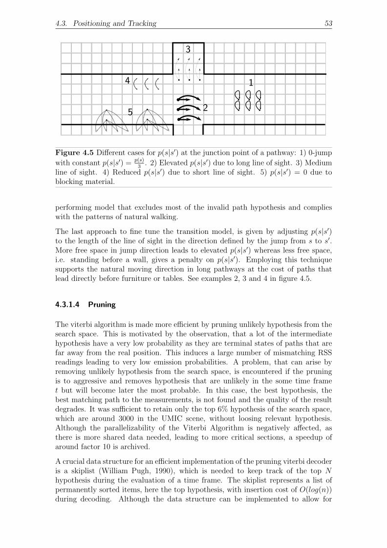
4.3. Positioning and Tracking 53
Figure 4.5 Different cases for p(s|s′) at the junction point of a pathway: 1) 0-jump
with constant p(s|s′) = p(s)3
. 2) Elevated p(s|s′) due to long line of sight. 3) Mediumline of sight. 4) Reduced p(s|s′) due to short line of sight. 5) p(s|s′) = 0 due toblocking material.
performing model that excludes most of the invalid path hypothesis and complieswith the patterns of natural walking.
The last approach to fine tune the transition model, is given by adjusting p(s|s′)to the length of the line of sight in the direction defined by the jump from s to s′.More free space in jump direction leads to elevated p(s|s′) whereas less free space,i.e. standing before a wall, gives a penalty on p(s|s′). Employing this techniquesupports the natural moving direction in long pathways at the cost of paths thatlead directly before furniture or tables. See examples 2, 3 and 4 in figure 4.5.
4.3.1.4 Pruning
The viterbi algorithm is made more efficient by pruning unlikely hypothesis from thesearch space. This is motivated by the observation, that a lot of the intermediatehypothesis have a very low probability as they are terminal states of paths that arefar away from the real position. This induces a large number of mismatching RSSreadings leading to very low emission probabilities. A problem, that can arise byremoving unlikely hypothesis from the search space, is encountered if the pruningis to aggressive and removes hypothesis that are unlikely in the some time framet but will become later the most probable. In this case, the best hypothesis, thebest matching path to the measurements, is not found and the quality of the resultdegrades. It was sufficient to retain only the top 6% hypothesis of the search space,which are around 3000 in the UMIC scene, without loosing relevant hypothesis.Although the parallelizability of the Viterbi Algorithm is negatively affected, asthere is more shared data needed, leading to more critical sections, a speedup ofaround factor 10 is archived.
A crucial data structure for an efficient implementation of the pruning viterbi decoderis a skiplist (William Pugh, 1990), which is needed to keep track of the top Nhypothesis during the evaluation of a time frame. The skiplist represents a list ofpermanently sorted items, here the top hypothesis, with insertion cost of O(log(n))during decoding. Although the data structure can be implemented to allow for
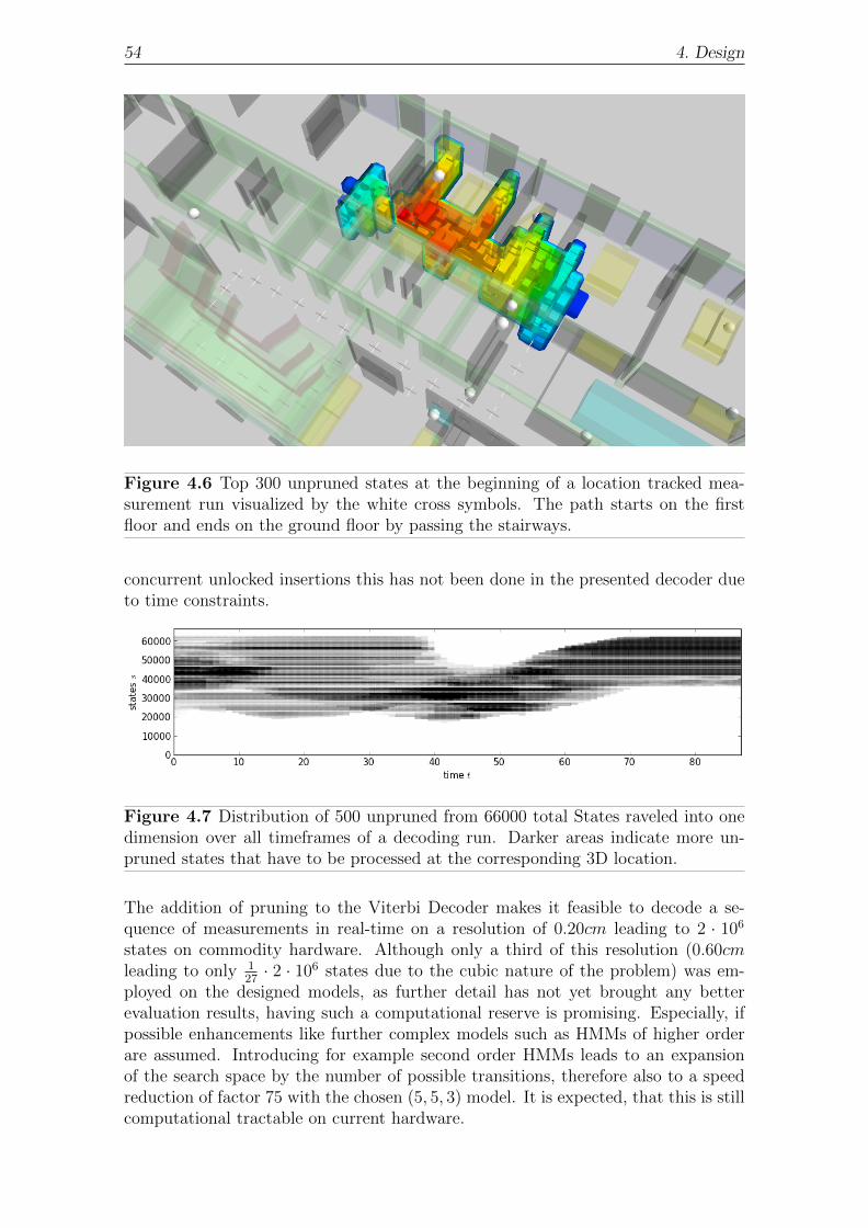
54 4. Design
Figure 4.6 Top 300 unpruned states at the beginning of a location tracked mea-surement run visualized by the white cross symbols. The path starts on the firstfloor and ends on the ground floor by passing the stairways.
concurrent unlocked insertions this has not been done in the presented decoder dueto time constraints.
Figure 4.7 Distribution of 500 unpruned from 66000 total States raveled into onedimension over all timeframes of a decoding run. Darker areas indicate more un-pruned states that have to be processed at the corresponding 3D location.
The addition of pruning to the Viterbi Decoder makes it feasible to decode a se-quence of measurements in real-time on a resolution of 0.20cm leading to 2 · 106
states on commodity hardware. Although only a third of this resolution (0.60cmleading to only 1
27· 2 · 106 states due to the cubic nature of the problem) was em-
ployed on the designed models, as further detail has not yet brought any betterevaluation results, having such a computational reserve is promising. Especially, ifpossible enhancements like further complex models such as HMMs of higher orderare assumed. Introducing for example second order HMMs leads to an expansionof the search space by the number of possible transitions, therefore also to a speedreduction of factor 75 with the chosen (5, 5, 3) model. It is expected, that this is stillcomputational tractable on current hardware.

4.3. Positioning and Tracking 55
4.3.1.5 Result Sequence
The Viterbi Decoder can return three different result sequences. The first is the bestsequence sT1 for all given measurements xT1 . This sequence represents the result ofan offline run. Furthermore, the algorithm returns the sequence containing the beststate hypothesis st for a time frame t during the viterbi decoding and representsthe results of an online run. By averaging the position over the top N locationhypothesis for a time frame t, the third result sequence sT1 is defined and called theaveraged online result. The offline sT1 has a higher probability of correctness thanthe online variants since the latter has less information to rely on, as the futuremeasurements are excluded.
4.3.2 Particle Filter
The localization problem can also be approached by modelling the states as contin-uous variables in the state space model (Figure 2.11). Such an approach is given bythe Particle Filter. As in the HMM approach, the most likely sequence of states sT1for an observed measurement sequence xT1 has to be found. But instead of searchingthis sequence by efficiently enumerating and evaluating the possible hypotheses, thesequence is generated by an iterative sampling process.
Although a basic assumption of the PF are continuous states, the system mapsthem into a discrete voxel space. Therefore, most of the data-structures from theHMM design can be reused. Voxels with 40cm edge size have shown to represent aresolution for reaching optimal results.
4.3.2.1 Emission Probabilities
The parameters of the emission probabilities p(x|s) are similar to the HMM design.p(x|s) is a Gaussian with a mean vector that is extracted from the radio propagationmodels by averaging over the RSSI values of corresponding voxel groups. The PFdoes not use the simplified logspace approach of the HMM model, and does thereforenot reduce the emission probabilities to distance based cost values. The full gaussianis evaluated and a signal variance of 5dBm has been empirically determined tolead to good results. Missing components of the input signal vector xt have beeninterpolated from neighbouring signals as described in the related HMM chapter4.3.1.2.
4.3.2.2 Transition Probabilities
The transition probability p(s|s′) is modelled as a multivariate zero-mean Gaussianwith independent components. Three dimensions of the Gaussian represent the threeaxis in free space. The variance of the horizontal components has been set to 5m andthe variance of the vertical axis to 2m. The reduced variability in the vertical axiscan be justified by the lower probability to move in that direction. Both values havebeen empirically determined by testing the PF on location annotated measurements.
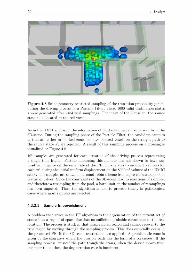
56 4. Design
Figure 4.8 Scene geometry restricted sampling of the transition probability p(s|s′)during the driving process of a Particle Filter. Here, 1000 valid destination statess were generated after 2184 trial samplings. The mean of the Gaussian, the sourcestate s′, is located at the red voxel.
As in the HMM approach, the information of blocked zones can be derived from the3D-scene. During the sampling phase of the Particle Filter, the candidate sampless, that are either in blocked zones or have blocked voxels on the straight path tothe source state s′, are rejected. A result of this sampling process on a crossing isvisualized at Figure 4.8.
105 samples are generated for each iteration of the driving process representinga single time frame. Further increasing this number has not shown to have anypositive influence on the error rate of the PF. This relates to around 1 samples foreach m3 during the initial uniform displacement on the 8900m3 volume of the UMICscene. The samples are drawn in a round-robin scheme from a pre-calculated pool ofGaussian values. Since the constraints of the 3D-scene lead to rejections of samples,and therefore a resampling from the pool, a hard limit on the number of resamplingshas been imposed. Thus, the algorithm is able to proceed timely in pathologicalcases where most samples are rejected.
4.3.2.3 Sample Impoverishment
A problem that arises in the PF algorithm is the degeneration of the current set ofstates into a region of space that has no sufficient probable connection to the reallocation. The process is stuck in that mispredicted region and cannot recover to thetrue region by moving through the sampling process. This does especially occur inthe presented PF, if the 3D-scene restrictions are applied. A problematic zone isgiven by the stairways where the possible path has the form of a corkscrew. If thesampling process ”misses” the path trough the stairs, when the device moves fromone floor to another, the degeneration case is imminent.
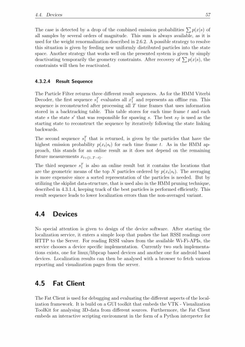
4.4. Devices 57
The case is detected by a drop of the combined emission probabilities∑p(x|s) of
all samples by several orders of magnitude. This sum is always available, as it isused for the weight renormalization described in 2.6.2. A possible strategy to resolvethis situation is given by feeding new uniformly distributed particles into the statespace. Another strategy that works well on the presented system is given by simplydeactivating temporarily the geometry constraints. After recovery of
∑p(x|s), the
constraints will then be reactivated.
4.3.2.4 Result Sequence
The Particle Filter returns three different result sequences. As for the HMM ViterbiDecoder, the first sequence sT1 evaluates all xT1 and represents an offline run. Thissequence is reconstructed after processing all T time frames that uses informationstored in a backtracking table. This table stores for each time frame t and eachstate s the state s′ that was responsible for spawing s. The best sT is used as thestarting state to reconstruct the sequence by iteratively following the state linkingbackwards.
The second sequence sT1 that is returned, is given by the particles that have thehighest emission probability p(xt|st) for each time frame t. As in the HMM ap-proach, this stands for an online result as it does not depend on the remainingfuture measurements xt+{1..T−t}.
The third sequence sT1 is also an online result but it contains the locations thatare the geometric means of the top N particles ordered by p(xt|st). The averagingis more expensive since a sorted representation of the particles is needed. But byutilizing the skiplist data-structure, that is used also in the HMM pruning technique,described in 4.3.1.4, keeping track of the best particles is performed efficiently. Thisresult sequence leads to lower localization errors than the non-averaged variant.
4.4 Devices
No special attention is given to design of the device software. After starting thelocalization service, it enters a simple loop that pushes the last RSSI readings overHTTP to the Server. For reading RSSI values from the available Wi-Fi-APIs, theservice chooses a device specific implementation. Currently two such implementa-tions exists, one for linux/libpcap based devices and another one for android baseddevices. Localization results can then be analysed with a browser to fetch variousreporting and visualization pages from the server.
4.5 Fat Client
The Fat Client is used for debugging and evaluating the different aspects of the local-ization framework. It is build on a GUI toolkit that embeds the VTK - VisualizationToolKit for analysing 3D-data from different sources. Furthermore, the Fat Clientembeds an interactive scripting environment in the form of a Python interpreter for
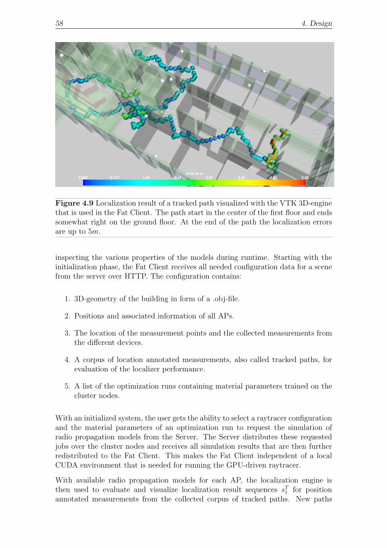
58 4. Design
Figure 4.9 Localization result of a tracked path visualized with the VTK 3D-enginethat is used in the Fat Client. The path start in the center of the first floor and endssomewhat right on the ground floor. At the end of the path the localization errorsare up to 5m.
inspecting the various properties of the models during runtime. Starting with theinitialization phase, the Fat Client receives all needed configuration data for a scenefrom the server over HTTP. The configuration contains:
1. 3D-geometry of the building in form of a .obj-file.
2. Positions and associated information of all APs.
3. The location of the measurement points and the collected measurements fromthe different devices.
4. A corpus of location annotated measurements, also called tracked paths, forevaluation of the localizer performance.
5. A list of the optimization runs containing material parameters trained on thecluster nodes.
With an initialized system, the user gets the ability to select a raytracer configurationand the material parameters of an optimization run to request the simulation ofradio propagation models from the Server. The Server distributes these requestedjobs over the cluster nodes and receives all simulation results that are then furtherredistributed to the Fat Client. This makes the Fat Client independent of a localCUDA environment that is needed for running the GPU-driven raytracer.
With available radio propagation models for each AP, the localization engine isthen used to evaluate and visualize localization result sequences sT1 for positionannotated measurements from the collected corpus of tracked paths. New paths
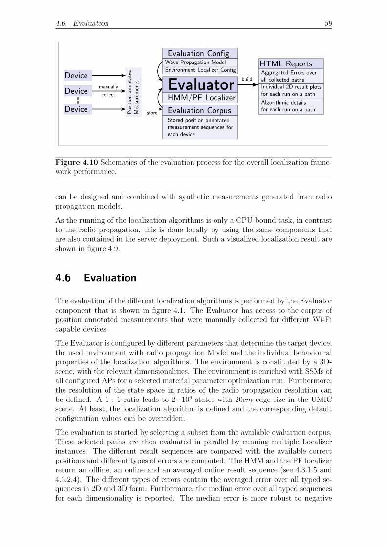
4.6. Evaluation 59
Figure 4.10 Schematics of the evaluation process for the overall localization frame-work performance.
can be designed and combined with synthetic measurements generated from radiopropagation models.
As the running of the localization algorithms is only a CPU-bound task, in contrastto the radio propagation, this is done locally by using the same components thatare also contained in the server deployment. Such a visualized localization result areshown in figure 4.9.
4.6 Evaluation
The evaluation of the different localization algorithms is performed by the Evaluatorcomponent that is shown in figure 4.1. The Evaluator has access to the corpus ofposition annotated measurements that were manually collected for different Wi-Ficapable devices.
The Evaluator is configured by different parameters that determine the target device,the used environment with radio propagation Model and the individual behaviouralproperties of the localization algorithms. The environment is constituted by a 3D-scene, with the relevant dimensionalities. The environment is enriched with SSMs ofall configured APs for a selected material parameter optimization run. Furthermore,the resolution of the state space in ratios of the radio propagation resolution canbe defined. A 1 : 1 ratio leads to 2 · 106 states with 20cm edge size in the UMICscene. At least, the localization algorithm is defined and the corresponding defaultconfiguration values can be overridden.
The evaluation is started by selecting a subset from the available evaluation corpus.These selected paths are then evaluated in parallel by running multiple Localizerinstances. The different result sequences are compared with the available correctpositions and different types of errors are computed. The HMM and the PF localizerreturn an offline, an online and an averaged online result sequence (see 4.3.1.5 and4.3.2.4). The different types of errors contain the averaged error over all typed se-quences in 2D and 3D form. Furthermore, the median error over all typed sequencesfor each dimensionality is reported. The median error is more robust to negative
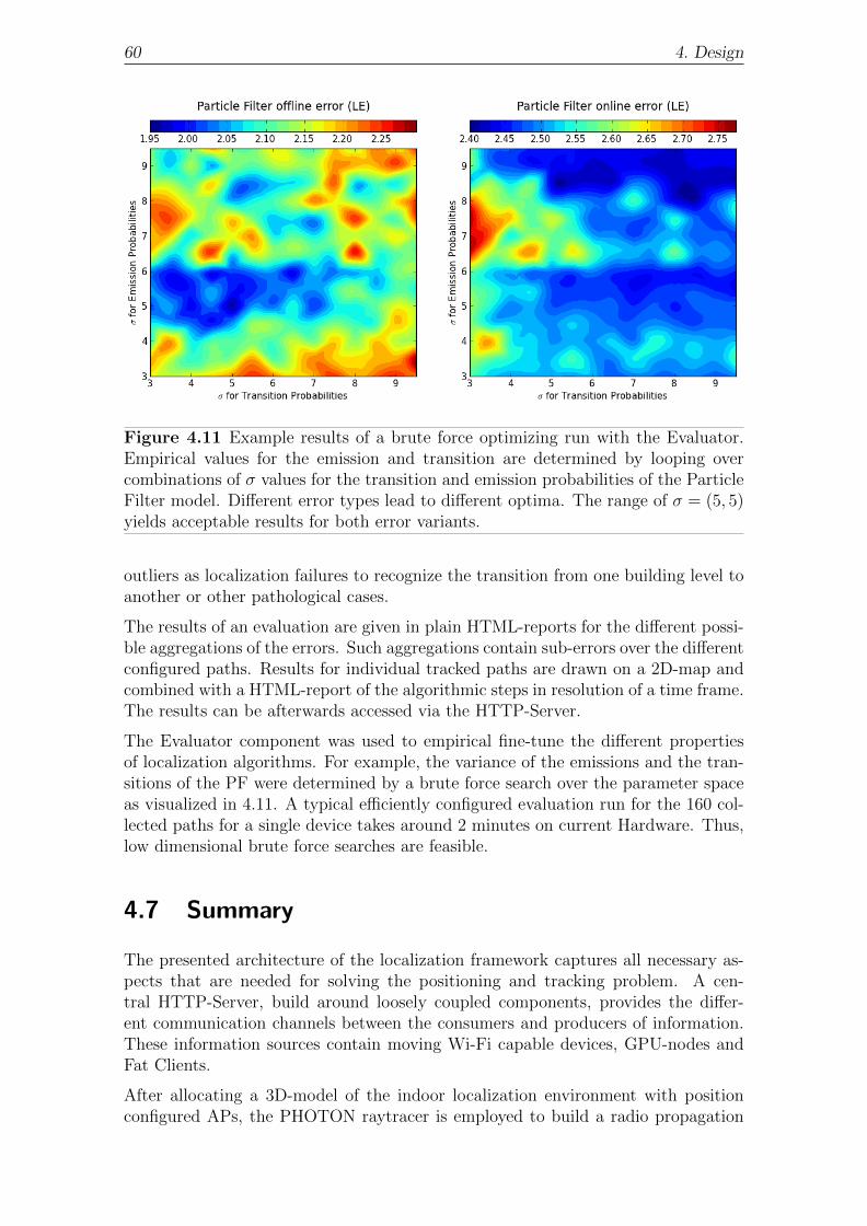
60 4. Design
Figure 4.11 Example results of a brute force optimizing run with the Evaluator.Empirical values for the emission and transition are determined by looping overcombinations of σ values for the transition and emission probabilities of the ParticleFilter model. Different error types lead to different optima. The range of σ = (5, 5)yields acceptable results for both error variants.
outliers as localization failures to recognize the transition from one building level toanother or other pathological cases.
The results of an evaluation are given in plain HTML-reports for the different possi-ble aggregations of the errors. Such aggregations contain sub-errors over the differentconfigured paths. Results for individual tracked paths are drawn on a 2D-map andcombined with a HTML-report of the algorithmic steps in resolution of a time frame.The results can be afterwards accessed via the HTTP-Server.
The Evaluator component was used to empirical fine-tune the different propertiesof localization algorithms. For example, the variance of the emissions and the tran-sitions of the PF were determined by a brute force search over the parameter spaceas visualized in 4.11. A typical efficiently configured evaluation run for the 160 col-lected paths for a single device takes around 2 minutes on current Hardware. Thus,low dimensional brute force searches are feasible.
4.7 Summary
The presented architecture of the localization framework captures all necessary as-pects that are needed for solving the positioning and tracking problem. A cen-tral HTTP-Server, build around loosely coupled components, provides the differ-ent communication channels between the consumers and producers of information.These information sources contain moving Wi-Fi capable devices, GPU-nodes andFat Clients.
After allocating a 3D-model of the indoor localization environment with positionconfigured APs, the PHOTON raytracer is employed to build a radio propagation
4.7. Summary 61
Model for the expected RSSI values. The free parameters of the model are thentrained with a genetic algorithm that is distributed over an array of GPU-nodes.
The RSSI based localization algorithms, the Hidden Markov Model and the Parti-cle Filter, are based on the same basic model assumption given by the state spacemodel of Figure 2.11. The model parameters for the emission probabilities of thetwo algorithms are derived from the trained radio propagation models. Althoughthe transition probabilities for both algorithmic approaches are modelled differently,both rely on the 3D-geometry for restricting invalid movements. Position annotatedmeasurements, for training the model parameters with the classical parameter infer-ence algorithms like the Baum-Welch algorithm in the HMM case, are not assumedto be available.
The Wi-Fi capable devices are only dumbed down information providers and haveno higher functionality.
The support infrastructure is given by the Fat Client that is used for interactivedebugging of the algorithms and associated data-streams, and finally by the Eval-uator that is utilized to measure the overall performance in terms of error rates ofthe localization framework.

62 4. Design
5Implementation
In this chapter, the implementation of the localization framework will be exam-ined under the different aspects of modern software engineering. The framework isresponsible for the training and the simulation of the PHOTON generated propa-gation models. These models are the foundation for the implemented localizationalgorithms that process the RSSI data streams of mobile devices. A GUI can beused to analyse and debug the different data streams with an interactive 3D en-gine and an evaluation engine generates HTML reports over different propagationmodel/localization algorithm settings.
The framework has been written from the scratch during the six months of this thesisand although some design decisions have been made more in an ”ad-hoc” way, it hasproven to be a valuable tool for the posed problem. The Server, the Fat Client andthe device software have been written in the Python programming language. SincePython is an interpreted languages, this makes the framework in general platformagnostic. Most of the development has been conducted under the Windows operatingsystem whereas the primary deployment of the Server is running under Linux. TheFat Client was also successfully tested under OSX.
Python is an imperative, interpreted, dynamically typed, general purpose program-ming language with a very readable syntax. All the important compound data-structures like tuples, lists, dictionaries (hash maps) and sets are first class citizensin the language and can be manipulated with powerful techniques like List/Dict/SetComprehension. Memory management is handled deterministically by a referencecounting based garbage collector. Threading support is usable for tasks that shouldhandle blocking IO, but Python byte-code will only be executed serially in the in-terpreter VM. The standard library, although not as excessive as the two behemothsJRE and CLR, covers all basic needs of modern applications. Additionally, a healthyenvironment of third party libraries, especially in the context of scientific informationprocessing and web development, satisfy all the remaining needs.
The luxuries of the Python feature set come with a cost: Python is slow. Butslowness is a relative measure. Interpreted Python is about 50 times slower than

64 5. Implementation
compiled C and still around 20 times slower than JITed Java. For most of theindividual use-cases found in the localization framework, this is fast enough. But forthe number crunching cores of the localization algorithms, the use of pure Pythoncan be excluded. Therefore, these parts of the frameworks that should be fast andmemory efficient, are implemented in Cython, a Python-to-C compiler. Cythonallows seamless integration of compiled machine code into the Python runtime andachieves significant faster execution times for computational and memory intensiveoperations.
The Python code is structured primarily with namespaces and classes. Instancesof classes are mostly used as scoping containers, higher object oriented conceptssuch as subclassing is only used sporadically in the framework. Writing idiomaticPython code, adhering to the so called Zen of Python, was a relevant design principle.Sadly, the rules of good software practice have been violated by ignoring the task ofwriting unit tests for the framework. But up till now, the implementation is ratherrepresented by laboratory than by an assembly line, so the need for them was notthat pressing either.
The third programming language that was used, is JavaScript. The output ofthe HTTP-Server includes some dynamically generated HTML pages. There, theJavaScript code is responsible for adding some interactivity to the HTML frontend.The JavaScript code is strongly JQuery driven. The following table, the output ofcloc-count1, gives an overview over the usage of the three programming languages:
Language Files Blank Comment Code
Python 26 2530 1001 8627Cython 1 472 216 1347Javascript 2 86 13 328Total 29 3088 1230 10302
5.1 Third Party Libraries
A number of open source libraries from the Python ecosystem were used in theframework. All, but Pygene, a set of genetic algorithms, are liberally licensed.Pygene uses the GPL v2, but the others are MIT like licensed. All, but Pygene,are actively maintained and backed by a strong community. But Pygene is a smalllibrary that can easily be replaced/reimplemented if that should become necessary.
The NumPy/SciPy/Matplotlib/Cython library ecosystem was the most importantfor the realization of the framework. There are no real alternatives of the samequality, so they cannot easily be replaced. The other presented libraries have ei-ther comparable alternatives or are only employed for less important use-cases asdebugging2 the data streams..
1http://cloc.sourceforge.net2Less important with respect to the final results of the thesis, but surly important for reaching
them.
5.1. Third Party Libraries 65
NumPy/SciPy/Matplotlib
The NumPy library is a major building block for the data structures of the frame-work. Numpy provides fast and efficient multi-dimensional array structures (ndar-rays) to the Python runtime. Additionally, a large number of linear algebra al-gorithms are available for the ndarrays due to linking against the BLAS/ATLASruntimes. With NumPy, tight loops of custom algorithms have to be handled withblockwise elementary operations over the ndarrays. A multitude of elementary op-erations like sum(), max(), abs(), are predefined and the method of choice if speedis crucial. But designing algorithms under that ”blockwise” philosophy leads tosomewhat awkward formulated implementations. Therefore, only the ndarray datastructures, the infrastructure for file-IO and some filters for data preprocessing/datavisualization have been used. For example, the PHOTON output is loaded directlyinto the ndarrays with a single line of NumPy.By this choices, the implementations of the localization algorithms use only thendarray data structures and implement the tight loops in Cython, as this leads tomore flexibility and readability.
The SciPy library supports NumPy by offering a large number of efficient numericalroutines working on the ndarray data structures. Especially the muti-dimensionalimage manipulation routines have proven to be very convenient during the thesis.And finally Matplotlib, a very flexible plotting library that integrates well with theNumPy data structures and provides publication quality figures. The combinationof these three libraries with Python scripting glue represents a more than adequatealternative to scientific computing environment like MATLAB.
Cython
Cython is a Python-to-C compiler that was used for implementation of the localiza-tion algorithms. If the compiler is executed on pure Python code, the gains in theform of execution speed are minimal. The real performance improvements come fromhints that are given in the form of type annotations. Tight for-loops that use onlysuch typed variables are directly translated into their C equivalents and executedindependently of the Python Virtual Machine. This leads to speed ups of multipleorders of magnitude compared to code running in the Python VM. Furthermore,strong support for the ndarray data structures is given which results in a seamlessintegration into to NumPy/SciPy/Matplotlib ecosystem. Consequently, the SciPylibrary consists of a large number of Cython implemented routines.
Another benefit of Cython comes by the flexible control over the threading behaviour.As mentioned in the introduction of this chapter, Python has no strong threadingsupport. Native OS threads are supported but the execution of the thread-specificPython byte-code is conducted serially due to a globally enforced interpreter Lock(GIL). The Cython library enables to control this locking behaviour. It allows torelease the Lock temporarily, and therefore let the Python VM continue on otherthreads. But this is only allowed if the implementation ensures not to access anyobjects from the Python runtime, during the lockless execution.This is exactly the case during the tight loops of the localization algorithms where
66 5. Implementation
accessing Python primitives like Lists or Dicts is out of the question anyway. Releas-ing the global interpreter lock makes Python based threading efficient. For example,4 instances of an algorithm can be started simultaneously from the Python VM andexecute their binary code in parallel. Even more fine grained threading control canbe reached by using the support for OpenMP instructions that are available in pureC space. By only using a slightly modified syntax for loop control, the loop becomesinstrumented by the OpenMP backend compiler support (GCC or MSVC) and willbe executed on multiple automatically spawned threads.
The localization algorithms have therefore been implemented by applying the sameprocedure: prototype the algorithm in pure Python on smallish datasets with ndar-rays. Move the Python code to Cython and make the algorithm fast by applyingtype annotations. If the algorithm is then only composed as a sequence of GIL-freeC loops over ndarrays, it can already be executed in parallel. Tuning the multi-corecapabilities even more with OpenMP has only been done for the HMM implementa-tion as the ”magic” of OpenMP imposes some constraints on the algorithm. Theseconstraints relate to sharing of variables over different scopes which would invali-date some assumptions of the Particle Filter implementation. Although this is nota surprise, as efficient parallel algorithms are often difficult to implement.
CherryPy
CherryPy is a light-weight HTTP-Server implemented in pure Python. The Servercomponent of the framework is designed as a CherryPy application. A central con-cept of a HTTP-Server, the URL-routing is defined by exposing functions of theapplication to act as URL-handlers returning some mime-type encoded string. Pro-viding a new service behind an url is therefore cheap and has made the prototyping ofthe different communication channels between the information producers/consumersan easy task. Although CherryPy acts as a standalone HTTP-Server it would makesense to run the service behind an Apache proxy server in the future.
Pygene
The Pygene library was used for the implementation of the optimization processfor the radio propagation models. It provides a set genetic algorithms that aremodelled around the concepts of population, organism and gene. Organisms are acompound data structure for genes and populations hold a number of organisms.Genes represent parameter values of an optimization and have a type correspondingto the primitive Python types like floats. Furthermore, genes can define upper andlower boundaries for their values. An organism holds a collection of genes withvalues and represents a solution in the search space of the optimizer. The searchspace is explored by crossing the genes of selected organisms from a population.This crossing leads to a new population of organisms and represents a new set ofsolutions.
It is an exotic library with respect to the GPL license and the small algorithmiccore. It would not be that hard to implement a comparable set of features, but theinner workings of genetic algorithms were of minor concern in this thesis.

5.2. Modules 67
SL4A
The Scripting Layer For Android (SL4A) framework was used for programmingthe device software. The SL4A enables the use of Python on Android devices andprovides access to the larger part of the Java-based APIs. Only the Wi-Fi APIs havebeen accessed which has resulted in around 50 lines Android specific code. It can beexpected that the distribution of SL4A based Python scripts will have deploymentissues in contrast to native Java based applications. But it would be easy to get ridof the SL4A dependency if this becomes be necessary.
Traits-UI and MayaVi
The Traits-UI and MayaVi libraries are used to drive the core of the Fat Client.Traits-UI is a Python based GUI framework with a nice balance between the needfor configurability and the ”beauty” of the results. The MayaVi library is a wrapperaround the VTK 3D visualization toolkit and provides the integration, of this excel-lent exploration tool for 3D data of different shapes, into the Traits-UI environment.Both have been shown to support a rapid prototyping style that was needed to adaptto the different ideas that have come up during the time of the thesis. The API ofthe 3D MayaVi plotting library is conveniently designed after the 2D plotting li-brary Matplotlib. This makes the mental overhead even smaller. The central Servercomponent has no dependency on the rather fat libraries.
ConfigObj
The configuation of the localization server is driven by a .ini style config format thatis processed by ConfigObj library. Its is a pure Python library with the capability tomap the string represented config parameters to primitive Python types and simplecompound structures like int lists. For this mapping a specification file, also in .inistyle format, has to be defined which represents also a good place to document thebehaviour of these values. This is comparable to define a XML-Schema for somecustom XML configuration dialect but with readability included.
JQuery
The JavaScript that is executed in the browsers of the mobile devices and on somedebugging terminals is driven by the JQuery framework. Adding dynamic elementsto the HTML pages, for example the interactive recording of location annotatedRSSI readings, has not required much efforts due to convenient API of the library.JQuery has a memory footprint of 25kb which should not pose any problems forconsumer connection conditions.
5.2 Modules
In this section, the different major components of the framework are described. Theused data structure are focused and interesting algorithmic aspects highlighted.
68 5. Implementation
5.2.1 Server
The Server component implements the core of the localization framework and isimplemented as a CherryPy application. The Server can be started from the Pythonpackage lws by pointing to a configuration file:
>> python -m lws.cli path_to_config.ini
After loading the config and initializing the HTTP-subsystem, the Server listensfor commands from the clients. If such commands arrive over the HTTP channelthey will be dispatched by the Server to the responsible subsystem. For debuggingpurposes most subsystems will be code-reloaded before processing the command.This has made developing the system very efficient.
Simulator
The Simulator is a subsystem of the Server and is responsible for coordinating theconstruction of radio propagation models. It is a singleton and drives a priorityqueue from the Python standard library. The queue contains Job() instances thatrepresent a set of material parameters and a set of .obj (Wavefront Format) files. Theconsumers of the jobs are the GPU-nodes whereas the producers of the Jobs are eitherthe Optimizer or the Fat Client. The Optimizer pushes jobs into the queue during thetraining process, and the Fat Client uses the Simulator for retrieving full propagationmodels that should analysed. The raytracer voxel arrays are compressed transmittedfrom the GPU-nodes over the Simulator to the consumers as they contain about10mb raw data that can be reduced by a factor of 3.
The priority aspect of the queue is useful for serving ”high priority” requests fromthe Fat Client before processing the next thousands of Optimizer started trainingjobs. Furthermore, it is more efficient for the Optimizer to combine all jobs for asingle genetic organism, N jobs for the evaluation of the material parameters over NAPs, in one priority slot since this leads to more efficient cluster usage.
Optimizer
The Optimizer is responsible for the training of the radio propagation models withan optimization algorithm and it employs the PyGene library for this task. It isinitialized via type checked HTTP-GET parameters over the Server component.Such a parameter set is defined in table 6.3. Additionally to the optimizer parametersa restart of older optimization runs can be enforced. This restart is implementedby deserializing the last population of the old optimization run and using it in thecurrent run. Additionally some new randomized organisms can be injected.
After the initialization phase, the core loop of the optimization run is started threaded.In the core loop, the evolutionary process is simulated by executing successive genera-tions of populations with the PyGene API. The complex part of the implementation,the custom logic for the raytracer training is implemented in the fitness() functionof a RadioPropConverger() class that is derived from a pygene.Organism(). Thefitness function is called from the PyGene framework for each organism instance of
5.2. Modules 69
a population. In this function, a Job() for each AP is queued in the Simulator andconfigured with the free parameter values obtained from gene values of the organisminstance.
The different free parameters of the model have to be declared in the genome
class variable of the RadioPropConverger(). Each element of the genome is anamed subclass of pygene.Gene(), for example in the Optimizer implementationthe MaterialGene(pygene.FloatGene) gene class is used.
If all submitted jobs are returned, the fitness of organism can be computed whichleads to progress in the population evaluation. If all organisms are fitness-evaluated,the Optimizer can decide to stop the process. This is either decided by a hard limitonto the number of allowed generations of if the difference between the quality oftwo populations becomes to small.
The individual fitness() results with the corresponding free parameters are storedand the full convergence process can be visualized with the Plotter. The output ofsuch a visualization can be seen in figure A.10.
Plotter/Evaluator
A smaller component that is only implemented at the module level, is the Plotter. Itsmain responsibility, which can be derived from the name, is the output of differentgraphics that are used to understand the localization results of the framework. It isaccessed by the Evaluator and the Server component. Whereas the Evaluator usesthe Plotter to produce plots of the evaluated localization results (see figure A.9)or other special details of the algorithms, the Server only retrieves these plots anddelivers them to the clients. The plotter uses primarily the presented Matplotliblibrary and a generic 2D drawing engine, the Python Image Library (PIL). Since thedifferent produced plots share only minor properties, the Plotter consists only of alist of functions instead of being implemented at the class level.
The Evaluator is implemented as a Python class that it responsible to evaluate theerror rates and other properties of the localization results. The instantiation of anEvaluator class is configured by a set of initialization parameters that describe thesetup of the environment and the configuration of the chosen localization algorithm.The instance can then be instrumented to analyze a part of the evaluation corpusby calling the evalAll(pathid2runids) method. The pathid2runids represents thechosen subset of the corpus and is a mapping from pathids to lists of sample runs.The chosen samples of the corpus are evaluated in parallel by using the convenientconcurrent package from the Python standard library. Since all algorithms are ex-ecuted in GIL-free C-space, the Evaluator is able to exploit multiple cores efficiently.
After computing the localization results for the chosen samples, the different variantsof the error rates are determined and stored in path-separated XML files for laterinspection.
Renderer
The last subsystem of the Server is the Renderer that is used for generating HTMLpages for the various web-browser based user interfaces. It consists only of a col-
70 5. Implementation
lection of functions that are used to generate the HTML code with Python stringprocessing capabilities. Further development on the framework will probably inducethe need for a higher level templating engine.
5.2.2 Localization Algorithms
Each localization algorithms in the presented framework is implemented as a Pythonclass derived from the Localizer() class. The Localizer() class is responsible forhandling the general interactions with the framework, whereas the subclasses imple-ment algorithmic specific code that has a low computational footprint. The imple-mentation of the computational expensive parts is relayed to the Cython languagefor each of the three algorithms.
Environment
The information about the scene specific details needed for the application of thelocalization algorithms is stored in the Environment() class which is therefore avail-able as a private member to the Localizer() derived implementations. The Envi-
ronment() class is initialized by a list of AP definitions which will lead to loadingthe corresponding stored PHOTON output files. The 3D voxel data of PHOTONis stored in .raw files which compose of a simple concatenation of float32 values,representing RSSI values, that are loaded into a 3D ndarray with NumPy-nativefunctions.
Furthermore, the scene geometry, represented by a .obj file, will also be loaded bythe Evaluator. An initialized Environment hold thus the two primary datastructuresthat are used for deriving the location conditional probabilities. The scene geometrytriangle mesh is used for generating the ndarrays for the transition probabilities.And the PHOTON output is used for computing the ndarrays for the emissionprobabilities.
HMM
The HMM based algorithm is implemented in the HMMLocalizer() Python classin conjunction with the ViterbiDecoder() Cython class. On initialization, theHMMLocalizer() loads the cached or refreshes the needed emission probabilities bydelegating the PHOTON data stored at the Environment() to the Cython func-tion buildStatesWithEmissionProbs(). The returned ndarray emission_probs
is stored at classlevel.The ndarray transition_probs for the transition probabilities is also generated inthis step. At first, the triangle mesh of the scene is voxelized by Cython acceleratedfunctions. On the voxelized representation of the geometry, the transition probabil-ities can be efficiently computed by the Cython function buildTransitionProbs.
The ViterbiDecoder() class is initialized with both ndarrays for the probabilitiesand can be used from the HMMLocalizer() for the decoding of a sequence of RSSImeasurements. The basic flow of the input in form of RSSI reading is given by the
5.2. Modules 71
call chain:HMMLocalizer().evaluateMeasurements(ms)→ self.decoder.decode(ms). Dur-ing the first call, the high level representation of the measurements that are instancesof the Measurements() class is interpolated to adjust the number of RSSI readingsto the constraints of the employed (5, 5, 3) transition model. This has to be donesince the coverable distance between two succesive RSSI vectors would be limitedto jump over two voxels. Afterwards, the measurements are additionally convertedinto an efficient indexable ndarray.
The decoding process in decode(), implements the Viterbi Algorithm described insection 2.5.2 with the designed pruning technique described in section 4.3.1.4. Tokeep track of the best hypotheses during the decoding of the RSSI values for a time-frame, the SkipList [19] datastructure is employed. This datastructure represents apermanently sorted list with efficient insertions of new members.
After decoding the unpruned state space, which is essentially composed of multipletight loops over the measurements ndarray and the ndarray of the probabilities, threePython lists representing the localization results for the online, averaged online andoffline variant are returned.
For the offline variant of the resulting sequence, the backtracking ndarray back_track
is employed which links each location hypothesis to its predecessor hypothesis. Thisndarray dominates the memory consumption of the algorithm due to its T ×S com-plexity, if T is the number of timeframes and S the number of locations. Therefore,the ndarray stores only int8 values, which represent the link by its transition in-dex which is of the range 0..75 for the (5, 5, 3) transition model. If the transitionmodel would be of higher complexity, and exceed 256 jump possibilities, the memoryconsumption would be doubled as an int16 address space becomes necessary.
Particle Filter
The Python side of the PF algorithm, in the form of the PFLocalizer() class,is very similar to the described HMMLocalizer(). Contrary to the HMM case, notransition probabilities are generated from the scene geometry. Only the voxelizedrepresentation of the geometry is constructed that is later used for rejecting particlesthat interfere with that structure. The other difference is given by the missing inter-polation step of the RSSI readings, as constraints like the (5, 5, 3) HMM transitionmodel are not given.
The PFLocalizer() prepares a pool of values for a three dimension Gaussian thatare used in a round-robin scheme during the particle spawning or sampling process.This spawning is a part of the simulation of the modelled stochastic process which isimplemented as the Cython sibling class ParticleFilter(). This class is initializedwith and ndarray containg emission probabilities, the sampling pool and the vox-elized representation of blocked zones. All three ndarrays are used during decodingthe RSSI sequence.
To efficiently keep track of the top N hypothesized locations for a single timeframe,the SkipList datastructure is used similar as in the HMM case. The top N hypothe-sized locations of a time frame are used for calculating the averaged online predictionof a location.
72 5. Implementation
Like the HMMLocalizer(), the PFLocalizer() decoder returns three lists of posi-tions for the offline, online and averaged online result variant.
LMSE
The most simple algorithm, is the LMSE based approach which is implemented inthe LMSELocalizer() class and the corresponding LMSE() Cython decoder class.The Python side computes only the ndarray for the emission probabilities for thevoxelized RSSI values for each AP. This ndarray initializes the LMSE() class that isafterwards instrumented via its decode(ms) function to evaluate the measurementsequence of the input signals.
To efficiently keep track of the top N solutions for the nearest neighbour distancecomputations that are executed over the total localization space, the already in theHMM and the PF employed SkipList structure is used. The top N solutions can beunderstood as a simple clustering of the best locations and has for example in theARIADNE [13] system been enhanced to a k-means clustering model.
5.2.3 Fat Client
The Fat client is the primary debugging tool for the behaviour of the radio prop-agation models and the algorithmic progress of the localization algorithms. It isbuild around the Traits-UI GUI toolkit that conveniently embeds the MayaVi 3Dengine for scalar data visualization of the localization space. The location relatedscalar data has to be given in the form of ndarrays that are already used all over theimplementation of the framework. Most transformations of the algorithm specificndarrays to a MayaVi compatible structure is done by the native functionality ofthe NumPy/SciPy libraries. If the solution could only be awkwardly implementedwith NumPy block operations, Cython functions have been implemented for betterreadability and flexibility.
The GUI needs access to the described Server infrastructure that is defined by itsHTTP address. It uses the Server for initialization to a specific 3D geometry andthe corresponding AP placement. Furthermore, it can investigate the training cor-pus for the radio propagation models and the evalution corpus for the localizationalgorithms. The PHOTON generated RSSI predictions can be visualized with theMayaVi engine after beeing processed by the GPU-nodes and subsequently deliveredby the Server. Due to the GPU-driven nature of the PHOTON raytracer, this designchoice makes sense as no special hardware and CUDA driver setup is needed on theclient side.
As mentioned, the evaluation corpus for the localization algorithms are also fetchedfrom the Server over HTTP and can be used to investigate the results of the al-gorithms. The algorithms are executed locally as the Fat Client has access to thecode of the corresponding modules from the Server infrastructure. The different Lo-calizer() classes can be instantiated with Environment() conditions that can bemanipulated from the GUI. The algorithmic progress from timeframe to timeframeof the top N location hypotheses can be visualized for the HMM, PF and LMSEimplementations. This is very helpful to find weaknesses in algorithmic properties.
5.3. Summary 73
Another convenient implementation detail of the Fat Client is given by the embed-ded Python interpreter which can be used to analyse most datastructures of theframework interactively. Formulating questions over this scripting interface is veryefficient from a developer point of view.
5.3 Summary
In this chapter, a cursory overview of the chosen programming paradigms and someof the implementation details have been presented. As can be observed, the devel-oper of the system, the author of the thesis was satisfied with the implementationresults that have been reached under the constraints of a six-month thesis. Thechoice of Python and Cython as development platform has lead to an efficientlyprototyped localization framework that employs fast algorithms with a low memoryfootprint. The chosen open source libraries, especially the NumPy/SciPy/Matplotlibecosystem, have shown to be of very high quality and can therefore be recommendedas well.

74 5. Implementation
6Evaluation
This chapter is dedicated to the evaluation of the presented localization framework.Special attention is given to the description of the setting and the environment con-ditions of the experiments as this was often only briefly reported in the investigatedliterature1.
After describing the experimental setup, the results for the training process of theradio propagation models are analysed. A focus is placed on the behaviour of thetraining process under different levels of 3D geometry granularity. An additionalexperiment for the radio propagation context is conducted by evaluating the abilityof the models to generalize over multiple devices. The generated models and the cor-responding observations are subsequently used for the evaluation of the localizationalgorithms that were designed and implemented.
It will be reported how the three algorithms, the LMSE, the HMM and the PF, per-form on a selected fully trained propagation model. In the first step, the algorithmsare compared on synthetic data obtained from the propagation model under differ-ent noise levels. The differences between the results of the individual algorithmsare explained by their underlying algorithmic properties. The use of synthetic datamakes this task easier.
Using the results of the radio propagation evaluation and the experiences from theanalysis on synthetic data enables a thorough investigation of the framework perfor-mance on real world conditions. Location annotated RSSI readings for a distance ofabout 8000m were manually collected for eight different track configurations of vari-ous complexity. This evaluation corpus is used to estimate the localization errors ofthe three algorithms over differently trained radio propagation models. Furthermore,the effect of the devised Device Adaptation scheme described in 4.2.3, is analysedand interpreted.
1Although it should be emphasized, that the investigated literature was mostly available in theform of journal papers which have surely made compromises due to page count constraints.

76 6. Evaluation
6.1 Radio Propagation Model
The evaluation of the framework starts with a detailed explanation of the environ-ment that is used for the experiments. The introduction of the setup starts bydescribing the different properties of the manually created 3D geometry that is uti-lized to drive the PHOTON raytracer. Afterwards, the placement of the differentAP groups and the resulting coverage conditions is analysed. In the next step, thecomposition of the training corpus that drives the optimization process is presented.A relevant number of measurements over 100 locations in the UMIC scene weretaken with four different Android devices. These measurements will represent thelargest part of the training corpus that is employed in the evaluation.
After the introductory part, it will be seen how plausible the trained propagationmodels adapt to the true nature of the environment by using the optimization crite-rion, the RPE, as a measure2. An experiment that investigates the training processover measurements of different devices and another one that tries to understandhow important the granularity of the 3D geometry is, will finalize this part of theevaluation.
6.1.1 Scene and Setup
The evaluated localization scenario is located in the UMIC Building3 of the RWTHAachen. It is a four level building with a rectangular floor-area of around 900m2.The first three floors were modelled in Blender leading to a volume of around 8100m3,as the height of a level is around 3m. It is composed of ”reduced to functionality”office architecture and was erected in the year 2009.
6.1.1.1 3D-Model and Materials
The 3D-model consists of 11 different object classes given in the form of triangularmeshes. The class of an object is defined by the assigned material. The choice ofthe materials was made by reasoning about their importance of their impact on theradio propagation. Probably the most important ones are the Concrete and theLightWalls class of objects. 2D-Maps of the building at the resolution of these twomaterials were available and are used as a base for these two classes of objects in the3D-model. Further modelled detail is given by doors with the three material classesIronDoor, normal Doors and GlassDoor. The limits of the building are modelledwith the two materials Fascade and GlassWindow. Additional furniture details arecaptured by the materials Cupboard and Table. Also included for completeness is themetal based railing of the stairs and hardware components that are located next tosome of the APs or components that exhibit a massive structure, like the hardwarearray of the server room.
2This can lead to a serious overfitting of the model, but since the training corpus had only asize of 100 locations it has been concluded that they are to valuable to sacrifice some of them toallow the better cross-validation technique.
3Google Maps reference: http://g.co/maps/q3mp6
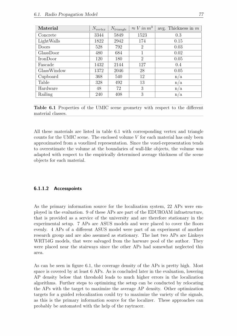
6.1. Radio Propagation Model 77
Material Nvertex Ntriangle ≈ V in m3 avg. Thickness in m
Concrete 3344 5849 1523 0.3LightWalls 1822 2942 174 0.15Doors 528 792 2 0.03GlassDoor 480 684 1 0.02IronDoor 120 180 2 0.05Fascade 1432 2144 127 0.4GlassWindow 1372 2046 28 0.05Cupboard 368 540 12 n/aTable 328 492 13 n/aHardware 48 72 3 n/aRailing 240 408 3 n/a
Table 6.1 Properties of the UMIC scene geometry with respect to the differentmaterial classes.
All these materials are listed in table 6.1 with corresponding vertex and trianglecounts for the UMIC scene. The enclosed volume V for each material has only beenapproximated from a voxelized representation. Since the voxel-representation tendsto overestimate the volume at the boundaries of wall-like objects, the volume wasadapted with respect to the empirically determined average thickness of the sceneobjects for each material.
6.1.1.2 Accesspoints
As the primary information source for the localization system, 22 APs were em-ployed in the evaluation. 9 of these APs are part of the EDUROAM infrastructure,that is provided as a service of the university and are therefore stationary in theexperimental setup. 7 APs are ASUS models and were placed to cover the floorsevenly. 4 APs of a different ASUS model were part of an experiment of anotherresearch group and are also assumed as stationary. The last two APs are LinksysWRT54G models, that were salvaged from the harware pool of the author. Theywere placed near the stairways since the other APs had somewhat neglected thisarea.
As can be seen in figure 6.1, the coverage density of the APs is pretty high. Mostspace is covered by at least 6 APs. As is concluded later in the evaluation, loweringAP density below that threshold leads to much higher errors in the localizationalgorithms. Further steps to optimizing the setup can be conducted by relocatingthe APs with the target to maximize the average AP density. Other optimizationtargets for a guided relocalization could try to maximize the variety of the signals,as this is the primary information source for the localizer. These approaches canprobably be automated with the help of the raytracer.
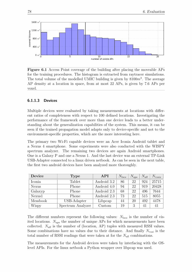
78 6. Evaluation
Figure 6.1 Access Point coverage of the building after placing the moveable APsfor the training procedures. The histogram is extracted from raytracer simulations.The total volume of the modelled UMIC building is given by 8100m3. The averageAP density at a location in space, from at most 22 APs, is given by 7.6 APs pervoxel.
6.1.1.3 Devices
Multiple devices were evaluated by taking measurements at locations with differ-ent ratios of completeness with respect to 100 defined locations. Investigating theperformance of the framework over more than one device leads to a better under-standing about the generalization capabilities of the system. This means, it can beseen if the trained propagation model adapts only to device-specific and not to theenvironment-specific properties, which are the more interesting here.
The primary two Wi-Fi capable devices were an Acer Iconia Android tablet anda Nexus 4 smartphone. Some experiments were also conducted with the WISPYspectrum analyzer. The remaining two devices are again Android smartphones.One is a Galaxy P and one a Nexus 1. And the last device was an external TP-LinkUSB-Adapter connected to a linux driven netbook. As can be seen in the next table,the first two android devices have been analyzed more thoroughly.
Device Type API Nlocs Naps Nall Nrssis
Iconia Tablet Android 3.2 86 22 924 25715Nexus Phone Android 4.0 94 22 919 20428Galaxyp Phone Android 2.3 68 22 496 7644Nexus1 Phone Android 2.3 73 22 515 8055Messbook USB-Adapter Libpcap 44 20 492 4478Wispy Spectrum Analyzer Custom 19 3 41 41
The different numbers represent the following values: Nlocs is the number of vis-ited locations. Naps the number of unique APs for which measurements have beencollected. Nall is the number of (location, AP) tuples with measured RSSI values.Some combinations have no values due to their distance. And finally Nrssi is thetotal number of RSSI readings that were taken at for the Nall combinations.
The measurements for the Android devices were taken by interfacing with the OS-level APIs. For the linux netbook a Python wrapper over libpcap was used.
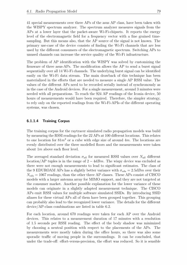
6.1. Radio Propagation Model 79
41 special measurements over three APs of the asus AP class, have been taken withthe WISPY spectrum analyzer. The spectrum analyzer measures signals from theAPs at a lower layer that the packet-aware Wi-Fi-chipsets. It reports the energylevel of the electromagnetic field for a frequency vector with a fine grained time-sampling. But this means also, that the AP source of the signal is not known. Theprimary use-case of the device consists of finding the Wi-Fi channels that are lessused by the different consumers of the electromagnetic spectrum. Switching APs tounused channels can increase the service quality of the Wi-Fi infrastructure.
The problem of AP identification with the WISPY was solved by customizing thefirmware of three asus-APs. The modification allows the AP to send a burst signalsequentially over all 14 Wi-Fi channels. The underlying burst signal can be identifiedeasily on the Wi-Fi data stream. The main drawback of this technique has beenmaterialized in the efforts that are needed to measure a single AP RSSI value. Thevalues of the different APs need to be recorded serially instead of synchronously asin the case of the Android devices. For a single measurement, around 3 minutes wereneeded with all preparations. To reach the 924 AP readings of the Iconia device, 50hours of measurements would have been required. Therefore, the simpler strategy,to rely only on the reported readings from the Wi-Fi-APIs of the different operatingsystems, was chosen.
6.1.1.4 Training Corpus
The training corpus for the raytracer simulated radio propagation models was buildby measuring the RSSI readings for the 22 APs at 100 different locations. This relatesto one location for 81m3 or a cube with edge size of around 4m. The locations areevenly distributed over the three modelled floors and the measurements were takenabout 1m above each floor level.
The averaged standard deviation σall for measured RSSI values over Nall differentlocation/AP tuples is in the range of 2− 4dBm. The wispy device was excluded asthere were not enough measurements to lead to significant estimates. The class ofthe 9 EDUROAM APs has a slightly better variance with σedu = 2.5dBm over theirNedu = 1067 readings, than the other three AP classes. These APs consist of CISCOmodels with a larger antenna array for MIMO support, and they are not targeted atthe consumer market. Another possible explanation for the lower variance of thesemodels can originate in a slightly adapted measurement technique. The CISCOAPs emit RSSI values for multiple software simulated SSIDs. By introducing SSIDaliases for these virtual APs all of them have been grouped together. This groupingcan probably also lead to the recognized lower variance. The details for the differentdevice/AP-class combinations are listed in table 6.2.
For each location, around 670 readings were taken for each AP over the Androiddevices. This relates to a measurement duration of 17 minutes with a resolutionof 1.5 seconds per RSSI reading. The effect of the body shadow was minimizedby choosing a neutral position with respect to the placements of the APs. Themeasurements were mostly taken during the office hours, so there was also somesporadic traffic of moving people in the surroundings. It can be concluded, thatunder the trade-off: effort-versus-precision, the effort was reduced. So it is sensible
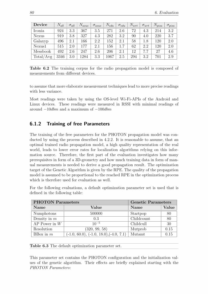
80 6. Evaluation
Device Nall σall Nasus σasus Nedu σedu Nwrt σwrt Npisa σpisa
Iconia 924 3.3 367 3.5 271 2.6 72 4.3 214 3.2Nexus 919 3.8 327 4.3 282 3.2 90 4.0 220 3.7Galaxyp 496 2.1 166 2.2 152 2.1 58 1.8 120 2.0Nexus1 515 2.0 177 2.1 156 1.7 62 2.2 120 2.0Messbook 492 2.6 247 2.6 206 2.1 12 7.7 27 4.6Total/Avg 3346 3.0 1284 3.3 1067 2.5 294 3.2 701 2.9
Table 6.2 The training corpus for the radio propagation model is composed ofmeasurements from different devices.
to assume that more elaborate measurement techniques lead to more precise readingswith less variance.
Most readings were taken by using the OS-level Wi-Fi-APIs of the Android andLinux devices. These readings were measured in RSSI with minimal readings ofaround −10dbm and a maximum of −100dbm
6.1.2 Training of free Parameters
The training of the free parameters for the PHOTON propagation model was con-ducted by using the process described in 4.2.2. It is reasonable to assume, that anoptimal trained radio propagation model, a high quality representation of the realworld, leads to lower error rates for localization algorithms relying on this infor-mation source. Therefore, the first part of the evaluation investigates how manyprerequisites in form of a 3D-geometry and how much training data in form of man-ual measurements is needed to derive a good propagation result. The optimizationtarget of the Genetic Algorithm is given by the RPE. The quality of the propagationmodel is assumed to be proportional to the reached RPE in the optimization processwhich is therefore used for evaluation as well.
For the following evaluations, a default optimization parameter set is used that isdefined in the following table:
PHOTON Parameters Genetic ParametersName Value Name Value
Numphotons 500000 Startpop 80Density in m 0.3 Childcount 80AP Power in W 10−5 Childcull 30Resolution (320, 99, 58) Mutprob 0.15BBox in m (-1.0, 60.0), (-1.0, 18.0),(-4.0, 7.1) Mutamt 0.15
Table 6.3 The default optimization parameter set.
This parameter set contains the PHOTON configuration and the initialization val-ues of the genetic algorithm. Their effects are briefly explained starting with thePHOTON Parameters :
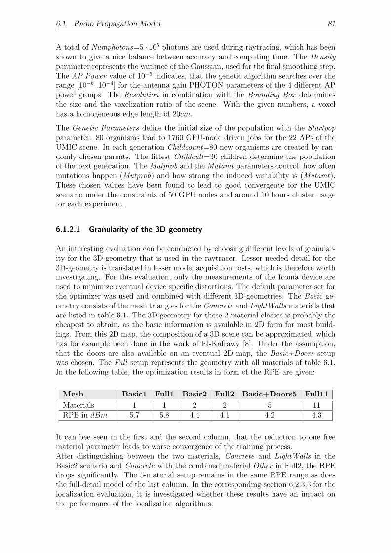
6.1. Radio Propagation Model 81
A total of Numphotons=5 · 105 photons are used during raytracing, which has beenshown to give a nice balance between accuracy and computing time. The Densityparameter represents the variance of the Gaussian, used for the final smoothing step.The AP Power value of 10−5 indicates, that the genetic algorithm searches over therange [10−6..10−4] for the antenna gain PHOTON parameters of the 4 different APpower groups. The Resolution in combination with the Bounding Box determinesthe size and the voxelization ratio of the scene. With the given numbers, a voxelhas a homogeneous edge length of 20cm.
The Genetic Parameters define the initial size of the population with the Startpopparameter. 80 organisms lead to 1760 GPU-node driven jobs for the 22 APs of theUMIC scene. In each generation Childcount=80 new organisms are created by ran-domly chosen parents. The fittest Childcull=30 children determine the populationof the next generation. The Mutprob and the Mutamt parameters control, how oftenmutations happen (Mutprob) and how strong the induced variability is (Mutamt).These chosen values have been found to lead to good convergence for the UMICscenario under the constraints of 50 GPU nodes and around 10 hours cluster usagefor each experiment.
6.1.2.1 Granularity of the 3D geometry
An interesting evaluation can be conducted by choosing different levels of granular-ity for the 3D-geometry that is used in the raytracer. Lesser needed detail for the3D-geometry is translated in lesser model acquisition costs, which is therefore worthinvestigating. For this evaluation, only the measurements of the Iconia device areused to minimize eventual device specific distortions. The default parameter set forthe optimizer was used and combined with different 3D-geometries. The Basic ge-ometry consists of the mesh triangles for the Concrete and LightWalls materials thatare listed in table 6.1. The 3D geometry for these 2 material classes is probably thecheapest to obtain, as the basic information is available in 2D form for most build-ings. From this 2D map, the composition of a 3D scene can be approximated, whichhas for example been done in the work of El-Kafrawy [8]. Under the assumption,that the doors are also available on an eventual 2D map, the Basic+Doors setupwas chosen. The Full setup represents the geometry with all materials of table 6.1.In the following table, the optimization results in form of the RPE are given:
Mesh Basic1 Full1 Basic2 Full2 Basic+Doors5 Full11
Materials 1 1 2 2 5 11RPE in dBm 5.7 5.8 4.4 4.1 4.2 4.3
It can bee seen in the first and the second column, that the reduction to one freematerial parameter leads to worse convergence of the training process.After distinguishing between the two materials, Concrete and LightWalls in theBasic2 scenario and Concrete with the combined material Other in Full2, the RPEdrops significantly. The 5-material setup remains in the same RPE range as doesthe full-detail model of the last column. In the corresponding section 6.2.3.3 for thelocalization evaluation, it is investigated whether these results have an impact onthe performance of the localization algorithms.

82 6. Evaluation
6.1.2.2 Multiple Devices
In this experimental setup, three propagation models were trained by using measure-ments from the training corpus for different device combinations. The first propa-gation model was only trained on the Iconia tablet, the second model includes themeasurements of the Nexus smartphone and the last model uses measurements fromall four Android based devices. The reached RPE under the parameter optimizationare reported in the following table:
Device Iconia Iconia/Nexus Iconia/Nexus/Galaxyp/Nexus1
RPE in dBm 4.3 3.6 5.0
Although the combination of the four devices in the last column leads to a highRPE of around 5dBm, the theory, that more employed devices lead to worse prop-agation models is contradicted by the first two results. The combination of theIconia/Nexus measurements exhibits an even better converging optimization pro-cess than the Iconia-only case. It also shows satisfying results with respect to theevaluation of the localization algorithms. Such an evaluation is conducted for theIconia/Nexus model in the following section 6.2.3.2.
6.2 Localization
This section presents the performance evaluation of the three presented localizationalgorithms. The HMM and the PF are compared with respect to the baseline giventhrough the LMSE approach. After describing the properties of the evaluation siteand the different evaluated localization paths, the algorithms are initially tested onsynthetic data. This will allow to compare them under idealized conditions withrespect to errors originating in the radio propagation model. The required artificialsequences of RSSI vectors are therefore obtained from the SSMs generated by thePHOTON raytracer.
After the synthetic evaluation, the performance of the localization framework on realworld data will be analysed. Experiments with two different devices classes, a tabletand a smartphone, were conducted. The real world experiments are composed ofmultiple localizations paths, that were manually tracked and annotated to establishthe evaluation corpus for the localization problem.
6.2.1 Scene and Setup
The evaluation was conducted in the UMIC building, described in 6.1.1, over twoandroid devices, the Iconia tablet and a Galaxy Nexus smartphone. Eight pathsthat lead through the building with various degrees of complexities were defined andsubsequently used for taking the measurement streams. Each path has a forwardand a backward variant which effectively doubles the number of tracked paths tosixteen. The tables 6.4 and 6.5 show the different properties of the defined paths indetail.
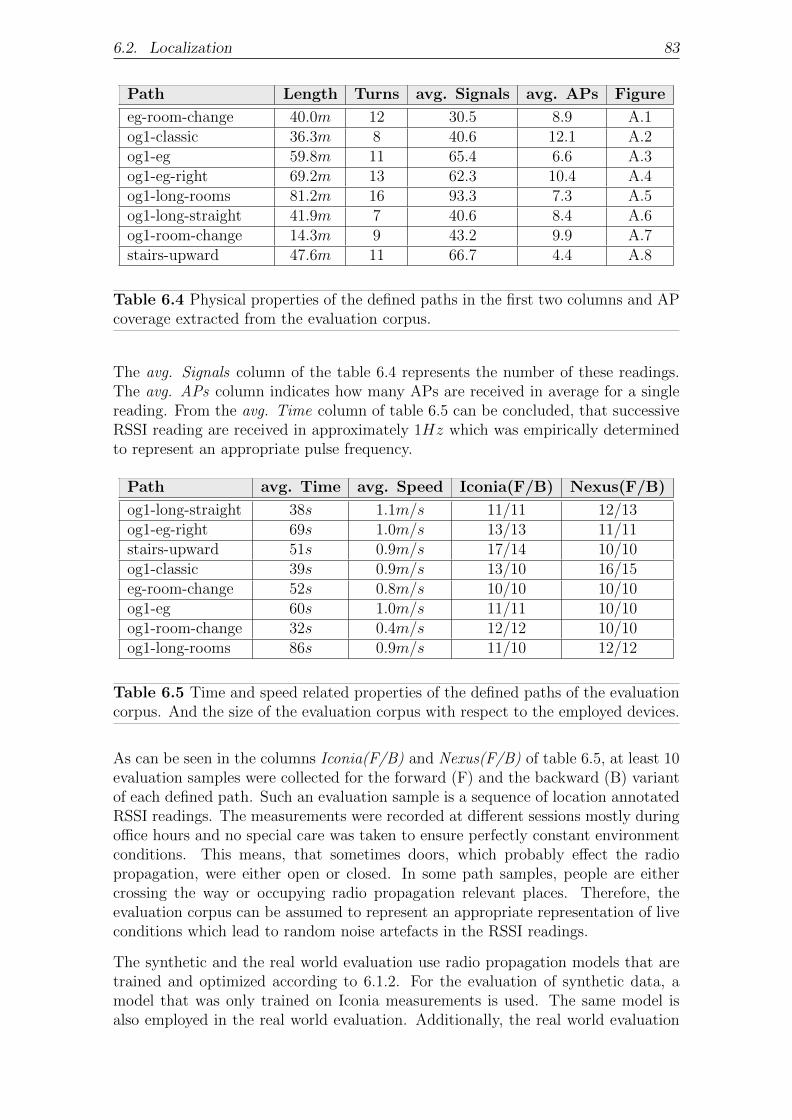
6.2. Localization 83
Path Length Turns avg. Signals avg. APs Figure
eg-room-change 40.0m 12 30.5 8.9 A.1og1-classic 36.3m 8 40.6 12.1 A.2og1-eg 59.8m 11 65.4 6.6 A.3og1-eg-right 69.2m 13 62.3 10.4 A.4og1-long-rooms 81.2m 16 93.3 7.3 A.5og1-long-straight 41.9m 7 40.6 8.4 A.6og1-room-change 14.3m 9 43.2 9.9 A.7stairs-upward 47.6m 11 66.7 4.4 A.8
Table 6.4 Physical properties of the defined paths in the first two columns and APcoverage extracted from the evaluation corpus.
The avg. Signals column of the table 6.4 represents the number of these readings.The avg. APs column indicates how many APs are received in average for a singlereading. From the avg. Time column of table 6.5 can be concluded, that successiveRSSI reading are received in approximately 1Hz which was empirically determinedto represent an appropriate pulse frequency.
Path avg. Time avg. Speed Iconia(F/B) Nexus(F/B)
og1-long-straight 38s 1.1m/s 11/11 12/13og1-eg-right 69s 1.0m/s 13/13 11/11stairs-upward 51s 0.9m/s 17/14 10/10og1-classic 39s 0.9m/s 13/10 16/15eg-room-change 52s 0.8m/s 10/10 10/10og1-eg 60s 1.0m/s 11/11 10/10og1-room-change 32s 0.4m/s 12/12 10/10og1-long-rooms 86s 0.9m/s 11/10 12/12
Table 6.5 Time and speed related properties of the defined paths of the evaluationcorpus. And the size of the evaluation corpus with respect to the employed devices.
As can be seen in the columns Iconia(F/B) and Nexus(F/B) of table 6.5, at least 10evaluation samples were collected for the forward (F) and the backward (B) variantof each defined path. Such an evaluation sample is a sequence of location annotatedRSSI readings. The measurements were recorded at different sessions mostly duringoffice hours and no special care was taken to ensure perfectly constant environmentconditions. This means, that sometimes doors, which probably effect the radiopropagation, were either open or closed. In some path samples, people are eithercrossing the way or occupying radio propagation relevant places. Therefore, theevaluation corpus can be assumed to represent an appropriate representation of liveconditions which lead to random noise artefacts in the RSSI readings.
The synthetic and the real world evaluation use radio propagation models that aretrained and optimized according to 6.1.2. For the evaluation of synthetic data, amodel that was only trained on Iconia measurements is used. The same model isalso employed in the real world evaluation. Additionally, the real world evaluation
84 6. Evaluation
uses an Iconia/Nexus trained model to investigate whether the localization systemgeneralizes over multiple devices. The optimization result of these two models isreported in 6.1.2.2. Furthermore, the distinction between the different devices isonly made during the real world evaluation.
Offline/Online Results
For both evaluation setups, the three algorithms are compared. The PF and theHMM approach return Offline and Online results. Both adapt to RSSI informationcontained in the history due to their algorithmic nature. The offline result is thepredicted sequence of locations under the knowledge of the full history. The onlineresult is the predicted sequence of locations under the knowledge of the limitedhistory up to a time frame. The latter represents the result that is available for auser of a localization service who expects to be informed about his current locations,and not about the way he came.
Therefore, it is reasonable to distinguish between the online and the offline resultand it can be expected, that the offline variant outperforms the online result due toits larger knowledge pool. The LMSE does not use the history of the RSSI values,therefore it reports only an online result.
The online error of the PF and the HMM is given in an additional averaged form.This form is defined by using the mean location over the top 50 candidate hypothesisof a time frame t instead of choosing the best hypothesized location.
6.2.2 Synthetic Measurements
In this section, the performance of the three localization algorithms is evaluated onsynthetically generated RSSI sequences used to simulate readings of a mobile devicewith different noise conditions. For each of the 16 path variants 20 samples weregenerated therefore leading to 320 evaluated path samples. From the lengths ofthe paths given in table 6.4 can be derived that around 8000m of covered distanceare evaluated. The average movement speed is assumed to be 1m/s reflecting theproperties of the real world measurements that are concluded from table 6.5. Forevery 0.75s, an RSSI vector is generated that represents the target frequency of theRSSI pushing android devices4.
The synthetic measurements were generated by using the RSSI values of a trainedradio propagation model as the means of Gaussians with a variable noise σ. Fromthese Gaussians the measurements are sampled for 0dBm ≤ σ ≤ 18dBm with astep size of 0.5dBm. The results for the algorithmic variants under online andoffline conditions, for a localization space with 40cm voxel size, can be obtainedfrom figure 6.2 and table 6.6.
It can be seen, that the LMSE based algorithm leads to incompetitive error ratesover all noise conditions with respect to the HMM and the PF approach. This wasexpected since it does not use the valuable information contained in the measurement
4Although the target frequency was not completely reached in the real world measurements dueto network latency over the HTTP communication channel.

6.2. Localization 85
Figure 6.2 Online and offline 2D localization errors over 36 noise steps. The HMMoutperforms the PF during the online and offline mode. The averaged online resultleads to lower errors for both algorithms.
history. Interestingly, it is even slower than the PF, since all states of the locationspace have to be visited at each time frame. And this is costly for a high resolutionstate space.
The HMM algorithm leads to the lowest error rates over all noise conditions. Evenboth online errors are lower than the PF offline error. This comes by the costs ofincreased computational complexity by the factor 10 and an increase in memoryconsumption of around factor 100. It can be concluded that the HMM approachreaches lower error rates: By conducting an exhaustive search over the hypothesesthe HMM approach is guaranteed to find the optimal solution, whereas the PFapproach is not to able to generate this solution by sampling.
Furthermore, both algorithms show the behaviour that the averaged variant of theonline error leads to a better prediction of the hidden location sequence but areoutperformed by the offline error in both cases. An interpretation of this result is,that valuable information is distributed over either the particles or the unprunedstates of the HMM. The backtracked solutions in the offline mode can make senseof this information whereas during the online mode it can only partially be accessedby the averaging process.
Additionally, it can be observed from the variance plot in figure 6.2, that the PF,compared to the HMM, shows an elevated decrease in accuracy under increasingnoise at the interval 8dBm < σ < 14dBm. By investigating the individual resultsequences it was observed that at these noise levels the effect of sample impoverish-ment (see 4.3.2.3) becomes significant and seems not to be handled optimal. It isonly countered with random re-sampling which induces a new noise component andtherefore leads to a degraded result. A better way to handle the decay of the set ofparticles in the PF algorithm is proposed in the work of Widyawan [29]. The basicidea is to conserve the particle history, manipulate it by using information from the
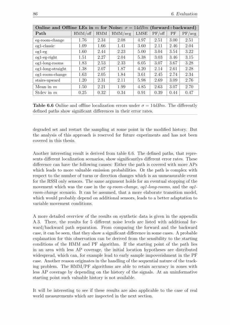
86 6. Evaluation
Online and Offline LEs in m for Noise: σ = 14dBm (forward+backward)Path HMM/off HMM HMM/avg LMSE PF/off PF PF/avg
eg-room-change 1.76 2.34 2.08 4.97 2.51 3.00 2.51og1-classic 1.09 1.66 1.41 3.60 2.11 2.46 2.04og1-eg 1.60 2.44 2.23 5.00 3.04 3.54 3.22og1-eg-right 1.51 2.27 2.04 5.38 3.03 3.46 3.15og1-long-rooms 1.83 2.53 2.33 6.05 3.07 3.67 3.28og1-long-straight 1.38 2.07 1.87 4.20 2.14 2.61 2.28og1-room-change 1.63 2.05 1.84 3.61 2.45 2.74 2.34stairs-upward 1.20 2.31 2.11 5.98 2.69 3.09 2.76
Mean in m 1.50 2.21 1.99 4.85 2.63 3.07 2.70Stdev in m 0.25 0.32 0.34 0.91 0.39 0.44 0.47
Table 6.6 Online and offline localization errors under σ = 14dBm. The differentlydefined paths show significant differences in their error rates.
degraded set and restart the sampling at some point in the modified history. Butthe analysis of this approach is reserved for future experiments and has not beencovered in this thesis.
Another interesting result is derived from table 6.6. The defined paths, that repre-sents different localization scenarios, show significantlys different error rates. Thesedifference can have the following causes: Either the path is covered with more APswhich leads to more valuable emission probabilities. Or the path is complex withrespect to the number of turns or direction changes which is an unmeasurable eventfor the RSSI only sensors. The same argument holds for an eventual stopping of themovement which was the case in the eg-room-change, og1-long-rooms, and the og1-room-change scenario. It can be assumed, that a more elaborate transition model,which would probably depend on additional sensors, leads to a better adaptation tovariable movement conditions.
A more detailed overview of the results on synthetic data is given in the appendixA.3. There, the results for 5 different noise levels are listed with additional for-ward/backward path separation. From comparing the forward and the backwardcase, it can be seen, that they show a significant difference in some cases. A probableexplanation for this observation can be derived from the sensibility to the startingconditions of the HMM and PF algorithm. If the starting point of the path liesin an area with less AP coverage, the initial location hypotheses are distributedwidespread, which can, for example lead to early sample impoverishment in the PFcase. Another reason originates in the handling of the sequential nature of the track-ing problem. The HMM/PF algorithms are able to retain accuracy in zones withless AP coverage by depending on the history of the signals. At an uninformativestarting point such valuable history is not available.
It will be interesting to see if these results are also applicable to the case of realworld measurements which are inspected in the next section.
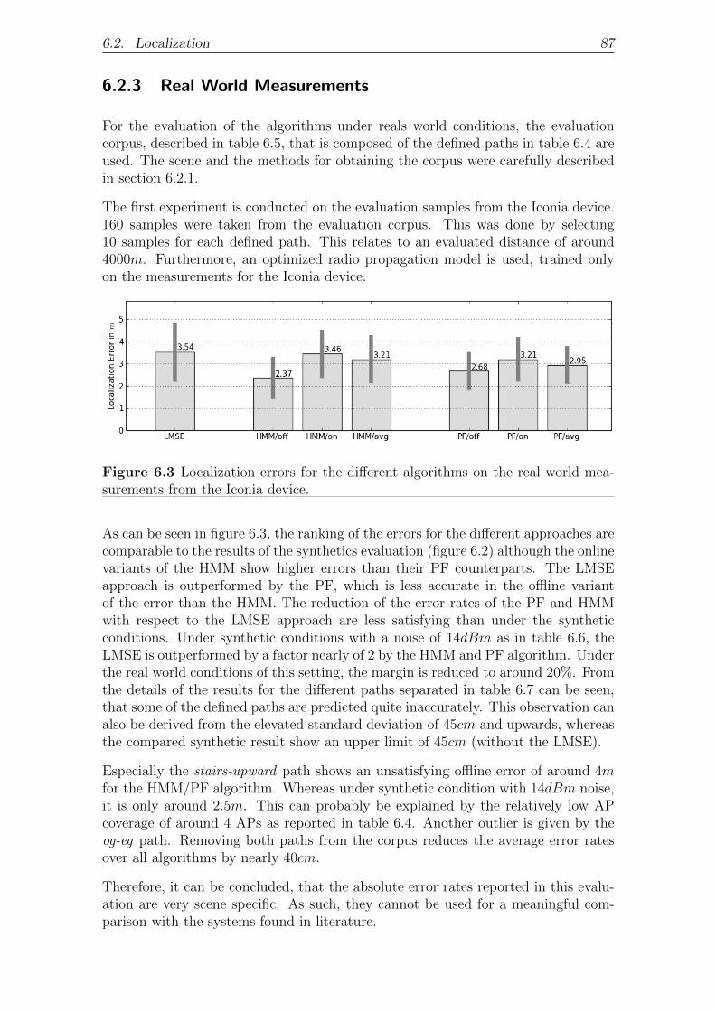
6.2. Localization 87
6.2.3 Real World Measurements
For the evaluation of the algorithms under reals world conditions, the evaluationcorpus, described in table 6.5, that is composed of the defined paths in table 6.4 areused. The scene and the methods for obtaining the corpus were carefully describedin section 6.2.1.
The first experiment is conducted on the evaluation samples from the Iconia device.160 samples were taken from the evaluation corpus. This was done by selecting10 samples for each defined path. This relates to an evaluated distance of around4000m. Furthermore, an optimized radio propagation model is used, trained onlyon the measurements for the Iconia device.
Figure 6.3 Localization errors for the different algorithms on the real world mea-surements from the Iconia device.
As can be seen in figure 6.3, the ranking of the errors for the different approaches arecomparable to the results of the synthetics evaluation (figure 6.2) although the onlinevariants of the HMM show higher errors than their PF counterparts. The LMSEapproach is outperformed by the PF, which is less accurate in the offline variantof the error than the HMM. The reduction of the error rates of the PF and HMMwith respect to the LMSE approach are less satisfying than under the syntheticconditions. Under synthetic conditions with a noise of 14dBm as in table 6.6, theLMSE is outperformed by a factor nearly of 2 by the HMM and PF algorithm. Underthe real world conditions of this setting, the margin is reduced to around 20%. Fromthe details of the results for the different paths separated in table 6.7 can be seen,that some of the defined paths are predicted quite inaccurately. This observation canalso be derived from the elevated standard deviation of 45cm and upwards, whereasthe compared synthetic result show an upper limit of 45cm (without the LMSE).
Especially the stairs-upward path shows an unsatisfying offline error of around 4mfor the HMM/PF algorithm. Whereas under synthetic condition with 14dBm noise,it is only around 2.5m. This can probably be explained by the relatively low APcoverage of around 4 APs as reported in table 6.4. Another outlier is given by theog-eg path. Removing both paths from the corpus reduces the average error ratesover all algorithms by nearly 40cm.
Therefore, it can be concluded, that the absolute error rates reported in this evalu-ation are very scene specific. As such, they cannot be used for a meaningful com-parison with the systems found in literature.

88 6. Evaluation
Path HMM/off HMM HMM/avg LMSE PF/off PF PF/avg
eg-room-change 1.71 2.91 2.66 2.31 1.56 2.25 2.16og1-classic 1.46 2.85 2.60 2.65 2.13 2.59 2.46og1-eg 3.04 4.35 4.13 4.21 3.18 3.89 3.59og1-eg-right 1.85 2.83 2.52 3.19 2.62 2.90 2.56og1-long-rooms 2.02 3.54 3.40 3.86 2.82 3.08 2.93og1-long-straight 2.94 4.00 3.84 3.32 2.62 3.28 3.32og1-room-change 2.58 2.66 2.36 2.59 2.54 2.71 2.54
stairs-upward 3.17 3.49 3.22 5.82 3.50 4.35 3.58stairs-upward-r 3.55 5.53 5.08 6.48 4.42 5.59 4.43
Mean in m 2.37 3.46 3.21 3.54 2.68 3.21 2.95Stdev in m 0.68 0.87 0.87 1.17 0.69 0.85 0.66
Table 6.7 Detailed errors for the different paths from the evaluation corpus. Theaggregation of the results can be seen in figure 6.3. The stairs-upward-r path, thatis addionally shown in the forward/backward variant, is a drastic negative outlier,probably due to complex nature of the stairway scene and the suboptimal placementsof APs.
Figure 6.4 Localization error over all algorithms for the Iconia device after apply-ing the Device Adaptation technique. The error rates for the PF and the LMSEalgorithm drop by around 20cm.
6.2.3.1 Device Adaptation
The evaluation is continued by investigating the Device Adaptation method de-scribed in the design chapter 4.2.3. This method assumes, that the reported RSSIvalues from the device are distorted with respect to some unknown function. Theconfiguration of this function can be learned from the radio propagation models iflocation annotated measurements are available for the individual model of the deviceor for the more general device class.
Such a function was trained for the previously described and evaluated Iconia setup.As the mentioned location annotated measurements, the training corpus for the radiopropagation model was used. The comparison of the results in figure 6.4 with theprevious results in figure 6.3 reveals that the procedure has a measurable effect onthe error rates. For the PF and the LMSE algorithm, the reduction is about 20cm.The error rates of the HMM approach are reduced by about 40cm. Not surprisingly,
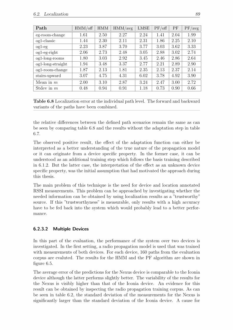
6.2. Localization 89
Path HMM/off HMM HMM/avg LMSE PF/off PF PF/avg
eg-room-change 1.61 2.50 2.27 2.24 1.41 2.04 1.99og1-classic 1.44 2.30 2.11 2.31 1.86 2.25 2.10og1-eg 2.23 3.87 3.70 3.77 3.03 3.62 3.33og1-eg-right 2.06 2.73 2.48 3.05 2.88 3.02 2.74og1-long-rooms 1.80 3.03 2.92 3.45 2.46 2.86 2.64og1-long-straight 1.94 3.48 3.37 2.77 2.21 2.89 2.90og1-room-change 1.87 2.13 1.81 2.35 2.13 2.37 2.14stairs-upward 3.07 4.75 4.31 6.02 3.78 4.92 3.90
Mean in m 2.00 3.10 2.87 3.24 2.47 3.00 2.72Stdev in m 0.48 0.94 0.91 1.18 0.73 0.90 0.66
Table 6.8 Localization error at the individual path level. The forward and backwardvariants of the paths have been combined.
the relative differences between the defined path scenarios remain the same as canbe seen by comparing table 6.8 and the results without the adaptation step in table6.7.
The observed positive result, the effect of the adaptation function can either beinterpreted as a better understanding of the true nature of the propagation modelor it can originate from a device specific property. In the former case, it can beunderstood as an additional training step which follows the basis training describedin 6.1.2. But the latter case, the interpretation of the effect as an unknown devicespecific property, was the initial assumption that had motivated the approach duringthis thesis.
The main problem of this technique is the need for device and location annotatedRSSI measurements. This problem can be approached by investigating whether theneeded information can be obtained by using localization results as a ”trustworthy”source. If this ”trustworthyness” is measurable, only results with a high accuracyhave to be fed back into the system which would probably lead to a better perfor-mance.
6.2.3.2 Multiple Devices
In this part of the evaluation, the performance of the system over two devices isinvestigated. In the first setting, a radio propagation model is used that was trainedwith measurements of both devices. For each device, 160 paths from the evaluationcorpus are evaluted. The results for the HMM and the PF algorithm are shown infigure 6.5.
The average error of the predictions for the Nexus device is comparable to the Iconiadevice although the latter performs slightly better. The variability of the results forthe Nexus is visibly higher than that of the Iconia device. An evidence for thisresult can be obtained by inspecting the radio propagation training corpus. As canbe seen in table 6.2, the standard deviation of the measurements for the Nexus issignificantly larger than the standard deviation of the Iconia device. A cause for

90 6. Evaluation
Figure 6.5 The two devices, the Iconia tablet and the Nexus smartphone, showcomparable error rates on a radio propagation model that is trained with measure-ments from both.
this behaviour can be found by remembering the device classes of both models. TheIconia is a tablet device with a ten inch display, whereas the Nexus is of the smallersmartphone device class. Due to the size of its body, a possible interpretation is,that the Iconia tablet is equipped with a larger antenna which leads to smother RSSIreadings.
Figure 6.6 Interestingly, the Nexus smartphone outperforms the Iconia tablet, withrespect to the localization accuracy, on a radio propagation model, that is onlytrained on the latter.
In the last part of the evaluation it is investigated whether the assumption holds,that the radio propagation model generalizes over the two used devices. Therefore,an experiment with both devices is conducted on a radio propagation model that isonly trained with measurements of the Iconia device. The results of the employedmodel for the Iconia were already shown in figure 6.3. Using the model also for theNexus device leads to the results of figure 6.6.
Comparing the results of both devices leads to the conclusion, that the Iconia trainedradio propagation model generalizes well for the Nexus specific localization problem.The reported error rates for the Nexus are even lower for most algorithmic combi-nations which has not been expected.
The next step of the evaluation is conducted by adding an additional Device Adap-tation step as described in the previous section 6.2.3.1. Figure 6.7 reports the resultsof this procedure.

6.2. Localization 91
Figure 6.7 The Device Adaptation shows no effect on the error rates of the Nexus.
Figure 6.8 Localization errors for radio propagation models trained on materialannotated 3D geometry of different complexities. From left to right, the geome-try becomes more complex. It can be observed that using the most complex ge-ometry of Full11 leads unexpectedly to worse results than using the less complexBasic+Doors5.
Under the Iconia trained propagation model, the Device Adaptation for the Nexusshows no significant enhancement. The results become even marginally worse. Un-der the assumption, that the Device Adaptation is a form of final training for radiopropagation model, this result makes no sense. The measurements of the Nexusdevice should have been a valuable information to adapt to the less ”familiar” prop-agation model as it has only be trained on the Iconia device.
6.2.3.3 Granularity of the 3D geometry
In the following experiment, the impact of the accuracy of the 3D geometry on thelocalization error is analysed. Six radio propagation models were trained on 3Dgeometry that represents the UMIC environment in different levels of complexity.The details of the six models are described in the former evaluation of these modelsin section 6.1.2.1.
160 path samples originating from the Iconia device were selected from the evaluationcorpus, as including the samples from the Nexus can lead to undesired device specificdistortions in the outcome of the experiment. The samples are evaluated with allthree localization algorithms which leads to results that are listed in figure 6.8.
Unexpectedly, the single material variants Basic1 and Full1 perform worse thanthe other variants. This underperformance was also visible in the reported RPE
92 6. Evaluation
of section 6.1.2.1. It can therefore be concluded, that modelling the environmentwith one material leads to an insufficient propagation model with respect to thelocalization problem. Even increasing the complexity of the scene geometry doesnot leads to improvements. On the contrary, the Full1 propagation model performsless accurate than the simpler Basic1 model.
The Basic2 propagation model performs very good with regard to its simple meshstructure. Only the concrete and light walls are employed in the 3D geometry whichis a relatively easy to obtain information about a building. The model leads tobetter error rates over all algorithms compared to the Full2 model. The Full2 canbe understood as an upgraded variant of the geometry from Basic2. They share thescene objects composed of concrete material, but the Full2 combines all remainingavailable triangles to the secondary material, whereas the Basic2 only uses the lightwalls for that. Concluding from the error rates, this seems to be a bad approach.
It is an interesting result, that the Basic+Doors5 geometry outperforms the Full11model on the HMM/PF algorithms quite significantly and leads to the overall bestresults. The additional knowledge that is included in the most complex model Full11seems not to be an exploitable information source for the raytracer under the setupof this thesis.
6.3 Summary
From the overall results presented in this chapter, it can be summarized that the de-signed framework is able to solve the localization problem with acceptable accuracyfor PHOTON driven radio propagation models. The proposed method of trainingthe free model parameters with genetic algorithms leads to material and AP spe-cific coefficients that are usable to generate RSSI estimates that diverge only about4dBm from the true reality represented by the training corpus. By further devicespecific fine tuning with the presented Device Adaptation scheme, the divergencecan be reduced to 3.5dBm.
The analysis of the performance of the three different localization algorithms hasbrought up the conclusion that the HMM approach outperforms the PF approachover most scenarios. On synthetic data, the gap between the error rates of bothalgorithms is more significant than under real world conditions. On an assumednoise level of 14dBm, the offline error of the HMM approach is given by a promising1.5m whereas the Particle Filter reaches only an offline accuracy of 2.6m. As wasexpected from its algorithmic properties, the simple LMSE approach leads not tocompetitive results on synthetic data, as it reports a localization error of around 5m.
The relations between the error rates of the algorithms shift quite significantly ifthe evaluation is conducted on real world measurements. The HMM and the Par-ticle Filter algorithm perform now very similar although the HMM shows a visibleadvantage under offline conditions. The average error rates over all defined pathsare in the range of 2− 3m for most evaluated scenarios. It was observable, that theerror rates between paths of different complexity show a high variability. Especiallythe stairway path can only be inferred with an accuracy of less than 4m. Removingthis path and another outlier shifts the offline/online error rates down to 1.5m/2.0mover the remaining six easier scenarios.
6.3. Summary 93
The proposed Device Adaptation technique shows a promising increase of accuracyfor the Iconia device but only inconclusive results for the Nexus. The localizationexperiments, that were conducted over both devices, lead to the conclusion thatthe trained propagation models are able to generalize over multiple devices. Thesystem reports similar error rates if the propagation model is trained with eitheronly measurements from the Iconia or from the combined measurements of bothdevices.
The final evaluation step, the investigation of how much granularity of the 3D geom-etry is needed for the PHOTON generated propagation models that are subsequentlyused for estimating the localization errors, lead to an interesting result. The bestperforming radio propagation variant is driven by a 3D geometry only consisting ofconcrete material, light walls and three different types of doors (iron, glass, normal).The full detail model that contains additional elements like windows and furnitureis somewhat overspecified for the PHOTON → localization algorithm pipeline. Butthis leads also to the more positive result, that sufficient detailed geometry can prob-ably be generated automatically from rasterized 2D floor maps, since both types ofwalls and the location of doors can be obtained from them in most cases.

94 6. Evaluation
7Conclusion
The motivation of this thesis, the analysis of state-of-the-art localization algorithmsbased on the prediction of Wi-Fi signal distributions has lead to the design of alocalization framework providing a combined controll of the raytracing system, thelocalization system and the evaluation tools. The implemented system was em-ployed to build a representative evaluation corpus for the localization problem and atraining corpus for the Wi-Fi prediction problem. The evaluation of the predictioncapabilities of the used PHOTON raytracer and the accuracy of the localizationalgorithm over both data sets has brought up the following conclusions:
The achievable prediction accuracy of the radio propagation models is about 4dBmcompared to real world measurements by investigating only the basic components,i.e. reflection and attenuation, of the PHOTON raytracer and using 3D scene ge-ometry that distinguishes at least between two material types. This result has beenobserved over 22 deployed APs on the investigated 8000m3 UMIC scene. Fur-thermore, the propagation models were able to generalize over two device classes.This means, the localization accuracy was not affected by using two different typesof client devices and without a specific device adaptation process although theyprovided significant different RSSI measurements.
The primary goal of this work, the evaluation of different localization algorithms ona complex scene and a large evaluation corpus under the constraints of the accuracyinduced by the raytracer model, has been reached. The evaluation of the HMM, PFand LMSE localization algorithms has shown, that the PHOTON driven models canbe used for predictions with an accuracy in the range of 2−3m under the constraintsof the described environment settings.
The evaluation of the location accuracy has shown that the RSSI based system hasa large variance for the localization error. The primary source for the variabilityin the observed accuracy is the constitution of the collected evaluation corpus. Forexample, some paths have complex sections that lead along stairways with only asparse AP coverage. On the simpler pathway zones of the building, that are wellcovered by about 6-8 APs, the system can reach localization error rates of between

96 7. Conclusion
1− 2m, whereas a localization in the difficult zones lead to significant errors of 4mfor the PF and of 6m for the HMM algorithm.
Du to the history-awareness of the PF and the HMM algorithms, the reported errorrates are distinguished in the online and the offline variant. The online error relatesto the localization result that is available under knowledge about the precedingmeasurements, and the offline error relates to the prediction of the location underthe knowledge about all following measurements as well. This distinction has notbeen made in the reported literature, although this is a relevant information asboth error variants differ by about 0.4m accuracy. Whereas the use-case of theonline variant represents a singular localization request under live conditions, theoffline variant is, for example, more valuable for analysing the movement patternsfor a group of people. The offline prediction is therefore useful to learn from theenvironment, whereas the online variant is for use-cases like user navigation.
With respect to the real world evaluation results, the HMM algorithm outperformsthe PF based approach on the same available knowledge about the environmentunder offline conditions, whereas under online conditions, the PF leads to slightlybetter estimates. Furthermore, the PF approach is less computational demandingthan the HMM approach which, for example, makes it more portable to smaller andless powerfull devices.
The presented localization framework has shown to be a viable platform to efficientlyevaluate the localization algorithms on the information derived from the raytracinggenerated radio propagation models. The training procedure, devised for the un-known raytracer material parameters in form of a genetic algorithm leads to wellbehaving RSSI predictions that are usable as a foundation for the localization algo-rithms.
7.1 Future Work
This section presents a brief collection of future research topics that were identifiedduring this thesis with respect to the two main topics radio propagation models andWi-Fi localization algorithms.
In order to achieve more accurate propagation models using raytracing generatedRSSI predictions the following open topics remain:
• The variance of the RSSI predictions, if modelled by Gaussian as in this thesis,originates partly in the multipath effects of the radio propagation behaviour.The PHOTON raytracing algorithms can be configured to report the signaldistribution for different recursion levels of its tracing algorithms. It would beinteresting if this can be interpretable as the described multipath effect andtherefore can be used as a further source of information for the localizationalgorithms in terms of signal variance for the individual locations.
• Another feature of the raytracer are antenna patterns that are able providea more realistic signal distribution in contrast to the simple isotropic modelthat was used for this thesis. The additional free parameters of the antenna
7.1. Future Work 97
model can also be trained with the proposed optimization procedure of thisframework.
• Furthermore, it would be interesting to analyse the effect of the AP placementon the error rates. More APs lead to better performance of the system, butis there a reachable optimum if the number of APs is limited? This optimalplacement of the APs can probably also be found automatically.
The next topics relate to the localization problem and can help to further increasethe accuracy of the presented algorithms:
• Lifting the constraints on the knowledge pool and fusing additional sensorinput into the RSSI measurement stream is probably the most promising wayto increase the location accuracy. And, as modern smartphones are more andmore equipped with sensors like gyroscopes, accelerometers and compassesthere exists a rich set of options. It should pose not much effort to adapt theHMM and PF algorithms to these information sources.
• The presented HMM model can be extended to process more of the measure-ment history by introducing higher order models. On current hardware, atleast second order models are computable, and will probable lead to a moreadaptable recognition systems. For example, this will enable the possibility tomodel direction changes using the transition probabilities.
• The PF algorithm can be extended to handle the degradation of the particleset under bad prediction conditions with a more elaborate technique than thecurrently implemented random resampling. A backtracking based proposalfound in the related literature to the topic seems to be suited for this problem.

98 7. Conclusion
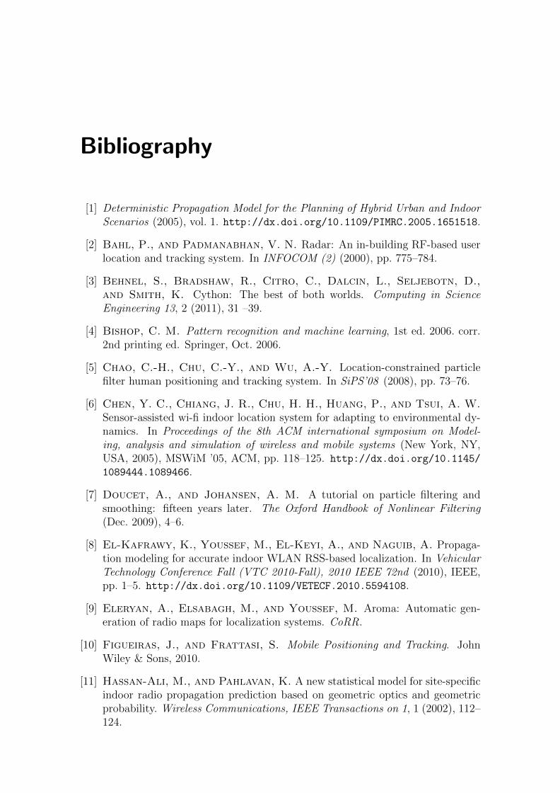
Bibliography
[1] Deterministic Propagation Model for the Planning of Hybrid Urban and IndoorScenarios (2005), vol. 1. http://dx.doi.org/10.1109/PIMRC.2005.1651518.
[2] Bahl, P., and Padmanabhan, V. N. Radar: An in-building RF-based userlocation and tracking system. In INFOCOM (2) (2000), pp. 775–784.
[3] Behnel, S., Bradshaw, R., Citro, C., Dalcin, L., Seljebotn, D.,and Smith, K. Cython: The best of both worlds. Computing in ScienceEngineering 13, 2 (2011), 31 –39.
[4] Bishop, C. M. Pattern recognition and machine learning, 1st ed. 2006. corr.2nd printing ed. Springer, Oct. 2006.
[5] Chao, C.-H., Chu, C.-Y., and Wu, A.-Y. Location-constrained particlefilter human positioning and tracking system. In SiPS’08 (2008), pp. 73–76.
[6] Chen, Y. C., Chiang, J. R., Chu, H. H., Huang, P., and Tsui, A. W.Sensor-assisted wi-fi indoor location system for adapting to environmental dy-namics. In Proceedings of the 8th ACM international symposium on Model-ing, analysis and simulation of wireless and mobile systems (New York, NY,USA, 2005), MSWiM ’05, ACM, pp. 118–125. http://dx.doi.org/10.1145/
1089444.1089466.
[7] Doucet, A., and Johansen, A. M. A tutorial on particle filtering andsmoothing: fifteen years later. The Oxford Handbook of Nonlinear Filtering(Dec. 2009), 4–6.
[8] El-Kafrawy, K., Youssef, M., El-Keyi, A., and Naguib, A. Propaga-tion modeling for accurate indoor WLAN RSS-based localization. In VehicularTechnology Conference Fall (VTC 2010-Fall), 2010 IEEE 72nd (2010), IEEE,pp. 1–5. http://dx.doi.org/10.1109/VETECF.2010.5594108.
[9] Eleryan, A., Elsabagh, M., and Youssef, M. Aroma: Automatic gen-eration of radio maps for localization systems. CoRR.
[10] Figueiras, J., and Frattasi, S. Mobile Positioning and Tracking. JohnWiley & Sons, 2010.
[11] Hassan-Ali, M., and Pahlavan, K. A new statistical model for site-specificindoor radio propagation prediction based on geometric optics and geometricprobability. Wireless Communications, IEEE Transactions on 1, 1 (2002), 112–124.
100 Bibliography
[12] Hatami, A., and Pahlavan, K. Comparative statistical analysis of indoorpositioning using empirical data and indoor radio channel models. In ConsumerCommunications and Networking Conference, 2006. CCNC 2006. 3rd IEEE(Jan. 2006), vol. 2, IEEE, pp. 1018–1022. http://dx.doi.org/10.1109/CCNC.2006.1593192.
[13] Ji, Y., Biaz, S., Pandey, S., and Agrawal, P. Ariadne: a dynamicindoor signal map construction and localization system. In Proceedings of the4th international conference on Mobile systems, applications and services (NewYork, NY, USA, 2006), MobiSys ’06, ACM, pp. 151–164. http://doi.acm.
org/10.1145/1134680.1134697.
[14] Julier, S. J., and Uhlmann, J. K. Unscented filtering and nonlinearestimation. Proceedings of the IEEE 92, 3 (Mar. 2004), 401–422. http:
//dx.doi.org/10.1109/JPROC.2003.823141.
[15] Klepal, M. Novel Approach to Indoor Electromagnetic Wave PropagationModelling. PhD thesis, Czech Technical University, 2003.
[16] Nicoli, M. B. Hmm-based tracking of moving terminals in dense multipathindoorenvironments. Eusipco 2005 (2010).
[17] Pandey, S., Kim, B., Anjum, F., and Agrawal, F. Client assisted locationdata acquisition scheme for secure enterprise wireless networks. vol. 2, pp. 1174–1179 Vol. 2.
[18] Prasithsangaree, P., Krishnamurthy, P., and Chrysanthis, P. Onindoor position location with wireless LANs. vol. 2, pp. 720–724 vol.2.
[19] Pugh, W. Skip lists: a probabilistic alternative to balanced trees. Commun.ACM 33, 6 (June 1990), 668–676. http://dx.doi.org/10.1145/78973.78977.
[20] Richalot, E., Bonilla, M., Wong, M.-F., Fouad-Hanna, V., Bau-drand, H., and Wiart, J. Electromagnetic propagation into reinforced-concrete walls. Microwave Theory and Techniques, IEEE Transactions on 48,3 (Mar. 2000), 357–366. http://dx.doi.org/10.1109/22.826834.
[21] Roweis, S., and Ghahramani, Z. A unifying review of linear gaussianmodels, 1999.
[22] Schmitz, A., Karolski, T., and Kobbelt, L. Using spherical harmonicsfor modeling antenna patterns. IEEE Radio and Wireless Symposium.
[23] Schmitz, A., and Kobbelt, L. Efficient and accurate urban outdoor radiowave propagation. Electromagnetics in Advanced Applications (ICEAA) (Sept.2011), 323–326.
[24] Schmitz, A., and Wenig, M. The effect of the radio wave propagationmodel in mobile ad hoc networks. In MSWiM ’06: Proceedings of the 9th ACMinternational symposium on Modeling analysis and simulation of wireless andmobile systems (New York, NY, USA, 2006), ACM Press, pp. 61–67. http:
//dx.doi.org/10.1145/1164717.1164730.

Bibliography 101
[25] Seitz, J. V. A hidden markov model for pedestrian navigation. PositioningNavigation and Communication, 7th Workshop (Mar. 2010), 120–127.
[26] Valenzuela, R. A ray tracing approach to predicting indoor wireless trans-mission. In Vehicular Technology Conference, 1993 IEEE 43rd (May 1993),IEEE, pp. 214–218. http://dx.doi.org/10.1109/VETEC.1993.507047.
[27] Wallbaum, M., and Wasch, T. Markov localization of wireless local areanetwork clients. In WONS (2004), vol. 2928 of Lecture Notes in ComputerScience, Springer, pp. 1–15.
[28] Wang, H., Szabo, A., Bamberger, J., Brunn, D., and Hanebeck,U. D. Performance comparison of nonlinear filters for indoor WLAN posi-tioning. In Information Fusion, 2008 11th International Conference on (June2008), IEEE, pp. 1–7.
[29] Widyawan, Klepal, M., and Beauregard, S. A backtracking particlefilter for fusing building plans with PDR displacement estimates. 207–212.http://dx.doi.org/10.1109/WPNC.2008.4510376.
[30] Wilson, R. Propagation losses through common building materials 2.4 GHzvs 5 GHz., Aug. 2002.
[31] Woodman, O., and Harle, R. Pedestrian localisation for indoor envi-ronments. In Proceedings of the 10th international conference on Ubiquitouscomputing (New York, NY, USA, 2008), UbiComp ’08, ACM, pp. 114–123.http://dx.doi.org/10.1145/1409635.1409651.
[32] Youssef, M., Mah, M., and Agrawala, A. Challenges: device-free passivelocalization for wireless environments. In MobiCom ’07: Proceedings of the13th annual ACM international conference on Mobile computing and networking(New York, NY, USA, 2007), ACM, pp. 222–229. http://dx.doi.org/10.
1145/1287853.1287880.

102 Bibliography

AAppendix
A.1 List of Abbreviations
AOA Angle Of ArrivalAP Access PointAPI Application Programming InterfaceBRDF Bidirectional Reflectance Distribution FunctionCPU Central Processing UnitGPS Global Positioning SystemGPU Graphics Processing UnitGSM Global System for Mobile CommunicationsHMM Hidden Markov ModelHTTP Hypertext Transfer ProtocolIEEE Institute of Electrical and Electronics EngineersLMSE Least Mean Squared ErrorLOS Line Of SightLDS Linear Dynamic SystemLE Localization ErrorNLOS None Line Of SightOpenGL Open Graphics LibraryOpenMP Open Multi-ProcessingPF Particle FilterPDF Probability Density FunctionRPE Radio Propagation ErrorRSSI Received Signal Strength IndicationSSID Service Set IDentificationSSM Signal Strength MapTDOA Time Difference Of ArrivalTOA Time Of ArrivalUTD Uniform Theory of DiffractionWAF Wall Attenuation Factor
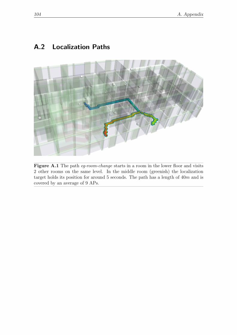
104 A. Appendix
A.2 Localization Paths
Figure A.1 The path eg-room-change starts in a room in the lower floor and visits2 other rooms on the same level. In the middle room (greenish) the localizationtarget holds its position for around 5 seconds. The path has a length of 40m and iscovered by an average of 9 APs.
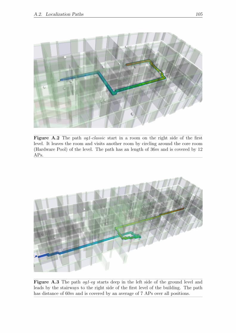
A.2. Localization Paths 105
Figure A.2 The path og1-classic start in a room on the right side of the firstlevel. It leaves the room and visits another room by circling around the core room(Hardware Pool) of the level. The path has an length of 36m and is covered by 12APs.
Figure A.3 The path og1-eg starts deep in the left side of the ground level andleads by the stairways to the right side of the first level of the building. The pathhas distance of 60m and is covered by an average of 7 APs over all positions.
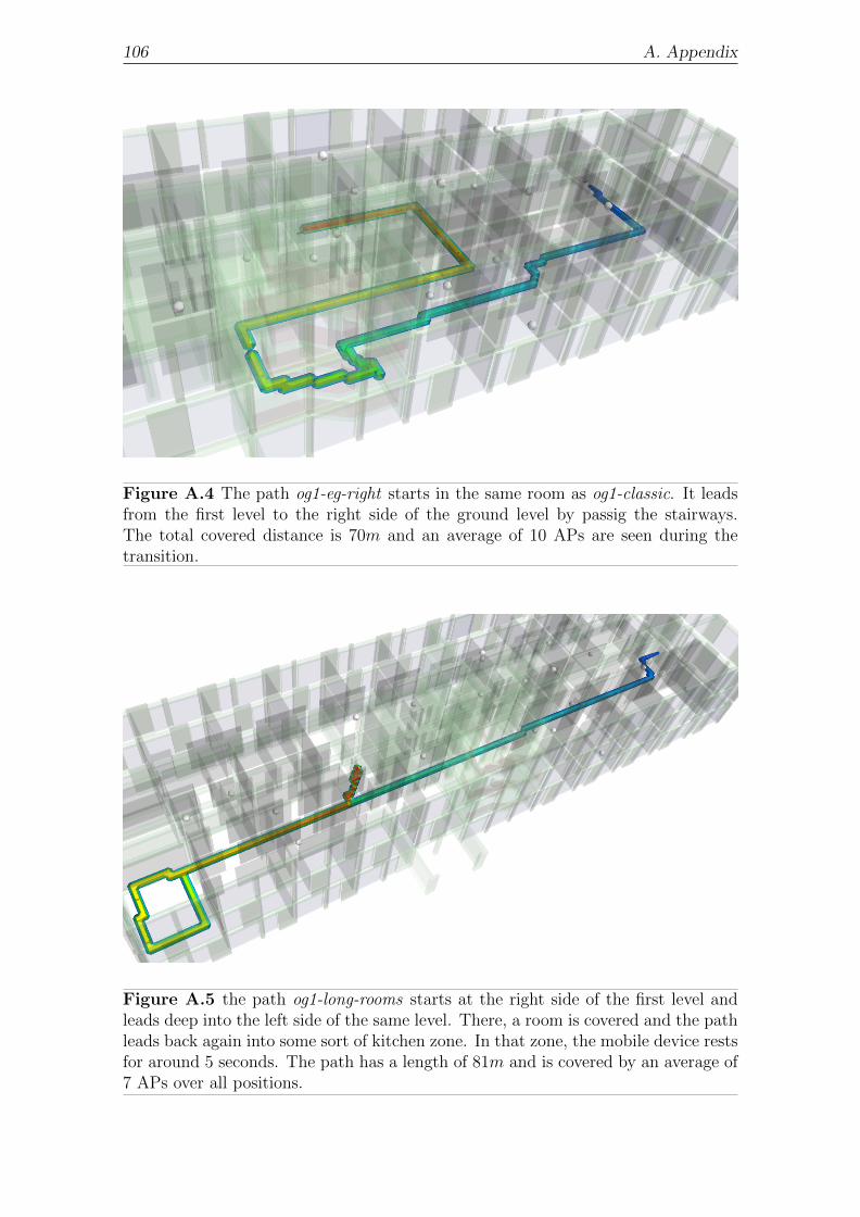
106 A. Appendix
Figure A.4 The path og1-eg-right starts in the same room as og1-classic. It leadsfrom the first level to the right side of the ground level by passig the stairways.The total covered distance is 70m and an average of 10 APs are seen during thetransition.
Figure A.5 the path og1-long-rooms starts at the right side of the first level andleads deep into the left side of the same level. There, a room is covered and the pathleads back again into some sort of kitchen zone. In that zone, the mobile device restsfor around 5 seconds. The path has a length of 81m and is covered by an average of7 APs over all positions.
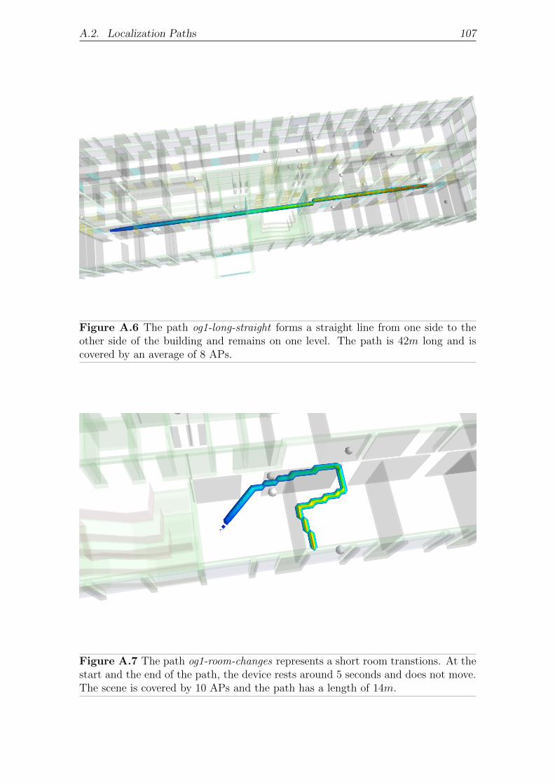
A.2. Localization Paths 107
Figure A.6 The path og1-long-straight forms a straight line from one side to theother side of the building and remains on one level. The path is 42m long and iscovered by an average of 8 APs.
Figure A.7 The path og1-room-changes represents a short room transtions. At thestart and the end of the path, the device rests around 5 seconds and does not move.The scene is covered by 10 APs and the path has a length of 14m.
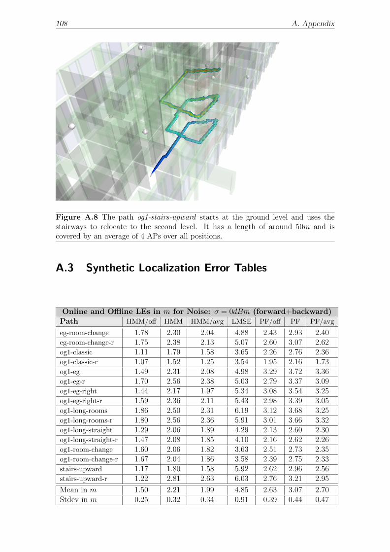
108 A. Appendix
Figure A.8 The path og1-stairs-upward starts at the ground level and uses thestairways to relocate to the second level. It has a length of around 50m and iscovered by an average of 4 APs over all positions.
A.3 Synthetic Localization Error Tables
Online and Offline LEs in m for Noise: σ = 0dBm (forward+backward)Path HMM/off HMM HMM/avg LMSE PF/off PF PF/avg
eg-room-change 1.78 2.30 2.04 4.88 2.43 2.93 2.40eg-room-change-r 1.75 2.38 2.13 5.07 2.60 3.07 2.62og1-classic 1.11 1.79 1.58 3.65 2.26 2.76 2.36og1-classic-r 1.07 1.52 1.25 3.54 1.95 2.16 1.73og1-eg 1.49 2.31 2.08 4.98 3.29 3.72 3.36og1-eg-r 1.70 2.56 2.38 5.03 2.79 3.37 3.09og1-eg-right 1.44 2.17 1.97 5.34 3.08 3.54 3.25og1-eg-right-r 1.59 2.36 2.11 5.43 2.98 3.39 3.05og1-long-rooms 1.86 2.50 2.31 6.19 3.12 3.68 3.25og1-long-rooms-r 1.80 2.56 2.36 5.91 3.01 3.66 3.32og1-long-straight 1.29 2.06 1.89 4.29 2.13 2.60 2.30og1-long-straight-r 1.47 2.08 1.85 4.10 2.16 2.62 2.26og1-room-change 1.60 2.06 1.82 3.63 2.51 2.73 2.35og1-room-change-r 1.67 2.04 1.86 3.58 2.39 2.75 2.33stairs-upward 1.17 1.80 1.58 5.92 2.62 2.96 2.56stairs-upward-r 1.22 2.81 2.63 6.03 2.76 3.21 2.95
Mean in m 1.50 2.21 1.99 4.85 2.63 3.07 2.70Stdev in m 0.25 0.32 0.34 0.91 0.39 0.44 0.47

A.3. Synthetic Localization Error Tables 109
Online and Offline LEs in m for Noise: σ = 4dBm (forward+backward)Path HMM/off HMM HMM/avg LMSE PF/off PF PF/avg
eg-room-change 1.78 2.30 2.04 4.88 2.43 2.93 2.40eg-room-change-r 1.75 2.38 2.13 5.07 2.60 3.07 2.62og1-classic 1.11 1.79 1.58 3.65 2.26 2.76 2.36og1-classic-r 1.07 1.52 1.25 3.54 1.95 2.16 1.73og1-eg 1.49 2.31 2.08 4.98 3.29 3.72 3.36og1-eg-r 1.70 2.56 2.38 5.03 2.79 3.37 3.09og1-eg-right 1.44 2.17 1.97 5.34 3.08 3.54 3.25og1-eg-right-r 1.59 2.36 2.11 5.43 2.98 3.39 3.05og1-long-rooms 1.86 2.50 2.31 6.19 3.12 3.68 3.25og1-long-rooms-r 1.80 2.56 2.36 5.91 3.01 3.66 3.32og1-long-straight 1.29 2.06 1.89 4.29 2.13 2.60 2.30og1-long-straight-r 1.47 2.08 1.85 4.10 2.16 2.62 2.26og1-room-change 1.60 2.06 1.82 3.63 2.51 2.73 2.35og1-room-change-r 1.67 2.04 1.86 3.58 2.39 2.75 2.33stairs-upward 1.17 1.80 1.58 5.92 2.62 2.96 2.56stairs-upward-r 1.22 2.81 2.63 6.03 2.76 3.21 2.95
Mean in m 1.50 2.21 1.99 4.85 2.63 3.07 2.70Stdev in m 0.25 0.32 0.34 0.91 0.39 0.44 0.47
Online and Offline LEs in m for Noise: σ = 8dBm (forward+backward)Path HMM/off HMM HMM/avg LMSE PF/off PF PF/avg
eg-room-change 1.78 2.30 2.04 4.88 2.43 2.93 2.40eg-room-change-r 1.75 2.38 2.13 5.07 2.60 3.07 2.62og1-classic 1.11 1.79 1.58 3.65 2.26 2.76 2.36og1-classic-r 1.07 1.52 1.25 3.54 1.95 2.16 1.73og1-eg 1.49 2.31 2.08 4.98 3.29 3.72 3.36og1-eg-r 1.70 2.56 2.38 5.03 2.79 3.37 3.09og1-eg-right 1.44 2.17 1.97 5.34 3.08 3.54 3.25og1-eg-right-r 1.59 2.36 2.11 5.43 2.98 3.39 3.05og1-long-rooms 1.86 2.50 2.31 6.19 3.12 3.68 3.25og1-long-rooms-r 1.80 2.56 2.36 5.91 3.01 3.66 3.32og1-long-straight 1.29 2.06 1.89 4.29 2.13 2.60 2.30og1-long-straight-r 1.47 2.08 1.85 4.10 2.16 2.62 2.26og1-room-change 1.60 2.06 1.82 3.63 2.51 2.73 2.35og1-room-change-r 1.67 2.04 1.86 3.58 2.39 2.75 2.33stairs-upward 1.17 1.80 1.58 5.92 2.62 2.96 2.56stairs-upward-r 1.22 2.81 2.63 6.03 2.76 3.21 2.95
Mean in m 1.50 2.21 1.99 4.85 2.63 3.07 2.70Stdev in m 0.25 0.32 0.34 0.91 0.39 0.44 0.47
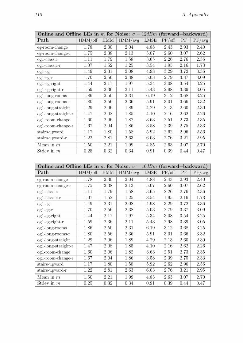
110 A. Appendix
Online and Offline LEs in m for Noise: σ = 12dBm (forward+backward)Path HMM/off HMM HMM/avg LMSE PF/off PF PF/avg
eg-room-change 1.78 2.30 2.04 4.88 2.43 2.93 2.40eg-room-change-r 1.75 2.38 2.13 5.07 2.60 3.07 2.62og1-classic 1.11 1.79 1.58 3.65 2.26 2.76 2.36og1-classic-r 1.07 1.52 1.25 3.54 1.95 2.16 1.73og1-eg 1.49 2.31 2.08 4.98 3.29 3.72 3.36og1-eg-r 1.70 2.56 2.38 5.03 2.79 3.37 3.09og1-eg-right 1.44 2.17 1.97 5.34 3.08 3.54 3.25og1-eg-right-r 1.59 2.36 2.11 5.43 2.98 3.39 3.05og1-long-rooms 1.86 2.50 2.31 6.19 3.12 3.68 3.25og1-long-rooms-r 1.80 2.56 2.36 5.91 3.01 3.66 3.32og1-long-straight 1.29 2.06 1.89 4.29 2.13 2.60 2.30og1-long-straight-r 1.47 2.08 1.85 4.10 2.16 2.62 2.26og1-room-change 1.60 2.06 1.82 3.63 2.51 2.73 2.35og1-room-change-r 1.67 2.04 1.86 3.58 2.39 2.75 2.33stairs-upward 1.17 1.80 1.58 5.92 2.62 2.96 2.56stairs-upward-r 1.22 2.81 2.63 6.03 2.76 3.21 2.95
Mean in m 1.50 2.21 1.99 4.85 2.63 3.07 2.70Stdev in m 0.25 0.32 0.34 0.91 0.39 0.44 0.47
Online and Offline LEs in m for Noise: σ = 16dBm (forward+backward)Path HMM/off HMM HMM/avg LMSE PF/off PF PF/avg
eg-room-change 1.78 2.30 2.04 4.88 2.43 2.93 2.40eg-room-change-r 1.75 2.38 2.13 5.07 2.60 3.07 2.62og1-classic 1.11 1.79 1.58 3.65 2.26 2.76 2.36og1-classic-r 1.07 1.52 1.25 3.54 1.95 2.16 1.73og1-eg 1.49 2.31 2.08 4.98 3.29 3.72 3.36og1-eg-r 1.70 2.56 2.38 5.03 2.79 3.37 3.09og1-eg-right 1.44 2.17 1.97 5.34 3.08 3.54 3.25og1-eg-right-r 1.59 2.36 2.11 5.43 2.98 3.39 3.05og1-long-rooms 1.86 2.50 2.31 6.19 3.12 3.68 3.25og1-long-rooms-r 1.80 2.56 2.36 5.91 3.01 3.66 3.32og1-long-straight 1.29 2.06 1.89 4.29 2.13 2.60 2.30og1-long-straight-r 1.47 2.08 1.85 4.10 2.16 2.62 2.26og1-room-change 1.60 2.06 1.82 3.63 2.51 2.73 2.35og1-room-change-r 1.67 2.04 1.86 3.58 2.39 2.75 2.33stairs-upward 1.17 1.80 1.58 5.92 2.62 2.96 2.56stairs-upward-r 1.22 2.81 2.63 6.03 2.76 3.21 2.95
Mean in m 1.50 2.21 1.99 4.85 2.63 3.07 2.70Stdev in m 0.25 0.32 0.34 0.91 0.39 0.44 0.47
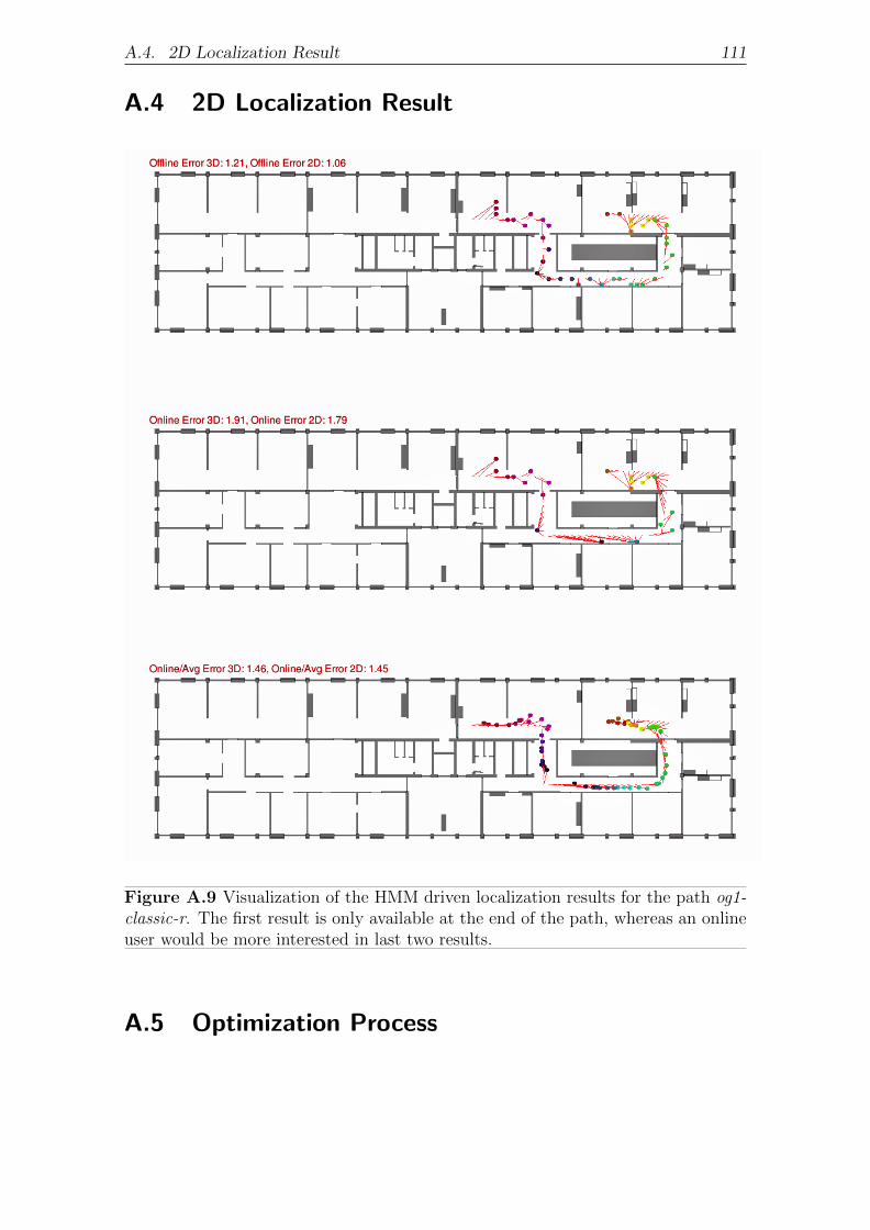
A.4. 2D Localization Result 111
A.4 2D Localization Result
Figure A.9 Visualization of the HMM driven localization results for the path og1-classic-r. The first result is only available at the end of the path, whereas an onlineuser would be more interested in last two results.
A.5 Optimization Process

112 A. Appendix
Figure A.10 Convergence of material parameters during an optimization run withgenetic algorithms. The optimization target can be seen in the upper left corner, itis the average delta between the simulation results and the real world measurements.