indicators for the signal degradation and optimization...
TRANSCRIPT
Indicators for the Signal Degradation and
Optimization of Automotive Radar
Sensors under Adverse Weather Conditions
Vom Fachbereich 18 - Elektrotechnik und Informationstechnikder Technischen Universitat Darmstadt
zur Erlangung der Wurde einesDoktor-Ingenieurs (Dr. -Ing.)
genehmigte
Dissertation
von
Dipl. -Ing. Alebel Arage Hassenaus Worillu / Wollo / Athiopien
Referent: Prof. Dr. -Ing. Rolf JakobyKorreferent: Prof. Dr. -Ing. habil. Peter Knoll
Zeitdauer: 09.2003 - 08.2006Tag der Einreichung: 14.11.2006Tag der Disputation: 18.12.2006
Darmstadt 2006D17
Darmstadter Dissertationen
Abstract
In recent years vehicle radar and lidar sensors are widely used as sourcesof control signals for Autonomous Intelligent Cruise Control and CollisionMitigation systems. These devices are operating in the millimeter waveand infrared range in which their performance may be degraded by adverseweather conditions. Currently available information regarding the signal in-teraction with fog, rain, snow and spray make clear that millimeter-waveradar sensors are far less affected by adverse weather conditions than infrared-based sensors [1, 2, 3, 4]. However, when automotive radar sensors are par-ticularly designed for safety-oriented systems, the effects of critical issues(such as water film and heavy rains) on the sensor performance become ofthe uttermost importance.
In this thesis, an analysis of the effects of water film and rain on millimeter-wave propagation have been presented. Based on the fundamental formula-tion of wave propagation and scattering in stratified as well as random media,physical parameters describing the wave interaction with the water film andrains have been studied and assessed. It has been shown that both signifi-cantly attenuate millimeter-wave signals, and may exert an adverse influenceon detection performance of millimeter-wave radar sensors. Consequently,water-film and rain indicators have been derived from returnedsignals to convey for the first time wet-antenna and rain informa-tion to the radar sensor system, where they could be employed formonitoring the radar detection performance.
Methods have also been worked out in detail for low-cost measure-ment of water-film and rain indicators in the radar system. Experimen-tal investigations have been exhibited to be able to satisfactorily implementthese indicators in production. Finally, techniques have been introducedto show how detection performance could be optimized.
The presented findings emphasize the importance of identification ofwater film and rain and of being able to optimize detection performance inorder to assure availability of automotive radar senors in adverse weatherconditions. Results should also be significant for all kinds of millimeter-waveradar sensors where wave interactions with water film on the surface of theradar antenna or its protecting radome as well as with rains in the radarbeams are the key issue.
Abstract in German
Automotive Radar- und Lidarsensoren werden in den letzten Jahren alsSteuersignalequelle fur Systemen wie Autonomous Intelligent Cruise Control(AICC) und Collision Mitigation (CM) verstarkt eingesetzt. Diese Sensorenoperieren in Millimeterwellen und Infrarotbereich, in welche ihre performanzbei sclechten Wetterverhaltnisse signifikant degradiert werden konnen, undmussen diesen durch geeignetes Design erkannt und angepaßt werden. Beson-ders wichtig fur Millimeterwelle basierten Automotiveradarsensoren ist dieautomatische Erkennung von der Wasserfilm auf der Antennenoberflache unddem Regen im Ubertragungsmedium um die Degradation der Radarsichtweitund -detektionsvermogen dynamisch zu unterdrucken bzw. zu vermeiden. Indieser Dissertationsarbeit werden neueartigen Wasserfilm- und Regenindika-toren vorgestellt, die kostengunstig mit dem am Markt vertretenden Auto-motiveradarsensor von Bosch demonstriert sind und wahrend dieser Arbeitauf Serientauglichkeit untersucht worden. Ferner wird ein Performanzop-timierungsverfahren zur Gewahrleistung der Radarsensorverfugbarkait beischlechtem Wetter presentieren.
Acknowledgments
This work is carried out within the framework of a Ph. D. stipendiumof the Robert Bosch GmbH at the department of Development Long RangeRadar devision of Automotive Electronic Driver Assistance in Leonberg,Baden-Wurttemberg, Germany. Therefore all the persons at this devisionare most gratefully acknowledged.
I wish to express my sincere gratitude to:
My supervisor Professor Dr. -Ing. Rolf Jakoby, for giving me supervisionand inspiration in the Technische Universitat Darmstadt; and co-supervisorProfessor Dr.-Ing. habil. Peter Knoll, for advising and supporting me to con-tinue and complete this Ph. D. work in the Robert Bosch GmbH, Leonberg.
All those who have contributed to this work, and shared their knowledgewith me, here I would like to mention W. M. Steffens, J. Hauk, J. Hilde-brand, T. Binzer and J. Winterhalter.
Those who have helped me with measurements in one or another way:K. D. Mioska, P. Wirth, R. Hermann and D. R. Reddy.
Those who have reviewed this thesis and suggested substantial improvements:A. Damtew and T. Hussien.
My Family and, of course, the almighty God who gave me strength andimperturbability.
Darmstadt, December 2006 Alebel Arage
Contents
1 Introduction 1
2 Wave propagation in stratified and random media 9
2.1 Characteristics of dielectrics . . . . . . . . . . . . . . . . . . . 10
2.2 Wave propagation in stratified media . . . . . . . . . . . . . . 18
2.2.1 Reflection and transmission coefficients . . . . . . . . . 18
2.2.2 Cross-polarization coefficients . . . . . . . . . . . . . . 28
2.3 Wave propagation and scattering in random media . . . . . . 31
2.3.1 Scattering and absorption of a wave by a single particle 31
2.3.2 Basic radar equations . . . . . . . . . . . . . . . . . . . 36
2.3.3 Approximation of average scattered power . . . . . . . 38
3 Automotive radar 43
3.1 Principles of distance and speed measurements . . . . . . . . . 44
3.2 Radar antenna . . . . . . . . . . . . . . . . . . . . . . . . . . 46
3.3 FMCW automotive radar system . . . . . . . . . . . . . . . . 51
4 Effects of water film on millimeter-wave radar 56
4.1 Theoretical analysis . . . . . . . . . . . . . . . . . . . . . . . . 57
i
ii CONTENTS
4.1.1 Wave propagation model . . . . . . . . . . . . . . . . . 57
4.1.2 Derivation of the water-film indicator . . . . . . . . . . 63
4.1.3 Relationship between the water-film effects and theradar maximum detection range . . . . . . . . . . . . . 64
4.2 Experimental investigations . . . . . . . . . . . . . . . . . . . 66
4.2.1 Measurement system . . . . . . . . . . . . . . . . . . . 66
4.2.2 Results and discussions . . . . . . . . . . . . . . . . . . 71
4.3 Investigations of water-film effects on LRR2 sensor . . . . . . 74
4.3.1 Measurement system . . . . . . . . . . . . . . . . . . . 74
4.3.2 Results and discussions . . . . . . . . . . . . . . . . . . 82
5 Effects of rain on millimeter-wave radar 86
5.1 Theoretical analysis . . . . . . . . . . . . . . . . . . . . . . . . 87
5.1.1 Raindrop-size distribution . . . . . . . . . . . . . . . . 87
5.1.2 Total backscattering cross section of rain . . . . . . . . 88
5.2 Experimental investigations of rain effects . . . . . . . . . . . 91
5.2.1 Measurement system . . . . . . . . . . . . . . . . . . . 92
5.2.2 Results and discussions . . . . . . . . . . . . . . . . . . 95
6 Conclusions 102
A Electromagnetic plane Waves 108
B Supplementary Graphs 112
B.1 Attenuation due to hydrometeors . . . . . . . . . . . . . . . . 112
B.2 The complex refraction index of water . . . . . . . . . . . . . 113
B.3 LRR2-transceiver layout . . . . . . . . . . . . . . . . . . . . . 113
CONTENTS iii
B.4 Improvement of SNR due to system adaptation . . . . . . . . 114
B.5 Test car measurement system of an automotive radar sensor . 114
C Glossary 115
C.1 Symbols and physical constants . . . . . . . . . . . . . . . . . 115
C.2 Abbreviations . . . . . . . . . . . . . . . . . . . . . . . . . . . 117
Literature 119
List of Figures
1.1 Possible performance optimization model of an automotiveradar sensor system for safety-oriented applications . . . . . . 7
2.1 Frequency response of permittivity and loss factor for a hypo-thetical dielectric . . . . . . . . . . . . . . . . . . . . . . . . . 13
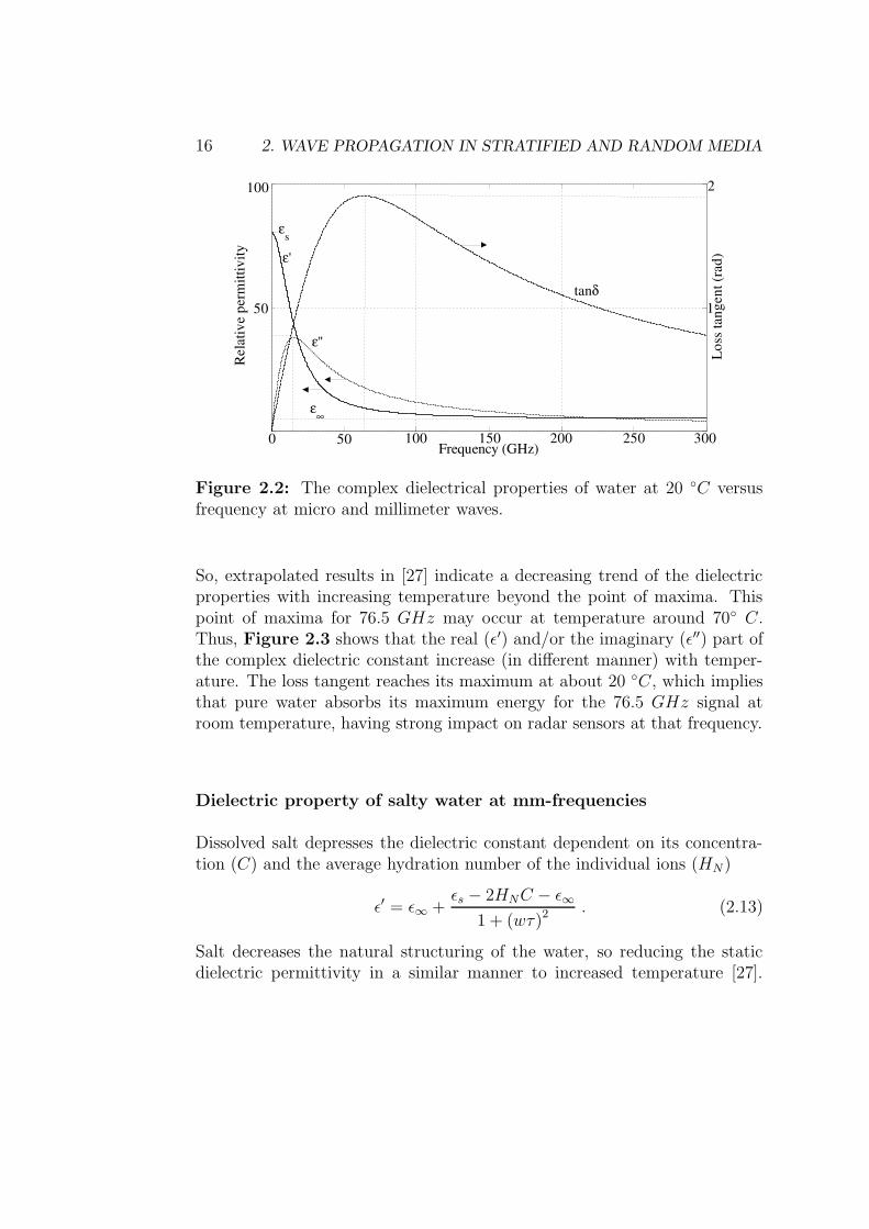
2.2 The complex dielectrical properties of water at 20 C versusfrequency at micro and millimeter waves. . . . . . . . . . . . . 16
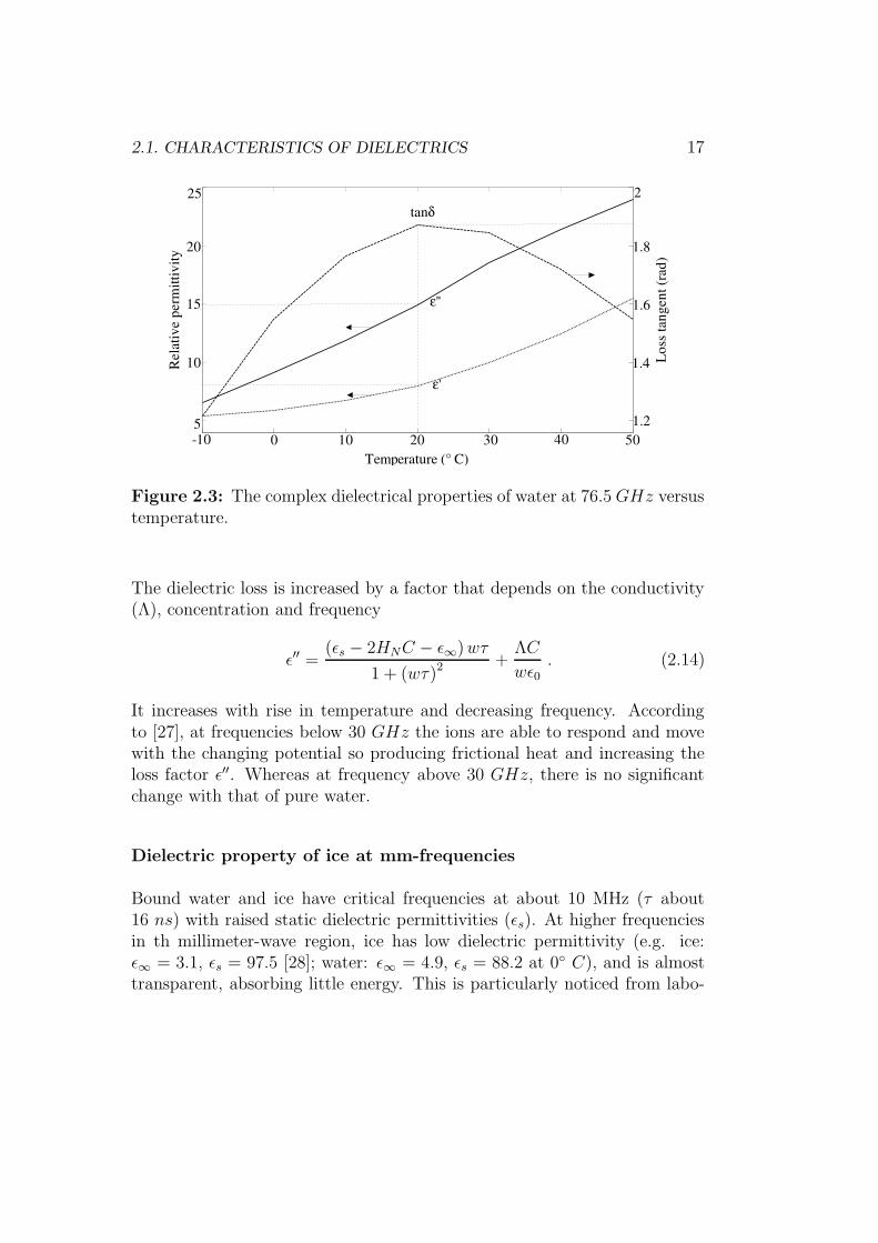
2.3 The complex dielectrical properties of water at 76.5 GHz ver-sus temperature. . . . . . . . . . . . . . . . . . . . . . . . . . 17
2.4 Electromagnetic wave propagation through a stratified media. 19
2.5 A plane wave is incident upon a dielectric scatterer and thescattered field is observed at a distance R . . . . . . . . . . . 32
2.6 Total and absorption cross section normalized to the geometriccross section . . . . . . . . . . . . . . . . . . . . . . . . . . . . 36
2.7 Radar principle. . . . . . . . . . . . . . . . . . . . . . . . . . . 37
2.8 Geometric for single scattering approximation. . . . . . . . . . 39
3.1 Antenna pattern of a homogeneous rectangular aperture . . . 47
3.2 Normalized two-way antenna pattern of the LRR2-Prototype. 48
3.3 Plane-Convex Fresnel lens and its equivalent planar dielectrics. 50
3.4 FMCW automotive radar system with a homodyne receiver . . 52
iv
LIST OF FIGURES v
3.5 FMCW automotive radar modulation scheme . . . . . . . . . 53
3.6 Measurement result with targets at 100 m and 152 m. . . . . . 54
4.1 water film on the surface of radome. . . . . . . . . . . . . . . . 58
4.2 Reflectivity from water film at 20 C. . . . . . . . . . . . . . . 61
4.3 Transmissivity through water film at 20 C. . . . . . . . . . . 62
4.4 Relationship between water-film thickness, reflectivity, trans-missivity and maximum detection range of an automotive radarsensor . . . . . . . . . . . . . . . . . . . . . . . . . . . . . . . 65
4.5 Laboratory measurement system to analyse the effects of waterfilm on a radome at millimeter waves. . . . . . . . . . . . . . . 68
4.6 Transmissivity through tissue paper . . . . . . . . . . . . . . . 69
4.7 Reflectivity of the radome-tissue-paper system versus frequency. 70
4.8 Reflectivity from water film . . . . . . . . . . . . . . . . . . . 72
4.9 Transmissivity through water film . . . . . . . . . . . . . . . . 73
4.10 Measuring system to detect the effects of water film on thesurface of FMCW-automotive radar sensor fitted to the frontof a car. . . . . . . . . . . . . . . . . . . . . . . . . . . . . . . 75
4.11 Polyrod-Patch antenna system of LRR2-Prototype and its equiv-alent transmission line. . . . . . . . . . . . . . . . . . . . . . . 77
4.12 Schematic diagram of FMCW-automotive radar sensor includ-ing external load . . . . . . . . . . . . . . . . . . . . . . . . . 78
4.13 The complex intrinsic impedance of the water film and itsequivalent at the RF-port. . . . . . . . . . . . . . . . . . . . . 80
4.14 Reflectivity from water film and its equivalent at the RF-port. 80
4.15 Calibration curve: operation point of mixer diode versus re-flectivity from water film. . . . . . . . . . . . . . . . . . . . . 81
4.16 Correlation between the distance of radar object and the in-dicator of water film on the surface of radome . . . . . . . . . 83
vi LIST OF FIGURES
4.17 Radar detection capacity versus indicator of water film on thesurface of radar antenna at 76.5 GHz and 20 C. . . . . . . . 84
5.1 Percentage of the total volume contributed by drops of varioussizes for six precipitation rates . . . . . . . . . . . . . . . . . . 87
5.2 Plan view showing narrow beam monostatic radar consistingof raindrop scatterers . . . . . . . . . . . . . . . . . . . . . . . 90
5.3 LRR2 measurement result with targets at 100 m and 152 min dry and rainy weather conditions . . . . . . . . . . . . . . . 92
5.4 Rainfall rate measured on the 29th of July 2005 at the Malmsheimair port, Baden-Wurttemberg, Germany. . . . . . . . . . . . . 94
5.5 Average rain backscattering cross section measured on 29th
July 2005 at the Malmsheim air port, Baden-Wurttemberg,Germany. . . . . . . . . . . . . . . . . . . . . . . . . . . . . . 96
5.6 Rain as extended scatterer in the radar field of view. . . . . . 98
5.7 Four beam average rain backscattering cross section measuredon 29th July 2005 at the Malmsheim air port, Baden-Wurt-temberg, Germany. . . . . . . . . . . . . . . . . . . . . . . . . 99
5.8 Reduction in signal-to-noise ratio due to rain, measured on29th July 2005 at the Malmsheim air port, Baden-Wurttem-berg, Germany. . . . . . . . . . . . . . . . . . . . . . . . . . . 100
5.9 Reduction in signal-to-noise as a function of average rain backscat-tering cross section. . . . . . . . . . . . . . . . . . . . . . . . . 101
B.1 Attenuation of electromagnetic wave through rain and fog . . 112
B.2 Refraction index of water for wavelengths from 10 nm to 10m 113
B.3 Single path layout of the LRR2-Transceiver circuit includingthe load impedance. . . . . . . . . . . . . . . . . . . . . . . . . 113
B.4 Short range SNR improvement by adapting the modulationparameters. . . . . . . . . . . . . . . . . . . . . . . . . . . . . 114

LIST OF FIGURES vii
B.5 Block diagram of the measurement system of an automotiveradar sensor in a test car. . . . . . . . . . . . . . . . . . . . . 114
List of Tables
1.1 Effects of water-particles on the 77 GHz wave propagation . . 5
2.1 Relaxation time (τ) in water as a function of temperature . . 15
3.1 System parameters of the LRR2-Prototype sensor . . . . . . . 55
viii
Chapter 1
Introduction
Motivation
Since 1970 automotive radar sensors have been investigated to use for moreconvenient and safer driving, and have been first employed as cruise controlsystem in the 1980s [5, 6]. This application has been recently spread to Au-tonomous Intelligent Cruise Control (AICC) and Collision Mitigation (CM)systems as a result of cooperate projects between car manufacturers, univer-sities and micro-wave companies. For example, the European project thatstarted in 1986, aimed to improve vehicle safety, efficiency, and economy, wasone of the main driving factor in the development of various types of sensorsfor automobiles, including micro- and millimeter-wave radars.
Furthermore, an Advanced Safety Vehicle Program, started in 1991 un-der the initiative of Japans Transportation Minister, and product road-mapsof automotive system manufacturers show that the incoming trend of thistechnology is focusing at autonomous driving [1, 7]. This may be the ulti-mate form of vehicle dynamics control system. Millimeter-wave radar andvision sensors are parts of the environmental recognition technology that willbe required to achieve effective vehicle dynamics control.
Similar to millimeter-wave radar sensor, infrared-based sensor such as li-dar has been also employed for environmental recognition, particularly for theAdaptive Cruise Control (ACC) system by considering required performanceand feasibility. Both infrared-based and millimeter-wave radar sensors will
1
2 1. INTRODUCTION
provide range, velocity and angle information on targets ahead of the vehicle.This will be used along with vehicle dynamics data to correlate projected ve-hicle path and detected target positions. The resulting data will be used tocontrol the vehicle throttle, brakes, and steering or the automatic transmis-sion. ACC system adapts the speed of the vehicle according to the speed ofthe vehicle ahead, in order to maintain a constant distance between the twovehicles. The driver sets the maximum speed and the minimum separationdesired. Both sensor systems can also be used to locate and track multipletargets on the road ahead, to anticipate traffic conditions in the driving lane.The ACC system application of millimeter-wave and infrared-based sensorsis marketed as a comfort and convenience option rather than a safety option.There is still a safety risk associated with its use on automobiles. Due to thecritical impact of radar and lidar sensors on the ACC system, it is impor-tant to conduct accurate verification and calibration of the system at variousstages of development, production, and installation. Hence, the use of ACCsystems was restricted to highway driving for breaking up to a specified level.If additional breaking is required to slow the automobile, the ACC functionis disabled and the driver has to take control on the automobile.
New generation systems make use of multiple sensors to extend theACC system to city driving or stop-and-go traffic, pre-crash sensing, collisionwarning and avoidance systems (CWAS). These are typically short-range ap-plications and various sensor types can be used, including infrared, vision,ultrasonic, and micro-wave radar. For most applications beyond highwayACC system, multiple sensor systems must be used in conjunction with thelong-range ACC lidar or millimeter-wave radar sensors. Such sensor fusiontechnology is the key to achieve high level environmental recognition and toadvance the target autonomous driving.
Most of these future safety-oriented applications are associated with in-creasing demands for grater performance and reliability in environmentalrecognition sensors at any traffic and weather scenarios. Unfortunately, withmost recent developments and innovative products, such requirements ap-peared not to be met for all weather conditions. This is the challenge forlong-range infrared-based and millimeter-wave radar sensors. As it is indis-pensable for safety-oriented applications, this has to be solved by these sensorengineers. Basically in adverse weather conditions, the electromagnetic waveinteracts not only with hydrometeors (particles of water in solid or liquid
3
form in the atmosphere) but also with materials, which could be built upon the surface of the sensor or its protective covering. Some examples ofhydrometeors are mist, rain, freezing rain, ice pellets, snow, hail and fog.Their sizes are generally 1 µm or more in radius. Expected materials on thesurface of the sensor or its protective covering are like grit and dirt as wellas dray snow and water films, which may be formed through condensation,impingement and stick of water-particles. The wave interaction with thesematerials and hydrometeors also results in attenuation and reflection thatrely on the relationship between the particle-size and the wavelength as wellas on the particle density, extent and index of refraction.
The refractive index of water is rather complicated with a strong tem-perature and frequency dependence. It is given in Figure B.2 in a wideelectromagnetic spectrum. In micro-wave range, the real part is around 10with the imaginary part varying from around 0.2 to 2 but generally ris-ing with temperature and frequency. In millimeter wave range (i.e. above30 GHz), both the real and imaginary parts decrease. So in these both fre-quency ranges, water is known as lossy material. Attenuation due to waterparticle is thus a mixture of absorption and scatter losses. Due to low valueof the imaginary part of the refractive index of water in the region 1 mmto 100 nm, water is transparent at optical frequencies. The attenuation willbe then a result of energy lost through scattering by water particles. Forthe frequency spectrum above 10 GHz, the attenuation of electromagneticenergy due to water particles is presented in Figure B.1.
The different forms of water-particles (mist, rain, freezing rain, ice pel-lets, snow, hail and fog) affect the infrared and millimeter-wave propagationunequally. The reason is that the absorption and total scattering cross sec-tions of the water-particle depend on the relationship between particle-sizeand wavelength as well as on the particle density and extent [2, § 3-2].
A very big fraction of the water-particles in the atmosphere has generallya diameter greater than ≥ 2 µm. For example, fog droplets are smaller than100 µm in diameter and the number density may vary from 106 to 109 m−3
with typical value of 108 m−3. The water content may vary from 0.03 g/m3
for light fog to 2 g/m3 for heavy fog, and optical visibility may be typically1 km down to 30 m.Raindrops, as the second example of water-particles in the atmosphere, arerandomly positioned in space with a special drop size distribution that de-
4 1. INTRODUCTION
pends on the rainfall intensity. They have generally diameters greater than(100 µm up to 4mm). Laws and Parsons give an empirical raindrop-sizedistribution for a mean drop-size spectrum in continental temperate rainfall(Figure 5.1). It shows that a very big fraction of the raindrops at rainfallintensities 2.5 mm/hr and larger have a diameter greater than or equal to1 mm.
Almost all sizes of these water-particles are greater than the infraredwavelengths (λ ≤ 30 µm). They may consequently yield maximum scatter-ing cross sections (Figure 2.6) in the infrared and visible light range. Thisresults in quit large attenuation and backscattered signal, particularly indense water-particles like heavy rain and fog droplets (Figure B.1). Theseintelligibly degrads the performance of lidar sensor (λ ≤ 1 µm) not onlyby limiting the maximum detection range to that of comparable human eye,but also by increasing process occupies nontrivial amounts of memory andcomputational throughput to filter out irrelevant detections due to water-particles.
This also includes road spray that could arise during rainy weather con-dition from other road vehicles in front of the sensor-carrier vehicle [3]. Notethat, due to beam spreading loss and scattering in the propagation path, onlybackscattered signals from road spray and water-drops in the near distancehave considerable effect on the sensor performance.
In the millimeter-wave range, only raindrops with rainfall intensitiesgreater than 4 mm/hr (Figure 5.1) can obtain maximum absorption andtotal scattering cross sections. This may introduce strong rain attenuationand backscattering. The effects of snow and hail are difficult to assess pre-cisely since their water content varies significantly. In general, ice has a muchsmaller loss than water of the same mass, and millimeter-wave attenuationin dry snow is hence negligible [2, § 3-2]. If the snow is wet, however, the at-tenuation increases considerably but expected to be less than moderate rain.It all implies that the 77 GHz millimeter-wave radar may operate withoutany substantial degradation of performance in all forms of water-particlesexcept rains with rainfall intensities ≥ 4 mm/hr (i.e moderate, heavy andextremely heavy rains).
As previously pointed out, water has a high dielectric constant and is alossy material at micro-wave and millimeter-wave range. In the case of water
5
film on the surface of antenna or its radome, this may well provide enoughattenuation and reflection according to the water-film thickness or amountof water content as well as frequency. It means, particularly for millimeterwaves, a less degree of moisture on the surface of antenna lens or radome canadversely affect wave propagation and introduce ceasing of millimeter-waveradar operation.
On the other hand, lidar sensor is insensible to water film because of thepure dielectric property of water at optical frequencies. Nevertheless, dustmaterials like dry snow, grit and dirt on the lidar lens may also cause harmon measurement sensitivity due to attenuation and diffraction phenomena[8, § 14.5].
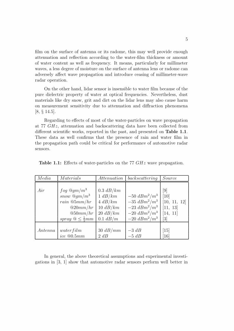
Regarding to effects of most of the water-particles on wave propagationat 77 GHz, attenuation and backscattering data have been collected fromdifferent scientific works, reported in the past, and presented on Table 1.1.These data as well confirms that the presence of rain and water film inthe propagation path could be critical for performance of automotive radarsensors.
Table 1.1: Effects of water-particles on the 77 GHz wave propagation.
Media Materials Attenuation backscattering Source
Air fog @gm/m3 0.3 dB/km [9]snow @gm/m3 1 dB/km −50 dBm2/m3 [10]rain @5mm/hr 4 dB/km −35 dBm2/m3 [10, 11, 12]
@20mm/hr 10 dB/km −23 dBm2/m3 [11, 13]@50mm/hr 20 dB/km −20 dBm2/m3 [14, 11]
spray @ ≤ 12mm 0.1 dB/m −20 dBm2/m3 [3]
Antenna waterfilm 30 dB/mm −3 dB [15]ice @0.5mm 2 dB −5 dB [16]
In general, the above theoretical assumptions and experimental investi-gations in [3, 1] show that automotive radar sensors perform well better in
6 1. INTRODUCTION
most adverse weather conditions than lidar sensors. Further improvement ofthis favorable aspect should make millimeter wave based automotive radarsensors reliable in all weather conditions.
Hence, this work has been focused more on the fundamental understand-ing of how water film and heavy rains affect the performance of millimeter-wave automotive radar sensors and how this could be recognized as well ascounterbalanced, automatically. With a greater knowledge about these ef-fects, the requirements of future advanced safety application systems (i.e.better performance and reliability at all weather conditions) may be sub-stantially achieved by the millimeter-wave radar sensor.
Objectives
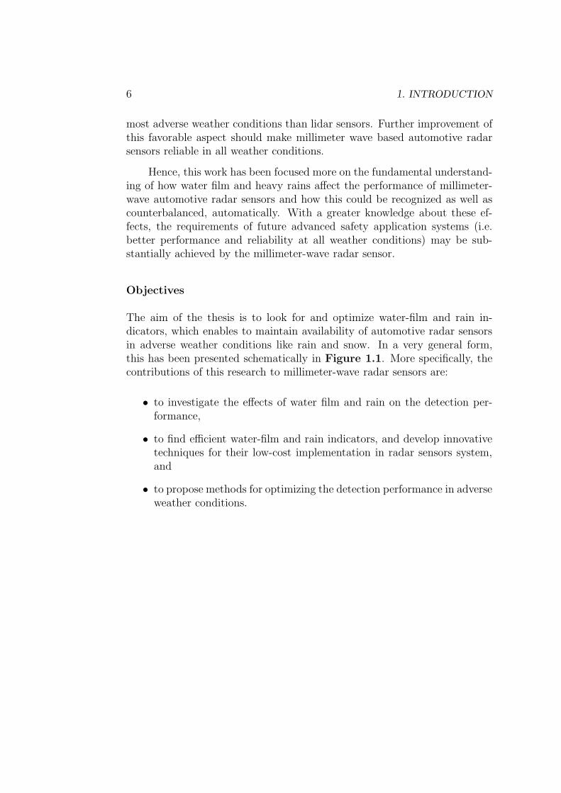
The aim of the thesis is to look for and optimize water-film and rain in-dicators, which enables to maintain availability of automotive radar sensorsin adverse weather conditions like rain and snow. In a very general form,this has been presented schematically in Figure 1.1. More specifically, thecontributions of this research to millimeter-wave radar sensors are:
• to investigate the effects of water film and rain on the detection per-formance,
• to find efficient water-film and rain indicators, and develop innovativetechniques for their low-cost implementation in radar sensors system,and
• to propose methods for optimizing the detection performance in adverseweather conditions.
7
Performance analysis
Counter-measures
Indicators
Internal causes of signal degradation
External causes of signal degradation
System interruption
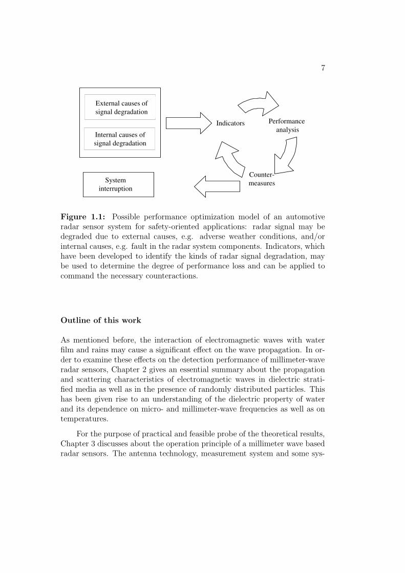
Figure 1.1: Possible performance optimization model of an automotiveradar sensor system for safety-oriented applications: radar signal may bedegraded due to external causes, e.g. adverse weather conditions, and/orinternal causes, e.g. fault in the radar system components. Indicators, whichhave been developed to identify the kinds of radar signal degradation, maybe used to determine the degree of performance loss and can be applied tocommand the necessary counteractions.
Outline of this work
As mentioned before, the interaction of electromagnetic waves with waterfilm and rains may cause a significant effect on the wave propagation. In or-der to examine these effects on the detection performance of millimeter-waveradar sensors, Chapter 2 gives an essential summary about the propagationand scattering characteristics of electromagnetic waves in dielectric strati-fied media as well as in the presence of randomly distributed particles. Thishas been given rise to an understanding of the dielectric property of waterand its dependence on micro- and millimeter-wave frequencies as well as ontemperatures.
For the purpose of practical and feasible probe of the theoretical results,Chapter 3 discusses about the operation principle of a millimeter wave basedradar sensors. The antenna technology, measurement system and some sys-
8 1. INTRODUCTION
tem parameters of an actual automotive long range radar sensor have beenreviewed in brief.
The main essence of this thesis is concentrated in Chapter 4 and Chapter5. The theoretical analysis as well as the experimental and practical investi-gation of the effects of water film on millimeter-wave propagation have beentreated in Chapter 4. Physical parameters such as reflectivity and transmis-sivity have been adapted with lossy stratified media, and used to describethe effects of water film on detection performance of millimeter-wave radarsensors. A water-film indicator has been derived from the correlation of thesephysical parameters and its relationship with the maximum detection rangeof a radar sensor has been worked out in detail. Results have been thenverified with a number of experimental investigations. The electronic versionof this work includes lab and on-road demonstrations of these results usingan actual automotive radar sensor systems.
Chapter 5 deals with the theoretical and practical analysis of the effectsof rain on the detection performance of millimeter-wave radar sensors. Thetheoretical analysis of effects of rain has been treated using results revised inChapter 2. Particularly, the backscattering effect of rain has been examinedfor narrow beam monostatic radars using the first order multiple scatteringprinciple. This covers the practical situation like deriving of rain indicatorfrom backscattered signal in order to identify rain and its consequence onthe detection performance of automotive radar sensors. The relationship be-tween the loss of signal-to-noise ratio and rain backscattering cross sectionhas been also elaborated. The investigation have been supported with prac-tical experiments by comparing measurement results of an actual automotiveradar sensor system and meteorological instrumentation like rain gauge.
In a compact form, Chapter 6 summarizes the essential results of thiswork. Further aspects regarding to performance optimization of automotiveradar sensors have been also mentioned briefly.
Chapter 2
Wave propagation in stratifiedand random media
Before beginning discussions about the effects of water film and rain on theperformance of millimeter-wave radar sensors and their identification mech-anism, this chapter gives an essential summary about the propagation andscattering characteristics of electromagnetic waves in multi-layer media aswell as in the presence of randomly distributed particles.
First, it deals with isotropic linear media, giving physical explanationsfor electric responses. Lossy materials, particularly water with dielectricproperties that depends upon frequency and temperature, will be describedsuccinctly using the Debye-model. And then, it demonstrates how physi-cal parameters like reflectivity and transmissivity of stratified media can bedetermined using the fundamental formulation of the electromagnetic wavetheory.
Finally it revises basic radar equations and examines the scattering andabsorption properties of randomly distributed particles using single and first-order multiple scattering approximations. The results of these theoreticalanalysis will be directly applied in the upcoming chapters to illustrate effectsof water film and rain on the performance of millimeter-wave radar sensors.
9
10 2. WAVE PROPAGATION IN STRATIFIED AND RANDOM MEDIA
2.1 Characteristics of dielectrics
The response of materials to applied electromagnetic field includes displace-ments of both free and bound electrons by electric fields and the orientation ofatomic moments by magnetic fields. These responses can be mostly treatedas linear (i.e. proportional to the applied fields) over useful range of fieldmagnitudes. Often, the response is independent of the direction of the ap-plied field and such material is called isotropic. The frequency of the fieldcounts to one of the key factors, which may significantly influence the reac-tion of these linear, isotropic materials to time-varying fields. Hence, it isof special importance to discuss the frequency dependence of permittivity,defined as the ability of a material to respond to the electric field.
Isotropic and linear materials have been considered in this text, andthey are represented by scalar values of ε and µ (usual dielectrics µ = µ0) foranalysis at a given frequency. As they are given in several books and articles[17, 18, 19, 20, 21], various physical phenomena contributing to the complexpermittivity differ for solids, liquids and gases. Nevertheless, some of thefundamental properties and simple models will be discussed to give insightinto the most important characteristics [22, 8].It can be shown that, if the atoms or molecules are polarized, a dipole momentdensity can be defined by
Pd =lim
∆V → 0
∑
i pi
∆V. (2.1)
Neglecting higher-order multi-poles, this is identical to the so called electricalpolarization that enters the relation between the electric flux density D andthe electric field vector E
D = ε0E + P = ε0 (1 + χe)E . (2.2)
The term ε0 = 8.85 × 10⁻¹²F/m is the ability of a free space to store elec-trostatic energy (permittivity of free space), χe is the dielectric susceptibilityand it has been assumed that P is linearly dependent on the E. Few dielec-tric materials, such as polar dielectrics, have a permanent polarization thatretards the orientation of the dipole molecules in the applied electric field E.If there are N like molecules per unit volume, the induced polarization Pmay be written
P = ε0χeE = NgαTE , (2.3)
2.1. CHARACTERISTICS OF DIELECTRICS 11
where αT is the molecular polarizability and g is the ratio between localfield acting on the molecule and the applied field E. The local field differsfrom the applied field because of the effect of surrounding molecules. Thecorresponding electric flux density may also be written
D = εE = ε0εrE . (2.4)
So, comparing (2.4) with (2.2) and (2.3) gives the relative permittivity
εr = 1 +NgαT
ε0= 1 + χe . (2.5)
If the surrounding molecules act in a spherically symmetric fashion on themolecule for which the local electric field is being calculated, g can be shownto be (2+εr)
3and (2.5) may then be written as
εr − 1
εr + 2=NαT
3ε0. (2.6)
This expression is known as the Clausius-Mossotti relation, or when fre-quency effects in αT are included, the Debye equation [22, p. 669]. It isproved to be accurate for gases, and gives qualitative behavior for liquidsand gases.
The molecular polarizability αT has contributions from several differentatomic or molecular effects. One part, called electronic, arises from the shiftof electron cloud in each atom relative to its positive nucleus. Another part,called ionic, comes from the displacement of positive and negative ions fromtheir neutral position. Still another part may arise if the individual moleculeshave permanent dipole moments. Application of the electric field tends toalign these permanent dipoles against the randomizing forces of molecularcollision, and since random motion is a function of temperature, this effectis clearly temperature dependent. The three effects together constitute thetotal molecular polarizability,
αT = αe + αi + αd . (2.7)
Where αe, αi, αd are electronic, ionic and permanent dipole contribution,respectively. The dependence of the molecular polarization and of the relativepermittivity on the frequency of the applied field constitute the phenomenonof dispersion, which needs deeply the atomic theory of matter for an adequate
12 2. WAVE PROPAGATION IN STRATIFIED AND RANDOM MEDIA
treatment. But in [22, 8], the Lorentz model of an atom gives a simplifiedmodel of a dispersing medium and explicit dependence of the complex relativepermittivity εr on frequency.
In the general characterization of lossy dielectrics, the complex relativepermittivity εr is defined as:
ε = ε0εr = ε0 (ε′ − jε′′) = ε0ε′ (1 − jε′′/ε′) = ε0ε
′ (1 − jtan δ) . (2.8)
Where ε′ is the ability of the material to be polarized by the external electricfield, and ε′′ and tan δ are the loss factor and loss tangent, respectively. Theloss tangent quantifies the efficiency with which the electromagnetic energyis converted to heat.
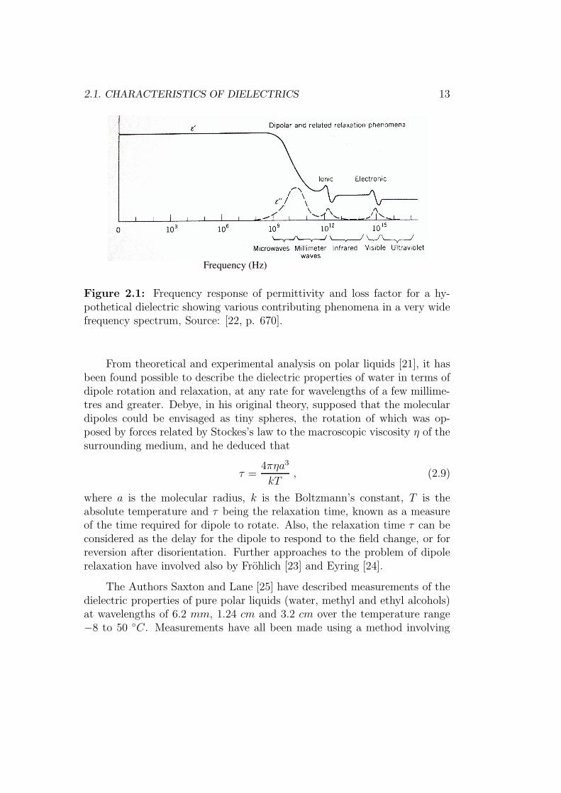
The molecular polarization contributes to ε′ and ε′′ in a manner shown bythe electronic and ionic resonances pictured as well as by dipole orientationand relaxation for a hypothetical dielectric in Figure 2.1. In case of ionicand electronic contribution, the lossy part (near resonance) goes through apeak. The contribution to ε′ from a given resonance (like the reactance ofthe tuned circuit [22, Chap. 11]) has peaks of the opposite sign on either sideof the resonance. These contribution plays no part at frequencies of interestto this work.The dynamic response of the permanent dipole contribution to permittivityis different in that the force opposing complete alignment of the dipoles in thedirection of the applied field is from thermal effects. It acts as a viscous forceand the dynamic response is ”overdamped” and produce smooth decreasein ε along with a peak of absorption (Figure 2.1). Since this contributionis depend to a significant extent upon frequency and temperature, the nextparagraph discusses in detail about the dielectric properties of polar materialslike water at millimeter-frequencies.
Dielectric property of water at mm-frequencies
As it is explained above, the knowledge of the dielectric properties of lossymaterials, of which water is an example, is important in the study of millimeter-wave propagation. From this point of view the observation of dielectric prop-erties of water at different temperatures including supercooled water is of in-terest, since water in these state often occurs in rain, slushes, ice and cloudsfrom which radar signal may be attenuated.
2.1. CHARACTERISTICS OF DIELECTRICS 13
Frequency (Hz)
Figure 2.1: Frequency response of permittivity and loss factor for a hy-pothetical dielectric showing various contributing phenomena in a very widefrequency spectrum, Source: [22, p. 670].
From theoretical and experimental analysis on polar liquids [21], it hasbeen found possible to describe the dielectric properties of water in terms ofdipole rotation and relaxation, at any rate for wavelengths of a few millime-tres and greater. Debye, in his original theory, supposed that the moleculardipoles could be envisaged as tiny spheres, the rotation of which was op-posed by forces related by Stockes’s law to the macroscopic viscosity η of thesurrounding medium, and he deduced that
τ =4πηa3
kT, (2.9)
where a is the molecular radius, k is the Boltzmann’s constant, T is theabsolute temperature and τ being the relaxation time, known as a measureof the time required for dipole to rotate. Also, the relaxation time τ can beconsidered as the delay for the dipole to respond to the field change, or forreversion after disorientation. Further approaches to the problem of dipolerelaxation have involved also by Frohlich [23] and Eyring [24].
The Authors Saxton and Lane [25] have described measurements of thedielectric properties of pure polar liquids (water, methyl and ethyl alcohols)at wavelengths of 6.2 mm, 1.24 cm and 3.2 cm over the temperature range−8 to 50 C. Measurements have all been made using a method involving
14 2. WAVE PROPAGATION IN STRATIFIED AND RANDOM MEDIA
the observation of the attenuation in transmission through wave guides ofdiffering cross-section dimensions containing the liquid. The complex relativedielectric constant εr of a medium is related to the refractive index n andabsorption coefficient κ as follows:
εr = ε′ − jε′′ = (n− jκ)2 . (2.10)
One could then determine both ε′ and ε′′, and therefore also refractive indexn and the absorption coefficient κ, for water from these measurements ofthe rate of attenuation in transmission through two wave guides of suitablychosen cross-section dimension. According to (2.9), τ varies with temperaturein a manner which can be obtained from the well-known Debye expressionfor the dielectric constant of a polar medium in a time-dependent fields:
ε′ = ε∞ +εs − ε∞
1 + (wτ)2 , (2.11)
ε′′ =(εs − ε∞)wτ
1 + (wτ)2 . (2.12)
In equations (2.11) and (2.12) εs is the relative permittivity measured at lowfrequencies (or static dielectric constant), ε∞ is that part of the dielectricconstant due to the electronic and atomic polarizations, w = 2πf , where f isthe frequency. The measurements given in [25] have made it possible to finda single value of ε∞ = 4.9, substantially independent of temperature, anda single relaxation time for any given temperature which will satisfactorilyaccount for the dielectric properties of water at millimetre and centimetrewavelengths. In addition, it has been established that agreement betweentheory and experiment is satisfactory down to a wavelength of 6 mm, andalso shown that the dielectric properties of water vary in a continuous mannerthrough the normal freezing-point (0 C) into the supercooled state down totemperatures of the order of −8 C. Based on the value τ and measured dataof εs (see Table 2.1), the components of the complex relative permittivityof pure water and its corresponding loss tangent have been calculated formicro- and millimeter-wave range using (2.11), (2.12) and (2.8).
Results are provided to Figure 2.2 for a temperature of 20 C. Thedielectric loss factor ε′′ increases to a maximum at the critical frequencywτ = 1 ⇒ fc = 1
2πτ, where the first derivation of (2.12) gets minimum.
For water at 20 C and τ = 10.1 ps, the loss factor reaches its maximum
2.1. CHARACTERISTICS OF DIELECTRICS 15
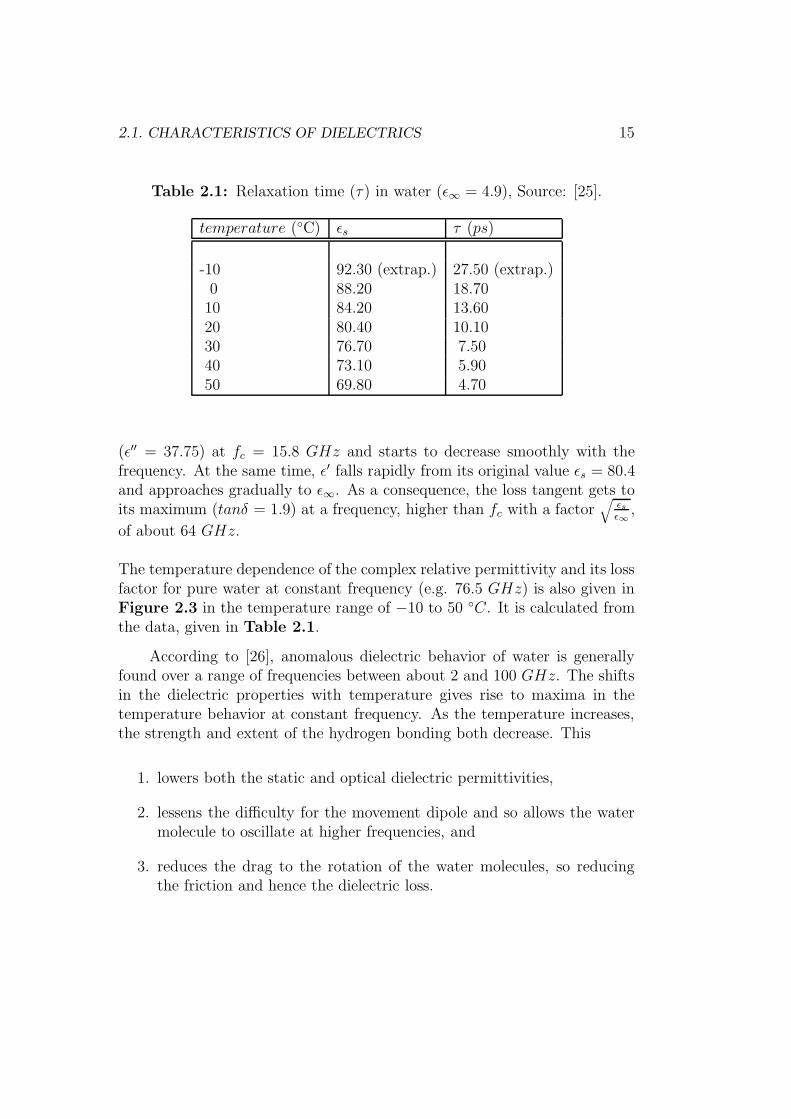
Table 2.1: Relaxation time (τ) in water (ε∞ = 4.9), Source: [25].
temperature (C) εs τ (ps)
-10 92.30 (extrap.) 27.50 (extrap.)0 88.20 18.70
10 84.20 13.6020 80.40 10.1030 76.70 7.5040 73.10 5.9050 69.80 4.70
(ε′′ = 37.75) at fc = 15.8 GHz and starts to decrease smoothly with thefrequency. At the same time, ε′ falls rapidly from its original value εs = 80.4and approaches gradually to ε∞. As a consequence, the loss tangent gets toits maximum (tanδ = 1.9) at a frequency, higher than fc with a factor
√
εs
ε∞,
of about 64 GHz.
The temperature dependence of the complex relative permittivity and its lossfactor for pure water at constant frequency (e.g. 76.5 GHz) is also given inFigure 2.3 in the temperature range of −10 to 50 C. It is calculated fromthe data, given in Table 2.1.
According to [26], anomalous dielectric behavior of water is generallyfound over a range of frequencies between about 2 and 100 GHz. The shiftsin the dielectric properties with temperature gives rise to maxima in thetemperature behavior at constant frequency. As the temperature increases,the strength and extent of the hydrogen bonding both decrease. This
1. lowers both the static and optical dielectric permittivities,
2. lessens the difficulty for the movement dipole and so allows the watermolecule to oscillate at higher frequencies, and
3. reduces the drag to the rotation of the water molecules, so reducingthe friction and hence the dielectric loss.
16 2. WAVE PROPAGATION IN STRATIFIED AND RANDOM MEDIA
Frequency (GHz)
Rel
ativ
e pe
rmitt
ivity
Los
s ta
ngen
t (ra
d)
tanδ
ε''
ε'
εs
ε∞
100
50
50 100 150 200 250 300
2
1
0
Figure 2.2: The complex dielectrical properties of water at 20 C versusfrequency at micro and millimeter waves.
So, extrapolated results in [27] indicate a decreasing trend of the dielectricproperties with increasing temperature beyond the point of maxima. Thispoint of maxima for 76.5 GHz may occur at temperature around 70 C.Thus, Figure 2.3 shows that the real (ε′) and/or the imaginary (ε′′) part ofthe complex dielectric constant increase (in different manner) with temper-ature. The loss tangent reaches its maximum at about 20 C, which impliesthat pure water absorbs its maximum energy for the 76.5 GHz signal atroom temperature, having strong impact on radar sensors at that frequency.
Dielectric property of salty water at mm-frequencies
Dissolved salt depresses the dielectric constant dependent on its concentra-tion (C) and the average hydration number of the individual ions (HN)
ε′ = ε∞ +εs − 2HNC − ε∞
1 + (wτ)2 . (2.13)
Salt decreases the natural structuring of the water, so reducing the staticdielectric permittivity in a similar manner to increased temperature [27].
2.1. CHARACTERISTICS OF DIELECTRICS 17
Temperature (° C)
Rel
ativ
e pe
rmitt
ivity
Los
s ta
ngen
t (ra
d)
tanδ
ε'
ε''
25
20
15
10
5-10 0 10 20 30 40 50
2
1.8
1.6
1.4
1.2
Figure 2.3: The complex dielectrical properties of water at 76.5GHz versustemperature.
The dielectric loss is increased by a factor that depends on the conductivity(Λ), concentration and frequency
ε′′ =(εs − 2HNC − ε∞)wτ
1 + (wτ)2 +ΛC
wε0. (2.14)
It increases with rise in temperature and decreasing frequency. Accordingto [27], at frequencies below 30 GHz the ions are able to respond and movewith the changing potential so producing frictional heat and increasing theloss factor ε′′. Whereas at frequency above 30 GHz, there is no significantchange with that of pure water.
Dielectric property of ice at mm-frequencies
Bound water and ice have critical frequencies at about 10 MHz (τ about16 ns) with raised static dielectric permittivities (εs). At higher frequenciesin th millimeter-wave region, ice has low dielectric permittivity (e.g. ice:ε∞ = 3.1, εs = 97.5 [28]; water: ε∞ = 4.9, εs = 88.2 at 0 C), and is almosttransparent, absorbing little energy. This is particularly noticed from labo-
18 2. WAVE PROPAGATION IN STRATIFIED AND RANDOM MEDIA
ratory measurements, which have been made and published by a number ofresearchers at millimeter and sub-millimeter wavelengths [2, 29].
2.2 Wave propagation in stratified media
The subject of stratified media has been very extensively treated in the sci-entific literature and many schemes for the computation of its optical effectshave been proposed [30, 8, 31, 22]. In this section, based on the basic proper-ties of the electromagnetic filed [8, Chap. 1], the theory of stratified media isdiscussed for treating a model having small number of layers. Some specialcases of particular interest of this work is also considered in detail. Onlydielectric stratified media will be treated in this section. The extension ofthe analysis to lossy media will be described in Chapter 4, in accordancewith the effects of water film on the performance of millimeter wave radarsensors.
The notation introduced in this section will be used throughout thisthesis. Cartesian coordinates x, y, z and unit vectors ex, ey, ez have beenchosen. A medium whose properties are constant throughout each planeperpendicular to a fixed direction is called a stratified medium. If the z-axisof a Cartesian reference system is taken along this special direction, then
ε = ε(z), µ = µ(z) . (2.15)
2.2.1 Reflection and transmission coefficients
Consider a linearly polarized, simple harmonic plane wave (see A) of ampli-tude E0 incident upon a stratified medium that extends from z = 0 to z = d2
and that is bounded on each side by a homogeneous, semi-infinite mediumair (Figure 2.4). When an incident plane wave Ei falls on to a boundarybetween two homogeneous media of different dielectric properties, it is splitinto two waves: a transmitted wave proceeding into the second medium anda reflected wave propagated back into the first medium. The existence ofthese two waves can be demonstrated from the boundary condition, since itis easily seen that these conditions cannot be satisfied without postulatingboth the transmitted and the reflected wave. Let be tentatively assume that
2.2. WAVE PROPAGATION IN STRATIFIED MEDIA 19
these waves are also plane so that expression for their directions of propa-gation and their amplitude shall be driven according to (A.14) and (A.18).
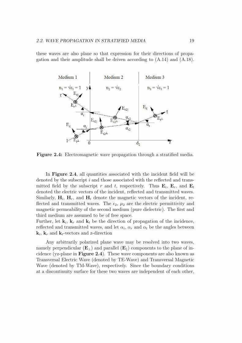
Figure 2.4: Electromagnetic wave propagation through a stratified media.
In Figure 2.4, all quantities associated with the incident field will bedenoted by the subscript i and those associated with the reflected and trans-mitted field by the subscript r and t, respectively. Thus Ei, Er, and Et
denoted the electric vectors of the incident, reflected and transmitted waves.Similarly, Hi, Hr, and Ht denote the magnetic vectors of the incident, re-flected and transmitted waves. The ε2, µ2 are the electric permittivity andmagnetic permeability of the second medium (pure dielectric). The first andthird medium are assumed to be of free space.Further, let ki, kr and kt be the direction of propagation of the incidence,reflected and transmitted waves, and let αi, αr and αt be the angles betweenki, kr and kt-vectors and z-direction
Any arbitrarily polarized plane wave may be resolved into two waves,namely perpendicular (E⊥) and parallel (E‖) components to the plane of in-cidence (yz-plane in Figure 2.4). These wave components are also known asTransversal Electric Wave (denoted by TE-Wave) and Transversal MagneticWave (denoted by TM-Wave), respectively. Since the boundary conditionsat a discontinuity surface for these two waves are independent of each other,
20 2. WAVE PROPAGATION IN STRATIFIED AND RANDOM MEDIA
they will have different expressions for reflection and transmission of electro-magnetic wave in dielectric medium. Therefore, the expression for reflectionand transmission factor of electromagnetic wave could be separately treatedfor perpendicular and parallel components of the propagated wave.The total reflection and transmission factor will be then obtained by super-position of these results.
Perpendicular Polarized Wave (TE-Wave)
Medium 1: the incident electric field vector Ei⊥ is directed towardsthe x-axis of the Cartesian coordinate system and makes an angle of incidenceαi between its propagation direction ki and the z-axis of the incidence plane(Figure 2.4). So, the normal and radius vector of this incidence field willbe
ηi = eysinαi + ezcosαi , (2.16)
andri = eyy + ezz . (2.17)
Substituting equations (2.16) and (2.17) into the first term of equations(A.23) and (A.24) give the incident electric and magnetic field vectors forthe first medium:
Ei⊥ = exE0e−jk(ysinαi+zcos αi) , (2.18)
Hi⊥ = (eycosαi − ezsinαi)E0
Z0e−jk(ysin αi+zcos αi) . (2.19)
The reflected wave from the boundary of the first and second medium makesan angle of reflection αr with the negative z-axis of the incidence plane byits propagation back into the first medium so that it obtains a normal vector
ηr = eysinαr − ezcosαr . (2.20)
According to the second term of equations (A.23) and (A.24), the reflectedelectric and magnetic field vectors for the first medium will be
Er⊥ = exr⊥E0e−jk(ysin αr−zcosαr) , (2.21)
and
Hr⊥ = −(eycosαr + ezsinαr)r⊥E0
Z0
e−jk(ysin αr−zcos αr) , (2.22)
where r⊥ is the complex reflection coefficient.
2.2. WAVE PROPAGATION IN STRATIFIED MEDIA 21
Medium 2: the transmitted wave across the boundary of medium 1and 2 makes an angle of transmission αt2 with respect to the positive z-axisby its propagation toward medium 3 so that it obtain the following normaland field vectors
ηt2 = eysinαt2 + ezcosαt2 , (2.23)
Et2⊥ = exAt2⊥E0e−jkn2(ysinαt2+zcos αt2) , (2.24)
Ht2⊥ = (eycosαt2 − ezsinαt2)n2At2⊥E0
Z0
e−jkn2(ysin αt2+zcos αt2) , (2.25)
where n2 is the index of refraction of the second medium and At2⊥ is acomplex amplitude of the Et2 that splits into reflected and transmitted waveat transition of the medium 2 and 3. The reflected wave, propagate back tothe medium 2, makes an angle of reflection αr2 with z-axis and will gain anormal and field vectors of
ηr2 = eysinαr2 − ezcosαr2 , (2.26)
Er2⊥ = exAr2⊥E0e−jkn2(ysin αr2−zcos αr2) , (2.27)
Hr2⊥ = − (eycosαr2 + ezsinαr2)n2Ar2⊥E0
Z0
e−jkn2(ysin αr2−zcos αr2) , (2.28)
where Ar2⊥ is the complex amplitude of the reflected electric field Er2.
Medium 3: it includes only the wave that refracts through the bound-ary of medium 2 and 3 and continue to propagate in the direction of αt withrespect to the positive z-axis. Its normal and field vectors will be then
ηt = eysinαt + ezcosαt , (2.29)
Et⊥ = ext⊥E0e−jk(ysin αt+zcos αt) , (2.30)
Ht⊥ = (eycosαt − ezsinαt)t⊥E0
Z0e−jk(ysin αt−zcos αt) , (2.31)
where t⊥ is a complex transmission coefficient for medium 2.
Equations for electric and magnetic field vectors of medium 1 to 3 arestated due to theirs continuous physical properties, characterized by the εand µ. These properties change abruptly at the transition between the me-dia (Figure 2.4). As a result, the vectors E, H, D and B may then be
22 2. WAVE PROPAGATION IN STRATIFIED AND RANDOM MEDIA
expected also to become discontinuous, while the charge and current densitywill degenerate into corresponding surface quantity. Note that the electricdisplacement D and the magnetic induction B are known as the second setof vectors, which describe the effects of the field on material objects (see A).Relations from boundary conditions, describing the transitions across suchdiscontinuity surfaces, will be therefore used as follows [8, Chap. 1]. The tan-gential component of the electric and magnetic field vectors are continuousacross the surface. Hence, it gives at the boundary where z = 0:
Ei⊥(0) + Er⊥(0) = Et2⊥(0) + Er2⊥(0) , (2.32)
Hi⊥y(0) + Hr⊥y(0) = Ht2⊥y(0) + Hr2⊥y(0) . (2.33)
Where the index y in (2.33) implies the y-component of the magnetic vectorthat is tangential to the y-x plane boundary whereas the z-component of themagnetic vector is normal to the y-x plane boundary.Substituting equations (2.18), (2.21), (2.24), (2.27) into equation (2.32) andequations (2.19), (2.22), (2.25), (2.28) into equation (2.33) yield
e−jky sinαi + r⊥e−jky sinαr = At2⊥e
−jkn2ysin αt2 + Ar2⊥e−jkn2ysin αr2 , (2.34)
and
ey
(
cosαie−jky sin αi − r⊥cosαre
−jky sin αr
)
=
eyn2
(
At2⊥cosαt2e−jkn2y sin αt2 − Ar2⊥cosαr2e
−jkn2y sinαr2
)
. (2.35)
In a homogeneous medium, since the incident and reflected wave normals arein the plane of incidence, the law of reflection can be applied to the aboveequations. That is, regarding to Figure 2.4
αi = αr, αt2 = αr2 = α2 . (2.36)
Also, equations (2.34) and (2.35) become true for the whole y-axis and showthat the refracted wave normal is in the plane of incidence, as well
sinαi = n2 sinα2 . (2.37)
Equation (2.37) is known as the law of refraction (or Snell’s law) [22, 8]. Sim-ilarly, the continuity of tangential components of the electric and magneticfield vectors at the transition between medium 2 and 3 (z = d2) demands
Et2⊥(d2) + Er2⊥(d2) = Et⊥(d2) , (2.38)
2.2. WAVE PROPAGATION IN STRATIFIED MEDIA 23
andHt2⊥y(d2) + Hr2⊥y(d2) = Ht⊥y(d2) . (2.39)
The following expressions will be obtained by substituting equations (2.24),(2.27), (2.30) into equation (2.38) and equations (2.25), (2.28), (2.31) intoequation (2.39), and by considering the law of reflection (2.36)
(
At2⊥e−jkn2d2 cos α2 + Ar2⊥e
jkn2d2 cos α2
)
e−jkn2y sinα2 =
t⊥e−jk(y sin αt+d2 cos αt), (2.40)
and
eyn2cosα2
(
At2⊥e−jkn2d2 cos α2 − Ar2⊥e
jkn2d2 cos α2
)
e−jkn2y sin α2 =
eycosαtt⊥e−jk(y sin αt−d2 cos αt) . (2.41)
The fulfillment of the above two equation along the y-axis requires the rela-tion
n2sinα2 = sinαt , (2.42)
and it yields in combination with (2.37) the general law of refraction forFigure 2.4
sinαi = n2sinα2 = sinαt . (2.43)
Equation (2.43) implies that the wave, passing through Figure 2.4, continuesits propagation in medium 3 with the same direction of propagation as theincident wave in the first medium, i.e. αi = αt.Substituting the expressions (2.36) and (2.43) into (2.34), (2.35), (2.40) and(2.41) yields a simplified linear equation system from which the four unknowncomplex quantities r⊥, At2⊥, Ar2⊥ and t⊥ may be obtained.
1 + r⊥ = At2⊥ + Ar2⊥ , (2.44)
cosαi (1 − r⊥) = n2 cosα2 (At2⊥ − Ar2⊥) , (2.45)
At2⊥e−jkn2d2 cos α2 + Ar2⊥e
jkn2d2 cos α2 = t⊥e−jkd2 cos αt , (2.46)
n2cosα2
(
At2⊥e−jkn2d2 cos α2 − Ar2⊥e
jkn2d2 cos α2
)
= t⊥cosαte−jkd2 cos αt .
(2.47)
These linear equation systems, (2.44) to (2.47), can be easily extendedfor stratified media with more than three layers, and used to formulate equa-tions for the total reflection and total transmission coefficients, as it is used
24 2. WAVE PROPAGATION IN STRATIFIED AND RANDOM MEDIA
in § 4.1. The relationship between the number of layers (NL) and the numberof linear equation (NLE) to be obtained is given by NLE = 2 ∗NL− 2.
Equations (2.44) to (2.47) may be conveniently expressed in terms of r⊥and t⊥ associated with the perpendicular components of the reflection andtransmission coefficients of the second medium in Figure 2.4. In terms ofthese expression, the formula for r⊥ and t⊥ become
r⊥ =j(
Q
n2
− n2
Q
)
sin δ
2cos δ + j(
Qn2
+ n2
Q
)
sin δ, (2.48)
t⊥ =2ejδ0
2cos δ + j(
Qn2
+ n2
Q
)
sin δ, (2.49)
whereQ =
cosαi
cosα2=
cosαi√
1 − sin2 αi
ε2
, (2.50)
is the relation between angle of incidence and angle of transmission, and
δ = kn2d2 cosα2 = kd2
√
n22 − sin2 αi, δ0 = kd2 cosαi ,
(2.51)
are phase terms. The expressions in (2.48) and (2.49) show that the complexreflection and transmission coefficients of a stratified medium depend on theangle of incidence, the electrical properties of the material, the frequency ofthe incident wave and the thickness of the stratified medium. That means,these expressions may be utilized to study the effects of materials, such asice- and water film on the antenna surface of automotive radar, on the radiowave propagation (see chapter 4).The phase terms in (2.48) and (2.49) are known as phase change on reflectionand on transmission, whilst the magnitudes represent the absolute value ofthe reflected and transmitted fields. Squaring the magnitude in (2.48) and(2.49) give the reflection and transmission coefficient of the power.
R⊥ = |r⊥|2 =(Q2 − ε2)
2sin2 δ
4ε2Q2 + (Q2 − ε2)2sin2 δ ,
(2.52)
T⊥ = |t⊥|2 =4ε2
4ε2 +(
Q2−ε2Q
)2sin2 δ
, (2.53)
2.2. WAVE PROPAGATION IN STRATIFIED MEDIA 25
where R⊥ and T⊥ are called the reflectivity and transmissivity, associatedwith polarization in the perpendicular direction, respectively. It can easilybe verified that, in agreement with the law of conservation of energy,
R⊥ + T⊥ = 1 . (2.54)
According to (2.52), the dielectric film in Figure 2.4 will be reflection freeonly by sin δ = 0, i.e for the following thicknesses of the stratified medium(see (2.51))
d2 =m
2
λ√
ε2 − sin2 αi
, m = 0, 1, 2, ...
.
(2.55)
In such cases, the amount of the power of the incident field transmit com-pletely to the third semi-infinite medium. The maximum reflection and min-imum transmission are to expect by sin δ = 1, i.e. for the film with thethicknesses of
d2 =2m+ 1
4
λ√
ε2 − sin2 αi
, m = 0, 1, 2, ...
.
(2.56)
According to (2.52), (2.53) and (2.50), the magnitude for the maximum re-flection and minimum transmission will be
|r⊥|max =ε2 −Q2
ε2 +Q2=
ε2 − 1
ε2 + 1 − 2 sin2 αi ,
(2.57)
|t⊥|min =2√ε2Q
ε2 +Q2=
2cosαi
√ε2 − sinαi
ε2 + 1 − 2sin2 αi .
(2.58)
Parallel Polarized Wave (TM Wave)
In case of TM wave, the electric field vector of the incident wave Ei⊥ (2.18)rotates an its wave normal by 90 and become the following direction ofpolarization in the incidence plane
ηi × ex = ey cosαi − ez sinαi .(2.59)
26 2. WAVE PROPAGATION IN STRATIFIED AND RANDOM MEDIA
Therefore, it has been denoted in Fig 2.4 by E‖. The corresponding magneticfield vector will be then, according to A.19, polarized in the perpendicular(or positive x) direction to the plane of incidence. It is then referred astransversal magnetic (TM) wave.
The corresponding formula for reflection and transmission coefficients ofTM wave are immediately obtained by using the similar strategy and takingsame procedures like the TE wave. Therefore, the tangential component ofthe electric and magnetic field vectors, are continuous across the surface,given at the boundary where z = 0:
(
1 + r‖)
cosαi =(
At2‖ + Ar2‖)
cosα2 , (2.60)
1 − r‖ = n2
(
At2‖ − Ar2‖)
, (2.61)
and at the boundary z = d2
cosα2
(
At2‖e−jδ + Ar2‖e
jδ)
= t‖cosαie−jδ0 , (2.62)
n2
(
At2‖e−jδ − Ar2‖e
jδ)
= t‖e−jδ0
.(2.63)
Where r‖, t‖ are the complex reflection and transmission coefficients, associ-ated with the parallel polarized wave components of the stratified medium,and At2‖, Ar2‖ are the complex amplitudes for the forward and backwardpropagated wave in the stratified medium of Figure 2.4. The required r‖and t‖ may then be obtained from the linear equation systems (2.60) to (2.63)with the help of (2.50) and (2.51)
r‖ =j(
1Qn2
−Qn2
)
sin δ
2cos δ + j(
1Qn2
+Qn2
)
sin δ, (2.64)
t‖ =2ejδ0
2cos δ + j(
1Qn2
+Qn2
)
sin δ. (2.65)
The above expressions show that r‖ and t‖ can be obtained from r⊥ andt⊥ if the term Q in (2.48) and (2.49) is substituted with 1
Q, which implies
specially for the r‖ a possible change in phase. According to (2.64), thereflection coefficient will be zero not only for sin δ = 0 but also for εQ2 = 1.
2.2. WAVE PROPAGATION IN STRATIFIED MEDIA 27
It will be achieved if the wave is incident under the so called polarizing orBrewster angle, denoted by αB and will be determine by substituting Q from(2.50):
αB = arctan√ε2 . (2.66)
The electric vector of the reflected wave has no component in the plane ofincidence at αB and it will appear again for angle of incidence beyond αB
with a change in phase or polarization with respect to that of the incidencewave [8, p. 43-49] [32, §. 21-4].Similar to r⊥ and t⊥, the maximum reflection and minimum transmissioncoefficients of the TM wave are to expect by sin δ = 1, i.e. for the thicknessesof the film given by (2.56). The expression for these terms can be hold thenfrom (2.64) and (2.65):
∣
∣
∣r‖∣
∣
∣
max=
|ε2Q2 − 1|ε2Q2 + 1
=
∣
∣
∣ε2 (ε2 − 1) − (ε22 − 1) sin2 αi
∣
∣
∣
ε2 (ε2 + 1) − (ε22 + 1) sin2 αi
, (2.67)
∣
∣
∣t‖∣
∣
∣
min=
2√ε2Q
ε2Q2 + 1=
2ε2cosαi
√
ε2 − sin2 αi
ε2 (ε2 + 1) − (ε22 + 1) sin2 αi
. (2.68)
The reflectivity R‖ and transmissivity T‖, associated with polarization in theparallel direction, expressed in terms of the magnitude of r‖ and t‖ as follows:
R‖ =∣
∣
∣r‖∣
∣
∣
2=
(
ε2Q− 1Q
)2sin2 δ
4ε2 +(
ε2Q− 1Q
)2sin2 δ
, (2.69)
T‖ =∣
∣
∣t‖∣
∣
∣
2=
4ε2
4ε2 +(
ε2Q− 1Q
)2sin2 δ
. (2.70)
Analogous to (2.54), expression (2.69) and (2.70) verifies also the fulfillmentof law of conservation of energy for a dielectric medium:
R‖ + T‖ = 1 . (2.71)
According to Figure 2.4, the E vector of the incident wave that is the resul-tant electric field vector of Ei‖ and Ei⊥, makes an angle of ψ with the planeof incidence, yz-plane. This angle is known as a polarization angle for thelinear polarized wave E. Finally, the total reflectivity R and transmissivity
28 2. WAVE PROPAGATION IN STRATIFIED AND RANDOM MEDIA
T of the two secondary fields, i.e. Er and Et, may be expressed in terms ofthe polarization angle ψ and R⊥, R‖ and T⊥, T‖, respectively [8, p. 43-49]:
R = R‖cos2 ψ +R⊥sin2 ψ , (2.72)
T = T‖cos2 ψ + T⊥sin2 ψ . (2.73)
For normal incidence, i.e. for αi = 0, the distinction between the paralleland perpendicular components disappears, and one has from (2.52), (2.69)and (2.53), (2.70)
R = R‖ = R⊥ =(ε2 − 1)2sin2 δ
4ε2 + (ε2 − 1)2sin2 δ, (2.74)
T = T‖ = T⊥ =4ε2
4ε2 + (ε2 − 1)2sin2 δ. (2.75)
It is to see from (2.74) that the smaller the difference in the dielectric proper-ties of the stratified medium and its surrounding, the less the energy carriedaway by the reflected wave.
The above results will be generally applied in chapter 4 to observe thesignificance of effects of materials on the millimeter-wave propagation, whenthey may be appeared in the propagation path. The relationship betweenpower loss and power transmitted, particularly due to lossy materials on theantenna surface of automotive radars, can be clearly and easily stated usingequations (2.74) and (2.75).
2.2.2 Cross-polarization coefficients
The reflected and transmitted wave are described not only by their amplitudeand phase, but also by their polarization (see § 2.2.1). One of the most diffi-cult problems connected with propagation of wave through stratified mediais the question of what happens to the original polarization of the incidentwave after the wave has been reflected and transmitted.
On the basis of theoretical work, Beckmann and Spizzichino showedthat a wave reflected in the plane of incidence is not depolarized if the in-cident wave is polarized either purely vertically or horizontally. Further, onthe basis of theoretical studies, it was shown there that a horizontally or
2.2. WAVE PROPAGATION IN STRATIFIED MEDIA 29
vertically polarized wave is strongly depolarized if it is scattered out of theplane of incidence, for example laterally. All these and a detail treatmentof depolarization caused by a surface of arbitrary dielectric property havebeen illustrated in [33, Chap. 8] and show in the general case a change inpolarization must be expected.
The cross-polarization factor uniquely defines the orthogonal polariza-tion to which an electromagnetic wave is subjected. It is useful only if Ei
is linearly polarized. In Figure 2.4, the incidence wave Ei is assumed tobe linearly polarized and makes an angle of polarization ψ with the plane ofincidence, yz-plane. Its unit vector e0 lies in the plane, which is stretchedout on ex and ηi × ex, and may be expressed in terms of ψ and (2.16)
e0 = excosψ + (eycosαi − ezsinαi) sinψ . (2.76)
As consequence, the amplitude of the incidence wave E0, the reflected waveEr and the transmitted wave Et may take a form of expression like:
E0 = (Ecosψ) ex + (Esinψ) (eycosαi − ezsinαi) , (2.77)
Er = (r⊥Ecosψ) ex +(
r‖Esinψ)
(eycosαi − ezsinαi) , (2.78)
Et = (t⊥Ecosψ) ex +(
t‖Esinψ)
(eycosαi − ezsinαi) . (2.79)
As it has been seen in §2.2.1, the reflection coefficients r⊥ and r‖ as well ascorresponding transmission coefficients t⊥ and t‖ are the same in amplitudeand phase only for a normal incidence, i.e. αi = 0. In all other cases,they are completely different in amplitude and phase. Hence the reflectedand transmitted waves are polarized elliptically. The orthogonally polarizedelectric field Ek lies in the direction of a unit vector
ek = ηi × e0 , (2.80)
and obtains the following expression for its reflexion and transmission wavecomponents
Erk = ek ·Er, Etk = ek · Et . (2.81)
By substituting (2.78), (2.79), (2.80) into (2.81) and by considering equa-tions (2.16), (2.48), (2.49), (2.64), (2.65), and (2.76), the cross-polarizationcoefficients for reflection pkr and transmission pkt will be given in relation tothe amplitude of the incidence wave E:
pkr =Erk
E=
1
2|sin 2ψ|
∣
∣
∣r⊥ − r‖∣
∣
∣ , (2.82)
30 2. WAVE PROPAGATION IN STRATIFIED AND RANDOM MEDIA
pkt =Etk
E=
1
2|sin 2ψ|
∣
∣
∣t‖ − t⊥∣
∣
∣ . (2.83)
According to (2.82) and (2.83), the cross-polarization coefficients will bemaximum for a ψ = 45 deg linear polarized incidence wave and be minimum(or zero) for a purely parallel polarized (ψ = 90 deg) or purely perpendicularpolarized (ψ = 0 deg) incidence waves, as mentioned in [33]. For a 45 deglinear polarized incidence wave, (2.82) and (2.83) become then
pkrmax =1
2
∣
∣
∣r⊥ − r‖∣
∣
∣ , (2.84)
pktmax =1
2
∣
∣
∣t‖ − t⊥∣
∣
∣ . (2.85)
There will also no cross-polarization (or depolarization) if r⊥ = r‖ and/ort⊥ = t‖, as it may be seen from (2.84) and (2.85). The only important case ofthis is near normal incidence, i.e. αi = 0 or sin δ = 0 (see (2.48), (2.64) as wellas (2.49), (2.65)). For sin2 δ = 1, substituting equations (2.57) and (2.67)in (2.84) as well as (2.58) and (2.68) in (2.85) give on the other hand thefollowing general formulas for the maximum cross-polarization coefficients ofreflection and transmission
pkrmax =
∣
∣
∣
∣
∣
ε2 (1 −Q4)
(ε2 +Q2)(ε2Q2 + 1)
∣
∣
∣
∣
∣
, (2.86)
pkrmax =
∣
∣
∣
∣
∣
√ε2 (ε2 − 1)Q (1 −Q2)
(1 + ε2Q2)(ε2 +Q2)
∣
∣
∣
∣
∣
. (2.87)
For 45 deg linearly polarized incidence wave, these equations show that thecross-polarization is mainly a function of dielectric properties and angle ofincidence. Its significance and applicability will be thus examined in therelation with the effects of lossy materials on the electromagnetic wave prop-agation, specially in Chapter 4 for the identification of water film at theantenna surface of automotive radar sensors.
2.3. WAVE PROPAGATION AND SCATTERING IN RANDOM MEDIA 31
2.3 Wave propagation and scattering in
random media
The propagation and scattering characteristics of a wave in the presence ofrandomly distributed particles has been exhaustively covered in a number ofbooks [2, 34]. This section thus summarizes only the basic formulations of thescattering problems, which are principally basic for the potential applicationsin the upcoming chapters of this work.
Random scatterers are random distributions of many particles (or dis-crete scatterers). Some examples are rain, fog, smog, hail, and other particlesin a state of Brownian motion. These media are, in general, randomly vary-ing in time and space so that the amplitude and phase of the waves mayalso fluctuate randomly in time and space. These random fluctuations andscattering of the waves are important in a variety of practical problems. Forexample, radar engineers may need to concern themselves with clutter echoesproduced by storms, rain, snow, or hail.
Wave propagation and scattering analysis in such random media can bemade in two steps. First, by considering the scattering and absorption char-acteristics of a single scatterer, and second, by considering the characteristicsof a wave when many scatterers are distributed randomly. The next sectiondiscusses in brief the definitions of scattering amplitude, and absorption andscattering cross-sections.
2.3.1 Scattering and absorption of a wave by a single
particle
The single scattering theory is applicable to the waves in a thin diameterdistribution of scatterers. This covers many practical situations includingradar, lidar, and sonar (sound navigation ranging) applications in variousmedia.
When a single particle is illuminated by a wave, a part of the incidentpower is scattered out and another part is absorbed by the particle. Thecharacteristics of these two phenomena, scattering and absorption, can beexpressed most conveniently by assuming an incident plane wave, discussed
32 2. WAVE PROPAGATION IN STRATIFIED AND RANDOM MEDIA
Ei(r)
R
ηi
ηs
Particleε(r), µ0 ε0, µ0
Es(r)
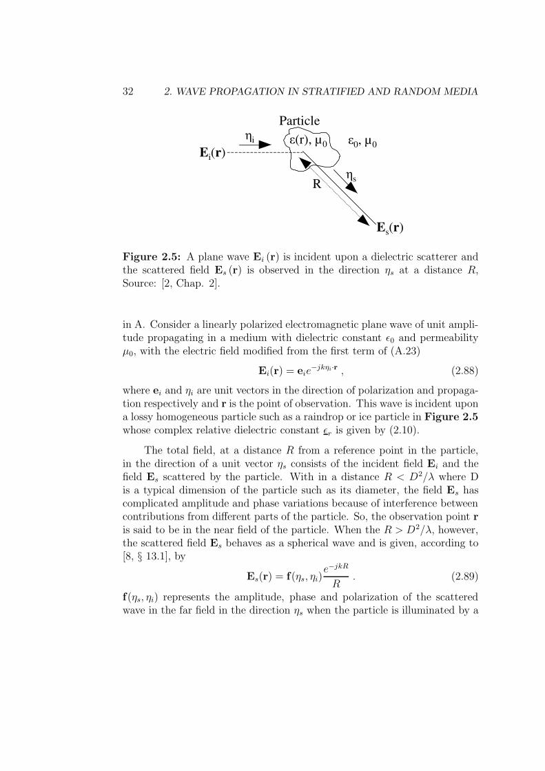
Figure 2.5: A plane wave Ei (r) is incident upon a dielectric scatterer andthe scattered field Es (r) is observed in the direction ηs at a distance R,Source: [2, Chap. 2].
in A. Consider a linearly polarized electromagnetic plane wave of unit ampli-tude propagating in a medium with dielectric constant ε0 and permeabilityµ0, with the electric field modified from the first term of (A.23)
Ei(r) = eie−jkηi·r , (2.88)
where ei and ηi are unit vectors in the direction of polarization and propaga-tion respectively and r is the point of observation. This wave is incident upona lossy homogeneous particle such as a raindrop or ice particle in Figure 2.5whose complex relative dielectric constant εr is given by (2.10).
The total field, at a distance R from a reference point in the particle,in the direction of a unit vector ηs consists of the incident field Ei and thefield Es scattered by the particle. With in a distance R < D2/λ where Dis a typical dimension of the particle such as its diameter, the field Es hascomplicated amplitude and phase variations because of interference betweencontributions from different parts of the particle. So, the observation point ris said to be in the near field of the particle. When the R > D2/λ, however,the scattered field Es behaves as a spherical wave and is given, according to[8, § 13.1], by
Es(r) = f(ηs, ηi)e−jkR
R. (2.89)
f(ηs, ηi) represents the amplitude, phase and polarization of the scatteredwave in the far field in the direction ηs when the particle is illuminated by a
2.3. WAVE PROPAGATION AND SCATTERING IN RANDOM MEDIA 33
plane wave propagating in the direction ηi with unit amplitude. It is knownas the scattering amplitude. It should be also noted that even though theincident wave is linearly polarized, the scattered wave is in general ellipticallypolarized [35].
The exact expression of the scattering amplitude is the volume integralof the multiplication of the total electric field inside the particle and therelative dielectric property [2, § 2-4]. A quantity which is often of interestin the analysis of scattering experiments is not the scattered field itself butrather the rate at which the energy is scattered and absorbed by the particle.It turns out that there is a close relationship between the rate at whichenergy is lost from the incident field by these processes and the amplitudeof the scattered field in the forward direction (the direction incidence). Thisrelationship is quantitatively expressed by the so called optical cross-sectiontheorem [8, § 13.3 and 13.6.3].
Consider the scattered power flux density Ss at a distance R from theparticle in the direction ηs, caused by an incident power flux density Si. Theirratio σd defins the differential scattering cross section of the particle per unitsolid angle at distance R. According to equations (A.22), (2.88) and (2.89),this differential scattering cross section can be expressed by
σd(ηs, ηi) =Rlim→∞
[
R2Ss
Si
]
= |f(ηs, ηi)|2 . (2.90)
The σd(ηs, ηi) has the dimensions of area per solid angle. It means, theobserved scattered power flux density in the direction of ηs is extended uni-formly over one steradian (1 sr) of solid angle about ηs. Then the crosssection of a particle which would cause just this amount of scattering wouldbe σd, so that σd varies with ηs.
In radar applications, the bistatic radar cross section σbi and the backscat-tering cross section σb (or the radar cross section, RCS) are often used. Theyare related to σd through
σbi(ηs, ηi) = 4πσd(ηs, ηi), σb = 4πσd(−ηi, ηi) . (2.91)
Equation (2.91) shows that the observed power flux density in the directionηs is extended uniformly in all directions from the particle over the entire4π steradians of solid angle.Then the cross section that would cause this
34 2. WAVE PROPAGATION IN STRATIFIED AND RANDOM MEDIA
would be 4π times σd for the direction ηs. Next, consider the total observedscattered power at all angles surrounding the particle. The cross sectionof a particle which would produce this amount of scattering is called thescattering cross section σs, and is given in general form
σs =∫
4πσddw =
∫
4π|f(ηs, ηi)|2 dw . (2.92)
Where dw is the differential solid angle.
Next, consider the total power absorbed by the particle. The crosssection of a particle that would correspond to this much power is called theabsorption cross section σa. It can be expressed either in terms of the totalflux entering the particle or as the volume integral of the loss inside theparticle in Figure 2.5. When the magnitude of the incident wave is chosento be unity (|Ei| = 1), the absorption cross section of an inhomogeneousparticle is given as follows:
σa =∫
vkε′′r(r
′) |E(r′)|2dV ′ . (2.93)
Equation (2.93) is exact integral representation in terms of imaginary partsof the relative permittivity of the particle and the unknown total field |E(r′)|inside the particle. This field |E(r′)| is not known in general, and therefore(2.93) is not a complete description of the absorption cross section in termsof known quantities. In many practical situations, however, it is possible toapproximate |E(r′)| by different known functions depending on the relativepermittivity of the particle and the relationship between the particle size andthe wavelength. A useful approximate expressions for the absorption crosssection σa as well as for the scattering amplitude f(ηs, ηi) in (2.89) have beengiven in [2, § 2-5 to 2-8]. The sum of the scattering and the absorption crosssections is called the total cross section σt or the extinction cross section ofa particle, σt = σs + σa.
General properties of cross sections
This section presents an overall view of how scattering and absorption crosssections are related to the geometric cross section, wavelength, and dielectricconstant by considering two extreme cases as follows. This has been quite
2.3. WAVE PROPAGATION AND SCATTERING IN RANDOM MEDIA 35
well explained in [2, § 2-2] on the basis of models of scattering by large parti-cle. The theoretical results show that if the size of a particle is much greaterthan a wavelength, the total cross section σt approaches twice the geometriccross section σg of the particle as the size increases, i.e. σt ≈ 2σg.
It is also seen that the total absorbed power, when the particle is verylarge, cannot be greater than the incident power. Thus, the absorption crosssection σa approaches a constant somewhat less than the geometric crosssection, i.e. σa ≈ σg.
If the size is much smaller than a wavelength, the scattering cross sec-tion σs is inversely proportional to the fourth power of the wavelength andproportional to the square of the volume of the particle. To show this [2, §2-5], note that the scattered field Es is caused by the field in the particle,and thus Es at a distance R is proportional to the incident field Ei, and thevolume V of the scatterer
|Es| = |Ei| [(const)V/R] . (2.94)
The constant in (2.94) should be of dimension (length)2, and since it is afunction of wavelength, it should be proportional to λ−2. Equating (2.94) to(2.89) gives
|Es| ∝ |Ei|V
Rλ2∝ |Ei|
|f(ηs, ηi)|R
. (2.95)
Therefore, according to (2.90), σs ∝ |f(ηs, ηi)|2 ∝ V 2/λ4. These charac-teristics of a small particle are generally called Rayleigh scattering. Theabsorption cross section σa for a small scatterer is inversely proportional tothe wavelength and directly proportional to its volume. Compared with thegeometric cross section, curves of the normalized cross section versus therelative size of the particle are shown in Figure 2.6.
The salient features are the considerable increase in the normalized totaland absorption cross section of the smaller particles towards their maximumconstants value as the absorption is increased. The oscillatory curve canbe attributed to an interference effect between the direct scattered ray andrays sprayed off due to surface waves whose amplitude and phase vary withthe size-wavelength relationship [34, Chap. 4]. Since the surface wave, asit progresses around the surface of the sphere, continually spraying energytangentially away from the surface, the oscillation is damped with increasingsize-wavelength relationship. Also note the damping and the shift of the
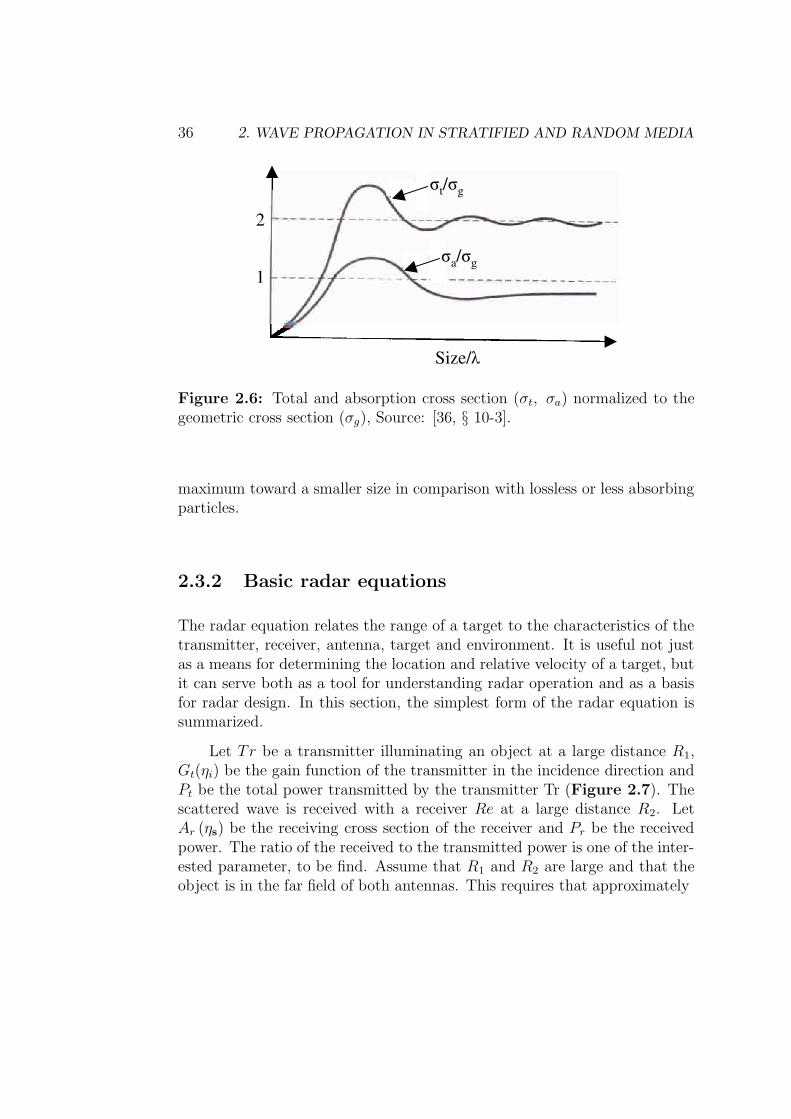
36 2. WAVE PROPAGATION IN STRATIFIED AND RANDOM MEDIA
σt/σg
σa/σg
Size/λ
2
1
Figure 2.6: Total and absorption cross section (σt, σa) normalized to thegeometric cross section (σg), Source: [36, § 10-3].
maximum toward a smaller size in comparison with lossless or less absorbingparticles.
2.3.2 Basic radar equations
The radar equation relates the range of a target to the characteristics of thetransmitter, receiver, antenna, target and environment. It is useful not justas a means for determining the location and relative velocity of a target, butit can serve both as a tool for understanding radar operation and as a basisfor radar design. In this section, the simplest form of the radar equation issummarized.
Let Tr be a transmitter illuminating an object at a large distance R1,Gt(ηi) be the gain function of the transmitter in the incidence direction andPt be the total power transmitted by the transmitter Tr (Figure 2.7). Thescattered wave is received with a receiver Re at a large distance R2. LetAr (ηs) be the receiving cross section of the receiver and Pr be the receivedpower. The ratio of the received to the transmitted power is one of the inter-ested parameter, to be find. Assume that R1 and R2 are large and that theobject is in the far field of both antennas. This requires that approximately
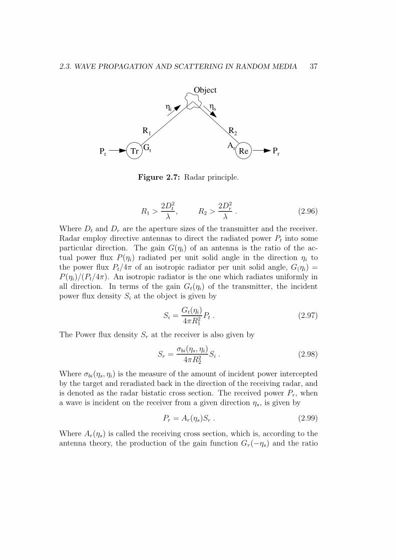
2.3. WAVE PROPAGATION AND SCATTERING IN RANDOM MEDIA 37
Tr RePt Pr
R1 R2
ηi ηs
Object
ArGt
Figure 2.7: Radar principle.
R1 >2D2
t
λ, R2 >
2D2r
λ. (2.96)
Where Dt and Dr are the aperture sizes of the transmitter and the receiver.Radar employ directive antennas to direct the radiated power Pt into someparticular direction. The gain G(ηi) of an antenna is the ratio of the ac-tual power flux P (ηi) radiated per unit solid angle in the direction ηi tothe power flux Pt/4π of an isotropic radiator per unit solid angle, G(ηi) =P (ηi)/(Pt/4π). An isotropic radiator is the one which radiates uniformly inall direction. In terms of the gain Gt(ηi) of the transmitter, the incidentpower flux density Si at the object is given by
Si =Gt(ηi)
4πR21
Pt . (2.97)
The Power flux density Sr at the receiver is also given by
Sr =σbi(ηs, ηi)
4πR22
Si . (2.98)
Where σbi(ηs, ηi) is the measure of the amount of incident power interceptedby the target and reradiated back in the direction of the receiving radar, andis denoted as the radar bistatic cross section. The received power Pr, whena wave is incident on the receiver from a given direction ηs, is given by
Pr = Ar(ηs)Sr . (2.99)
Where Ar(ηs) is called the receiving cross section, which is, according to theantenna theory, the production of the gain function Gr(−ηs) and the ratio
38 2. WAVE PROPAGATION IN STRATIFIED AND RANDOM MEDIA
λ2/4π [36, § 10-2]
Ar(ηs) =λ2
4πGr(−ηs) . (2.100)
Combining the equations from (2.97) to (2.100) gives the ratio of the receivedto the transmitted power
Pr
Pt
=λ2Gt(ηi)Gr(−ηs)σbi(ηs, ηi)
(4π)3R21R
22
. (2.101)
This is the bistatic radar equation. For monostatic radar, which used thesame antenna as a transmitter and receiver (i.e. ηs = −ηi and R1 = R2 = R),the ratio of the received to the transmitted power will be
Pr
Pt
=λ2(Gr(ηi))
2σb(−ηi, ηi)
(4π)3R4. (2.102)
Equation (2.101) and (2.102) give the received power in terms of antennagains, the distance, the cross section, wavelength and transmitted power.This is only applicable in the far field. It is also required that the receivingantenna has to be matched to the incoming wave in polarization and im-pedance. If there is a mismatch, (2.101) and (2.102) must be multiplied bythe so called mismatch factor, which is less than unity. In addition, both thetransmitter and the receiver must be in the far zone of the object.
2.3.3 Approximation of average scattered power
The last two sections demonstrates the characteristics of a single scattererand its scattering and absorption cross sections as well as the basic radarequation. By means of the single scattering approximation and first ordermultiple scattering representation, it is possible to drive important formulasconcerning wave fluctuation, narrow and wide band pulse propagation, andparticle motion. These topics are special interest to communication andradar engineers, who have been extensively treated them in many literatures[2, 33, 34, 37]. Due to some restriction of applications, the present sectionattempts the step towards approximation of the average scattered power byrandomly distributed particles.
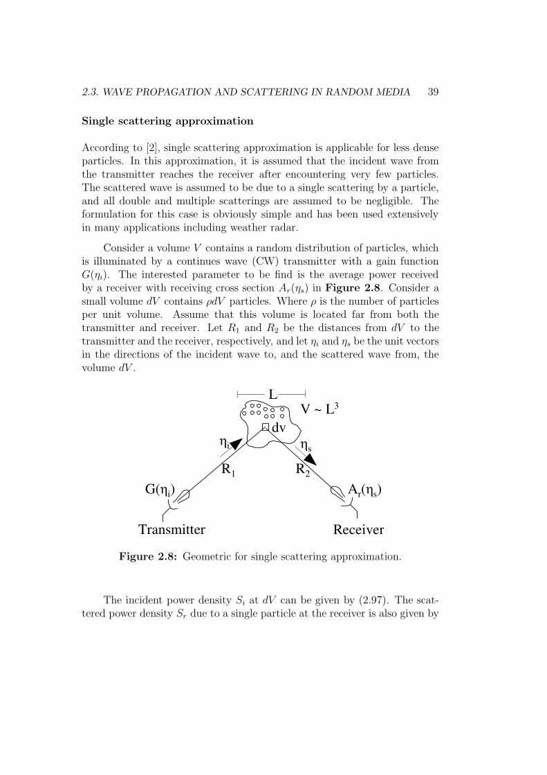
2.3. WAVE PROPAGATION AND SCATTERING IN RANDOM MEDIA 39
Single scattering approximation
According to [2], single scattering approximation is applicable for less denseparticles. In this approximation, it is assumed that the incident wave fromthe transmitter reaches the receiver after encountering very few particles.The scattered wave is assumed to be due to a single scattering by a particle,and all double and multiple scatterings are assumed to be negligible. Theformulation for this case is obviously simple and has been used extensivelyin many applications including weather radar.
Consider a volume V contains a random distribution of particles, whichis illuminated by a continues wave (CW) transmitter with a gain functionG(ηi). The interested parameter to be find is the average power receivedby a receiver with receiving cross section Ar(ηs) in Figure 2.8. Consider asmall volume dV contains ρdV particles. Where ρ is the number of particlesper unit volume. Assume that this volume is located far from both thetransmitter and receiver. Let R1 and R2 be the distances from dV to thetransmitter and the receiver, respectively, and let ηi and ηs be the unit vectorsin the directions of the incident wave to, and the scattered wave from, thevolume dV .
Transmitter
R1
ηi
R2
ηs
Receiver
G(ηi) Ar(ηs)
L
dvV ~ L3
Figure 2.8: Geometric for single scattering approximation.
The incident power density Si at dV can be given by (2.97). The scat-tered power density Sr due to a single particle at the receiver is also given by
40 2. WAVE PROPAGATION IN STRATIFIED AND RANDOM MEDIA
(2.98). Because of the randomness of the particle distribution, interferencebetween waves scattered by different particles can be neglected and merelyadd the power scattered once from all particles in dV . Thus, the total scat-tered power density Sr at the receiver due to all particles in dV is givenby
Sr =ρσbi(ηs, ηi)
4πR22
SidV . (2.103)
According to (2.99), the corresponding total received power Pr is, therefore,given by the volume integral of the received power for bistatic radar equationof a single particle
Pr
Pt
=∫
v
λ2Gt(ηi)Gt(ηs)
(4π)3R21R
22
ρσbi(ηs, ηi)dV . (2.104)
Note that equation (2.104) is applicable when the receiver is matched in bothimpedance and polarization [38, p. 4].
For a monostatic radar where the transmitter is also used as the receiver(R1 = R2 = R), the total received power Pr is given by the volume integralof the received power for monostatic radar equation of a single particle
Pr
Pt
=∫
v
λ2Gt(ηi)2ρσb
(4π)3R4dV . (2.105)
In practice, these radar equations should be modified by including im-pedance and polarization mismatch and other losses [39, Chap. 2].The validity of the single scattering approximation depends on the extentto which the incident wave encounters particles in the volume V . This maybe measured most conveniently by means of the optical distance γ or knownas attenuation coefficient. The single scattering approximation is then validwhen
γ =∫ L
0ρσtds << 1 . (2.106)
The integration is taken over a path through the volume V , and L is a lineardimension of V (Figure 2.8).
As the particle density is increased, it is no longer possible to assumethat the direct wave is identical to the incident wave, and it forced to take intoaccount attenuation due to scattering and absorption along the path. The
2.3. WAVE PROPAGATION AND SCATTERING IN RANDOM MEDIA 41
wave incident on the particle has been previously attenuated by scatteringand absorption along the scattering path, and the scattered wave too. Thisconsiders some of the multiple scattering effect, which may be expressed asfollows by the first-order multiple scattering principle.
First-order multiple scattering representation
First order multiple scattering takes into account attenuation by scatter-ing and absorption of a wave propagating along a ray path. This methodis often used in millimeter and optical wave propagation through rain, fog,smog, and snow [2].
The first order multiple scattering can be easily included by extend-ing the radar equations for the single scattering approximation, discussedin the preceding section. The incident power density Si at dV in Figure2.8 should now include attenuation term e−γ1 due to the total cross section.Where γ1 is the optical distance from the transmitter to dV and is given byγ1 =
∫ R1
0 ρσtds. The number of particles (or density) ρ(s) and the total crosssection σt(s) can be a function of the position along the path from the trans-mitter to dV . Similarly, the scattered power density Sr should be multipliedby e−γ2 . Where γ2 is also the optical distance from dV to the receiver and isgiven by γ2 =
∫ R2
0 ρσtds.
For monostatic radar (i.e. R1 = R2 = R and γ1 = γ2 = γ), the receivedpower Pr given in (2.105) can be then modified for the first-order multiplescattering case as follows
Pr
Pt
=∫
v
λ2Gt(ηi)2ρσb
(4π)3R4e−2γdV , (2.107)
where γ is given by
γ =∫ R
0ρ< σt >ds
.(2.108)
In this derivation the effects of particle size distribution is not considered.This can be easily incorporated in the (2.107) by substituting the total crosssection σt and the backscattered cross section σb with their average valuedefined in the following manner
ρ< σt > =∫ ∞
0n (D, r)σt (D)dD, (2.109)
42 2. WAVE PROPAGATION IN STRATIFIED AND RANDOM MEDIA
ρ< σb > =∫ ∞
0n (D, r)σb (D)dD (2.110)
Where n(D, r) is the number of particles per unit volume located at r havinga range of sizes between D and D+ dD and ρ is the number of particles perunit volume given by
ρ(r) =∫ ∞
0n (D, r)dD . (2.111)
Chapter 3
Automotive radar
Automotive radar senors are required to track many targets simultaneously,in range, velocity and angle to perform vehicle control. Ideally, the sensorwill have the ability to measure target angle information in elevation as wellas azimuth to allow discrimination of extended objects in the vehicle pathsuch as bridges and overpasses. Currently, this is considered to increasethe coast and complexity to a prohibitive level. In the future as sensorantennas develop, it can be expected that this requirement will be fulfilledby smart antenna solutions like two-dimensional phased arrays amongst othersolutions.
Actual automotive radar sensors represent an important class of mono-static radar system that have been the preferred antenna format for the auto-motive industry, primarily to keep the antenna aperture area to a minimumand to reduce cost. However, this is not necessarily the optimum topologyfor radar performance since it is generally dominated by transmitter noisebreakthrough rather than the noise figure as in systems with monostaticantennas.
This chapter gives mainly a short review about the measurement systemand antenna technology of an actual automotive radar sensor (or LRR2 1),on which the feasibility of theoretical results of this work will be probed.
1LRR2: Bosch second generation Automotive Long Range Radar Sensor
43
44 3. AUTOMOTIVE RADAR
3.1 Principles of distance and speed
measurements
As stated in section 2.3.2, a radar operates by transmitting electromagneticenergy towards the target and obtaining information concerning the locationand identification of the target by detecting the backscattered energy. Therange of the target is determined by measuring the time difference ∆t be-tween transmission and reception of the electromagnetic energy. If the radartransmitter and receiver are in the same casing, the target range R can bedetermined from
R =c
2∆t , (3.1)
where c is the speed of electromagnetic wave propagation in free space (see in(A.16)). For an approximated maximum detection range of an automotiveradar sensor up to 200 m (e.g. LRR2 [40]), the time difference ∆t to bemeasured is 1.33 µs.
The total angular excursion φ made by the electromagnetic wave duringits transit time ∆t to and from the targets given by φ = 4πR/λ. If thereis a relative motion between the radar and the target, the target range Rand the corresponding phase φ are continually changing. The change in Rand φ with respect to time are know as relative velocity vr and as Dopplerangular frequency wd, respectively. According to [41, § 3.1], this relationshipbetween the Doppler frequency fd = wd/2π and the relative velocity vr of atarget with respect to radar can be expressed by
fd =2
λvr . (3.2)
For an automotive radar sensor, which operates at 76.5 GHz, equation (3.2)gives a Doppler frequency of 510 Hz for a 1 m/s of relative velocity vr. Thetarget of an automotive radar sensor could be moved relative to the radarat speed of up to 250 km/h, which corresponds to a measurable Dopplerfrequency of 35.4 KHz.
Measurement accuracy
There is obviously a conflict in obtaining range accuracy and simultaneously
3.1. PRINCIPLES OF DISTANCE AND SPEED MEASUREMENTS 45
obtaining velocity accuracy with simple wave forms like pulse and continu-ous wave (CW) radars that are not modulated in the phase. In such a case,the multiplication of the standard division of errors for range and Dopplerfrequency is given by [41, § 11.3]
δTRδf =1
βτ (2S/N). (3.3)
Where
• S/N is the signal-to-noise ratio of the measurement,
• τ is the effective time duration of the signal,
• β is the effective bandwidth of the signal,
• δTR and δf are the standard division of errors for range and frequencyrespectively.
The increase in bandwidth results in better range measurements but lessaccurate in velocity measurements, and vice versa. This requires the compli-ance of the uncertainty relation, which states that the product of the effectivebandwidth β and the effective time duration τ of the signal must be graterthan or equal to π. As it is stated in the communication theory, this is oneof the main requirement for an optimum amount of information or measureddata passed through a communication channel [42, 43].
The solution to meet such requirement involves the use of waveforms,which have been modulated in phase. For example, in the case of an au-tomotive radar application, Frequency Modulated Continuous Wave radar(FMCW-radar) can perform measurements with relatively good accuracy atsignal-to-noise ratios at which measurements done by a pulse-radar may suf-fer under inaccuracy. This is due to longer illumination time of targets byFMCW-radar than pulse radar.
FMCW-radar needs in the order of ten or more milliseconds for thefrequency modulation of several hundred megahertz. The pulse radar, onthe other hand, operates with pulse duration of a few nanoseconds (< 25ns),which may lead to smaller bandwidth due to limited rise time. Measurementaccuracy of FMCW-radar system has been investigated on point target andresults have been provided in [44].
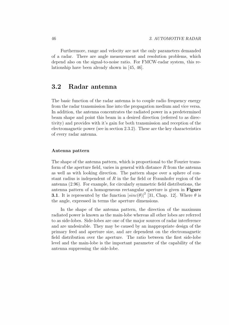
46 3. AUTOMOTIVE RADAR
Furthermore, range and velocity are not the only parameters demandedof a radar. There are angle measurement and resolution problems, whichdepend also on the signal-to-noise ratio. For FMCW-radar system, this re-lationship have been already shown in [45, 46].
3.2 Radar antenna
The basic function of the radar antenna is to couple radio frequency energyfrom the radar transmission line into the propagation medium and vice versa.In addition, the antenna concentrates the radiated power in a predeterminedbeam shape and point this beam in a desired direction (referred to as direc-tivity) and provides with it’s gain for both transmission and reception of theelectromagnetic power (see in section 2.3.2). These are the key characteristicsof every radar antenna.
Antenna pattern
The shape of the antenna pattern, which is proportional to the Fourier trans-form of the aperture field, varies in general with distance R from the antennaas well as with looking direction. The pattern shape over a sphere of con-stant radius is independent of R in the far field or Fraunhofer region of theantenna (2.96). For example, for circularly symmetric field distributions, theantenna pattern of a homogeneous rectangular aperture is given in Figure3.1. It is represented by the function |sinc(θ)|2 [31, Chap. 12]. Where θ isthe angle, expressed in terms the aperture dimensions.
In the shape of the antenna pattern, the direction of the maximumradiated power is known as the main-lobe whereas all other lobes are referredto as side-lobes. Side-lobes are one of the major sources of radar interferenceand are undesirable. They may be caused by an inappropriate design of theprimary feed and aperture size, and are dependent on the electromagneticfield distribution over the aperture. The ratio between the first side-lobelevel and the main-lobe is the important parameter of the capability of theantenna suppressing the side-lobe.
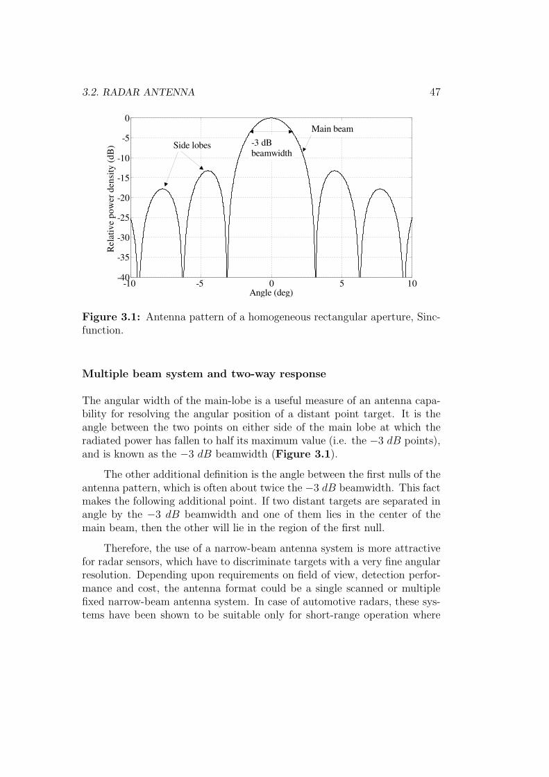
3.2. RADAR ANTENNA 47
-10 -5 0 5 10-40
-35
-30
-25
-20
-15
-10
-5
0
Angle (deg)
Rel
ativ
e po
wer
den
sity
(dB
)
Main beam
Side lobes -3 dBbeamwidth
Figure 3.1: Antenna pattern of a homogeneous rectangular aperture, Sinc-function.
Multiple beam system and two-way response
The angular width of the main-lobe is a useful measure of an antenna capa-bility for resolving the angular position of a distant point target. It is theangle between the two points on either side of the main lobe at which theradiated power has fallen to half its maximum value (i.e. the −3 dB points),and is known as the −3 dB beamwidth (Figure 3.1).
The other additional definition is the angle between the first nulls of theantenna pattern, which is often about twice the −3 dB beamwidth. This factmakes the following additional point. If two distant targets are separated inangle by the −3 dB beamwidth and one of them lies in the center of themain beam, then the other will lie in the region of the first null.
Therefore, the use of a narrow-beam antenna system is more attractivefor radar sensors, which have to discriminate targets with a very fine angularresolution. Depending upon requirements on field of view, detection perfor-mance and cost, the antenna format could be a single scanned or multiplefixed narrow-beam antenna system. In case of automotive radars, these sys-tems have been shown to be suitable only for short-range operation where
48 3. AUTOMOTIVE RADAR
road curvature is not significant. But, operation at longer range leads tothe possibility of missed target or incorrect target lane identification aroundbends [1, 47].
-80
-70
-60
-50
-40
-30
-15 -10 -5 0 5 10 15
Angle (deg)
Nor
mal
ized
am
plitu
de (d
B)
Beam 1 Beam 2 Beam 3 Beam 4
Figure 3.2: Normalized two-way antenna pattern of the LRR2-Prototype.
Radar targets and clutter use the antenna’s two-way pattern, which isthe square of the one-way pattern if the antenna is said to be reciprocal (i.e.the transmit and the receive pattern of the antenna are usually identical)[48, § 4.2.5]. For radar targets and clutter, the −3 dB beamwidth becomesthen the −6 dB beamwidth, and side lobs are lowered to double their one-way dB value. Figure 3.2 shows, for example, the normalized two-wayantenna patterns of multiple fixed beam system, implemented by the LRR2-Prototype. It has an angular coverage of about ±8 deg in the azimuth plane.This multi-beam antenna pattern is used to determine the exact angle ofa target by applying the so called Monopulse systems, which performs anamplitude and a phase comparison between adjacent beams [41, 45, 46]. Theangular coverage is needed to track the targets in the lanes ahead in order to
3.2. RADAR ANTENNA 49
anticipate vehicles cutting in front of the driver and in order to distinguishbetween targets that pose a threat and those that do not.
Radar antenna types
The antenna is a key element for automotive radar senors. Requirements,like packaging volume, cost and performance of the sensor are decisive factorson the choice of antenna. The following antenna solutions have been usedover the years:
• mechanically scanned parabolic reflector antennas
• quasi-optic lens antennas illuminated by patch radiators
• horn antennas
• static and mechanically scanned planar arrays
• mechanically scanned twist polarization cassegrain reflector and
• frequency scanned antennas
Static planar array provide a low volume antenna whereas mechanicalscanning increases the sensor volume due to the scanning mechanism assem-bly and possibly due to antenna component movement. Quasi-optic solu-tions, by virtue of the depth associated to with the focal point, also producea sensor with increased volume. However, it has gained acceptance with theautomotive manufacturer due to the possibility that the radar sensor can bemounted without special radome. For example, the lens antenna discussedbelow.
Lens antenna
Lens antennas, likewise reflector antennas, work on the principle of the the-ory of geometrical optics [32, 49]. The most important parameter in lensantenna design is the refractive index of the lens materials that may beused for the construction of the lens. It can be classified as solid dielectrics,metallic delay dielectrics, path length dielectrics, metal-plate dielectrics and
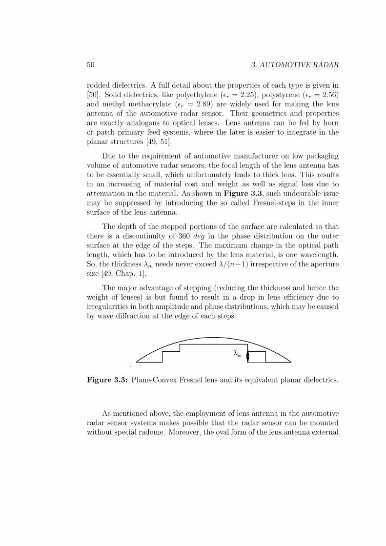
50 3. AUTOMOTIVE RADAR
rodded dielectrics. A full detail about the properties of each type is given in[50]. Solid dielectrics, like polyethylene (εr = 2.25), polystyrene (εr = 2.56)and methyl methacrylate (εr = 2.89) are widely used for making the lensantenna of the automotive radar sensor. Their geometrics and propertiesare exactly analogous to optical lenses. Lens antenna can be fed by hornor patch primary feed systems, where the later is easier to integrate in theplanar structures [49, 51].
Due to the requirement of automotive manufacturer on low packagingvolume of automotive radar sensors, the focal length of the lens antenna hasto be essentially small, which unfortunately leads to thick lens. This resultsin an increasing of material cost and weight as well as signal loss due toattenuation in the material. As shown in Figure 3.3, such undesirable issuemay be suppressed by introducing the so called Fresnel-steps in the innersurface of the lens antenna.
The depth of the stepped portions of the surface are calculated so thatthere is a discontinuity of 360 deg in the phase distribution on the outersurface at the edge of the steps. The maximum change in the optical pathlength, which has to be introduced by the lens material, is one wavelength.So, the thickness λm needs never exceed λ/(n−1) irrespective of the aperturesize [49, Chap. 1].
The major advantage of stepping (reducing the thickness and hence theweight of lenses) is but found to result in a drop in lens efficiency due toirregularities in both amplitude and phase distributions, which may be causedby wave diffraction at the edge of each steps.
λm
Figure 3.3: Plane-Convex Fresnel lens and its equivalent planar dielectrics.
As mentioned above, the employment of lens antenna in the automotiveradar sensor systems makes possible that the radar sensor can be mountedwithout special radome. Moreover, the oval form of the lens antenna external
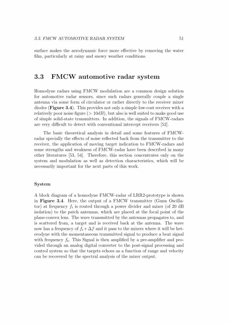
3.3. FMCW AUTOMOTIVE RADAR SYSTEM 51
surface makes the aerodynamic force more effective by removing the waterfilm, particularly at rainy and snowy weather conditions.
3.3 FMCW automotive radar system
Homodyne radars using FMCW modulation are a common design solutionfor automotive radar sensors, since such radars generally couple a singleantenna via some form of circulator or rather directly to the receiver mixerdiodes (Figure 3.4). This provides not only a simple low-cost receiver with arelatively poor noise figure (> 10dB), but also is well suited to make good useof simple solid-state transmitters. In addition, the signals of FMCW-radarsare very difficult to detect with conventional intercept receivers [52].
The basic theoretical analysis in detail and some features of FMCW-radar specially the effects of noise reflected back from the transmitter to thereceiver, the application of moving target indication to FMCW-radars andsome strengths and weakness of FMCW-radar have been described in manyother literatures [53, 54]. Therefore, this section concentrates only on thesystem and modulation as well as detection characteristics, which will benecessarily important for the next parts of this work.
System
A block diagram of a homodyne FMCW-radar of LRR2-prototype is shownin Figure 3.4. Here, the output of a FMCW transmitter (Gunn Oscilla-tor) at frequency ft is routed through a power divider and mixer (of 20 dBisolation) to the patch antennas, which are placed at the focal point of theplane-convex lens. The wave transmitted by the antennas propagates to, andis scattered from, a target and is received back at the antenna. The wavenow has a frequency of ft +∆f and it pass to the mixers where it will be het-erodyne with the momentaneous transmitted signal to produce a beat signalwith frequency fb. This Signal is then amplified by a pre-amplifier and pro-vided through an analog digital converter to the post-signal processing andcontrol system so that the targets echoes as a function of range and velocitycan be recovered by the spectral analysis of the mixer output.
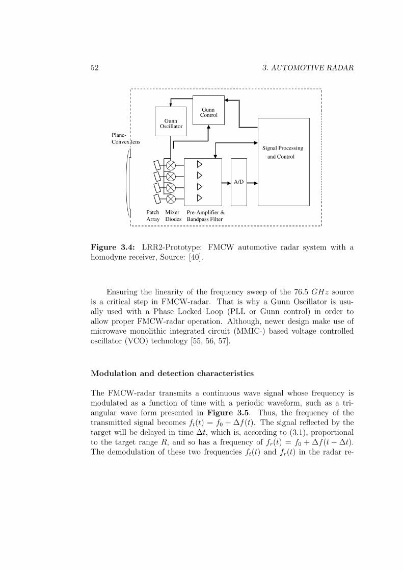
52 3. AUTOMOTIVE RADAR
Signal Processing
and Control
GunnControl
A/D
GunnOscillator
Pre-Amplifier & Bandpass Filter
Mixer Diodes
Patch Array
Plane-Convex lens
Figure 3.4: LRR2-Prototype: FMCW automotive radar system with ahomodyne receiver, Source: [40].
Ensuring the linearity of the frequency sweep of the 76.5 GHz sourceis a critical step in FMCW-radar. That is why a Gunn Oscillator is usu-ally used with a Phase Locked Loop (PLL or Gunn control) in order toallow proper FMCW-radar operation. Although, newer design make use ofmicrowave monolithic integrated circuit (MMIC-) based voltage controlledoscillator (VCO) technology [55, 56, 57].
Modulation and detection characteristics
The FMCW-radar transmits a continuous wave signal whose frequency ismodulated as a function of time with a periodic waveform, such as a tri-angular wave form presented in Figure 3.5. Thus, the frequency of thetransmitted signal becomes ft(t) = f0 + ∆f(t). The signal reflected by thetarget will be delayed in time ∆t, which is, according to (3.1), proportionalto the target range R, and so has a frequency of fr(t) = f0 + ∆f(t− ∆t).The demodulation of these two frequencies ft(t) and fr(t) in the radar re-
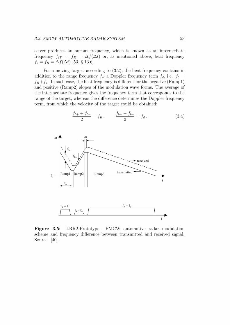
3.3. FMCW AUTOMOTIVE RADAR SYSTEM 53
ceiver produces an output frequency, which is known as an intermediatefrequency fIF = fR = ∆f(∆t) or, as mentioned above, beat frequencyfb = fR = ∆f(∆t) [53, § 13.6].
For a moving target, according to (3.2), the beat frequency contains inaddition to the range frequency fR a Doppler frequency term fd, i.e. fb =fR+fd. In such case, the beat frequency is different for the negative (Ramp1)and positive (Ramp2) slopes of the modulation wave forms. The average ofthe intermediate frequency gives the frequency term that corresponds to therange of the target, whereas the difference determines the Doppler frequencyterm, from which the velocity of the target could be obtained:
fb+ + fb−2
= fR,fb+ − fb−
2= fd . (3.4)
t
Ramp3
∆f
f0
fR + fd
t
tm
∆t
Ramp2Ramp1
fR + fdfR - fd
transmitted
received
fb-
fb+
Figure 3.5: LRR2-Prototype: FMCW automotive radar modulationscheme and frequency difference between transmitted and received signal,Source: [40].
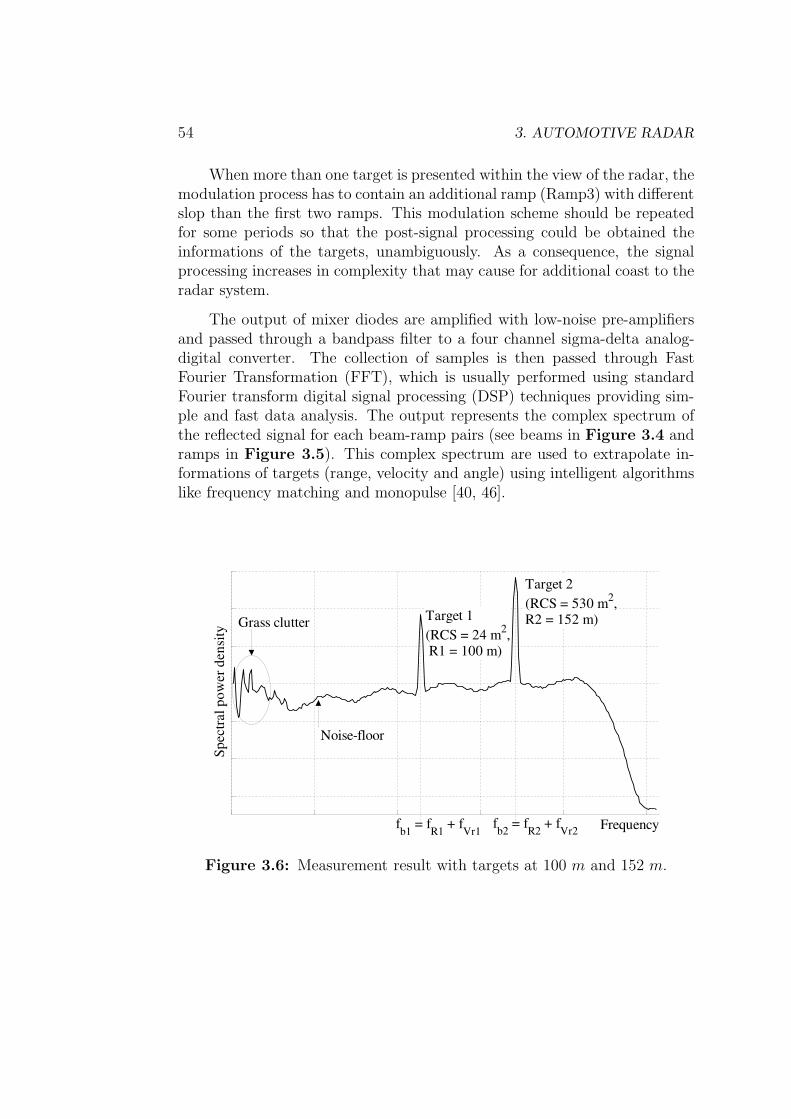
54 3. AUTOMOTIVE RADAR
When more than one target is presented within the view of the radar, themodulation process has to contain an additional ramp (Ramp3) with differentslop than the first two ramps. This modulation scheme should be repeatedfor some periods so that the post-signal processing could be obtained theinformations of the targets, unambiguously. As a consequence, the signalprocessing increases in complexity that may cause for additional coast to theradar system.
The output of mixer diodes are amplified with low-noise pre-amplifiersand passed through a bandpass filter to a four channel sigma-delta analog-digital converter. The collection of samples is then passed through FastFourier Transformation (FFT), which is usually performed using standardFourier transform digital signal processing (DSP) techniques providing sim-ple and fast data analysis. The output represents the complex spectrum ofthe reflected signal for each beam-ramp pairs (see beams in Figure 3.4 andramps in Figure 3.5). This complex spectrum are used to extrapolate in-formations of targets (range, velocity and angle) using intelligent algorithmslike frequency matching and monopulse [40, 46].
Frequency
Spec
tral
pow
er d
ensi
ty
Target 2 (RCS = 530 m2,R2 = 152 m) Target 1
(RCS = 24 m2, R1 = 100 m)
fb1 = fR1 + fVr1fb2 = fR2 + fVr2
Noise-floor
Grass clutter
Figure 3.6: Measurement result with targets at 100 m and 152 m.
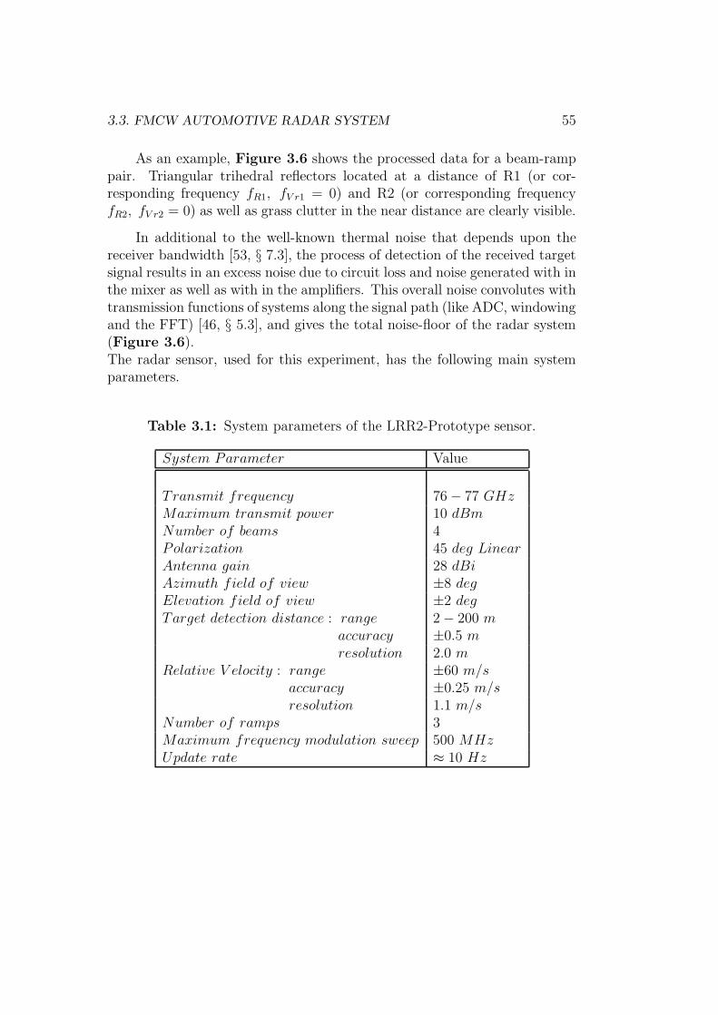
3.3. FMCW AUTOMOTIVE RADAR SYSTEM 55
As an example, Figure 3.6 shows the processed data for a beam-ramppair. Triangular trihedral reflectors located at a distance of R1 (or cor-responding frequency fR1, fV r1 = 0) and R2 (or corresponding frequencyfR2, fV r2 = 0) as well as grass clutter in the near distance are clearly visible.
In additional to the well-known thermal noise that depends upon thereceiver bandwidth [53, § 7.3], the process of detection of the received targetsignal results in an excess noise due to circuit loss and noise generated with inthe mixer as well as with in the amplifiers. This overall noise convolutes withtransmission functions of systems along the signal path (like ADC, windowingand the FFT) [46, § 5.3], and gives the total noise-floor of the radar system(Figure 3.6).The radar sensor, used for this experiment, has the following main systemparameters.
Table 3.1: System parameters of the LRR2-Prototype sensor.
System Parameter Value
Transmit frequency 76 − 77 GHzMaximum transmit power 10 dBmNumber of beams 4Polarization 45 deg LinearAntenna gain 28 dBiAzimuth field of view ±8 degElevation field of view ±2 degTarget detection distance : range 2 − 200 m
accuracy ±0.5 mresolution 2.0 m
Relative V elocity : range ±60 m/saccuracy ±0.25 m/sresolution 1.1 m/s
Number of ramps 3Maximum frequency modulation sweep 500 MHzUpdate rate ≈ 10 Hz
Chapter 4
Effects of water film onmillimeter-wave radar
The wetness of an antenna surface or its covering radome can mainly becaused by adverse weather conditions such as rain, snow and weather underfreezing temperature. Considerable works have been done in the past onanalysis and measurements of the effects of water film on micro-wave prop-agation [58, 59, 60]. These studies have obtained quantitative data, whichdemonstrates that the water film generally affects electromagnetic wave prop-agation at micro-wave frequencies and results in a considerable loss. Basedon that, it is here proceeding to work out in detail these effects on millimeterwave signals using the theoretical fundament given in § 2.2.
To obtain a quantitative result on the effects of water film on the per-formance of automotive radars, extensive measurements of reflectivity andtransmissivity at 76.5 GHz have been made in the laboratory. Furthermore,application oriented experiments have been also performed using an automo-tive radar sensor, discussed in Chapter 3.
This chapter demonstrates essentially the potential of millimeter-waveradar sensor for identification of the effects of water film on the detectioncharacteristics. This may be used to control the performance of automotiveradar sensor systems within the bounds of possibilities.
56
4.1. THEORETICAL ANALYSIS 57
4.1 Theoretical analysis
The performance of automotive radar sensors is a significant consideration inthe choice of placement, with sensor height affecting both multipath perfor-mance and ancillary issues such as aperture obscuration by dirt, water andice or slush. However, the front grille area has been the traditional placementarea for actual automotive radar sensors and it is mounted at the height ofabout 35 cm above the road [40, 46].
Depending up on the requirement of the vehicle manufacturer, the radarmust be housed with a radome or not. But, the presence of a radome canaffect the gain, beamwidth, side-lobe level, and the pointing direction (bore-sight), as well as change the voltage-standing wave ratio (VSWR) and theantenna noise temperature [41, § 7.9]. Therefore, it should be designed prop-erly, to distort the antenna pattern as little as possible.
In designing millimeter-wave radar sensors for use in ACC and sub-sequent systems, there is a requirement for data detailing degradation ofperformance caused by propagation through (and reflection by) water filmon the surface of antenna or radome. For that matter, the presence of awater film on the surface of radome has been represented by the followingwave propagation model, in order to observe its effect on the millimeter-wavepropagation.
4.1.1 Wave propagation model
The formation of water on the radome surface, and then in the propagationpath of radar signal, can be represented by the multi-layer wave propagationmodel (Figure 4.1). The radome-water film system is enclosed by air. Itis principally the extension of the theory to stratified media that containabsorbing element, i.e. water. Thus, the effects of water film on millimeter-wave radar performance can be examined by revise the equations given in §2.2 for this model and by matching physical parameters.
As it is clearly remarked in § 2.2, the linear equation systems (2.44)to (2.47) for the perpendicular polarized wave (or TE-Wave) and (2.60) to(2.63) for the parallel polarized wave or (TM-Wave) can be modified for anynumber of multi-layer media. The way, how these modifications can be done
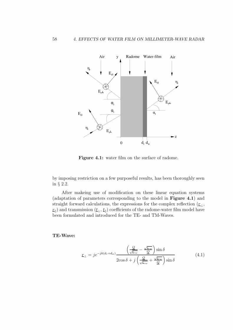
58 4. EFFECTS OF WATER FILM ON MILLIMETER-WAVE RADAR
Ei||
Water-film
Er||
Ei
dr dw
Radome
z
Et||
y
αr
αt
Er
Et
0
ηi
ηr
ηt
αi
Air Air
Figure 4.1: water film on the surface of radome.
by imposing restriction on a few purposeful results, has been thoroughly seenin § 2.2.
After makeing use of modification on these linear equation systems(adaptation of parameters corresponding to the model in Figure 4.1) andstraight forward calculations, the expressions for the complex reflection (r⊥,r‖) and transmission (t⊥, t‖) coefficients of the radome-water film model havebeen formulated and introduced for the TE- and TM-Waves.
TE-Wave:
r⊥ = je−jk(dr+dw)
(
Q√
εrw
−√
εrw
Q
)
sin δ
2cos δ + j(
Q√
εrw
+√
εrw
Q
)
sin δ(4.1)
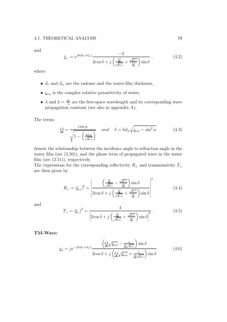
4.1. THEORETICAL ANALYSIS 59
and
t⊥ = ejk(dr+dw) −2
2cos δ + j(
Q√
εrw
+√
εrw
Q
)
sin δ, (4.2)
where
• dr and dw are the radome and the water-film thickness,
• εrw is the complex relative permittivity of water,
• λ and k = 2πλ
are the free-space wavelength and its corresponding wavepropagation constant (see also in appendix A).
The terms
Q =cosα
√
1 −(
sinα√εrw
)
and δ = kdw
√
εrw − sin2 α (4.3)
denote the relationship between the incidence angle to refraction angle in thewater film (see (2.50)), and the phase term of propagated wave in the waterfilm (see (2.51)), respectively.The expressions for the corresponding reflectivity R⊥ and transmissivity T⊥are then given by
R⊥ = |r⊥|2 =
∣
∣
∣
∣
∣
∣
∣
∣
(
Q√
εrw
−√
εrw
Q
)
sin δ
2cos δ + j(
Q√
εrw
+√
εrw
Q
)
sin δ
∣
∣
∣
∣
∣
∣
∣
∣
2
(4.4)
and
T⊥ = |t⊥|2 =4
∣
∣
∣
∣
2cos δ + j(
Q√
εrw
+√
εrw
Q
)
sin δ
∣
∣
∣
∣
2 . (4.5)
TM-Wave:
r‖ = je−jk(dr+dw)
(
Q√εrw − 1
Q√
εrw
)
sin δ
2cos δ + j(
Q√εrw + 1
Q√
εrw
)
sin δ(4.6)
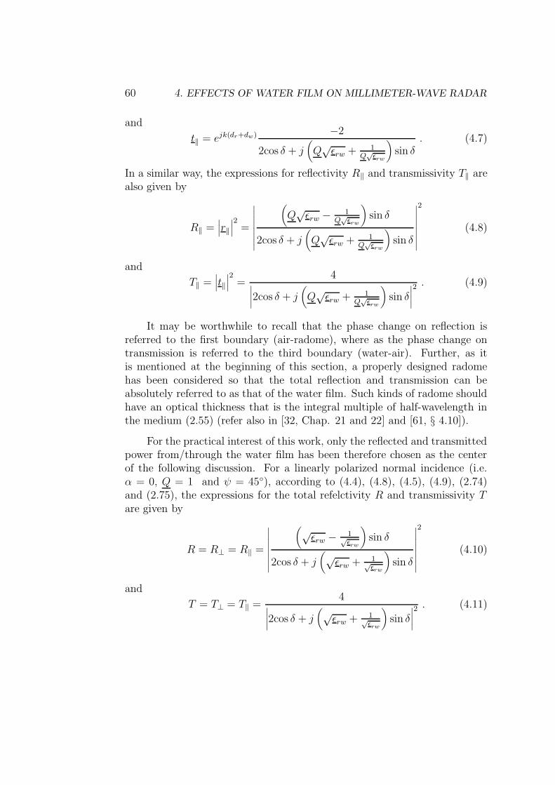
60 4. EFFECTS OF WATER FILM ON MILLIMETER-WAVE RADAR
and
t‖ = ejk(dr+dw) −2
2cos δ + j(
Q√εrw + 1
Q√
εrw
)
sin δ. (4.7)
In a similar way, the expressions for reflectivity R‖ and transmissivity T‖ arealso given by
R‖ =∣
∣
∣r‖∣
∣
∣
2=
∣
∣
∣
∣
∣
∣
∣
∣
(
Q√εrw − 1
Q√
εrw
)
sin δ
2cos δ + j(
Q√εrw + 1
Q√
εrw
)
sin δ
∣
∣
∣
∣
∣
∣
∣
∣
2
(4.8)
and
T‖ =∣
∣
∣t‖∣
∣
∣
2=
4∣
∣
∣
∣
2cos δ + j(
Q√εrw + 1
Q√
εrw
)
sin δ
∣
∣
∣
∣
2 . (4.9)
It may be worthwhile to recall that the phase change on reflection isreferred to the first boundary (air-radome), where as the phase change ontransmission is referred to the third boundary (water-air). Further, as itis mentioned at the beginning of this section, a properly designed radomehas been considered so that the total reflection and transmission can beabsolutely referred to as that of the water film. Such kinds of radome shouldhave an optical thickness that is the integral multiple of half-wavelength inthe medium (2.55) (refer also in [32, Chap. 21 and 22] and [61, § 4.10]).
For the practical interest of this work, only the reflected and transmittedpower from/through the water film has been therefore chosen as the centerof the following discussion. For a linearly polarized normal incidence (i.e.α = 0, Q = 1 and ψ = 45), according to (4.4), (4.8), (4.5), (4.9), (2.74)and (2.75), the expressions for the total refelctivity R and transmissivity Tare given by
R = R⊥ = R‖ =
∣
∣
∣
∣
∣
∣
∣
∣
(√εrw − 1√
εrw
)
sin δ
2cos δ + j(√
εrw + 1√εrw
)
sin δ
∣
∣
∣
∣
∣
∣
∣
∣
2
(4.10)
and
T = T⊥ = T‖ =4
∣
∣
∣
∣
2cos δ + j(√
εrw + 1√εrw
)
sin δ
∣
∣
∣
∣
2 . (4.11)

4.1. THEORETICAL ANALYSIS 61
0.1 0.2 0.3 0.4 0.5 0.6 0.7 0.8 0.9 1-10
-8
-6
-4
-2
0
Water-film thickness, dw (mm)
Ref
lekt
ivity
(dB
)
f = 24 GHz
f = 76 GHz
f = 140 GHz
drise
Figure 4.2: Reflectivity from water film at 20 C.
Where ψ is the polarization angle of the incidence wave.
Equations (4.1) - (4.11) allow computations of quantities that character-ize reflection and transmission by water film of known electrical propertiesand of prescribed thickness. Figures 4.2 and 4.3 show the dependence ofreflectivity and transmissivity on the thickness of the water film at 20 C forthree frequencies, which are used for automotive radar sensors.
According to equations (2.10) and (A.23), the intensity of the electro-magnetic wave propagated along the water film is attenuated by the atten-uation factor of e
−4π
λκdw . In the millimeter-wave range, the imaginary part
of the complex permittivity of water ε′′ and its corresponding significantabsorption coefficient κ decreases gradually with increasing frequency (Fig-ure 2.2). Thus, the absorption of electromagnetic wave in the water filmincreases with frequency as well as with water-film thickness.
As shown in Figure 4.2, the reflectivity is seen to reduce the amplitudeof the successive maxima and to give rise to a displacement of the max-ima in the direction of smaller thickness. At the penetration or so calledskin-depth, where the wave attenuates to the value 36.8% of its original am-plitude, absorption of water film is so large that the thickness at which thereis appreciable transmission is well below a quarter wavelength in meadim,i.e. dw ≤ λ/4
√εrw . Consequently, the reflectivity will approach to a con-
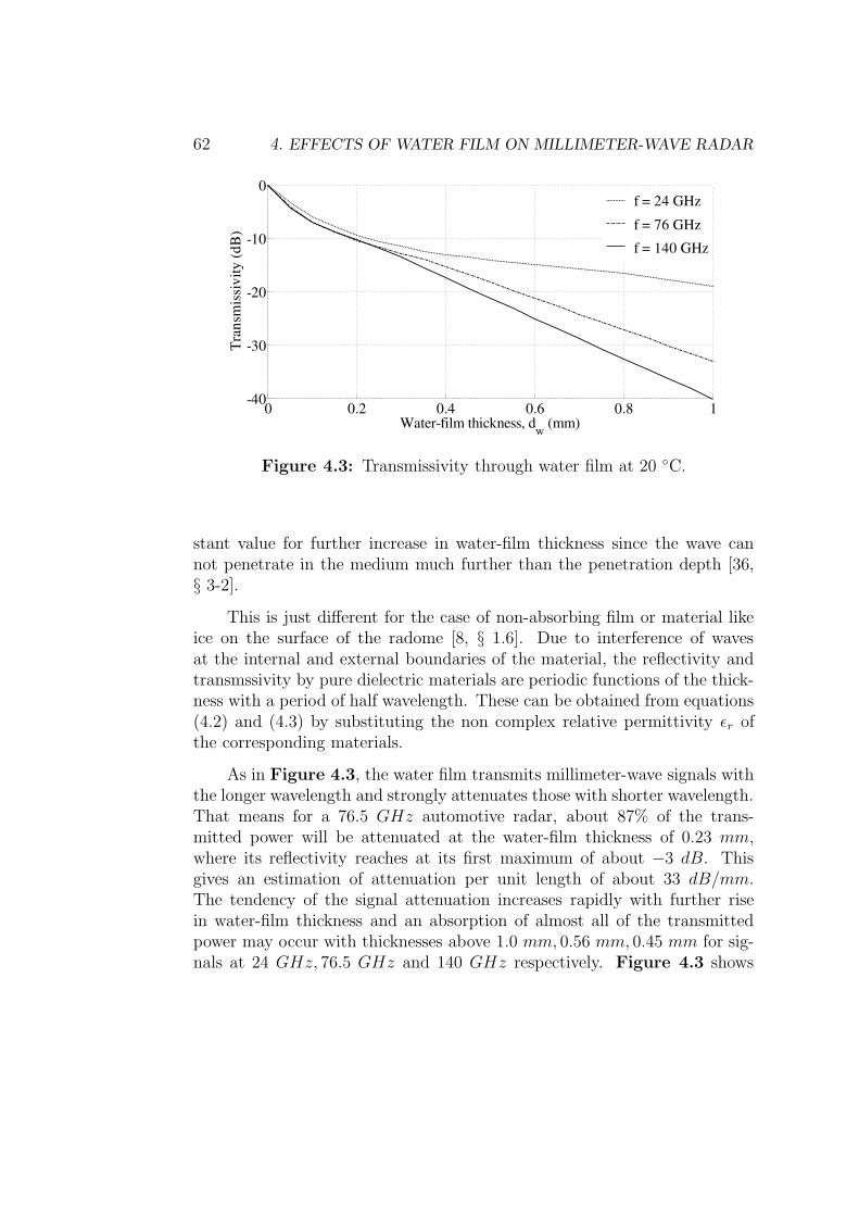
62 4. EFFECTS OF WATER FILM ON MILLIMETER-WAVE RADAR
0 0.2 0.4 0.6 0.8 1-40
-30
-20
-10
0
Water-film thickness, dw (mm)
Tra
nsm
issi
vity
(dB
)
f = 24 GHz
f = 76 GHz
f = 140 GHz
Figure 4.3: Transmissivity through water film at 20 C.
stant value for further increase in water-film thickness since the wave cannot penetrate in the medium much further than the penetration depth [36,§ 3-2].
This is just different for the case of non-absorbing film or material likeice on the surface of the radome [8, § 1.6]. Due to interference of wavesat the internal and external boundaries of the material, the reflectivity andtransmssivity by pure dielectric materials are periodic functions of the thick-ness with a period of half wavelength. These can be obtained from equations(4.2) and (4.3) by substituting the non complex relative permittivity εr ofthe corresponding materials.
As in Figure 4.3, the water film transmits millimeter-wave signals withthe longer wavelength and strongly attenuates those with shorter wavelength.That means for a 76.5 GHz automotive radar, about 87% of the trans-mitted power will be attenuated at the water-film thickness of 0.23 mm,where its reflectivity reaches at its first maximum of about −3 dB. Thisgives an estimation of attenuation per unit length of about 33 dB/mm.The tendency of the signal attenuation increases rapidly with further risein water-film thickness and an absorption of almost all of the transmittedpower may occur with thicknesses above 1.0 mm, 0.56 mm, 0.45 mm for sig-nals at 24 GHz, 76.5 GHz and 140 GHz respectively. Figure 4.3 shows
4.1. THEORETICAL ANALYSIS 63
also that the attenuation increases with frequencies in which the loss tangentof water ascends (Figure 2.2). It proceeds then with gradual growth forfrequencies where the loss tangent starts to decrease.
4.1.2 Derivation of the water-film indicator
The water film with thicknesses mentioned above can be easily formed onthe surface of millimeter-wave antenna in adverse weather conditions andmay degrade millimeter-wave radar performance. Specially automotive radarsensors, which are widely used as comfort and collision mitigation productsin the automotive market, needs to detect automatically such performancedegradation. This requires the usage of an indicator, which shall be deducedfrom the physical phenomena of the causes. For this purpose, the relationshipbetween the effects of water film has been examined as follows.
As it is seen in equations (4.10) and (4.11), the reflectivity and trans-missivity of the incident wave on the radome-water film system are relatedover their denominators. Further, according to Figure 4.2, the reflectivityfrom the water film is large enough to be measured, if it propagates back toand received by the antenna as well as if the radar system includes an ap-propriate measurement system. Therefore, it shall be meaningful to expressthe transmissivity T as a function of reflectivity R, in order to detect theamount of the signal absorbed by the water film.
Substituting the denominator of (4.11) by (4.10) gives the transmissivityT in terms of the reflectivity R, the complex relative permittivity εrw of thewater film and phase term δ = kdwεrw of the propagated wave in the waterfilm
T =4
∣
∣
∣
∣
(
1√εrw
−√εrw
)
sin δ∣
∣
∣
∣
2R, for dw < drise , (4.12)
where drise is the so called rise thickness at which the reflections coefficientr reaches about 90% of its maximum amplitude [62, Chap. 18]. Accordingto (4.10), it can be approximated by drise ≈ 0.57 λ
4√
εrw
(Figure 4.2).
Because of an ambiguous value of the reflectivity for the water-film thick-ness greater than drise, equation (4.12) could not provide a correct value forthe transmissivity. Its application is therefore limited for a water-film thick-
64 4. EFFECTS OF WATER FILM ON MILLIMETER-WAVE RADAR
ness up to drise and it represents exactly the theoretical relationship betweenthe transmissivity and reflectivity. The complex relative permittivity εrw
can be calculated from equations (2.11) and (2.12) for a given frequency andtemperature respectively (see also Figure 2.2 and Figure 2.3).
With equation (4.12), it is achieved to present the definition ofan unmeasurable effect of water film on millimeter-wave radar sig-nal (transmissivity) with the corresponding measurable effect (re-flectivity). This can be applied for calculating the amount of powerpropagated through the water film so that the actual detectionrange as well as the actual detection capacity of millimeter-waveradar sensors can be approximated automatically. It is purposefulparticularly for controlling performance of automotive radar sen-sors, which have to operate by all weather scenario, also includingadverse weather conditions.
Further, the water-film thickness formed on the antenna surface canbe approximated from the measured reflectivity using equations (4.10) and(4.3). Equation (4.12) is plotted in Figure 4.4 for a 76.5 GHz millimeter-wave radar incorporation with the water-film thickness and the maximumdetection range of an 76.5 GHz automotive radar sensor. The maximumdetection range of the radar and its relationship with transmissivity will bediscussed in the next section.
Generally speaking, Figure 4.4 demonstrates the outcome of the abovetheoretical analysis, how the attenuation of an electromagnetic wave propa-gated through the water film can be determined for the radar that is designedto detect or measure the corresponding reflectivity.
4.1.3 Relationship between the water-film effects andthe radar maximum detection range
Before starting to discuss measurements, it will be helpful for understandingto review the fundamental relationship between the normalized maximumdetection range of the radar and reflectivity from the water film. This re-lationship can be obtained from the monostatic radar equation (2.102) andequation (4.12) that shows relationship between the reflectivity and trans-missivity.
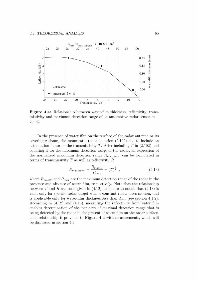
4.1. THEORETICAL ANALYSIS 65
0-10 -12 -14-16 -18-20-22-24-26
-7
-6
-5
-4
-3
Transmissivity (dB)
Ref
lect
ivity
(dB
) R
max / R
max, standard (%), RCS = 3 m2
22 25 28 32 36 40 45 50 56 100
Wat
er-f
ilm th
ickn
ess
(mm
)
calculated
measured, δ = 1%
0.23
0.13
0.10
0.08
0.06
Figure 4.4: Relationship between water-film thickness, reflectivity, trans-missivity and maximum detection range of an automotive radar sensor at20 C.
In the presence of water film on the surface of the radar antenna or itscovering radome, the monostatic radar equation (2.102) has to include anattenuation factor or the transmissivity T . After including T in (2.102) andequating it for the maximum detection range of the radar, an expression ofthe normalized maximum detection range Rmax,norm can be formulated interms of transmissivity T as well as reflectivity R
Rmax,norm =RmaxW
Rmax
= (T )1
4 , (4.13)
where RmaxW and Rmax are the maximum detection range of the radar in thepresence and absence of water film, respectively. Note that the relationshipbetween T and R has been given in (4.12). It is also to notice that (4.13) isvalid only for specific radar target with a constant radar cross section, andis applicable only for water-film thickness less than drise (see section 4.1.2).According to (4.12) and (4.13), measuring the reflectivity from water filmenables determination of the per cent of maximal detection range that isbeing detected by the radar in the present of water film on the radar surface.This relationship is provided to Figure 4.4 with measurements, which willbe discussed in section 4.3.
66 4. EFFECTS OF WATER FILM ON MILLIMETER-WAVE RADAR
4.2 Experimental investigations
The effects of films, including water film, on the electromagnetic wave propa-gation have been experimentally investigated to a great extent using differentscientific methods [25, 63]. For that matter, this work is only interested onan automatic identification of the effects of water film on detection perfor-mance of automotive radar sensors. Before attempting to measure effects ofwater film with automotive radar system, this section describes even so aless complex and an appropriate lab measuring system, validate theoreticaldiscussed before.
In section 4.3, an application oriented measurement technique will bethen followed and illustrated using an automotive radar sensor, to corrobo-rate the technical possibilities of a millimeter-wave radar to monitor its ownperformance.
4.2.1 Measurement system
Equipment
A Vector Network Analyzer (VNA1) has been used for the measurement ofeffects of water film on millimeter-wave propagation. It operates at the micro-wave and millimeter-wave region using E-band (60 GHz - 90 GHz) reflexion-transmission module 2 with an out put power of approximately 6 dBm. Itsbasic capability is to measure the S-Parameters of an Radio Frequency (RF)or micro wave device with sensitivity up to −70 dB and display the result inthe frequency domain. Measurements are acquired through IEEE 8-488 busby an analogue acquisition board placed in a personal computer. Reference[64] gives an account detailed of the VNA.
Measurement Procedure
Horn antennas are widely used as a standard in antenna measurement due totheir large gain and superior overall performance to other types of antennas.
1Vector Network Analyzer 37369A from Anritsu23740A-X Transmission/Reflection millimeter wave module
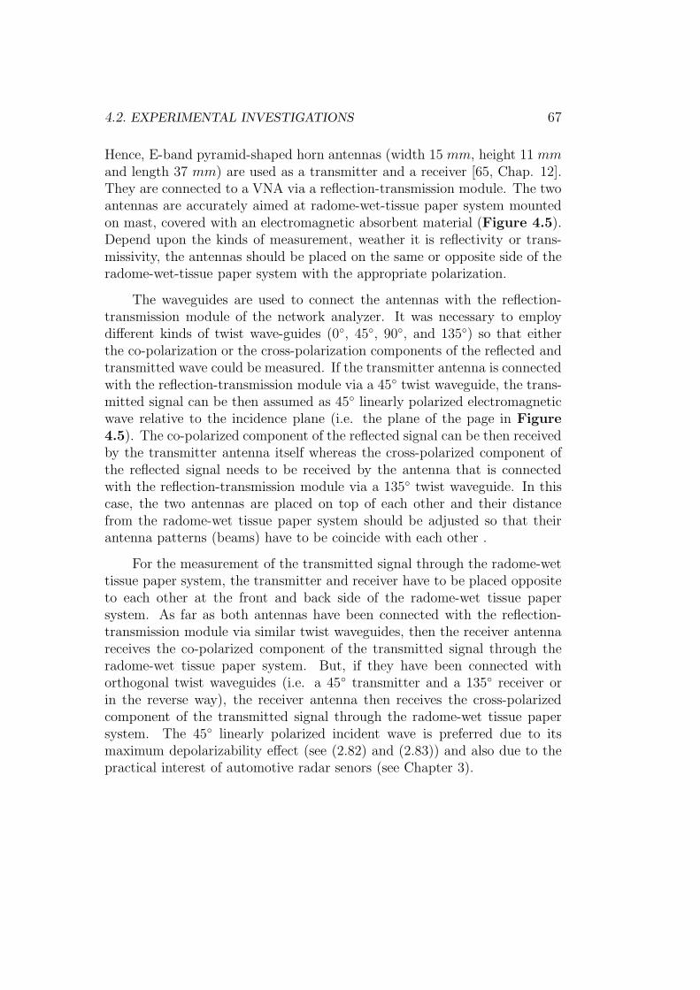
4.2. EXPERIMENTAL INVESTIGATIONS 67
Hence, E-band pyramid-shaped horn antennas (width 15 mm, height 11 mmand length 37 mm) are used as a transmitter and a receiver [65, Chap. 12].They are connected to a VNA via a reflection-transmission module. The twoantennas are accurately aimed at radome-wet-tissue paper system mountedon mast, covered with an electromagnetic absorbent material (Figure 4.5).Depend upon the kinds of measurement, weather it is reflectivity or trans-missivity, the antennas should be placed on the same or opposite side of theradome-wet-tissue paper system with the appropriate polarization.
The waveguides are used to connect the antennas with the reflection-transmission module of the network analyzer. It was necessary to employdifferent kinds of twist wave-guides (0, 45, 90, and 135) so that eitherthe co-polarization or the cross-polarization components of the reflected andtransmitted wave could be measured. If the transmitter antenna is connectedwith the reflection-transmission module via a 45 twist waveguide, the trans-mitted signal can be then assumed as 45 linearly polarized electromagneticwave relative to the incidence plane (i.e. the plane of the page in Figure4.5). The co-polarized component of the reflected signal can be then receivedby the transmitter antenna itself whereas the cross-polarized component ofthe reflected signal needs to be received by the antenna that is connectedwith the reflection-transmission module via a 135 twist waveguide. In thiscase, the two antennas are placed on top of each other and their distancefrom the radome-wet tissue paper system should be adjusted so that theirantenna patterns (beams) have to be coincide with each other .
For the measurement of the transmitted signal through the radome-wettissue paper system, the transmitter and receiver have to be placed oppositeto each other at the front and back side of the radome-wet tissue papersystem. As far as both antennas have been connected with the reflection-transmission module via similar twist waveguides, then the receiver antennareceives the co-polarized component of the transmitted signal through theradome-wet tissue paper system. But, if they have been connected withorthogonal twist waveguides (i.e. a 45 transmitter and a 135 receiver orin the reverse way), the receiver antenna then receives the cross-polarizedcomponent of the transmitted signal through the radome-wet tissue papersystem. The 45 linearly polarized incident wave is preferred due to itsmaximum depolarizability effect (see (2.82) and (2.83)) and also due to thepractical interest of automotive radar senors (see Chapter 3).
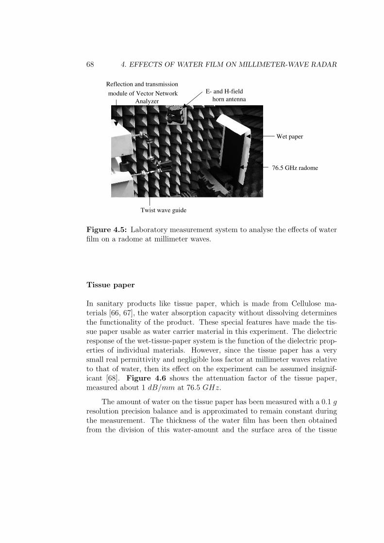
68 4. EFFECTS OF WATER FILM ON MILLIMETER-WAVE RADAR
Twist wave guide
E- and H-field horn antenna
76.5 GHz radome
Wet paper
Reflection and transmissionmodule of Vector Network
Analyzer
Figure 4.5: Laboratory measurement system to analyse the effects of waterfilm on a radome at millimeter waves.
Tissue paper
In sanitary products like tissue paper, which is made from Cellulose ma-terials [66, 67], the water absorption capacity without dissolving determinesthe functionality of the product. These special features have made the tis-sue paper usable as water carrier material in this experiment. The dielectricresponse of the wet-tissue-paper system is the function of the dielectric prop-erties of individual materials. However, since the tissue paper has a verysmall real permittivity and negligible loss factor at millimeter waves relativeto that of water, then its effect on the experiment can be assumed insignif-icant [68]. Figure 4.6 shows the attenuation factor of the tissue paper,measured about 1 dB/mm at 76.5 GHz.
The amount of water on the tissue paper has been measured with a 0.1 gresolution precision balance and is approximated to remain constant duringthe measurement. The thickness of the water film has been then obtainedfrom the division of this water-amount and the surface area of the tissue
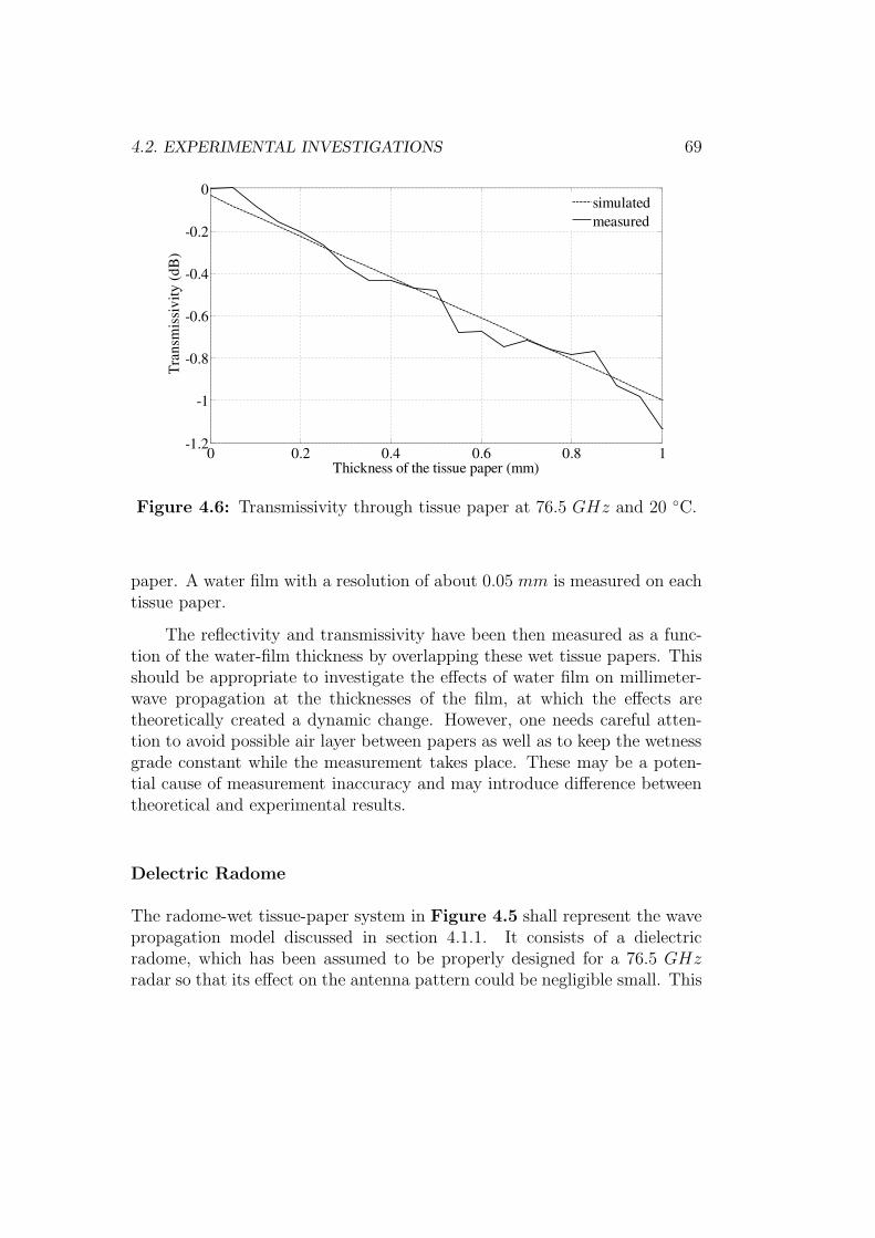
4.2. EXPERIMENTAL INVESTIGATIONS 69
0 0.2 0.4 0.6 0.8 1-1.2
-1
-0.8
-0.6
-0.4
-0.2
0
Thickness of the tissue paper (mm)
Tra
nsm
issi
vity
(dB
)
simulatedmeasured
Figure 4.6: Transmissivity through tissue paper at 76.5 GHz and 20 C.
paper. A water film with a resolution of about 0.05 mm is measured on eachtissue paper.
The reflectivity and transmissivity have been then measured as a func-tion of the water-film thickness by overlapping these wet tissue papers. Thisshould be appropriate to investigate the effects of water film on millimeter-wave propagation at the thicknesses of the film, at which the effects aretheoretically created a dynamic change. However, one needs careful atten-tion to avoid possible air layer between papers as well as to keep the wetnessgrade constant while the measurement takes place. These may be a poten-tial cause of measurement inaccuracy and may introduce difference betweentheoretical and experimental results.
Delectric Radome
The radome-wet tissue-paper system in Figure 4.5 shall represent the wavepropagation model discussed in section 4.1.1. It consists of a dielectricradome, which has been assumed to be properly designed for a 76.5 GHzradar so that its effect on the antenna pattern could be negligible small. This
70 4. EFFECTS OF WATER FILM ON MILLIMETER-WAVE RADAR
60 65 70 75 80 85 90-40.0
-26.0
-20.0
-14.0
Frequency (GHz)
Ref
lect
ivity
(dB
) dr = λ /2n ≈ 3.5 mm
f ≈ 3 GHz
Figure 4.7: Reflectivity of the radome-tissue-paper system versus frequency.
has been proofed by performing measurements on the utilized radome that ismade up of a polystyrene material (index of refraction = 1.6 and transmissionloss = 0.2 dB).
Figure 4.7 shows the reflectivity, measured on the radom-tissue-papersystem. It is almost a periodic function of the thickness of radom-tissue-paper system dr = λ/2n ≈ 3.5 mm. Where n is the combined index of therefraction of the radome-tissu paper system. Since the measurement has beenperformed in a laboratory, where the room could not be absolutely isolatedwith proper absorber materials, there are an undefined interference on mea-surements. This has been made notice on the Figure 4.7 by overlapping a3 GHz periodic signal on the measurement curve. Furthermore, Figure 4.7shows that the radome-tissue-paper system lets signal better transmitted at80 GHz than at the expected frequency, 76.5 GHz.
Calibration
The VNA is calibrated in the E-band frequency range by using the standardcalibration kit [64]. The calibration plane is transported to the measurementplane to which the measured reflection and transmission coefficient must bereferred. Then, a measurement has been taken with radome-tissue-papersystem shown in Figure 4.5. This value has been set up in the VNA as
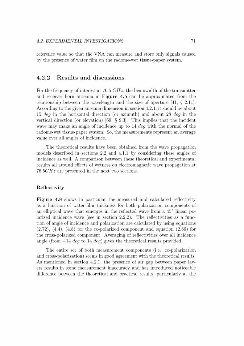
4.2. EXPERIMENTAL INVESTIGATIONS 71
reference value so that the VNA can measure and store only signals causedby the presence of water film on the radome-wet tissue-paper system.
4.2.2 Results and discussions
For the frequency of interest at 76.5 GHz, the beamwidth of the transmitterand receiver horn antenna in Figure 4.5 can be approximated from therelationship between the wavelength and the size of aperture [41, § 2.11].According to the given antenna dimension in section 4.2.1, it should be about15 deg in the horizontal direction (or azimuth) and about 28 deg in thevertical direction (or elevation) [69, § 9.3]. This implies that the incidentwave may make an angle of incidence up to 14 deg with the normal of theradome-wet tissue-paper system. So, the measurements represent an averagevalue over all angles of incidence.
The theoretical results have been obtained from the wave propagationmodels described in sections 2.2 and 4.1.1 by considering these angles ofincidence as well. A comparison between these theoretical and experimentalresults all around effects of wetness on electromagnetic wave propagation at76.5GHz are presented in the next two sections.
Reflectivity
Figure 4.8 shows in particular the measured and calculated reflectivityas a function of water-film thickness for both polarization components ofan elliptical wave that emerges in the reflected wave from a 45 linear po-larized incidence wave (see in section 2.2.2). The reflectivities as a func-tion of angle of incidence and polarization are calculated by using equations(2.72), (4.4), (4.8) for the co-polarized component and equation (2.86) forthe cross-polarized component. Averaging of reflectivities over all incidenceangle (from −14 deg to 14 deg) gives the theoretical results provided.
The entire set of both measurement components (i.e. co-polarizationand cross-polarization) seems in good agreement with the theoretical results.As mentioned in section 4.2.1, the presence of air gap between paper lay-ers results in some measurement inaccuracy and has introduced noticeabledifference between the theoretical and practical results, particularly at the
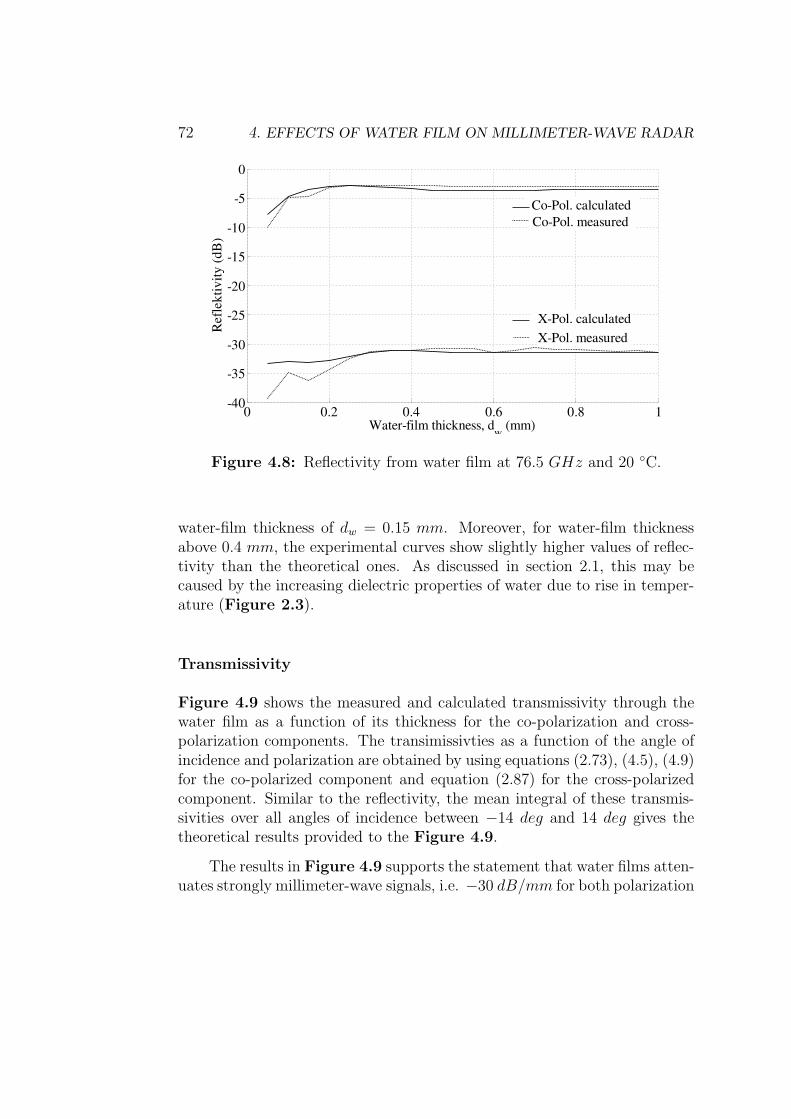
72 4. EFFECTS OF WATER FILM ON MILLIMETER-WAVE RADAR
0 0.2 0.4 0.6 0.8 1-40
-35
-30
-25
-20
-15
-10
-5
0
Water-film thickness, dw (mm)
Ref
lekt
ivity
(dB
) Co-Pol. calculated Co-Pol. measured
X-Pol. measured X-Pol. calculated
Figure 4.8: Reflectivity from water film at 76.5 GHz and 20 C.
water-film thickness of dw = 0.15 mm. Moreover, for water-film thicknessabove 0.4 mm, the experimental curves show slightly higher values of reflec-tivity than the theoretical ones. As discussed in section 2.1, this may becaused by the increasing dielectric properties of water due to rise in temper-ature (Figure 2.3).
Transmissivity
Figure 4.9 shows the measured and calculated transmissivity through thewater film as a function of its thickness for the co-polarization and cross-polarization components. The transimissivties as a function of the angle ofincidence and polarization are obtained by using equations (2.73), (4.5), (4.9)for the co-polarized component and equation (2.87) for the cross-polarizedcomponent. Similar to the reflectivity, the mean integral of these transmis-sivities over all angles of incidence between −14 deg and 14 deg gives thetheoretical results provided to the Figure 4.9.
The results in Figure 4.9 supports the statement that water films atten-uates strongly millimeter-wave signals, i.e. −30 dB/mm for both polarization
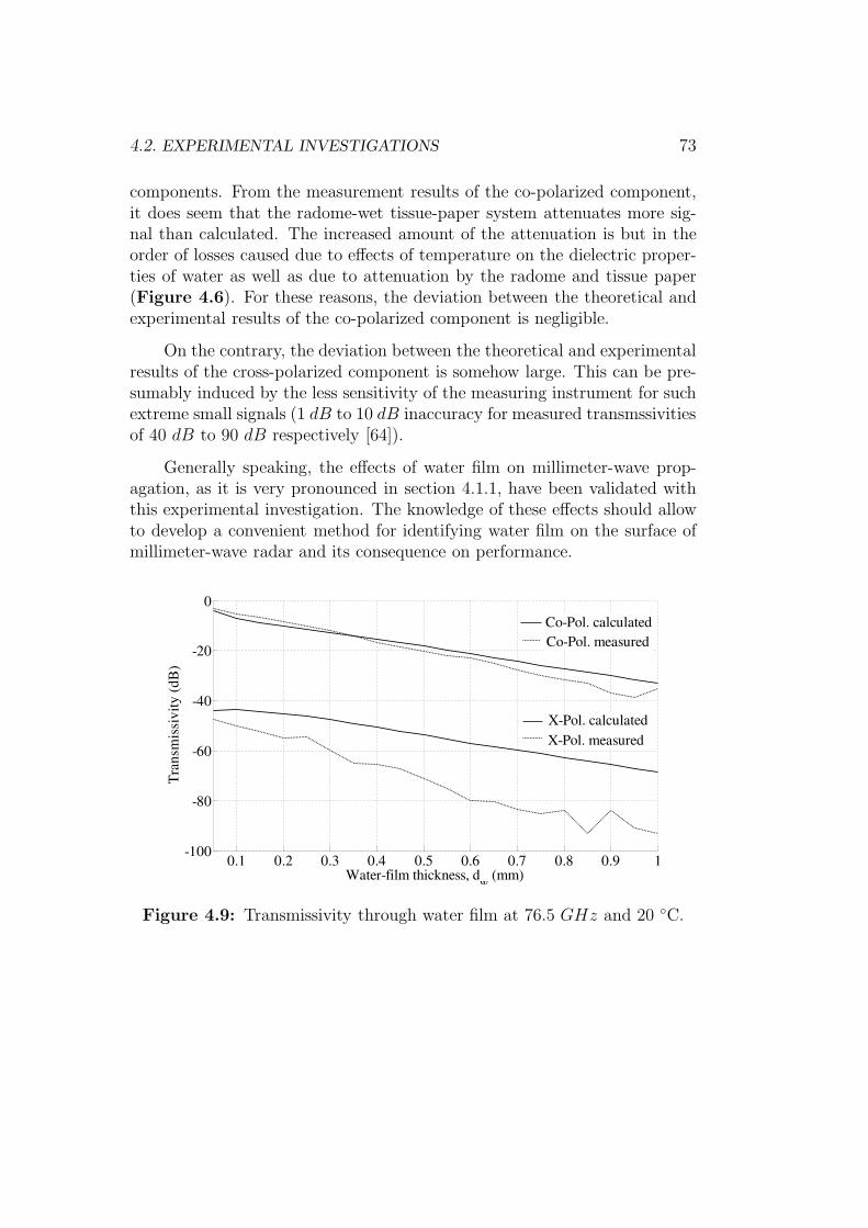
4.2. EXPERIMENTAL INVESTIGATIONS 73
components. From the measurement results of the co-polarized component,it does seem that the radome-wet tissue-paper system attenuates more sig-nal than calculated. The increased amount of the attenuation is but in theorder of losses caused due to effects of temperature on the dielectric proper-ties of water as well as due to attenuation by the radome and tissue paper(Figure 4.6). For these reasons, the deviation between the theoretical andexperimental results of the co-polarized component is negligible.
On the contrary, the deviation between the theoretical and experimentalresults of the cross-polarized component is somehow large. This can be pre-sumably induced by the less sensitivity of the measuring instrument for suchextreme small signals (1 dB to 10 dB inaccuracy for measured transmssivitiesof 40 dB to 90 dB respectively [64]).
Generally speaking, the effects of water film on millimeter-wave prop-agation, as it is very pronounced in section 4.1.1, have been validated withthis experimental investigation. The knowledge of these effects should allowto develop a convenient method for identifying water film on the surface ofmillimeter-wave radar and its consequence on performance.
0.1 0.2 0.3 0.4 0.5 0.6 0.7 0.8 0.9 1-100
-80
-60
-40
-20
0
Water-film thickness, dw (mm)
Tra
nsm
issi
vity
(dB
)
Co-Pol. calculated Co-Pol. measured
X-Pol. measured X-Pol. calculated
Figure 4.9: Transmissivity through water film at 76.5 GHz and 20 C.
74 4. EFFECTS OF WATER FILM ON MILLIMETER-WAVE RADAR
4.3 Investigations of water-film effects on an
LRR2 automotive radar sensor
So far the aim has been to develop an indicator for signal attenuation dueto the formation of water film on millimeter-wave radar surface or its cov-ering radome. Having done this, let proceed with analysis of the practicalexperiments performed on a real FMCW-automotive radar sensor. For thispurpose, the LRR2 radar introduced in section 4.3.1 has been employed inthe following way.
4.3.1 Measurement system
Equipment
The aim to perform an application oriented experiment has called for em-ploying the LRR2 sensor as measuring equipment for the effects of water filmand also rain in the propagation path of the radar signal. System of LRR2and its principle of operation have been briefly explained in Chapter 3 andthe main system parameters are given in Table 3.1.
The radar measures signal, which is returned from objects in the radarfield of view, and measurements are acquired using a standard computerlinked on-line to the radar-emulator system (Figure B.5). A measurementprogram, known as Vector CANape, is used and caused the computer to con-troll and setup the radar-emulator-computer interface. Signal returns fromthe radar field of view is sampled and calculated with the signal processingand controlling unit of the radar over 100 ms of a measuring cycle (Figure3.4). About 8192 spectrum and additional measured parameters like infor-mation of targets and parameter of components have been send to and storedin the computer for on-line or further off-line measurement analysis.
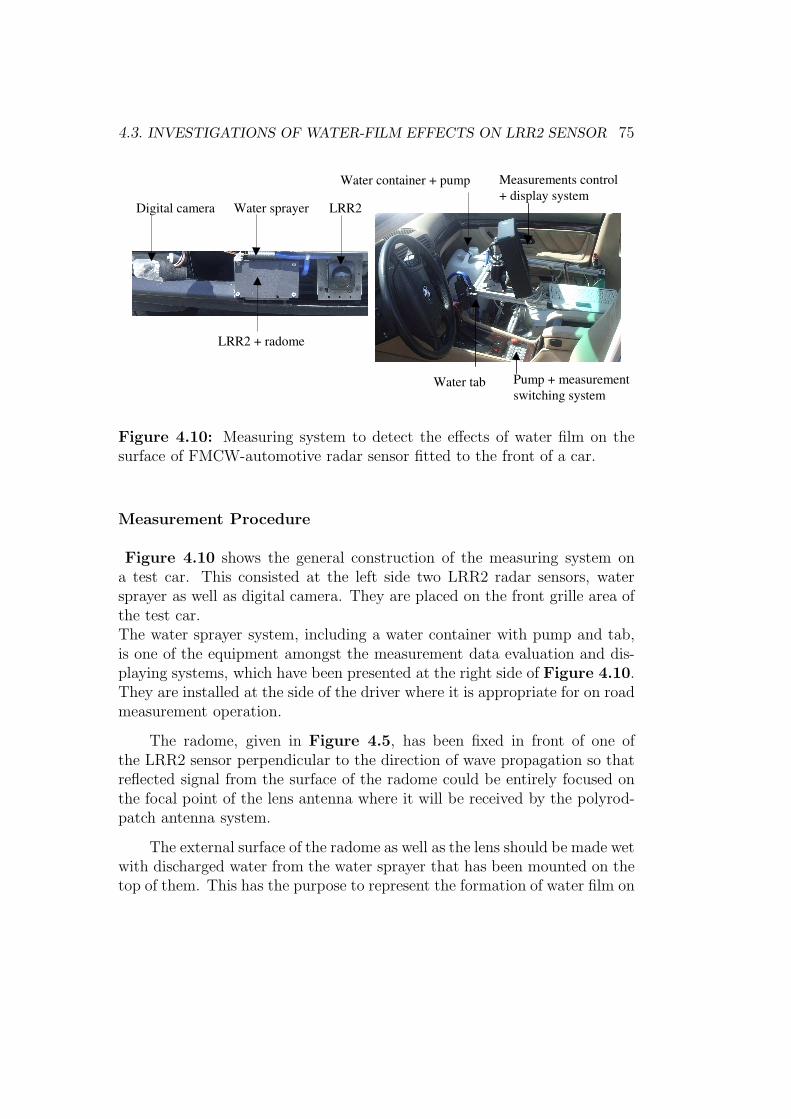
4.3. INVESTIGATIONS OF WATER-FILM EFFECTS ON LRR2 SENSOR 75
Water sprayer LRR2
LRR2 + radome
Digital camera
Water container + pump
Water tab
Measurements control+ display system
Pump + measurement switching system
Figure 4.10: Measuring system to detect the effects of water film on thesurface of FMCW-automotive radar sensor fitted to the front of a car.
Measurement Procedure
Figure 4.10 shows the general construction of the measuring system ona test car. This consisted at the left side two LRR2 radar sensors, watersprayer as well as digital camera. They are placed on the front grille area ofthe test car.The water sprayer system, including a water container with pump and tab,is one of the equipment amongst the measurement data evaluation and dis-playing systems, which have been presented at the right side of Figure 4.10.They are installed at the side of the driver where it is appropriate for on roadmeasurement operation.
The radome, given in Figure 4.5, has been fixed in front of one ofthe LRR2 sensor perpendicular to the direction of wave propagation so thatreflected signal from the surface of the radome could be entirely focused onthe focal point of the lens antenna where it will be received by the polyrod-patch antenna system.
The external surface of the radome as well as the lens should be made wetwith discharged water from the water sprayer that has been mounted on thetop of them. This has the purpose to represent the formation of water film on
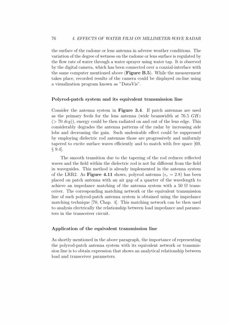
76 4. EFFECTS OF WATER FILM ON MILLIMETER-WAVE RADAR
the surface of the radome or lens antenna in adverse weather conditions. Thevariation of the degree of wetness on the radome or lens surface is regulated bythe flow rate of water through a water sprayer using water tap. It is observedby the digital camera, which has been connected over a coaxial-interface withthe same computer mentioned above (Figure B.5). While the measurementtakes place, recorded results of the camera could be displayed on-line usinga visualization program known as ”DataVis”.
Polyrod-patch system and its equivalent transmission line
Consider the antenna system in Figure 3.4. If patch antennas are usedas the primary feeds for the lens antenna (wide beamwidth at 76.5 GHz(> 70 deg)), energy could be then radiated on and out of the lens edge. Thisconsiderably degrades the antenna patterns of the radar by increasing sidelobs and decreasing the gain. Such undesirable effect could be suppressedby employing dielectric rod antennas those are progressively and uniformlytapered to excite surface waves efficiently and to match with free space [69,§ 9.4].
The smooth transition due to the tapering of the rod reduces reflectedwaves and the field within the dielectric rod is not far different from the fieldin waveguides. This method is already implemented in the antenna systemof the LRR2. As Figure 4.11 shows, polyrod antenna (εr = 2.8) has beenplaced on patch antenna with an air gap of a quarter of the wavelength toachieve an impedance matching of the antenna system with a 50 Ω trans-ceiver. The corresponding matching network or the equivalent transmissionline of such polyrod-patch antenna system is obtained using the impedancematching technique [70, Chap. 4]. This matching network can be then usedto analysis electrically the relationship between load impedance and parame-ters in the transceiver circuit.
Application of the equivalent transmission line
As shortly mentioned in the above paragraph, the importance of representingthe polyrod-patch antenna system with its equivalent network or transmis-sion line is to obtain expression that shows an analytical relationship betweenload and transceiver parameters.
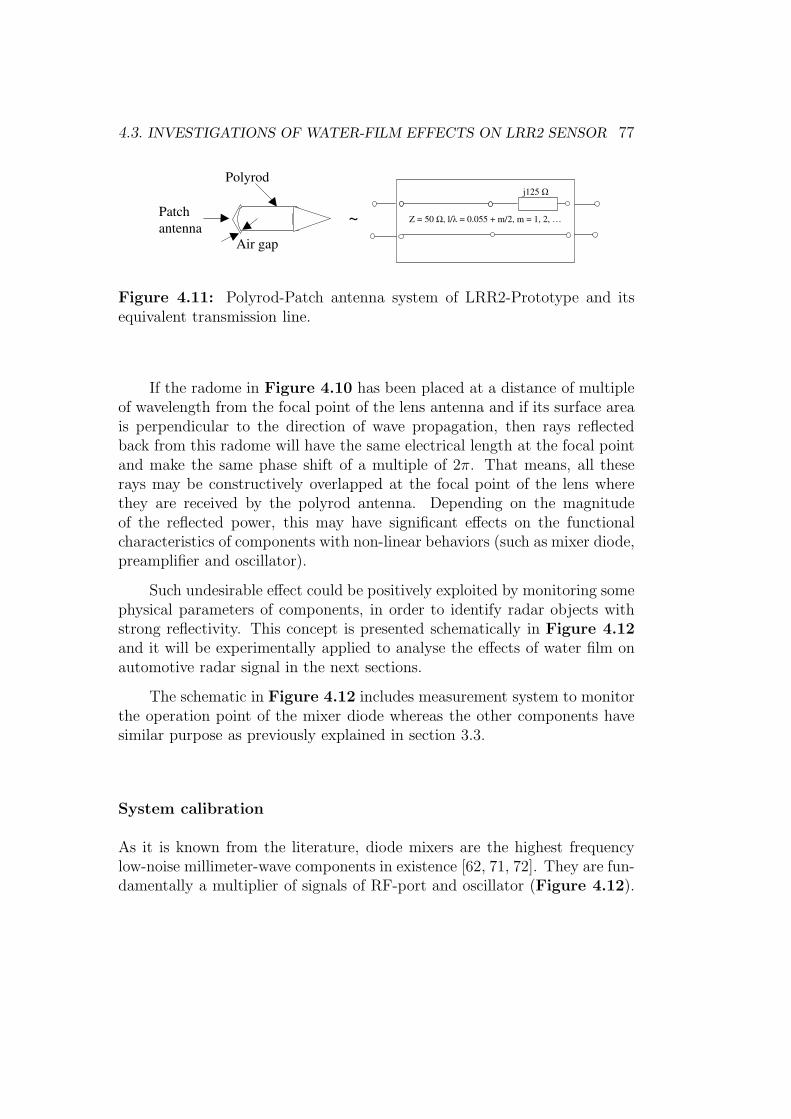
4.3. INVESTIGATIONS OF WATER-FILM EFFECTS ON LRR2 SENSOR 77
j125 Ω
Z = 50 Ω, l/λ = 0.055 + m/2, m = 1, 2, …Patch antenna
Polyrod
~Air gap
Figure 4.11: Polyrod-Patch antenna system of LRR2-Prototype and itsequivalent transmission line.
If the radome in Figure 4.10 has been placed at a distance of multipleof wavelength from the focal point of the lens antenna and if its surface areais perpendicular to the direction of wave propagation, then rays reflectedback from this radome will have the same electrical length at the focal pointand make the same phase shift of a multiple of 2π. That means, all theserays may be constructively overlapped at the focal point of the lens wherethey are received by the polyrod antenna. Depending on the magnitudeof the reflected power, this may have significant effects on the functionalcharacteristics of components with non-linear behaviors (such as mixer diode,preamplifier and oscillator).
Such undesirable effect could be positively exploited by monitoring somephysical parameters of components, in order to identify radar objects withstrong reflectivity. This concept is presented schematically in Figure 4.12and it will be experimentally applied to analyse the effects of water film onautomotive radar signal in the next sections.
The schematic in Figure 4.12 includes measurement system to monitorthe operation point of the mixer diode whereas the other components havesimilar purpose as previously explained in section 3.3.
System calibration
As it is known from the literature, diode mixers are the highest frequencylow-noise millimeter-wave components in existence [62, 71, 72]. They are fun-damentally a multiplier of signals of RF-port and oscillator (Figure 4.12).
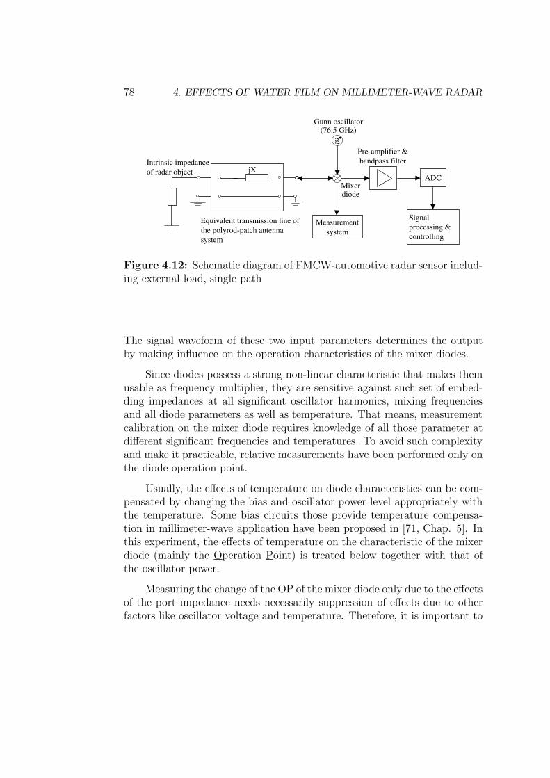
78 4. EFFECTS OF WATER FILM ON MILLIMETER-WAVE RADAR
Intrinsic impedance of radar object
Measurementsystem
ADC
Gunn oscillator(76.5 GHz)
~~~
Mixer diode
Pre-amplifier & bandpass filter
Signal processing & controlling
jX
Equivalent transmission line of the polyrod-patch antennasystem
Figure 4.12: Schematic diagram of FMCW-automotive radar sensor includ-ing external load, single path
The signal waveform of these two input parameters determines the outputby making influence on the operation characteristics of the mixer diodes.
Since diodes possess a strong non-linear characteristic that makes themusable as frequency multiplier, they are sensitive against such set of embed-ding impedances at all significant oscillator harmonics, mixing frequenciesand all diode parameters as well as temperature. That means, measurementcalibration on the mixer diode requires knowledge of all those parameter atdifferent significant frequencies and temperatures. To avoid such complexityand make it practicable, relative measurements have been performed only onthe diode-operation point.
Usually, the effects of temperature on diode characteristics can be com-pensated by changing the bias and oscillator power level appropriately withthe temperature. Some bias circuits those provide temperature compensa-tion in millimeter-wave application have been proposed in [71, Chap. 5]. Inthis experiment, the effects of temperature on the characteristic of the mixerdiode (mainly the Operation Point) is treated below together with that ofthe oscillator power.
Measuring the change of the OP of the mixer diode only due to the effectsof the port impedance needs necessarily suppression of effects due to otherfactors like oscillator voltage and temperature. Therefore, it is important to
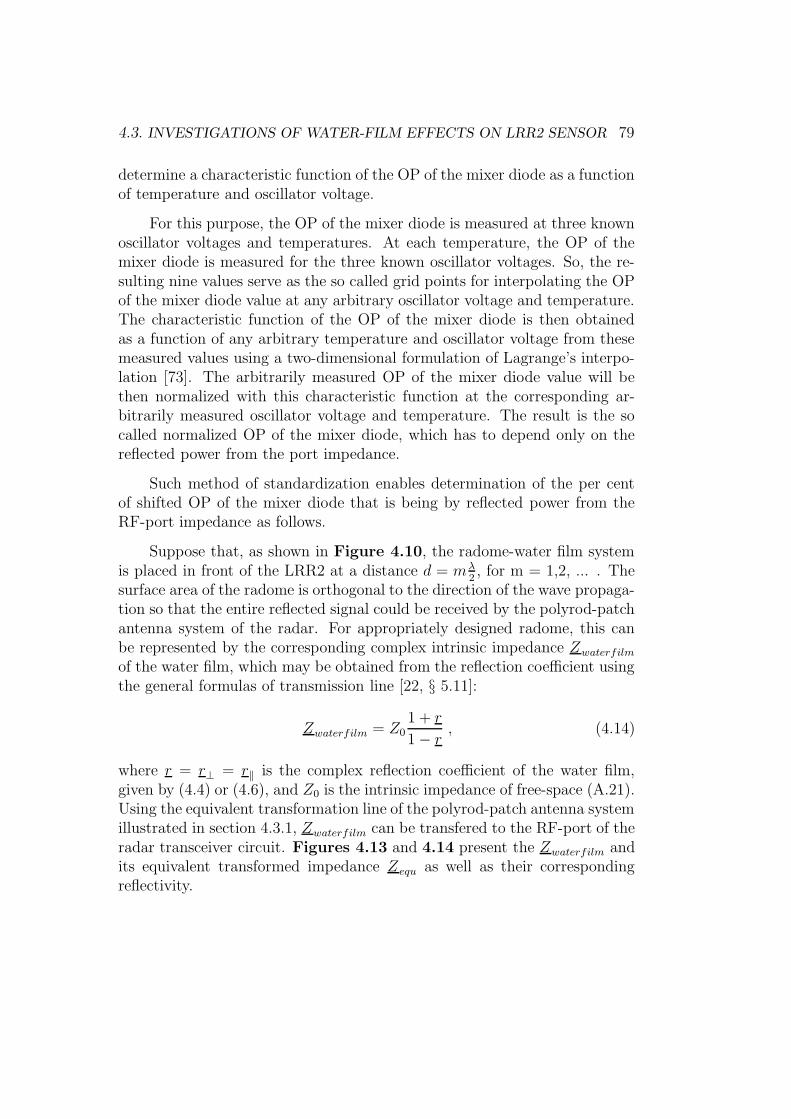
4.3. INVESTIGATIONS OF WATER-FILM EFFECTS ON LRR2 SENSOR 79
determine a characteristic function of the OP of the mixer diode as a functionof temperature and oscillator voltage.
For this purpose, the OP of the mixer diode is measured at three knownoscillator voltages and temperatures. At each temperature, the OP of themixer diode is measured for the three known oscillator voltages. So, the re-sulting nine values serve as the so called grid points for interpolating the OPof the mixer diode value at any arbitrary oscillator voltage and temperature.The characteristic function of the OP of the mixer diode is then obtainedas a function of any arbitrary temperature and oscillator voltage from thesemeasured values using a two-dimensional formulation of Lagrange’s interpo-lation [73]. The arbitrarily measured OP of the mixer diode value will bethen normalized with this characteristic function at the corresponding ar-bitrarily measured oscillator voltage and temperature. The result is the socalled normalized OP of the mixer diode, which has to depend only on thereflected power from the port impedance.
Such method of standardization enables determination of the per centof shifted OP of the mixer diode that is being by reflected power from theRF-port impedance as follows.
Suppose that, as shown in Figure 4.10, the radome-water film systemis placed in front of the LRR2 at a distance d = mλ
2, for m = 1,2, ... . The
surface area of the radome is orthogonal to the direction of the wave propaga-tion so that the entire reflected signal could be received by the polyrod-patchantenna system of the radar. For appropriately designed radome, this canbe represented by the corresponding complex intrinsic impedance Zwaterfilm
of the water film, which may be obtained from the reflection coefficient usingthe general formulas of transmission line [22, § 5.11]:
Zwaterfilm = Z01 + r
1 − r, (4.14)
where r = r⊥ = r‖ is the complex reflection coefficient of the water film,given by (4.4) or (4.6), and Z0 is the intrinsic impedance of free-space (A.21).Using the equivalent transformation line of the polyrod-patch antenna systemillustrated in section 4.3.1, Zwaterfilm can be transfered to the RF-port of theradar transceiver circuit. Figures 4.13 and 4.14 present the Zwaterfilm andits equivalent transformed impedance Zequ as well as their correspondingreflectivity.
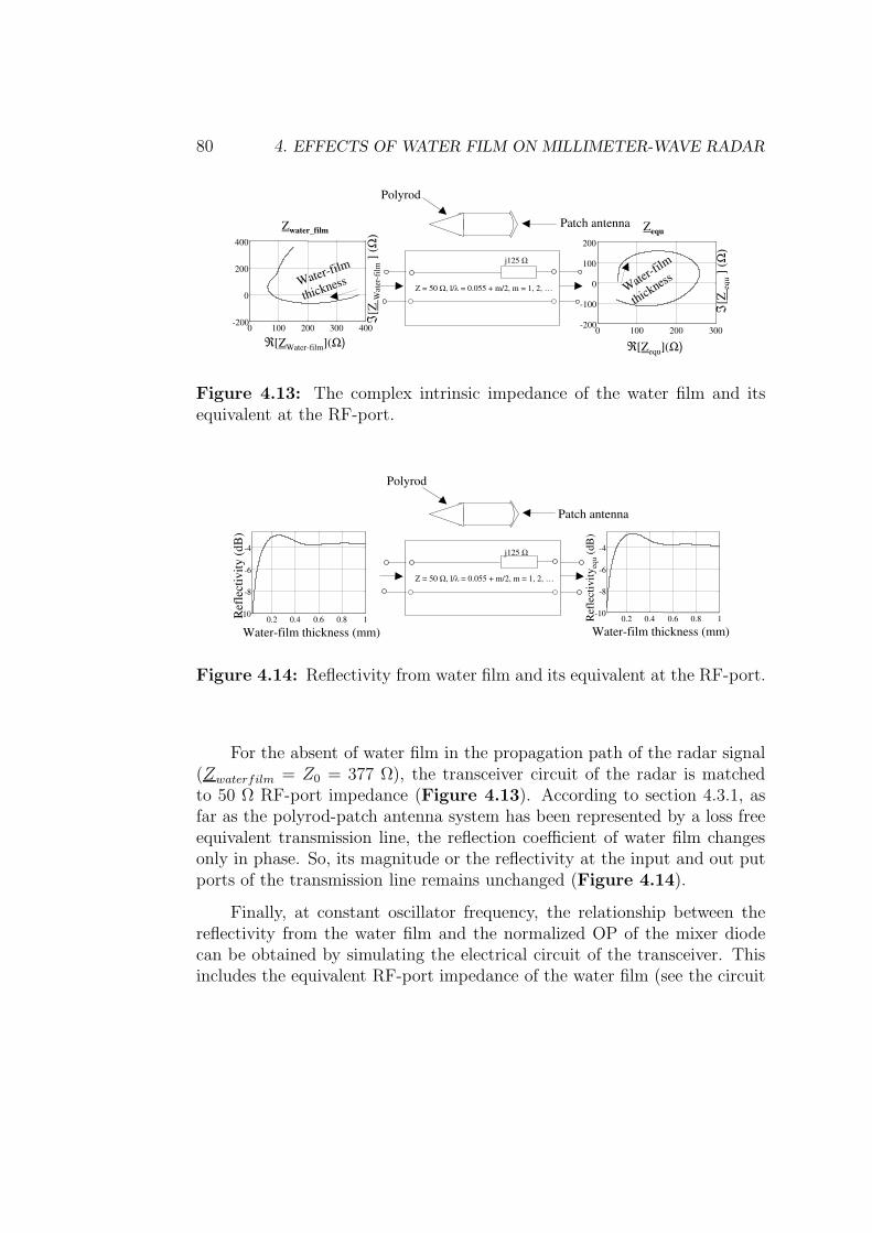
80 4. EFFECTS OF WATER FILM ON MILLIMETER-WAVE RADAR
ZequZwater_film
Wat
er-fi
lm
Thic
knes
s
Water-film
Thickness
j125 Ω
Z = 50 Ω, l/λ = 0.055 + m/2, m = 1, 2, …
Patch antenna
Polyrod
0 100 200 300 400-200
0
200
400
0 100 200 300-200
-100
0
100
200
Water-film
thickness Water-fi
lm
thickness
ℜ[ZWater-film](Ω)
ℑ[Z
Wat
er-f
ilm] (
Ω)
ℜ[Zequ](Ω)
ℑ[Z
equ
] (Ω
)
Figure 4.13: The complex intrinsic impedance of the water film and itsequivalent at the RF-port.
0.2 0.4 0.6 0.8 1-10
-8
-6
-4
Water-film thickness (mm)
Ref
lect
ivity
equ
(dB
)
0.2 0.4 0.6 0.8 1-10
-8
-6
-4
Water-film thickness (mm)
Ref
lect
ivity
(dB
)
j125 Ω
Z = 50 Ω, l/λ = 0.055 + m/2, m = 1, 2, …
Patch antenna
Polyrod
Figure 4.14: Reflectivity from water film and its equivalent at the RF-port.
For the absent of water film in the propagation path of the radar signal(Zwaterfilm = Z0 = 377 Ω), the transceiver circuit of the radar is matchedto 50 Ω RF-port impedance (Figure 4.13). According to section 4.3.1, asfar as the polyrod-patch antenna system has been represented by a loss freeequivalent transmission line, the reflection coefficient of water film changesonly in phase. So, its magnitude or the reflectivity at the input and out putports of the transmission line remains unchanged (Figure 4.14).
Finally, at constant oscillator frequency, the relationship between thereflectivity from the water film and the normalized OP of the mixer diodecan be obtained by simulating the electrical circuit of the transceiver. Thisincludes the equivalent RF-port impedance of the water film (see the circuit
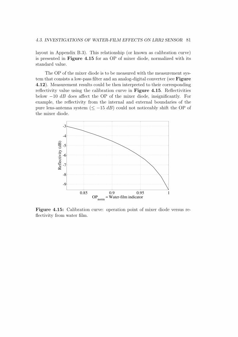
4.3. INVESTIGATIONS OF WATER-FILM EFFECTS ON LRR2 SENSOR 81
layout in Appendix B.3). This relationship (or known as calibration curve)is presented in Figure 4.15 for an OP of mixer diode, normalized with itsstandard value.
The OP of the mixer diode is to be measured with the measurement sys-tem that consists a low-pass filter and an analog-digital converter (see Figure4.12). Measurement results could be then interpreted to their correspondingreflectivity value using the calibration curve in Figure 4.15. Reflectivitiesbelow −10 dB does affect the OP of the mixer diode, insignificantly. Forexample, the reflectivity from the internal and external boundaries of thepure lens-antenna system (≤ −15 dB) could not noticeably shift the OP ofthe mixer diode.
0.85 0.9 0.95 1
-9
-8
-7
-6
-5
-4
-3
OPnorm ≈ Water-film indicator
Ref
lect
ivity
(dB
)
Figure 4.15: Calibration curve: operation point of mixer diode versus re-flectivity from water film.
82 4. EFFECTS OF WATER FILM ON MILLIMETER-WAVE RADAR
4.3.2 Results and discussions
Indication of the radar maximum detection range
A series of measurements have been performed using the system describedin section 4.3.1 and the calibration curve given in Figure 4.15. Some ofthe experimental data that has been taken to determine the reduction of themaximum detection range of the radar are shown in Figure 4.4 and Figure4.16.
In an air plan field with free of any other scatterers (except road-clutter),a triangular corner reflector with RCS = 3 m2 is placed as a radar target at adistance of more than 500 m from the test vehicle with the radar boresightedon the corner reflector. Note that a triangular corner reflector with improperangle alignment will degrade by 3 dB if all three edges deviate by 0.35λ or asingle edge deviates by 0.7λ [74]. The radar test vehicle is driven slowly withconstant speed towards this target along the radar boresighted and detectionparameters (like range, velocity and angle) of this target have been recorded.In the same way, a number of measurements have been performed with spraywater on the surface of the radome (Figure 4.10). The degree of wetnesson the radome surface is varied by regulating the flow rate of water througha water sprayer, which has been mounted at the top of the radome as wellas of the lens.
The target informations like velocity and angle are used only for control-ling the uniformity of the speed between measurements and the alignmentof target. The maximum detection range of the target for each measure-ment with spray water is normalized with the maximum detection range ofthe target with no water. These normalized detection range informationsare provided to Figure 4.4 with the corresponding reflectivities, which areextracted from the calibration curve in Figure 4.15. Note that, in themeasurement, the OP of the mixer diode is averaged over four mixer diodes(Figure 3.4) before normalization.
The presented measurement is relative in value and extreme care hasbeen taken to minimize an unavoidable sources of errors. The relative er-ror δ = 1%, given in the Figures 4.16 and 4.17, is consisted of externalinfluences like external temperature (causes signal-path expansion) and road-
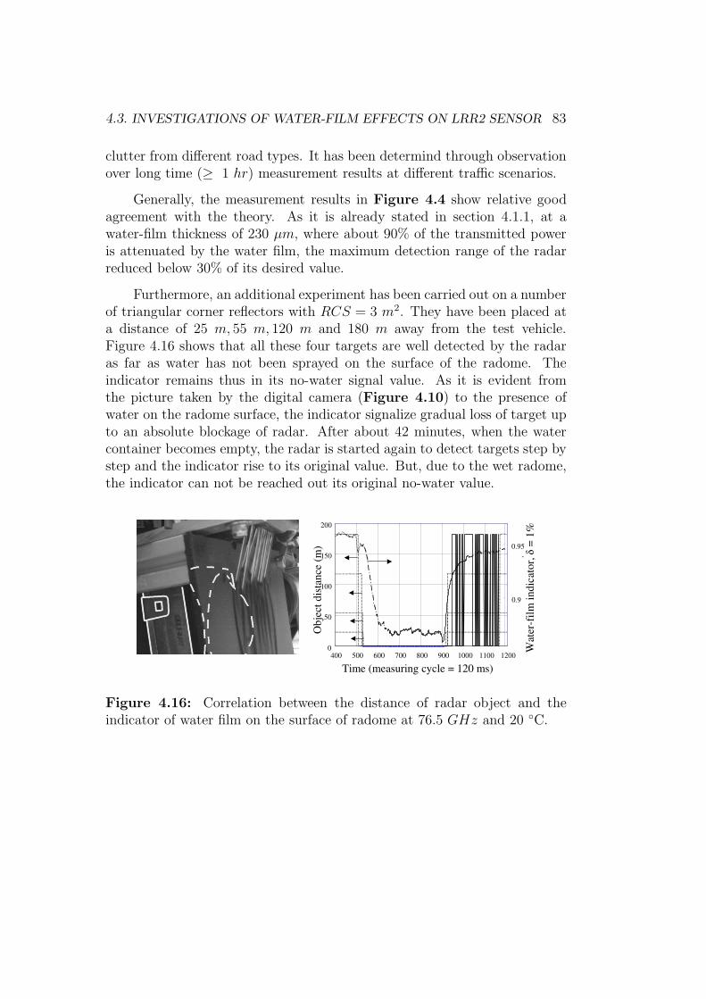
4.3. INVESTIGATIONS OF WATER-FILM EFFECTS ON LRR2 SENSOR 83
clutter from different road types. It has been determind through observationover long time (≥ 1 hr) measurement results at different traffic scenarios.
Generally, the measurement results in Figure 4.4 show relative goodagreement with the theory. As it is already stated in section 4.1.1, at awater-film thickness of 230 µm, where about 90% of the transmitted poweris attenuated by the water film, the maximum detection range of the radarreduced below 30% of its desired value.
Furthermore, an additional experiment has been carried out on a numberof triangular corner reflectors with RCS = 3 m2. They have been placed ata distance of 25 m, 55 m, 120 m and 180 m away from the test vehicle.Figure 4.16 shows that all these four targets are well detected by the radaras far as water has not been sprayed on the surface of the radome. Theindicator remains thus in its no-water signal value. As it is evident fromthe picture taken by the digital camera (Figure 4.10) to the presence ofwater on the radome surface, the indicator signalize gradual loss of target upto an absolute blockage of radar. After about 42 minutes, when the watercontainer becomes empty, the radar is started again to detect targets step bystep and the indicator rise to its original value. But, due to the wet radome,the indicator can not be reached out its original no-water value.
400 500 600 700 800 900 1000 1100 12000
50
100
150
200
Obj
ect d
ista
nce
(m)
0.9
0.95
Time (measuring cycle = 120 ms)
Wat
er-f
ilm in
dica
tor, δ=
1%
,
Figure 4.16: Correlation between the distance of radar object and theindicator of water film on the surface of radome at 76.5 GHz and 20 C.
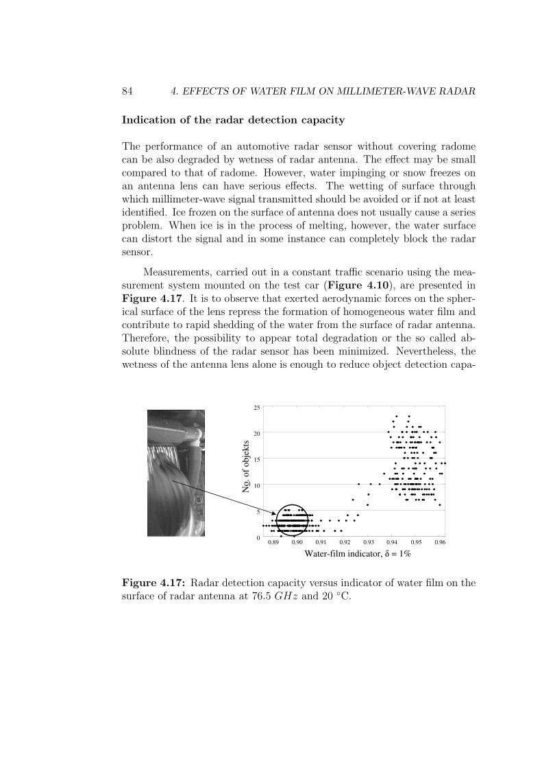
84 4. EFFECTS OF WATER FILM ON MILLIMETER-WAVE RADAR
Indication of the radar detection capacity
The performance of an automotive radar sensor without covering radomecan be also degraded by wetness of radar antenna. The effect may be smallcompared to that of radome. However, water impinging or snow freezes onan antenna lens can have serious effects. The wetting of surface throughwhich millimeter-wave signal transmitted should be avoided or if not at leastidentified. Ice frozen on the surface of antenna does not usually cause a seriesproblem. When ice is in the process of melting, however, the water surfacecan distort the signal and in some instance can completely block the radarsensor.
Measurements, carried out in a constant traffic scenario using the mea-surement system mounted on the test car (Figure 4.10), are presented inFigure 4.17. It is to observe that exerted aerodynamic forces on the spher-ical surface of the lens repress the formation of homogeneous water film andcontribute to rapid shedding of the water from the surface of radar antenna.Therefore, the possibility to appear total degradation or the so called ab-solute blindness of the radar sensor has been minimized. Nevertheless, thewetness of the antenna lens alone is enough to reduce object detection capa-
0.89 0.90 0.91 0.92 0.93 0.94 0.95 0.960
5
10
15
20
25
Water-film indicator, δ = 1%
No.
of o
bjek
ts
Figure 4.17: Radar detection capacity versus indicator of water film on thesurface of radar antenna at 76.5 GHz and 20 C.

4.3. INVESTIGATIONS OF WATER-FILM EFFECTS ON LRR2 SENSOR 85
bility of the radar to a certain extent. The number of detected objects bythe radar reduces significantly and becomes below 5 while water sprays onthe antenna lens. It has been greater than 10 as the radar antenna lens wasfree from water.
Chapter 5
Effects of rain onmillimeter-wave radar
The second major cause of millimeter-wave automotive radar signal degra-dation is that of the interaction of electromagnetic waves with rains in thepropagation medium. A lot of scientific work has been reported in the paston the significance of this interaction in the micro-wave and millimeter-waverange [10, 11, 13, 75, 76, 77, 78, 79, 80, 81]. These studies have been ob-tained quantitative data, which demonstrate that precipitation generally af-fects electromagnetic wave propagation at micro- and millimeter-wave fre-quencies and results in a considerable effect on the detection performance ofradars.
Some of the effects of precipitation on wave propagation have a directapplication to identify rain in the scanning view of a radar. Hence, the scopeof this chapter will be confined on hypothesis those enable the identificationof rain using automotive radar sensor by applying the theory given in § 2.3.This can be used as an indicator for the degree of possible degradation ofperformance and may be applied to deal with proper counteractions so thatavailability of automotive radar sensor could be assured at rainy weathercondition.
86
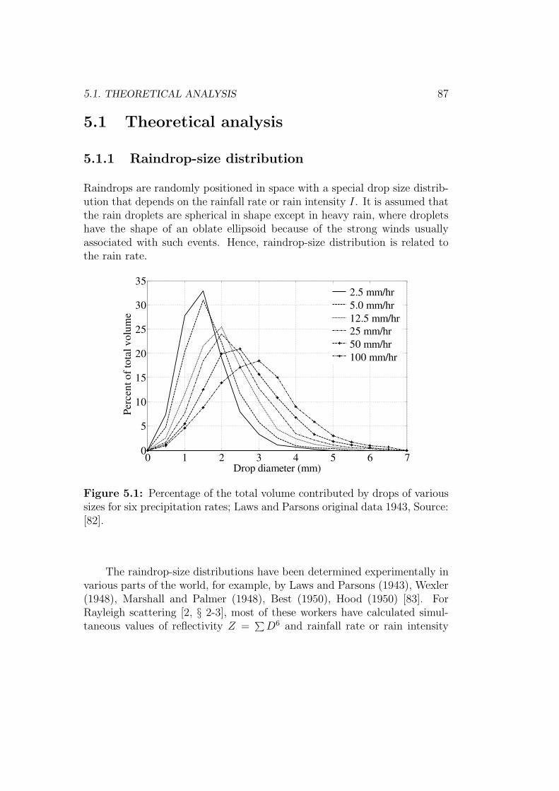
5.1. THEORETICAL ANALYSIS 87
5.1 Theoretical analysis
5.1.1 Raindrop-size distribution
Raindrops are randomly positioned in space with a special drop size distrib-ution that depends on the rainfall rate or rain intensity I. It is assumed thatthe rain droplets are spherical in shape except in heavy rain, where dropletshave the shape of an oblate ellipsoid because of the strong winds usuallyassociated with such events. Hence, raindrop-size distribution is related tothe rain rate.
0 1 2 3 4 5 6 70
5
10
15
20
25
30
35
Drop diameter (mm)
Perc
ent o
f tot
al v
olum
e
2.5 mm/hr 5.0 mm/hr 12.5 mm/hr 25 mm/hr 50 mm/hr 100 mm/hr
Figure 5.1: Percentage of the total volume contributed by drops of varioussizes for six precipitation rates; Laws and Parsons original data 1943, Source:[82].
The raindrop-size distributions have been determined experimentally invarious parts of the world, for example, by Laws and Parsons (1943), Wexler(1948), Marshall and Palmer (1948), Best (1950), Hood (1950) [83]. ForRayleigh scattering [2, § 2-3], most of these workers have calculated simul-taneous values of reflectivity Z =
∑
D6 and rainfall rate or rain intensity
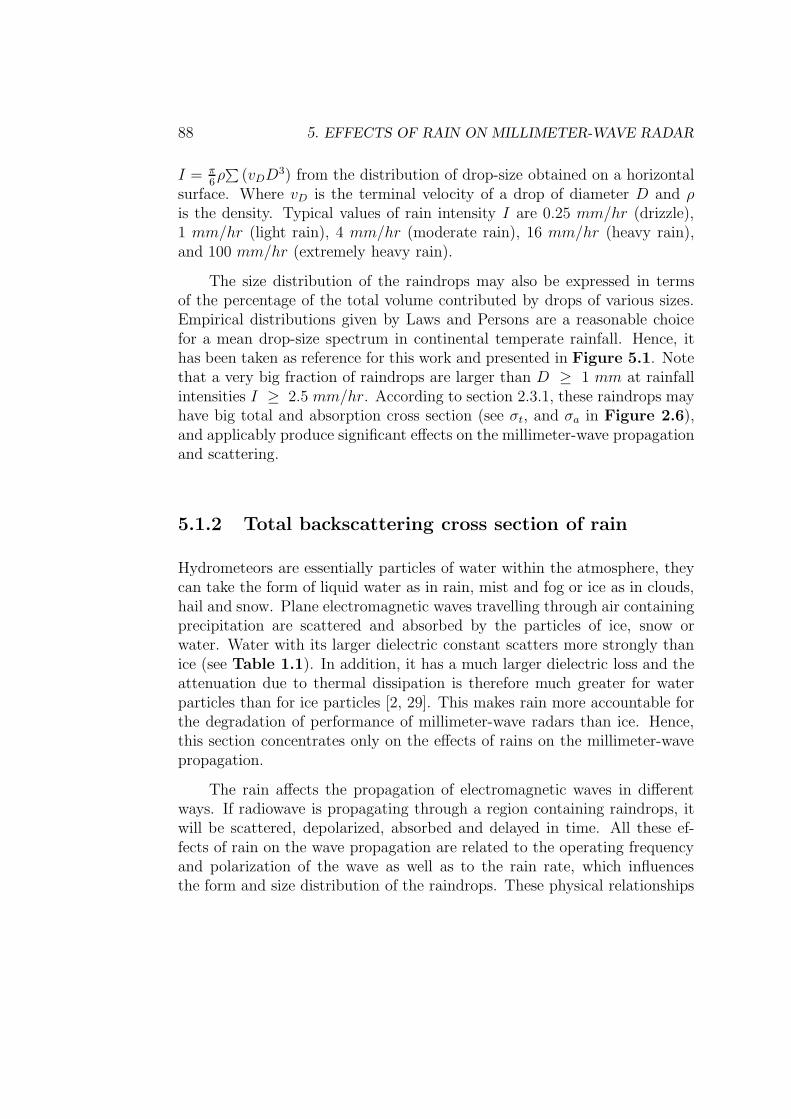
88 5. EFFECTS OF RAIN ON MILLIMETER-WAVE RADAR
I = π6ρ∑
(vDD3) from the distribution of drop-size obtained on a horizontal
surface. Where vD is the terminal velocity of a drop of diameter D and ρis the density. Typical values of rain intensity I are 0.25 mm/hr (drizzle),1 mm/hr (light rain), 4 mm/hr (moderate rain), 16 mm/hr (heavy rain),and 100 mm/hr (extremely heavy rain).
The size distribution of the raindrops may also be expressed in termsof the percentage of the total volume contributed by drops of various sizes.Empirical distributions given by Laws and Persons are a reasonable choicefor a mean drop-size spectrum in continental temperate rainfall. Hence, ithas been taken as reference for this work and presented in Figure 5.1. Notethat a very big fraction of raindrops are larger than D ≥ 1 mm at rainfallintensities I ≥ 2.5 mm/hr. According to section 2.3.1, these raindrops mayhave big total and absorption cross section (see σt, and σa in Figure 2.6),and applicably produce significant effects on the millimeter-wave propagationand scattering.
5.1.2 Total backscattering cross section of rain
Hydrometeors are essentially particles of water within the atmosphere, theycan take the form of liquid water as in rain, mist and fog or ice as in clouds,hail and snow. Plane electromagnetic waves travelling through air containingprecipitation are scattered and absorbed by the particles of ice, snow orwater. Water with its larger dielectric constant scatters more strongly thanice (see Table 1.1). In addition, it has a much larger dielectric loss and theattenuation due to thermal dissipation is therefore much greater for waterparticles than for ice particles [2, 29]. This makes rain more accountable forthe degradation of performance of millimeter-wave radars than ice. Hence,this section concentrates only on the effects of rains on the millimeter-wavepropagation.
The rain affects the propagation of electromagnetic waves in differentways. If radiowave is propagating through a region containing raindrops, itwill be scattered, depolarized, absorbed and delayed in time. All these ef-fects of rain on the wave propagation are related to the operating frequencyand polarization of the wave as well as to the rain rate, which influencesthe form and size distribution of the raindrops. These physical relationships
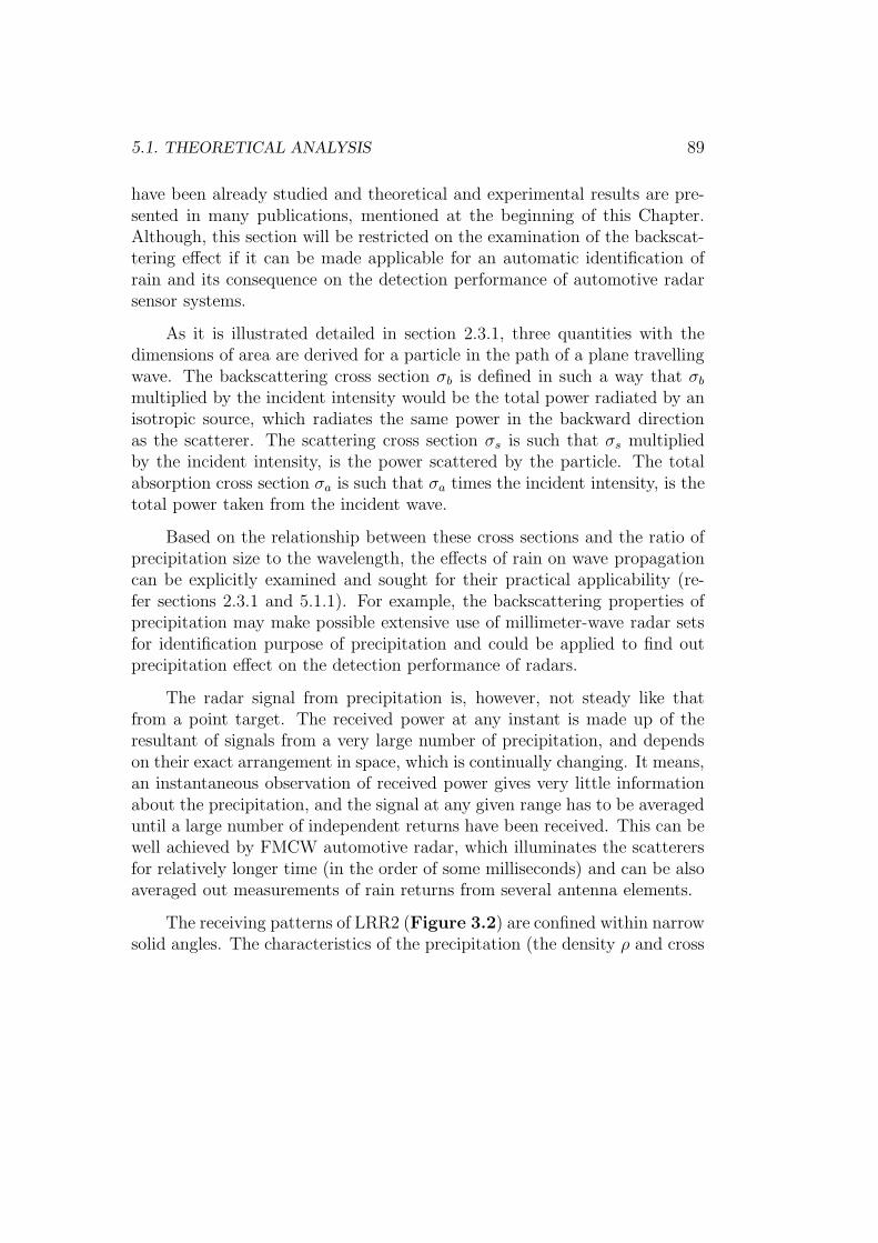
5.1. THEORETICAL ANALYSIS 89
have been already studied and theoretical and experimental results are pre-sented in many publications, mentioned at the beginning of this Chapter.Although, this section will be restricted on the examination of the backscat-tering effect if it can be made applicable for an automatic identification ofrain and its consequence on the detection performance of automotive radarsensor systems.
As it is illustrated detailed in section 2.3.1, three quantities with thedimensions of area are derived for a particle in the path of a plane travellingwave. The backscattering cross section σb is defined in such a way that σb
multiplied by the incident intensity would be the total power radiated by anisotropic source, which radiates the same power in the backward directionas the scatterer. The scattering cross section σs is such that σs multipliedby the incident intensity, is the power scattered by the particle. The totalabsorption cross section σa is such that σa times the incident intensity, is thetotal power taken from the incident wave.
Based on the relationship between these cross sections and the ratio ofprecipitation size to the wavelength, the effects of rain on wave propagationcan be explicitly examined and sought for their practical applicability (re-fer sections 2.3.1 and 5.1.1). For example, the backscattering properties ofprecipitation may make possible extensive use of millimeter-wave radar setsfor identification purpose of precipitation and could be applied to find outprecipitation effect on the detection performance of radars.
The radar signal from precipitation is, however, not steady like thatfrom a point target. The received power at any instant is made up of theresultant of signals from a very large number of precipitation, and dependson their exact arrangement in space, which is continually changing. It means,an instantaneous observation of received power gives very little informationabout the precipitation, and the signal at any given range has to be averageduntil a large number of independent returns have been received. This can bewell achieved by FMCW automotive radar, which illuminates the scatterersfor relatively longer time (in the order of some milliseconds) and can be alsoaveraged out measurements of rain returns from several antenna elements.
The receiving patterns of LRR2 (Figure 3.2) are confined within narrowsolid angles. The characteristics of the precipitation (the density ρ and cross
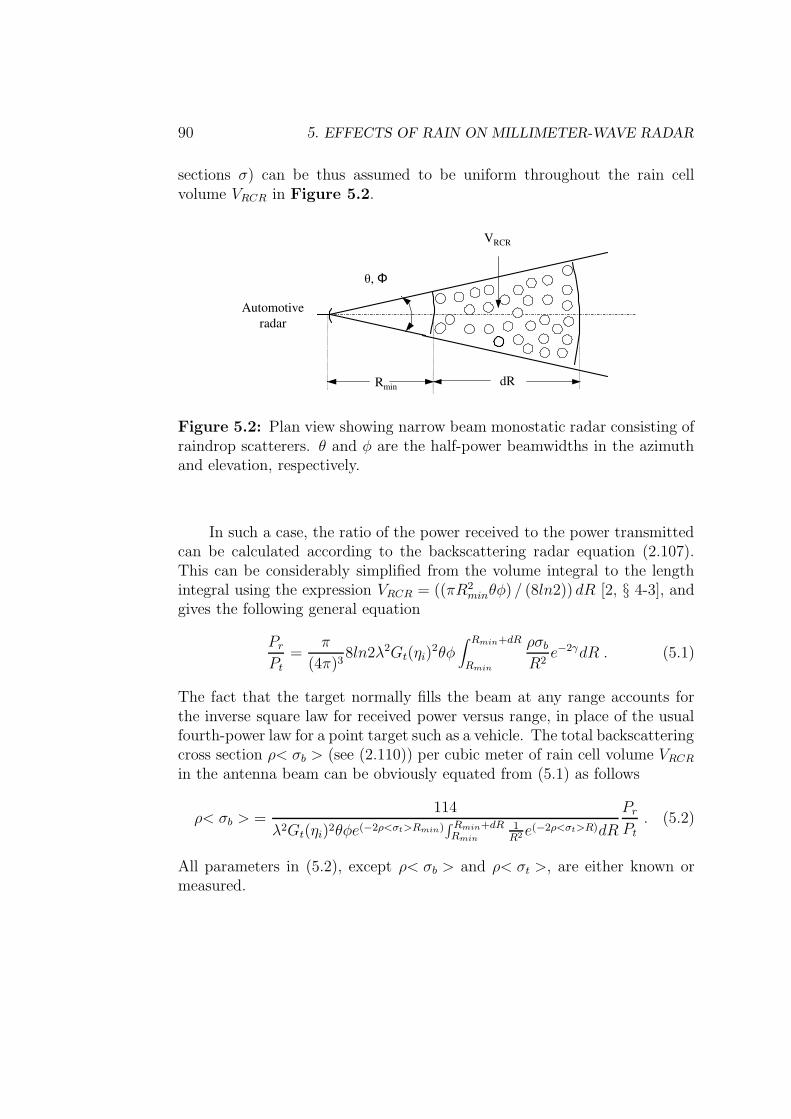
90 5. EFFECTS OF RAIN ON MILLIMETER-WAVE RADAR
sections σ) can be thus assumed to be uniform throughout the rain cellvolume VRCR in Figure 5.2.
Automotive radar
dRRmin
VRCR
θ, Φ
Figure 5.2: Plan view showing narrow beam monostatic radar consisting ofraindrop scatterers. θ and φ are the half-power beamwidths in the azimuthand elevation, respectively.
In such a case, the ratio of the power received to the power transmittedcan be calculated according to the backscattering radar equation (2.107).This can be considerably simplified from the volume integral to the lengthintegral using the expression VRCR = ((πR2
minθφ) / (8ln2)) dR [2, § 4-3], andgives the following general equation
Pr
Pt
=π
(4π)38ln2λ2Gt(ηi)
2θφ∫ Rmin+dR
Rmin
ρσb
R2e−2γdR . (5.1)
The fact that the target normally fills the beam at any range accounts forthe inverse square law for received power versus range, in place of the usualfourth-power law for a point target such as a vehicle. The total backscatteringcross section ρ< σb > (see (2.110)) per cubic meter of rain cell volume VRCR
in the antenna beam can be obviously equated from (5.1) as follows
ρ< σb > =114
λ2Gt(ηi)2θφe(−2ρ<σt>Rmin)∫ Rmin+dRRmin
1R2 e(−2ρ<σt>R)dR
Pr
Pt
. (5.2)
All parameters in (5.2), except ρ< σb > and ρ< σt >, are either known ormeasured.
5.2. EXPERIMENTAL INVESTIGATIONS OF RAIN EFFECTS 91
In case of millimeter-wave radar, Mie scattering occurs since most ofthe raindrops are in the order of the size of the wavelength (Figure 5.1).And then, the calculations of the cross sections can be treated by the Mie-theory [2, § 2-8]. The optical distance γ in (5.1) can also expressed with theattenuation due to rain ρ< σt > (see (2.108)). This is nearly proportionalto the rain intensity I and given by ρ< σt > = KtI. The constant Kt, onthe other hand, depends on the rain intensity I and some typical valuesare given in [2, § 3-2]. For millimeter and optical frequencies, Kt ≈ 0.4 −0.8 dB/km/mm/hr at rainfall intensities I < 10 mm/hr, and Kt decreasesto 0.15 − 0.3 dB/km/mm/hr at rainfall intensities I > 10 mm/hr.
So far, the attenuating effect of the precipitation e−2γ , through whichthe signal may have to pass, has been considered. It shows that the influenceof the rain intensity over the attenuation makes it difficult to determine thebackscattering cross section ρ< σb > of the rain using (5.2) by only measuringthe received power.
For precipitation that is found in near distance to the radar sensor, itcould be, however, possible to neglect the attenuation term in (5.2). Thatis, ρ< σb > can be approximated as a function of rain intensity I by measur-ing the average backscattered power Pr. Experimental investigation on thisrelationship will be presented and discussed in detail in the next section.
5.2 Experimental investigations of rain effects
Since the effects of rain on the wave propagation are generally correlated toeach other over the rainfall intensity, the ability to measure returned signalfrom rain may lead to find out the loss of the signal-to-noise ratio of a radartarget. Note that the signal-to-noise ratio is one of the main parameter interms of which the detection performance of a radar sensor could be judged[39].
The receiver sensitivity of an automotive radar is enough to detect asmall amount of power returned from scatterers like raindrops. Obviously,the less the distance of the scatterers from the radar, the more a radar isable to detect smaller or less efficient scatterers due to less antenna beamspreading loss.
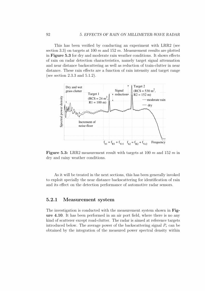
92 5. EFFECTS OF RAIN ON MILLIMETER-WAVE RADAR
This has been verified by conducting an experiment with LRR2 (seesection 3.3) on targets at 100 m and 152 m. Measurement results are plottedin Figure 5.3 for dry and moderate rain weather conditions. It shows effectsof rain on radar detection characteristics, namely target signal attenuationand near distance backscattering as well as reduction of train-clutter in neardistance. These rain effects are a function of rain intensity and target range(see section 2.3.3 and 5.1.2).
Frequency
Spec
tral
pow
er d
ensi
ty
Target 2 (RCS = 530 m2, R2 = 152 m) Target 1
(RCS = 24 m2, R1 = 100 m)
moderate rain
dry
Signalreduction
Increment ofnoise-floor
fb1 = fR1 + fVr1 fb2 = fR2 + fVr2
Dry and wetgrass clutter
Figure 5.3: LRR2 measurement result with targets at 100 m and 152 m indry and rainy weather conditions.
As it will be treated in the next sections, this has been generally invokedto exploit specially the near distance backscattering for identification of rainand its effect on the detection performance of automotive radar sensors.
5.2.1 Measurement system
The investigation is conducted with the measurement system shown in Fig-ure 4.10. It has been performed in an air port field, where there is no anykind of scatterer except road-clutter. The radar is aimed at reference targetsintroduced below. The average power of the backscattering signal Pr can beobtained by the integration of the measured power spectral density within
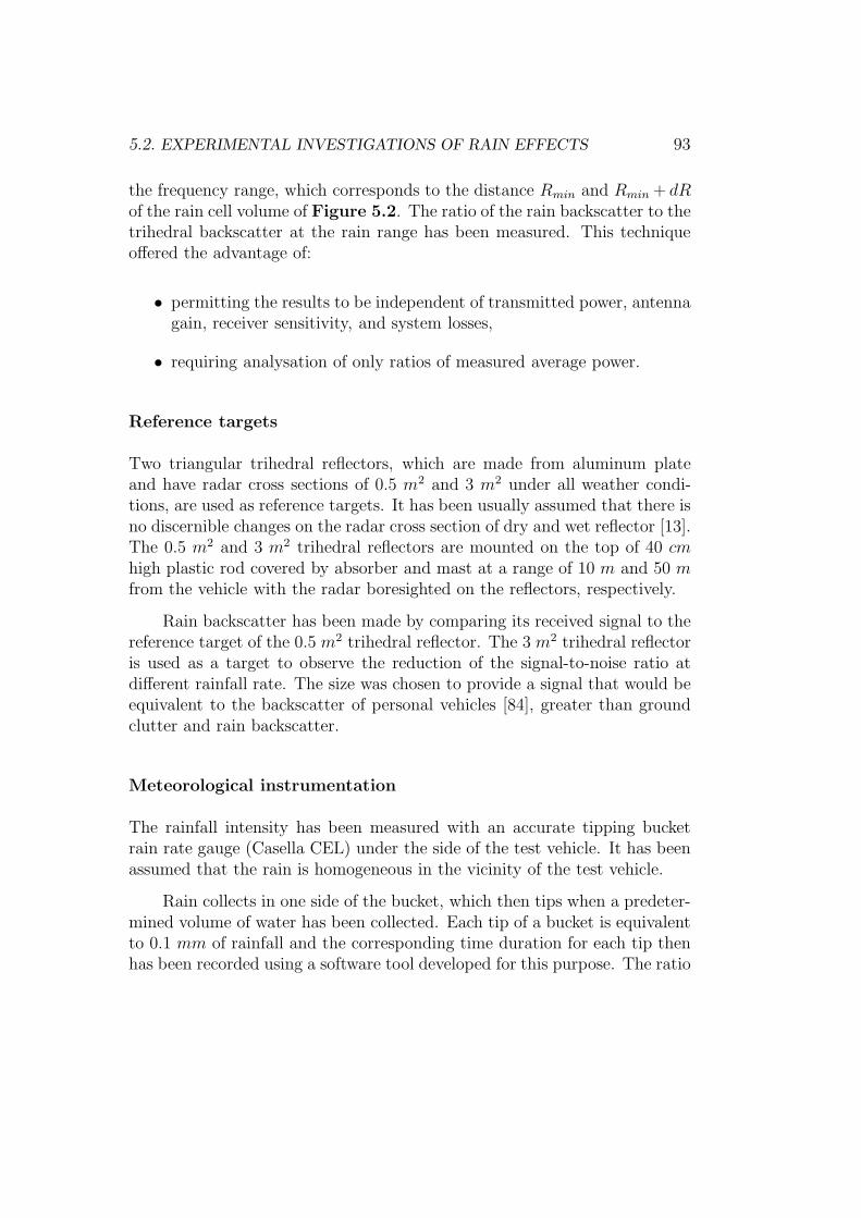
5.2. EXPERIMENTAL INVESTIGATIONS OF RAIN EFFECTS 93
the frequency range, which corresponds to the distance Rmin and Rmin + dRof the rain cell volume of Figure 5.2. The ratio of the rain backscatter to thetrihedral backscatter at the rain range has been measured. This techniqueoffered the advantage of:
• permitting the results to be independent of transmitted power, antennagain, receiver sensitivity, and system losses,
• requiring analysation of only ratios of measured average power.
Reference targets
Two triangular trihedral reflectors, which are made from aluminum plateand have radar cross sections of 0.5 m2 and 3 m2 under all weather condi-tions, are used as reference targets. It has been usually assumed that there isno discernible changes on the radar cross section of dry and wet reflector [13].The 0.5 m2 and 3 m2 trihedral reflectors are mounted on the top of 40 cmhigh plastic rod covered by absorber and mast at a range of 10 m and 50 mfrom the vehicle with the radar boresighted on the reflectors, respectively.
Rain backscatter has been made by comparing its received signal to thereference target of the 0.5 m2 trihedral reflector. The 3 m2 trihedral reflectoris used as a target to observe the reduction of the signal-to-noise ratio atdifferent rainfall rate. The size was chosen to provide a signal that would beequivalent to the backscatter of personal vehicles [84], greater than groundclutter and rain backscatter.
Meteorological instrumentation
The rainfall intensity has been measured with an accurate tipping bucketrain rate gauge (Casella CEL) under the side of the test vehicle. It has beenassumed that the rain is homogeneous in the vicinity of the test vehicle.
Rain collects in one side of the bucket, which then tips when a predeter-mined volume of water has been collected. Each tip of a bucket is equivalentto 0.1 mm of rainfall and the corresponding time duration for each tip thenhas been recorded using a software tool developed for this purpose. The ratio
94 5. EFFECTS OF RAIN ON MILLIMETER-WAVE RADAR
of the depth (0.1 mm) to the recorded accumulation time (in hours) givesthen the intensity of rain in mm/hr. Figure 5.4 presents the rainfall ratemeasured with this rain gauge at an air port field station.
0.00
20.00
40.00
60.00
80.00
100.00
120.00
140.00
160.00
19:
23:0
6
19:
23:2
7
19:
23:4
8
19:
24:0
9
19:
24:3
2
19:
25:3
8
19:
26:5
8
19:
28:5
0
19:
30:2
4
19:
32:3
3
19:
36:1
8
19:
39:3
9
19:
42:5
1
19:
46:0
7
19:
49:3
2
19:
52:0
7
19:
53:4
4
Time (hr: min: sec)
Rai
nfal
l rat
e (m
m/h
r)
Figure 5.4: Rainfall rate measured on the 29th of July 2005 at theMalmsheim air port, Baden-Wurttemberg, Germany.
These data points represent measurements made during rainstorm oc-curring once on the 29th of July 2005 between 19 : 20 and 20 : 00 hr. Thus, avariety of meteorological conditions are not involved. The rainstorm is gen-erally of short, heavy shower type where there was an intense onset of rainfollowed by a slow tapering off. The temperature during the measurementwas about 28 C. Because of the relatively short time required to accumu-late enough rain to tip the bucket (i.e. 7.2 sec for 50 mm/hr and 3.6 sec for100 mm/hr), the data from a tipping bucket gauge were most accurate forrainfall rate below 50 mm/hr.
5.2. EXPERIMENTAL INVESTIGATIONS OF RAIN EFFECTS 95
5.2.2 Results and discussions
Average rain backscattering cross section
As previously pointed out, the average rain backscattering cross sectionρ< σb > per unit volume has been computed from the ratio of measuredaverage power of the rain backscatter to the reference target at the middleof the rain cell volume as follows
ρ< σb > =σRT
VRCR
PrR
PrRT
, (5.3)
where σRT is the radar cross section of the reference target (0.5 m2), VRCR isthe rain cell volume, and PrR, PrRT are measured average backscatter powerof the rain and the reference target, respectively. For both measurements,the same transmitted power Pt has been assumed. The rain cell volumehas been chosen in a short distance between the range Rmin = 5 m andRmin + dR = 15 m (Figure 5.2) so that rain attenuation could be keptminimum and negligible. In addition to that, performing a short distancemeasurement of rain backscattering is in favour of receiving larger rain returnbecause of less antenna beam spreading loss.
Variability of the rain backscatter for a given rainfall intensity is ex-pected because radar echo power from precipitation is a function of manyvariable parameters like number, size distribution, shape, and location ofraindrops within the rain cell volume at any given moment. In order to geta more steady representative value, it was meaningful to average returnedpower from a number of consecutive measurements for each rainfall intensity.This is additional to what the radar weights with relative longtime (> 1 ms)illumination of scatterers.
Measured average rain backscattering cross section data are presentedin Figure 5.5 in a logarithm scale. A least squares power fit of a first-orderpolynomial is made to these data ρ< σb >. The equation for this curves isof the form Z = aIb, where Z is referred to as radar reflectivity in m2/m3.The regression coefficients, a and b have been found 0.00224 and 0.99454 asthe best fit values for this rain type and location.
During the measurement, the rain has brought a storming windy air,which caused a strong fluctuation of rainfall intensities, particularly for mea-surements above 50 mm/hr (Figure 5.4). Therefore, it was difficult to
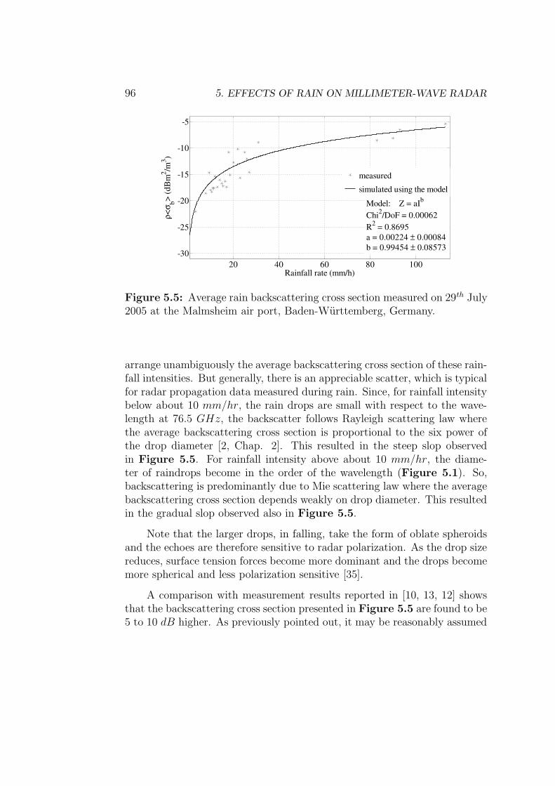
96 5. EFFECTS OF RAIN ON MILLIMETER-WAVE RADAR
20 40 60 80 100-30
-25
-20
-15
-10
-5
Rainfall rate (mm/h)
ρ <σ b>
(dB
m2 /m
3 ) measured
simulated using the model
Model: Z = aIb
Chi2/DoF = 0.00062R2 = 0.8695a = 0.00224 ± 0.00084b = 0.99454 ± 0.08573
Figure 5.5: Average rain backscattering cross section measured on 29th July2005 at the Malmsheim air port, Baden-Wurttemberg, Germany.
arrange unambiguously the average backscattering cross section of these rain-fall intensities. But generally, there is an appreciable scatter, which is typicalfor radar propagation data measured during rain. Since, for rainfall intensitybelow about 10 mm/hr, the rain drops are small with respect to the wave-length at 76.5 GHz, the backscatter follows Rayleigh scattering law wherethe average backscattering cross section is proportional to the six power ofthe drop diameter [2, Chap. 2]. This resulted in the steep slop observedin Figure 5.5. For rainfall intensity above about 10 mm/hr, the diame-ter of raindrops become in the order of the wavelength (Figure 5.1). So,backscattering is predominantly due to Mie scattering law where the averagebackscattering cross section depends weakly on drop diameter. This resultedin the gradual slop observed also in Figure 5.5.
Note that the larger drops, in falling, take the form of oblate spheroidsand the echoes are therefore sensitive to radar polarization. As the drop sizereduces, surface tension forces become more dominant and the drops becomemore spherical and less polarization sensitive [35].
A comparison with measurement results reported in [10, 13, 12] showsthat the backscattering cross section presented in Figure 5.5 are found to be5 to 10 dB higher. As previously pointed out, it may be reasonably assumed
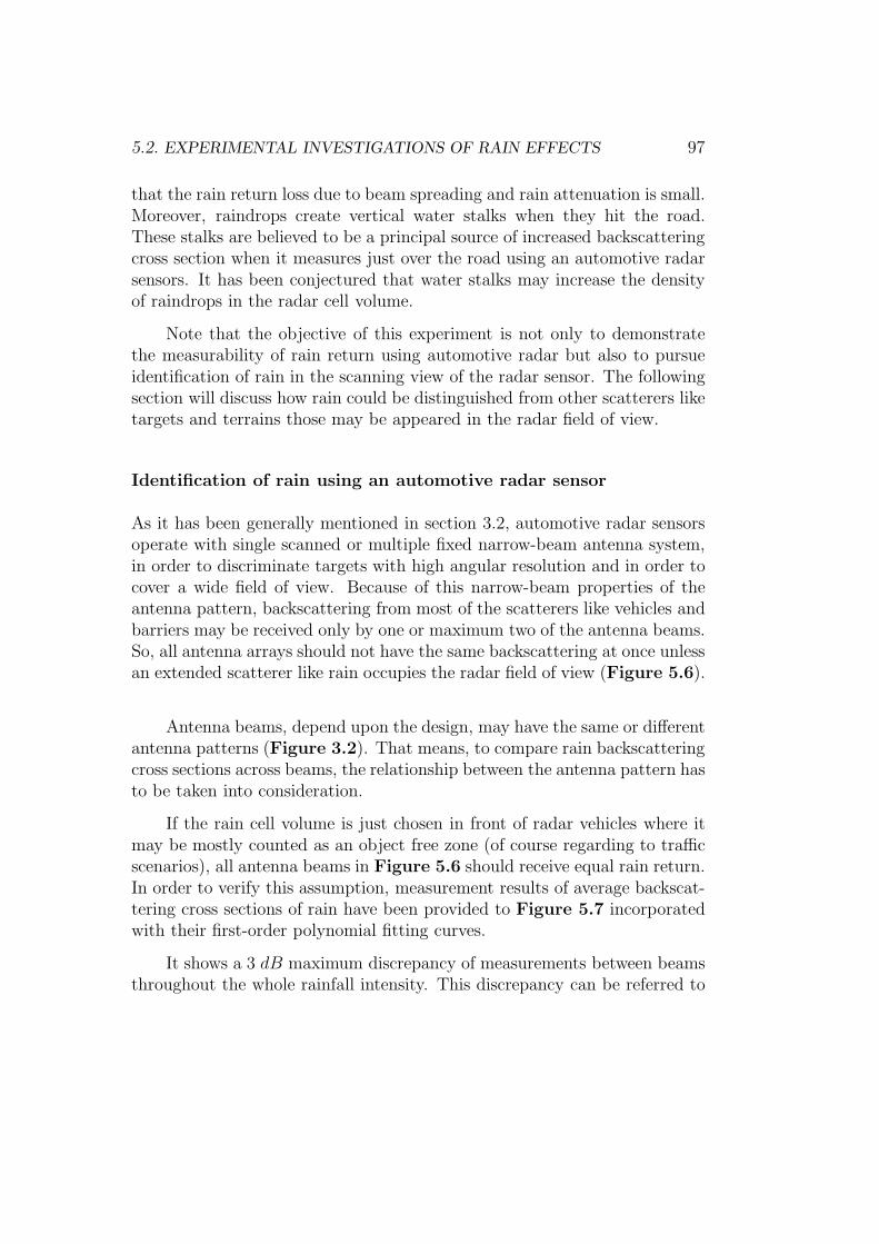
5.2. EXPERIMENTAL INVESTIGATIONS OF RAIN EFFECTS 97
that the rain return loss due to beam spreading and rain attenuation is small.Moreover, raindrops create vertical water stalks when they hit the road.These stalks are believed to be a principal source of increased backscatteringcross section when it measures just over the road using an automotive radarsensors. It has been conjectured that water stalks may increase the densityof raindrops in the radar cell volume.
Note that the objective of this experiment is not only to demonstratethe measurability of rain return using automotive radar but also to pursueidentification of rain in the scanning view of the radar sensor. The followingsection will discuss how rain could be distinguished from other scatterers liketargets and terrains those may be appeared in the radar field of view.
Identification of rain using an automotive radar sensor
As it has been generally mentioned in section 3.2, automotive radar sensorsoperate with single scanned or multiple fixed narrow-beam antenna system,in order to discriminate targets with high angular resolution and in order tocover a wide field of view. Because of this narrow-beam properties of theantenna pattern, backscattering from most of the scatterers like vehicles andbarriers may be received only by one or maximum two of the antenna beams.So, all antenna arrays should not have the same backscattering at once unlessan extended scatterer like rain occupies the radar field of view (Figure 5.6).
Antenna beams, depend upon the design, may have the same or differentantenna patterns (Figure 3.2). That means, to compare rain backscatteringcross sections across beams, the relationship between the antenna pattern hasto be taken into consideration.
If the rain cell volume is just chosen in front of radar vehicles where itmay be mostly counted as an object free zone (of course regarding to trafficscenarios), all antenna beams in Figure 5.6 should receive equal rain return.In order to verify this assumption, measurement results of average backscat-tering cross sections of rain have been provided to Figure 5.7 incorporatedwith their first-order polynomial fitting curves.
It shows a 3 dB maximum discrepancy of measurements between beamsthroughout the whole rainfall intensity. This discrepancy can be referred to
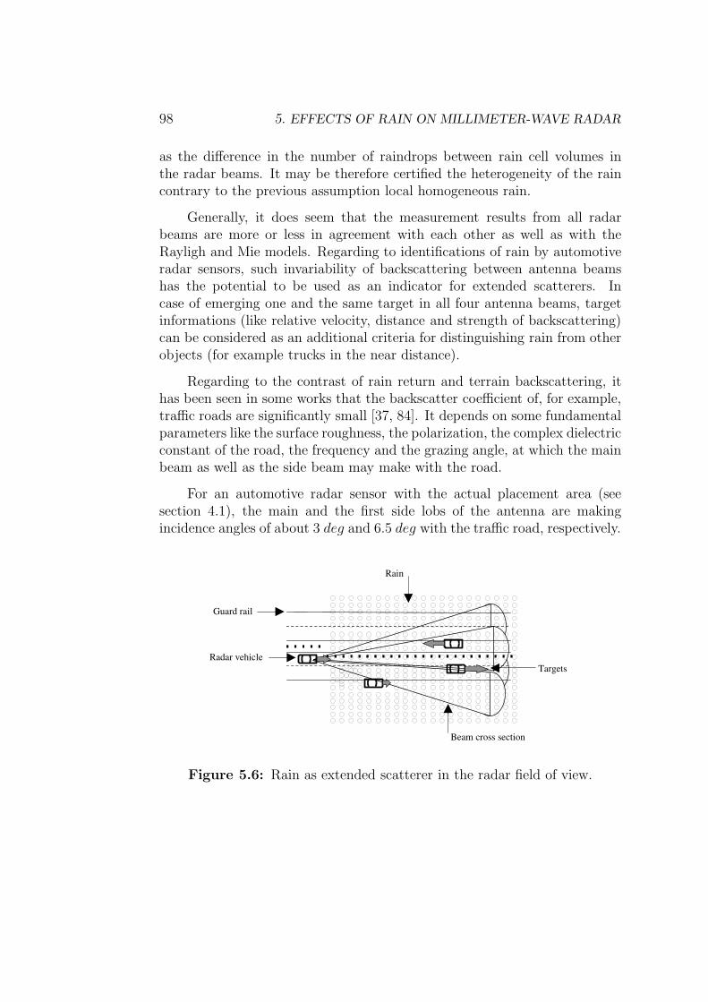
98 5. EFFECTS OF RAIN ON MILLIMETER-WAVE RADAR
as the difference in the number of raindrops between rain cell volumes inthe radar beams. It may be therefore certified the heterogeneity of the raincontrary to the previous assumption local homogeneous rain.
Generally, it does seem that the measurement results from all radarbeams are more or less in agreement with each other as well as with theRayligh and Mie models. Regarding to identifications of rain by automotiveradar sensors, such invariability of backscattering between antenna beamshas the potential to be used as an indicator for extended scatterers. Incase of emerging one and the same target in all four antenna beams, targetinformations (like relative velocity, distance and strength of backscattering)can be considered as an additional criteria for distinguishing rain from otherobjects (for example trucks in the near distance).
Regarding to the contrast of rain return and terrain backscattering, ithas been seen in some works that the backscatter coefficient of, for example,traffic roads are significantly small [37, 84]. It depends on some fundamentalparameters like the surface roughness, the polarization, the complex dielectricconstant of the road, the frequency and the grazing angle, at which the mainbeam as well as the side beam may make with the road.
For an automotive radar sensor with the actual placement area (seesection 4.1), the main and the first side lobs of the antenna are makingincidence angles of about 3 deg and 6.5 deg with the traffic road, respectively.
Radar vehicleTargets
Beam cross section
Rain
Guard rail
Figure 5.6: Rain as extended scatterer in the radar field of view.
5.2. EXPERIMENTAL INVESTIGATIONS OF RAIN EFFECTS 99
20 40 60 80 100-30
-25
-20
-15
-10
-5
Rainfall intensity (mm/hr)
ρ <σ b>
(dB
m2 /m
3 ) beam 1 measured
beam 2 measured
beam 3 measured
beam 4 measured
beam 1 simulated
beam 2 simulated
beam 3 simulated
beam 4 simulated
Model: Z = aIb
beam 1: Chi2/DoF = 0.00058, R2 = 0.83147, a = 0.00565 ± 0.00165, b = 0.76457 ± 0.07015beam 2: Chi2/DoF = 0.00047, R2 = 0.87114, a = 0.00245 ± 0.00085, b = 0.94823 ± 0.07931beam 3: Chi2/DoF = 0.00073, R2 = 0.85296, a = 0.00154 ± 0.00071, b = 1.07694 ± 0.10406beam 4: Chi2/DoF = 0.00057, R2 = 0.91571, a = 0.00102 ± 0.0042, b = 1.20238 ± 0.09168
Figure 5.7: Four beam average rain backscattering cross section measuredon 29th July 2005 at the Malmsheim air port, Baden-Wurttemberg, Germany.
This may produce a maximum backscattering cross section, for example, ofasphalt road lower than −40 dBm2 [46, § 4.1]. That means, for rainfallintensities higher than 4 mm/hr, the backscattering cross section of rain andtherefore its identification may not be disfigured with road returns (Figure5.7). Note that, as it will be discussed in the section below, these rainfallintensities are only accountable for significant loss of the signal-to-noise ratio.
Loss of the signal-to-noise ratio due to rain
The effects of rain on the detection performance of a radar may be gener-ally observed through probe the reduction of the signal-to-noise ratio. As ithas been demonstrated in Figure 5.3, this is the result of signal attenuationand increment of noise floor due to rain returns throughout the measurementrange of the radar.
Note that signal attenuation due to rain is a mixture of scatter loss andabsorption. Note also that the scattering and absorption cross sections area function of the relationship between the raindrop-size and the wavelength(Figure 2.6). Hence, the signal-to-noise ratio has been investigated as afunction of the rainfall intensity.
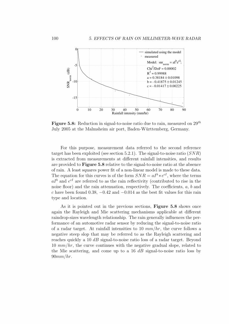
100 5. EFFECTS OF RAIN ON MILLIMETER-WAVE RADAR
0 10 20 30 40 50 60 70 80 90
-15
-10
-5
0
Rainfall intensity (mm/hr)
SNR
norm
(dB
)
simulated using the model measured
Model: snrnorm = aIbecI;
Chi2/DoF = 0.00002R2 = 0.99988a = 0.38184 ± 0.01098b = - 0.41875 ± 0.01245c = - 0.01417 ± 0.00225
Figure 5.8: Reduction in signal-to-noise ratio due to rain, measured on 29th
July 2005 at the Malmsheim air port, Baden-Wurttemberg, Germany.
For this purpose, measurement data referred to the second referencetarget has been exploited (see section 5.2.1). The signal-to-noise ratio (SNR)is extracted from measurements at different rainfall intensities, and resultsare provided to Figure 5.8 relative to the signal-to-noise ratio at the absenceof rain. A least squares power fit of a non-linear model is made to these data.The equation for this curves is of the form SNR = aI b ∗ ecI , where the termsaIb and ecI are referred to as the rain reflectivity (contributed to rise in thenoise floor) and the rain attenuation, respectively. The coefficients, a, b andc have been found 0.38, −0.42 and −0.014 as the best fit values for this raintype and location.
As it is pointed out in the previous sections, Figure 5.8 shows onceagain the Rayleigh and Mie scattering mechanisms applicable at differentraindrop-sizes wavelength relationship. The rain generally influences the per-formance of an automotive radar sensor by reducing the signal-to-noise ratioof a radar target. At rainfall intensities to 10 mm/hr, the curve follows anegative steep slop that may be referred to as the Rayleigh scattering andreaches quickly a 10 dB signal-to-noise ratio loss of a radar target. Beyond10 mm/hr, the curve continues with the negative gradual slope, related tothe Mie scattering, and come up to a 16 dB signal-to-noise ratio loss by90mm/hr.
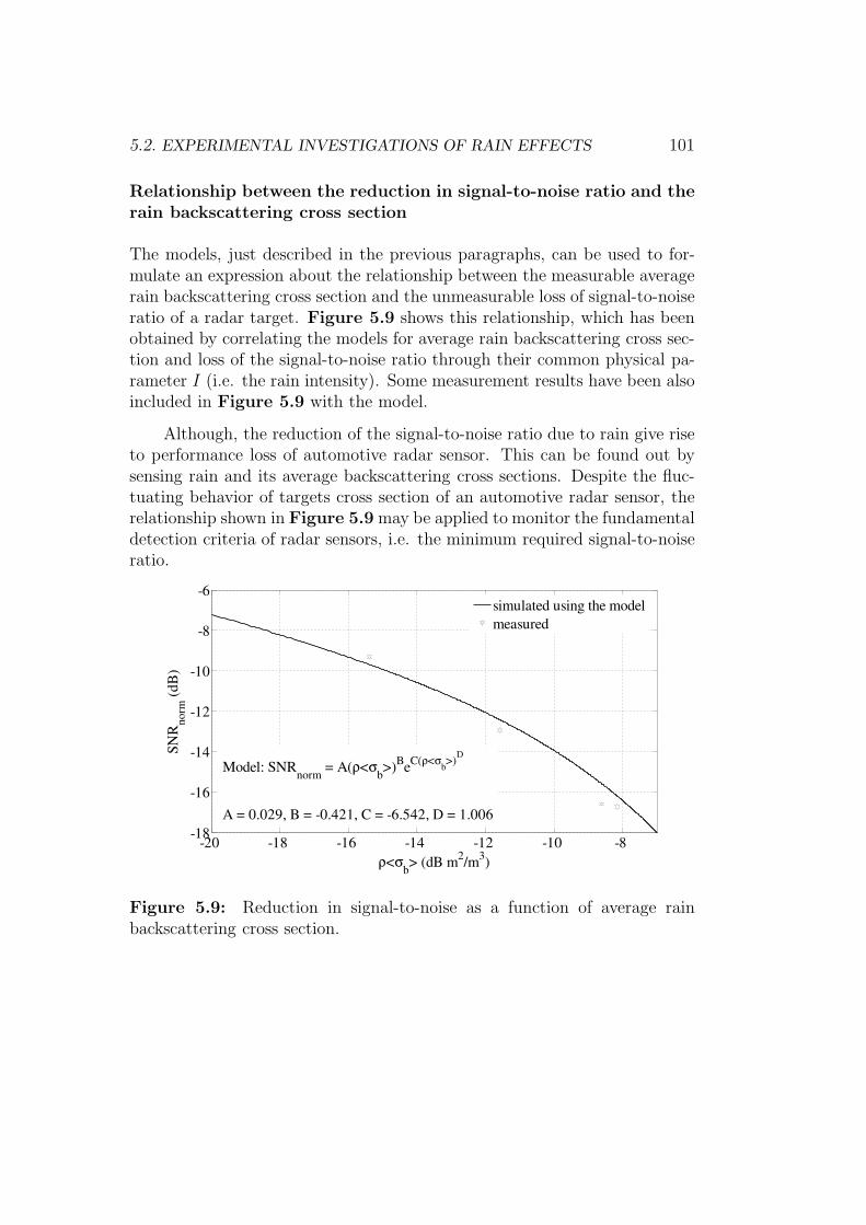
5.2. EXPERIMENTAL INVESTIGATIONS OF RAIN EFFECTS 101
Relationship between the reduction in signal-to-noise ratio and therain backscattering cross section
The models, just described in the previous paragraphs, can be used to for-mulate an expression about the relationship between the measurable averagerain backscattering cross section and the unmeasurable loss of signal-to-noiseratio of a radar target. Figure 5.9 shows this relationship, which has beenobtained by correlating the models for average rain backscattering cross sec-tion and loss of the signal-to-noise ratio through their common physical pa-rameter I (i.e. the rain intensity). Some measurement results have been alsoincluded in Figure 5.9 with the model.
Although, the reduction of the signal-to-noise ratio due to rain give riseto performance loss of automotive radar sensor. This can be found out bysensing rain and its average backscattering cross sections. Despite the fluc-tuating behavior of targets cross section of an automotive radar sensor, therelationship shown in Figure 5.9 may be applied to monitor the fundamentaldetection criteria of radar sensors, i.e. the minimum required signal-to-noiseratio.
-20 -18 -16 -14 -12 -10 -8-18
-16
-14
-12
-10
-8
-6
ρ<σb> (dB m2/m3)
SNR
norm
(dB
)
simulated using the modelmeasured
Model: SNRnorm = A(ρ<σb>)BeC(ρ<σ
b>)D
A = 0.029, B = -0.421, C = -6.542, D = 1.006
Figure 5.9: Reduction in signal-to-noise as a function of average rainbackscattering cross section.
Chapter 6
Conclusions
The most immediate, and perhaps the most important use that can be ap-plied from results of this work is in the design of millimeter-wave automotiveradar sensors, which have also to operate in adverse weather conditions.
It has been pointed out that the employment of automotive radar sensorsfor safety-oriented applications (collision mitigation, warning and avoidancesystems) requires a reliable performance at all weather conditions. Here twoof the key factors that must be taken into consideration in adverse weatherconditions, and their immediate recognition by millimeter wave based radar,will be briefly reviewed. The possible counteractions against the effect ofthese factors on operation of automotive radar sensors will be also remarked.
Two of the prime considerations in adverse weather conditions are thewater film on the surface of antenna or its covering and rain in the propaga-tion path of radar signals. Theoretical and experimental results of this workhave been intelligibly expressed that the presence of these two factors mayconsiderably affect detection characteristics of automotive radar sensors. Ithas been even so ascertained that millimeter-wave radar sensors have poten-tials to distinguish such drawback. This makes able the radar sensor systemto use an appropriate means for counterbalance of sensor unreliability dueto adverse weather conditions.
102
103
Water film
Since water has an imaginary dielectric property with considerable loss factorat millimeter frequencies, water film shows strong attenuation and reflectionof millimeter-wave signals. Hence, the performance of millimeter-wave radarsensors suffer under wetness that can be formed on the surface of antenna orits radome during adverse weather conditions.
The amount of energy attenuated and reflected back by the water ride onthe absorption property of water, whose amount on the other hand is deter-mined by the water-quantity or thickness of the water film. This correlationbetween the attenuated and reflected power through thickness of the waterfilm has given an opportunity to formulate a direct relationship between thepower reflected and the actual maximum detection range of the radar (Fig-ure 4.4). Therefore, in attempting to deal with the effects of water film onthe detection performance of an automotive radar sensor, the reflected powerfrom the surface of antenna or its covering radome has been observed usingthe following techniques.
Depending on the measurement principle of radar systems, differentmethods can be used to observe the reflected power from the surface of anantenna or its radome. But the one, described in this work, should be com-mon for all radar systems and may not necessarily require to make valuablemodification to sensor systems. Since the power reflected from the waterfilm at millimeter frequencies is large enough to affect the operation char-acteristic of non-linear components in the radar system (e. g. mixer diode,preamplifier), it can be measured by monitoring some physical parametersof these components.
In this work, the operation point of the mixer diode has been monitoredto find out degree of reflections from the surface of antenna or its radome.A calibration curve, which defines the relationship between power reflectedand shift of operation point of the mixer diode, has been developed (Figure4.15).
This method has been precisely enabled to detect the formation of waterfilm and to identify its effect on the performance of automotive radar sen-sors, such as reduction of maximum detection range and detection capabilityof radar sensors. This has been experimentally verified, and measurement
104 6. CONCLUSIONS
results are presented in Figures 4.16 and 4.17. The electronic version ofthis work (available on request from the author) includes lab and on-roaddemonstrations, which show the identification of water film and its effect ondetection-performance of an automotive radar sensor. Both demonstrationshave been performed using the automotive radar sensor LRR2, described inthis work.
Measurement results of the operation point of the mixer diode can betherefore used as water-film indicator in the automotive radar sensors, andserve to command counteractions like:
• removal of the water film, for example by thermal means (heater),
• regulation of performance by perform system-adaptation with theactual propagation medium,
• handing over of the system by switching off the radar sensor.
Note that removal of snow by thermal means (heater) may generallyhave an effect on the property of antenna material and lifespan. Note alsothat the loss due to water film may be reduced significantly by treating thesurface of antenna or radome to make it non wetting, or water repellent.This method has been already experimented and shown substantial resultsfor micro-wave airport surveillance radar and ground-based radars for satel-lite communications [85, 86, 87]. In case of millimeter-wave radar, partic-ularly for automotive applications, the rain water may not be expected toform a uniform film due to exerted aerodynamic force, but forms many smallstreaks that rapidly ran off proper designed antenna and radome surface innarrow rivulets. However, a frozen snow and freezing rain may easily causemoist surface of antenna or radome. According to the theoretical and exper-imental results presented in Chapter 4, such insignificant amount of wetnesscan lead to considerable performance degradation of millimeter-wave radarsensors. Therefore, besides an automatic identification and neutralization ofsuch effect, investigation of non-wetting materials like hydrophobic should beimportant for millimeter-wave frequencies. Due to the traditional placementof automotive radar sensors in the front grille area of a vehicle, aging anddusting have to be considered as a decisive factor by the investigating suchwater-repellent materials.
105
Rain
Further scope of this work shows that the presence of rain in the propagationpath of millimeter waves causes strong attenuation and backscattering if avery big fraction of raindrops have the size in the order of the wavelength orlarger. This is mainly the case for rainfall intensities greater than 4mm/hr,known as moderate, heavy and extremely heavy rains. As a consequence, theperformance of millimeter-wave radar may suffer under such rainy weathercondition.
Analogous to that of the water film, the rain effects on millimeter-wave propagation (attenuation and backscattering) are correlated throughthe rainfall intensity. This has made possible to formulate a direct relation-ship between the signal backscattered and the loss of signal-to-noise ratio ofthe radar target (Figure 5.9). Note that the signal-to-noise ratio is one ofthe main parameter in terms of which the detection performance of a radarsensor could be judged. Therefore, in attempting to deal with the effects ofrain on the detection performance of an automotive radar sensor, the near-distance backscattered power from the rains has been observed.
This is achieved by examining the average power of the rain backscatter-ing signal from measured power spectral density through integration withinthe frequency range, in which the rain cell volume has been encircled (Figure5.2). It is based on the principle of ”Narrow-Beam First Order Multiple Scat-tering”. An average rain backscattering cross section has been then gained atdifferent rainfall intensities through comparison of measured backscatteringsignals of rain and reference target (trihedral reflector) placed at the rainrange (Figure 5.5). The rainfall intensity has been simultaneously recordedusing an accurate tipping bucket rain rate gauge and measurement resultsare presented in Figure 5.4.
The single scanned or multiple fixed narrow-beam properties of the an-tenna pattern of automotive radar sensors has been exploited to discriminaterain from other kinds of scatterers. An extended scatterer like rain uniformlyoccupies the radar field of view and result in an equal amount of measuredaverage rain backscattering cross section between all antenna elements (Fig-ures 5.6 and 5.7).
106 6. CONCLUSIONS
Furthermore, the loss of signal-to-noise ratio of a target with fixed radarcross section has been traced out for different rainfall intensities (Figure5.8). This clearly demonstrates the impact of rain on performance of radarsensors. Since this signal-to-noise ratio loss of a target is the result of rainattenuation and increment of noise-floor due to rain return, it has beenfound practical to express such signal-to-noise ratio loss with measurablerain backscattering cross section (Figure 5.9). This is purposeful particu-larly for radar targets with fluctuating radar cross sections, as in targets ofautomotive radar sensor system.
This method is readily applicable to approximate effects of rain on per-formance of automotive radar sensors and to counteract with measures thosemay be able to compensate the loss of signal-to-noise ratio. As an example,frequency correlation is known in the literature for its application to improvetarget detection in a uniform precipitation. In additional to countermeasuresmentioned previously, it can be appropriately employed to compensate theloss of the signal-to-noise ratio during rain.
Performance optimization
The above presented findings emphasize the importance of identification ofwater film and rain by millimeter-wave radars to convey information aboutthe detection performance to radar sensor systems. An automotive radarsensor performance monitoring may be more interesting, if it could be usedfor performance controlling, as well.
Besides the indication of performance degradation due to water film orrain, there should have to be possibilities to make system adaptations to theactual propagation medium. As an example, Figure B.4 presents a signalto noise ratio improvement in short ranges, in which the modulation systemwas able to adapted to the actual maximal detection range of the radarsensor. Such countermeasures are conceivable to improve the performance ofautomotive radar sensors during adverse weather conditions. Therefore, itneeds to be investigated for further valuableness in the whole measurementrange.
Generally speaking, an identification of water film and rain in the prop-agation path of millimeter wave affords access to performance controlling,

107
which may make automotive radar sensors more intelligent and reliable inadverse weather conditions such as rain and snow.
Appendix A
Electromagnetic plane Waves
The state of excitation which is established in space by the presence of electriccharges is said to constitute an electromagnetic field. It is usually representedby two vectors, E and H, called the electric and magnetic vector respectively.A second set of vectors like the electric current density J, the electric dis-placement D, and the magnetic induction B are introduced to describe theeffects of the field on material objects. The space and time derivatives of thefive vectors are related by Maxwell’s equations, which hold at every point inwhose neighbourhood the physical properties of the medium are continuous[8, Chap. 1]. A continuous surface that is the locus of points where the elec-tromagnetic wave vectors are in phase is called a wavefront. Consider nowthis electromagnetic wave traveling outward from the source in a fixed direc-tion and have the wavefront always a plane perpendicular to the direction ofpropagation then it is said to represent a plane wave. This plane wave willbe homogeneous, if a plane of the wavefront is as the same time a plane forconstant amplitude.The propagation of homogeneous plane electromagnetic waves can be pre-dicted from Maxwell’s equations. Such waves illustrate the interplay of elec-tric and magnetic effects and are also of great fundamental and practicalimportance for topics treated in this work.Consider a simple medium with constant, scalar permittivity and permeabil-ity, and one with no free charges and current (ρ = 0, J = 0). Maxwell’s
108
109
equations are then [22, Chap. 3]
rotE = −∂B∂t
= −µ∂H∂t
(A.1)
rotH =∂D
∂t= ε
∂E
∂t(A.2)
divD = 0 (A.3)
divB = 0 (A.4)
For homogeneous plane waves, let’s assume variation in only one direction.Take this as the z − direction of Cartesian coordinate system. Then ∂
∂x= 0
and ∂∂y
= 0. Let start with the equations (A.1) and (A.2) in Cartesian
coordinates. With the specialization defined above, equation (A.1) leads to
−∂Ey
∂z= −µ∂Hx
∂t(A.5)
∂Ex
∂z= −µ∂Hy
∂t(A.6)
0 = −µ∂Hz
∂t(A.7)
and equation (A.2) leads to
−∂Hy
∂z= ε
∂Ex
∂t(A.8)
∂Hx
∂z= ε
∂Ey
∂t(A.9)
0 = ε∂Ez
∂t(A.10)
Equations (A.7) and (A.10) show that the time-varying parts of Hz and Ez
are zero. Thus the fields of the wave are entirely transverse to the directionof propagation. The remaining equations break into two independent sets,with (A.5) and (A.9), and (A.6) and (A.8).The propagation behavior is illustrated by either set. Choose the set withEx and Hy, differentiating (A.6) partially with respect to z and (A.8) withrespect to t:
∂2Ex
∂z2= −µ∂
2Hy
∂z∂t., (A.11)
110 A. ELECTROMAGNETIC PLANE WAVES
−∂2Hy
∂t∂z= ε
∂2Ex
∂t2.. (A.12)
Substitution of equation (A.12) into equation (A.11) yields
∂2Ex
∂z2= µε
∂2Ex
∂t2.. (A.13)
The important partial differential equation (A.13) is a classical form knownas the one-dimentional wave equation, having solutions
Ex (z, t) = Et
(
t− z
v
)
+ Er
(
t +z
v
)
., (A.14)
that demonstrate propagation of a wave in the z direction with velocity
v =1√µε.. (A.15)
The first term of the solution in (A.14) represents an electric field Et moving(or transmitted) in the positive z direction with velocity v and the secondterm represents the electric field Er moving (or reflected) in the negative zdirection, with the same phase velocity v.The velocity v defined by (A.15) is found to be the velocity of electromagneticwave for the corresponding medium. In particular, for free space
v =1
√µ0ε0
= c . (A.16)
Where c is known as speed of light. For a medium with relative permittivityεr and relative permeability µr the velocity of the plane wave is then
v =c√µrεr
. (A.17)
By differentiating (A.6) partially with respect to t and (A.8) with respectto z, the equivalent one-dimensional wave equation gives solutions for themagnetic fields
Hy (z, t) = Ht
(
t− z
v
)
+ Hr
(
t+z
v
)
.. (A.18)
Analogous to Et and Er of equation (A.14), the Ht and Hr represents thetransmitted and reflected magnetic field respectively. Substituting (A.14) in
111
either (A.6) or (A.8) and set the additive constants of integration equal tozero (i.e. neglect a field constant in space) gives on integration,
Hy (z, t) =η × Ex (z, t)
Z.. (A.19)
Where η is the unit vector in the direction of propagation and
Z =
√
µ
ε, (A.20)
is known as the intrinsic impedance of the medium. In case of free space, itwill be:
Z0 =
√
µ0
ε0≈ 377ohm . (A.21)
Finally, using the Pointing theorem [22, Chap. 3], the average density ofpower flow in the direction of propagation will be found out from the realpart of the cross product between (A.14) and conjugate of (A.18):
P =1
2<
(
Ex × H∗y
)
=|Ex|22Z
η . (A.22)
For the purpose of later applications it will be useful to write down the fullexplicit solutions of the field equations for a wave propagated in stratifiedmedium produced by linear polarized harmonic incidence waves. The timefactor ejwt will henceforward be suppressed.Let equation (A.14) be replaces by their equivalent exponential form as de-rived from the one-dimensional Helmholtz equation, which states the waveequation in phasor form [22, Chap. 3]
Ex = Ete−jkz + Ere
jkz . (A.23)
Where k = ω√µε = ω
vis a constant of the medium at a particular angular
frequency ω and is frequently called the wave number. The exponential formof the corresponding magnetic field can be obtained by substiting (A.23) into(A.19)
Hy =1
Z
(
Ete−jkz − Ere
jkz)
. (A.24)
The above relationships are generally applicable as introduction for thewave propagation and scattering models in the Chapters 2, 4 and 5.
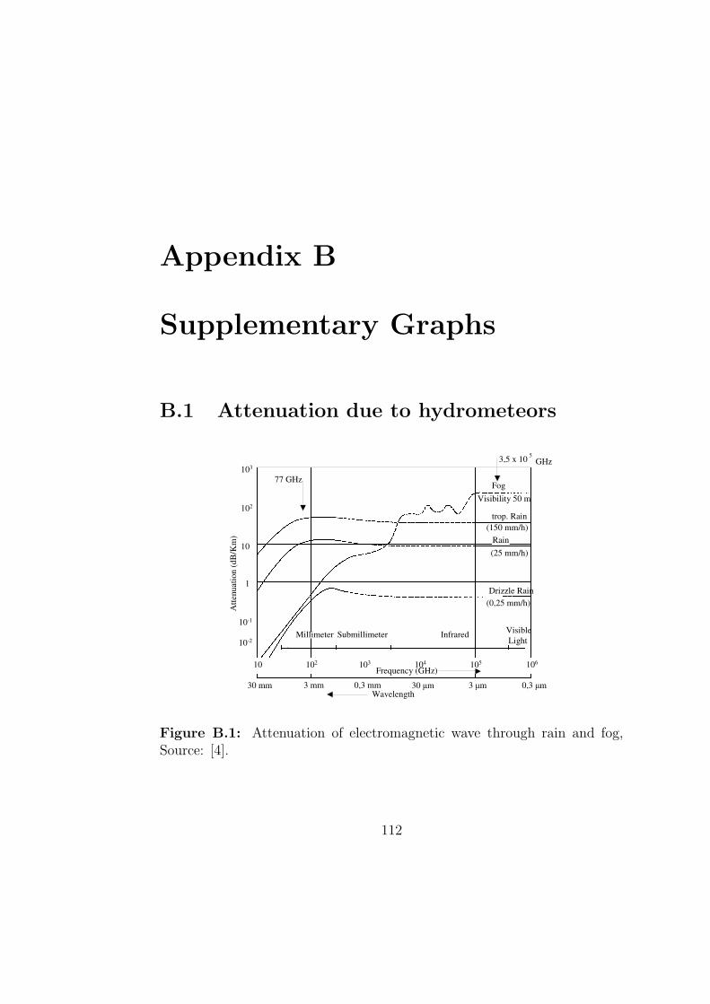
Appendix B
Supplementary Graphs
B.1 Attenuation due to hydrometeors
Wavelength
Atte
nuat
ion
(dB
/Km
)
Frequency (GHz)
103
102
10
10-1
10-2
10 102 103 104 105 106
3 mm30 mm 0,3 mm 30 µm 3 µm 0,3 µm
Millimeter Submillimeter Infrared VisibleLight
1
FogVisibility 50 m
trop. Rain(150 mm/h)
Rain(25 mm/h)
Drizzle Rain(0,25 mm/h)
77 GHz
3,5 x 10 5 GHz
Figure B.1: Attenuation of electromagnetic wave through rain and fog,Source: [4].
112
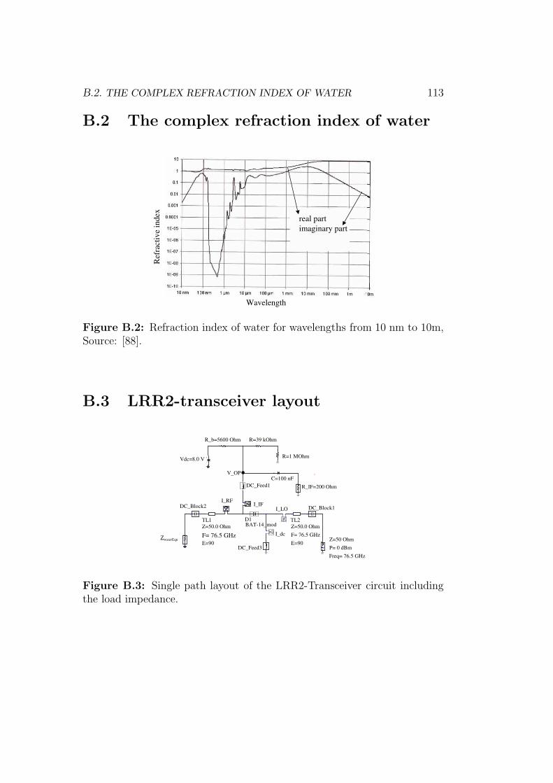
B.2. THE COMPLEX REFRACTION INDEX OF WATER 113
B.2 The complex refraction index of water
Wavelength
Ref
ract
ive
inde
x
real partimaginary part
Figure B.2: Refraction index of water for wavelengths from 10 nm to 10m,Source: [88].
B.3 LRR2-transceiver layout
V_OP
I_IF
I_dc
I_LOI_RF
DC_Feed1
TL1
F= 76.5 GHzE=90
Z=50.0 Ohm
DC_Block2
DC_Feed3
BAT-14_modD1
R_IF=200 Ohm
R_b=5600 Ohm
EqnVar
R=1 MOhm
R=39 kOhm
C=100 nF
ZwaterEqu
Freq= 76.5 GHzP= 0 dBmZ=50 Ohm
TL2
F= 76.5 GHzE=90
Z=50.0 Ohm
DC_Block1
Vdc=8.0 V
Figure B.3: Single path layout of the LRR2-Transceiver circuit includingthe load impedance.
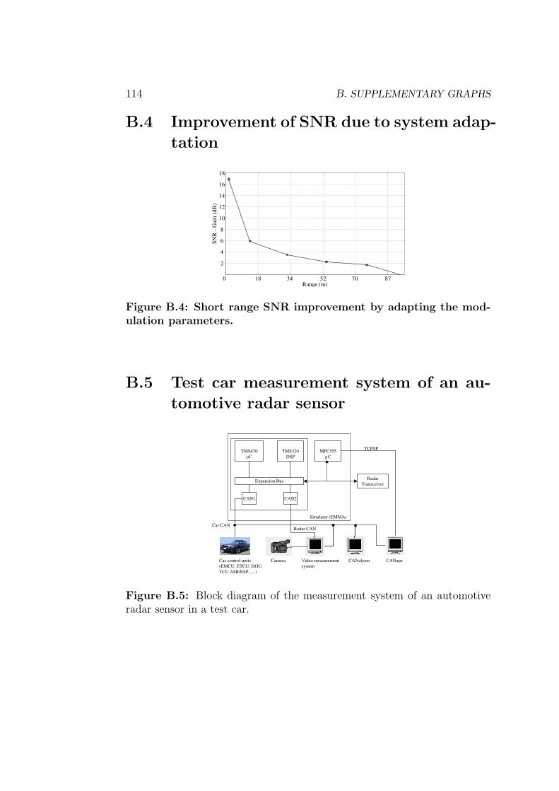
114 B. SUPPLEMENTARY GRAPHS
B.4 Improvement of SNR due to system adap-
tation
0 18 34 52 70 87
2
4
6
8
10
12
14
16
18
Range (m)
SNR
- G
ain
(dB
)
Figure B.4: Short range SNR improvement by adapting the mod-ulation parameters.
B.5 Test car measurement system of an au-
tomotive radar sensor
TMS470µC
TMS320DSP
Emulator (EMMA)
MPC555µC
Expansion Bus
CAN1 CAN2
Radar Transceiver
Car control units (EMCU, ETCU, DOU, TCU ASR/ESP, ... )
Camera Video measurementsystem
CANalyzer CANape
TCP/IP
Radar CANCar CAN
Figure B.5: Block diagram of the measurement system of an automotiveradar sensor in a test car.
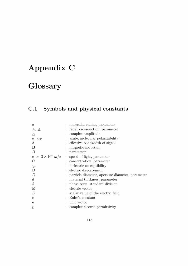
Appendix C
Glossary
C.1 Symbols and physical constants
a : molecular radius, parameterA, A : radar cross-section, parameterA : complex amplitudeα, αT : angle, molecular polarizabilityβ : effective bandwidth of signalB : magnetic inductionB : parameterc ≈ 3 × 10⁸ m/s : speed of light, parameterC : concentration, parameterχe : dielectric susceptibilityD : electric displacementD : particle diameter, aperture diameter, parameterd : material thickness, parameterδ : phase term, standard divisionE : electric vectorE : scalar value of the electric fielde : Euler’s constante : unit vectorε : complex electric permittivity
115
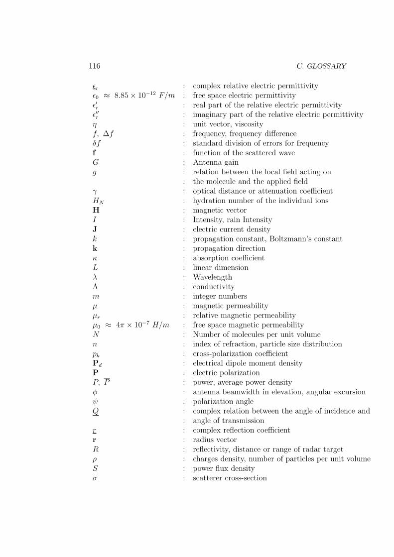
116 C. GLOSSARY
εr : complex relative electric permittivityε0 ≈ 8.85 × 10⁻¹² F/m : free space electric permittivityε′r : real part of the relative electric permittivityε′′r : imaginary part of the relative electric permittivityη : unit vector, viscosityf, ∆f : frequency, frequency differenceδf : standard division of errors for frequencyf : function of the scattered waveG : Antenna gaing : relation between the local field acting on
: the molecule and the applied fieldγ : optical distance or attenuation coefficientHN : hydration number of the individual ionsH : magnetic vectorI : Intensity, rain IntensityJ : electric current densityk : propagation constant, Boltzmann’s constantk : propagation directionκ : absorption coefficientL : linear dimensionλ : WavelengthΛ : conductivitym : integer numbersµ : magnetic permeabilityµr : relative magnetic permeabilityµ0 ≈ 4π × 10−7 H/m : free space magnetic permeabilityN : Number of molecules per unit volumen : index of refraction, particle size distributionpk : cross-polarization coefficientPd : electrical dipole moment densityP : electric polarizationP, P : power, average power densityφ : antenna beamwidth in elevation, angular excursionψ : polarization angleQ : complex relation between the angle of incidence and
: angle of transmissionr : complex reflection coefficientr : radius vectorR : reflectivity, distance or range of radar targetρ : charges density, number of particles per unit volumeS : power flux densityσ : scatterer cross-section
C.2. ABBREVIATIONS 117
t, ∆t : time, time differencet : complex transmission coefficientT : Transmissivity, period, absolute temperatureTm : modulation timeδTR : standard division of error for rangeτ : relaxation time, effective time duration of signaltan δ : loss tangentθ : antenna beamwidth in azimuthv, vr : velocity, relative velocityV, VRCR : Volume, rain cell volumew, dw : angular frequency, differential solid anglex, y, z : Cartesian coordinates
Z0 =√
µ0
ε0≈ 377 ohm : free space wave impedance
Z : wave impedance, meteorological reflectivity<> : statistical mean or average
C.2 Abbreviations
ACC : Adaptive Cruise ControlADC : Analog Digital ConverterAICC : Autonomous Intelligent Cruise ControlCM : Collision MitigationCWAS : Collision Warning and Avoidance SystemsCW : Continuous WaveDSP : Digital Signal ProcessingEM : ElectroMagneticFFT : Fast Fourier TransformationFMCW : Frequency Modulated Continuous WaveHPW : Half Power WidthIEEE : International Electrical and Electronics EngineeringMM-Wave : MilliMeter-waveMMIC : Microwave Monolithic Integrated CircuitNL : Nnumber of LayerNLE : Number of Linear EquationPLL : Phase Locked Loop
118 C. GLOSSARY
LRR2 : Long Range Radar second generationOP : Operation PointRCS : Radar Cross-SectionRF : Radio FrequencySNR : Signal-to-Noise RatioTE-Wave : Transversal Electric WaveTM-Wave : Transversal Magnetic waveVCO : Voltage Controlled OscillatorVNA : Vector Network AnalyzerVSWR : Voltage Standing Wave Ratio⊥, ‖ : perpendicular and parallel components of polarizations
Literature
[1] G. R. Wildmann, M. K. Daniels, L. Hamilton, L. Humm, B. Riley, J. K.Schiffmann, D. E. Schnelker and W. H. Wishon. Comparison of lidar-based and radar-based adaptive cruise control systems. SAE 2000 WorldCongress, March 6-9, 2000.
[2] Akira Ishimaru. Wave Propagation and Scattering in Randome Media,volume 1 and 2. Acadamic Press, New York, 1978.
[3] E. D. R. Shearman, E. G. Hoare and A Hutton. Trials of automotiveradar performance in road spray. IEE, 1998.
[4] J. Detlefsen. Radartechnik: Grundlagen, Bauelemente, Verfahren, An-wendungen. Springer - Verlag, Berlin, Heidelberg, 1989.
[5] E. F. Belohoubek. Radar control for automotive collision mitigation andheadway spacing. IEEE Trans. Veh. Technol., 31:89–99, May. 1982.
[6] E. Brus. Vehicular radar: The ultimate aid for defensive driving. Mi-crowaves & RF, pages 53–58, Sept. 1987.
[7] A. Kawakubo, S. Tokoro, Y. Yamada, K. Kuroda and T. Kawasaki.Electronically-scanning millimeter-wave radar for forward objects de-tection. 2004SAE International, pages 127–134, 2004.
[8] M. Born, E. Wolf. Principles of Optics. Cambridge University Press,Cambridge, 7th edition, 2003.
[9] Edward E. Altshuler. A simple expression for estimating attenuation byfog at millimeter wavelengths. IEEE Trans. on Antennas and Propaga-tion, AP-32:757–758, 1984.
119
120 LITERATURE
[10] Joseph Nemarich, Ronald J. Wellman, and James Lacombe. Backscatterand attenuation by falling snow and rain at 96, 140, and 225 ghz. IEEETrans. Geoscience and Remote Sensing, 26:319–329, May 1988.
[11] Takeshi Manabe, Toshio Ihara, and Jun Awaka. The relationship ofraindrop-size distribution to attenuations experienced at 50, 80, 140 and240 ghz. IEEE Tranc. on Antennas and Propagation, AP-35:1093–1096,November 1987.
[12] M. M. Z. Kharadly. Scattering by rain and melting snow. Antenna andPropagation, 2:406–410, 1989.
[13] Victor W. Richard, John E. Kammerer, and H. Bruce Wallace. Rainbackscatter measurements at millimeter wavelengths. IEEE Transactionon Geoscience and Remote Sensing, 26:244–252, May 1988.
[14] Matsuo Sekine, Chii-Dong Chen, and Toshimitsu Musha. Rain attenua-tion from log-normal and weibull raindrop-size distributions. IEE Trans.on Antennas and Propagation, AP-35:358–359, 1987.
[15] Alebel Arage, Goetz Kuehnle, Rolf Jakoby. Measurement of wet antennaeffects on millimeter wave propagation. 2006 IEEE Radar Conference,2006.
[16] Alebel Arage, Wolf M. Steffens, Goetz Kuehnle, Rolf Jakoby. Effectsof water and ice on automotive radar. German Microwave Conference,2006.
[17] American Institute of Physics. American Institute of Physics Handbook.McGraw-Hill, New York, 3rd edition, 1972.
[18] N. W. Ashcroft and N. D. Mermin. Solid State Physics. Holt, Rinehart,and Winston, New York, 1976.
[19] J. S. Blackemore. Solid State Physics. W. B. Saunders Co., Philadelphia,1974.
[20] A. R. von Hippel. Dielectrics and Waves. Wiley, New York, 1954.
[21] J. A. Saxton. Dielectric dispersion in pure polar liquids at very highradio-frequencies: Ii. relation of experiment results to theory. Proceed-ings of the Royal Society of London, Volume 213:473–491, 1952.
LITERATURE 121
[22] Simon Ramon, John R. Whinnery, Theodore Van Duzer. Fields andWaves in Communication Electronics, volume 2nd Edition. John Wileyand Sons, New York, Chichester, Brisbane, Toronto, Singapore, 1984.
[23] H. Frohlich. Theory of dielectrics. Clarendon Press, Oxford, 1949.
[24] H. Eyring. The Theory of rate processes. McGraw-Hill Book Co. Inc,New York, 1941.
[25] J. A. Lane and J. A. Saxton. Dielectric dispersion in pure polar liquidsat very high radio-frequencies: I. measurements on water, methyl andethyl alcohols. Proceedings of the Royal Society of London, 213:400–408,1952.
[26] W. J. Ellison, K. Lamkaouchi and J.-M. Moreau. Water: A dielectricreference. J. Mol. Liquids 68, pages 171–279, 1996.
[27] T. Meissner and F. J. Wentz. The complex dielectric constant of pureand sea water from microwave satellite observations. IEEE Trans.Geosci. Remote Sensing 42, pages 1836–1849, 2004.
[28] G. W. Robinson, S. -B. Zhu, S. Singh, and M. W. Evans. Water in biol-ogy, chemistry and physics: Experimental overviews and computationalmethodologies. World Scientific, Singapore, 1996.
[29] Jonathan H. Jiang and Dong L. Wu. Ice and water permittivity formillimeter and sub-millimeter remote sensing applications. AtmosphericScience Letters, March 31, 2004.
[30] H. Mayer. Physik Dunner Schichten, volume Band 4, Teil 1. Wiss.Verlag Ges. M. B. H., Stuttgart, 1950.
[31] Eugene Hecht, Adelphi University. Optics, Second Edition. Addison-Wesley Publisching Company, Reading, Massachusetts, 1987, 1974.
[32] R. S. Longhurst. Geometrical and Physical Optics. Longman Scientificand Technical Group, England, 3rd edition, 1993.
[33] Peter Beckmann, Andre Spizzichino. The Scattering of ElectromagneticWaves from Rough Surfaces. Pergamon Press LTD., Oxford, London,New York, Paris, 4 edition, 1963.
122 LITERATURE
[34] Milton Kerker. The Scattering of Light. Acadamic Press, Inc., NewYork, 1969.
[35] H. Gent, I. M. Hunter and N.P. Robinson. Polarization of radar echoes,including aircraft, precipitation and tarrain. Proc. IEE, 110:2139–2148,December 1963.
[36] Akira Ishimaru. Electromagnetic Wave Propagation, Radiation, andScattering. Prentice-Hall, Inc., New Jersey, 1991.
[37] R. L. Cosgriff, W. H. Peake, R. C. Tayor. Terrain Scattering Propertiesfor Sensor System Design. Engineering Experiment Station, The OhioState University, Columbus, 1959.
[38] S. Silver. Microwave Antenna Theory and Design. McGraw-Hill, NewYork, 1949.
[39] M. I. Skolnik. Radar Systems, volume 2nd Edition. McGraw-Hill, Inc.,New York, 1962.
[40] G. Kuhnle, H. Mayer, H. Olbrich, W. Steffens and H. C. Swoboda.Low-cost long-range radar for future driver assistance systems. AutoTechnology, November 2003.
[41] M. I. Skolnik. Introduction to Radar Systems. McGraw-Hill, Inc., NewYork, 1980.
[42] John Gowar. Optical Communication System. Prentice Hall Europ,Trowbridge, Wiltshire, U.K., 2nd edition, 1993.
[43] Siemens AG: G. Mahlke, P. Goessing. Lichtwellenleiterkabel, volume 4.MCD Verlag, Erlangen, 1995.
[44] Reinhard Hammel. Zur Entfernungsauflosung von Punktzielen mitFMCW-Radarsystemen. DLR-Forschungsbericht 89-47, 1989.
[45] Klaus Peter Wagner. Winkelauflosende Radarverfahren fur Kraft-fahrzeuganwendungen. Dessertation, Munchen, 1997.
[46] Alebel Arage. Entwicklung und Verifikation von Moglichkeiten zurDegradationserkennung bei Adaptive-Cruise-Control (ACC)- Radarsen-soren. M. SC. Thesis, Darmstadt, 2003.
LITERATURE 123
[47] Ramzi Abou-Jaoude. Acc radar sensor technology, test requirements,and test solutions. IEEE Trans. on Intelligent Transportation Systems,4:115–122, September 2003.
[48] Rudolf Kuehn. Mikrowellen Antennen. VEB Verlag Technik, Berlin,1964.
[49] I. J. Bahl, P. Bhartia. Microstrip Antennas. Artech House, Inc, Massa-chusetts, 1980.
[50] J. Brown. Microwave Lenses. Methuen and CO. LTD., London, 1stedition, 1953.
[51] Richard C. Johnson. Antenna Engineering Handbook, volume 3rd.McGraw-Hill Inc., New York, 1993.
[52] K. L. Fuller. To see and not to be seen. IEE Proc.-F, Comun., Radar& Signal Process., 137:1–10, 1990.
[53] Jerry L. Eaves, Edward K. Reedy. Principles of Modern Radar. VANNostrand Reinhold Company, New York, 1987.
[54] A. G. Stove. Linear fmcw radar techniques. IEE Proc.-F,, 139:343–350,October 1992.
[55] T. V. Kerssenbrock, P. Heide. Novel 77 ghz flip-chip sensor modules forautomotive radar applications. IEEE MTT-S International MicrowaveSymposium, June 13-19, 1999.
[56] L. Raffaelli. Millimeter-wave automotive radars and related technology.IEEE MTT-S Digest, pages 35–37, june 1996.
[57] J. Robinson, D. K. Paul, J. Bird, D. Dawson, T. Brown, D. Spencer,and B. Prime. A millimeteric car radar front end for automotive cruisecontrol. IEE, 9:1–8, 1998.
[58] B. C. Blevis. Losses due to rain and radomes and antenna reflectingsurfaces. IEEE Trans. on antennas and propagation, pages 175–176,Ap. 13, 1965.
124 LITERATURE
[59] M. R. Islam, A. R. Tharek. Wet antenna effects on microwave propa-gation - an overview and results from sprayer tests. Proceeding of In-ternational Wireless Telecommunication Symposium, pages 94–97, May17-20, 2000.
[60] G. Liu, J. T. Ong, E. Choo, and C. G. Teo. Techniques to separate wetradome loss from measured rain attenuation data during rain events.IEE:Electronics Letters, 36:904–906, 11th May 2000.
[61] Carlo G. Someda. Electromagnetic Waves: Optoelectronics Imaging andSensing, volume Series Edition. Chapman and Hall, London, Weinheim,New York, Tokyo, Melbourne, Madras, 1998.
[62] Horst Wupper. Grundlagen Elektronischer Schaltungen. Dr. AlfredHuethig Verlag, Heidelberg, 2nd edition, 1986.
[63] M. R. Islam, A. R. Tharek, J. Din, J. Chebil. Measurement of wetantenna effects on microwave propagation - an analytical approach. Mi-crowave Conference, pages 1547–1551, Dec. 3-6, 2000.
[64] Anritsu. Series 371xxA Vector Network Analyzer Operational Manual.Anritsu Co., Morgan Hill, California, 1997.
[65] K. Lange, K.-H. Lochrer. Taschenbuch der Hochfrequenztechnik.Springer-Verlag, Berlin, 5 edition, 1992.
[66] Martin Nilsson. Water-induced charge transport in microcrystalline cel-lulose. 2006.
[67] Serka Fernandez. Dielectric relaxation study of the cellulose solvent sys-tem LICl/N,N-dimethylacetamide. Dessertation, Regensburg, 2003.
[68] R. Raffaelli, M. Tedesco, C. Riminesi and A. Ignesti. Thickness-independent measurement of the permittivity of thin samples in thex band. IOP Publishing Ltd, UK, pages 503–509, 28 February 2002.
[69] P. Bhartia, I. J. Bahl. Millimeter Wave Engineering and Applications.John Wiley & Sons, Inc., New York, 1984.
[70] Peter A. Rizzi. Microwave Engineering: Passive Circuits. Prentice-Hall,Inc., New Jersey, 1988.
LITERATURE 125
[71] Stephen A. Mass. Microwave Mixers, volume 2nd. Artech House,Boston, 1993.
[72] Zinke, Brunswig. Hochfrequenztechnik 2, 5.Auflage, Herausgegeben vonA. Vlcek, H.L. Hartnagel und K. Mayer. Springer-Verlag, Berlin, Hei-delberg, 5th edition, 1999.
[73] H. William. Numerical Recipes. Cambridge University Press, Cam-bridge, 2nd edition, 1992.
[74] Fred E. Nathanson, J. Patrick Reilly, Marvin N. Cohen. Radar DesignPrinciples, volume 2nd. McGraw-Hill, Inc., New York, 1990.
[75] F. B. Dyer, N. C. Currie, and M. S. Applegate. Radar backscatterfrom land, sea, rain, and snow at millimeter wavelengths. InternationalConference Radar 77, pages 559–563, 25-28 Oct. 1977.
[76] Julius Goldhirsh. Prediction methods of rain attenuation statistics atvariable path angles and carrier frequencies between 13 and 100 ghz.IEEE Trans. on Antennas and Propagation, AP-23:786–791, November,1975.
[77] Joerg Sander. Rain attenuation of millimeter waves at wavelebgth of5.77, 3.3, and 2 mm. IEEE Trans. on Antennas and Propagation, AP-23:213–220, 1975.
[78] Charles E. Hendrix, Gregory Kulon, and Thomas A. Russell. Specifi-cation of Polarization Parameters for Optimal-Performance in Rain ofDual Circularly Polarized Radio Links, volume 40. May 1992.
[79] TA-Shing Chu. Frequency dependence of microwave depolarization ver-sus rain attenuation. IEEE Trans. on Antennas and Propagation, AP-32:994–997, September 1984.
[80] Wolfhard J. Vogel. A terrestrial rain depolarization compensation ex-periment at 11.7 ghz. IEEE Trans. on Communications, COM-31:1241–1246, November 1983.
[81] H. W. Arnold. Measurements and prediction of the polarization depen-dent properties of rain and ice depolarization. IEEE Trans. on Commu-nications, COM-29:710–715, May 1981.
126 LITERATURE
[82] J. Alfred, Jr. Bogush. Radar and the Atmosphere. Artech House, Inc.,MA, 1989.
[83] K. L. S. Gunn and T. W. R. East. The microwave properties of percip-itation particles. Journal of the Royal Meteorol Society, pages 523–545,1954.
[84] Robert Schneider. Modellierung der Wellenausbreitung fur ein bildgeben-des Kfz-Radar. Dissertation, Karlsruhe, 1998.
[85] I. Anderson. Measurements of 20 ghz transmission through a radome inrain. IEEE Trans., AP-23:699–622, Sptember 1975.
[86] A. Cohen, and A. Smolski. The effect of rain on satellite communicationsearth terminal rigid radomes. Microwave J., 9:111–121, September 1966.
[87] R. M. Weigand. Performance of a water-rapellent radome coating in anairport surveillance radar. IEEE Proc., 61:1167–1168, September 1973.
[88] D. J. Segelstein. The complex refractive index of water, in physics.University of Missouri, Kansas City, 1981.
List of published papers
• Alebel Arage, Gotz Kuhnle, Rolf Jakoby, ”Measurement of Wet An-tenna Effects on Millimeter Wave Propagation”, 2006 IEEE RADARConference, Verona, USA, 2006.
• Alebel Arage, Wolf Steffens, Gotz Kuhnle, Rolf Jakoby, ”Effects ofWater and Ice Layer on Automotive Radar”, German Microwave Con-ference (GeMiC) 2006, University of Karlsruhe, Germany, 2006.
• Alebel Arage, Wolf Steffens, Joachim Hauk, Gotz Kuhnle, Rolf Jakoby,”Identification of Wetness on Millimeter Wave Radar Surface”, Fre-quenz: Journal of RF-Engineering and Telecommunications, vol. 60,2006, pp. 28-30.
• Alebel Arage, Jorg Hilsebecher, Joachim Hauk, ”Messung der Reflexionan einem Linsen- /Radomsystem mit Slow Speed- FSK-Modulationssystem”, Robert Bosch GmbH, September 2005.
List of submitted patents
• Alebel Arage, Jorg Hilsebecher, Juachim Hauk, ”Messung der Re-flexionsstarke an der Linsen- / Radomoberflache durch Mischerarbeit-spunktverschiebung”, Patentschrift: Patent Application No. 2005/0932,date of filing 16.03.2005.
• Alebel Arage, ”Erkennung und Messung der Niederschlagsintensitatmit Automotive Long Range Radar-System”, Patentschrift: PatentApplication No. 2005/2423, date of filing 21.07.2005.
• Alebel Arage, Klaus Lehre, Klar Michal, Jorg Hilsebecher, ”Frequenz-Scanning Verfahren zur Messung der Reflexion an der Linsen- / Radombele-gung”, Patentschrift: Patent Application No. 2006/0315, date of filing20.01.2006.
Comment on my participation: experiments, analysis, planning, writing

Curriculum Vitae
Personal Information:
Name Alebel Arage HassenDate & Place of Birth 27th December 1970 in Woreillu, Ethiopia
Education:
09.1976 - 06.1980 Worillu Elementary School, Ethiopia09.1981 - 04.1986 Woreillu Secondary school, EthiopiaApril 1986 GEC Level ”A”01.1987 - 12.1988 Associate Degree in Electro-Mechanics, Electrical and
Electronics Institute, Addis Ababa, Ethiopia04.1995 - 10.1999 B. SC. in Electrical Engineering and Information
Technology, Institute of Applied Science,Giessen, Germany
04.2000 - 06.2003 M. SC. in Communication Engineering,Technical University of Darmstadt, Germany
Work Experience:
01.1989 - 08.1993 Technical Expert, Ethiopia Electric Light and PowerAuthority (EELPA), Addis Ababa, Ethiopia
02.1998 - 12.1999 Technical Trainee, Siemens AG, Munich, Germany11.1999 - 12.2000 Software Developer, Siemens AG, Frankfurt a.M.,
Germany01.2001 - 09.2001 Software Developer, Web Arts AG, Friedrichsdorf,
Germany01.2002 - 06.2002 Software Developer, Daimler Chrysler AG,
Frankfurt a.M., Germany11.2002 - 09.2006 Researcher, Robert Bosch GmbH, Leonberg, Germany