increased genomic prediction accuracy in wheat … increased genomic prediction accuracy in wheat...
TRANSCRIPT
1
Increased Genomic Prediction Accuracy in Wheat Breeding Through Spatial Adjustment 1
of Field Trial Data 2
3
Bettina Lado*, Ivan Matus§, Alejandra Rodríguez§, Luis Inostroza§, Jesse Poland†, François 4
Belzile‡, Alejandro del Pozo**, Martín Quincke* and Jarislav von Zitzewitz§§,1 5
6
*Programa Nacional de Investigación Cultivos de Secano, Instituto Nacional de investigación 7
Agropecuaria, Est. Exp. La Estanzuela, Colonia 70000, Uruguay, §Instituto de Investigaciones 8
Agropecuarias, Centro Regional de Investigación Quilamapu, Casilla 426, Chillán, Chile, 9
†United States Department of Agriculture, Agricultural Research Service, Hard Winter Wheat 10
Genetics Research Unit, Manhattan, Kansas and Department of Agronomy, Kansas State 11
University, Manhattan, Kansas, United States of America, ‡Département de Phytologie and 12
Institut de biologie intégrative et des systèmes (IBIS), Université Laval, Québec, QC, Canada, 13
**Universidad de Talca, Facultad de Ciencias Agrarias, Casilla 747, Talca, Chile, §§SECOBRA 14
Saatzucht GmbH, Feldkirchen 3, 85368 Moosburg, Germany 15
16
1 Corresponding author: Jarislav von Zitzewitz 17
email: [email protected] 18
19
20
21
G3: Genes|Genomes|Genetics Early Online, published on September 30, 2013 as doi:10.1534/g3.113.007807
© The Author(s) 2013. Published by the Genetics Society of America.
2
22
Wheat Genomic Selection 23
24
Key words: Genotyping-by-sequencing, Genomic Selection, Wheat, Single Nucleotide 25
Polymorphism, Quantitative Trait Locus, Spatial Correction, GBLUP. 26
27
28
Corresponding author's name: Jarislav von Zitzewitz 29
Address: SECOBRA Saatzucht GmbH, Feldkirchen 3, 85368 Moosburg, Germany 30
31
32
33
34
35
36
37
38
3
39
ABSTRACT 40
In crop breeding, the interest of predicting the performance of candidate cultivars in the field has 41
increased due to recent advances in molecular breeding technologies. However, the complexity 42
of the wheat genome presents some challenges for applying new technologies in molecular 43
marker identification with Next Generation Sequencing (NGS). We applied “Genotyping-by-44
Sequencing” (GBS) to identify single nucleotide polymorphisms (SNPs) in the genomes of 384 45
wheat (Triticum aestivum) breeding lines that were field tested under three different water 46
regimes in Mediterranean climatic conditions: rainfed, mild water stress, and fully irrigated. We 47
identified 102,324 SNPs in these lines, and the phenotypic data were used to train and test 48
genomic selection models intended to predict yield, thousand-kernel weight, number of kernels 49
per spike and heading date. Phenotypic data showed marked spatial variation. Therefore, 50
different models were tested to account for observed field trends. A mixed-model using moving-51
means as a covariate was found to best fit the data. When applying the genomic selection 52
models, the accuracy of predicted traits increased with spatial adjustment. Multiple genomic 53
selection models were tested and a Gaussian kernel model was determined to give the highest 54
accuracy. The best predictions between environments were obtained when data from different 55
years were used to train the model. Our results confirm that GBS is an effective tool to obtain 56
genome-wide information for crops with complex genomes, that this data is efficient for 57
predicting traits, and that correction of spatial variation is a crucial ingredient to increase 58
prediction accuracy in genomic selection models. 59
60
4
61
INTRODUCTION 62
Wheat is among the most important cereal crops in the world, with a total production of 650 - 63
700 million tons annually (FAOSTAT, 2011). In order to meet future demands of growing global 64
populations, one of the most important breeding objectives is increasing total yields while 65
adapting to new and changing environments. 66
New genomic tools in wheat breeding have allowed the incorporation of new allelic variants into 67
adapted germplasm. Strategies like quantitative trait loci (QTL) and association mapping have 68
aided in identifying genes or genomic regions responsible for traits of interest (Lander and 69
Botstein 1989; Jansen 1993; Tanksley 1993; Risch and Merikangas 1996; Pritchard 2000; 70
Kraakman et al. 2004; Kirigwi et al. 2007; Neumann et al. 2010; LeGouis et al. 2012; Yu et al. 71
2012). Trait associated markers then become selection targets to assist in molecular breeding 72
programs (Collard et al. 2005; Landjeva et al. 2007; Collard and Mackill 2008; Buerstymayr et 73
al. 2009). However, these approaches have limitations due to the difficulty in detecting 74
significant markers within gene regions that are involved in the expression of complex traits 75
influenced by many genes at different levels (Xu 2003) as well as accurately modeling gene 76
effects directly in breeding germplasm and target environments. The most important traits 77
involved in breeding are complex. Therefore, other strategies that take into account thousands of 78
makers at one time in a model to predict complex traits have recently been developed. 79
Genomic Selection (GS) is a recent approach being applied in crop breeding to make decisions 80
for advancing germplasm from one generation to the next. GS was first proposed in animal 81
5
breeding by Meuwissen et al. (2001). The development of high-throughput sequencing 82
platforms, yielding a vast amount of information for each breeding line, allows the application of 83
GS. In order for GS to be applicable in commercial breeding, genotyping methods need to be 84
cost effective. Genotyping-by-Sequencing (GBS) is a high throughput genotyping method that 85
has been shown to be very useful for complex genomes like wheat (Poland et al. 2012a; Poland 86
and Rife 2012). GBS costs are directly linked to the decreasing cost of sequencing driven by 87
global research into developing new low-cost sequencing technologies and platforms. The wheat 88
genome is very large with 16 Gb (five times the human genome) and very complex with 80% 89
repeated regions and 25% to 30% of its genes duplicated (Bennett and Smith 1976; Dubcovsky 90
et al. 1996; Akhunov et al. 2003). Furthermore, wheat is a hexaploid species with 3 genomes (A, 91
B and D) per chromosome (Sarkar and Stebbins 1956; Dvorak and Zhang 1990; Dvorak et al. 92
1993). For effective reduction of these genomes, GBS uses methylation sensitive enzymes, 93
which results in the elimination of most of the repeated regions and reduces the genome 94
representation to increase the efficiency of sequencing (Elshire et al. 2011; Sonah et al. 2013). 95
The development of novel statistical approaches for GS is a crucial step, where all the genotypic 96
information is taken into account to be associated with phenotypic data, by adjusting the 97
parameters in a prediction model. The parameters of the model are currently being adjusted with 98
linear models (Ridge Regression), Bayesian approaches (Bayes A and Bayes B) and semi-99
parametric strategies (Reproducing Kernel Hilbert Spaces (RKHS) and neural networks) 100
(Meuwissen et al. 2001; Gianola et al. 2003; de los Campos et al. 2010; Endelman 2011; 101
Gianola et al. 2011; Goddard et al. 2011; Poland et al. 2012b). RKHS is defined by a 102
‘reproducing kernel’, which is a function of the relationship between pairs of genotypes. RKHS 103
is a semi-parametric approach, which could be represented as a parametric model by choosing 104
6
the appropriate kernel (De los Campos et al. 2010). Two kernels that are commonly applied are 105
known as Ridge Regression (RR) and Gaussian (GAUSS). The relationships between genotypes 106
in RR are established using an additive model, and in GAUSS, the relationship between 107
individuals are calculated with Euclidean distances that take into account epistatic interactions 108
(Gianola and van Kaam 2008; Endelman 2011). 109
As genotyping is taking a more routine and accepted approach, improvements in model 110
predictions are focused on precision phenotyping. Physiological differences and environmental 111
conditions that affect the precision of the measured phenotype, need to be taken into account in 112
order to have an accurate GS prediction model. The breeder needs to know with accuracy the 113
fields where selections will occur; therefore high-throughput phenotyping technologies are being 114
implemented prior to planting (characterization of field heterogeneity) and during crop 115
development to help reduce non-genetic variation (Crossa et al. 2006; Cabrera-Bosquet et al. 116
2012; Masuka et al. 2012; White et al. 2012). Field design can be applied that will help account 117
for the spatial variation, and model correction mechanisms that take into account field 118
heterogeneity that produces spatial correlation errors. These spatial trends can be eliminated 119
using post data treatment. There are different strategies, which include model variance-120
covariance matrixes, row-columns, and moving-means (Cullis et al. 1998; Peiris et al. 2008; 121
Müller et al. 2010; Leiser et al. 2012). 122
The objectives of this study were a) to validate the GBS technology as a tool for genotyping 123
germplasm with complex genomes; and b) to create an optimized training model for GS with a 124
germplasm to be bred in a Mediterranean climate environment of central Chile, using a diverse 125
set of wheat genotypes. Our study confirms that GBS is an inexpensive, robust, and useful tool to 126

7
obtain genomewide information for breeding programs that work with complex genomes, such 127
as wheat. Furthermore, we evaluate that spatial adjustment of the phenotypic data in each trial is 128
very important to reduce error in the model and increase prediction accuracy. Here we evaluate 129
spatial variation across the field, while also exploring fundamental variations that take into 130
account environmental and genotypic interactions. 131
MATERIALS AND METHODS 132
Germplasm and growth conditions: 133
The germplasm consists of 384 advanced lines from two different breeding programs including 134
55 lines from the wheat breeding program at Instituto Nacional de Investigación Agropecuaria 135
(INIA) in Chile, 143 from the International Wheat and Maize Improvement Centre (CIMMYT) 136
that were previously selected for adaptation to Chilean environments (these lines share common 137
ancestors with the INIA-Chile breeding program), and 186 lines from the Instituto Nacional de 138
Investigacion Agropecuaria (INIA) in Uruguay. The objective with this set of lines was to create 139
a germplasm base to breed for drier areas in Chile, and subsequently other countries in the 140
region. 141
The breeding germplasm was evaluated in the Mediterranean environment Santa Rosa (36º32’ S, 142
71°55’ W; 217 m.a.s.l.) under two levels of water supply, mild water stress (MWS) and fully 143
irrigated (FI), in 2011. In 2012 the lines were evaluated in Santa Rosa under the two levels of 144
water supply, and additionally evaluated in Cauquenes (35º 58’S; 72º 17’W), a traditionally dry-145
land agricultural region with lower yield potential. Cauquenes has a granitic soil (Alfisol) with 146
low fertility; the minimum average temperature is 4.7 ºC (July), the maximum 27 º C (January) 147
and the long-term average annual precipitation is 695 mm. Santa Rosa has a volcanic soil 148
8
(Andisol) with adequate fertility for wheat; the minimum average temperature is 3.0 ºC (July), 149
the maximum 28.6 º C (January) and long-term average annual precipitation is 1270 mm (del 150
Pozo and del Canto 1999). 151
The experimental design was an alpha-lattice with 20 incomplete blocks, each block containing 152
20 genotypes. Two replicates were used at both trials of Santa Rosa in 2011 and 2012, and at 153
Cauquenes in 2012. Plots consisted of five rows of 2 m long and 0.2 m distance among rows. 154
Sowing dates were on the 31st of August and 7th of September, at Santa Rosa and Cauquenes, 155
respectively and sowing rate was 20 g m2. Plots were fertilized with 260 kg ha-1 of ammonium 156
phosphate (46% P2O5 and 18% N), 90 kg ha-1 of potassium chloride (60% K2O), 200 kg ha-1 of 157
sulpomag (22% K2O, 18% MgO and 22% S), 10 kg ha-1 of boronatrocalcita (11% B) and 3 kg 158
ha-1 of zinc sulphate (35% Zn). At tillering stage an additional 80 kg ha-1 of N was applied. 159
Weeds were controlled with 2-methyl-4-chlorophenoxyacetic acid (MCPA) at 750 g a.i. ha-1 + 160
Metsulfuron Metil 8 g a.i. ha-1. Furrow irrigation was used at Santa Rosa: one irrigation (at 161
tillering) for the MWS trial and four irrigations (at tillering, flag leaf emergence, heading and 162
mid-grain filling) of ca. 50 mm each for the FI trial. 163
For phenotyping, all lines were evaluated for grain yield (GY), thousand kernel weight (TKW), 164
number of kernels per spike (NKS) and days to heading (DH) in 2011. In 2012, only GY was 165
evaluated. For the yield components (TKW and NKS), 25 spikes were randomly selected from 166
each plot. For GY the whole plot was harvested. DH was recorded as the number of days from 167
sowing till 50% of spikes emerged. 168
SNP identification: 169
9
Genomic DNA was extracted using DNeasy Plant Maxi Kit® (Qiagen). Library construction was 170
followed by using the PstI-MspI genotyping-by-sequencing (GBS) protocol described by Poland 171
et al. (2012a). This step and sequencing was performed twice. The libraries were made in 172
collaboration with the Kansas State University (KSU), USA, and the Institut de Biologie 173
Intégrative et des Systèmes (IBIS) at Université Laval, Quebec, Canada. The sequencing was 174
performed on an Illumina® Hi-Seq 2000 at the sequence facility at the DNA core facility at the 175
University of Missouri (USA) and the McGill Univesity-Génome Quebec Innovation Centre 176
(Montreal, Canada) for each set of libraries. The sequences were analyzed, in relation to base 177
quality and distribution of sequence in different samples, using the Galaxy® 178
(http://galaxy.psu.edu/) software. 179
SNP calls were made using the Tassel Pipeline (TP) (http://maizegenetics.net), with modification 180
for non-reference SNP calling by Poland et. al. (2012a). The TP handles the sequence 181
information coming from next-generation sequencing. Tags are defined, which are a set of 182
identical sequences, and then the number of sequences per tag are counted. Tags with less than 183
15 reads across were filtered to remove low frequency tags resulting from sequencing errors. 184
Tags are then defined individually by the lines that it came from. A pairwise alignment between 185
tags to call some set of potential SNPs is then established. The TP has different filters for calling 186
SNPs. In this study inbred lines that are in a highly homozygous state were used, therefore the 187
‘inbreeding coefficient’ filter was used and set to 0.9 to eliminate SNPs with high amount of 188
heterozygous calls resulting from alignment of paralogs and duplicate sequences. The minor 189
allele frequency filter was set to 0.01, and minimum locus coverage was set to eliminate SNPs 190
with more than 80% missing data. Once the complete SNP matrix was established (Supplemental 191
data), the missing data was imputed using the realized relationship matrix method (MVN-EM) 192
10
describing by Poland et al. (2012b) with the R environment (R Core Team, 2013) package 193
rrBLUP (Endelman 2011). In order to further verify that the imputed SNPs had not affected, the 194
genetic relationship matrix we correlated with and without imputed SNPs. Then, to further verify 195
the quality of the imputed SNPs, marker-based kinship matrixes between random subsets of 196
SNPs were calculated and compared using the package ‘rrBLUP’ (Endelman 2011). 197
Genetic and phylogenetic comparisons: 198
SNP data from 384 diverse wheat genotypes were used to calculate the kinship (A) matrix of 199
genotypes using the EMMA package (Kang et al. 2008) in R environment (R Core Team, 2013). 200
The dissimilarity matrix (1 - similarity matrix) was analyzed by principal coordinate analysis 201
(PCoA) using ape package (Paradis et al. 2004) in R. 202
Sequence alignments: 203
The SNP tags were BLASTed against the sequence database available from the Synthetic x 204
Opata map by Poland et al. (2012a) (available at 205
http://www.wheatgenetics.org/index.php/download/viewcategory/10-synop) using blastn from 206
package ncbi-blast+ (Altschul et al. 1990) setting the parameters, maximum target and number 207
of threads in 1, and percent of identity at 95 %. 208
Linkage Disequilibrium (LD) between each pair of mapped SNPs was calculated as R2 using the 209
trio package (Schwender et al. 2012) in R. SNPs were ordered following the bin map order 210
presented by the Poland et al. (2012a) database. After SNPs were ordered, the LD values were 211
plotted using the LDheatmap package (Shin et al. 2006) in R. 212
Phenotypic predictions: 213
11
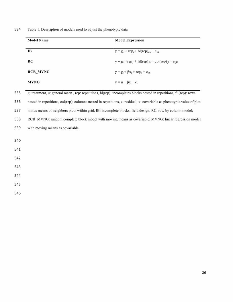
Phenotypic data was analyzed using the lme4 (Bates 2007) and mvngGrAd (Technow 2012) 214
packages in R. The analysis was performed individually for each condition and year. Two 215
different mixed models (in addition to field design model that was incomplete blocks), and one 216
linear regression model (Table 1) defined as Row-by-Column (RC), Random Complete Block 217
model with moving means (RCB_MVNG) and linear regression model with moving means as 218
covariable (MVNG), were considered to account for spatial correlations. Two of the four models 219
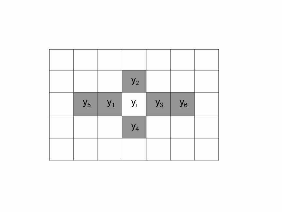
use a covariable to correct for spatial variation in the field. The covariable (xi) was calculated as 220
the value of phenotypic plot minus mean phenotypic value of neighbors plots, xi = yi – mean (y1, 221
y2, y3, y4, y5, y6) (Figure 1). 222
The three mixed models have a general expression as: 223
y = βX + Zu + e 224
where: X is the design matrix for fixed effects β, Z is the design matrix for random effects u 225
and e is the residual matrix that follows the distribution e ~ N(0,σe2I). After the analysis of the 226
residuals from each phenotypic model was established, the BLUPs were obtained to calculate 227
genomic predictions by Genomic Best Linear Unbiased Predictor (GBLUP) using the rrBLUP 228
package with two different kernels, RR and GAUSS (Endelman 2011).The predictions were 229
validated with 100 replications using the cross validation method described by Crossa et al. 230
(2010). The samples were sub-divided in 7 similar sets. The training population was composed 231
of six of the sets (86% of the samples) and the validation was done on the remaining set (14% of 232
the samples). For predictions between environments adjusted data from two environments were 233
used to train predictions in the remaining three environments. 234
RESULTS 235
12
SNP identification: 236
GBS SNPs were identified, among sequences tag pairs by allowing one to three mismatches 237
between tags. Two library replicates for the 384 samples were analyzed jointly, with a total of 238
102,324 SNPs identified. Similarities matrixes calculated with and without imputation showed 239
high correlation (r= 0.990, p-value<0.001). 240
Genetic and phylogenetic comparisons: 241
To test the predictability of the markers in constructing a genetic relationship matrix, the 102,324 242
SNPs were divided into two randomly assigned sets of 51,162 SNPs in each group. Two genetic 243
similarity matrices were constructed independently with each of the sets of SNPs. The Pearson 244
correlation between matrices was 0.997 (p-value = 0.001). A genetic similarity matrix was 245
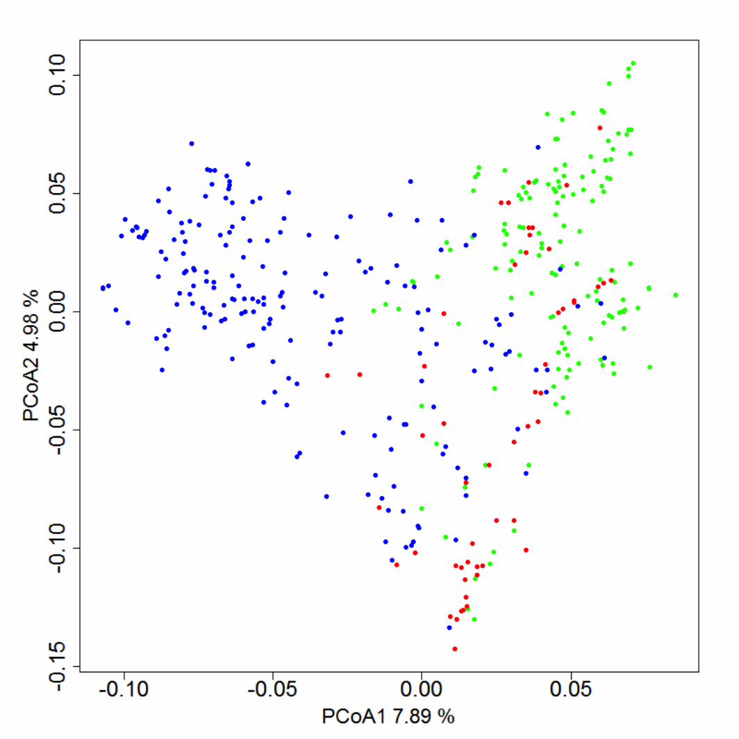
calculated with the complete set of markers to perform a principal coordinate analysis (Figure 2). 246
The germplasm was separated in two groups, representing each breeding program (CIMMYT-247
INIA Chile and INIA Uruguay). The first two principal coordinates explained 12.9 % of 248
variation. 249
Sequence alignments: 250
When comparing sequences using BLAST against the Poland et al. (2012a) GBS-based SNP 251
database, the sequences in common showed a good coverage throughout all 21wheat linkage 252
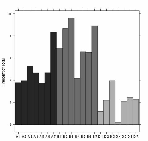
groups. Of all the SNPs, 13 % (13,357) found high quality matches. Although a good coverage 253
was observed, the D genome presented fewer SNPs than the A and B genomes (Figure 3). As 254
expected, linkage disequilibrium (LD) analysis between mapped SNPs indicated high LD 255
between closely linked SNPs along all chromosomes (Supplemental data). 256
13
Phenotypic analysis: 257
Phenotypic data was collected under different soil water availability in 2011 and 2012. The traits 258
under study (GY, TKW, NKS, DH) were analyzed adjusting for field design and for spatial 259
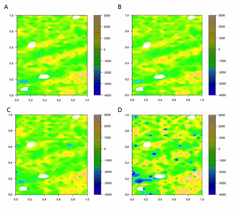
variation using linear mixed models. The residuals for the adjusted traits in 2011 were 260
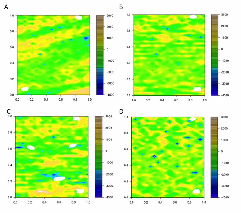
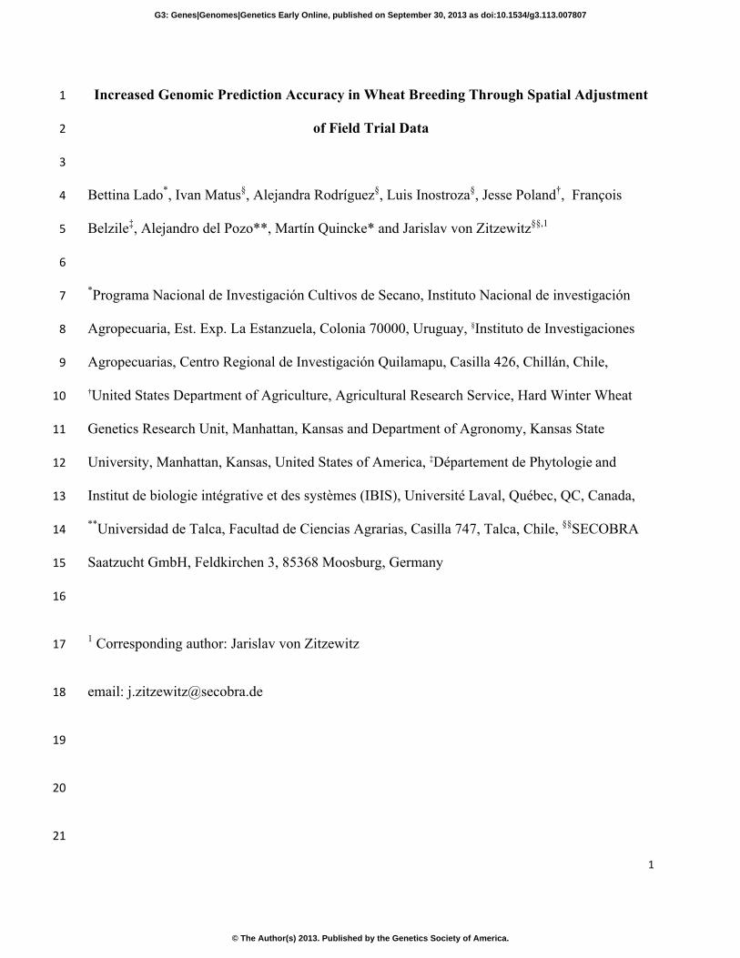
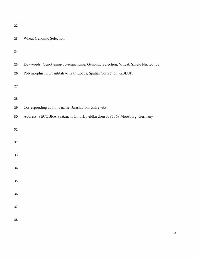
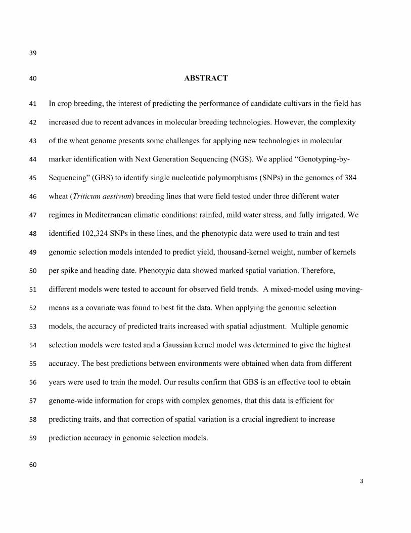
heterogeneous due to spatial correlations (Figure 4 and Figure 5). Other models (RC, 261
RCB_MVNG and MVNG) were considered to reduce correlations between residuals. The RC 262
model was inadequate to correct the residual heterogeneity because the same spatial correlation 263
was observed (Figure 4 and Figure 5). The other two (RCB_MVNG and MVNG) models, which 264
include a moving means as a covariable, better accounted for spatial variance as observed by 265
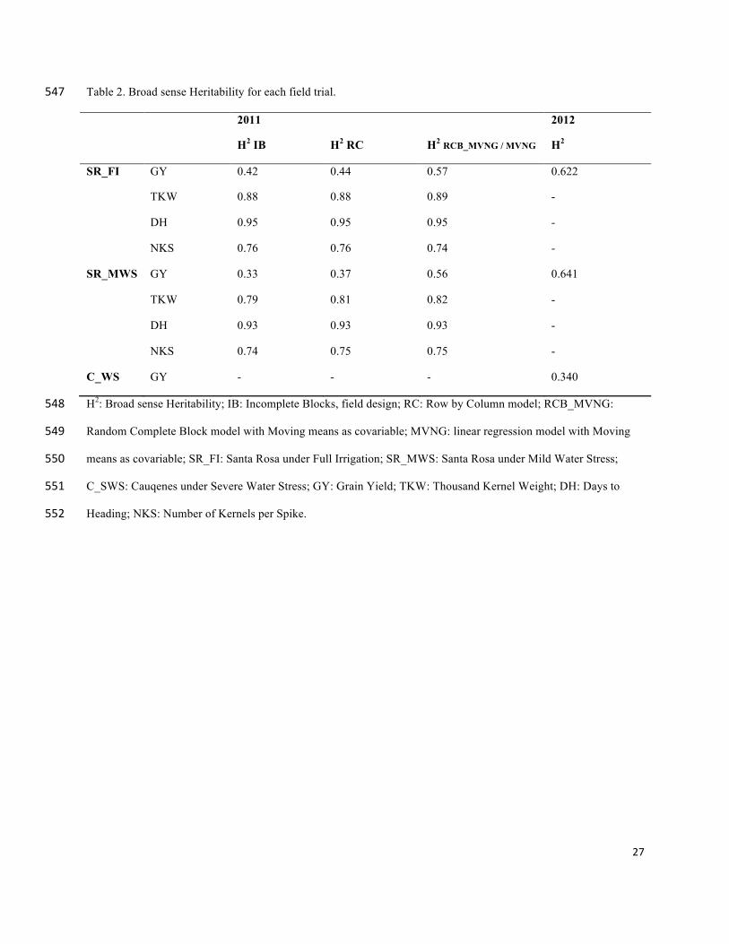
homogeneous residuals within the field (Figure 4 and Figure 5). In addition, the broad sense 266
heritability was calculated for each model. The highest heritability value was for the MVNG 267
model for all traits (Table 2). 268
In 2012 the fields had minimal spatial variation, therefore after adjusting the phenotypic data 269
with the intended field design, the residuals observed were homogeneous throughout the field. 270
The heritability for yield was higher for the 2012 trials than for the 2011 trials. Cauquenes, 271
which was a dryland condition with more drought stress, presented a more pronounced field 272
variation (Table 2) resulting in a lower heritability than the other two fields in 2012. 273
Phenotypic predictions: 274
A genomic selection model using the GBLUP approach was fitted for each trait, using the line 275
BLUPs of the best-fit phenotypic model. In all cases the 86% of genotypes were used to train the 276
14
genomic model and the predictions were assessed in the other 14 %. The predictions were 277
evaluated using 100 cross validations with the training and prediction sets randomly partitioned. 278
We determined the standard deviation across all correlation for each model. 279
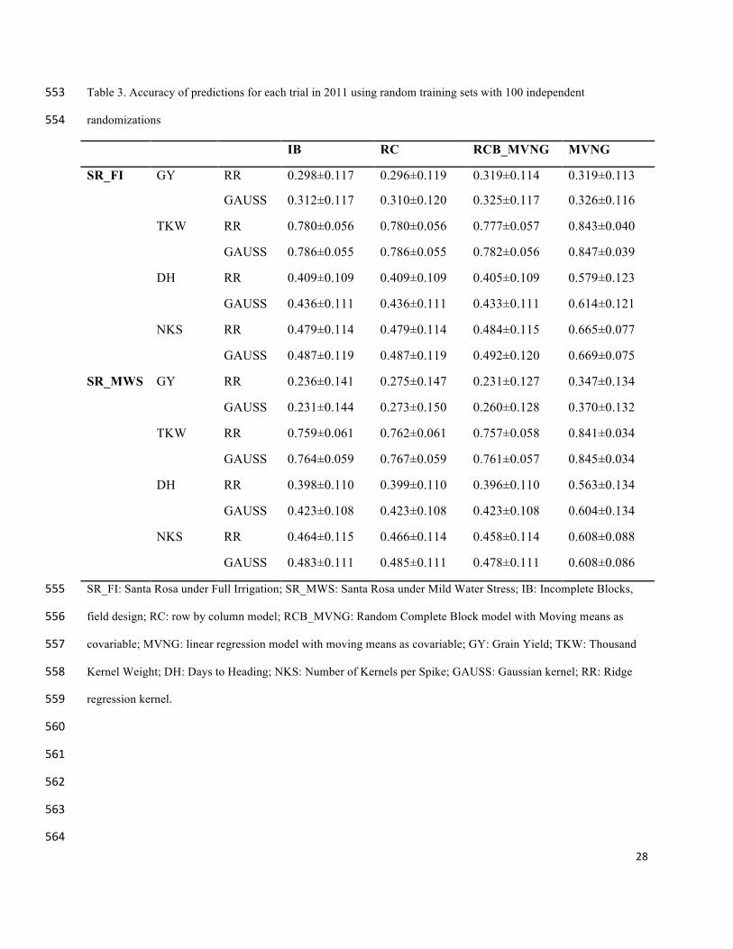
The RR and GAUSS kernels were tested for each GS model. In most of the cases GAUSS 280
performed better than RR. In general, the phenotypic data adjusted with MVNG, resulted in 281
higher prediction accuracies, although high standard errors were observed (Table 3). 282
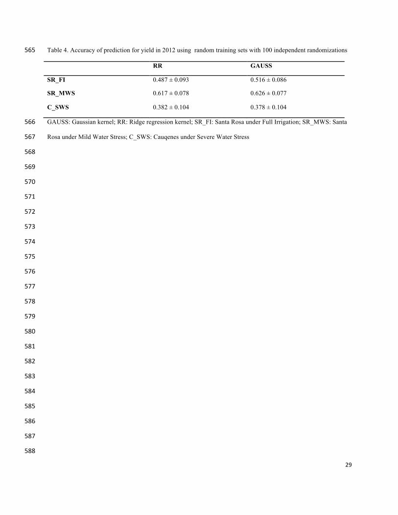
The prediction accuracies for 2012 were higher than for 2011 (Table 3 and Table 4). 283
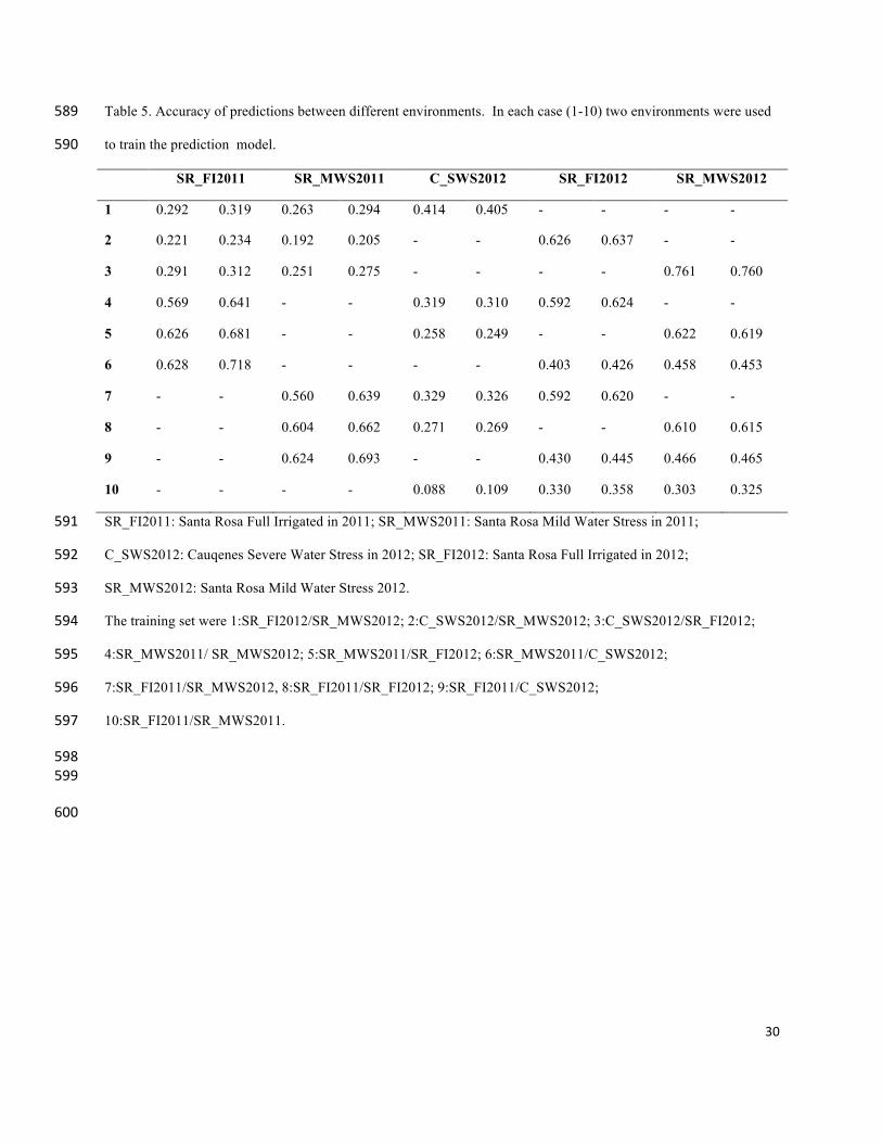
All possible combinations of the trials were used to test as training sets to observe the prediction 284
accuracy from year to year or from one environment to the next. Due to the high variation from 285
year to year, the best predictions were obtained when adding information in the model that 286
included both years (Table 5). 287
DISCUSSION 288
The challenge in wheat breeding is to accelerate the adaptation of germplasm for more efficient 289
and rapid results, increasing yield and adapting to less favorable future climates. Tools are now 290
available that allow taking up this challenge and relate the complex genetic mechanism involved 291
in phenotypic expression in relation with environmental interactions (Heffner et al. 2009). 292
Genotypic analysis: 293
Using GBS we identified and genotyped 102,324 SNPs across 384 breeding lines. This genetic 294
information was used to calculate a dissimilarity matrix, which was analyzed by PCoA . As 295
describe by Poland et al. (2012a) we did not observed differences between dissimilarity matrixes 296
calculates with and without imputation. For PCoA, the lines grouped by breeding program of 297
15
origin. This was expected as the lines from the same breeding program should be more similar 298
genetically because they share a common parental background and were bred under similar 299
developmental conditions (Rauf et al. 2010). 300
SNP tags from the breeding lines were anchored in the SynOpDH genetic map with 13% of the 301
tags aligning with high similarity. These tags were used to test LD between SNPs (Supplemental 302
data). As expected, high LD within groups were identified. In the same way, the distribution and 303
concentration of SNPs in different chromosomes was in agreement with other assessments of LD 304
in elite wheat breeding lines (Chao et al. 2010). We genetically anchored 13,357 SNPs, which 305
were well distributed across the genome. The calculated LD across individuals, confirmed high 306
correlations between closely linked SNPs on each linkage group (Supplement). 307
Phenotypic predictions: 308
Prior to making predictions the phenotypic data were adjusted and residuals in the model were 309
analyzed. The analysis showed a strong spatial effect across the field for the 2011 data. The 310
introduction of a spatial correction model accounted for some of this variation as observed by 311
higher heritability of measurements. A higher heritability indicates that a higher proportion of the 312
variance in the experiment is due to a difference between genotypes (Holland et al., 2003). The 313
mixed models for field effects that showed a higher heritability also showed an increase in the 314
mean accuracies of genomic predictions. The importance of taking into account appropriate field 315
design prior to the experiment has been demonstrated (Federer 2003; Federer and Crossa 2012). 316
If possible, variability in the field such as soil fertility, can be measured a prori and optimal field 317
designs applied. Analysis methods for a posteriori modeling of field variability have also been 318
described (Cullis et al. 1998; Piepho and Williams 2010). In this study we found these post data 319
16
adjustment to improve the quality of our data. As genotyping becomes less and less of a 320
constraint for developing genomic prediction training sets, proper treatment of phenotypic 321
observations is the key to increasing the accuracy of predictions. There are studies that include 322
sets of environmental variables in training models, which are measured during experiments, with 323
the objective to control these sources of variation and consider genotype x environmental 324
interactions (Chapman 2008). If the different sources of variation can be measured, together with 325
genotype x environment interactions, prediction accuracies should improve. 326
Another interest is the ability to predict phenotypes across environments, or from year to year 327
(Burgueño et al. 2012). However, when predicting new lines in previously untested 328
environments, most prediction power is lost. Therefore, it is important to generate a growing 329
database for model training, with corresponding sets of genotypes for the breeding program and 330
target environments and continually increase the number of environments tested. In the present 331
study, higher prediction accuracies were observed when using data from two years to train the 332
model (Table 5). When training the model with data from only one year, the accuracies of 333
predictions were low because the year-to-year correlation was low (Table 5). 334
The accuracies of predictions were comparable with other work in wheat, which have used 335
different fingerprinting approaches (Crossa et al. 2010; Heffner et al. 2011), adding confidence 336
to the GBS approach. 337
Two different statistical models were tested using the GBLUP approach. The highest prediction 338
accuracies were achieved with a Gaussian kernel. This model considers epistatic effects in 339
addition to additive effects modeled presented in RR models (Gianola and van Kaam 2008). 340
This study is part of a long term objective to adapt wheat germplasm to Mediterranean climate 341
environments of central Chile, and subsequently to other regions in South America. Previous 342
17
data (unpublished) suggests that the 384 lines present traits incorporated from the International 343
Maize and Wheat Improvement Center (CIMMYT), show adaptation to drier areas in Chile, and 344
both germplasm groups (INIA-Chile and INIA-Uruguay) have shown different degrees of 345
adaptation to these Chilean environments. We believe that this data set contains the necessary 346
genetic diversity for a germplasm base to start a breeding program guided towards drier areas in 347
Chile. 348
CONCLUSION 349
The development of new genotyping tools has been the framework to the practical 350
implementation of genomic selection. There are many crops with different genomic 351
characteristics that should be considered when identifying the most suited genotyping 352
methodology. In this study, GBS was successfully applied for the genome-wide characterization 353
of wheat breeding lines. GBS is a low-cost approach, which can be used to genotype thousands 354
of lines per year in a breeding program. 355
The challenge in leveraging genomic assisted breeding approaches in applied programs now 356
remains in obtaining high-quality and long-term accumulation of phenotypic data from multiple 357
years and targeted environments. This study showed an increase in prediction accuracy with 358
proper treatment of phenotypic data from field trials. High throughput and high precision 359
phenotyping tools are being tested and used, that will be well suited for breeding program and 360
increasing predictions. Understanding and predicting the complex interaction between genotype 361
and environment will also be key to select lines based on genotypic information. 362
363
Acknowledgements 364
18
This work was supported by the research grants FONTAGRO ATN/OC-11943 and FONDECYT 365
N° 1110732. We thank Alejandro Castro for technical assistance in field experiments. 366
367
368
REFERENCES 369
Akhunov, E. D., A. W. Goodyear, S. Geng, L.L. Qi, B. Echalier et al., 2003 The organization 370
and rate of evolution of wheat genomes are correlated with recombination rates along 371
chromosome arms. Gen. Res. 13: 753-763. 372
Altschul, S. F., W. Gish, W. Miller, E. W. Myers, and D. J. Lipman, 1990 Basic local alignment 373
search tool. J. Mol. Biol. 215: 403-410. 374
Bates, D., 2007 lme4: Linear mixed-effects models using s4 classes, pp. R package. 375
Bennett, M. D., and J. B. Smith, 1976 Nuclear DNA amounts in angiosperms. Philos. Trans. R 376
Soc. Lond. B Biol. Sci. 274: 227-274. 377
Buerstymayr, H., T. Ban, and J. A. Anderson, 2009 QTL mapping and marker-assisted selection 378
for Fusarium head blight resistance in wheat: a review. Plant Breeding 128: 1-26. 379
Burgueño, J., G. de los Campos, K. Weigel, and J. Crossa, 2012 Genomic Prediction of Breeding 380
Values when Modeling Genotype × Environment Interaction using Pedigree and Dense 381
Molecular Markers. Crop Science 52: 707-719. 382
Cabrera-Bosquet, L., J. Crossa, J. von Zitzewitz, M. D. Serret, and J. L. Araus, 2012 High-383
throughput phenotyping and genomic selection: the frontiers of crop breeding converge. 384
J. Integr. Plant Biol. 54: 312-320. 385
19
Chao, S., J. Dubcovsky, J. Dvorak, M. C. Luo, S. P. Baenziger et al., 2010 Population- and 386
genome-specific patterns of linkage disequilibrium and SNP variation in spring and 387
winter wheat (Triticum aestivum L.). BMC Genomics 11: 727-744. 388
Chapman, S. C., 2008 Use of crop models to understand genotype by environment interactions 389
for drought in real-world and simulated plant breeding trials. Euphytica 161: 195-208. 390
Collard, B. C. Y., M. Z. Z. Jahufer, J. B. Brouwer, and E. C. K. Pang, 2005 An introduction to 391
markers, quantitative trait loci (QTL) mapping and marker-assisted selection for crop 392
improvement: The basic concepts. Euphytica 142: 169–196. 393
Collard, B. C., and D. J. Mackill, 2008 Marker-assisted selection: an approach for precision plant 394
breeding in the twenty-first century. Philos. Trans. R Soc. Lond B Biol. Sci. 363: 557-395
572. 396
Crossa, J., J. Burgueño, P. L. Cornelius, G. McLaren, R. Trethowan et al., 2006 Modeling 397
Genotype × Environment Interaction Using Additive Genetic Covariances of Relatives 398
for Predicting Breeding Values of Wheat Genotypes. Crop Science 46: 1722–1733. 399
Crossa, J., G. de los Campos, P. Perez, D. Gianola, J. Burgueño et al., 2010 Prediction of genetic 400
values of quantitative traits in plant breeding using pedigree and molecular markers. 401
Genetics 186: 713-724. 402
Cullis, B., B. Gogel, A. Verbyla, R. Thompson, and A. Verbyla, 1998 Spatial Analysis of Multi-403
Environment Early Generation Variety Trials. Biometrics 54: 1-18. 404
de los Campos, G., D. Gianola, G. J. Rosa, K. A. Weigel, and J. Crossa, 2010 Semi-parametric 405
genomic-enabled prediction of genetic values using reproducing kernel Hilbert spaces 406
methods. Genet. Res. 92: 295-308. 407
20
del Pozo, A., and P. del Canto, 1999 Zonas agroclimáticas y sistemas productivos de la VII y VII 408
región. Instituto de Investigaciones Agropecuarias. Serie Quilamapu 113. 409
Dubcovsky, J., M. C. Luo, G. Y. Zhong, R. Bransteitter, A. Desai et al., 1996 Genetic map of 410
diploid wheat, Triticum monococcum L., and its comparison with maps of Hordeum 411
vulgare L.. Genetics 143: 983-999. 412
Dvorak, J., and H. B. Zhang, 1990 Variation in repeated nucleotide sequences sheds light on the 413
phylogeny of the wheat B and G genomes. Proc Natl Acad Sci U S A 87: 9640-9644. 414
Dvorak, J., P. Terlizzi, H. B. Zhang, and P. Resta, 1993 The evolution of polyploid wheats: 415
identification of the A genome donor species. Genome 36: 21-31. 416
Elshire, R. J., J. C. Glaubitz, Q. Sun, J. A. Poland, K. Kawamoto et al., 2011 A robust, simple 417
genotyping-by-sequencing (GBS) approach for high diversity species. PLoS One 6: 418
e19379. 419
Endelman, J. B., 2011 Ridge Regression and Other Kernels for Genomic Selection with R 420
Package rrBLUP. The Plant Genome Journal 4: 250-255. 421
FAOSTAT, 2011. http://faostat.fao.org/site/339/default.aspx 422
Federer, W. T., 2003 Exploratory Model Selection for Spatially Designed Experiments – Some 423
Examples. J. of Data Sci. 1:231–248. 424
Federer, W. T., and J., Crossa, 2012 I.4 Screening Experimental Designs for Quantitative Trait 425
Loci, Association Mapping, Genotype-by Environment Interaction, and Other 426
Investigations. Frontiers in physiology 3:1-8. 427
Gianola, D., M. Perez-Enciso, and M. A. Toro, 2003 On marker-assisted prediction of genetic 428
value: beyond the ridge. Genetics 163: 347–365. 429
21
Gianola, D., and J. B. van Kaam, 2008 Reproducing kernel hilbert spaces regression methods for 430
genomic assisted prediction of quantitative traits. Genetics 178: 2289-2303. 431
Gianola, D., H. Okut, K. A. Weigel, and G. J. Rosa, 2011 Predicting complex quantitative traits 432
with Bayesian neural networks: a case study with Jersey cows and wheat. BMC genetics 433
12: 87-101. 434
Goddard, M. E., B. J. Hayes, and T. H. E. Meuwissen, 2011 Using the genomic relationship 435
matrix to predict the accuracy of genomic selection. J. Anim. Breed. Genet. 128(6): 409–436
421. 437
Heffner, E. L., M. E. Sorrells, and J.-L. Jannink, 2009 Genomic Selection for Crop Improvement. 438
Crop Science 49: 1-12. 439
Heffner, E. L., J.-l. Jannink, and M. E. Sorrells, 2011 Genomic Selection Accuracy using 440
Multifamily Prediction Models in a Wheat Breeding Program. The Plant Genome Journal 441
4: 65-75. 442
Holland, J.B., W.E. Nyquist, and C.T. Cervantes-Martínez, 2003 Heritability for Plant Breeding: 443
An Update. Plant Breeding Reviews 22: 9–112. 444
Jansen, R., 1993. Interval mapping of multiple quantitative trait loci. Genetics 135: 205–211. 445
Kang, H. M., N. A. Zaitlen, C. M. Wade, A. Kirby, D. Heckerman et al., 2008 Efficient control 446
of population structure in model organism association mapping. Genetics 178: 1709-447
1723. 448
Kirigwi, F., M. Van Ginkel, G. Brown-Guedira, B. Gill, G. M. Paulsen et al., 2007 Markers 449
associated with a qtl for grain yield in wheat under drought. Molecular Breeding 20: 401-450
413. 451

22
Kraakman, A. T. W., R. E. Niks, P. M. M. M. Van den Berg, P. Stam, and F. A. Van Eeuwijk, 452
2004 Linkage disequilibrium mapping of yield and yield stability in modern spring barley 453
cultivars. Genetics 168: 435-446. 454
Lander, E. S., and D. Botstein, 1989 Mapping mendelian factors underlying quantitative traits 455
using RFLP linkage maps. Genetics 121: 185-199. 456
Landjeva, S., V. Korzun, and A. Börner, 2007 Molecular markers: actual and potential 457
contributions to wheat genome characterization and breeding. Euphytica 156: 271-296. 458
Le Gouis, J., J. Bordes, C. Ravel, E. Heumez, S. Faure et al., 2012 Genome-wide association 459
analysis to identify chromosomal regions determining components of earliness in wheat. 460
Theor. Appl. Genet. 124: 597-611. 461
Leiser, W. L., H. F. Rattunde, H.-P. Piepho, and H. K. Parzies, 2012 Getting the Most Out of 462
Sorghum Low-Input Field Trials in West Africa Using Spatial Adjustment. Journal of 463
Agronomy and Crop Science 198: 349-359. 464
Masuka, B., J. L. Araus, B. Das, K. Sonder, and J. E. Cairns, 2012 Phenotyping for abiotic stress 465
tolerance in maize. J. Integr. Plant Biol. 54: 238-249. 466
Meuwissen, T. H., B. J. Hayes, and M. E. Goddard, 2001 Prediction of Total Genetic Value 467
Using Genome-wide Dense Marker Maps. Genetics 157: 1819–1829. 468
Müller, B. U., A. Schützenmeister, and H.-P. Piepho, 2010 Arrangement of check plots in 469
augmented block designs when spatial analysis is used. Plant Breeding 129: 535-542. 470
Neumann, K., B. Kobiljski, S. Denčić, R. K. Varshney, and A. Börner, 2010 Genome-wide 471
association mapping: a case study in bread wheat (Triticum aestivum L.). Molecular 472
Breeding 27: 37-58. 473
23
Paradis, E., J. Claude, and K. Strimmer, 2004 APE: Analyses of Phylogenetics and Evolution in 474
R language. Bioinformatics 20: 289-290. 475
Peiris, T. U. S., S. Samita, and W. H. D. Veronica, 2008 Accounting for Spatial Variability in 476
Field Experiments on Tea. Experimental Agriculture 44: 547-557. 477
Piepho, H. P., and E.R., Williams, 2010 Linear variance models for plant breeding trials. Plant 478
Breeding 129:1–8. 479
Poland, J. A., P. J. Brown, M. E. Sorrells, and J. L. Jannink, 2012a Development of high-density 480
genetic maps for barley and wheat using a novel two-enzyme genotyping-by-sequencing 481
approach. PLoS One 7: e32253. 482
Poland, J., J. Endelman, J. Dawson, J. Rutkoski, S. Wu et al., 2012b Genomic Selection in 483
Wheat Breeding using Genotyping-by-Sequencing. The Plant Genome Journal 5: 1-11. 484
Poland, J. a., and T. W. Rife, 2012 Genotyping-by-Sequencing for Plant Breeding and Genetics. 485
The Plant Genome Journal 5: 547-557. 486
Pritchard, J. K., M. Stephens, N.A. Rosenberg, and P. Donnelly, 2000 Association mapping in 487
structured populations. Am. J. Hum. Genet. 67: 170–181. 488
Rauf, S., J. A. Teixeira, A. Ali, and K. Abdul, 2010 Consequences of Plant Breeding on Genetic 489
Diversity. International Journal Of Plant Breeding 4: 1-21. 490
R Core Team, 2013 R: A Language and Environment for Statistical Computing. R Foundation 491
for Statistical Computing, Vienna, Austria. http://www.R-project.org 492
Risch N., and K. Merikangas, 1996 The future of genetic studies of complex human diseases. 493
Science 273:1516–1517. 494
Sarkar, P., and G. L. Stebbins, 1956 Morphological evidence concerning the B genome in wheat. 495
American Journal of Botany 43: 1-8. 496
24
Schwender, H., Q. Li, C. Neumann, and I. Ruczinski, 2012 trio: trio package whithout Fortran 497
code, pp. R package. 498
Shin, J. H., S. Blay, B. McNeney, and J. Graham, 2006 LDheatmap: An R Function for 499
Graphical Display of Pairwise Linkage Disequilibrium Between Single Nucleotide 500
Polymorphisms. Journal of Statistical Software 16: 1-9. 501
Sonah, H., M. Bastien, E. Iquira, A. Tardivel, G. Legare et al., 2013 An improved genotyping by 502
sequencing (GBS) approach offering increased versatility and efficiency of SNP 503
discovery and genotyping. PLoS One 8: e54603. 504
Tanksley, S. D., 1993 Mapping Polygenes. Annu. Rev. Genet. 27: 205–233. 505
Technow, F., 2012 Software for moving grid adjustment in plant breeding field trials, pp. R 506
Package for moving grid adjustment in plant breeding field trials. 507
White, J. W., P. Andrade-Sanchez, M. A. Gore, K. F. Bronson, T.A. Coffelt et al., 2012 Field-508
based phenomics for plant genetics research. Field Crops Research 133: 101-112. 509
Xu, S., 2003 Theoretical basis of the Beavis effect. Genetics 165: 2259-2268. 510
Yu, L. X., A. Morgounov, R. Wanyera, M. Keser, S. K. Singh et al., 2012 Identification of Ug99 511
stem rust resistance loci in winter wheat germplasm using genome-wide association 512
analysis. Theor. Appl. Genet. 125: 749-758. 513
514
515
516
517
518
519
25
Figure 1. Diagram to calculate the covariable xi. Yi is the phenotypic value in the plot. The neighboring plots are 520
indicated with grey color. 521
Figure 2. Principal Coordinate Analysis from dissimilarity matrix calculated with genetic data. Points in red 522 represent advanced lines from the INIA Chile breeding program, green points identified lines from CIMMYT and 523
blue points denote advanced lines and pre-breeding lines from the INIA Uruguay breeding program. 524
Figure 3. GBS based SNP distribution on each wheat chromosomes. 525
Figure 4. Plot residuals along the field for each model analysis for Santa Rosa Irrigated. The color scale shows the 526 value of residuals as indicated. A) Residuals for IB; B) Residuals for RC; C) Residuals for RCB_MVNG; D) 527
Residuals for MVNG. 528
Figure 5. Plot residuals along the field for each model analysis for Santa Rosa Non-Irrigated trial. The color scale 529 shows the value of residual effects as indicated. A) Residuals for IB; B) Residuals for RC; C) Residuals for 530
RCB_MVNG; D) Residuals for MVNG 531
532
533
26
Table 1. Description of models used to adjust the phenotypic data 534
Model Name Model Expression
IB y = g i + repj + bl(rep)ijk + eijk
RC y = g i +rep j + fil(rep) jk + col(rep) jl + eijkl
RCB_MVNG y = gi + βxj + repk + eijk
MVNG y = u + βxi + ei
g: treatment, u: general mean , rep: repetitions, bl(rep): incompletes blocks nested in repetitions, fil(rep): rows 535
nested in repetitions, col(rep): columns nested in repetitions, e: residual, x: covariable as phenotypic value of plot 536
minus means of neighbors plots within grid. IB: incomplete blocks, field design; RC: row by column model; 537
RCB_MVNG: random complete block model with moving means as covariable; MVNG: linear regression model 538
with moving means as covariable. 539
540
541
542
543
544
545
546
27
Table 2. Broad sense Heritability for each field trial. 547
2011 2012
H2 IB H2 RC H2 RCB_MVNG / MVNG H2
SR_FI GY 0.42 0.44 0.57 0.622
TKW 0.88 0.88 0.89 -
DH 0.95 0.95 0.95 -
NKS 0.76 0.76 0.74 -
SR_MWS GY 0.33 0.37 0.56 0.641
TKW 0.79 0.81 0.82 -
DH 0.93 0.93 0.93 -
NKS 0.74 0.75 0.75 -
C_WS GY - - - 0.340
H2: Broad sense Heritability; IB: Incomplete Blocks, field design; RC: Row by Column model; RCB_MVNG: 548
Random Complete Block model with Moving means as covariable; MVNG: linear regression model with Moving 549
means as covariable; SR_FI: Santa Rosa under Full Irrigation; SR_MWS: Santa Rosa under Mild Water Stress; 550
C_SWS: Cauqenes under Severe Water Stress; GY: Grain Yield; TKW: Thousand Kernel Weight; DH: Days to 551
Heading; NKS: Number of Kernels per Spike. 552
28
Table 3. Accuracy of predictions for each trial in 2011 using random training sets with 100 independent 553
randomizations 554
IB RC RCB_MVNG MVNG
SR_FI GY RR 0.298±0.117 0.296±0.119 0.319±0.114 0.319±0.113
GAUSS 0.312±0.117 0.310±0.120 0.325±0.117 0.326±0.116
TKW RR 0.780±0.056 0.780±0.056 0.777±0.057 0.843±0.040
GAUSS 0.786±0.055 0.786±0.055 0.782±0.056 0.847±0.039
DH RR 0.409±0.109 0.409±0.109 0.405±0.109 0.579±0.123
GAUSS 0.436±0.111 0.436±0.111 0.433±0.111 0.614±0.121
NKS RR 0.479±0.114 0.479±0.114 0.484±0.115 0.665±0.077
GAUSS 0.487±0.119 0.487±0.119 0.492±0.120 0.669±0.075
SR_MWS GY RR 0.236±0.141 0.275±0.147 0.231±0.127 0.347±0.134
GAUSS 0.231±0.144 0.273±0.150 0.260±0.128 0.370±0.132
TKW RR 0.759±0.061 0.762±0.061 0.757±0.058 0.841±0.034
GAUSS 0.764±0.059 0.767±0.059 0.761±0.057 0.845±0.034
DH RR 0.398±0.110 0.399±0.110 0.396±0.110 0.563±0.134
GAUSS 0.423±0.108 0.423±0.108 0.423±0.108 0.604±0.134
NKS RR 0.464±0.115 0.466±0.114 0.458±0.114 0.608±0.088
GAUSS 0.483±0.111 0.485±0.111 0.478±0.111 0.608±0.086
SR_FI: Santa Rosa under Full Irrigation; SR_MWS: Santa Rosa under Mild Water Stress; IB: Incomplete Blocks, 555
field design; RC: row by column model; RCB_MVNG: Random Complete Block model with Moving means as 556
covariable; MVNG: linear regression model with moving means as covariable; GY: Grain Yield; TKW: Thousand 557
Kernel Weight; DH: Days to Heading; NKS: Number of Kernels per Spike; GAUSS: Gaussian kernel; RR: Ridge 558
regression kernel. 559
560
561
562
563
564
29
Table 4. Accuracy of prediction for yield in 2012 using random training sets with 100 independent randomizations 565
RR GAUSS
SR_FI 0.487 ± 0.093 0.516 ± 0.086
SR_MWS 0.617 ± 0.078 0.626 ± 0.077
C_SWS 0.382 ± 0.104 0.378 ± 0.104
GAUSS: Gaussian kernel; RR: Ridge regression kernel; SR_FI: Santa Rosa under Full Irrigation; SR_MWS: Santa 566
Rosa under Mild Water Stress; C_SWS: Cauqenes under Severe Water Stress 567
568
569
570
571
572
573
574
575
576
577
578
579
580
581
582
583
584
585
586
587
588
30
Table 5. Accuracy of predictions between different environments. In each case (1-10) two environments were used 589
to train the prediction model. 590
SR_FI2011 SR_MWS2011 C_SWS2012 SR_FI2012 SR_MWS2012
1 0.292 0.319 0.263 0.294 0.414 0.405 - - - -
2 0.221 0.234 0.192 0.205 - - 0.626 0.637 - -
3 0.291 0.312 0.251 0.275 - - - - 0.761 0.760
4 0.569 0.641 - - 0.319 0.310 0.592 0.624 - -
5 0.626 0.681 - - 0.258 0.249 - - 0.622 0.619
6 0.628 0.718 - - - - 0.403 0.426 0.458 0.453
7 - - 0.560 0.639 0.329 0.326 0.592 0.620 - -
8 - - 0.604 0.662 0.271 0.269 - - 0.610 0.615
9 - - 0.624 0.693 - - 0.430 0.445 0.466 0.465
10 - - - - 0.088 0.109 0.330 0.358 0.303 0.325
SR_FI2011: Santa Rosa Full Irrigated in 2011; SR_MWS2011: Santa Rosa Mild Water Stress in 2011; 591
C_SWS2012: Cauqenes Severe Water Stress in 2012; SR_FI2012: Santa Rosa Full Irrigated in 2012; 592
SR_MWS2012: Santa Rosa Mild Water Stress 2012. 593
The training set were 1:SR_FI2012/SR_MWS2012; 2:C_SWS2012/SR_MWS2012; 3:C_SWS2012/SR_FI2012; 594
4:SR_MWS2011/ SR_MWS2012; 5:SR_MWS2011/SR_FI2012; 6:SR_MWS2011/C_SWS2012; 595
7:SR_FI2011/SR_MWS2012, 8:SR_FI2011/SR_FI2012; 9:SR_FI2011/C_SWS2012; 596
10:SR_FI2011/SR_MWS2011. 597
598 599
600