increase in the carbon dioxide infrared emissions during solar proton events
TRANSCRIPT
151
ISSN 0016-7932, Geomagnetism and Aeronomy, 2006, Vol. 46, No. 2, pp. 151–158. © Pleiades Publishing, Inc., 2006.Original Russian Text © V.P. Ogibalov, S.N. Khvorostovskii, G.M. Shved, 2006, published in Geomagnetizm i Aeronomiya, 2006, Vol. 46, No. 2, pp. 159–167.
1. INTRODUCTION
As a result of a decrease in the molecular collisionfrequency with altitude, not only collisional vibrationaltransitions but also optical transitions contribute to theformation of the
CO
2
vibrational state population in themesosphere and lower thermosphere (MLT) [López-Puertas and Taylor, 2001]. Therefore, the population ofthese states in the MLT region becomes non-Boltz-mann; i.e., the local thermodynamic equilibrium (LTE)is disturbed for vibrational states. The disturbance ofLTE for the states excited due to the deformation vibra-tion (
ν
2
) of
CO
2
molecule begins from approximately70 km [Khvorostovskaya et al., 2002]. The same distur-bance but for the states excited due to the stretchingasymmetrical vibration (
ν
3
) begins from approximately60 km at night and even from lower altitudes (fromapproximately 50 km) in daytime due to the excitationof vibrational states during solar radiation absorption in
CO
2
infrared bands [Shved et al., 1998].
Optical transitions, when the vibrational quantumnumber corresponding to the
ν
2
vibration changes byunity, generate atmospheric emission in the 15
µ
m
CO
2
band. The same transitions but for the
ν
3
vibration pro-duce emission in the 4.3
µ
m band. Nonequilibrium(nonthermal) MLT emissions in the above bands werefirst measured in 1973–1974 on rockets that registeredemission from the zenith [Stair et al., 1974, 1975]. Sub-sequently, the nighttime and daytime nonequilibriumMLT emissions in these and other infrared vibrational–rotational
CO
2
bands were intensely studied duringboth rocket-borne and satellite observations and using
numerical simulation [
L
ó
pez
-Puertas and Taylor,2001]. Some researchers even tried to measure the 4.3and 15
µ
m emissions in order to determine the
CO
2
mixture ratio in the MLT region [Kaufmann et al.,2002; Mertens et al., 2003; Kostsov and Timofeev,2003].
Nighttime rocket-borne measurements of the4.3
µ
m emission at a latitude of
65°
N [Stair et al.,1975] indicated that the brightness of this emission inthe MLT region increases by an order of magnitude andmore during auroras. Some researchers tried to simu-late this enhancement [Kumer, 1977, 1978]. Theenhancement is explained by excitation of nitrogenvibrational states when
N
2
molecules are bombarded byenergetic electrons precipitating during auroras andvibrational excitation is subsequently transferred to
CO
2
molecules in the course of
N
2
–CO
2
collisions. Thisprocess of vibrational energy exchange is very rapidbecause the vibrational quantum energy (
ν
3
) is close tothe energy of vibrational quantum of
N
2
molecule. Inthe 1990s, some researchers became interested insprites, i.e., optical emission bursts in the mesospherethat occur above thunderclouds simultaneously withlightning strokes [Pasko et al., 1997]. Lightning strokesare accompanied by the generation of strong short-lived(~10 ms) quasielectrostatic fields at altitudes of 50–95 km. Atmospheric electrons are accelerated in thesefields and excite states of air molecules. As in the caseof auroras, excitation of
N
2
(1)
states should result in anenhancement of emission in the 4.3
µ
m
CO
2
band in theMLT region. The models of this enhancement were,
Increase in the Carbon Dioxide Infrared Emissions during Solar Proton Events
V. P. Ogibalov, S. N. Khvorostovskii, and G. M. Shved
V. A. Fok Research Institute of Physics, St. Petersburg State University, St. Petersburg, Russia
e-mail: [email protected]
Received November 10, 2004
Abstract
—Increase in the nighttime high-latitude nonthermal emissions in the mesosphere and lower thermo-sphere in the 4.3 and 15
µ
m
CO
2
bands during solar proton events has been estimated for the first time. Theestimations have been performed for protons with energies not lower than 1 MeV precipitating into the atmo-sphere. A strong increase in the 4.3
µ
m emission can be anticipated during the above events; however, a sub-stantial increase in the 15
µ
m emission is improbable. The 4.3
µ
m emission can increase only above approxi-mately 80 km regardless of the energy of precipitating protons. The excitation of CO
2
vibrational states, tran-sitions from which generate the 4.3
µ
m emission, is caused by the vibrational excitation of
N
2
molecules dueto collisions with secondary electrons, produced during solar proton events, and the following transfer of thisexcitation to
CO
2
(00
0
1)
molecules during
N
2
–CO
2
collisions.
PACS numbers: N94.20D
DOI:
10.1134/S0016793206020034
152
GEOMAGNETISM AND AERONOMY
Vol. 46
No. 2
2006
OGIBALOV et al.
correspondingly, proposed [Picard et al., 1997; Milikhet al., 1998].
In addition to the above causes, energetic electronsare also originated in the MLT region during solar pro-ton events (SPEs) (see, e.g., [Bazilevskaya et al.,2003]). In the present study the
CO
2
vibrational statepopulations, excited as a result of high-energy electronprecipitation into the atmosphere during these events,are calculated for the first time. The populations are cal-culated for nighttime conditions; i.e., in the case whenthe states are not excited during solar radiation absorp-tion. The obtained populations are used to simulate ver-tical profiles of emission intensities in the 4.3 and15
µ
m
CO
2
bands for two versions of emission registra-tion: from the zenith and planetary limb. The estima-tions are performed for the proton energy distributionsregistered during SPEs of July 16, 1959, August 4,1972, and July 13, 1982, and presented in [Solomonet al., 1983].
2. MODEL DESCRIPTIONThe vertical profile of the atmospheric temperature,
typical of the high-latitude MLT region in the secondhalf of the summer, was selected based on the MSISE-90 model of the atmosphere [Hedin, 1991]. The modelof the composition of the atmosphere was taken from[Shved et al., 1998].
The vibrational state systems and optical and colli-sional vibrational transitions used in the calculationswere described in detail by Shved et al. [1998]. Thesame work presents the rate constants of the collisionalprocesses except for the rate constant of the
CO
2
(01
1
0)
state quenching during
CO
2
–O
collisions, which wastaken from [Khvorostovskaya et al., 2002]. The intensi-ties of the
CO
2
vibrational–rotational lines are takenfrom the HITRAN-2000 database for the spectroscopicparameters of atmospheric molecules. The appliedmodel of the Lorentz width of these lines is presentedin [Shved et al., 1998]. Additional excitation of
CO
2
vibrational states in the vicinity of the mesopause dueto the transfer of the vibrational excitation energy ofOH molecule to these states [Shved et al., 1998] wasignored in these estimates of the molecule state popula-tion since the rate of this excitation is very uncertain.
The energy of energetic protons precipitating duringSPEs dissipates in the atmosphere and is transformed incascade into the energy of the secondary particles—hydrogen atoms, protons, and electrons—during colli-sions [Eather, 1967]. Produced energetic electronsshow a specific energy distribution [Khvorostovskiiand Zelenkova, 1997b; Khvorostovskii, 2001a], andcollisions with these electrons represent the mainmechanism of additional excitation of air moleculevibrational states during SPEs. We took into accountdifferent ways that result in excitation of
ν
2
and
ν
3
vibrations of
CO
2
molecule. First of all, we took intoaccount direct excitation of the
01
1
0, 2
ν
2
, and
00
0
1
states during collision of
CO
2
(00
0
0)
molecule withelectron, where
2
ν
2
denotes the set of the
10
0
0, 02
2
0
,and
02
0
0
states that have close energies and are interre-lated via rapid intramolecular vibrational energyexchange during collisions [Shved et al., 1998;Ogibalov et al., 1998]. As in the case when the 4.3
µ
memission was generated during auroras and lightningstrokes (see Introduction), we took into account themost effective mechanism of the
CO
2
(00
0
1)
state exci-tation by electrons, which represents the sequence ofthe processes
N
2
(0) +
e
N
2
(
v
) +
e,
(1)
CO
2
(00
0
0) + N
2
(1) CO
2
(00
0
1) + N
2
(0). (2)
In so doing, we assumed that
N
2
(
v
)
molecules with thevibrational quantum number
v
> 1 almost instanta-neously redistribute their excitation over
N
2
(1)
mole-cules since the rate of the vibrational energy exchangebetween nitrogen molecules during their collision ishigh. We also took into account additional pumping ofthe nitrogen molecule vibrational states as a result ofthe sequence of the processes
O(
3
P) +
e
O(1D) + e, (3)
N2(0) + O(1D) N2(v) + O(3P). (4)
In this case the rate of the process (4) was taken from[Shved et al., 1998]. Finally, for the generation of the 15µm emission, we took into account pumping of themolecular oxygen vibrational states by electrons with asubsequent vibrational energy exchange during O2–CO2 collisions:
O2(0) + e O2(v) + e, (5)
CO2(0000) + O2(1) CO2(2ν2) + O2(0). (6)
As in the situation with N2(v) molecules, we alsoassumed that the entire vibrational excitation of oxygenmolecules is almost instantaneously concentrated inO2(1) molecules.
Excitation cross sections of the considered statesduring collisions with electrons were taken from [Chen,1964; Engelhardt et al., 1964] for N2(v), from [Linderand Schmidt, 1971] for O2(v), from [Bulos and Phelps,1976; Kochetov et al., 1979] for CO2(0110, 2ν2, 0001),and from [Thomas et al., 1997] for O(1D). The excita-tion rates of the above states by electrons were esti-mated using the method presented in Appendix forthree SPEs, the proton energy spectra for which aregiven in [Solomon et al., 1983]. In that paper thesespectra are presented for protons with an energy of Ep >1 MeV. Since a depth of primary proton penetrationinto the atmosphere decreases with decreasing Ep,ignored protons with Ep < 1 MeV almost do not pene-trate into the atmosphere below 90 km altitude[Khvorostovskii, 2001b]. However, these protons causeadditional pumping of molecular states above this alti-tude during SPEs. Therefore, the populations of the
GEOMAGNETISM AND AERONOMY Vol. 46 No. 2 2006
INCREASE IN THE CARBON DIOXIDE INFRARED EMISSIONS 153
excited molecule states above 90 km evaluated by usand the emission intensities determined based on thesevalues should be considered as lower estimates.
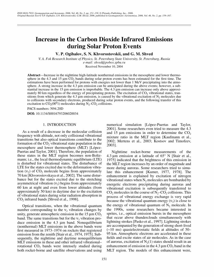
The vertical profiles of the rate of pumping the nitro-gen vibrational quanta in the processes (1) calculatedfor one N2 molecule are shown in Fig. 1. The pumpingrates of O22(1), CO2(0110), CO2(2ν2), CO2(0001), andO(1D) states calculated for one molecule of the consid-ered gas are equal to the pumping rate in Fig. 1 multi-plied by 14, 60, 14, 33, and 1.2 × 10⁻², respectively. Thesingularities of the proton energy spectra are responsi-ble for the specific features of the state pumping rateprofile. Primary protons with Ep < 3 MeV do not pene-trate below approximately 80 km. Therefore, during theseries of SPEs of July 16, 1959–August 4, 1972– July13, 1982, the pumping rate above this altitude increasedas a result of the corresponding increase in the spectraldensity of the flux of protons with the above energy.
The method for calculating population vibrationalstates is presented in [Kutepov et al., 1998].
3. RESULTS AND DISCUSSION
Population of molecular states
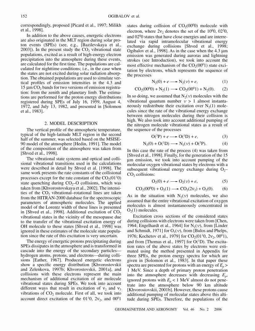
The population of the 12C16O2(0001), N2(1), andO2(1) excited vibrational states for the considered SPEsis shown in Fig. 2. The population of the ith state is tra-ditionally presented in terms of vibrational temperatureTv:
(7)
where k is the Boltzmann constant; Ei and gi are theenergy and degeneracy of the ith state, respectively; andni is the molecule concentration in this state. The sub-script 0 corresponds to the ground vibrational state. Themain specific features of the vertical variations Tv forthe molecule states presented in Fig. 2 and for otherCO2 vibrational states considered in the problem wererepeatedly discussed previously (see, e.g., [Shved et al.,1998; Ogibalov et al., 1998; López-Puertas and Taylor,2001]). In the atmosphere disturbed by precipitatingprotons, these features are as follows successively forthe CO2(0001), N2(1), and O2(1) states.
(i) In the layer of disturbed LTE, Tv(0001) relativelyweakly (as compared to a change in the atmospherictemperature, T) varies with altitude for both 12C16O2molecule and rare CO2 isotopes. This weak variabilityof Tv(0001) is related to the fact that the population ofthe CO2(0001) state is controlled by the optical pump-ing of the state by the atmospheric radiation comingfrom below.
(ii) To a certain altitude in the MLT region,Tv[N2(1)] is close to Tv(0001) owing to a rapid vibra-tional quantum energy exchange during N2–CO2 colli-
Tv i( )Ei
k gin0/g0ni( )ln-----------------------------------,=
sions. Since the atmosphere is rarefied, the rate of thisexchange decreases with increasing altitude, and otherprocesses begin to predominate in the population of theN2(1) state. At a sufficiently high thermospheric alti-tude, Tv[N2(1)] tends to T since the O mixing ratioincreases with increasing altitude and, correspondingly,the exchange rate of the vibrational and translationalenergy during N2–O collisions strongly increase.
(iii) The specific features of the vertical variations inTv[N2(1)] are explained similarly to the features of suchvariations in Tv[O2(1)]. The only difference consists inthat LTE takes place for the O2(1) state to a certain alti-tude in the MLT region.
Figure 2 indicates that the effect of SPEs on the mol-ecule state populations becomes appreciable onlyabove 75 km altitude, which is reached by protons withEp ~ 5 MeV. The O2(1) state population is especiallydisturbed by precipitating protons: Tv[O2(1)] canincrease by 100 K and even more. However, the process(6) is not so rapid that it could lead to a considerableincrease in Tv for the CO2(2ν2) states and related opticaland collisional transitions of the CO2(0110) state. For
1Ö–11
70
Altitude, km
80
90
100
110
120
Production rate, s–11Ö–10 1Ö–9 1Ö–8 1Ö–7 1Ö–61Ö–12
Fig. 1. Production rate of nitrogen vibrational quanta, cal-culated for one N2 molecule, due to collisions of N2 mole-cules with secondary electrons originated in the atmosphereduring SPEs of July 16, 1959 (solid line), August 4, 1972(dashes), and July 13, 1982 (dot-and-dash line) for the ver-tical precipitation of primary protons into the atmosphere.Curves indicate the total production rate of N2(1) mole-cules, which takes into account the excitation of N2(0) mol-ecules by electron impact to any vibrational state v with asubsequent transfer of the N2(v) molecule energy into thenumber (v) of N2(1) molecules owing to a rapid exchangeof vibrational quantum energy of nitrogen molecules duringtheir collisions.
154
GEOMAGNETISM AND AERONOMY Vol. 46 No. 2 2006
OGIBALOV et al.
150
70
80
90
100
110
120
200 250 300T, K
150 200 250 300 150 200 250 300T, K T, K
z, kmJuly 16, 1959 August 4, 1972 July 13, 1982
60
Fig. 2. Nighttime vibrational temperatures of the 12C16O2(0001) (solid lines), N2(1) (dashes), and O22(1) (dot-and-dash lines) statescorresponding to three SPEs (thick lines) as compared to the vibrational temperatures of the above states in the atmosphere, undis-turbed by precipitating protons (thin lines), as a function of altitude (z). Dotted line correspond to the model kinetic temperature ofthe atmosphere.
example, for the strongest of the considered populationdisturbances produced by SPE of July 13, 1982, Tv forthe 1000 and 0110 states of 12C16O2 molecule maximallyincrease in the layer 90–95 km by 1.4 and 0.1 K,respectively. Such an increase in Tv does not lead to anincrease in the concentration of CO2 molecules in theconsidered states by more than 10 and 0.3%, respec-tively.
As a result of an additional excitation of the N2(1)state during SPE, the dependence of the population ofthis state on that of the CO2(0001) state via the process(2) decreases: the Tv[N2(1)] and Tv(0001) profilesdiverge at lower altitudes than in the undisturbed atmo-sphere by approximately 10 km. During SPE, Tv[N2(1)]can increase in the lower thermosphere by about 100 K.
As in the case of auroras and sprites (see Introduc-tion), the processes (1) and (2) absolutely predominateduring SPE in pumping the CO2(0001) state. The contri-bution of the remaining considered processes of addi-tional excitation of this state is negligible. The Tv(0001)temperature can increase during proton precipitation by20–30 K, which corresponds to an increase in the con-centration of CO2(0001) molecules by several fold. Tak-ing into account that we underestimated additionalpumping the states above 90 km, the concentration of
these molecules in the lower thermosphere can behigher by an order of magnitude and more.
Emission Intensity
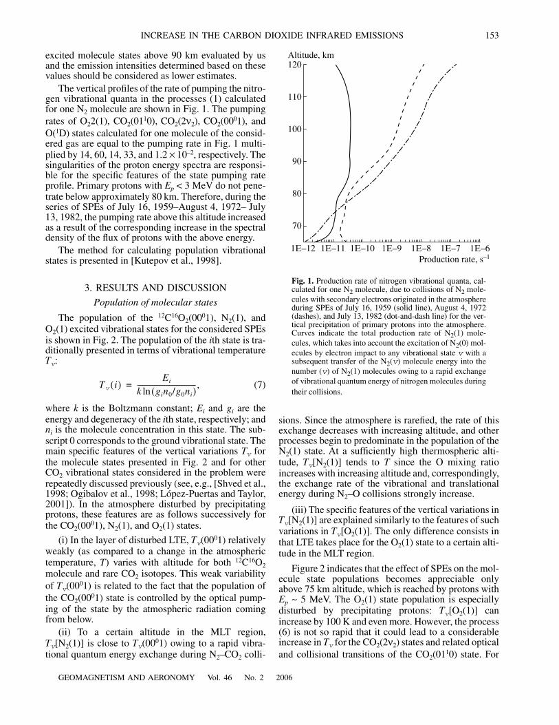
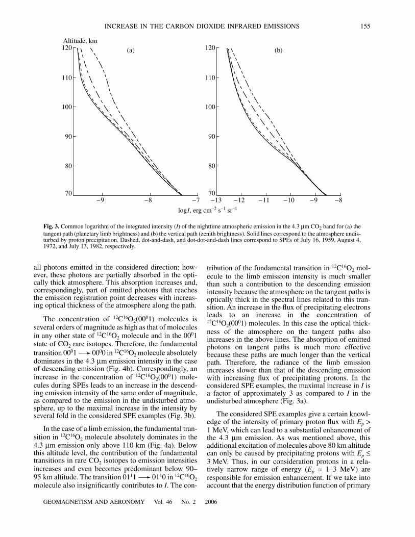
Figure 3 presents the vertical profiles of the inte-grated intensity (I) of emission in the 4.3 µm CO2 bandbased on the populations of the CO2 molecule vibra-tional states calculated for the considered SPEs. Forany geometry of observations, emission intensity canperceptibly increase during SPEs only above 80 km.This conclusion remains also valid in the case when wecan take into account excitation of air molecules byprotons precipitating with Ep < 1 MeV and spendingtheir energy above 90 km altitude.
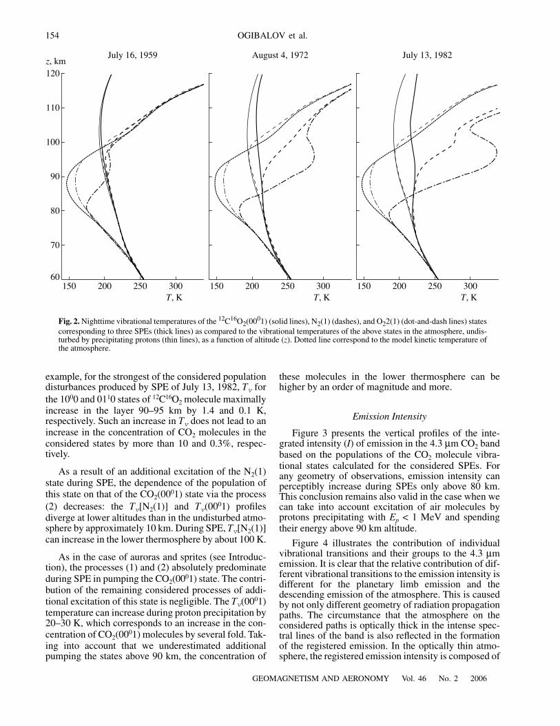
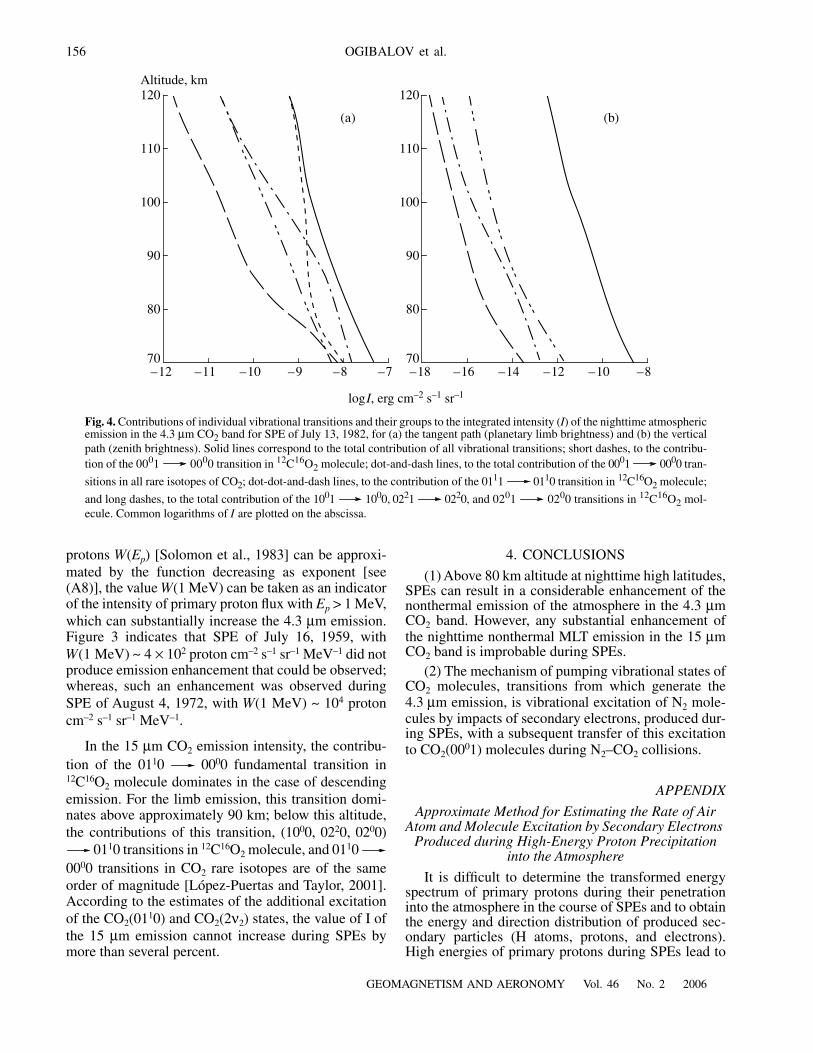
Figure 4 illustrates the contribution of individualvibrational transitions and their groups to the 4.3 µmemission. It is clear that the relative contribution of dif-ferent vibrational transitions to the emission intensity isdifferent for the planetary limb emission and thedescending emission of the atmosphere. This is causedby not only different geometry of radiation propagationpaths. The circumstance that the atmosphere on theconsidered paths is optically thick in the intense spec-tral lines of the band is also reflected in the formationof the registered emission. In the optically thin atmo-sphere, the registered emission intensity is composed of
GEOMAGNETISM AND AERONOMY Vol. 46 No. 2 2006
INCREASE IN THE CARBON DIOXIDE INFRARED EMISSIONS 155
all photons emitted in the considered direction; how-ever, these photons are partially absorbed in the opti-cally thick atmosphere. This absorption increases and,correspondingly, part of emitted photons that reachesthe emission registration point decreases with increas-ing optical thickness of the atmosphere along the path.
The concentration of 12C16O2(0001) molecules isseveral orders of magnitude as high as that of moleculesin any other state of 12C16O2 molecule and in the 0001state of CO2 rare isotopes. Therefore, the fundamentaltransition 0001 0000 in 12C16O2 molecule absolutelydominates in the 4.3 µm emission intensity in the caseof descending emission (Fig. 4b). Correspondingly, anincrease in the concentration of 12C16O2(0001) mole-cules during SPEs leads to an increase in the descend-ing emission intensity of the same order of magnitude,as compared to the emission in the undisturbed atmo-sphere, up to the maximal increase in the intensity byseveral fold in the considered SPE examples (Fig. 3b).
In the case of a limb emission, the fundamental tran-sition in 12C16O2 molecule absolutely dominates in the4.3 µm emission only above 110 km (Fig. 4a). Belowthis altitude level, the contribution of the fundamentaltransitions in rare CO2 isotopes to emission intensitiesincreases and even becomes predominant below 90–95 km altitude. The transition 0111 0110 in 12C16O2molecule also insignificantly contributes to I. The con-
tribution of the fundamental transition in 12C16O2 mol-ecule to the limb emission intensity is much smallerthan such a contribution to the descending emissionintensity because the atmosphere on the tangent paths isoptically thick in the spectral lines related to this tran-sition. An increase in the flux of precipitating electronsleads to an increase in the concentration of12C16O2(0001) molecules. In this case the optical thick-ness of the atmosphere on the tangent paths alsoincreases in the above lines. The absorption of emittedphotons on tangent paths is much more effectivebecause these paths are much longer than the verticalpath. Therefore, the radiance of the limb emissionincreases slower than that of the descending emissionwith increasing flux of precipitating protons. In theconsidered SPE examples, the maximal increase in I isa factor of approximately 3 as compared to I in theundisturbed atmosphere (Fig. 3a).
The considered SPE examples give a certain knowl-edge of the intensity of primary proton flux with Ep >1 MeV, which can lead to a substantial enhancement ofthe 4.3 µm emission. As was mentioned above, thisadditional excitation of molecules above 80 km altitudecan only be caused by precipitating protons with Ep ≤3 MeV. Thus, in our consideration protons in a rela-tively narrow range of energy (Ep ≈ 1–3 MeV) areresponsible for emission enhancement. If we take intoaccount that the energy distribution function of primary
–9
80
–8 –7
90
100
110
120
70
Altitude, km
logI, erg cm–2 s–1 sr–1
–12
80
–11 –8
90
100
110
120
70–10 –9–13
(‡) (b)
Fig. 3. Common logarithm of the integrated intensity (I) of the nighttime atmospheric emission in the 4.3 µm CO2 band for (a) thetangent path (planetary limb brightness) and (b) the vertical path (zenith brightness). Solid lines correspond to the atmosphere undis-turbed by proton precipitation. Dashed, dot-and-dash, and dot-dot-and-dash lines correspond to SPEs of July 16, 1959, August 4,1972, and July 13, 1982, respectively.
156
GEOMAGNETISM AND AERONOMY Vol. 46 No. 2 2006
OGIBALOV et al.
protons W(Ep) [Solomon et al., 1983] can be approxi-mated by the function decreasing as exponent [see(A8)], the value W(1 MeV) can be taken as an indicatorof the intensity of primary proton flux with Ep > 1 MeV,which can substantially increase the 4.3 µm emission.Figure 3 indicates that SPE of July 16, 1959, withW(1 MeV) ~ 4 × 10² proton cm–2 s–1 sr–1 MeV–1 did notproduce emission enhancement that could be observed;whereas, such an enhancement was observed duringSPE of August 4, 1972, with W(1 MeV) ~ 104 protoncm–2 s–1 sr–1 MeV–1.
In the 15 µm CO2 emission intensity, the contribu-tion of the 0110 0000 fundamental transition in12C16O2 molecule dominates in the case of descendingemission. For the limb emission, this transition domi-nates above approximately 90 km; below this altitude,the contributions of this transition, (1000, 0220, 0200)
0110 transitions in 12C16O2 molecule, and 0110 0000 transitions in CO2 rare isotopes are of the sameorder of magnitude [López-Puertas and Taylor, 2001].According to the estimates of the additional excitationof the CO2(0110) and CO2(2ν2) states, the value of I ofthe 15 µm emission cannot increase during SPEs bymore than several percent.
4. CONCLUSIONS
(1) Above 80 km altitude at nighttime high latitudes,SPEs can result in a considerable enhancement of thenonthermal emission of the atmosphere in the 4.3 µmCO2 band. However, any substantial enhancement ofthe nighttime nonthermal MLT emission in the 15 µmCO2 band is improbable during SPEs.
(2) The mechanism of pumping vibrational states ofCO2 molecules, transitions from which generate the4.3 µm emission, is vibrational excitation of N2 mole-cules by impacts of secondary electrons, produced dur-ing SPEs, with a subsequent transfer of this excitationto CO2(0001) molecules during N2–CO2 collisions.
APPENDIX
Approximate Method for Estimating the Rate of Air Atom and Molecule Excitation by Secondary Electrons
Produced during High-Energy Proton Precipitation into the Atmosphere
It is difficult to determine the transformed energyspectrum of primary protons during their penetrationinto the atmosphere in the course of SPEs and to obtainthe energy and direction distribution of produced sec-ondary particles (H atoms, protons, and electrons).High energies of primary protons during SPEs lead to
logI, erg cm–2 s–1 sr–1
(‡)
–11
80
90
100
110
70
Altitude, km
–10 –9 –8 –7–12
120
80
90
100
110
70–14 –12 –10 –8–18
120
–16
(b)
Fig. 4. Contributions of individual vibrational transitions and their groups to the integrated intensity (I) of the nighttime atmosphericemission in the 4.3 µm CO2 band for SPE of July 13, 1982, for (a) the tangent path (planetary limb brightness) and (b) the verticalpath (zenith brightness). Solid lines correspond to the total contribution of all vibrational transitions; short dashes, to the contribu-tion of the 0001 0000 transition in 12C16O2 molecule; dot-and-dash lines, to the total contribution of the 0001 0000 tran-
sitions in all rare isotopes of CO2; dot-dot-and-dash lines, to the contribution of the 0111 0110 transition in 12C16O2 molecule;
and long dashes, to the total contribution of the 1001 1000, 0221 0220, and 0201 0200 transitions in 12C16O2 mol-ecule. Common logarithms of I are plotted on the abscissa.
GEOMAGNETISM AND AERONOMY Vol. 46 No. 2 2006
INCREASE IN THE CARBON DIOXIDE INFRARED EMISSIONS 157
considerable computational difficulties in the applica-tion of the Month-Carlo technique which is often usedto solve similar problems. Therefore, Khvorostovskiiand Zelenkova [1997a, 1997b] and Khvorostovskii[2001a] proposed the approximate method for calculat-ing the above distributions. In this method the initial setof integro-differential kinetic equations for the second-ary particle distribution functions in the velocity spacewas reduced to the set of differential equations in par-tial derivatives with the help of reasonable physicalconsiderations. As a result, it became possible to repre-sent these distributions in a simple analytical form.
The estimates indicated that the contribution of col-lisions with heavy particles (H atoms and protons) tothe excitation rate of air atoms and molecules cannotexceed half the contribution of collisions with second-ary electrons to this rate. Therefore, when estimatingthe order of magnitude of the above rate, we can con-sider only electron impact excitation.
A weak anisotropy of the secondary electron distri-bution function in the velocity space makes it possibleto approximate this function by the isotropic functionfe(E; ξ), where E is the electron energy, and ξ is thenumber of air molecules in the unit atmospheric col-umn aligned with the flux of protons precipitating intothe atmosphere (magnetic field lines). The ξ value is asuitable vertical coordinate in the considered problem.The excitation rate of the ith state of air molecule(atom) by an electron impact calculated for one mole-cule (atom) of the considered type is defined by theknown expression
(A1)
where me is the electron mass, Ei is the excitationenergy of air molecule (atom) state, and qi(E) is thecross section of the considered excitation process.
In the idealized case of the flux of primary protonswith identical energy Ep, the fe(E; ξ, Ep) function can beapproximated by the expression [Khvorostovskii, 2001b]
(A2)
Here I0 is the flux density of primary protons, Qp is thequantity which is related to the cross section of N2 mol-ecule ionization by proton impact and can be taken con-stant (Qp = 2.3 × 10⁻¹⁰ cm2 eV2) for Ep > 1 MeV, Qe(E)is the bremsstrahlung cross section loss by ionizationand vibrational and electron excitation by air moleculesfor electron with energy E, and is the ionizationenergy of N2 molecules. The quantity ξm(Ep) corre-
Ki ξ( ) 8πme
2------ qi E( ) f e E; ξ( )E E,d
Ei
∞
∫=
f e E; ξ Ep,( )
= 3me
2I0Qp Ep 1 ξ/ξm Ep( )– /EN2[ ]ln
8πE E EN2+( )Qe E( )Ep 1 ξ/ξm Ep( )–
--------------------------------------------------------------------------------------------.
EN2
sponds to the maximal path covered by proton in theatmosphere before it completely loses its energy Ep,
(A3)
where mp is the proton mass.Primary protons show a certain energy distribution
(Ep). This distribution is described by the W(Ep) func-tion so that
(A4)
If (A2) is substituted in (A1) and the proton energy dis-tribution is taken into account, the Ki(ξ) dependenceson i and ξ are separated [Khvorostovskii, 2001b]:
Ki(ξ) = CiZ(ξ), (A5)
where
(A6)
(A7)
The integral in (A7) is taken with respect to the energyof protons that can penetrate into the atmosphere belowthe altitude level characterized by the ξ parameter.Thus, Em(ξ) is the minimal energy of proton that cancover the path ξ. Thereby, Em(ξ) is defined by the for-mula (A3) where ξ and ξm are substituted for Em and Ep,respectively.
For Ep > 1 MeV, the observations indicate (see, e.g.,[Solomon et al., 1983]) that W(Ep) is the monotonicallydecreasing function. According to the estimates, thecontribution of protons with energy Ep close to Em(ξ)[Ep > Em(ξ)] to the excitation of the air molecule (atom)state at the altitude level corresponding to a certain ξvalue is predominant. These circumstances make it pos-sible to approximate the integral (A7) by a simple ana-lytical expression that can be used to estimate the orderof magnitude of Ki(ξ) [Khvorostovskii, 2001b]. To dothis, we approximate an observable W(Ep) for any ξvalue in the vicinity of Ep = Em(ξ) by the power function
(A8)
and the γ(ξ) value is determined from the inclination of atangent to the lnW function of lnEp at point Ep = Em(ξ). Asa result, we obtain the approximation formula for Z(ξ):
(A9)
ξm Ep( )
= 3Ep2 / 2Qp Ep/EN2
( )ln 4meEp/mpEN2( )ln[ ]1.4{ },
I0 W Ep( ) Epd .
0
∞
∫=
Ci 3Qp
qi E( ) EdE EN2
+( )Qe E( )--------------------------------------,
Ei
∞
∫=
Z ξ( )
= W Ep; ξ( ) Ep 1 ξ/ξm Ep( )– /EN2
[ ]ln
Ep 1 ξ/ξm Ep( )–---------------------------------------------------------------------------------------
Em ξ( )
∞
∫ dEp.
W Ep; ξ( ) W Em ξ( )[ ]Ep–γ ξ( ),=
Z ξ( )3W Em ξ( )[ ]2 γ ξ( )[ ]0.6
----------------------------= .

158
GEOMAGNETISM AND AERONOMY Vol. 46 No. 2 2006
OGIBALOV et al.
REFERENCES
1. G. A. Bazilevskaya, M. B. Krainev, V. S. Makhmutov,et al., “Solar Proton Events Observed in the FIANStratospheric Experiment,” Geomagn. Aeron. 43 (4),442–452 (2003) [Geomagn. Aeron. 43, 412–421 (2003)].
2. B. R. Bulos and A. V. Phelps, “Excitation of the 4.3-µmBands of CO2 by Low-Energy Electrons,” Phys. Rev. A:14, 612–629 (1976).
3. J. C. Y. Chen, “Theory of Subexcitation Electron Scatter-ing by Molecules. II. Excitation and Deexcitation ofMolecular Vibration,” J. Chem. Phys. 40, 3513–3520(1964).
4. R. H. Eather, “Auroral Proton Precipitation and Hydro-gen Emissions,” Rev. Geophys. 5, 207–285 (1967).
5. A. G. Engelhardt, A. V. Phelps, and C. G. Risk, “Deter-mination of Momentum Transfer and Inelastic CollisionCross Sections for Electrons in Nitrogen Using Trans-port Coefficients,” Phys. Rev. A: 135, 1566–1574(1964).
6. A. E. Hedin, “Extension of the MSIS ThermosphereModel into the Middle and Lower Atmosphere,” J. Geo-phys. Res. 96A, 1159–1172 (1991).
7. M. Kaufmann, O. A. Gusev, K. U. Grossmann, et al.,“The Vertical and Horizontal Distribution of CO2 Densi-ties in the Upper Mesosphere and Lower Thermosphereas Measured by CRISTA,” J. Geophys. Res. 107D, 8182(2002).
8. L. E. Khvorostovskaya, I. Yu. Potekhin, G. M. Shved,et al., “Measurement of the Rate Constant of CO2(0110)Quenching by Oxygen Atoms at Low Temperatures.New Estimation of the Rate of the Lower AtmosphereCooling by the 15-µm CO2 Band Emission,” Izv. Akad.Nauk, Fiz. Atmos. Okeana 38 (5), 694–706 (2002) [Izv.Atmos. Ocean. Phys. 38, 613–324 (2003)].
9. S. N. Khvorostovskii and L. V. Zelenkova, “Passage of aProton Flux through the Upper Atmosphere. 2. Calcula-tion of Electron Distribution Function and the Ion Pro-duction Rate,” Geomagn. Aeron. 37, 113–120 (1997b)[Geomagn. Aeron. 37, 79–83 (1997b)].
10. S. N. Khvorostovskii and L. V. Zelenkova, “Passage of aProton Flux through the Upper Atmosphere. 1. Calcula-tion of the Distribution Function for Heavy Particles,"Geomagn. Aeron. 37 (1), 104–112 (1997a) [Geomagn.Aeron. 37 (1), 73–78 (1997a)].
11. S. N. Khvorostovskii, “Comparative Analysis of theEffect of Solar Disturbances on Aeronomical Processesin the Middle and Lower High-Latitude Atmosphere,”Vestn. S. Peterburg. Univ., Ser. 4: Fiz. Khim., No. 4, 91–96 (2001b).
12. S. N. Khvorostovskii, “Collision Processes in the Atmo-sphere under the Action of a High-Energy Particle Flux,”Vest. S. Peterburg. Univ., Ser. 4: Fiz. Khim., No. 4, 17–24 (2001a).
13. I. V. Kochetov, V. G. Pevgov, L. S. Polak, and D. I. Slov-etskii, “Rates of Processes Initiated by an ElectronImpact in a Nonequilibrium Plasma. Molecular Nitrogenand Carbon Dioxide,” in Plasmachemical Processes, Ed.by L. S. Polak (Nauka, Moscow, 1979) [in Russian].
14. V. S. Kostsov and Yu. M. Timofeev, “Carbon DioxideContent of the Mesosphere Based on Results of theCRISTA-1 Experimental Data Interpretation,” Izv. Akad.
Nauk, Fiz. Atmos. Okeana 39 (3), 359–370 (2003) [Izv.Atmos. Ocean. Phys. 39, 322–332 (2003)].
15. J. B. Kumer, “Approximate and Exact Technique forMultidimensional Radiation Transport in a Plane Paral-lel Atmosphere: Application to the 4.3 µm Auroral Arc,”J. Quant. Spectrosc. Radiat. Transfer 19, 649–656 (1978).
16. J. B. Kumer, “Theory of the CO2 4.3-µm Aurora andRelated Phenomena,” J. Geophys. Res. 82, 2203–2209(1977).
17. A. A. Kutepov, O. A. Gusev, and V. P. Ogibalov, “Solu-tion of the Non-LTE Problem for Molecular Gas in Plan-etary Atmospheres: Superiority Accelerated LambdaIteration,” J. Quant. Spectrosc. Radiat. Transfer 60, 199–220 (1998).
18. F. Linder and H. Schmidt, “Experimental Study of LowEnergy e-O2 Collision Processes,” Z. Naturforsch., A:Phys. Sci. 26, 1617–1625 (1971).
19. M. López-Puertas and F. W. Taylor, Non-LTE RadiativeTransfer in the Atmosphere (World Scientific Publishers,Singapore, 2001).
20. C. J. Mertens, M. G. Mlynczak, M. López-Puertas, et al.,“Retrieval of Kinetic Temperature and Carbon DioxideAbundance from Non-Local Thermodynamic Equilib-rium Limb Emission Measurements Made by theSABER Experiment on the TIMED Satellite,” Proc.SPIE 4882, 162–171 (2003).
21. G. M. Milikh, D. A. Usikov, and J. A. Valdivia, “Modelof Infrared Emission from Sprites,” J. Atmos. Sol.–Terr.Phys. 60, 895–905 (1998).
22. V. P. Ogibalov, A. A. Kutepov, and G. M. Shved, “Non-Local Thermodynamic Equilibrium in CO2 in the MiddleAtmosphere. II. Populations in the ν1ν2 Mode ManifoldStates,” J. Atmos. Sol.–Terr. Phys. 60, 315–329 (1998).
23. V. P. Pasko, U. S. Inan, T. F. Bell, and Y. N. Taranenko,“Sprites Produced by Quasi-Electrostatic Heating andIonization in the Lower Ionosphere,” J. Geophys. Res.102A, 4529–4561 (1997).
24. R. H. Picard, U. S. Inan, V. P. Pasko, et al., “InfraredGlow above Thunderstorm?,” Geophys. Res. Lett. 24,2635–2638 (1997).
25. G. M. Shved, A. A. Kutepov, and V. P. Ogibalov, “Non-Local Thermodynamic Equilibrium in CO2 in the Mid-dle Atmosphere. I. Input Data and Populations of the ν3Mode Manifold States,” J. Atmos. Sol.–Terr. Phys. 60,289–314 (1998).
26. S. Solomon, G. C. Reid, D. W. Rusch, and R. J. Thomas,“Mesospheric Ozone Depletion during the Solar ProtonEvent of July 13, 1982. Part II. Comparison betweenTheory and Measurements,” Geophys. Res. Lett. 10,257–260 (1983).
27. A. T. Stair, J. C. Ulwick, D. J. Baker, et al., “Altitude Pro-files of Infrared Radiance of O3 (9.6 µm) and CO2 (15µm),” Geophys. Res. Lett. 1, 117–118 (1974).
28. A. T. Stair, J. C. Ulwick, K. D. Baker, and D. J. Baker,“Rocket-Borne Observations of Atmospheric InfraredEmissions in the Auroral Region,” in Atmospheres ofEarth and Planets, Ed. by B. M. McCormac (Reidel,Dordrecht, 1975), pp. 335–346.
29. M. R. J. Thomas, K. L. Bell, and K. A. Berrington,“Electron-Impact Excitation of Neutral Atomic Oxygen(3P 1D, 3P 1S and 1D 1S Transitions),”J. Phys. B: 30, 4599–4607 (1997).