Income Uncertainty and Household Savings in China

Marcos Chamon, Kai Liu and Eswar Prasad*

October 2011

Abstract China’s urban household saving rate has increased markedly since the mid-1990s and the age-saving profile has become U-shaped. To understand these patterns, we analyze a panel of urban Chinese households over the period 1989-2009. We document a sharp increase in income uncertainty, largely due to an increase in transitory variance (the variance in household income attributed to transitory idiosyncratic shocks). We then calibrate a buffer-stock savings model to obtain quantitative estimates of the impact of rising household-specific income uncertainty as well as another shock to household income—the pension reforms that were instituted in the late 1990s. Our calibrations suggest that rising income uncertainty and pension reforms lead younger and older households, respectively, to raise their saving rates significantly. These two factors account for over half of the increase in China’s urban household savings rate and the U-shaped age-saving profile.

Keywords: China, household savings, income uncertainty, pension reforms, buffer-stock savings.

JEL Classification Nos.: D91, J3, E21

* Chamon: Research Department, IMF; Liu: Norwegian School of Economics; Prasad: Cornell University, Brookings Institution and NBER. We are grateful to Loren Brandt, Robert Moffitt, participants at the NBER Summer Institute, China Economics Summer Institute, IMF Research Seminar, and the Workshop on China’s Macroeconomy at the University of Toronto for comments and suggestions. We thank Lei (Sandy) Ye for research assistance. The views expressed in this paper are those of the authors and do not necessarily reflect those of the institutions the authors are affiliated with.

1

I. Introduction

The Chinese economy has been undergoing a marked transformation in recent decades—from a

closed to an open economy, from an agricultural to an industrial economy, and from a socialist to

a market-oriented economy. This set of transformations has resulted in a rapid growth in average

household incomes but has also increased uncertainty as the economy undergoes massive

structural shifts. This process has been accompanied by significant policy changes, including

reforms to the pension system and the hardening of budget constraints on state enterprises. Our

objective in this paper is to evaluate the effects of these shifts on the degree of income

uncertainty at the household level and to analyze the implications for household saving rates.

The motivation for this research is that the average saving rate (as a share of household

disposable income) for urban households in China has increased from 15 percent in the early

1990s to nearly 35 percent in 2009 (Figure 1). The rising household saving rate at a time of high

income growth seems inconsistent with a life-cycle hypothesis model without strong

precautionary saving motives, which would imply that future high income growth should cause

households to postpone their savings. In addition to the increase in saving rates across the board,

there has been a particularly pronounced increase in saving rates among households with

younger and older household heads (Figure 2; Chamon and Prasad, 2010; Song and Yang, 2010).

Our main contribution to the literature on Chinese savings is to show that the rise in income

uncertainty and the 1997 pension reform can together explain more than half of the observed rise

in household saving rates as well as the dramatic shift in the age-saving profile. The existing

literature analyzing the determinants of household savings in China has been largely focused

only on the level or trend of the household saving rate. This literature includes papers using

aggregate data (e.g., Modigliani and Cao, 2004; Kuijs, 2006), provincial-level data (e.g., Qian,

1998; Kraay, 2000; Horioka and Wan, 2007) and micro data at the household or individual

levels. Some of these studies find an important role for demographic considerations in explaining

aggregate saving patterns. However, demographic variables tend to fare poorly when explaining

household-level data (Chamon and Prasad, 2010). In a recent study mainly using provincial data,

Wei and Zhang (2011) conclude that about half of the increase in household savings is related to

2

imbalances in the sex ratio; households with male offspring save more in order to improve their

marriage prospects. Banerjee, Meng and Qian (2010) use a single-year cross-sectional survey to

examine the effect of fertility on household savings. In work that is more closely related to ours,

Song and Yang (2010) use household-level cross-sectional data and attribute much of the rise in

household savings to expectations of a slowdown in income growth over the life cycle. One other

study that looks at precautionary motives is that of Meng (2003), who uses cross-sectional

household-level data to identify the effect of employment displacement on the consumption

behavior of urban households and shows that savings help smooth those shocks.

Our initial contribution is to evaluate the effects of macroeconomic shifts on income uncertainty

at the household level in China. We examine the evolution of household income using a sample

of urban households tracked by the China Health and Nutrition Survey (CHNS) over the period

from 1989 to 2009. We exploit the panel aspect of the dataset to characterize the rise in income

uncertainty and decompose the variance of income into components attributable to permanent

versus temporary income shocks, following Meghir and Pistaferri (2004) and Blundell, Pistaferri

and Preston (2008).1 We find strong trend growth in both the mean and the variance of total

household income. We also document a substantial trend increase in the variance of transitory

shocks to household income. There is also some evidence of an increase in the variance of

permanent shocks, although this result is far less robust. This pattern is in line with a large

literature on how technological and sectoral shifts and the associated labor reallocation can

generate higher transitory uncertainty even though some of these shifts themselves are permanent

in nature.

Based on these results, we conduct a calibration of a simple buffer-stock/life-cycle model of

savings to evaluate the implications of rising uncertainty on household saving rates, using the

approach of Carroll (1997). We find that the rising variance of transitory shocks to income can

help explain the rise in the savings of households with young household heads. For plausible

parameter values, saving rates initially increase by over 4 percentage points for households with

household heads in their twenties to mid-thirties. Since households with younger heads have a 1 Also see Lillard and Weiss (1979), MaCurdy (1982), Abowd and Card (1989), Moffitt and Gottschalk (1995), and Baker and Solon (2003). Articles in a recent special issue of the Review of Economic Dynamics (2010) document the evolution of idiosyncratic income risk in different countries.

3

lower buffer stock of savings, an increase in transitory income variance causes them to save

more in order to adjust their buffer stock to the riskier environment. But after that initial

adjustment, the response in saving rates gradually declines over time (although young

households entering the economy with no initial assets will continue to save 4 percentage points

more than they would have had under the lower risk environment). Households with older

household heads, which have already accumulated significant savings, can more easily

accommodate transitory shocks.

To explain the increase in saving rates among households with older household heads, we turn to

pension reform as a more promising explanation, calibrating the model to match changes in

pension rules. Prior to the reform, urban workers received pensions through their employers—

predominantly state-owned enterprises. These pensions had a replacement ratio of about 75-80

percent relative to the average wage (Sin, 2005; Arora and Dunaway, 2007). Workers retiring

after 1997 are covered under the reformed system. They receive a social pension corresponding

to 20 percent of the average local wage, the amount accumulated in individual retirement

accounts and a supplementary “transition pension.” Sin (2005) estimates the replacement rate

under different scenarios and concludes that, under the terms of the new pension rules, the

replacement rate for the transition generation is around 60 percent of the average wage.2

Our calibration exercise suggests that a decline in the replacement rate from 75 percent to 60

percent of pre-retirement income can explain a 6-8 percentage point increase in saving rates for

households whose heads are in their fifties and approaching retirement. As expected, the effect is

more muted for households with younger household heads, who have a longer horizon to adjust

their savings in response to the change in pension regime (the initial increase is one percentage

point for households with heads in their thirties). But even the youngest cohorts end up saving 6

percentage points more by the time they are in their fifties than the pre-reform cohorts did.

In short, our calibration of a standard buffer-stock/life-cycle model of savings shows that higher

2 The social pension is financed by employer contributions of 17 percent of wages. The individual accounts are financed by employer and employee contributions of 3 percent and 8 percent of wages, respectively (see Sin, 2005, and Arora and Dunaway, 2007, for more details). Herd, Hu and Koen (2010) document that labor mobility is impeded by limited pension portability under the current system and also note that effective replacement rates are projected to decline further under the current rules.

4

income uncertainty and pension reforms can together explain much of the rise in average savings

among urban households in China (as suggested by Blanchard and Giavazzi, 2006). Moreover,

the calibrated response to saving rates implies changes to the cross-section of savings over time

that are sharper among households at the two ends of the age distribution of household heads.

Even 10 years after the initial increase in uncertainty and pension reform, we estimate the

youngest and the oldest households save 5 percentage points more than before those changes,

compared to only 2.5-3.5 percentage points more for those in their late thirties-early forties. Our

results are robust to alternative parameterizations of the model and conservative assumptions

about the rise in transitory income uncertainty. Incorporating an increase in the variance of

permanent shocks to income would strengthen the results, although we note that the increase in

that variance is a less robust result in our empirical estimates.

II. Dataset

We use data from the China Health and Nutrition Survey (CHNS).3 The survey is based on a

multistage, random cluster process that yields a sample of about 4400 households with a total of

19,000 individuals that are tracked over time. The sample covers nine provinces that vary

substantially in terms of geography, economic development, and other socioeconomic indicators.

This survey was conducted in 1989, 1991, 1993, 1997, 2000, 2004, 2006 and 2009.

The sample in each province is drawn from a multistage random cluster process. Counties are

stratified by income and a weighted sampling scheme is used to randomly select four counties in

each province, in addition to the capital or main city, and a lower income city. The 1991 wave

surveyed only individuals belonging to the original 1989 sample. In the 1993 wave, all new

households formed from households in the previous survey sample were added to the sample.

From the 1997 wave onwards, the sample includes newly formed households from the original

3 The survey is a collaborative effort between the Carolina Population Center at the University of North Carolina at Chapel Hill and the National Institute of Nutrition and Food Safety at the Chinese Center for Disease Control and Prevention. Details are at http://www.cpc.unc.edu/projects/china. Since it contains income data, the CHNS has been used to study income inequality (e.g., Li and Zhu, 2006) as well as other issues that require panel data, such as household income mobility (e.g., Ding and Wang, 2008).

5

sample, as well as additional households and new communities added to the sample to replace

those households and communities that were no longer participating in the survey.

We use both individual and household files from the CHNS and focus on the urban sub-sample,

consisting of households who do not have income from farming, raising livestock, fishing and

gardening. The rural population exhibits much higher variance of earnings shocks (both

permanent and transitory) relative to the urban population, probably due to the inherently more

variable nature of agricultural incomes. Our baseline analysis involves a sample of households

with household heads who are between the ages of 25 to 60, not a student, and for whom we

have complete information on age and education. To avoid changes in household composition,

we retain in the sample households whose heads remain the same. We include households in

every year in which they appear in the data and satisfy these requirements. Our final sample is an

unbalanced panel consisting of 1484 households.4 While this is a relatively small sample, the

CHNS is the only publicly available panel dataset for Chinese households that can be used to

quantify the variance and persistence of shocks to income.

Table 1 shows the number of observations in each year and also presents summary statistics for

the analysis sample. From 1989 to 2009, real mean annual household income more than triples,

from 14204 to 45766 RMB at constant 2009 prices. Rising education levels in the population are

reflected in the steadily increasing proportion of workers in our sample who have a high school

degree (including a vocational training equivalent) or higher levels of education. The state-

owned and collective enterprise (SOCE) sector—including government units, state-owned

enterprises, and large collective enterprises (with a provincial or city government as the principal

owner)—still plays an important role in the Chinese economy.5 In our sample, the proportion of

workers employed in this sector falls from 82 percent in 1989 to 54 percent in 2009.

4 Attrition, introduction of new respondents into the survey, transitions into and out of employment, and aging affect households’ and individuals’ movement into and out of the analysis sample in different years. 5 State enterprise reform has involved selective privatization and hardening of budget constraints (reductions in explicit state subsidies) for the remaining enterprises. For more details on the reform process and how it has affected the operations and labor structure of these firms, see Lin, Cai and Li (1998), Bai, Lu and Tao (2006) and Li and Putterman (2008). Brandt, Hsieh and Zhu (2008) analyze the effects of the reallocation of labor from the state sector to the non-state sector.

6

III. A Decomposition of Permanent and Transitory Shocks to Labor Income

In this section, we describe the methodology we use to decompose the variance in labor income

into the components attributable to permanent and temporary shocks. We focus on household

labor income, which is more relevant for household consumption and saving decisions, rather

than individual labor earnings. Following the literature modeling earning dynamics, we first run

Mincerian income regressions that allow us to control year by year for cross-sectional income

variation attributable to economy-wide shifts in the returns to observed household characteristics.

In our preferred specification, we regress log income on four region dummies (East, Northeast,

Midwest and West), age and age squared, dummies for the education level of the household head

(we use three education dummies—middle school or less, high school, some college),

interactions between age and education dummies, and dummies for household size. This

regression is run separately for each year.6

Our focus in this paper is on household-specific income uncertainty, so we will mostly work with

residuals from the first-stage regressions. In effect, we analyze within-group variations in income

that cannot be explained by the household characteristics included in those regressions. We use

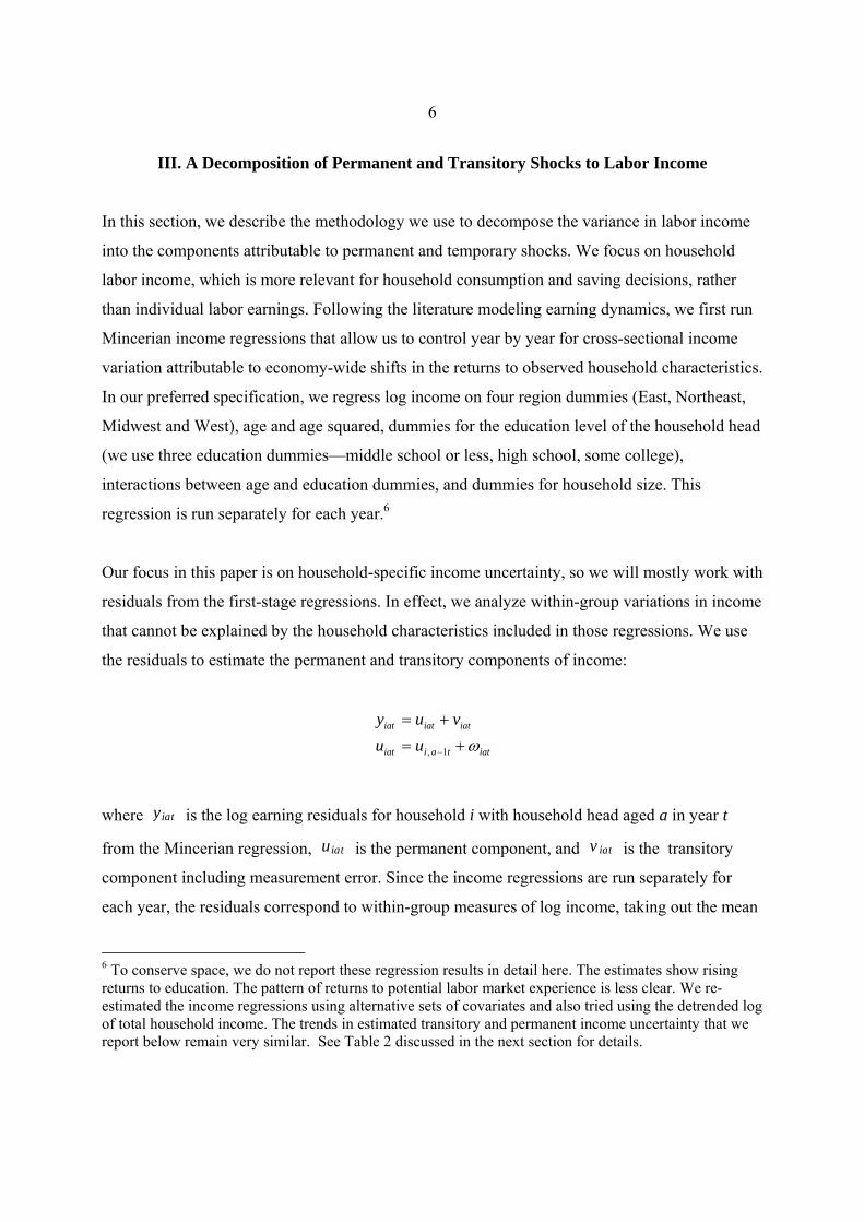
the residuals to estimate the permanent and transitory components of income:

iattaiiat

iatiatiat

uuvuyω+=

+=

−1,

where yiat is the log earning residuals for household i with household head aged a in year t

from the Mincerian regression, uiat is the permanent component, and v iat is the transitory

component including measurement error. Since the income regressions are run separately for

each year, the residuals correspond to within-group measures of log income, taking out the mean

6 To conserve space, we do not report these regression results in detail here. The estimates show rising returns to education. The pattern of returns to potential labor market experience is less clear. We re-estimated the income regressions using alternative sets of covariates and also tried using the detrended log of total household income. The trends in estimated transitory and permanent income uncertainty that we report below remain very similar. See Table 2 discussed in the next section for details.

7

effects of region, education level, age and the other household characteristics that we have

controlled for. The permanent shocks ω and transitory shocks v to earnings have zero means

and are mutually orthogonal. They are i.i.d. across household, time and age.7 We assume:

2

2

)var(

)var(

tiat

tiat

v ξ

ω

σ

σω

=

=

In other words, the variances of permanent and transitory shocks change by year but do not

depend on age. This in effect amounts to averaging over households with different ages (or in

different cohorts) in each year.8 Later, we will examine how these variances differ across age

groups. From here on, the subscript a will be dropped. The parameters to be estimated are: 2tξσ

and 2tωσ for each survey wave: }2009,2006,2004,2000,1997,1993,9119,1989{=t .

Suppose we observe household income in consecutive years. Identification hinges on the

variance and covariance structure of one-year changes in income:

21

22

211

211211

11

)var(

),cov(

−

−−

−−−−−−

−−

++=Δ

−=ΔΔ

−+=−=Δ−+=−=Δ

tttit

titit

itititititit

itititititit

y

yy

vvyyyvvyyy

ξξω

ξ

σσσ

σ

ωω

7 The transitory shocks do not appear to be serially correlated. We estimate the following autocovariances of unexplained income growth at lags 1 to 3 (standard errors in parentheses): -0.142 (0.016), 0.001 (0.017), 0.002 (0.018). Autocovariances of order 2 and higher are not statistically significant. If we test the null hypothesis of zero autocovariances in income growth (allowing autocovariances to be different across years), we reject the null hypothesis at lag one but not for higher order lags. These results indicate that the transitory shocks are either i.i.d or follow an MA(1) process. The latter is consistent with much of the literature (Abowd and Card, 1989; Meghir and Pistaferri, 2004; Blundell, Pistaferri and Preston, 2008). Because of the gaps between years of observations in the data, it is not possible to further test the stochastic process of transitory shocks. As we discuss later, the permanent uncertainty identified by our model is consistent regardless of whether the transitory shock follows an MA(1) process or is i.i.d. 8 We focus on the year effect and therefore the age and cohort effects cannot be separated. Given our sample size, we cannot allow variances to also vary by age (or cohort).

8

Thus, the one-period lagged autocovariance of income changes identifies the variance of the

transitory shock. With four years of data {t+1, t, t-1, t-2}, we would be able to identify 22

12 ,, ttt ξωω σσσ − . Note that the parameters are identified nonparametrically without making any

distributional assumptions about the shocks. Nor does the identification involve any assumption

about 2

0uσ , the initial variance of permanent earnings. This is an important advantage over

alternative identification strategies (e.g., moments using earning levels), particularly for a fast-

growing economy where 2

0uσ is likely to be nonstationary.

The uneven spacing of the CHNS waves complicates the analysis since we need to use n-year

rather one-year income changes:

204

206

205

206

200

204

201

202

203

204

292

293

291

293

292

293

206

204

200

297

293

291

)0406var(

)0004var(...

)8991,9193cov()9193,9397cov(

)9193var(

)0406,0609cov(

)0004,0406cov(

)9700,0004cov(

)9397,9700cov(

)9193,9397cov(

)8991,9193cov(

ξξωω

ξξωωωω

ωω

ξξωω

ξ

ξ

ξ

ξ

ξ

ξ

σσσσ

σσσσσσ

σσ

σσσσ

σ

σ

σ

σ

σ

σ

+++=−Δ

+++++=−Δ

−Δ−Δ−−Δ−Δ−+=

+++=−Δ

−=−Δ−Δ

−=−Δ−Δ

−=−Δ−Δ

−=−Δ−Δ

−=−Δ−Δ

−=−Δ−Δ

We are able to identify six years of the transitory income risk, all except 2009 and 1989. We do

not make any assumption about the transitory variances in those two years and, hence, we are

able to identify five permanent variances:

9

205

206

201

202

203

204

298

299

200

294

295

296

297

292

293

ωω

ωωωω

ωωω

ωωωω

ωω

σσ

σσσσ

σσσ

σσσσ

σσ

+

+++

++

+++

+

We estimate the model using an equally-weighted minimum distance estimator, a standard

approach in the literature since Moffitt and Gottschalk (1995). The model is just identified.

Note that our estimated variance of transitory shocks could be biased upwards for two reasons.

One is that in light of classical measurement errors (i.i.d.), the estimated variance of transitory

shocks will be inconsistent and biased upwards. This should not drive the trend in transitory

variance unless the variance of measurement errors itself has a trend. Second, we cannot exclude

the possibility that the transitory shocks may follow an MA(1) process (see footnote 7), implying

that the identified transitory variance also includes the transitory shocks from the previous year.

However, without additional assumptions, it is not possible to identify the MA(1) process given

the gaps between our sampling years. Since we are looking at n-year differences ( 2≥n ), even if

1−+= itititv θξξ (workers take two years to recover from a transitory shock to income), our

estimates of the variance of permanent shocks are still consistent. To see this:

)9193,9397cov()8991,9193cov(

)()()9193var(

)9193,9397cov(

)8991,9193cov(

292

293

292

2293

290

2291

292

293

292

2293

290

2291

−Δ−Δ−−Δ−Δ−+=

+++++=−Δ

−−=−Δ−Δ

−−=−Δ−Δ

ωω

ξξξξωω

ξξ

ξξ

σσ

σθσσθσσσ

σθσ

σθσ

In order to account for these two potential biases, when calibrating the savings model we will

assume that the true transitory uncertainty is only one-half of the transitory variance actually

identified from our estimates. This is a rather conservative assumption. Researchers using U.S.

household income data typically find that the estimated MA(1) parameter for the transitory shock

is small (between -0.1 to -0.2; see, e.g., Blundell, Pistaferri and Preston, 2008). So the upward

bias of the estimated transitory uncertainty due to serial correlation of the transitory shocks

10

( 21

2−tξσθ ) is likely to be small.

That leaves the potential bias from measurement errors. If we assume that measurement error

accounts for half of the identified transitory variance, then our estimates imply that measurement

error alone would explain more than 40 percent of the variance of income growth. In fact,

researchers conducting validation studies using U.S. data find that measurement error accounts

for only around a quarter of the variance of growth of earnings.9 It’s worth emphasizing that, so

long as the variance of the measurement error itself doesn’t have a trend, our estimates of the

trends in the variances of transitory and permanent shocks are still consistent.

IV. Earnings Decomposition Results

Table 2 reports, in panels A and B respectively, estimates of the variances of the permanent and

transitory shocks to household income and earnings over time. Standard errors are computed

using a block bootstrap procedure. One should bear in mind that the sample size is small, which

limits the power of statistical inference we are able to obtain (using the only available panel

dataset for the question we are interested in). The first column of panel A shows that, for the full

urban sample, there is no clear trend in the variance of permanent shocks to income. While the

point estimate increases from 0.012 to 0.030 from 1993 to 1997, the difference is not statistically

significant at the 5 percent level. The point estimate increases further to 0.043 in 2006, but the

difference relative to the estimate for 1993 is also not statistically significant.

Columns 2-7 provide the estimates based on alternative specifications for the Mincerian

regression. In column 2, we drop the age*education interaction terms. In column 3, we replace

household size fixed effects with fixed effects over the number of income earners. In column 4,

we use only a constant as a regressor. In column 5, we trim the sample to exclude households in

the top and bottom 1 percent of the distribution of raw household incomes. Finally, in columns 6

and 7, we restrict the sample to households headed by workers aged 30-60 years and 25-55 years,

9 See Bound and Krueger (1994). In the case of non-classical measurement errors, Pischke (1995) finds that the transitory variance is less contaminated due to the negative correlation of measurement errors with transitory earnings.

11

respectively. The results remain broadly the same across all these different specifications,

namely that there is no clear and statistically significant trend in the variance of permanent

shocks to income.

In Panel B of Table 2, we present estimates of the variance of transitory shocks to household

income. The point estimates in column 1 rise from 0.061 in 1991 to 0.181 by 2006, and this

increase is statistically significant at the 1% level.10 In other words, income uncertainty due to

transitory shocks to income almost triples from the beginning of the 1990s to the 2000s. A

similar pattern holds across the different specifications estimated in columns 2-7.

Table 3 presents the estimates from our baseline specification across different sub-samples. As in

the previous table, Panel A reports the estimates for the permanent variance. Column 1 reports

the estimates for the whole sample (and is identical to column 1 of Table 2). Column 2 reports

the estimates for a sample of households whose head worked in the SOCE sector when the

household entered the panel.11 The results are similar to those of column 1, and again do not

suggest any trend (and differences in point estimates between these two columns are not

statistically significant). When we split the sample by birth cohort (head born before or after

1955), the results remain broadly similar, suggesting no clear trend. Splitting the sample by

educational attainment of the household head (with or without high school degree) yields rather

noisy results, with large standard errors for the group of households with less-educated

household heads. This is in part driven by the large increase in education levels over the sample

(households with less educated heads are concentrated in the initial waves and those with more

educated heads in the most recent waves). But again, the estimates do not suggest a trend,

although they do suggest that the permanent uncertainty facing households with less-educated

heads is larger than the permanent uncertainty facing households with more educated heads.

Turning to the transitory variance (Panel B), the results are similar in the full and SOCE samples

10 The jump in transitory variance from 1991 to 1993 largely reflects a higher variance of raw log income in 1993 that partially settles back down in 1997 (this can also be seen in the jump in the standard deviation of household income in 1993 in Table 1). 11 The results are similar if we define the SOCE subsample based on SOCE employment throughout the survey (i.e., excluding workers who start in the SOCE sector but later move to the non-SOCE sector).

12

(columns 1 and 2), although the increase seems more gradual for the latter. The subsamples

where we divide observations by cohort and educational attainment of the household head have

noisier patterns, but are generally consistent with the trend of a substantial increase in the

variance of transitory shocks since the early 1990s. The pattern of a trend increase in transitory

uncertainty remains if we exclude transfers and subsidies from household income (last

column).12 In this case, the estimated level of uncertainty is generally higher in most years

compared to the level for total household income, consistent with the prior that transfers and

subsidies serve as partial insurance against idiosyncratic shocks to household income.

What accounts for the rising variance of transitory income shocks experienced by Chinese

households? While building a structural model to explain these facts is beyond the scope of this

paper, we provide some descriptive evidence from labor market turnover. A number of papers

have documented that higher labor market turnover (both job to job transitions and transition into

and out of unemployment) could lead to higher transitory uncertainty (see, e.g., Topel and Ward,

1992; Gottschalk and Moffitt, 1994). Gottschalk and Moffitt (2009) find that the rise in transitory

variance explains about half of the rise in cross-sectional income inequality in the U.S. through

the late 1980s and that this increase in earnings instability is in part attributable to greater

instability in jobs and higher labor market turnover.

Figure 3 shows that in urban China the transition rate from employment to unemployment for all

workers increases sharply in the late 1990s and continues to rise during the 2000s, corresponding

to the period when our estimates suggest that transitory income uncertainty began rising.13 The

transition from employment in the SOCE sector to employment in the non-SOCE sector is also

high starting in the mid-1990s, whereas the transition from non-SOCE employment to SOCE

sector employment has fallen. In addition to these labor market outcomes, the transition from a

centrally planned economy to a market economy may have resulted in an increase in firm-level 12 Transfers include both private and public transfers. Subsidies constitute firm-level nonwage compensation to the worker, and include subsidies on gas, food, education and housing as well as allowances for children. In the early stages of reform, SOCEs offered workers higher levels of subsidies to compensate for noncompetitive wages and then reduced them as their budget constraints were tightened (reduced transfers from the state to SOCE firms). The ratio of subsidies to total compensation was as high as 35 percent in the 1991 wave, but steadily declines to about 5 percent in the 2006 wave. 13 We define an individual as unemployed if he/she does not receive any wage or business income in a given year.

13

volatility related in part to state enterprise restructuring and a tighter link between wages and

firm-level performance. Wages paid to workers may be increasingly tied to firm performance

and more reflective of individual productivity due to tightening of budget constraints on SOCEs,

increased competition and more openness to foreign trade (see Groves, Hong, McMillan and

Naughton, 1994; Gang, Lunati and O’Connor, 1998; Benson and Zhu, 1999).

Comin, Groshen, and Rabin (2009) show that firm-level instability increased after 1980 in the

U.S. (particularly for large firms with volatile sales), corresponding to a period of higher

transitory variance of labor earnings documented in the U.S. Violante (2002) shows that skill-

neutral technological change could result in an increase in the variance of the transitory

component of earnings. In his model, workers learn vintage-specific skills and, when separating

from their jobs, can only partially transfer their skills across machines. Therefore, technological

acceleration reduces skill transferability and increases wage losses upon separation, which can

increase cross-sectional wage variability in an economy undergoing major technological shifts

and/or significant labor market churning. The rate of technological change in China since the

1990s has been even faster than in the U.S., due to the transition process and catching-up effects.

This makes skill-biased technological change a promising candidate to help explain the increase

in the variance of transitory income shocks.

V. Implications of the Shifts in Labor Income Variance for Precautionary Savings

Greater uncertainty in earnings at the microeconomic level can have macroeconomic

implications. One important channel is the impact of greater household-specific uncertainty on

precautionary savings. In the absence of a strong social safety net and an underdeveloped

financial system, this could lead households to self-insure by increasing their savings (Blanchard

and Giavazzi, 2006; Chamon and Prasad, 2010). In order to quantify the effects of this rise in

uncertainty on individual and aggregate savings, we now undertake a calibration of a

precautionary savings model, building on the work of Carroll (1997) and Gourinchas and Parker

(2002).14 This enables us to provide a quantitative measure of how the increase in the variance of

14 See also Fuchs-Schündeln (2008) and Kaplan and Violante (2010). Our calibration exercise sets only a lower bound on the degree of precautionary saving attributable to earnings uncertainty. We consider the

14

transitory shocks to household income can translate into the rise in savings among the younger

households observed in the data, while changes in pension rules can help explain the savings of

the older households.

A. Stylized Facts

To motivate this exercise, we turn again to Figure 2, which plots household saving rates as a

function of the age of the head of household observed in the actual data for different years, based

on the subsample of 10 provinces/municipalities used in Chamon and Prasad (2010).15 In the

early 1990s, the age-saving profile in China was fairly typical of those in other economies, with

saving rates increasing with age and then dropping off after retirement. Over time, savings rates

have increased across the board. But the increase is particularly pronounced for households with

relatively young household heads (those in their twenties and early thirties) and older household

heads (aged in the mid-fifties and up). Consequently, by 2005 the age-savings profile has an

unusual U-shaped pattern. Therefore, any empirically relevant explanation for the increase in

saving rates must account not only for the substantial average increase, but also for the unusual

way in which that increase was concentrated among the younger and older households. Our

calibration below is able to capture these empirically relevant features.

B. The Model and Calibration

We assume an instantaneous CRRA utility function, with individuals maximizing the expected

discounted flow of utility subject to a no-borrowing constraint:

max1

85

0 1

tt t

j ttj

Cs Eγ

βγ

−

=

⎛ ⎞ ⎡ ⎤⎜ ⎟ ⎢ ⎥−⎣ ⎦⎝ ⎠

∑ ∏

variance of different shocks to earnings only for workers who report positive earnings in each period. For workers who in reality face unemployment and the prospect of zero earnings, the precautionary savings motive could be even stronger. 15 The sample covers the following provinces: Anhui, Beijing, Chongqin, Ganshu, Guangdong, Hubei, Jiangsu, Liaoning, Shanxi and Sichuan. Only three of these overlap with the CHNS sample.

15

s.t. 1 (1 )( ), 0,t t t t tA r A Y C A t++ = + + − ≥ ∀

where β is the discount factor, s is an age-dependent survival probability, Ct is the level of

consumption in period t, γ is the coefficient of relative risk aversion, At is the level of assets, and

Yt represents income at time t. We assume that income is based on the same process estimated in

the previous section for the working years, but permanent income becomes deterministic in the

retirement period R at a particular fraction of the pre-retirement permanent income. That is:

1

t t t

t t t

y u vu u ω−

= += +

if t≤R

1

t t

t t

y uu u

η

−

==

if t>R

The model is solved backwards starting from the last period of life using the endogenous grid

point method developed by Carroll (2006). We calibrate the model assuming that working life

begins at age 25, with an initial level of wealth of zero and initial level of permanent income

equal to one. The discount factor β is 0.97. The real interest rate is 1.4 percent per annum, which

matches the average real interest rate in China over the period 1989-2006.16 The coefficient of

relative risk aversion γ is 4.5. We assume that economic agents live with certainty until the

retirement age of 60, have a survival probability until age 85, and die with certainty if still alive

at age 85. There are no bequests (for an individual who dies prior to age 85 with a positive level

of assets, those assets are “lost”).17

Permanent income in the retirement period is initially set such that η=75 percent of pre-

retirement permanent income, in line with the replacement rate prior to the 1997 reform. When

we model the effects of the pension reform (which affects workers retiring after 1997), we will

16 The real interest rate is based on the nominal interest rate on one-year bank deposits deflated by the annual CPI inflation rate. 17 For simplicity we assume a Poisson death process, calibrated to match life expectancy in China in 2009 (73.5 years). This results in a constant survival probability of 0.925 between t and t+1 after retirement.

16

set η=60.18

To calibrate the income process, we use the deterministic life-cycle growth rate of earnings in the

CHNS sample. We regress the log of family income on a complete set of cohort dummies,

household size, and a fourth-order polynomial in the age of the household head. We calculate the

marginal effect of age on household income at each age.19 The predicted annual income growth

is about 7 percent for the young, then ranges between 6 and 7 percent throughout most of the

remaining work life before gradually declining to 2 percent close to retirement age.

We want to model how saving rates respond to changes in income uncertainty along the lines

suggested by our empirical estimates in the previous section. We focus on family income and set

the variance of permanent shocks to income at a constant level of 0.02, while the variance of

transitory shocks goes from 0.04 in the baseline case up to 0.08. These variances are lower than

the point estimates reported in the earlier section on account of the conservative assumption we

make that half of the variance estimated in our empirical work is due to measurement error. This

assumption reduces the effect of rising uncertainty on saving in our calibrations. Moreover, by

not considering changes to the variance of permanent shocks, given the lack of a clear trend in

the empirical estimates, our calibration results provide a conservative assessment of how rising

uncertainty has affected savings.

C. Calibration Results

Figure 4A plots the simulated age profile of the saving rate. We construct the age-saving profile

by simulating the model for 5,000 households, and averaging their saving rates at each age. The

dashed line corresponds to the profile of savings under the initial baseline assumptions about the

variance of income. Consistent with this type of buffer-stock/life-cycle model, saving rates show

18 The replacement rate should decline over time, given the nature of the pension formula. Sin (2005) projects the replacement rate for a male retiring at age 60 to decline to about 60, 55 and 50 percent of the average wage by 2010, 2020 and 2030 respectively. Thus, our assumption for the decline in the replacement rate is a conservative one, particularly for younger workers. 19 This assumes that there is no cohort effect on the growth rate of earnings. That is, while younger cohorts are much richer than older ones, the age profile of income growth is the same for both. One could argue that younger cohorts should expect slower growth as China’s growth rate may eventually moderate.

17

a U-shaped pattern when plotted against age. Saving rates initially decline with age, since

households with the youngest household heads typically start their working life cycle with no

assets and need to save more in order to quickly build an adequate buffer stock of savings. Once

that buffer stock is built, savings remain relatively low until the late thirties/early forties when

earnings increase and life-cycle motives lead to a sharp increase in the savings rate.

The additional lines in this figure correspond to the age-saving profile after the change in the

income process. Each line corresponds to the saving behavior that would result if the regime

switch would occur starting at a given age of the household head (e.g. 25, 30,…, 55), and after

the initial jump we trace the behavior that would occur through the rest of the life cycle under

those parameters. That change is more easily seen in Figure 5B, which plots the change in the

saving rate after the shock as a function of the age of the household head. If a household head

were to begin working life at age 25 already under the higher uncertainty regime, that household

would save about 4.5 percentage points more to begin with. The difference in saving rates

relative to the baseline regime declines with age. For example, the initial jump for a household

with a forty year old head is only about 2.5 percentage points. The reason for this pattern is the

lower buffer stock of savings of the youngest households (since they start life with no buffer

stock of savings). A lower buffer stock causes households with younger heads to respond more

strongly to the shock to the transitory variance of income. The effect on households with older

heads is more muted because those households may already have accumulated a buffer stock of

savings. Incorporating an increase in the permanent variance of income would yield an even

stronger saving response by households with younger heads.

Figure 5 is analogous to Figure 4, but captures the shock to the pension replacement rate. The

initial baseline profile in Figure 5A is the same as in Figure 4A. The additional lines correspond

to simulated age-saving profiles following the decline in the retirement replacement ratio. Figure

5B plots the change in saving rates relative to that baseline. The change in the replacement ratio

induces a substantial increase in savings, particularly for households with older household heads

nearing retirement. After the pension reform, households need to save more in order to attain the

same level of post-retirement consumption as in the pre-reform scenario. The older the

household head, the less time there is to adjust life cycle savings to the lower replacement ratio

18

(i.e., compensate for past savings that were not made because the individual was living in a more

favorable pension environment). As a result, while the increase in the saving rate relative to the

pre-reform baseline is less than 1 percentage point for a household with a young household head

(in his or her early thirties), it is 5 percentage points for those with a household head in his or her

mid-forties, and as high as 8 percentage points for households with heads close to the end of their

working life.

In practice, the transition from the old to the new system was smoother than the discrete change

in our calibration, which therefore overstates the initial jump for the older workers. But note that

even the young households, which have plenty of time to adjust, will be saving over 5 percentage

points more by the time they approach retirement than they would have had under the old

pension regime. These long-run estimates are much less sensitive to the assumption of an initial

discrete change and indicate that, in the long term, households with older household heads will

continue to save substantially more than they used to in the past. It is also worth emphasizing

that the effect from pension reform could be amplified by the existence of income uncertainty.

Uncertain income streams during the household head’s working life leads to uncertainty about

pension benefits. With smaller anticipated pension benefits, this would lead to higher savings

even for households who have many years before retirement.

To jointly evaluate the effects of the rise in transitory income uncertainty as well as the change in

the pension replacement rate, in Figure 6 we show the results when both factors are introduced

simultaneously. As expected, saving rates respond more strongly once both shocks are

introduced, although the combined result is less than the sum of the two effects from Figures 4

and 5. The reason for this interaction is that the higher buffer-stock savings accumulated in

response to the increase in transitory earnings reduces the need for life-cycle savings later on

(and higher life-cycle savings also help protect against temporary shocks to income). There is a

marked increase in saving rates at the time of the switch, amounting to about 5 percentage points

for households with household heads in their twenties, thirties and forties. Saving rates tend to

decline after the initial jump for the younger households (since the main motive for the initial

jump is to quickly build up an adequate buffer stock). But for households with heads aged in the

mid-forties onwards, saving rates remain more stable (since the retirement motive is already

19

sufficiently strong). And as expected the initial jump (and subsequent saving behavior) is very

high for those with heads in their fifties, as those households have less time to adjust to a less

generous pension replacement rate.

The results from Figure 6 are informative but it is difficult to compare the increase in saving

rates from those plots with the increase observed in the cross-sectional data since saving rates in

the cross section involve a combination of the initial jumps as well as movements along the

curves over time. To facilitate that comparison, Figure 7 plots the change in cross-sectional

saving rates implied by the saving behavior in Figure 6 at different points in time relative to a

discrete increase in uncertainty and pension reform. The three lines indicate the change in the

cross-section at the time of the change and initial jump (t), as well as at t+5 and t+10 years,

which represent 5 and 10 year horizons, respectively, after the shifts in income uncertainty and

pensions.

Note that even though the envelope of the initial adjustment in savings increases with age in

Figure 4B (consistent with the change in the cross-section at time t), the movement along those

lines after the initial adjustment implies a U-shaped pattern for the change in savings in the

cross-section at t+5 and t+10. In all plots, the households with the youngest heads save about 5

percentage points more than they used to, while the oldest save 6.5 percentage points more at t+5

and 5.5 percentage points more at t+10. Both the t+5 and t+10 age profiles initially decline

rapidly with age, bottoming out at around 2.5 percentage points for households with heads

around age thirty or in their early thirties. In the t+10 cross-section, a household whose head is in

his or her early forties saves 3-4 percentage points more than before the reform, giving the cross-

sectional profile an asymmetric U-shaped pattern (with a relatively rapid initial decline followed

by a gradual increase in savings rates plotted against age of household head).

In short, our calibration of a standard buffer-stock/life-cycle model based on parameters taken

from our empirical estimation of the shifts in the variances of shocks to labor earnings, in

combination with estimates of the effects of the 1997 pension reform, can account for a sizable

increase in household saving rates and the U-shaped age-saving profile. Chamon and Prasad

(2010) trace much of the increase in the saving rates among the young to motives of saving for

20

housing purchases (about 6 percentage points for 25-29 year olds that do not own a home), and

among the old to health expenditures (about 6 percentage points for 55-59 year olds). Our

calibration exercise suggests that shifts in earnings uncertainty (including the effects of pension

reforms) played an important role as well.20 Our results would imply an even larger effect of

uncertainty if we were to consider a rise in the permanent variance. Even a modest increase in

the permanent variance can lead to a large increase in saving rates, with the effect being

particularly strong for households with younger household heads.

D. Robustness Checks

Preference Parameters

The simulated age profiles of consumption and savings depend critically on the preference

parameters--the coefficient of risk aversion and the discount factor--as well as on the expected

path for income growth. To examine the effects of deviations from the baseline values of the

preference parameters, we now simulate the changes in saving using various combinations of

these parameters.

Table 4 shows, for different values of key parameters, the simulated initial rise in saving rate for

different ages when there is both a rise in transitory uncertainty and a decline in the pension

replacement ratio as specified in the previous section. The first row is our baseline scenario,

shown in Figure 6. The second row assumes a larger decline in the pension replacement rate after

the reforms, down to a replacement ratio of 50 percent compared to 60 percent in our baseline.

As expected, that larger decline does not affect the households with youngest heads much on

impact (but will eventually affect their savings once they approach retirement), but leads to a

significantly larger response among households with older heads.

20 Housing motives for saving are not included in the calibration. If included, they would raise the saving rates of the younger individuals, accentuating the U-shaped age-saving profile and bringing it more in conformity with the pattern observed in savings data for Chinese urban households. Lumpy and uncertain health expenditures can still contribute to savings among the elderly (particularly among those that have already retired). But while the inclusion of both effects would further contribute to savings, the combined effect should be smaller than when each is considered in isolation (e.g., a higher buffer-stock accumulated in the aftermath of the pension reform can help older households better cope with health shocks).

21

The results in the remaining rows of Table 4 revert to our baseline assumptions for the increase

in uncertainty and pension reform, but show what happens when we vary the risk aversion and

discount factor parameters. Across a range of reasonable parameter values, the jump in saving

rates is on average broadly comparable to that in our baseline model (although the response for

the households with older heads tends to be larger). Lower risk aversion tends to reduce the

increase in savings for the young in response to the higher transitory uncertainty. Since a smaller

buffer stock is accumulated in the beginning of the life cycle, and at the same time consumers are

more willing to substitute away from current consumption towards future consumption, the

response to savings can be higher for other age groups for life cycle reasons. In cross-sectional

data, the increases in savings would result in a U-shaped age-saving profile after a few years due

to the rise in uncertainty and the decline in the replacement ratio.

In the penultimate row of Table 3, we calibrate the risk aversion parameter by fitting the

simulated age profile of the saving rate to the profile estimated empirically using data from the

Urban Household Survey (UHS, which reports income and consumption for different cross-

sections of households each year). For this calibration, the empirical cross-section of the saving

rates would not be appropriate, since it includes changes due to age, as well as cohort and year

effects, and variations in family composition. In order to calibrate the model, we need to estimate

the age profile of saving rates while controlling for those other effects.

We construct synthetic cohorts from different cross-sections of the UHS, and regress log income

and log consumption on a full set of dummies for age and cohort, and controls for family size

(including log of household size and the share of household members in different age groups).

But we restrict the sample to 1990-1997, since we are trying to calibrate the preference

parameters to match the saving behavior prior to the increase in uncertainty. Our estimated age

profile is based on the difference between the age effects for log income and the age effects for

log consumption.

We then calibrate the risk aversion parameter so as to match the mean saving rate for household

22

heads in seven age groups: 25-29, 30-34, …, and 55-59, using an identity weighting matrix.21

This matching exercise yields a coefficient of risk aversion of 8.1 and 7.5, when the discount

factor is set at 0.97 and 0.99, respectively. This high coefficient of risk aversion highlights the

challenges of explaining the high saving rates observed in China with a standard buffer-stock

life-cycle model of consumption. Given the combination of a generous pension replacement rate,

strong expected income growth and relatively low income risk, the only way for the model to

capture the high saving rate before 1997 is by setting the risk aversion parameter high enough to

reflect very risk-averse consumers. Presumably, more reasonable parameter values could match

the observed saving behavior if other saving motives were introduced (e.g., strong bequest and

housing motives, and the risk of lumpy health expenditures), which are beyond the scope of this

paper. Taking these parameters at face value, the model would still imply an increase in the

average saving rate of more than 2.5 percentage points. Note that the increase in savings for

households with young households heads is lower than under the baseline scenario, despite the

higher risk aversion. Since risk aversion is so high in this scenario, these households already save

a lot under the low uncertainty environment, reducing their need to adjust savings once

uncertainty rises (which also affects the other age ranges).

Even though it is difficult to explain the actual saving behavior of Chinese households with the

standard buffer-stock/life-cycle model, the estimates presented in this section are still useful and

informative. These results quantify how far this standard model would go, under reasonable

parameter values, towards explaining an increase in saving rates. Our calculations suggest that

about half of the increase observed during our sample could be explained by the rise in income

uncertainty and pension reform.

Expected Income Growth

Finally, we turn to the issue of how savings may be affected by an eventual slowdown in

21 The saving rates used for these seven age groups (from young to old) were: 23.0, 22.7, 21.1, 23.2, 25.9, 24.4 and 22.3 percent, respectively. This age-saving profile captures the estimated saving behavior for a household with a head aged 25 years in 1997 as he or she ages (not the 1997 cross-section of savings with respect to age). Note that this age-saving profile is not U-shaped as it is based on 1990-1997 data; the U-shaped profile does not appear in the data until the 2000s.

23

aggregate income growth in China. This could happen, for instance, if convergence effects stop

propelling growth in China or labor constraints due to demographic shifts reducef growth. Lower

income growth can decrease buffer-stock saving motives (as a lower saving rate is required for

the buffer-stock to keep up with permanent income). Lower income growth also reduces the

extent to which households postpone their retirement savings towards the end of their life cycle

(retirement savings are also affected by how income growth affects the expected retirement

period income).

Figure 8 plots, for different expected income growth scenarios, the age-savings profiles followed

by a household with a household head starting off at 25 years of age. Other than the expected

growth path, all plots assume the same parameters as in our baseline scenario under the higher

uncertainty and lower pension replacement ratio environment. The solid line corresponds to our

baseline expected growth path. The dotted line corresponds to a growth path that is 1 percentage

point lower than in our baseline from the present onwards. The dashed line is based on a growth

path where the expected income growth flattens out at a rate of 0.1 percentage point every year

relative to its value in our baseline path, but never declines below the lowest value in that path

(1.26 percent).22

The plots indicate that saving rates would be higher for households with young heads under both

lower income growth paths, more so when income slows down gradually (dashed line) than

when the decline takes place immediately (dotted line). The lower growth path substantially

reduces retirement income in our simulation, strengthening retirement saving motives and

causing households to save more even in the early stages of the life cycle. The age-savings

profile is flatter when the slowdown is gradual than when it takes place immediately. The age-

savings profile is steepest under our baseline expected growth path, where postponement of

retirement savings is strongest, and saving rates are actually higher in the working years close to

retirement age than under both alternative scenarios.

These results suggest that prospects of an eventual slowdown in Chinese growth could further 22 The income growth path includes the effects of trend income growth as well as age effects on income. Controlling for trend growth, income eventually declines with age, which explains this low value for household income growth despite the strong trend income growth.

24

increase household saving rates. Perhaps some of the savings observed among the very young

already take into account the prospects of income growth eventually slowing down. Song and

Yang (2010) make a similar point based on their results showing a flattening of age-earnings

profiles in the UHS data.

VI. Conclusion

In this paper, we analyzed a panel of urban Chinese households over the period 1989-2009 and

found that the variance of shocks to household income has increased over time and that the

increase is mainly accounted for by a rise in the variance of transitory shocks to income. This

increase in transitory uncertainty can help explain the rising saving rates among households with

younger household heads (who would need larger buffer stocks of savings to handle these

shocks). The pension reforms have led to a reduction in pension replacement income relative to

average wages for workers retiring after 1997. This cut in the pension replacement ratio can also

help explain rising saving rates, particularly for households with older household heads

approaching retirement—such households have less time to adjust to the change in pension

benefits and must therefore build up an adequate level of savings more quickly.

When we calibrate a standard buffer-stock life-cycle model of consumption with reasonable

parameter values, this riskier environment is capable of generating an initial increase of about

four and a half percentage points in the average household saving rate. Saving rates remain

significantly higher after that initial adjustment, with an average increase across age groups of

four and a half percentage points after 5 years. Moreover, this increase is concentrated among

households with household heads at the two ends of the age distribution in our sample. This

helps explain the unusual U-shaped age-profile of savings observed in urban China since the late

1990s.

Our calibration involved a number of assumptions for key parameters (e.g., how the pension

reform affected the replacement ratio). But we were systematically conservative in our

assumptions, erring on the side of downplaying the increase in these risks to income growth.

Nevertheless, our calibration of the standard buffer-stock life-cycle consumption model was still

25

capable of explaining half of the observed increase in savings among urban Chinese households,

while focusing only on this higher transitory variance of earnings and the 1997 pension reform.

These results may be helpful in thinking about policies to rebalance growth in China by boosting

private consumption and reducing the reliance on exports and investment to drive growth.

26

References Abowd, John, and David Card, 1989, “On the Covariance Structure of Earnings and Hours

Changes,” Econometrica, Vol. 57, No. 2, pp. 411-445. Bai, Chong-En, Jiangyong Lu, and Zhigang Tao, 2006, “The Multitask Theory of State

Enterprise Reform: Empirical Evidence from China,” American Economic Review, Vol. 96, No. 2, pp. 353-357.

Banerjee, Abhijit, Xin Meng, and Nancy Qian, 2010, “Fertility and Savings: Micro Evidence

from Family Planning in China,” Manuscript, MIT and Yale University. Baker, Michael, and Gary Solon, 2003, “Earnings Dynamics and Inequality Among Canadian

Men, 1976-1992: Evidence from Longitudinal Income Tax Records,” Journal of Labor Economics, Vol. 21, No. 2, pp. 289-321.

Benson, John, and Ying Zhu, 1999, “Markets, Firms and Workers In Chinese State-

Owned Enterprises,” Human Resource Management Journal, Vol. 9, No. 4, pp. 58–74. Blanchard, Olivier, and Francesco Giavazzi, 2006, “Rebalancing Growth in China: A Three-

handed Approach,” China and the World Economy, Vol. 14, No. 4, pp. 1-20. Blundell, Richard, Luigi Pistaferri, and Ian Preston, 2008, “Consumption Inequality and Partial

Insurance,” American Economic Review, Vol. 98, No. 5, pp. 1887-1921. Bound, John, and Alan Krueger, 1994, “The Extent of Measurement Error in Longitudinal

Earnings Data: Do Two Wrongs Make a Right?” Journal of Labor Economics, Vol. 9, pp. 1–24.

Brandt, Loren, Chang-Tai Hsieh, and Xiaodong Zhu, “Growth and Structural

Transformation in China,” in Loren Brandt and Thomas Rawski, eds., 2008, China’s Great Economic Transformation, Cambridge University Press.

Carroll, Christopher, 1997, “Buffer Stock Saving and the Life Cycle/Permanent Income

Hypothesis,” Quarterly Journal of Economics, Vol. 107, No. 1, pp. 1–56. Carroll, Christopher, 2006, “The Method of Endogenous Gridpoints for Solving Dynamic

Stochastic Optimization Problems,” Economics Letters, Vol. 91, No. 3, pp. 312–320. Carroll, Christopher, Jody Overland and David Weil, 2000, “Saving and Growth with Habit

Formation,” American Economic Review, Vol. 90, No. 3, pp. 341-355. Chamon, Marcos, and Eswar Prasad, 2010, “Why are Saving Rates of Urban Households in

China Rising?” American Economic Journal: Macroeconomics, Vol. 2, No. 1, pp. 93-130.

27

Comin, Diego, Erica L. Groshen and Bess Rabin, 2009, “Turbulent Firms, Turbulent Wages?” Journal of Monetary Economics, Vol. 56, No. 1, pp. 109-133.

Ding, Ning, and Yougui Wang, 2008, “Household Income Mobility in China and Its

Decomposition,” China Economic Review, Vol. 19, No. 3, pp. 373-380. Dunaway, Steven, and Vivek Arora, 2007, “Pension Reform in China: The Need for a New

Approach,” IMF Working Paper No. 07/109. Dwayne, Benjamin, Loren Brandt, and Jia-Zhueng Fan, 2003, “Ceaseless Toil? Health and

Labour Supply of the Elderly in Rural China,” Working Paper, University of Toronto. Feldstein, Martin, 1999, “Social Security Pension Reform in China,” China Economic Review,

Vol. 10, No. 2, pp. 99-107. Feng, Jing, Lixin He, and Hiroshi Sato, 2009, “Public Pension and Household Saving: Evidence

from China,” Bank of Finland BOFIT Discussion Paper 02/2009. Fuchs-Schündeln, Nicola, 2008, “The Response of Household Saving to the Large Shock of

German Reunification,” American Economic Review, Vol. 98, No. 5, pp. 1798-1828. Gang, Fan, Maria Rosa Lunati, and David O’Connor, 1998, “Labour Market Aspects of

State Enterprise Reform in China,” OECD Working Paper, No. 141. Gottschalk, Peter, and Robert Moffitt, 1994, “The Growth of Earnings Instability in the U.S.

Labor Market,” Brookings Papers on Economic Activity 2, pp. 217-272. Gottschalk, Peter, and Robert Moffitt, 2009, “The Rising Instability of U.S. Earnings,” Journal

of Economic Perspectives, Vol. 23, No. 4, pp. 3-24. Gourinchas, Pierre-Olivier, and Jonathan A. Parker, 2002, “Consumption Over the Life Cycle,”

Econometrica, Vol. 70, No. 1, pp. 47-89. Groves, Theodore, Yongmiao Hong, John McMillan and Barry Naughton, 1994,

“Autonomy and Incentives in Chinese State Enterprises,” The Quarterly Journal of Economics, Vol. 109, No. 1, pp. 183-209.

Herd, Richard, Hu-Wei Hu and Vincent Koen, 2010, “Providing Greater Old-Age Security in

China,” OECD Economics Department Working Papers, No. 750. Horioka, Charles Yuji, and Junmin Wan, 2007, “The Determinants of Household Saving in

China: A Dynamic Panel Analysis of Provincial Data,” Journal of Money, Credit, and Banking, Vol. 39, No. 8, pp. 2077-2096.

Kaplan, Greg, and Gianluca Violante, 2010, “How Much Consumption Insurance Beyond Self-

Insurance?” American Economic Journal: Macroeconomics, Vol. 2, No. 4, pp. 53-87.

28

Kraay, Aart, 2000, “Household Saving in China,” World Bank Economic Review, Vol. 14, No.3, pp. 545-70.

Kuijs, Louis, 2006, “How Will China’s Saving-Investment Balance Evolve?” World Bank Policy

Research Working Paper, No. 3958. Li, Weiye, and Louis Putterman, 2008, “Reforming China’s SOEs: An Overview,” Comparative

Economic Studies, Vol. 50, No. 3, pp. 353-380. Li, Hongbin, and Yi Zhu 2006, “Income, Income Inequality, and Health: Evidence from China,”

Journal of Comparative Economics, Vol. 34, No. 4, pp. 668-693 Lillard, Lee A., and Yoram Weiss, 1979, “Components of Variation in Panel Earnings Data:

American Scientists, 1960–70,” Econometrica, Vol. 47, No. 2, pp. 437–54. Lin, Justin Yifu, Fang Cai, and Zhou Li, 1998, “Competition, Policy Burdens, and State-Owned

Enterprise Reform,” American Economic Review, Vol. 88, No. 2, pp. 422-427. MaCurdy, Thomas E., 1982, “The Use of Time Series Processes to Model the Error Structure of

Earnings in Longitudinal Data Analysis,” Journal of Econometrics, Vol. 18, No. 1, pp. 83–114.

Meng, Xin, 2003, “Unemployment, Consumption Smoothing, and Precautionary Saving in

Urban China,” Journal of Comparative Economics, Vol. 31, No. 3, pp. 465-485. Meghir, Costas, and Luigi Pistaferri, 2004, “Income Variance Dynamics and Heterogeneity,”

Econometrica, Vol. 72, No. 1, pp. 1-32. Modigliani, Franco, and Shi Larry Cao, 2004, “The Chinese Saving Puzzle and the Life Cycle

Hypothesis,” Journal of Economic Literature, Vol. 42, pp. 145-70. Moffitt, Robert, and Peter Gottschalk, 1995, “Trends in the Transitory Variance of Male

Earnings in the U.S, 1970-1987,” Mimeo, Johns Hopkins University. Moffitt, Robert, and Peter Gottschalk, 2009, “Trends in the Transitory Variance of Male

Earnings in the U.S., 1970-2004,” Mimeo, Johns Hopkins University. Pischke, Jorn-Steffen, 1995, “Measurement Error and Earnings Dynamics: Some Estimates From

the PSID Validation Study,” Journal of Business and Economic Statistics, Vol. 13, No. 3, pp. 305-314.

Qian, Yingyi, 1998, “Urban and Rural Household Saving in China,” IMF Staff Papers, Vol. 35,

No. 4, pp. 592-627. Sin, Yvonne, 2005, “Pension Liabilities and Reform Options for Old Age Insurance,” World

Bank Working Paper No. 2005-1.

29

Song, Michael, and Dennis Yang, 2010, “Life Cycle Earnings and the Household Saving Puzzle in a Fast-Growing Economy” Manuscript, Chinese University of Hong Kong.

Topel, Robert H., and Michael P. Ward, 1992, “Job Mobility and the Careers of Young Men,”

Quarterly Journal of Economics, Vol. 107, No. 2, pp. 439-79. Violante, Gianluca, 2002, “Technological Acceleration, Skill Transferability, and the Rise in

Residual Inequality,” Quarterly Journal of Economics, Vol. 117, No. 1, pp. 297-338. Wei, Shang-Jin, and Xiaobo Zhang, 2011, “The Competitive Saving Motive: Evidence from

Rising Sex Ratios and Savings Rates in China,” Journal of Political Economy, Vol. 119, No. 3, pp. 511-64.

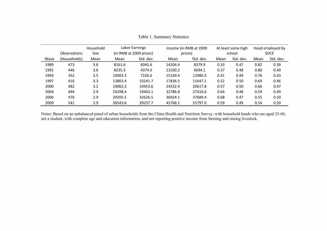
Table 1. Summary Statistics

   Observations Household 

Size Labor Earnings  Income (in RMB at 2009 

prices)  At least some high 

school Head employed by 

SOCE (in RMB at 2009 prices) Wave  (Households)  Mean  Mean  Std. dev.  Mean  Std. dev.  Mean  Std. dev.  Mean  Std. dev. 1989  473  3.8  8161.6  6045.6  14204.4  8379.9  0.33  0.47  0.82  0.39 1991  446  3.6  8235.3  4374.0  13100.2  6694.1  0.37  0.48  0.80  0.40 1993 352  3.5 10003.3 7226.6 15169.4  12985.5 0.41 0.49 0.76 0.431997  416  3.3  13803.4  10241.7  17836.5  11647.1  0.52  0.50  0.69  0.46 2000  482  3.2  19062.3  19453.6  24332.4  20617.8  0.57  0.50  0.66  0.47 2004  494  2.9  24298.4  19403.1  32786.8  27418.6  0.64  0.48  0.59  0.49 2006  476  2.9  29205.5  32626.5  36924.1  37689.4  0.68  0.47  0.55  0.50 2009  541  2.9  36543.6  39237.7  45766.1  55797.0  0.59  0.49  0.54  0.50 

Notes: Based on an unbalanced panel of urban households from the China Health and Nutrition Survey, with household heads who are aged 25-60, not a student, with complete age and education information, and not reporting positive income from farming and raising livestock.

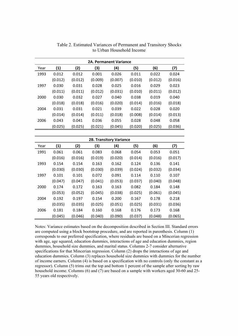
Table 2. Estimated Variances of Permanent and Transitory Shocks to Urban Household Income

2A. Permanent Variance 

Year  (1)  (2)  (3)  (4)  (5)  (6)  (7) 1993  0.012  0.012  0.001  0.026  0.011  0.022  0.024 

(0.012)  (0.012)  (0.009)  (0.007)  (0.010)  (0.012)  (0.016) 1997  0.030  0.031  0.028  0.025  0.016  0.029  0.023 

(0.011)  (0.011)  (0.012)  (0.031)  (0.010)  (0.011)  (0.012) 2000  0.030  0.032  0.027  0.040  0.038  0.019  0.040 

(0.018)  (0.018)  (0.016)  (0.020)  (0.014)  (0.016)  (0.018) 2004  0.031  0.031  0.021  0.039  0.022  0.028  0.020 

(0.014)  (0.014)  (0.011)  (0.018)  (0.008)  (0.014)  (0.013) 2006  0.043  0.041  0.036  0.055  0.028  0.048  0.058    (0.025)  (0.025)  (0.021)  (0.045)  (0.020)  (0.025)  (0.036) 

                       

2B. Transitory Variance 

Year  (1)  (2)  (3)  (4)  (5)  (6)  (7) 

1991  0.061  0.061  0.083  0.068  0.054  0.053  0.051 (0.016)  (0.016)  (0.019)  (0.020)  (0.014)  (0.016)  (0.017) 

1993  0.154  0.154  0.163  0.162  0.124  0.136  0.141 (0.030)  (0.030)  (0.030)  (0.039)  (0.024)  (0.032)  (0.034) 

1997  0.101  0.101  0.072  0.091  0.114  0.110  0.107 (0.047)  (0.047)  (0.041)  (0.053)  (0.037)  (0.040)  (0.048) 

2000  0.174  0.172  0.163  0.163  0.082  0.184  0.148 (0.053)  (0.052)  (0.045)  (0.038)  (0.025)  (0.061)  (0.045) 

2004  0.192  0.197  0.154  0.200  0.167  0.178  0.218 (0.035)  (0.035)  (0.025)  (0.051)  (0.025)  (0.031)  (0.036) 

2006  0.181  0.184  0.160  0.168  0.176  0.173  0.168    (0.045)  (0.046)  (0.040)  (0.090)  (0.037)  (0.048)  (0.065) 

Notes: Variance estimates based on the decomposition described in Section III. Standard errors are computed using a block bootstrap procedure, and are reported in parenthesis. Column (1) corresponds to our preferred specification, where residuals are based on a Mincerian regression with age, age squared, education dummies, interactions of age and education dummies, region dummies, household size dummies, and marital status. Columns 2-7 consider alternative specifications for that Mincerian regression. Column (2) drops the interactions of age and education dummies. Column (3) replaces household size dummies with dummies for the number of income earners. Column (4) is based on a specification with no controls (only the constant as a regressor). Column (5) trims out the top and bottom 1 percent of the sample after sorting by raw household income. Columns (6) and (7) are based on a sample with workers aged 30-60 and 25-55 years old respectively.

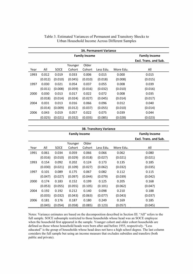
Table 3. Estimated Variances of Permanent and Transitory Shocks to Urban Household Income Across Different Samples

3A. Permanent Variance 

Family Income  Family Income 

Excl. Trans. and Sub. 

Year  All  SOCE Younger Cohort 

Older Cohort  Less Edu.  More Edu.  All 

1993  0.012  0.019  0.033  0.006  0.015  0.000  0.015 (0.012)  (0.010)  (0.045)  (0.010) (0.018)  (0.008)  (0.015) 

1997  0.030  0.021  0.054  0.037  0.055  0.008  0.039 (0.011)  (0.008)  (0.059)  (0.016) (0.032)  (0.010)  (0.016) 

2000  0.030  0.013  0.017  0.022  0.072  0.008  0.035 (0.018)  (0.014)  (0.024)  (0.027) (0.045)  (0.014)  (0.017) 

2004  0.031  0.013  0.016  0.066  0.096  0.012  0.040 (0.014)  (0.009)  (0.012)  (0.037) (0.055)  (0.010)  (0.014) 

2006  0.043  0.019  0.057  0.022  0.075  0.039  0.044 

   (0.025)  (0.021)  (0.032)  (0.035) (0.085)  (0.028)  (0.023) 

                       

3B. Transitory Variance

Family Income  Family Income 

   Excl. Trans. and Sub. 

Year  All  SOCE Younger Cohort 

Older Cohort  Less Edu.  More Edu.  All 

1991  0.061  0.034  0.059  0.066  0.066  0.062  0.080 (0.016)  (0.010)  (0.029)  (0.018) (0.027)  (0.021)  (0.021) 

1993  0.154  0.092  0.202  0.124  0.173  0.135  0.185 (0.030)  (0.021)  (0.109)  (0.027) (0.062)  (0.032)  (0.035) 

1997  0.101  0.089  0.175  0.067  0.082  0.112  0.115 (0.047)  (0.027)  (0.097)  (0.044) (0.079) (0.039) (0.042) 

2000  0.174  0.183  0.152  0.199 0.125 0.205 0.168 (0.053)  (0.055)  (0.055)  (0.105) (0.101) (0.062) (0.047) 

2004  0.192  0.192  0.212  0.140  0.098  0.210  0.188 (0.035)  (0.032)  (0.043)  (0.063) (0.077)  (0.043)  (0.037) 

2006  0.181  0.176  0.187  0.180  0.249  0.169  0.185 

   (0.045)  (0.054)  (0.058)  (0.085) (0.123)  (0.057)  (0.045) 

Notes: Variance estimates are based on the decomposition described in Section III. “All” refers to the full sample. SOCE subsample restricted to those households whose head was an SOCE employee when the household first appeared in the sample. Younger cohort and older cohort households are defined as those whose household heads were born after and before 1955, respectively. “Less educated” is the group of households whose head does not have a high school degree. The last column considers the full sample but using an income measure that excludes subsidies and transfers (both public and private).

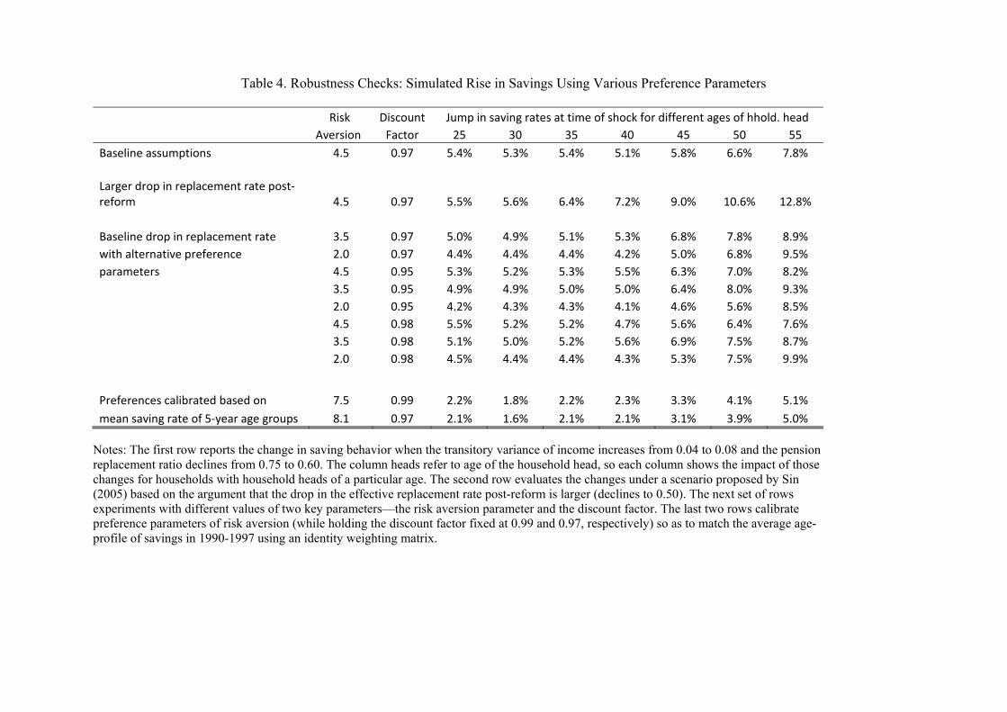
Table 4. Robustness Checks: Simulated Rise in Savings Using Various Preference Parameters

Risk   Discount  Jump in saving rates at time of shock for different ages of hhold. head    Aversion   Factor  25  30  35  40  45  50  55 Baseline assumptions  4.5  0.97  5.4%  5.3%  5.4%  5.1%  5.8%  6.6%  7.8%                    Larger drop in replacement rate post‐reform  4.5  0.97  5.5%  5.6%  6.4%  7.2%  9.0%  10.6%  12.8%                    Baseline drop in replacement rate   3.5  0.97  5.0%  4.9%  5.1%  5.3%  6.8%  7.8%  8.9% with alternative preference   2.0  0.97  4.4%  4.4%  4.4%  4.2%  5.0%  6.8%  9.5% parameters  4.5  0.95  5.3%  5.2%  5.3%  5.5%  6.3%  7.0%  8.2%   3.5  0.95  4.9%  4.9%  5.0%  5.0%  6.4%  8.0%  9.3%   2.0  0.95  4.2%  4.3%  4.3%  4.1%  4.6%  5.6%  8.5%   4.5  0.98  5.5%  5.2%  5.2%  4.7%  5.6%  6.4%  7.6%   3.5  0.98  5.1%  5.0%  5.2%  5.6%  6.9%  7.5%  8.7%   2.0  0.98  4.5%  4.4%  4.4%  4.3%  5.3%  7.5%  9.9% 

Preferences calibrated based on   

7.5  0.99  2.2%  1.8%  2.2%  2.3%  3.3%  4.1%  5.1% 

mean saving rate of 5‐year age groups  8.1  0.97  2.1%  1.6%  2.1%  2.1%  3.1%  3.9%  5.0%  Notes: The first row reports the change in saving behavior when the transitory variance of income increases from 0.04 to 0.08 and the pension replacement ratio declines from 0.75 to 0.60. The column heads refer to age of the household head, so each column shows the impact of those changes for households with household heads of a particular age. The second row evaluates the changes under a scenario proposed by Sin (2005) based on the argument that the drop in the effective replacement rate post-reform is larger (declines to 0.50). The next set of rows experiments with different values of two key parameters—the risk aversion parameter and the discount factor. The last two rows calibrate preference parameters of risk aversion (while holding the discount factor fixed at 0.99 and 0.97, respectively) so as to match the average age-profile of savings in 1990-1997 using an identity weighting matrix.

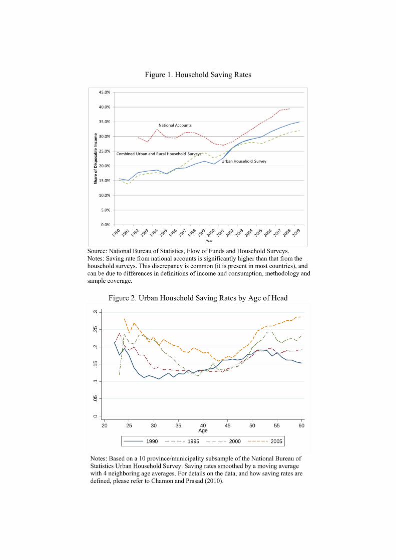
Figure 1. Household Saving Rates

0.0%

5.0%

10.0%

15.0%

20.0%

25.0%

30.0%

35.0%

40.0%

45.0%Share of Dispo

sable Income

Year

National Accounts

Urban Household Survey

Combined Urban and Rural Household  Surveys

Source: National Bureau of Statistics, Flow of Funds and Household Surveys. Notes: Saving rate from national accounts is significantly higher than that from the household surveys. This discrepancy is common (it is present in most countries), and can be due to differences in definitions of income and consumption, methodology and sample coverage.

Figure 2. Urban Household Saving Rates by Age of Head

0.0

5.1

.15

.2.2

5.3

20 25 30 35 40 45 50 55 60Age

1990 1995 2000 2005

Notes: Based on a 10 province/municipality subsample of the National Bureau of Statistics Urban Household Survey. Saving rates smoothed by a moving average with 4 neighboring age averages. For details on the data, and how saving rates are defined, please refer to Chamon and Prasad (2010).

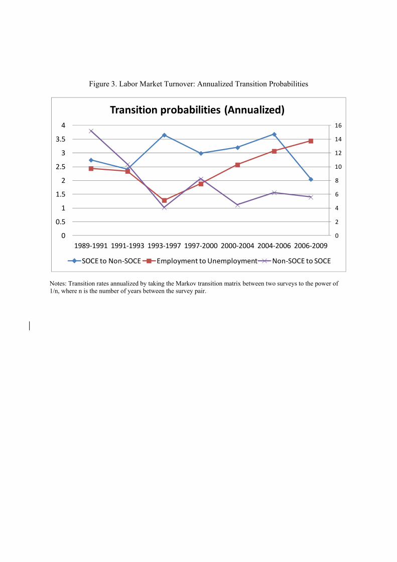
Figure 3. Labor Market Turnover: Annualized Transition Probabilities

0

2

4

6

8

10

12

14

16

0

0.5

1

1.5

2

2.5

3

3.5

4

1989‐1991 1991‐1993 1993‐1997 1997‐2000 2000‐2004 2004‐2006 2006‐2009

Transition probabilities (Annualized)

SOCE to Non‐SOCE Employment to Unemployment Non‐SOCE to SOCE

Notes: Transition rates annualized by taking the Markov transition matrix between two surveys to the power of 1/n, where n is the number of years between the survey pair.

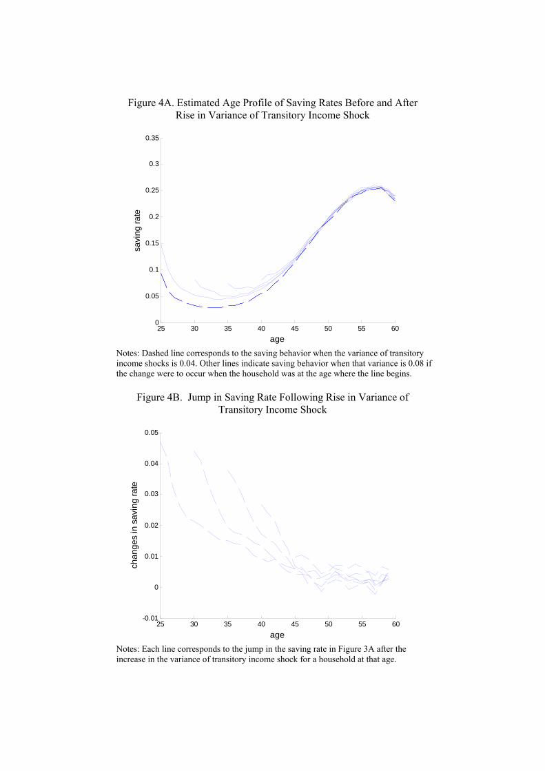
Figure 4A. Estimated Age Profile of Saving Rates Before and After Rise in Variance of Transitory Income Shock

25 30 35 40 45 50 55 600

0.05

0.1

0.15

0.2

0.25

0.3

0.35

age

savi

ng ra

te

Notes: Dashed line corresponds to the saving behavior when the variance of transitory income shocks is 0.04. Other lines indicate saving behavior when that variance is 0.08 if the change were to occur when the household was at the age where the line begins.

Figure 4B. Jump in Saving Rate Following Rise in Variance of

Transitory Income Shock

25 30 35 40 45 50 55 60-0.01

0

0.01

0.02

0.03

0.04

0.05

age

chan

ges

in s

avin

g ra

te

Notes: Each line corresponds to the jump in the saving rate in Figure 3A after the increase in the variance of transitory income shock for a household at that age.

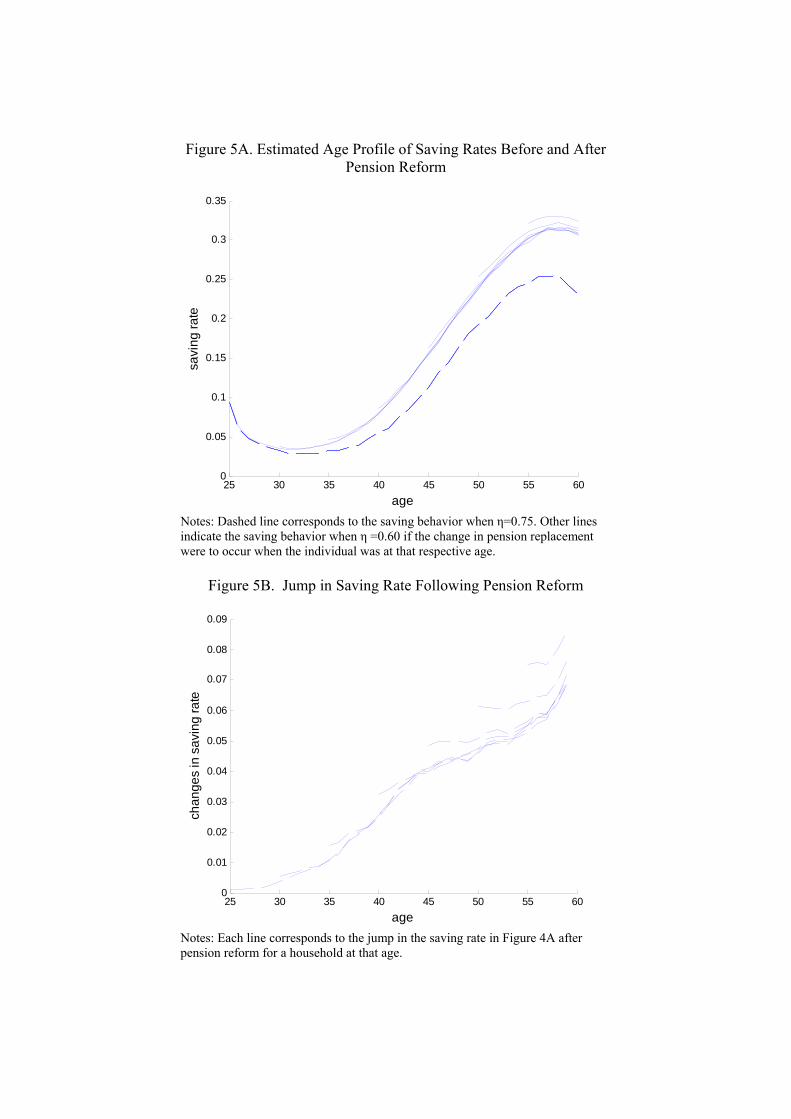
Figure 5A. Estimated Age Profile of Saving Rates Before and After Pension Reform

25 30 35 40 45 50 55 600

0.05

0.1

0.15

0.2

0.25

0.3

0.35

age

savi

ng ra

te

Notes: Dashed line corresponds to the saving behavior when η=0.75. Other lines indicate the saving behavior when η =0.60 if the change in pension replacement were to occur when the individual was at that respective age.

Figure 5B. Jump in Saving Rate Following Pension Reform

25 30 35 40 45 50 55 600

0.01

0.02

0.03

0.04

0.05

0.06

0.07

0.08

0.09

age

chan

ges

in s

avin

g ra

te

Notes: Each line corresponds to the jump in the saving rate in Figure 4A after pension reform for a household at that age.

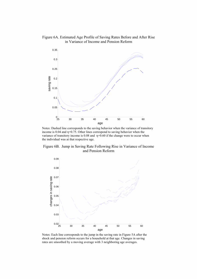
Figure 6A. Estimated Age Profile of Saving Rates Before and After Rise in Variance of Income and Pension Reform

25 30 35 40 45 50 55 600

0.05

0.1

0.15

0.2

0.25

0.3

0.35

age

savi

ng ra

te

Notes: Dashed line corresponds to the saving behavior when the variance of transitory income is 0.04 and η=0.75. Other lines correspond to saving behavior when the variance of transitory income is 0.08 and η=0.60 if the change were to occur when the individual was at that respective age.

Figure 6B. Jump in Saving Rate Following Rise in Variance of Income

and Pension Reform

25 30 35 40 45 50 55 600.02

0.03

0.04

0.05

0.06

0.07

0.08

0.09

age

chan

ges

in s

avin

g ra

te

Notes: Each line corresponds to the jump in the saving rate in Figure 5A after the shock and pension reform occurs for a household at that age. Changes in saving rates are smoothed by a moving average with 3 neighboring age averages.

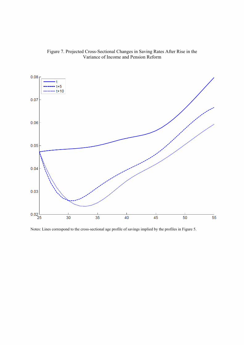
Figure 7. Projected Cross-Sectional Changes in Saving Rates After Rise in the

Variance of Income and Pension Reform

Notes: Lines correspond to the cross-sectional age profile of savings implied by the profiles in Figure 5.

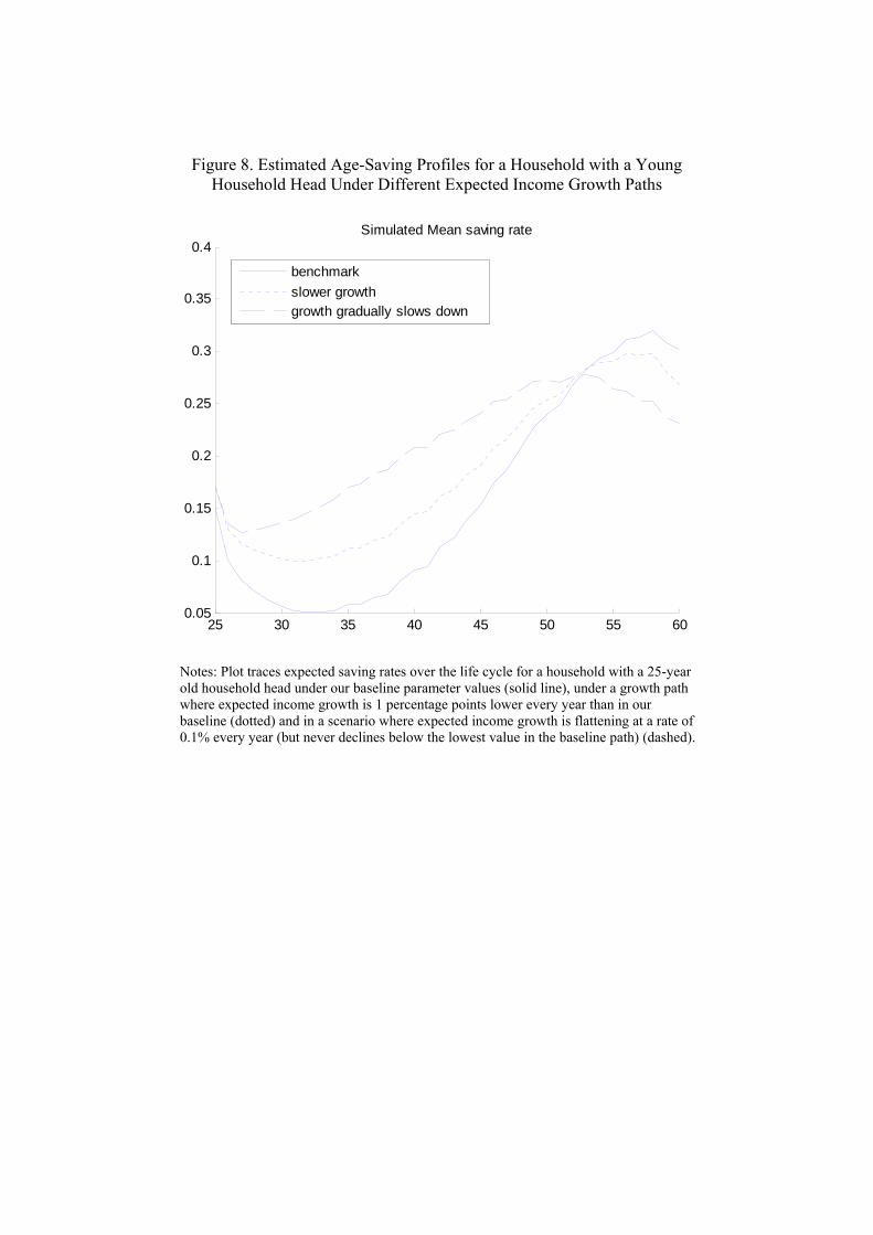
Figure 8. Estimated Age-Saving Profiles for a Household with a Young Household Head Under Different Expected Income Growth Paths

25 30 35 40 45 50 55 600.05

0.1

0.15

0.2

0.25

0.3

0.35

0.4Simulated Mean saving rate

benchmarkslower growth growth gradually slows down

Notes: Plot traces expected saving rates over the life cycle for a household with a 25-year old household head under our baseline parameter values (solid line), under a growth path where expected income growth is 1 percentage points lower every year than in our baseline (dotted) and in a scenario where expected income growth is flattening at a rate of 0.1% every year (but never declines below the lowest value in the baseline path) (dashed).