Atmospheric Environment 38 (2004) 1801–1809

ARTICLE IN PRESS

*Correspond

E-mail addr

1352-2310/$ - se

doi:10.1016/j.at

Improved method ‘‘grid translation’’ for mappingenvironmental pollutants using a two-dimensional CAT

scanning system

Wim Verkruysse, Lori A. Todd*

Department of Environmental Sciences and Engineering, University of North Carolina at Chapel Hill, Chapel Hill, NC 27599, USA

Received 10 August 2003; accepted 24 November 2003

Abstract

This research reports on a new method that improves two-dimensional tomographic mapping of air pollutants. In

traditional reconstruction techniques, a single grid of cells was used to reconstruct a two-dimensional map from

measured line integrated open-path Fourier transform infrared (OP-FTIR) spectrometer measurements. Typically, in

environmental two-dimensional imaging, the area of interest is sparsely sampled with rays. As a result, the

reconstruction grid resolution has to be coarse in order to avoid grid cells that are hit by very few rays. Unfortunately,

successful reconstruction of a peak on a coarse grid depends on its position with respect to a grid cell. If it lies mostly

within one grid cell, the reconstructed peak value will be fairly accurate; if it overlaps two or more cells, the predicted

concentrations are lower. On average, this leads to an underestimation of the peak value, as well as a strong variability

when a peak changes location or when a different reconstruction resolution is selected. This paper presents a recently

developed ‘‘grid translation’’ method that allows the choice of the reconstruction resolution to be less critical than using

previous single grid methods. In addition, this method substantially improves the quantitative and qualitative

reconstruction accuracy of concentration maps under the configuration constraints of OP-FTIR CAT scanning

systems.

r 2004 Elsevier Ltd. All rights reserved.

Keywords: FTIR spectroscopy; Chemical imaging; Reconstruction; Computed tomography; Exposure assessment

1. Introduction

Current techniques for monitoring chemical emissions

indoors or outdoors use time-integrated or real-time

point sampling devices placed at specific and isolated

locations throughout an area. These isolated measure-

ments provide information only about chemicals emitted

at a specific time period and for a specific location. If

time-integrated methods are used, information concern-

ing short-term peaks of concentrations is lost. In any

case, data is confined to a small spatial region and

scientists are forced to estimate chemical concentrations

ing author. Fax: +1-919-966-4711.

ess: todd@cs.unc.edu (L.A. Todd).

e front matter r 2004 Elsevier Ltd. All rights reserve

mosenv.2003.11.039

in the unsampled regions. The isolated data points do

not provide an overall understanding of chemical

generation and transport over time and space.

An innovative method has been developed that

creates, in real-time, two-dimensional maps of chemical

contaminants in air. With these maps, scientists can

resolve the concentration and dispersion patterns of

multiple chemicals with good spatial and temporal

resolution. The technology used in this mapping method

combines the measurement techniques of optical remote

sensing with the mapping capabilities of computer-

assisted tomography (CAT) to provide accurate spatial

and temporal information about contaminant concen-

trations and dispersion patterns (Yost et al., 1994;

Drescher et al., 1996; Todd et al., 2001). CAT is best

d.

ARTICLE IN PRESSW. Verkruysse, L.A. Todd / Atmospheric Environment 38 (2004) 1801–18091802

known for its use in medicine (Hounsfield, 1973;

Cormack, 1964). The first discussions of applying CAT

to air pollution were by Byer and Shepp (1979) and

Wolfe and Byer (1979) who described a theoretical laser-

based system used on an urban scale. CAT was

proposed initially by Todd and Leith (1990) to measure

pollutants in indoor air and it has since been evaluated

in theoretical, experimental and outdoor field studies. It

has been deployed in the field to calculate emission rates

of ammonia from a 6-acre swine waste lagoon (Todd

et al., 2001). In theory, this method could be used to

map a variety of areas, from a small room up to an area

over 300 km on a side.

For environmental and industrial applications, open-

path Fourier transform infrared (OP-FTIR) spectro-

meters have been primarily used as the optical remote

sensing device in the system; however, other open-path

instruments such as tunable diode lasers could be used

as well (Warland et al., 2001). The OP-FTIR spectro-

meters scan the air in near-real time by non-invasively

sampling across a long open-space; each single beam of

infrared light probes the air, measuring the attenuation

of light from chemical contaminants and returns a path-

integrated concentration of chemicals. Thus, chemicals

are measured over a path, not at a single point.

With the use of multiple spectrometers, a non-invasive

network of intersecting path-integrated concentrations

are obtained, all within a horizontal slice of air in the

area of interest. Tomographic reconstruction algorithms

are used to transform the network of concentrations into

a spatially resolved, two-dimensional concentration map

over the plane that is sampled. The spatial resolution of

this environmental CAT scanning system enables non-

uniform sources to be measured. Each map provides a

snapshot, which represents a short period of measure-

ment (minutes), of the concentrations and locations of

multiple chemicals in air. As new maps are obtained

over time, the reconstructed concentration maps are

linked together to visualize the flow of contaminants

over both space and time. This provides a powerful tool

for evaluating chemical dispersion, emission and ex-

posure. These maps allow spatial and temporal resolu-

tion to be obtained using far fewer instruments than

would be necessary to obtain the same level of detail

using point sampling devices.

Ideally, to capture an accurate and spatially resolved

profile of concentrations, a high density of optical rays

would be taken simultaneously; the higher the density of

rays, the higher the reconstruction resolution. In

practice, with the current OP-FTIR spectrometer

technology, multiple optical rays are taken sequentially

in time over a given period. Therefore, for mapping

fluctuating chemical concentrations, because sequential

open-path measurements are obtained, the overall

sampling time must be kept to a minimum. This is

accomplished through a combination of limiting the

individual sampling time for a single ray and limiting the

number of total OP-FTIR spectrometer rays. This can

compromise both the accuracy and resolution of the

final concentration maps.

When the density of rays is sparse, a coarse (low

resolution) map is reconstructed. The resolution of a

map relates to the number of grid cells (or squares) that

a map contains which translates into the spatial

resolution of concentrations for an area. The higher

the number of grid cells in a map, the higher the spatial

resolution. When reconstructing chemical concentra-

tions, the selection of the spatial resolution has

depended upon the given application, the number of

optical rays and spectrometers, and the expected

chemical concentration profile. While the spatial resolu-

tion of a map depends on multiple factors, to accurately

reconstruct the concentrations in a grid cell, usually a

minimum of one or two OP-FTIR spectrometer rays

must cross the cell. The grid cell size is usually

determined by theoretical tests that include the para-

meters listed above. For practical purposes, a fixed

single grid cell size must be selected in order to

reconstruct the maps; however, a single grid cell size

can also impact the accuracy of some of the concentra-

tion estimates.

This paper presents a recently developed ‘‘grid

translation’’ method that allows the choice of the

reconstruction resolution to be less critical than using

previous methods. In addition, this method substantially

improves the quantitative and qualitative reconstruction

accuracy of concentration maps under the configuration

constraints of OP-FTIR CAT scanning systems. Results

using the grid translation method are compared with the

conventional single grid method by reconstructing test

maps from computer simulated concentration data using

the maximum likelihood with expectation maximization

(MLEM) algorithm. The reconstructed concentration

maps were evaluated using different quantitative mea-

sures of image quality.

2. Theory and methodology

2.1. Reconstruction algorithm

The MLEM tomographic reconstruction algorithm

was used in this study to reconstruct the path-integrated

measurements (Tsui et al., 1991; Shepp and Vardi, 1982;

Samanta and Todd, 2000). To reconstruct a concentra-

tion map, an idealized area was broken into an N�M

square or rectangular grid of cells. The concentration in

each cell was assumed to be homogeneous, non-

negative, and was updated with each iteration. Within

each grid cell, the MLEM algorithm iteratively updated

concentrations in the N�M grid cells by comparing a

set of measured path-integrated ray sums with a set of

ARTICLE IN PRESSW. Verkruysse, L.A. Todd / Atmospheric Environment 38 (2004) 1801–1809 1803

calculated path-integrated ray sums. The process was

terminated after a pre-determined number of iterations.

Fifty iterations were used for this research. The

calculated ray sums were obtained according to

Eq. (1). The concentrations Cqi were updated in each

iteration step according to Eq. (2).

pqj ¼

XN�M

i¼1

AijCqi ; ð1Þ

where Aij is the fractional area of the ith grid cell

intercepted by the jth measured ray sum, Cqi is the grid

cell concentration, N�M is the number of grid cells,

and pqj is the calculated ray sum.

Cqþ1i ¼

Cq

Pj Aij

Xj

Aij #pj

pqj

; ð2Þ

where #pj is the measured (actual) ray sum.

2.2. Optical remote sensing configuration

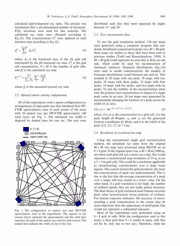
All of the experiments used a sparse configuration (or

arrangement) of open-path rays that simulated four OP-

FTIR spectrometers (one in each corner of the area)

with 10 optical rays per OP-FTIR spectrometer, (40

total rays), see Fig. 1. The simulated ray width is

depicted by dashed lines for one ray. The rays were

F.T.I.R.

retroreflectoropen path ray

Fig. 1. The configuration of optical rays and OP-FTIR

spectrometers used in the experiments. The squares in the

corners (four) represent the spectrometers and the solid lines

represent the path of the optical rays (ten for each source). The

dashed lines indicate the width of one of the rays.

distributed such that they were separated by angles

between 15� and 30�.

2.3. Test concentration data

To test the grid translation method, 120 test maps

were generated using a computer program that ran-

domly distributed concentration peaks on a 40� 40 grid;

these maps are similar to those that have been used in

previous studies (Todd and Ramachandran, 1994). A

40� 40 grid could represent an area that is 40 m on one

side, which could be used for reconstruction of

chemicals outdoors. Gaussian distributions (Eq. (3))

were used to model concentrations; the number of

Gaussian distributions varied between one and six. This

resulted in 20 maps with one peak, 38 maps with two

peaks, 28 maps with three peaks, 18 maps with four

peaks, 14 maps with five peaks, and two maps with six

peaks. To test the stability of the reconstructions when

only the position (not concentration or shape) of a single

peak varies in an area, 36 test maps were generated by

incrementally changing the location of a peak across the

width of an area.

Cðx; yÞ ¼ Ae�ððx�x0Þ2þðy�y0Þ

2Þ=s2

; ð3Þ

where, C(x,y) is the concentration in a grid cell, A is the

peak height (0–40 ppm, x0 and y0 are the generated

location coordinates (0–40m), and s is the width of the

peak (2.8, 4.2, 5.7 or 7.1m).

2.4. Resolution of reconstruction map

Using the conventional single grid reconstruction

method, the simulated ray sums from the original

40� 40 test map were processed using MLEM on an

8� 8 grid. If the original space was a 40� 40m (1600 sq.

m) where each grid cell was a meter on a side, this would

represent a reconstructed map resolution of 25 sq. m (or

a 5� 5 m grid cell). This could be a resolution applicable

to reconstructing concentrations over a large waste

lagoon. The coarser (lower) the grid resolution, the more

the concentrations of peaks are underestimated. This is

due to the fact that the average concentration of a peak

over a larger cell area results in a lower value. On the

other hand, if a grid resolution is too high, the number

of artifacts (peaks that are not really peaks) increases.

The final choice of grid resolution must balance accurate

peak value reconstruction versus presence of artifacts.

For human exposure estimates, the accuracy of recon-

structing a peak concentration at the source may be

more important than the appearance of small peaks that

would not represent a substantial exposure.

Most of the experiments were performed using an

8� 8 grid of cells. With the configuration used in this

study, a finer grid than 8� 8 results in many cells that

are hit by only one or two rays. Therefore, while the

ARTICLE IN PRESSW. Verkruysse, L.A. Todd / Atmospheric Environment 38 (2004) 1801–18091804

number of knowns (ray sums) are constant, the number

of unknowns (individual cell concentration values)

increases with a higher resolution. To investigate the

impact of the reconstruction grid cell resolution on each

method, a number of reconstructions were performed

using resolutions of 7� 7 and 9� 9 grid cells as well.

2.5. Grid translation method

One important limitation in the conventional method

of choosing a fixed single reconstruction grid is that the

location of the edges of the grid cells in relation to a

peak position and shape can adversely impact recon-

struction accuracy. For example, if a peak in the original

high-resolution map is distributed across multiple grid

cells, the highest value that is reconstructed in these cells

can severely underestimate the actual peak value.

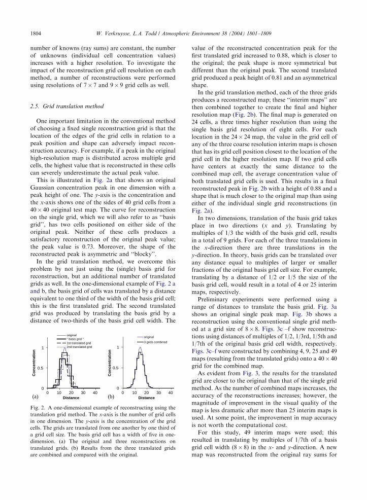
This is illustrated in Fig. 2a that shows an original

Gaussian concentration peak in one dimension with a

peak height of one. The y-axis is the concentration and

the x-axis shows one of the sides of 40 grid cells from a

40� 40 original test map. The curve for reconstruction

on the single grid, which we will also refer to as ‘‘basis

grid’’, has two cells positioned on either side of the

original peak. Neither of these cells produces a

satisfactory reconstruction of the original peak value;

the peak value is 0.73. Moreover, the shape of the

reconstructed peak is asymmetric and ‘‘blocky’’.

In the grid translation method, we overcome this

problem by not just using the (single) basis grid for

reconstruction, but an additional number of translated

grids as well. In the one-dimensional example of Fig. 2 a

and b, the basis grid of cells was translated by a distance

equivalent to one third of the width of the basis grid cell;

this is the first translated grid. The second translated

grid was produced by translating the basis grid by a

distance of two-thirds of the basis grid cell width. The

0

0.5

Co

nce

ntr

atio

n

Co

nce

ntr

atio

n

1

0 10 20 30 40Distance

original" basis grid "1st translated grid2nd translated grid

(a) (b)

0

0.5

1

0 10 20 30 40Distance

original

3 grids combined

Fig. 2. A one-dimensional example of reconstructing using the

translation grid method. The x-axis is the number of grid cells

in one dimension. The y-axis is the concentration of the grid

cells. The grids are translated from one another by one third of

a grid cell size. The basis grid cell has a width of five in one-

dimension. (a) The original and three reconstructions on

translated grids. (b) Results from the three translated grids

are combined and compared with the original.

value of the reconstructed concentration peak for the

first translated grid increased to 0.88, which is closer to

the original; the peak shape is more symmetrical but

different than the original peak. The second translated

grid produced a peak height of 0.81 and an asymmetrical

shape.

In the grid translation method, each of the three grids

produces a reconstructed map; these ‘‘interim maps’’ are

then combined together to create the final and higher

resolution map (Fig. 2b). The final map is generated on

24 cells, a three times higher resolution than using the

single basis grid resolution of eight cells. For each

location in the 24� 24 map, the value in the grid cell of

any of the three coarse resolution interim maps is chosen

that has its grid cell position closest to the location of the

grid cell in the higher resolution map. If two grid cells

have centers at exactly the same distance to the

combined map cell, the average concentration value of

both translated grid cells is used. This results in a final

reconstructed peak in Fig. 2b with a height of 0.88 and a

shape that is much closer to the original map than using

either of the individual single grid reconstructions (in

Fig. 2a).

In two dimensions, translation of the basis grid takes

place in two directions (x and y). Translating by

multiples of 1/3 the width of the basis grid cell, results

in a total of 9 grids. For each of the three translations in

the x-direction there are three translations in the

y-direction. In theory, basis grids can be translated over

any distance equal to multiples of larger or smaller

fractions of the original basis grid cell size. For example,

translating by a distance of 1/2 or 1/5 the size of the

basis grid cell, would result in a total of 4 or 25 interim

maps, respectively.

Preliminary experiments were performed using a

range of distances to translate the basis grid. Fig. 3a

shows an original single peak map. Fig. 3b shows a

reconstruction using the conventional single grid meth-

od at a grid size of 8� 8. Figs. 3c –f show reconstruc-

tions using distances of multiples of 1/2, 1/3rd, 1/5th and

1/7th of the original basis grid cell width, respectively.

Figs. 3c–f were constructed by combining 4, 9, 25 and 49

maps (resulting from the translated grids) onto a 40� 40

grid for the combined map.

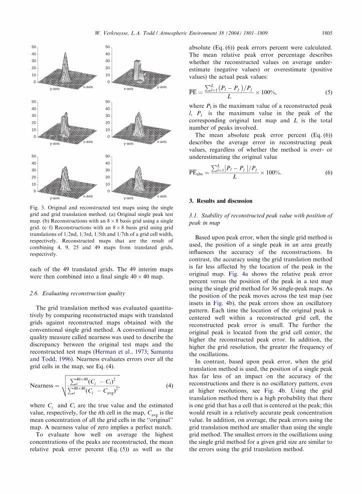
As evident from Fig. 3, the results for the translated

grid are closer to the original than that of the single grid

method. As the number of combined maps increases, the

accuracy of the reconstructions increases; however, the

magnitude of improvement in the visual quality of the

map is less dramatic after more than 25 interim maps is

used. At some point, the improvement in map accuracy

is not worth the computational cost.

For this study, 49 interim maps were used; this

resulted in translating by multiples of 1/7th of a basis

grid cell width (8� 8) in the x- and y-direction. A new

map was reconstructed from the original ray sums for

ARTICLE IN PRESS

0

10

20

30

40

50

x-axisy-axis

0

10

20

30

40

50

y-axisx-axis

0

10

20

30

40

50

x-axisy-axis

0

10

20

30

40

50

x-axisy-axis

0

10

20

30

40

50

x-axisy-axis

0

10

20

30

40

50

x-axisy-axis

Fig. 3. Original and reconstructed test maps using the single

grid and grid translation method. (a) Original single peak test

map. (b) Reconstructions with an 8� 8 basis grid using a single

grid. (c–f) Reconstructions with an 8� 8 basis grid using grid

translations of 1/2nd, 1/3rd, 1/5th and 1/7th of a grid cell width,

respectively. Reconstructed maps that are the result of

combining 4, 9, 25 and 49 maps from translated grids,

respectively.

W. Verkruysse, L.A. Todd / Atmospheric Environment 38 (2004) 1801–1809 1805

each of the 49 translated grids. The 49 interim maps

were then combined into a final single 40� 40 map.

2.6. Evaluating reconstruction quality

The grid translation method was evaluated quantita-

tively by comparing reconstructed maps with translated

grids against reconstructed maps obtained with the

conventional single grid method. A conventional image

quality measure called nearness was used to describe the

discrepancy between the original test maps and the

reconstructed test maps (Herman et al., 1973; Samanta

and Todd, 1996). Nearness evaluates errors over all the

grid cells in the map, see Eq. (4).

Nearness ¼

ffiffiffiffiffiffiffiffiffiffiffiffiffiffiffiffiffiffiffiffiffiffiffiffiffiffiffiffiffiffiffiffiffiffiffiffiffiffiffiffiffiffiffiP40�40i ðC�

i � CiÞ2

P40�40i ðC�

i � C�avgÞ

2;

vuut ð4Þ

where C�i and Ci are the true value and the estimated

value, respectively, for the ith cell in the map, C�avg is the

mean concentration of all the grid cells in the ‘‘original’’

map. A nearness value of zero implies a perfect match.

To evaluate how well on average the highest

concentrations of the peaks are reconstructed, the mean

relative peak error percent (Eq. (5)) as well as the

absolute (Eq. (6)) peak errors percent were calculated.

The mean relative peak error percentage describes

whether the reconstructed values on average under-

estimate (negative values) or overestimate (positive

values) the actual peak values:

PE ¼

PLl¼1 Pl � P�l

� �=P�l

L� 100%; ð5Þ

where Pl is the maximum value of a reconstructed peak

l, P�l is the maximum value in the peak of the

corresponding original test map and L is the total

number of peaks involved.

The mean absolute peak error percent (Eq. (6))

describes the average error in reconstructing peak

values, regardless of whether the method is over- or

underestimating the original value

PEabs ¼

PLl¼1 Pl � P�l

=P�lL

� 100%: ð6Þ

3. Results and discussion

3.1. Stability of reconstructed peak value with position of

peak in map

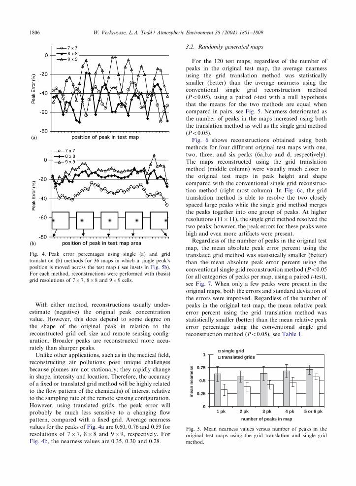
Based upon peak error, when the single grid method is

used, the position of a single peak in an area greatly

influences the accuracy of the reconstructions. In

contrast, the accuracy using the grid translation method

is far less affected by the location of the peak in the

original map. Fig. 4a shows the relative peak error

percent versus the position of the peak in a test map

using the single grid method for 36 single-peak maps. As

the position of the peak moves across the test map (see

insets in Fig. 4b), the peak errors show an oscillatory

pattern. Each time the location of the original peak is

centered well within a reconstructed grid cell, the

reconstructed peak error is small. The further the

original peak is located from the grid cell center, the

higher the reconstructed peak error. In addition, the

higher the grid resolution, the greater the frequency of

the oscillations.

In contrast, based upon peak error, when the grid

translation method is used, the position of a single peak

has far less of an impact on the accuracy of the

reconstructions and there is no oscillatory pattern, even

at higher resolutions, see Fig. 4b. Using the grid

translation method there is a high probability that there

is one grid that has a cell that is centered at the peak; this

would result in a relatively accurate peak concentration

value. In addition, on average, the peak errors using the

grid translation method are smaller than using the single

grid method. The smallest errors in the oscillations using

the single grid method for a given grid size are similar to

the errors using the grid translation method.

ARTICLE IN PRESS

Fig. 4. Peak error percentages using single (a) and grid

translation (b) methods for 36 maps in which a single peak’s

position is moved across the test map ( see insets in Fig. 5b).

For each method, reconstructions were performed with (basis)

grid resolutions of 7� 7, 8� 8 and 9� 9 cells.

0

0.25

0.5

0.75

1

1 pk 2 pk 3 pk 4 pk 5 or 6 pk

number of peaks in map

mea

n n

eam

ess

single gridtranslated grids

Fig. 5. Mean nearness values versus number of peaks in the

original test maps using the grid translation and single grid

method.

W. Verkruysse, L.A. Todd / Atmospheric Environment 38 (2004) 1801–18091806

With either method, reconstructions usually under-

estimate (negative) the original peak concentration

value. However, this does depend to some degree on

the shape of the original peak in relation to the

reconstructed grid cell size and remote sensing config-

uration. Broader peaks are reconstructed more accu-

rately than sharper peaks.

Unlike other applications, such as in the medical field,

reconstructing air pollutions pose unique challenges

because plumes are not stationary; they rapidly change

in shape, intensity and location. Therefore, the accuracy

of a fixed or translated grid method will be highly related

to the flow pattern of the chemical(s) of interest relative

to the sampling rate of the remote sensing configuration.

However, using translated grids, the peak error will

probably be much less sensitive to a changing flow

pattern, compared with a fixed grid. Average nearness

values for the peaks of Fig. 4a are 0.60, 0.76 and 0.59 for

resolutions of 7� 7, 8� 8 and 9� 9, respectively. For

Fig. 4b, the nearness values are 0.35, 0.30 and 0.28.

3.2. Randomly generated maps

For the 120 test maps, regardless of the number of

peaks in the original test map, the average nearness

using the grid translation method was statistically

smaller (better) than the average nearness using the

conventional single grid reconstruction method

(Po0.05), using a paired t-test with a null hypothesis

that the means for the two methods are equal when

compared in pairs, see Fig. 5. Nearness deteriorated as

the number of peaks in the maps increased using both

the translation method as well as the single grid method

(Po0.05).

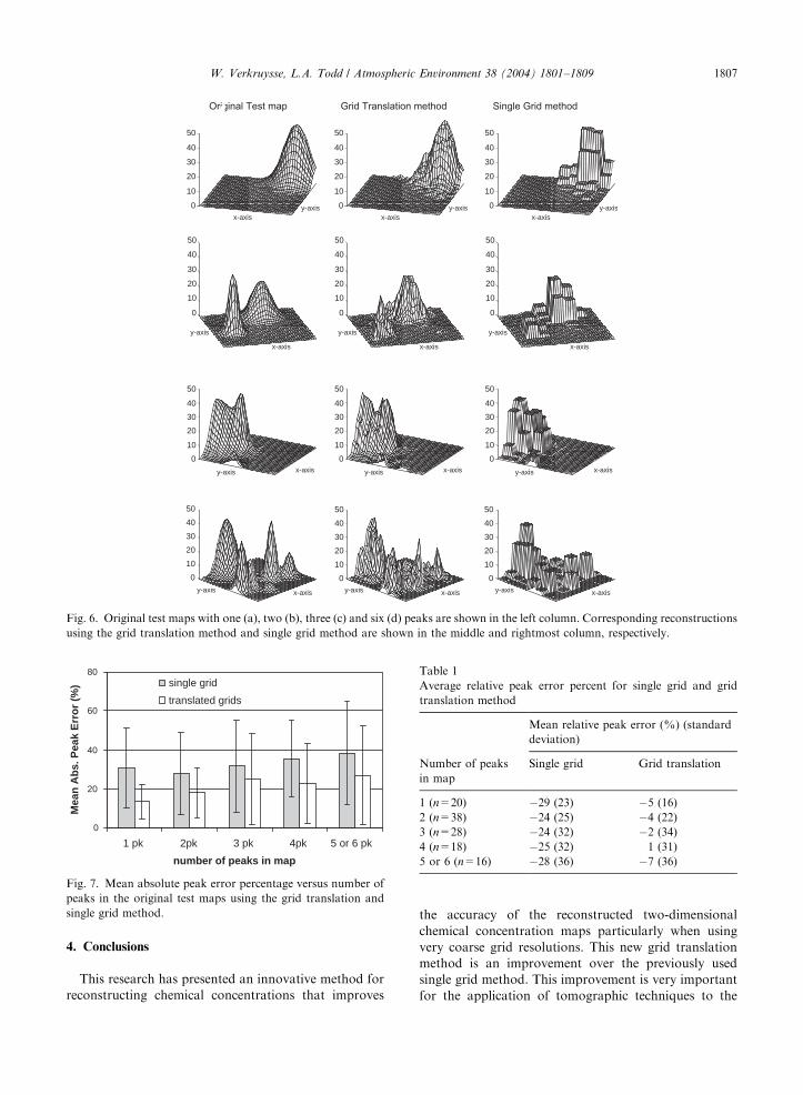
Fig. 6 shows reconstructions obtained using both

methods for four different original test maps with one,

two, three, and six peaks (6a,b,c and d, respectively).

The maps reconstructed using the grid translation

method (middle column) were visually much closer to

the original test maps in peak height and shape

compared with the conventional single grid reconstruc-

tion method (right most column). In Fig. 6c, the grid

translation method is able to resolve the two closely

spaced large peaks while the single grid method merges

the peaks together into one group of peaks. At higher

resolutions (11� 11), the single grid method resolved the

two peaks; however, the peak errors for these peaks were

high and even more artifacts were present.

Regardless of the number of peaks in the original test

map, the mean absolute peak error percent using the

translated grid method was statistically smaller (better)

than the mean absolute peak error percent using the

conventional single grid reconstruction method (Po0.05

for all categories of peaks per map, using a paired t-test),

see Fig. 7. When only a few peaks were present in the

original maps, both the errors and standard deviation of

the errors were improved. Regardless of the number of

peaks in the original test map, the mean relative peak

error percent using the grid translation method was

statistically smaller (better) than the mean relative peak

error percentage using the conventional single grid

reconstruction method (Po0.05), see Table 1.

ARTICLE IN PRESS

Original Test map

0

10

20

30

40

50

x-axisy-axis

0

10

20

30

40

50

x-axisy-axis

0

10

20

30

40

50

x-axis

y-axis

0

10

20

30

40

50

y-axisx-axis

0

10

20

30

40

50

x-axisy-axis

0

10

20

30

40

50

x-axisy-axis

0

10

20

30

40

50

x-axis

y-axis

0

10

20

30

40

50

y-axisx-axis

0

10

20

30

40

50

x-axisy-axis

0

10

20

30

40

50

x-axisy-axis

0

10

20

30

40

50

x-axis

y-axis

0

10

20

30

40

50

y-axisx-axis

Grid Translation method Single Grid method

Fig. 6. Original test maps with one (a), two (b), three (c) and six (d) peaks are shown in the left column. Corresponding reconstructions

using the grid translation method and single grid method are shown in the middle and rightmost column, respectively.

0

20

40

60

80

1 pk 2pk 3 pk 4pk 5 or 6 pk

number of peaks in map

Mea

n A

bs.

Pea

k E

rro

r (%

) single grid

translated grids

Fig. 7. Mean absolute peak error percentage versus number of

peaks in the original test maps using the grid translation and

single grid method.

Table 1

Average relative peak error percent for single grid and grid

translation method

Mean relative peak error (%) (standard

deviation)

Number of peaks

in map

Single grid Grid translation

1 (n=20) �29 (23) �5 (16)

2 (n=38) �24 (25) �4 (22)

3 (n=28) �24 (32) �2 (34)

4 (n=18) �25 (32) 1 (31)

5 or 6 (n=16) �28 (36) �7 (36)

W. Verkruysse, L.A. Todd / Atmospheric Environment 38 (2004) 1801–1809 1807

4. Conclusions

This research has presented an innovative method for

reconstructing chemical concentrations that improves

the accuracy of the reconstructed two-dimensional

chemical concentration maps particularly when using

very coarse grid resolutions. This new grid translation

method is an improvement over the previously used

single grid method. This improvement is very important

for the application of tomographic techniques to the

ARTICLE IN PRESSW. Verkruysse, L.A. Todd / Atmospheric Environment 38 (2004) 1801–18091808

environmental field where the number of instruments

(and, therefore, number of measurements) is limited and

the chemical plumes that are reconstructed are always

changing in concentration magnitude and spatial loca-

tion.

Using the grid translation method, the nearness and

concentration peak error percentages were considerably

smaller than when using the single grid method.

Absolute peak error percents were reduced by as much

as 40% and relative peak errors were reduced well over

four times using the grid translation method. The

importance of the nearness statistic is that it represents

errors in reconstruction of the peak shape, concentra-

tion, and location, as well as the appearance of artifacts.

This improvement in peak concentration errors would

potentially impact the accuracy of evaluating human

exposures in the industrial hygiene field and of calculat-

ing chemical emissions in the environmental field.

The improvement obtained using this grid translation

method is important for several reasons. First, it reduces

the significance of choosing a single optimum grid

resolution for a given application. In practice, the choice

of grid resolution is limited by the configuration

(number and position of rays) of the remote sensing

equipment. Up to a point, as the grid resolution is

increased, the reconstruction of peak concentration

values improves with both methods. However, when a

grid resolution becomes too fine with respect to the

number of rays, it is possible for only two, one, or no

rays to hit a grid cell; this is likely to result in a

reconstructed map with pronounced artifacts. With the

single grid method, as these higher grid resolutions are

selected, peak concentration errors unpredictably in-

crease or decrease. With the grid translation method,

while the peak errors change with the selection of

different basis grid resolutions, on average, the change

in errors are small and the errors tend to decrease with

higher grid resolutions.

The second significant improvement comes from the

stability of the grid translation method compared to the

single grid cell method, in regards to the location of a

peak in a space. For a given optical remote sensing

configuration, using the grid translation method, the

location of a single peak within a map had little impact

on the accuracy of the reconstruction. This is very

important because chemical plumes are always in flux

and the concentration distribution changes over time

and space. Therefore, regardless of the reconstruction

method used for mapping concentrations of chemicals in

air, the accuracy of the reconstructed peak shape, peak

concentration and number of peaks, can be adversely

impacted using a conventional fixed single grid method.

The grid translation method can use the same basis

grid size as the single grid method, and produce

reconstructions that resolve features that are missing

using the single grid method. When a single grid is used

for a reconstruction, the resulting map is obviously of

the same resolution as the selected grid size; this is

generally coarser than desired. As the resolution of the

reconstruction grid is increased, there is a risk of

producing more artifacts in the reconstruction. The

image resolution of a single grid reconstructed map can

be increased by first adding synthetic rays in between the

actual rays using interpolation techniques and then

creating a higher resolution map. Alternatively, grid

cells can be added to the coarser maps using interpola-

tion techniques. Either way, these techniques require

assumptions to be made about the underlying chemical

distribution. The proposed grid translation method

allows for an effectively higher resolution than the

resolution of the basis grid (and single grid method)

without requiring prior assumptions regarding the

concentration distribution and without risking the

increased presence of artifacts.

Finally, peak concentration errors are smaller using

the new method compared with the conventional

method because the use of multiple grids increases the

likelihood that there is at least one cell that closely

matches the position of a peak and thus gives a relatively

accurate peak value reconstruction.

This research provides a significant improvement over

conventional methods for reconstructing chemical plumes

in air using an environmental CAT scanning system. In

particular, this improvement is important for coarse

resolutions. Given the sparse remote sensing configura-

tions that must be used in the environmental and

industrial hygiene applications of this method, the ability

to produce high-resolution maps with few measurements

is significant. This improvement was achieved without

artificially interpolating additional optical rays and with-

out using any assumptions about the underlying resolu-

tion or the number of peaks in the map. Further

optimization of parameters such as number of iterations

and type of configurations may improve the presented

method even more. This work is underway.

Acknowledgements

This material is based upon work supported by the

National Science Foundation under Grant Number

00011385. We would like to thank Rob Katz for his

technical assistance with programming the algorithms

and Dr. Kathleen Mottus with technical support with

the manuscript.

References

Byer, R.L., Shepp, L.A., 1979. Two-dimensional remote air

pollution via tomography. Applied Optics Letters 4 (3),

75–79.

ARTICLE IN PRESSW. Verkruysse, L.A. Todd / Atmospheric Environment 38 (2004) 1801–1809 1809

Cormack, A.M., 1964. Representation of a function by its line

integrals, with some radiological applications II. Journal of

Applied Physics 35, 2908–2913.

Drescher, A.C., Gadgil, A.J., Price, P.N., Nazaroff, W.W.,

1996. Novel approach for tomographic reconstruction of

gas concentration distributions in air: use of smooth basis

functions and simulated annealing. Atmospheric Environ-

ment 36 (6), 929–940.

Herman, G.T., Lent, A., Rowland, S.W., 1973. Art: mathematics

and applications. A report on the mathematical foundations

and on the applicability to real data of the algebraic recon-

struction techniques. Journal of Theoretical Biology 42, 1–32.

Hounsfield, G.N., 1973. Computerized transverse axial scan-

ning (tomography): Part 1. Description of a system. British

Journal of Radiology 46, 1016–1022.

Samanta, A., Todd, L.A., 1996. Mapping air contaminants

indoors using a prototype computed tomography system.

Annals of Occupational Hygiene 40 (6), 675–691.

Samanta, A., Todd, L.A., 2000. Mapping chemicals in air using

an environmental cat scanning system: evaluation of

algorithms. Atmospheric Environment 34, 699–709.

Shepp, L.A., Vardi, Y., 1982. Maximum likelihood reconstruc-

tion for emission tomography. IEEE Transactions on

Medical Imaging MI-1 (2), 113–122.

Todd, L.A., Leith, D., 1990. Remote sensing and computed

tomography in industrial hygiene. American Industrial

Hygiene Association Journal 51, 224–233.

Todd, L.A., Ramachandran, G., 1994. Evaluation of algo-

rithms for tomographic reconstruction of chemical

concentrations in indoor air. American Industrial Hygiene

Association Journal 55 (5), 403–417.

Todd, L.A., Ramanathan, M., Mottus, K., Katz, R., Dodson,

A., Mihlan, G., 2001. Measuring chemical emissions using

open-path fourier transform infrared (OP-FTIR) spectro-

scopy and computer assisted tomography. Atmospheric

Environment 35, 1937–1947.

Tsui, B.M.W., Zhao, X.D., Frey, E.C., Gulberg, G.T., 1991.

Comparison between ML-EM and WLS-CG algorithms for

spect image-reconstruction. IEEE Transactions on Nuclear

Science 38 (6), 1766–1772.

Yost, M.G., Gadgil, A.J., Drescher, A.C., Zhou, Y., Simonds,

M.A., Levine, S.P., Nazaroff, W.W., Saison, P.A., 1994.

Imaging indoor tracer-gas concentrations with computed

tomography: experimental results with a remote sensing

FTIR system. American Industrial Hygiene Association

Journal 55 (5), 395–402.

Warland, J.S., Dias, G.M., Thurtell, G.W., 2001. A tunable

diode laser system for ammonia flux measurements

over multiple plots. Environmental Pollution 114 (2),

215–221.

Wolfe, D.C., Byer, R.L., 1979. Model studies of laser

absorption computed tomography for remote air pollution

measurement. Applied Optics 21, 1165–1177.