AIAA 95-1740

1

Implicit/Multigrid Algorithms for Incompressible TurbulentFlows on Unstructured Grids

W. Kyle Anderson,* Russ D. Rausch,† Daryl L. Bonhaus‡NASA Langley Research Center, Hampton, Virginia 23681

Summary

An implicit code for computing inviscid and viscous incompressible flows on unstructured grids is described. The foundation of thecode is a backward Euler time discretization for which the linear system is approximately solved at each time step with either a pointimplicit method or a preconditioned Generalized Minimal Residual (GMRES) technique. For the GMRES calculations, several tech-niques are investigated for forming the matrix-vector product. Convergence acceleration is achieved through a multigrid scheme thatuses non-nested coarse grids that are generated using a technique described in the present paper. Convergence characteristics areinvestigated and results are compared with an exact solution for the inviscid flow over a four-element airfoil. Viscous results, whichare compared with experimental data, include the turbulent flow over a NACA 4412 airfoil, a three-element airfoil for which Machnumber effects are investigated, and three-dimensional flow over a wing with a partial-span flap.

*Senior Research Scientist, Aerodynamic and Acoustic MethodsBranch, Fluid Mechanics and Acoustics Division, Member AIAA.

†Research performed while a Resident Research Associate,National Research Council. Currently Senior Engineer, LockheedEngineering and Sciences Company, Member AIAA.

‡Research Scientist, Aerodynamic and Acoustic MethodsBranch, Fluid Mechanics and Acoustics Division, Member AIAA

Copyright © 1995 by the American Institute of Aeronautics andAstronautics, Inc. No copyright is asserted in the United Statesunder Title 17, U.S. Code. The U.S. Government has a royalty-freelicense to exercise all rights under the copyright claimed herein forGovernmental purposes. All other rights are reserved by the copy-right owner.

IntroductionIn the past decade, much progress has been made in devel-

oping computational techniques for predicting flow fieldsabout complex configurations. These techniques include bothstructured- and unstructured-grid algorithms. The accuracyand efficiency of these codes is now such that computationalfluid dynamics (CFD) is routinely used in the analysis andimprovement process of existing designs and is a valuabletool in experimental programs and in the design of new con-figurations.

Many existing codes referred to above have been devel-oped in support of the aircraft industry and, therefore, solvethe compressible flow equations because of the need to han-dle the important effects associated with transonic Machnumbers. However, many important problems, such as thosein the automobile industry and in biomechanics, are inher-ently incompressible and must be treated appropriately.

With the success and wide availability in recent years ofthe compressible codes, these codes have naturally been con-sidered for use with incompressible flows by simply loweringthe Mach number to minimize compressibility effects. Unfor-tunately, as the Mach number is successively decreased to-ward zero, the performance of the compressible codes interms of both convergence rate and accuracy suffers greatly.In Ref.52, Volpe demonstrated the poor performance of com-pressible flow codes under these conditions, particularly forMach numbers below approximately 0.1.

To overcome the difficulties associated with use of com-pressible codes, excellent progress has been made in the useof local preconditioners to extend the applicability of thesecodes to low Mach numbers. Several examples of this tech-nique, as well as the necessary theory, can be found inRefs. 13, 18, 24, 47, 48, 49, and54. Preconditioning is indeeda viable means of extending the applicability of compressible

flow codes to the low-Mach-number range and continues tobe an area of active research. A computer code that utilizesthis technique has the added benefit of being able to handleboth compressible and incompressible flows. This techniquehas been applied to both steady-state and time-dependentflows; for time-dependent flows, however, a subiterative pro-cess is required to maintain time accuracy.

Another available method of extending a compressibleflow code for use at zero Mach number is the method of arti-ficial compressibility first introduced by Chorin.14 In this ap-proach, a pseudo-time derivative of pressure is added to thecontinuity equation, which allows the continuity equation tobe advanced in a time-marching manner, much the same asthe momentum equations. Artificial compressibility has beensuccessfully applied by several researchers for both steady-state and time-dependent flows (e.g., Refs. 12, 21, 32, 35, 36,43, and44). When the temperature field is not required, thistechnique offers an advantage over preconditioning methodsin that the energy equation is not solved; therefore, the effi-ciency of the algorithm is enhanced both in terms of computertime and reduced memory. The reduction in memory is par-ticularly significant for implicit codes on unstructured gridsbecause the storage associated with the time linearization ofthe fluxes is reduced by the square of the local block size, orroughly 40 percent. As with preconditioning, the use of thismethod for time-dependent flows requires a subiterative pro-cedure to obtain a divergence-free velocity field at each timestep.

Recently, unstructured grids have been explored for CFDproblems (e.g., Refs.1, 5, 6, 10,26, and 28). This approachhas several advantages over structured grids for problems thatinvolve complex geometries and flows. The biggest advan-tage is the reduction in time needed to generate grids within acomplex computational domain. Another advantage is thatunstructured grids lend themselves to adaptive-grid methodsbecause new nodes can be added to a localized region of themesh by modifying a small subset of the overall grid datastructure. Although the unstructured-grid approach enjoysthese advantages over structured grids, flow solvers that uti-lize it suffer from several disadvantages. These primarily in-clude a factor of 2-3 increase in memory requirements andcomputer run times on a per grid point basis.

The purpose of the current work is to extend the unstruc-tured-grid compressible flow code described in Refs.1, 2,and 10 to incompressible flows. The extension provides acode that can be used in the design of airplanes, ships, auto-mobiles, pumps, ducts, and turbomachinery. The extensionalso provides a tool for studying Mach-number effects on

2

high-lift airfoils because of the existence of both incompress-ible and compressible flow codes with similar levels of nu-merical accuracy that can be run on identical grids. The cur-rent code is a node-based upwind implicit code that usesmultigrid acceleration (in two dimensions) to reduce the com-puter time required for steady-state computations. In this ex-tension, the artificial compressibility approach is used. Thechoice of this technique over preconditioning is based prima-rily on the desire to reduce memory requirements and com-puter time by reducing the number of equations.

In the remainder of the paper, the governing equations aregiven, and the basic solution algorithm is described. Althoughboth two- and three-dimensional results are shown in the pa-per, the description of the equations, algorithms, and bound-ary conditions are limited to two-dimensional flow to con-serve space. Results are presented to demonstrate theincompressible code. Inviscid flow results for a four-elementairfoil are compared with an exact solution and are used forexamining the effects of various parameters on the conver-gence behavior. Viscous, turbulent flow results for the NACA4412 airfoil are compared with experimental data, as well aswith results from a well-known structured-grid compressiblecode run at a low Mach number. In addition, results are pre-sented for a three-element airfoil to study the effects of com-pressibility. These results are compared with results from anunstructured-grid compressible code and with experimentaldata. Finally, three-dimensional turbulent computations areshown for a wing with a partial-span flap.

Governing EquationsThe governing equations are the incompressible Navier-

Stokes equations augmented with artificial compressibility.These equations represent a system of conservation laws for acontrol volume that relates the rate of change of a vector ofaverage state variables to the flux through the volume sur-face. The equations are written in integral form as

(1)

where is the outward-pointing unit normal to the controlvolume . The vector of dependent state variables and theinviscid and viscous fluxes normal to the control volumeand are given as

(2)

(3)

(4)

where is the artificial compressibility parameter; andare the Cartesian velocity components in the and direc-tions, respectively; is the velocity normal to the surface ofthe control volume, where

(5)

and is the pressure. The shear stresses in Eq.(4) are givenas

(6)

where and are the laminar and turbulent viscosities, re-spectively, and is the Reynolds number.

Solution AlgorithmThe baseline flow solver is an implicit upwind algorithm in

which the inviscid fluxes are obtained on the faces of eachcontrol volume with a flux-difference-splitting scheme. Forthe current algorithm, a node-based scheme is used in whichthe variables are stored at the vertices of the grid and theequations are solved on nonoverlapping control volumes thatsurround each node. The viscous terms are evaluated with afinite-volume formulation that is equivalent to a Galerkin typeof approximation for these terms. The solution at each timestep is updated with the linearized backward Euler time-dif-ferencing scheme. At each time step, the linear system ofequations is approximately solved with either a point implicitprocedure or the Generalized Minimal Residual (GMRES)method. Details of the flux-difference-splitting scheme andthe time-advancement scheme are given below.

Finite-Volume SchemeThe solution is obtained by dividing the domain into a fi-

nite number of triangles from which non-overlapping controlvolumes are formed by the “dual” mesh described in Refs.1and 5. The inviscid fluxes are evaluated on the faces of thecontrol volumes with a flux-difference-splitting scheme simi-lar to that used in Refs. 21, 32, 35, and 43.

The inviscid fluxes on the boundaries of the control vol-umes are given by

(7)

where is the numerical flux, is the flux vector given inEq. (3), and are the values of the dependent variableson the left and right side of the boundary of the control vol-ume, and

(8)

where is a diagonal matrix whose elements are the eigen-values of the flux Jacobian, , and are given by

(9)

and

(10)

The matrices of right and left eigenvectors are given by

q

Vt∂

∂qf i n⋅

Ω∂∫° ld f v n⋅ ld

Ω∂∫°–+ 0=

nV q

f if v

qp

u

v

=

f i n⋅βΘ

uΘ nxp+

vΘ nyp+

=

f v n⋅0

nxτxx nyτxy+

nxτxy nyτyy+

=

β u vx y

Θ

Θ nxu nyv+=

p

τxx µ µt+( ) 2Re------ux=

τyy µ µt+( ) 2Re------vy=

τxy µ µt+( ) 1Re------ uy vx+( )=

µ µtRe

Φ 12--- f q+ n;( ) f q- n;( )+( ) 1

2--- A q+ q-–( )–=

Φ fq+ q-

A T Λ T1–

=

ΛA

λ1 Θ=

λ2 Θ c+=

λ3 Θ c–=

c Θ2 β+=

3

(11)

(12)

where is a shear velocity perpendicular to and equal to

(13)

In Eqs.(7)-(12), the ~ represents quantities evaluated with av-eraged values of the left and right states. The values of the leftand right states and are evaluated with a Taylor seriesexpansion about the central node of the control volume, sothat the data on the face is given by

(14)

where is the vector that extends from the central node to themidpoint of each edge and is the gradient of the depen-dent variables at the node and is evaluated with a least-squares procedure.1,3,7

Since the right and left eigenvectors given in Eqs.(11) and(12) contain the variable (and therefore ), the steady-statesolution has a dependency on, where larger values corre-spond to increased dissipation.32 Numerical experiments haveindicated that this influence is small for values of belowapproximately 100. Also, since large values of correspondto large values of , if is chosen to be very large, there is awide disparity in the magnitudes of the eigenvalues. This dis-parity could lead to slow convergence rates in much the samemanner as when a compressible flow solver is used at verylow freestream Mach numbers. For these reasons, all the re-sults obtained in this paper use a of 10.

Time-Advancement SchemeThe time-advancement algorithm is based on the linearized

backward Euler time-differencing scheme, which yields a lin-ear system of equations for the solution at each time step:

(15)

where is the vector of steady-state residuals,represents the change in the dependent variables, and

(16)

The solution of this system of equations is obtained with ei-ther a fully vectorizable point implicit Gauss-Seidelprocedure1,3 or a preconditioned GMRES procedure.37

When using the Gauss-Seidel procedure, the solution of thelinear system is obtained by a relaxation scheme in which

is obtained through a sequence of iteratesthat converge to . To clarify the scheme, is firstwritten as a linear combination of two matrices that representthe diagonal and off-diagonal terms:

(17)

The simplest iterative scheme for obtaining a solution tothe linear system of equations is a Jacobi type of method inwhich all off-diagonal terms (i.e., ) are taken tothe right-hand side of equation (15) and are evaluated with thevalues of from the previous subiteration level . Thisscheme can be represented as

(18)

The convergence rate of this process can be slow but can beaccelerated somewhat by using the latest values of assoon as they are available. This can be achieved by adopting aGauss-Seidel type of strategy in which all odd-numberednodes are updated first, followed by the solution of the even-numbered nodes. This procedure can be represented as

(19)

where is the most recent value of , whichwill be at subiteration level for the odd-numbered nodesthat have been previously updated and at level for the even-numbered nodes.

Although the use of this algorithm offers improvement overthe Jacobi iteration strategy, the convergence of the linearsystem can still be slow, particularly on fine grids. Fortu-nately, full convergence of the linear system is not necessaryto provide a robust algorithm that remains stable at time stepsmuch larger than an explicit scheme. In fact, if the residual isnot linearized accurately, then solving the linear system be-yond truncation error of the non-linear equation is a waste ofresources because the Newton type of convergence that isnormally obtained as the time step is increased is lost. Numer-ical experiments over a wide range of test cases for both vis-cous and inviscid flow indicate that 15–20 subiterations ateach time step is adequate. The memory requirements for thisscheme are dominated by the storage of the flux Jacobians as-sociated with the linearization of the fluxes on each edge. Inthe present implementation, two matrices are stored on eachedge and are associated with the linearization of the flux withthe states on the right and left sides of the face. In two dimen-sions, each matrix is so that a total of 18 storage loca-tions are required for each edge. In three dimensions, the ma-trices are each so that 32 storage locations are requiredfor every edge in the mesh. In equation (19), the multiplica-tion of the off-diagonal terms in the matrix by the correspond-ing values of is computed by looping over the edgesin the mesh and multiplying the flux Jacobians by the currentvalues of . Note that when the Gauss-Seidel scheme isused as described above, only the dependency of the flux onthe nodes that lie at each end of an edge are included; thus, thelinearization of the second-order residual is only approximateand would only be exact if the flux were computed with afirst-order-accurate scheme. The convergence of the subitera-tive procedure is greatly enhanced by smaller time steps,which results in larger diagonal contributions. Therefore, acompromise must be made to allow Courant-Friedrichs-Lewy(CFL) numbers that are small enough for good convergenceof the linear system but large enough to provide good conver-gence of the nonlinear system. Experiments have shown thatalthough computations with CFL numbers of 500 or more re-main stable, the best convergence in terms of computer timefor the Navier-Stokes equations is achieved for more moder-ate CFL numbers between 100 and 200.

When the Gauss-Seidel scheme is used, practical applica-tion has shown that replacing the exact linearization of the

T QTR0 c Θ c–( )– c Θ c+( )ny– nxc nyφ– nxc nyφ+( )–

nx nyc nxφ+ n– yc nxφ+

= =

T 1– R 1– Q=

φc2----–

φΘnx nyc2+

c2------------------------------–

φ– Θny nyc2+

c2---------------------------------

1

2c2-------- Θ c+( )

2c2------------------nx

Θ c+( )2c2

------------------ny

1

2c2-------- Θ c–( )

2c2-----------------nx

Θ c–( )2c2

-----------------ny

=

φ Θ

φ nxv nyu–=

q+ q-

qface qnode q r⋅∇+=

r∇q

c ββ

ββ

c β

β

A[ ]n ∆q n r n=

r n ∆q

A[ ]n V∆t----- I

q∂∂r+=

∆q n ∆q i

∆q n A[ ]n

A[ ]n D[ ]n O[ ]n+=

O[ ]n ∆q

∆q i i

D[ ]n ∆q i 1+ r n O[ ] ∆q i–[ ]=

∆q

D[ ]n ∆q i 1+ r n O[ ] ∆q i 1+( ) i⁄–[ ]=

∆q i 1+( ) i⁄ q∆i 1+

i

3 3×

4 4×

∆q

∆q

4

fluxes with an approximate linearization can provide a signif-icant increase in robustness, particularly on highly stretchedgrids used for turbulent flow calculations. This increase in ro-bustness is due to the loss of diagonal dominance often asso-ciated with the exact linearizations. For this reason, when theGauss-Seidel scheme is used, the linearizations are based onlinearizing Eq. (7) with treated as constant matrix.

As an alternative to the above procedure, the GMRES37

method can also be used. Note that this procedure only re-quires the formation of the product of with a columnvector and does not require the explicit inversion of .

In the present work, three methods are used to form the ma-trix-vector product required for GMRES. In the first method,the flux Jacobian matrices, stored on each edge, are formedfrom the data that lies at the end point of the edge. This basicprocedure is the same as that described above for the Gauss-Seidel algorithm and is equivalent to an exact linearization ofa spatially first-order-accurate scheme.

The second technique that can be used to form the matrix-vector product is the use of a finite-difference approach4,23,29

(20)

where is the residual evaluated by using per-turbed state quantities. In this study, is a scalar quantitychosen so that the product of with the root mean square(RMS) of is the square root of “machine zero:”

(21)

The choice of is based on keeping the perturbation to thedependent variables in Eq. (20) at a small and consistent levelindependent of the size of the mesh. Note, however, that thevalue of will not necessarily be small but will actually in-crease as the mesh size increases. This relationship can beseen by examining the variation of with increasing meshsize. Because the norm of is always unity, the RMS valueof is determined solely by the inverse of the number of un-knowns in the mesh. In this case, as the mesh size increases, acorresponding decrease occurs in the size of each element of

; as a result, as the mesh size gets larger, a correspondingincrease occurs in the magnitude of. The selection of inthis manner is computationaly efficient and is much more ef-fective than chosing a technique that results in a small valueof . In the latter case, practical application has shown thatthe level of convergence that can be obtained depends greatlyon the size of the mesh and often fails to converge to machinezero.31 This may be attributable to the fact that, because isforced to be small, the size of the perturbation decreases asthe mesh size increases. Eventually, the perturbation is essen-tially zero so that the matrix-vector product that is computedwith Eq. (20) is inaccurate. By computing with Eq.(21),consistent convergence to machine zero is obtained indepen-dent of the mesh size. Note that for the incompressible equa-tions, the values of are reasonably well scaled in that thesize of a typical element of is order one. If the magnitude ofthese variables is substantially different, then a more appro-priate choice of would be to require the product of with atypical size of an element of to be roughly the square rootof machine zero multiplied by a typical size of an element of

.In Eq. (20), if the computation of the residuals is the same

as that used for the right-hand side of Eq.(15), then the result-ing matrix-vector product will match that obtained by usingthe exact linearizations of the second-order system, to withinround off. If the same procedure is used, then the vectorscomputed in the Krylov subspace are essentially equal tothose computed using the full linearization of the higher-order

residuals; however, the need to compute and store the matrixis eliminated.

The final method used to evaluate the matrix-vector prod-uct was introduced recently by Barth8. In this method, the ele-ments of the flux Jacobians are still stored along each edge inthe same manner as when the exact linearization to the first-order scheme is used. However, rather than simply formingthe linearizations from the data at the nearest neighbors, theflux Jacobians are formed from data that are extrapolated tothe cell faces with a least-squares linear reconstruction proce-dure. In addition, the elements of are “reconstructed” withthe same linear reconstruction procedure. Using the methodof Ref. 8, the effect of the exact linearization of the second-order spatial residual is computed by using the same amountof storage that is required for the linearizations of the first-order scheme.

The preconditioning step for the GMRES procedure is donewith one or more iterations of a point Gauss-Seidel procedureor an incomplete lower/upper (LU) decomposition20 in whichno fill in is allowed (i.e., ILU(0)). Note that only one iterationof the Gauss-Seidel procedure is equivalent to “block diago-nal” preconditioning. In all cases, the preconditioning is ap-plied to the left. When GMRES is used with ILU(0) as thepreconditioner, the nonzero terms in the matrix are stored in acompressed-row storage format,17 and the nodes in the meshare reordered with a reverse-Cuthill-McKee algorithm16 tocluster nonzero terms along the diagonal. In addition, the for-ward and back substitution steps, which must be conductedeach time the preconditioner is applied, have been fully vec-torized with a level-scheduling algorithm.38 Vectorization isaccomplished by keeping a list of all edges that contribute tothe nodes in a given level and coloring those edges to allowvectorization. Numerical experiments with the level-schedul-ing algorithm indicate that the computer time required for theforward and backward substitutions is reduced by a factor ofapproximately 3.3 in two dimensions and by a factor of ap-proximately 2.8 in three dimensions. A similar process hasbeen used in Ref. 51.

The memory required for each of the above methods ofsolving the linear system is an important consideration for thepractical usability of the schemes. As already discussed, thelargest demand on memory for the Gauss-Seidel schemecomes from the storage of the Jacobians on each edge. For theGMRES algorithms, the storage can vary significantly, de-pending on what methodology is used for computing the ma-trix-vector product and what type of preconditioning is used.When one or more iterations of the Gauss-Seidel scheme areused for preconditioning, the Jacobians stored along eachedge can be used for both the matrix-vector product and thepreconditioning step. Therefore, this part of the overall stor-age requirement is the same as for the Gauss-Seidel scheme(used alone) in that the Jacobians are essentially stored onlyonce. Note that when ILU(0) is used as a preconditioner, theflux Jacobians that contribute to the global matrix(which is subsequently decomposed into approximate lowerand upper triangular matrices) are formed with the same stor-age requirements as required with only nearest neighbors. Inthis way, even when the matrix-vector product matches thatobtained by linearizing the second-order spatial discretiza-tion, the preconditioner corresponds to a lower order linear-ization. With the exception of the finite-difference technique,the use of ILU(0) preconditioning requires that the elementsof the matrix be stored essentially twice; once to compute thematrix-vector product and once for the incomplete LU de-composition. Additional storage is required to store the vec-tors in the Krylov subspace and is given by the dimension ofthe subspace times the total number of unknowns in the mesh.Although this storage can be nontrivial with a large Krylovsubspace, it is typically approximately one-third of that re-quired for the storage of the nonzero matrix elements.

A

A[ ]ν j A[ ]

Aν j

r q εν j+( ) r q( )–ε

------------------------------------------≈

r q εν j+( )ε

εν j

ε mz ν j RMS⁄=

ε

ε

εν j

ν j

ν jε ε

ε

ε

ε

qq

ε εν j

q

ν j

A[ ]

5

Boundary ConditionsThe boundary conditions on the wall correspond to tan-

gency conditions for inviscid flows and to no-slip conditionsfor viscous flows. In the far field, a locally one-dimensionalcharacteristic type of boundary condition is used, similar tothat described in Refs.32 and 44. By considering the linear-ized inviscid one-dimensional equations (wherex is assumedto be the coordinate normal to the boundary),

(22)

where

Equation (22) can be diagonalized using a similarity transfor-mation to yield a decoupled system of equations

(23)

where represents a vector of characteristic variables

. (24)

The second eigenvalue is always positive and if it isassumed that the normal to the far-field boundary points out-ward, is the same on the boundary as in the interior of themesh. In a similar manner, is always negative; there-fore, is the same on the boundary as in the free stream.The relationship between the value of on the boundary de-pends on whether or not the flow is into or out of the domain;for inflow, the value on the boundary is the same as in the freestream; for outflow it is the same on the boundary as in the in-terior. These relationships provide three equations in three un-knowns that can be solved for the pressure, the normal veloc-ity, and the tangential velocity on the far-field boundary:

(25)

where the subscriptr on the right-hand side of Eq. (25) refersto data taken from outside the domain for inflow and from in-side the domain for outflow. Also, the subscripti indicatesdata taken from inside the domain, and indicates datataken from outside the domain, which includes a point-vortexcorrection to account for lift.45 In the current study, note thatthe values taken as reference conditions (those taken as con-stant in obtaining Eq.(25)) are evaluated at free-stream condi-tions to facilitate the linearization of the fluxes on the far-fieldboundary.

For all boundary nodes, both on the solid boundaries and inthe far field, the boundary conditions are not explicitly set butare obtained through the solution process in the same manneras the points interior to the domain. The only distinction be-tween boundary nodes and an interior node is that the enforce-ment of the boundary condition is reflected in the flux calcu-lation on the boundary and the appropriate linearization istaken into account on the left-hand side of Eq. (16). In thisway, a fully implicit treatment of the boundary conditions isachieved.

Convergence Acceleration TechniquesTo accelerate the convergence to a steady state, a multigrid

algorithm is employed.10 The algorithm is similar to that inRef.28 in that a full approximation scheme11 is employed, thecoarser grids are not directly obtained from to the finest one,and both V and W cycles can be used. The primary differencebetween the present implementation and that of Ref.28 is atthe boundaries for the interpolation of variables from one gridto another. In the present implementation, nodes that lie “in-side” a body such as an airfoil, as well as those contained in atagged set of nodes near the surfaces, are translated to main-tain the distance to a wall instead of relying on an underlyingstructured grid to obtain the necessary translations. Furtherdetails of the present implementation can be found in Ref. 10.

Turbulence ModelingFor the current study, the one-equation turbulence model of

Spalart and Allmaras is used.41At each time step, the equationfor the turbulent viscosity is solved separately from the flowequations, which results in a loosely coupled solution processthat allows for the easy interchange of new turbulence mod-els. The equations are solved with a backward Euler implicitscheme similar to that used for the flow variables. For the ap-plications in the current work, the linear system is solved ateach time step by using 12 subiterations of the Gauss-Seidelprocedure. Following the recommendations of Ref. 41 the lin-earizations of the production and destruction terms should bemodified to ensure positive eddy viscosity throughout thecomputation. The modification eliminates the possibility ofobtaining Newton-type convergence for the turbulence model.Although this problem can possibly be remedied by using thefull linearizations in the later stages of convergence, in thecurrent work the modifications to these terms are kept intactthroughout the entire computation. On solid surfaces, the de-pendent variable (related to the eddy viscosity) is set to zero;in the far field, it is extrapolated from the interior for the out-flow and taken to be free stream for the inflow. For the spatialdiscretization, first-order upwind differencing is used for theconvective terms, and the higher order derivatives are evalu-ated in the same manner as for the flow solver. The gradientsrequired for the production terms are not evaluated with theleast-squares procedure; rather, Green’s theorem is used.Green’s theorem is used because numerical experiments haveshown that although the least-squares procedure is essentialfor accurately determining data on boundaries of control vol-umes for stretched grids, its use for computing actual gradi-ents can be inaccurate.1 Failure to properly evaluate theseterms often leads to an inaccurate calculation of the eddy vis-cosity.

Two-Dimensional Grid GenerationBefore proceeding to the results, a brief description of the

methodology used for computing both viscous and inviscidgrids in two dimensions is given. The two-dimensional gridsfor this study were constructed with an in-house grid-genera-tion program known as TRI8IT.34 This program triangulates amultiply-connected domain using an incremental point inser-tion and a local edge-swapping algorithm. The TRI8IT pro-gram is capable of generating grids suitable for both inviscidand viscous CFD applications because it can generate bothisotropic and highly stretched triangles.

The TRI8IT grid-generation process starts by defining theboundaries of the computational domain. Domain boundariesare characterized by simple closed curves that are composedof one or more segments; each segment is a smooth curve thatcan be splined independently. The boundaries are defined inan input file by a list of sequential grid points or by a list ofsequential knots for a parametric cubic spline. When a list ofknots is specified, grid points are smoothly distributed alongsplined segments of the boundary curve with user-specified

tddq A

xddq

+ 0=

Aq∂

∂ f i=

t∂∂w Λ

x∂∂w

+ 0=

w

ww1

w2

w3

φo p ΘoΘ+( ) co2φ–

p Θo co+( )Θ+

p Θo co–( )Θ+

==

Θ c+

w2Θ c–

w3w1

φo φoΘo co2–

1 Θo co+ 0

1 Θo co– 0

pb

Θb

φb

φopr φoΘoΘr co2φr–+

pi Θo co+( )Θi+

p∞ Θo co–( )Θ∞+

=

∞

6

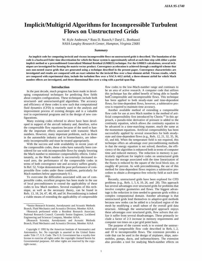
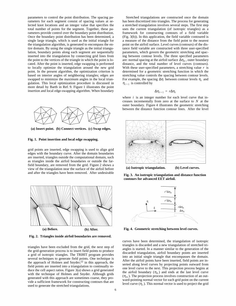
parameters to control the point distribution. The spacing pa-rameters for each segment consist of spacing values at se-lected knot locations and an integer value that specifies thetotal number of points for the segment. Together, these pa-rameters provide control over the boundary point distribution.Once the boundary point distribution has been determined, asingle large triangle, which is used as the initial triangle forthe triangulation algorithm, is generated to encompass the en-tire domain. By using the single triangle as the initial triangu-lation, boundary points along each segment are sequentiallyinserted into the triangulation by connecting grid lines fromthe point to the vertices of the triangle in which the point is lo-cated. After the point is inserted, edge swapping is performedto locally optimize the triangulation around the new gridpoint. In the present algorithm, the optimization criterion isbased on interior angles of neighboring triangles; edges areswapped to minimize the maximum angles in the local trian-gulation. This local optimization procedure is discussed inmore detail by Barth in Ref.9. Figure1 illustrates the pointinsertion and local edge-swapping algorithm. When boundary

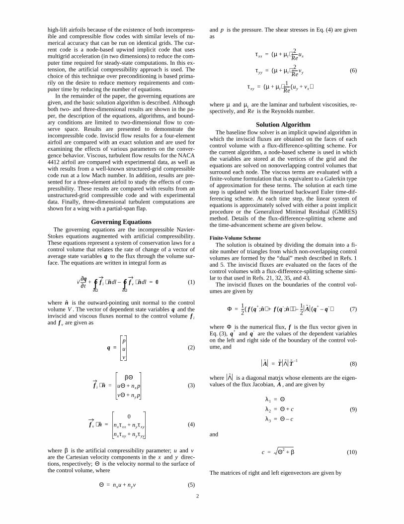
grid points are inserted, edge swapping is used to align gridedges with the boundary curve. After the domain boundariesare inserted, triangles outside the computational domain, suchas triangles inside the airfoil boundaries or outside the far-field boundary, are removed from the grid. Figure2 shows aview of the triangulation near the surface of the airfoil beforeand after the triangles have been removed. After undesirable

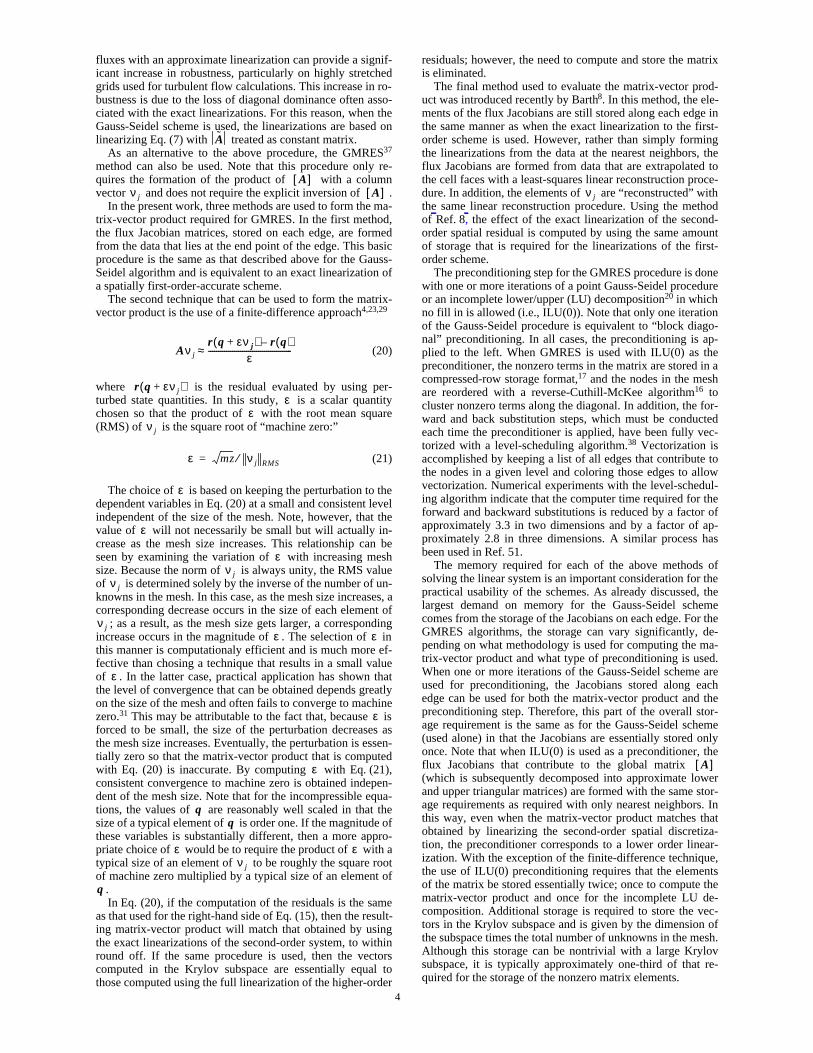
triangles have been excluded from the grid, the next step ofthe grid-generation process is to insert field points to producea grid of isotropic triangles. The TRI8IT program providesseveral techniques to generate field points. One technique isthe approach of Holmes and Snyder;22 in this approach, thefield points are inserted into a triangulation to continually re-duce the cell aspect ratios. Figure 3(a) shows a grid generatedwith the technique of Holmes and Snyder. Although gridsgenerated with this approach are sometimes coarse, they pro-vide a sufficient framework for constructing contours that areused to generate the stretched triangulations.

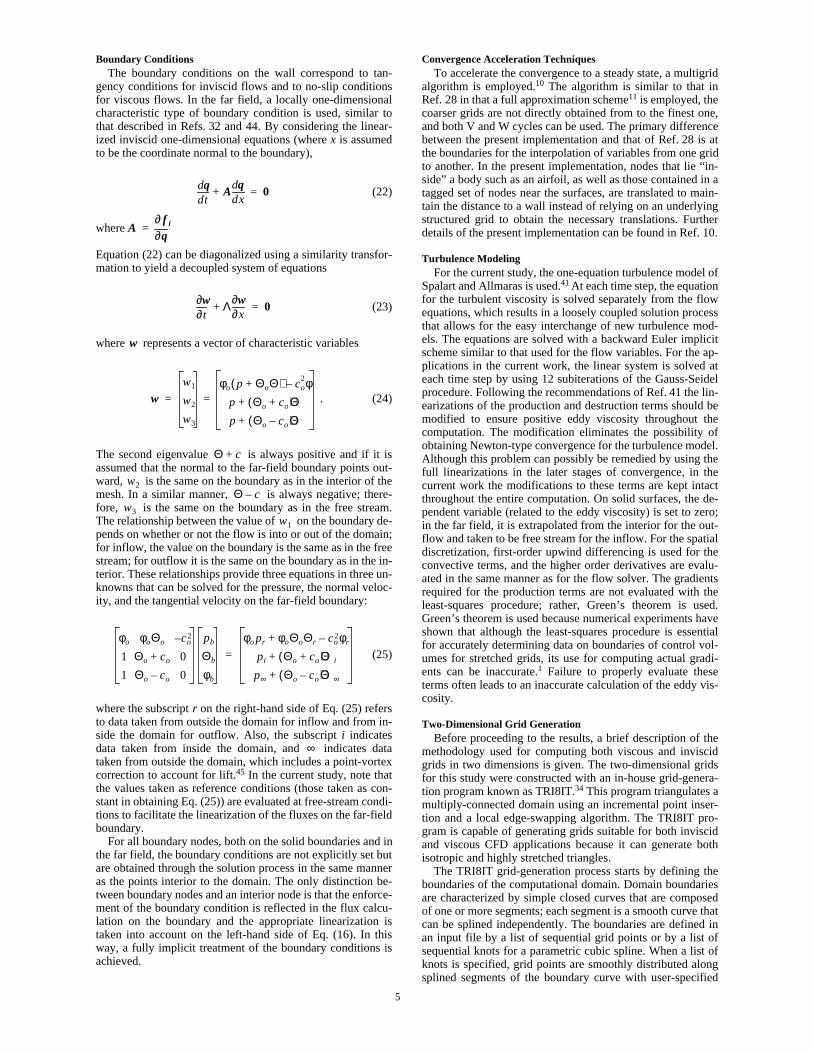
Stretched triangulations are constructed once the domainhas been discretized into triangles. The process for generatinga stretched triangulation involves several steps. The first stepuses the current triangulation (of isotropic triangles) as aframework for constructing contours of a field variable(Fig. 3(b)). In this application, the field variable contoured isa measure of the distance from the field point to the nearestpoint on the airfoil surface. Level curves (contours) of the dis-tance field variable are constructed with three user-specifiedparameters, which govern the geometric stretching and spac-ing between contour levels. The three specified parametersare: normal spacing at the airfoil surface , outer boundarydistance, and the total number of level curves (contours).With these user-specified parameters, a stretching value isdetermined for a geometric stretching function in which thestretching value controls the spacing between contour levels.For example, the spacing between contour levels and

is controlled by

where is an integer number for each level curve that in-creases incrementally from zero at the surface to at theouter boundary. Figure4 illustrates the geometric stretchingbetween the distance function contour lines. After the level

curves have been determined, the triangulation of isotropictriangles is discarded and a new triangulation of stretched tri-angles is started. In a manner similar to the generation of thediscarded triangulation, airfoil boundary points are insertedinto an initial single triangle that encompasses the domain.After the airfoil points have been inserted, field points are in-serted along level curves by projecting points outward fromone level curve to the next. This projection process begins atthe airfoil boundary ( ) and ends at the last level curve( ). The projection process involves construction of an out-ward-pointing normal vector for each grid point on the currentlevel curve ( ). This normal vector is used to project the grid

Fig. 1. Point insertion and local edge swapping.

Fig. 2. Triangles inside airfoil boundaries are removed.

(a) Insert point. (b) Connect vertices. (c) Swap edges.

(a) Before. (b) After.

Fig. 3. An isotropic triangulation and distance functioncontours for advanced EET airfoil.

Fig. 4. Geometric stretching between level curves.

∆η0

r

∆η ηiηi 1+

∆ηi 1+ r∆ηi=

iN

(a) Isotropic triangulation. (b) Level curves.

η

ξ∆η0

r ∆η0

r 2∆η0

r 3∆η0

η0ηN

ηi

7

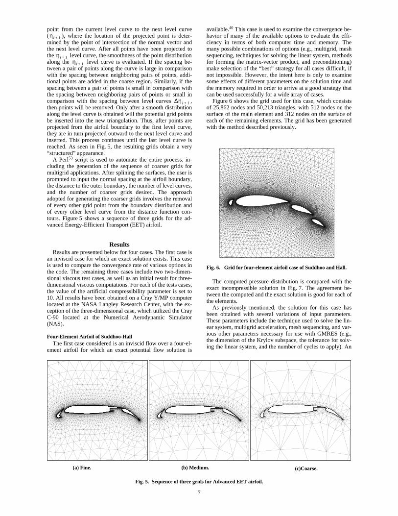
Fig. 5. Sequence of three grids for Advanced EET airfoil.

(a) Fine. (b) Medium. (c)Coarse.

point from the current level curve to the next level curve( ), where the location of the projected point is deter-mined by the point of intersection of the normal vector andthe next level curve. After all points have been projected tothe level curve, the smoothness of the point distributionalong the level curve is evaluated. If the spacing be-tween a pair of points along the curve is large in comparisonwith the spacing between neighboring pairs of points, addi-tional points are added in the coarse region. Similarly, if thespacing between a pair of points is small in comparison withthe spacing between neighboring pairs of points or small incomparison with the spacing between level curves ,then points will be removed. Only after a smooth distributionalong the level curve is obtained will the potential grid pointsbe inserted into the new triangulation. Thus, after points areprojected from the airfoil boundary to the first level curve,they are in turn projected outward to the next level curve andinserted. This process continues until the last level curve isreached. As seen in Fig.5, the resulting grids obtain a very“structured” appearance.

A Perl53 script is used to automate the entire process, in-cluding the generation of the sequence of coarser grids formultigrid applications. After splining the surfaces, the user isprompted to input the normal spacing at the airfoil boundary,the distance to the outer boundary, the number of level curves,and the number of coarser grids desired. The approachadopted for generating the coarser grids involves the removalof every other grid point from the boundary distribution andof every other level curve from the distance function con-tours. Figure5 shows a sequence of three grids for the ad-vanced Energy-Efficient Transport (EET) airfoil.

ResultsResults are presented below for four cases. The first case is

an inviscid case for which an exact solution exists. This caseis used to compare the convergence rate of various options inthe code. The remaining three cases include two two-dimen-sional viscous test cases, as well as an initial result for three-dimensional viscous computations. For each of the tests cases,the value of the artificial compressibility parameter is set to10. All results have been obtained on a Cray Y/MP computerlocated at the NASA Langley Research Center, with the ex-ception of the three-dimensional case, which utilized the CrayC-90 located at the Numerical Aerodynamic Simulator(NAS).

Four-Element Airfoil of Suddhoo-HallThe first case considered is an inviscid flow over a four-el-

ement airfoil for which an exact potential flow solution is

available.40 This case is used to examine the convergence be-havior of many of the available options to evaluate the effi-ciency in terms of both computer time and memory. Themany possible combinations of options (e.g., multigrid, meshsequencing, techniques for solving the linear system, methodsfor forming the matrix-vector product, and preconditioning)make selection of the “best” strategy for all cases difficult, ifnot impossible. However, the intent here is only to examinesome effects of different parameters on the solution time andthe memory required in order to arrive at a good strategy thatcan be used successfully for a wide array of cases.

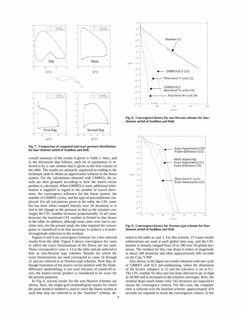
Figure6 shows the grid used for this case, which consistsof 25,862 nodes and 50,213 triangles, with 512 nodes on thesurface of the main element and 312 nodes on the surface ofeach of the remaining elements. The grid has been generatedwith the method described previously.

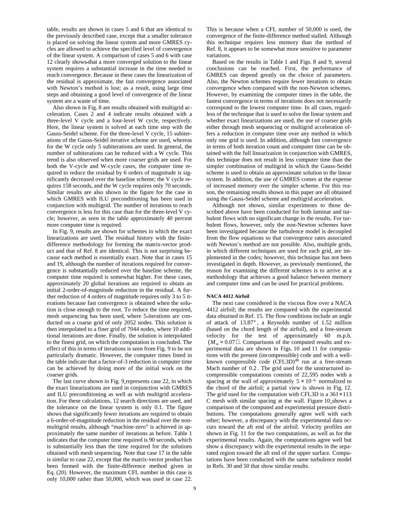
The computed pressure distribution is compared with theexact incompressible solution in Fig.7. The agreement be-tween the computed and the exact solution is good for each ofthe elements.

As previously mentioned, the solution for this case hasbeen obtained with several variations of input parameters.These parameters include the technique used to solve the lin-ear system, multigrid acceleration, mesh sequencing, and var-ious other parameters necessary for use with GMRES (e.g.,the dimension of the Krylov subspace, the tolerance for solv-ing the linear system, and the number of cycles to apply). An

ηi 1+

ηi 1+ηi 1+

∆ηi 1+

Fig. 6. Grid for four-element airfoil case of Suddhoo and Hall.

8

overall summary of the results is given in Table1. Here, andin the discussion that follows, each set of parameters is re-ferred to by a case number that is given in the first column ofthe table. The results are primarily organized according to thetechnique used to obtain an approximate solution to the linearsystem. For the calculations obtained with GMRES, the re-sults are then grouped according to how the matrix-vectorproduct is calculated. When GMRES is used, additional infor-mation is supplied in regard to the number of search direc-tions, the convergence tolerance for the linear system, thenumber of GMRES cycles, and the type of preconditioner em-ployed. For all calculations given in the table, the CFL num-ber has been either ramped linearly over 50 iterations or istied to the change in the pressure so that as the solution con-verges the CFL number increases proportionally. In all cases,however, the maximum CFL number is limited to that shownin the table. In addition, although most cases were run to ma-chine zero, for the present study the time required for conver-gence is considered to be that necessary to achieve a 6-order-of-magnitude reduction in the residual.

Figures8 and 9 are convergence histories for a few selectedresults from the table. Figure 8 shows convergence for casesin which the exact linearizations of the fluxes are not used.These correspond to cases 1-13 in the table and are referred tohere as non-Newton type schemes. Results for which theexact linearizations are used correspond to cases 14 through22 and are referred to as Newton-type schemes. Note that, al-though formation of the matrix-vector product with the finite-difference methodology is not exact because of round-off er-rors, the matrix-vector product is considered to be exact forthe present purposes.

In Fig.8, several results for the non-Newton schemes areshown. Here, the single-grid (nonmultigrid) results for whichthe point iterative method is used to solve the linear system ateach time step are referred to as the “baseline” scheme, de-

noted in the table as case 1. For this scheme, 15 Gauss-Seidelsubiterations are used at each global time step, and the CFLnumber is linearly ramped from 10 to 200 over 50 global iter-ations. The residual for this case drops 6 orders of magnitudein about 540 iterations and takes approximately 600 secondson the Cray Y/MP

Also shown in the figure are results obtained with one cycleof GMRES with ILU preconditioning, where the dimensionof the Krylov subspace is 12 and the tolerance is set to 0.1.The CFL number for this case has been allowed to go as highas 50,000 and is increased as the solution converges. Here, theresidual drops much faster; only 142 iterations are required toobtain the convergence criteria. For this case, the computertime is reduced over the baseline scheme; approximately 419seconds are required to reach the convergence criteria. In the

Fig. 7. Comparison of computed and exact pressure distributionfor four-element airfoil of Suddhoo and Hall.

p

Cp

x c⁄

x c⁄

x c⁄

x c⁄

Slat Main

First flap Second flap

Fig. 8. Convergence history for non-Newton schemes for four-element airfoil of Suddhoo and Hall.

Fig. 9. Convergence history for Newton-type schemes for four-element airfoil of Suddhoo and Hall.

Baseline (1)

GMRES/ILU (12)

Three-level V-cycle (2)

GMRES/ILU

Four-level W-cycle (4)

three-level V-cycle (13)

Exact linearization (19)

Mesh sequencing:Exact linearization (21)Finite-difference (16)

Three-level V-cycle:Exact linearization (22)

Finite-difference (15)

9

table, results are shown in cases 5 and 6 that are identical tothe previously described case, except that a smaller toleranceis placed on solving the linear system and more GMRES cy-cles are allowed to achieve the specified level of convergenceof the linear system. A comparison of cases 5 and 6 with case12 clearly showsthat a more converged solution to the linearsystem requires a substantial increase in the time needed toreach convergence. Because in these cases the linearization ofthe residual is approximate, the fast convergence associatedwith Newton’s method is lost; as a result, using large timesteps and obtaining a good level of convergence of the linearsystem are a waste of time.

Also shown in Fig.8 are results obtained with multigrid ac-celeration. Cases 2 and 4 indicate results obtained with athree-level V cycle and a four-level W cycle, respectively.Here, the linear system is solved at each time step with theGauss-Seidel scheme. For the three-level V cycle, 15 subiter-ations of the Gauss-Seidel iterative scheme are used, whereasfor the W cycle only 5 subiterations are used. In general, thenumber of subiterations can be reduced with a W cycle. Thistrend is also observed when more coarser grids are used. Forboth the V-cycle and W-cycle cases, the computer time re-quired to reduce the residual by 6 orders of magnitude is sig-nificantly decreased over the baseline scheme; the V cycle re-quires 158 seconds, and the W cycle requires only 70 seconds.Similar results are also shown in the figure for the case inwhich GMRES with ILU preconditioning has been used inconjunction with multigrid. The number of iterations to reachconvergence is less for this case than for the three-level V cy-cle; however, as seen in the table approximately 40 percentmore computer time is required.

In Fig. 9, results are shown for schemes in which the exactlinearizations are used. The residual history with the finite-difference methodology for forming the matrix-vector prod-uct and that of Ref.8 are identical. This is not surprising be-cause each method is essentially exact. Note that in cases 15and 19, although the number of iterations required for conver-gence is substantially reduced over the baseline scheme, thecomputer time required is somewhat higher. For these cases,approximately 20 global iterations are required to obtain aninitial 2-order-of-magnitude reduction in the residual. A fur-ther reduction of 4 orders of magnitude requires only 3 to 5 it-erations because fast convergence is obtained when the solu-tion is close enough to the root. To reduce the time required,mesh sequencing has been used, where 5iterations are con-ducted on a coarse grid of only 2052 nodes. This solution isthen interpolated to a finer grid of 7044 nodes, where 10 addi-tional iterations are done. Finally, the solution is interpolatedto the finest grid, on which the computation is concluded. Theeffect of this in terms of iterations is seen from Fig.9 to be notparticularly dramatic. However, the computer times listed inthe table indicate that a factor-of-3 reduction in computer timecan be achieved by doing more of the initial work on thecoarser grids.

The last curve shown in Fig.9 represents case 22, in whichthe exact linearizations are used in conjunction with GMRESand ILU preconditioning as well as with multigrid accelera-tion. For these calculations, 12 search directions are used, andthe tolerance on the linear system is only 0.1. The figureshows that significantly fewer iterations are required to obtaina 6-order-of-magnitude reduction in the residual over the non-multigrid results, although “machine-zero” is achieved in ap-proximately the same number of iterations as before. Table 1indicates that the computer time required is 90 seconds, whichis substantially less than the time required for the solutionsobtained with mesh sequencing. Note that case 17 in the tableis similar to case 22, except that the matrix-vector product hasbeen formed with the finite-difference method given inEq.(20). However, the maximum CFL number in this case isonly 10,000 rather than 50,000, which was used in case 22.

This is because when a CFL number of 50,000 is used, theconvergence of the finite-difference method stalled. Althoughthis technique requires less memory than the method ofRef.8, it appears to be somewhat more sensitive to parametervariations.

Based on the results in Table1 and Figs.8 and 9, severalconclusions can be reached. First, the performance ofGMRES can depend greatly on the choice of parameters.Also, the Newton schemes require fewer iterations to obtainconvergence when compared with the non-Newton schemes.However, by examining the computer times in the table, thefastest convergence in terms of iterations does not necessarilycorrespond to the lowest computer time. In all cases, regard-less of the technique that is used to solve the linear system andwhether exact linearizations are used, the use of coarser gridseither through mesh sequencing or multigrid acceleration of-fers a reduction in computer time over any method in whichonly one grid is used. In addition, although fast convergencein terms of both iteration count and computer time can be ob-tained with the full linearization in conjunction with GMRES,this technique does not result in less computer time than thesimpler combination of multigrid in which the Gauss-Seidelscheme is used to obtain an approximate solution to the linearsystem. In addition, the use of GMRES comes at the expenseof increased memory over the simpler scheme. For this rea-son, the remaining results shown in this paper are all obtainedusing the Gauss-Seidel scheme and multigrid acceleration.

Although not shown, similar experiments to those de-scribed above have been conducted for both laminar and tur-bulent flows with no significant change in the results. For tur-bulent flows, however, only the non-Newton schemes havebeen investigated because the turbulence model is decoupledfrom the flow equations so that convergence rates associatedwith Newton’s method are not possible. Also, multiple grids,in which different techniques are used for each grid, are im-plemented in the codes; however, this technique has not beeninvestigated in depth. However, as previously mentioned, thereason for examining the different schemes is to arrive at amethodology that achieves a good balance between memoryand computer time and can be used for practical problems.

NACA 4412 AirfoilThe next case considered is the viscous flow over a NACA

4412 airfoil; the results are compared with the experimentaldata obtained in Ref.15. The flow conditions include an angleof attack of , a Reynolds number of 1.52 million(based on the chord length of the airfoil), and a free-streamvelocity for the test of approximately 60 m.p.h.

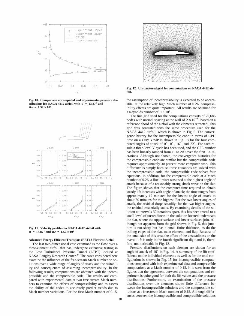
. Comparisons of the computed results and ex-perimental data are shown in Figs.10 and11 for computa-tions with the present (incompressible) code and with a well-known compressible code (CFL3D)46 run at a free-streamMach number of . The grid used for the unstructured in-compressible computations consists of 22,595 nodes with aspacing at the wall of approximately normalized tothe chord of the airfoil; a partial view is shown in Fig.12.The grid used for the computation with CFL3D is a 361×113C mesh with similar spacing at the wall. Figure10 shows acomparison of the computed and experimental pressure distri-butions. The computations generally agree well with eachother; however, a discrepancy with the experimental data oc-curs toward the aft end of the airfoil. Velocity profiles areshown in Fig.11 for the two computations, as well as for theexperimental results. Again, the computations agree well butshow a discrepancy with the experimental results in the sepa-rated region toward the aft end of the upper surface. Compu-tations have been conducted with the same turbulence modelin Refs. 30 and 50 that show similar results.

13.87°

M∞ 0.07≈( )

0.2

5 10 6–×

10

Advanced Energy Efficient Transport (EET) 3-Element AirfoilThe last two-dimensional case examined is the flow over a

three-element airfoil that has undergone extensive testing inthe Low Turbulence Pressure Tunnel (LTPT) located atNASA Langley Research Center.25 The cases considered hereexamine the influence of the free-stream Mach number on so-lutions over a wide range of angles of attack and the suitabil-ity and consequences of assuming incompressibility. In thefollowing results, computations are obtained with the incom-pressible and the compressible code. The results are com-pared with experimental data at two free-stream Mach num-bers to examine the effects of compressibility and to assessthe ability of the codes to accurately predict trends due toMach-number variations. For the first Mach number of 0.15,

the assumption of incompressibility is expected to be accept-able; at the relatively high Mach number of 0.26, compress-ibility effects are quite important. All results are obtained fora Reynolds number of .

The fine grid used for the computations consists of 70,686nodes with normal spacing at the wall of , based on areference chord of the airfoil with the elements retracted. Thisgrid was generated with the same procedure used for theNACA 4412 airfoil, which is shown in Fig.5. The conver-gence history for the incompressible code in terms of CPUtime on a Cray Y/MP is shown in Fig.13 for the four com-puted angles of attack of , , , and . For each re-sult, a three-level V cycle has been used, and the CFL numberhas been linearly ramped from 10 to 200 over the first 100 it-erations. Although not shown, the convergence histories forthe compressible code are similar but the compressible coderequires approximately 30 percent more computer time. Thisdifference is simply because three equations are solved withthe incompressible code; the compressible code solves fourequations. In addition, for the compressible code at a Machnumber of 0.26, a flux limiter was used at the highest angle ofattack because of a reasonably strong shock wave on the slat.The figure shows that the computer time required to obtainsteady lift increases with angle of attack; the time ranges fromapproximately 12 minutes for the lowest angle of attack toabout 30 minutes for the highest. For the two lower angles ofattack, the residual drops steadily; for the two higher angles,the residual essentially stalls. By examining details of the so-lution at intervals 50 iterations apart, this has been traced to asmall level of unsteadiness in the solution located underneaththe slat, where the upper surface and lower surfaces join. Al-though not apparent from the grid shown in Fig.5, this junc-ture is not sharp but has a small finite thickness, as do thetrailing edges of the slat, main element, and flap. Because ofthe small size of this area, the effect of the unsteadiness on theoverall lift is only in the fourth significant digit and is, there-fore, not noticeable in Fig. 13.

Pressure distributions on each element are shown for anangle of attack of in Fig. 14. A summary of the lift coef-ficients on the individual elements as well as for the total con-figuration is shown in Fig.15 for incompressible computa-tions compared with both experimental data and compressiblecomputations at a Mach number of 0.15. It is seen from thefigures that the agreement between the computations and ex-periment is quite good for both the lift values and the pressuredistributions. Furthermore, an examination of the pressuredistributions over the elements shows little difference be-tween the incompressible solutions and the compressible so-lutions at a freestream Mach number of 0.15. Although differ-ences between the incompressible and compressible solutions

Fig. 10. Comparison of computed and experimental pressure dis-tributions for NACA 4412 airfoil with and

.

Fig. 11. Velocity profiles for NACA 4412 airfoil withand .

α 13.87°=Re 1.52 106×=

α 13.87°= Re 1.52 106×=

Fig. 12. Unstructured grid for computations on NACA 4412 air-foil.

9 106×

2 10 6–×

0° 8° 16° 22°

16°

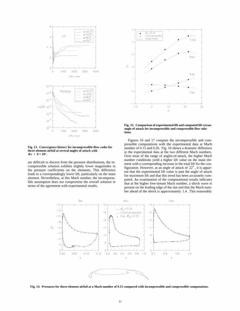
Fig. 14. Pressures for three-element airfoil at a Mach number of 0.15 compared with incompressible and compressible computations.

11

are difficult to discern from the pressure distributions, the in-compressible solution exhibits slightly lower magnitudes inthe pressure coefficients on the elements. This differenceleads to a correspondingly lower lift, particularly on the mainelement. Nevertheless, at this Mach number, the incompress-ible assumption does not compromise the overall solution interms of the agreement with experimental results.

Figures 16 and 17 compare the incompressible and com-pressible computations with the experimental data at Machnumber of 0.15 and 0.26. Fig. 16 shows a dramatic differencein the experimental data at the two different Mach numbers.Over most of the range of angles-of-attack, the higher Machnumber conditions yield a higher lift value on the main ele-ment with a corresponding increase in the total lift for the con-figuration. However, at an angle of attack of , it is appar-ent that the experimental lift value is past the angle of attackfor maximum lift and that this trend has been accurately com-puted. An examination of the computational results indicatesthat at the higher free-stream Mach number, a shock wave ispresent on the leading edge of the slat and that the Mach num-ber ahead of the shock is approximately . This reasonably

Fig. 13. Convergence history for incompressible-flow codes forthree-element airfoil at several angles of attack with

.Re 9 106×=

Fig. 15. Comparison of experimental lift and computed lift versusangle of attack for incompressible and compressible flow solu-tions.

22o

1.4

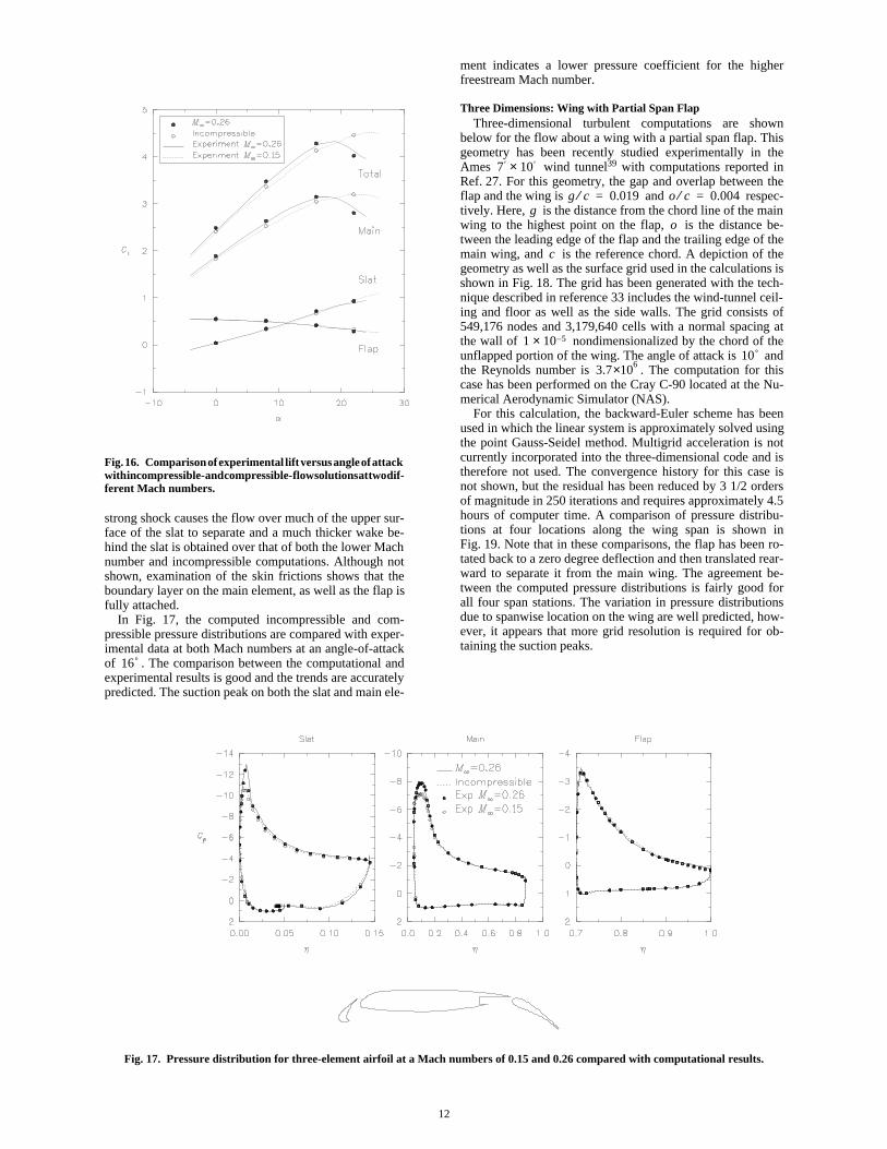
Fig. 17. Pressure distribution for three-element airfoil at a Mach numbers of 0.15 and 0.26 compared with computational results.

12

strong shock causes the flow over much of the upper sur-face of the slat to separate and a much thicker wake be-hind the slat is obtained over that of both the lower Machnumber and incompressible computations. Although notshown, examination of the skin frictions shows that theboundary layer on the main element, as well as the flap isfully attached.

In Fig. 17, the computed incompressible and com-pressible pressure distributions are compared with exper-imental data at both Mach numbers at an angle-of-attackof . The comparison between the computational andexperimental results is good and the trends are accuratelypredicted. The suction peak on both the slat and main ele-

Fig. 16. Comparison of experimental lift versus angle of attackwith incompressible- and compressible- flow solutions at two dif-ferent Mach numbers.

16°

ment indicates a lower pressure coefficient for the higherfreestream Mach number.

Three Dimensions: Wing with Partial Span FlapThree-dimensional turbulent computations are shown

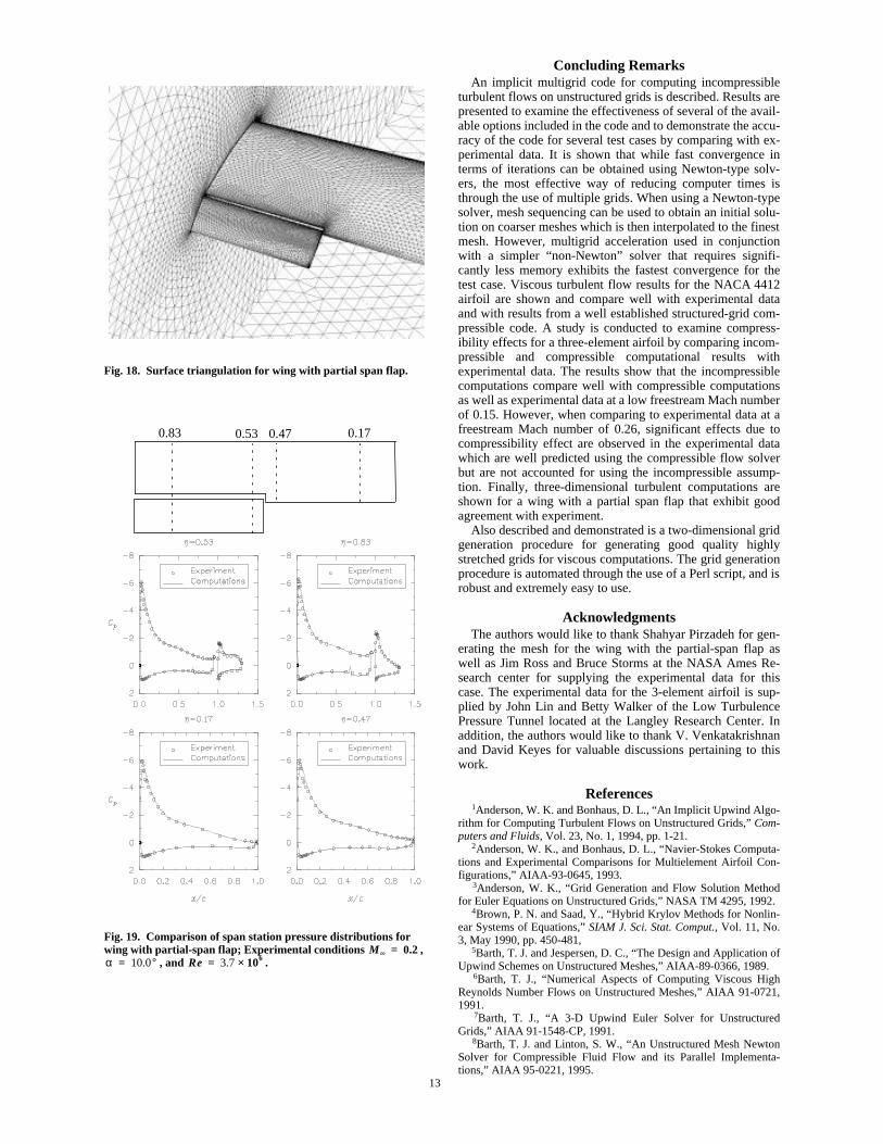
below for the flow about a wing with a partial span flap. Thisgeometry has been recently studied experimentally in theAmes wind tunnel39 with computations reported inRef.27. For this geometry, the gap and overlap between theflap and the wing is and respec-tively. Here, is the distance from the chord line of the mainwing to the highest point on the flap, is the distance be-tween the leading edge of the flap and the trailing edge of themain wing, and is the reference chord. A depiction of thegeometry as well as the surface grid used in the calculations isshown in Fig.18. The grid has been generated with the tech-nique described in reference 33 includes the wind-tunnel ceil-ing and floor as well as the side walls. The grid consists of549,176 nodes and 3,179,640 cells with a normal spacing atthe wall of nondimensionalized by the chord of theunflapped portion of the wing. The angle of attack is andthe Reynolds number is . The computation for thiscase has been performed on the Cray C-90 located at the Nu-merical Aerodynamic Simulator (NAS).

For this calculation, the backward-Euler scheme has beenused in which the linear system is approximately solved usingthe point Gauss-Seidel method. Multigrid acceleration is notcurrently incorporated into the three-dimensional code and istherefore not used. The convergence history for this case isnot shown, but the residual has been reduced by 3 1/2 ordersof magnitude in 250 iterations and requires approximately 4.5hours of computer time. A comparison of pressure distribu-tions at four locations along the wing span is shown inFig. 19. Note that in these comparisons, the flap has been ro-tated back to a zero degree deflection and then translated rear-ward to separate it from the main wing. The agreement be-tween the computed pressure distributions is fairly good forall four span stations. The variation in pressure distributionsdue to spanwise location on the wing are well predicted, how-ever, it appears that more grid resolution is required for ob-taining the suction peaks.

7′ 10× ′

g c⁄ 0.019= o c⁄ 0.004=g

o

c

1 10 5–×10°

3.7 6×10

13

Concluding RemarksAn implicit multigrid code for computing incompressible

turbulent flows on unstructured grids is described. Results arepresented to examine the effectiveness of several of the avail-able options included in the code and to demonstrate the accu-racy of the code for several test cases by comparing with ex-perimental data. It is shown that while fast convergence interms of iterations can be obtained using Newton-type solv-ers, the most effective way of reducing computer times isthrough the use of multiple grids. When using a Newton-typesolver, mesh sequencing can be used to obtain an initial solu-tion on coarser meshes which is then interpolated to the finestmesh. However, multigrid acceleration used in conjunctionwith a simpler “non-Newton” solver that requires signifi-cantly less memory exhibits the fastest convergence for thetest case. Viscous turbulent flow results for the NACA4412airfoil are shown and compare well with experimental dataand with results from a well established structured-grid com-pressible code. A study is conducted to examine compress-ibility effects for a three-element airfoil by comparing incom-pressible and compressible computational results withexperimental data. The results show that the incompressiblecomputations compare well with compressible computationsas well as experimental data at a low freestream Mach numberof 0.15. However, when comparing to experimental data at afreestream Mach number of 0.26, significant effects due tocompressibility effect are observed in the experimental datawhich are well predicted using the compressible flow solverbut are not accounted for using the incompressible assump-tion. Finally, three-dimensional turbulent computations areshown for a wing with a partial span flap that exhibit goodagreement with experiment.

Also described and demonstrated is a two-dimensional gridgeneration procedure for generating good quality highlystretched grids for viscous computations. The grid generationprocedure is automated through the use of a Perl script, and isrobust and extremely easy to use.

AcknowledgmentsThe authors would like to thank Shahyar Pirzadeh for gen-

erating the mesh for the wing with the partial-span flap aswell as Jim Ross and Bruce Storms at the NASA Ames Re-search center for supplying the experimental data for thiscase. The experimental data for the 3-element airfoil is sup-plied by John Lin and Betty Walker of the Low TurbulencePressure Tunnel located at the Langley Research Center. Inaddition, the authors would like to thank V. Venkatakrishnanand David Keyes for valuable discussions pertaining to thiswork.

References 1Anderson, W. K. and Bonhaus, D. L., “An Implicit Upwind Algo-

rithm for Computing Turbulent Flows on Unstructured Grids,”Com-puters and Fluids, Vol. 23, No. 1, 1994, pp. 1-21.

2Anderson, W. K., and Bonhaus, D. L., “Navier-Stokes Computa-tions and Experimental Comparisons for Multielement Airfoil Con-figurations,” AIAA-93-0645, 1993.

3Anderson, W. K., “Grid Generation and Flow Solution Methodfor Euler Equations on Unstructured Grids,” NASA TM 4295, 1992.

4Brown, P. N. and Saad, Y., “Hybrid Krylov Methods for Nonlin-ear Systems of Equations,”SIAM J. Sci. Stat. Comput., Vol. 11, No.3, May 1990, pp. 450-481,

5Barth, T. J. and Jespersen, D. C., “The Design and Application ofUpwind Schemes on Unstructured Meshes,” AIAA-89-0366, 1989.

6Barth, T. J., “Numerical Aspects of Computing Viscous HighReynolds Number Flows on Unstructured Meshes,” AIAA 91-0721,1991.

7Barth, T. J., “A 3-D Upwind Euler Solver for UnstructuredGrids,” AIAA 91-1548-CP, 1991.

8Barth, T. J. and Linton, S. W., “An Unstructured Mesh NewtonSolver for Compressible Fluid Flow and its Parallel Implementa-tions,” AIAA 95-0221, 1995.

Fig. 18. Surface triangulation for wing with partial span flap.

Fig. 19. Comparison of span station pressure distributions forwing with partial-span flap; Experimental conditions ,

, and .

0.170.470.530.83

M ∞ 0.2=α 10.0°= Re 3.7 106×=

14

9Barth, T. J., “Steiner Triangulation for Isotropic and Stretched El-ements,” AIAA 95-0213, 1995.

10Bonhaus, D. L., “An Upwind Multigrid Method for Solving Vis-cous Flows on Unstructured Triangular Meshes,” M.S. Thesis,George Washington University, 1993.

11Brandt, A., “Multilevel Adaptive Computations in Fluid Dynam-ics,” AIAA J., Vol. 18, No. 10, Oct. 1980, pp. 1165-1172.

12Cao, H. V. and Kusunose, K., “Grid Generation and Navier-Stokes Analysis for Multi-Element Airfoils,” AIAA 94-0748, 1994.

13Choi, Y. H. and Merkle, C. L., “The Application of Precondition-ing in Viscous Flows,”J. Comp. Phys., Vol. 105, 1993, pp. 207-233.

14Chorin, A. J., “A Numerical Method for Solving IncompressibleViscous Flow Problems,”J. Comp. Phys., Vol. 2, Aug. 1967, pp. 12-26.

15Coles, D. and Wadcock, A. J., “Flying-Hot-Wire Study of FlowPast an NACA 4412 Airfoil at Maximum Lift,” AIAA Journal, Vol.17, No. 4, April 1979.

16Cuthill, E. and McKee, J., “Reducing the Band Width of SparseSymmetric Matrices.” Proc. ACM National Conference, 157 (1969).

17George, A. and Liu, J. W.,Computer Solution of Large SparsePositive Definite Systems, Prentice Hall Series in ComputationalMathematics, Englewood Cliffs, N. J., 1981.

18Godfrey, A. G., “Topics on Spatially High-Order AccurateMethods and Preconditioning of the Navier-Stokes Equations with Fi-nite-Rate Chemistry,” Ph.D. Thesis, Virginia Polytechnic Instituteand State University, 1992.

19Golub, G. H. and Van Loan, C. F. “Matrix Computations,” JohnHopkins University Press, 1991.

20Hackbusch, W.,Iterative Solution of Large Sparse Systems ofEquations, Springer-Verlag, New York, 1994.

21Hartwich, P. M. and Hsu, C., “An Implicit Flux-Difference Split-ting Scheme for Three-Dimensional, Incompressible Navier-StokesSolutions to Leading Edge Vortex Flows,” AIAA 86-1839-CP, 1986.

22Holmes, D. G. and Snyder, D. D. “The Generation of Unstruc-tured Triangular Meshes Using Delaunay Triangulation,” NumericalGrid Generation in Computational Fluid Mechanics ‘88, (S. Sen-gupta, J. Hauser, P. R. Eiseman, and J. F. Thompson, eds.), PineridgePress, 1988, pp. 643-652.

23Johan, Z. and Hughes, J. R., “A Globally Convergent Matrix-Free Algorithm for Implicit Time-Marching Schemes Arising in Fi-nite Element Analysis in Fluids,” Computer Methods in Applied Me-chanics and Engineering, Vol. 87, 1991, pp. 281-304.

24Jorgenson, P. C. E., and Pletcher, R. H., “An Implicit NumericalScheme for the Simulation of Internal Viscous Flows on UnstructuredGrids,” AIAA 94-0306, 1994.

25Lin, J. C. and Dominick, C. J., “Optimization of an AdvancedDesign Three-Element Airfoil at High Reynolds Numbers,” AIAA95-1858, 1995.

26Marcum, D. L. and Agarwal, R., “A Three-Dimensional FiniteElement Navier-Stokes Solver with Turbulence Model for Un-structured Grids,” AIAA 90-1652, 1990.

27Mathias, D. L., Roth, K. R., Ross, J. C., Rogers, S. E., and Cum-mings, R. M., “Navier-Stokes Analysis of the Flow About a FlapEdge,” AIAA 95-0185, 1995.

28Mavriplis, D., “Turbulent Flow Calculation using Unstructuredand Adaptive Meshes,”Int. J. Numer. Meth. Fluids, Vol.13, 1991.

29McHugh, P. R. and Knoll, D. A., “Comparison of Standard andMatrix-free Implementations of Several Newton-Krylov Solvers,”AIAA Journal, Vol. 32, No. 12, 1994, pp. 2394-2400.

30Mentor, F. R., “Zonal Two-Equation Turbulence Modelsfor Aerodynamic Flows,” AIAA 93-2906, 1993.

31Nielsen, E. Anderson, W. K., Walters, R., and Keyes, D., “Appli-cation of Newton-Krylov Methodology to a Three-Dimensional Un-structured Euler Code,” AIAA 95-1733.

32Pan, D. and Chakravarty, S., “Unified Formulation for Incom-pressible Flows,” AIAA 89-0122, 1989.

33Pirzadeh, S., “Viscous Unstructured Three-Dimensional Gridsby the Advancing-Layers Method,” AIAA 94-0417, 1994

34Rausch, R. D., “TRI8IT: An Unstructured-Grid Generation Pro-gram for Two-Dimensional Domains,” Report in preparation.

35Rogers, S. E. and Kwak, D., “An Upwind Differencing Schemefor the Time-Accurate Incompressible Navier-Stokes Equations,”AIAA 85-2583-CP, 1985.

36Rogers, S. E., “Progress in High-Lift Aerodynamic Calcula-tions,” AIAA 93-0194, 1993.

37Saad, Y., and Schultz, M. H., “GMRES: A Generalized MinimalResidual Algorithm for Solving Nonsymmetric Linear Systems,”SIAM J. Sci. Stat. Comput., Vol. 7, 1986.

38Saad, Y., “Krylov Subspace Methods on Supercomputers,”SIAM J. Sci. Stat. Comput., Vol. 10, No. 6, 1989, pp. 1200-1232.

39Storms, Bruce, L. and Ross, James C., “An Experimental Studyof a Simple Wing with a Part-Span Flap,” NASA TM in preparation.

40Suddhoo, A., and Hall, I. M., “Test Cases for the Plane PotentialFlow Past Multi-Element Airfoils,”Aeronautical Journal, Dec. 1985.

41Spalart, P. R., and Allmaras, S. R., “A One-Equation TurbulenceModel for Aerodynamic Flows,” AIAA 92-0439, 1992.

42Taylor, L. K., “Unsteady Three-Dimensional Incompressible Al-gorithm Based on Artificial Compressibility,” Ph.D. Thesis, Missis-sippi State University, 1991.

43Taylor, L. K. and Whitfield, David L., “Unsteady Three-Dimen-sional Incompressible Euler and Navier-Stokes Solver for Stationaryand Dynamic Grids,” AIAA-91-1650, 1991.

44Taylor, L. K., Busby, J. A., Jiang, M. Y., Arabshahi, A., Sreeni-vas, K., and Whitfield, D. L., “Time Accurate Incompressible Navier-Stokes Simulation of the Flapping Foil Experiment,” Presented at theSixth International Conference on Numerical Ship Hydrodynamics,Aug. 2-5, 1993.

45Thomas, J. L. and Salas, M. D., “Far-Field Boundary Conditionsfor Transonic Lifting Solutions to the Euler Equations,”AIAA Jour-nal, Vol. 24, No. 7, July 1986.

46Thomas, J., Krist, S., and Anderson, W. K., “Navier-StokesComputations of Vortical Flows Over Low-Aspect-Ratio Wings,”AIAA Journal, vol. 28, no. 2,1990, pp. 205-212.

47Turkel, E., “Preconditioned Methods for Solving the Incom-pressible and Low Speed Compressible Equations,”J. Comp. Phys.,Vol. 72, 1987, pp. 277-298.

48Turkel, E., “Review of Preconditioning Methods for Fluid Dy-namics,” ICASE Report No. 86-14, 1986.

49Van Leer, B., Lee, W., and Roe, P., “Characteristic Time-Step-ping or Local Preconditioning of the Euler Equations,” AIAA 91-1552-CP, 1991.

50Vatsa, V. N., Sanetrik, M. D., Parlette, E. B., Eiseman, P., andCheng, Z., “Multi-block Structured Grid Approach for Solving Flowsover Complex Aerodynamic Configurations,” AIAA-94-0655, 1994.

51Venkatakrishnan, V. and Mavriplis, D. J., “Implicit Solvers forUnstructured Meshes,” J. of Comp. Phys., Vol. 105, No. 1, June,1993, pp. 83-91.

52Volpe, G., “On the Use and Accuracy of Compressible FlowCodes at Low Mach Numbers,” AIAA-91-1662, 1991.

53Wall, Larry,Programming Perl, O’Reilly & Associates, 1990. 54Weiss, J. M. and Smith, W.A., “Preconditioning Applied to Vari-

able and Constant Density Time-Accurate Flows on UnstructuredMeshes,” AIAA 94-2209, 1994.

k ε–

k ω–

aNumbers in this column indicate the following0 indicates exact linearization of first-order system (nearest neighbors).1 indicates Newton-Krylov method (finite difference of residual).2 indicates exact linearizations for higher order system with method of reference 8.

Casenumber

LinearSolver

Matrix-Vectorproduct

aCFL1/CFL2

Ramp ofCFL

SearchDirections

GMRESCycles Tolerance ILU

Gauss-Seidel

iterations CPU Comment

1 GS NA 10/200 linear/50 NA NA NA NA 15 598 Baseline

2 GS NA 10/200 linear/50 NA NA NA NA 15 158 3-level V-cycle

3 GS NA 10/200 linear/50 NA NA NA NA 10 114 3-level W-cycle

4 GS NA 10/500 linear/50 NA NA NA NA 5 70 4-level W-cycle

5 GMRES 0 100/50K 12 10 0.001 1 NA 1469

6 GMRES 0 100/50K 12 3 0.001 1 NA 761

7 GMRES 0 10/200 linear/50 10 3 0.1 0 1 660 Diagonalprecondition

8 GMRES 0 10/200 12 1 0.1 1 NA 629

9 GMRES 0 10/200 linear/50 10 3 0.1 1 NA 626

10 GMRES 0 10/50K 12 1 0.1 0 3 365 GMRESstalled

11 GMRES 0 10/200 12 1 0.1 0 3 519

12 GMRES 0 10/50K 12 1 0.1 1 NA 419

13 GMRES 0 10/50K 12/12/12 1/1/1 0.1 1 NA 226 GMRES/multigrid

14 GMRES 1 100/50K 20 15 0.001 1 NA 995

15 GMRES 1 100/50K 12 10 0.001 1 NA 793

16 GMRES 1 100/50K 12/12/12 3/3/10 0.001 1 NA 281 Meshsequencingwith 3 grids

17 GMRES 1 20/10K 12 1 0.1 1 NA 118 Multigrid/Newton-Krylov

18 GMRES 2 100/50K 20 15 0.001 1 NA 762

19 GMRES 2 100/50K 12 10 0.001 1 NA 612

20 GMRES 2 100/50K 12 3 0.001 1 NA 323

21 GMRES 2 100/50K 12/12/12 3/3/10 0.001 1 NA 217 Meshsequencingwith 3 grids

22 GMRES 2 100/50K 12 1 0.1 1 NA 90 Multigridwith exact

linearizations

Table 1 Effect of varying parameters on computer time required to reduce residual 6 orders of magnitude for4-element airfoil of Suddhoo and Hall.

p∆

p∆

p∆

p∆

p∆

p∆

p∆

p∆

p∆

p∆

p∆

p∆

p∆

p∆

p∆

p∆

15