implementation of the nchrp 1-37a design guide · implementation of the nchrp 1-37a design guide...
TRANSCRIPT
Implementation of the NCHRP 1-37A
Design Guide
Final Report
Volume 2:
Evaluation of Mechanistic-Empirical
Design Procedure
MDSHA Project No. SP0077B41
UMD FRS No. 430572
Submitted to:
Mr. Peter Stephanos
Director, Office of Material Technology
Maryland State Highway Administration
Lutherville, MD 21093
Written by:
Charles W. Schwartz Regis L. Carvalho
Associate Professor Graduate Research Assistant
Department of Civil and Environmental Engineering
The University of Maryland
College Park, MD 20742
February, 2007
i
Table of Contents
Table of Contents ............................................................................................................................. i
List of Tables .................................................................................................................................. iii
List of Figures ................................................................................................................................. iv
List of Figures ................................................................................................................................. iv
1. Introduction ................................................................................................................................ 1
2. Review of Flexible Pavement Design Principles ....................................................................... 3
2.1 Empirical Methods .............................................................................................................. 4
2.2 Mechanistic-Empirical Methods ........................................................................................ 5
3. Pavement Design Procedures ..................................................................................................... 7
3.1 The 1993 AASHTO Guide .................................................................................................. 7 3.1.1 AASHO Road Test and Early Versions of the Guide _________________________________ 7 3.1.2 Current Design Equation ______________________________________________________ 11 3.1.3 Input Variables _____________________________________________________________ 12 3.1.4 Reliability _________________________________________________________________ 15 3.1.5 Additional Considerations _____________________________________________________ 16
3.2 M-E PDG ........................................................................................................................... 18 3.2.2 Design Process _____________________________________________________________ 18 3.2.3 Design Inputs ______________________________________________________________ 20 3.2.4 Pavement Response Models ___________________________________________________ 24 3.2.5 Empirical Performance Models _________________________________________________ 27 3.2.6 Reliability _________________________________________________________________ 35 3.2.7 Remarks __________________________________________________________________ 36
4. Comparative Study: 1993 AASHTO vs. M-E PDG ................................................................. 38
4.1 Conceptual Differences: 1993 AASHTO vs. M-E PDG ................................................. 38
4.2 Description of Pavement Sections .................................................................................... 40
4.3 General Inputs ................................................................................................................... 42
4.4 1993 AASHTO Designs ..................................................................................................... 45
4.5 M-E PDG Analysis ............................................................................................................ 46 4.5.1 Traffic ____________________________________________________________________ 46 4.5.2 Environment _______________________________________________________________ 46 4.5.3 Material Properties __________________________________________________________ 46 4.5.4 Performance Models and Criteria _______________________________________________ 50
4.6 Results ................................................................................................................................ 51
5. M-E PDG Sensitivity to Inputs ................................................................................................. 58
5.1 Thickness............................................................................................................................ 58
5.2 Traffic ................................................................................................................................. 64
5.3 Environment ...................................................................................................................... 67
5.4 Material Properties ........................................................................................................... 69 5.4.1 Asphalt Concrete ____________________________________________________________ 69
ii
5.4.2 Unbound Materials __________________________________________________________ 77
Empirical Performance Model Calibration .......................................................................... 80
Service Life .............................................................................................................................. 85
6. Case Study: Maryland Designs ................................................................................................ 92
6.1 Design Inputs ..................................................................................................................... 93 6.1.1 Traffic ____________________________________________________________________ 93 6.1.2 Structure and Material Properties _______________________________________________ 96 6.1.3 Environmental Conditions ____________________________________________________ 96 6.1.4 Reliability and Performance Criteria _____________________________________________ 96
6.2 Designs................................................................................................................................ 96
6.3 Results ................................................................................................................................ 99
7. Conclusions ............................................................................................................................. 100
7.1 Summary .......................................................................................................................... 100
7.2 Principal Findings ........................................................................................................... 100
7.3 Implementation Issues .................................................................................................... 102
8. References ............................................................................................................................... 104
iii
List of Tables
Table 1. Recommended values for Regional Factor R (AASHTO, 1972). ..................................... 9 Table 2. Ranges of structural layer coefficients (AASHTO, 1972). ............................................... 9 Table 3.Recommended drainage coefficients for unbound bases and subbases in flexible
pavements (Huang, 1993). .................................................................................................... 15 Table 4. Suggested levels of reliability for various highway classes (AASHTO, 1993). ............. 16 Table 5. ZR values for various levels of reliability (Huang, 1993). ............................................... 16 Table 6. Material inputs requirement for flexible pavements. ...................................................... 22 Table 7. Locations and climate conditions. ................................................................................... 41 Table 8. Number of axle per truck class and vehicle distribution by traffic level. ........................ 44 Table 9.Traffic volume. ................................................................................................................. 44 Table 10. Base layer coefficient and subgrade resilient modulus. ................................................ 44 Table 11. 1993 AASHTO designs. ................................................................................................ 45 Table 12. Location of designs and environmental data. ................................................................ 46 Table 13. Asphalt concrete properties. .......................................................................................... 48 Table 14. Binder grade by state for low traffic case. ..................................................................... 48 Table 15. Binder grade by state for moderate and high traffic cases. ........................................... 48 Table 16. Granular base resilient modulus calculated from the 1993 AASHTO’s structural layer
coefficient. ............................................................................................................................ 48 Table 17. Granular aggregate base properties. .............................................................................. 49 Table 18. Subgrade properties. ...................................................................................................... 49 Table 19. AC mix properties. ........................................................................................................ 73 Table 20. Traffic data for case study. ............................................................................................ 93 Table 21. I-95 structural designs. .................................................................................................. 99 Table 22. US-219 structural designs. ............................................................................................ 99 Table 23. ICC structural designs. .................................................................................................. 99
iv
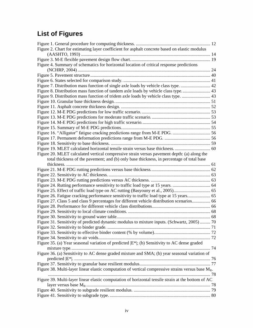
List of Figures
Figure 1. General procedure for computing thickness. ................................................................. 12 Figure 2. Chart for estimating layer coefficient for asphalt concrete based on elastic modulus
(AASHTO, 1993) ................................................................................................................. 14 Figure 3. M-E flexible pavement design flow chart. ..................................................................... 19 Figure 4. Summary of schematics for horizontal location of critical response predictions
(NCHRP, 2004) .................................................................................................................... 24 Figure 5. Pavement structure ......................................................................................................... 40 Figure 6. States selected for comparison study. ............................................................................ 41 Figure 7. Distribution mass function of single axle loads by vehicle class type. .......................... 42 Figure 8. Distribution mass function of tandem axle loads by vehicle class type. ........................ 43 Figure 9. Distribution mass function of tridem axle loads by vehicle class type. ......................... 43 Figure 10. Granular base thickness design. ................................................................................... 51 Figure 11. Asphalt concrete thickness design. .............................................................................. 52 Figure 12. M-E PDG predictions for low traffic scenario. ............................................................ 53 Figure 13. M-E PDG predictions for moderate traffic scenario. ................................................... 53 Figure 14. M-E PDG predictions for high traffic scenario. ........................................................... 54 Figure 15. Summary of M-E PDG predictions. ............................................................................. 55 Figure 16. ―Alligator‖ fatigue cracking predictions range from M-E PDG. ................................. 56 Figure 17. Permanent deformation predictions range from M-E PDG. ........................................ 56 Figure 18. Sensitivity to base thickness. ....................................................................................... 59 Figure 19. MLET calculated horizontal tensile strain versus base thickness. ............................... 60 Figure 20. MLET calculated vertical compressive strain versus pavement depth: (a) along the
total thickness of the pavement; and (b) only base thickness, in percentage of total base
thickness. .............................................................................................................................. 61 Figure 21. M-E PDG rutting predictions versus base thickness. ................................................... 62 Figure 22. Sensitivity to AC thickness. ......................................................................................... 63 Figure 23. M-E PDG rutting predictions versus AC thickness. .................................................... 63 Figure 24. Rutting performance sensitivity to traffic load type at 15 years. ................................. 64 Figure 25. Effect of traffic load type on AC rutting (Basyouny et al., 2005). ............................... 65 Figure 26. Fatigue cracking performance sensitivity to traffic load type at 15 years. ................... 65 Figure 27. Class 5 and class 9 percentages for different vehicle distribution scenarios................ 66 Figure 28. Performance for different vehicle class distributions. .................................................. 66 Figure 29. Sensitivity to local climate conditions. ........................................................................ 68 Figure 30. Sensitivity to ground water table.................................................................................. 68 Figure 31. Sensitivity of predicted dynamic modulus to mixture inputs. (Schwartz, 2005) ......... 70 Figure 32. Sensitivity to binder grade. .......................................................................................... 71 Figure 33. Sensitivity to effective binder content (% by volume). ................................................ 72 Figure 34. Sensitivity to air voids. ................................................................................................. 72 Figure 35. (a) Year seasonal variation of predicted |E*|; (b) Sensitivity to AC dense graded
mixture type. ......................................................................................................................... 74 Figure 36. (a) Sensitivity to AC dense graded mixture and SMA; (b) year seasonal variation of
predicted |E*|. ....................................................................................................................... 76 Figure 37. Sensitivity to granular base resilient modulus.............................................................. 77 Figure 38. Multi-layer linear elastic computation of vertical compressive strains versus base MR.
.............................................................................................................................................. 78 Figure 39. Multi-layer linear elastic computation of horizontal tensile strain at the bottom of AC
layer versus base MR. ............................................................................................................ 78 Figure 40. Sensitivity to subgrade resilient modulus. ................................................................... 79 Figure 41. Sensitivity to subgrade type. ........................................................................................ 80
v
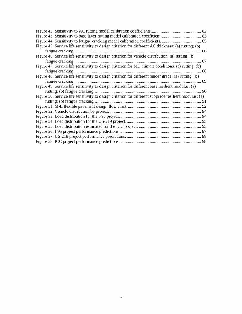
Figure 42. Sensitivity to AC rutting model calibration coefficients. ............................................. 82 Figure 43. Sensitivity to base layer rutting model calibration coefficient. .................................... 83 Figure 44. Sensitivity to fatigue cracking model calibration coefficients. .................................... 85 Figure 45. Service life sensitivity to design criterion for different AC thickness: (a) rutting; (b)
fatigue cracking. ................................................................................................................... 86 Figure 46. Service life sensitivity to design criterion for vehicle distribution: (a) rutting; (b)
fatigue cracking. ................................................................................................................... 87 Figure 47. Service life sensitivity to design criterion for MD climate conditions: (a) rutting; (b)
fatigue cracking. ................................................................................................................... 88 Figure 48. Service life sensitivity to design criterion for different binder grade: (a) rutting; (b)
fatigue cracking. ................................................................................................................... 89 Figure 49. Service life sensitivity to design criterion for different base resilient modulus: (a)
rutting; (b) fatigue cracking. ................................................................................................. 90 Figure 50. Service life sensitivity to design criterion for different subgrade resilient modulus: (a)
rutting; (b) fatigue cracking. ................................................................................................. 91 Figure 51. M-E flexible pavement design flow chart. ................................................................... 92 Figure 52. Vehicle distribution by project. .................................................................................... 94 Figure 53. Load distribution for the I-95 project. .......................................................................... 94 Figure 54. Load distribution for the US-219 project. .................................................................... 95 Figure 55. Load distribution estimated for the ICC project. ......................................................... 95 Figure 56. I-95 project performance predictions. .......................................................................... 97 Figure 57. US-219 project performance predictions. .................................................................... 98 Figure 58. ICC project performance predictions. .......................................................................... 98
1
1. Introduction
Pavement structural design is a daunting task. Although the basic geometry of a pavement system
is quite simple, everything else is not. Traffic loading is a heterogeneous mix of vehicles, axle
types, and axle loads with distributions that vary with time throughout the day, from season to
season, and over the pavement design life. Pavement materials respond to these loads in complex
ways influenced by stress state and magnitude, temperature, moisture, time, loading rate, and
other factors. Exposure to harsh environmental conditions ranging from subzero cold to blistering
heat and from parched to saturated moisture states adds further complications. It should be no
wonder, then, that the profession has resorted to largely empirical methods like the American
Association of State Highway and Transportation Officials (AASHTO) guides for pavement
design (AASHTO, 1993).
Several developments over recent decades have offered an opportunity for more rational and
rigorous pavement design procedures. Advances in computational mechanics and in the
computers available for performing the calculations have greatly improved our ability to predict
pavement response to load and climate effects. Improved material characterization and
constitutive models make it possible to incorporate nonlinearities, rate effects, and other realistic
features of material behavior. Large databases now exist for traffic characteristics, site climate
conditions, pavement material properties, and historical performance of in-service pavement
sections. These and other assets provided the technical infrastructure that made possible the
development of the mechanistic-empirical pavement design procedure in NCHRP Project 1-37A
(NCHRP, 2004).
The objectives of this study are (1) to compare flexible pavement designs and performance
between the empirical 1993 AASHTO pavement design guide and the mechanistic-empirical
pavement design guide developed in NCHRP 1-37A, hereafter termed the M-E PDG; and (2) to
perform a sensitivity analysis of the M-E PDG’s input parameters. The comparisons span a range
of locations within the United States, each with its own climate, subgrade and other material
properties, and local design preferences. Particular emphasis is devoted to the influence of traffic
and reliability levels on the comparisons. The sensitivity study is performed for several key input
variables. A design exercise consisting of three Maryland projects is presented, from which
inferences regarding appropriate design criteria for rutting and bottom-up fatigue cracking are
also drawn.
This report is divided in seven chapters. The first chapter presents an introduction, the objective
of the research, and the description of the chapters.
The second chapter is the literature review of the most relevant pavement design methods. The
methods are grouped in two categories, empirical and mechanistic-empirical, paralleling the focus
at the research objectives.
The third chapter describes the 1993 AASHTO pavement design guide and the new M-E PDG.
The fourth chapter examines differences between pavement designs in the 1993 AASHTO guide
and the M-E PDG methodologies. Typical 1993 AASHTO designs for five different regions in
the U.S. and three traffic levels are analyzed using the latest version of the M-E PDG software.
Comparisons are made based on fatigue cracking and permanent deformation predictions from
the mechanistic-empirical procedure.

2
The fifth chapter describes the results of the M-E PDG parametric sensitivity study of key inputs
and their impact on the predicted performance in terms of reasonableness and consistency with
expected field results. The sensitivity analyses are performed for fatigue cracking and permanent
deformation both in terms of the magnitudes of the predicted distresses and the impacts on
service life.
The sixth chapter presents application examples for Maryland designs obtained from the
Maryland State Highway Administration (MDSHA). Three 1993 AASHTO designs are evaluated
using the M-E PDG.
The seventh chapter presents a summary of conclusions, final remarks and recommendations for
future studies involving the application and implementation of the new mechanistic-empirical
pavement design guide.

3
2. Review of Flexible Pavement Design Principles
Before the 1920s, pavement design consisted basically of defining thicknesses of layered
materials that would provide strength and protection to a soft, weak subgrade. Pavements were
designed against subgrade shear failure. Engineers used their experience based on successes and
failures of previous projects. As experience evolved, several pavement design methods based on
subgrade shear strength were developed.
Since then, traffic volume has increased and the design criteria have changed. As important as
providing subgrade support, it was equally important to evaluate pavement performance through
ride quality and other surface distresses that increase the rate of deterioration of pavement
structures. Performance became the focus point of pavement designs. Methods based on
serviceability (an index of the pavement service quality) were developed based on test track
experiments. The AASHO Road Test in 1960s was a seminal experiment from which the
AASHTO design guide was developed.
Methods developed from laboratory test data or test track experiments in which model curves are
fitted to data are typical examples of empirical methods. Although they may exhibit good
accuracy, empirical methods are valid only for the materials and climate conditions for which
they were developed.
Meanwhile, new materials started to be used in pavement structures that provided better subgrade
protection, but with their own failure modes. New design criteria were required to incorporate
such failure mechanisms (e.g., fatigue cracking and permanent deformation in the case of asphalt
concrete). The Asphalt Institute method (Asphalt Institute, 1982, 1991) and the Shell method
(Claussen et al., 1977; Shook et al., 1982) are examples of procedures based on asphalt concrete’s
fatigue cracking and permanent deformation failure modes. These methods were the first to use
linear-elastic theory of mechanics to compute structural responses (in this case strains) in
combination with empirical models to predict number of loads to failure for flexible pavements.
The dilemma is that pavement materials do not exhibit the simple behavior assumed in isotropic
linear-elastic theory. Nonlinearities, time and temperature dependency, and anisotropy are some
examples of complicated features often observed in pavement materials. In this case, advanced
modeling is required to predict performance mechanistically. The mechanistic design approach is
based on the theories of mechanics and relates pavement structural behavior and performance to
traffic loading and environmental influences. Progress has been made in recent years on isolated
pieces of the mechanistic performance prediction problem, but the reality is that fully mechanistic
methods are not yet available for practical pavement design.
The mechanistic-empirical approach is a hybrid approach. Empirical models are used to fill in the
gaps that exist between the theory of mechanics and the performance of pavement structures.
Simple mechanistic responses are easy to compute with assumptions and simplifications (i.e.,
homogeneous material, small strain analysis, static loading as typically assumed in linear elastic
theory), but they by themselves cannot be used to predict performance directly; some type of
empirical model is required to make the appropriate correlation. Mechanistic-empirical methods
are considered an intermediate step between empirical and fully mechanistic methods.
The objective of this section is to review briefly some of these advancements in pavement design,
focusing on flexible pavements. The nomenclature in the literature often shows several groups of
different pavement design methods, mostly according to their origin and development techniques.
4
For simplification, pavement design methods in this study are grouped as empirical and
mechanistic-empirical.
2.1 Empirical Methods
An empirical design approach is one that is based solely on the results of experiments or
experience. Observations are used to establish correlations between the inputs and the outcomes
of a process--e.g., pavement design and performance. These relationships generally do not have a
firm scientific basis, although they must meet the tests of engineering reasonableness (e.g., trends
in the correct directions, correct behavior for limiting cases, etc.). Empirical approaches are often
used as an expedient when it is too difficult to define theoretically the precise cause-and-effect
relationships of a phenomenon.
The first empirical methods for flexible pavement design date to the mid-1920s when the first soil
classifications were developed. One of the first to be published was the Public Roads (PR) soil
classification system (Hogentogler & Terzaghi, 1929, after Huang, 2004). In 1929, the California
Highway Department developed a method using the California Bearing Ratio (CBR) strength test
(Porter, 1950, after Huang, 2004). The CBR method related the material’s CBR value to the
required thickness to provide protection against subgrade shear failure. The thickness computed
was defined for the standard crushed stone used in the definition of the CBR test. The CBR
method was improved by U.S. Corps of Engineers (USCE) during the World War II and later
became the most popular design method. In 1945 the Highway Research Board (HRB) modified
the PR classification. Soils were grouped in 7 categories (A-1 to A-7) with indexes to
differentiate soils within each group. The classification was applied to estimate the subbase
quality and total pavement thicknesses.
Several methods based on subgrade shear failure criteria were developed after the CBR method.
Barber (1946, after Huang 2004) used Terzaghi’s bearing capacity formula to compute pavement
thickness, while McLeod (1953, after Huang 2004) applied logarithmic spirals to determine
bearing capacity of pavements. However, with increasing traffic volume and vehicle speed, new
materials were introduced in the pavement structure to improve performance and smoothness and
shear failure was no longer the governing design criterion.
The first attempt to consider a structural response as a quantitative measure of the pavement
structural capacity was measuring surface vertical deflection. A few methods were developed
based on the theory of elasticity for soil mass. These methods estimated layer thickness based on
a limit for surface vertical deflection. The first one published was developed by the Kansas State
Highway Commission, in 1947, in which Boussinesq’s equation was used and the deflection of
subgrade was limited to 2.54 mm. Later in 1953, the U.S. Navy applied Burmister’s two-layer
elastic theory and limited the surface deflection to 6.35 mm. Other methods were developed over
the years, incorporating strength tests. More recently, resilient modulus has been used to establish
relationships between the strength and deflection limits for determining thicknesses of new
pavement structures and overlays (Preussler and Pinto, 1984). The deflection methods were most
appealing to practitioners because deflection is easy to measure in the field. However, failures in
pavements are caused by excessive stress and strain rather than deflection.
After 1950, experimental tracks started to be used for gathering pavement performance data.
Regression models were developed linking the performance data to design inputs. The empirical
AASHTO method (AASHTO, 1993), based on the AASHO Road Test from the late 1950s, is the
most widely used pavement design method today. The AASTHO design equation is a regression
relationship between the number of load cycles, pavement structural capacity, and performance,
5
measured in terms of serviceability. The concept of serviceability was introduced in the
AASHTO method as an indirect measure of the pavement’s ride quality. The serviceability index
is based on surface distresses commonly found in pavements.
The biggest disadvantage of regression methods is the limitation on their application. As is the
case for any empirical method, regression methods can be applied only to the conditions similar
to those for which they were developed. The AASHTO method, for example, has been adjusted
several times over the years to incorporate extensive modifications based on theory and
experience that allowed the design equation to be used under conditions other than those of the
AASHO Road Test.
In addition to test tracks, regression equations can also be developed using performance data from
existing pavements. Examples include the COPES (Darter et al., 1985) and EXPEAR (Hall et al.,
1989) systems. Although these models can represent and explain the effects of specific factors on
pavement performance, their limited consideration of materials and construction data result in
wide scatter and many uncertainties. Their use as pavement design tools is therefore very limited.
2.2 Mechanistic-Empirical Methods
Mechanistic-empirical (M-E) methods represent one step forward from empirical methods. The
induced state of stress and strain in a pavement structure due to traffic loading and environmental
conditions is predicted using theory of mechanics. Empirical models link these structural
responses to distress predictions. Kerkhoven & Dormon (1953) first suggested the use of vertical
compressive strain on the top of subgrade as a failure criterion to reduce permanent deformation.
Saal & Pell (1960) published the use of horizontal tensile strain at the bottom of asphalt layer to
minimize fatigue cracking. Dormon & Metcalf (1965) first used these concepts for pavement
design. The Shell method (Claussen et al., 1977) and the Asphalt Institute method (Shook et al.,
1982; AI, 1992) incorporated strain-based criteria in their mechanistic-empirical procedures.
Several studies over the past fifteen years have advanced mechanistic-empirical techniques. Most
of work, however, was based on variants of the same two strain-based criteria developed by Shell
and the Asphalt Institute. The Departments of Transportation of the Washington State (WSDOT),
North Carolina (NCDOT) and Minnesota (MNDOT), to name a few, developed their own M-E
procedures. The National Cooperative Highway Research Program (NCHRP) 1-26 project report,
Calibrated Mechanistic Structural Analysis Procedures for Pavements (1990), provided the basic
framework for most of the efforts attempted by state DOTs. WSDOT (Pierce et al., 1993;
WSDOT, 1995) and NCDOT (Corley-Lay, 1996) developed similar M-E frameworks
incorporating environmental variables (e.g., asphalt concrete temperature to determine stiffness)
and cumulative damage model using Miner’s Law with the fatigue cracking criterion. MNDOT
(Timm et al., 1998) adopted a variant of the Shell’s fatigue cracking model developed in Illinois
(Thompson, 1985) and the Asphalt Institute’s rutting model.
The NCHRP 1-37A project (NCHRP, 2004) delivered the most recent M-E-based method that
incorporates nationally calibrated models to predict distinct distresses induced by traffic load and
environmental conditions. The NCHRP 1-37A methodology also incorporates vehicle class and
load distributions in the design, a step forward from the Equivalent Single Axle Load (ESAL)
approach used in the AASTHO design equation and other methods. The performance
computation is done on a seasonal basis to incorporate the effects of climate conditions on the
behavior of materials.
The mechanistic-empirical pavement design guide (M-E PDG) developed in NCHRP 1-37A is
the main focus of this study. A complete description of its components, key elements, and use is

6
presented in Chapter 3. Chapter 3 also includes a complete review of the 1993 AASHTO Guide
and its previous versions. The comparison of the empirical 1993 AASHTO Guide and the M-E
PDG, which is one of the objectives of this study, is presented in Chapter 4.

7
3. Pavement Design Procedures
The current 1993 AASHTO Guide and the new M-E PDG for flexible pavements are described in
this chapter. The 1993 AASHTO is the latest version of AASHTO Guide for pavement design
and analysis and is a largely empirical method based primarily on the AASHO Road Test
conducted in the late 1950s. Over the years adjustments and modifications have been made in an
effort to upgrade and expand the limits over which the AASHTO guide is valid (HRB, 1962;
AASHTO, 1972, 1986, 1993).
The Federal Highway Administration’s 1995-1997 National Pavement Design Review found that
some 80 percent of states use one of the versions of the AASHTO Guide. Of the 35 states that
responded to a 1999 survey by Newcomb and Birgisson (1999), 65 percent reported using the
1993 AASHTO guide for both flexible and rigid pavement designs.
A 1996 workshop meant to develop a framework for improving the 1993 Guide recommended
instead the development of a new guide based as much as possible on mechanistic principles. The
M-E PDG developed in NHCRP 1-37A is the result of this effort. Following independent reviews
and validations that have been ongoing since its initial release in April, 2004, the M-E PDG is
expected to be adopted by AASHTO as the new national pavement design guide.
This chapter is divided in two sections. The first describes the AASHTO Guide and its revisions
since its first edition dated 1961, with the original empirical equations derived from the AASHO
Road Test, to its latest dated 19931 (HRB, 1961, 1962; AASHTO, 1972, 1986, 1993). The second
part explains in some detail the new M-E PDG procedure (NCHRP, 2004).
3.1 The 1993 AASHTO Guide
The 1993 AASHTO Guide is the latest version of the AASHTO Interim Pavement Design Guide,
originally released in 1961. The evolution of the AASHTO Guide is outlined, followed by a
description of the current design equation and input variables. At the end of this section, a
summary of recent evaluation studies of the AASHTO guide is also presented.
3.1.1 AASHO Road Test and Early Versions of the Guide
After two successful road projects, the Road Test One-MD and the WASHO Road Test (Western
Association of State Highway Officials), in 1955 the Highway Research Board (HRB) approved
the construction of a new test track project located in Ottawa, Illinois. This test facility was
opened to traffic in 1958. Traffic operated on the pavement sections until November, 1960, and a
little more than 1 million axle loads were applied to the pavement and bridges. (HRB, 1961)
The main objective of the AASHO Road Test was to determine the relation between the number
of repetitions of specified axle loads (different magnitudes and arrangements) and the
performance of different flexible and rigid pavement structures.
The test track consisted of 6 loops, each with a segment of four-lane divided highway (two lanes
per direction) whose parallel roadways were connected with a turnaround at both ends. Five loops
were trafficked and loop 1 received no traffic during the entire experiment. Test sections were
located only on tangents separated by short transition lengths. The inner and outer lanes had
1 The supplement of the 1993 AASHTO Guide, released in 1998 (AASHTO, 1998), substantially modified
the rigid pavement design procedure, based on recommendations from NCHRP Project 1-30 and studies
conducted using the LTPP database. However this supplement is not addressed in this report because it is
solely related to rigid pavements.
8
identical pavement sections. Each lane had its own assigned traffic level. The subgrade was
identified as a fine grained silty clay (A-6 or A-7-6 according to the AASHTO soil classification).
For uniformity purposes, the top 3 ft of the embankment consisted of an A-6 soil borrowed from
areas along the right-of-way of the project. The climate was temperate (average summer
temperature of 76 °F and 27 °F in winter, annual precipitation of 34 inches) with frost/thaw
cycles during the winter/spring months. (HRB, 1962)
The Concept of Serviceability and Structural Number
The performance of various pavements is a function of their relative ability to serve traffic over a
period of time. This definition of ―relative‖ performance was stated in Appendix F of the HRB
Special Report 61E that described the findings of the pavement research at the AASHO Road
Test (HRB, 1962). It goes further stating: ―At the time, there were no widely accepted definitions
of performance and therefore, a ―relative‖ performance definition should be used instead.‖
The concept of serviceability is supported by five fundamental assumptions: (1) highways are for
the comfort of the traveling user; (2) the user’s opinion as to how a highway should perform is
highly subjective; (3) there are characteristics that can be measured and related to user’s
perception of performance; (4) performance may be expressed by the mean opinion of all users;
and (5) performance is assumed to be a reflection of serviceability with increasing load
applications.
Based on these assumptions the definition of present serviceability is: ―The ability of a specific
section of pavement to serve high speed, high volume, and mixed traffic in its existing condition.‖
(HRB, 1962) The Present Serviceability Ratio (PSR) is the average of all users’ ratings of a
specific pavement section on a scale from 5 to 0 (being 5 very good and 0 very poor). The
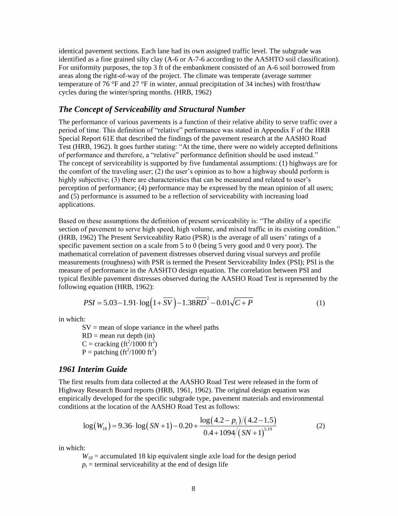
mathematical correlation of pavement distresses observed during visual surveys and profile
measurements (roughness) with PSR is termed the Present Serviceability Index (PSI); PSI is the
measure of performance in the AASHTO design equation. The correlation between PSI and
typical flexible pavement distresses observed during the AASHO Road Test is represented by the
following equation (HRB, 1962):
2
5.03 1.91 log 1 1.38 0.01PSI SV RD C P (1)
in which:
SV = mean of slope variance in the wheel paths
RD = mean rut depth (in)
C = cracking (ft2/1000 ft
2)
P = patching (ft2/1000 ft
2)
1961 Interim Guide
The first results from data collected at the AASHO Road Test were released in the form of
Highway Research Board reports (HRB, 1961, 1962). The original design equation was
empirically developed for the specific subgrade type, pavement materials and environmental
conditions at the location of the AASHO Road Test as follows:
18 5.19
log 4.2 4.2 1.5log 9.36 log 1 0.20
0.4 1094 1
tpW SN
SN
(2)
in which:
W18 = accumulated 18 kip equivalent single axle load for the design period
pt = terminal serviceability at the end of design life
9
SN = structural number
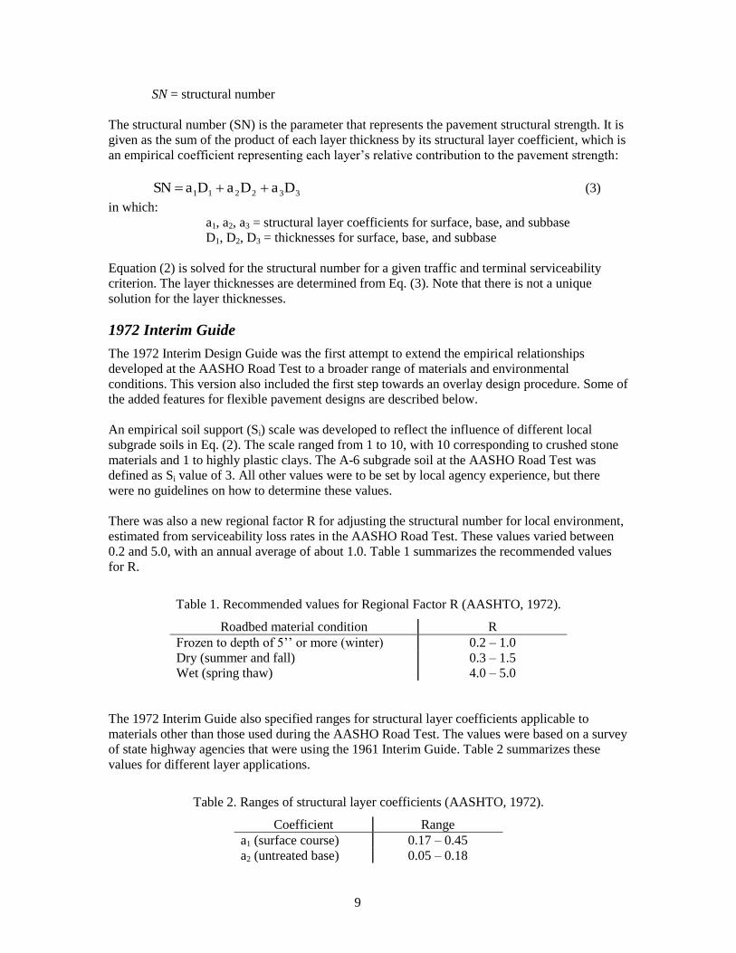
The structural number (SN) is the parameter that represents the pavement structural strength. It is
given as the sum of the product of each layer thickness by its structural layer coefficient, which is
an empirical coefficient representing each layer’s relative contribution to the pavement strength:
332211 Da Da Da SN (3)
in which:
a1, a2, a3 = structural layer coefficients for surface, base, and subbase
D1, D2, D3 = thicknesses for surface, base, and subbase
Equation (2) is solved for the structural number for a given traffic and terminal serviceability
criterion. The layer thicknesses are determined from Eq. (3). Note that there is not a unique
solution for the layer thicknesses.
1972 Interim Guide
The 1972 Interim Design Guide was the first attempt to extend the empirical relationships
developed at the AASHO Road Test to a broader range of materials and environmental
conditions. This version also included the first step towards an overlay design procedure. Some of
the added features for flexible pavement designs are described below.
An empirical soil support (Si) scale was developed to reflect the influence of different local
subgrade soils in Eq. (2). The scale ranged from 1 to 10, with 10 corresponding to crushed stone
materials and 1 to highly plastic clays. The A-6 subgrade soil at the AASHO Road Test was
defined as Si value of 3. All other values were to be set by local agency experience, but there
were no guidelines on how to determine these values.
There was also a new regional factor R for adjusting the structural number for local environment,
estimated from serviceability loss rates in the AASHO Road Test. These values varied between
0.2 and 5.0, with an annual average of about 1.0. Table 1 summarizes the recommended values
for R.
Table 1. Recommended values for Regional Factor R (AASHTO, 1972).
Roadbed material condition R
Frozen to depth of 5’’ or more (winter) 0.2 – 1.0
Dry (summer and fall) 0.3 – 1.5
Wet (spring thaw) 4.0 – 5.0
The 1972 Interim Guide also specified ranges for structural layer coefficients applicable to
materials other than those used during the AASHO Road Test. The values were based on a survey
of state highway agencies that were using the 1961 Interim Guide. Table 2 summarizes these
values for different layer applications.
Table 2. Ranges of structural layer coefficients (AASHTO, 1972).
Coefficient Range
a1 (surface course) 0.17 – 0.45
a2 (untreated base) 0.05 – 0.18
10
a3 (subbase) 0.05 – 0.14
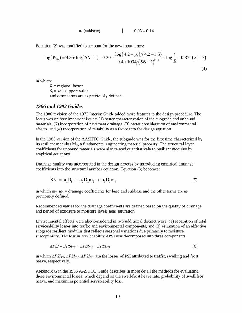
Equation (2) was modified to account for the new input terms:
18 5.19
log 4.2 4.2 1.5 1log 9.36 log 1 0.20 log 0.372 3
0.4 1094 1
t
i
pW SN S
RSN
(4)
in which:
R = regional factor
Si = soil support value
and other terms are as previously defined
1986 and 1993 Guides
The 1986 revision of the 1972 Interim Guide added more features to the design procedure. The
focus was on four important issues: (1) better characterization of the subgrade and unbound
materials, (2) incorporation of pavement drainage, (3) better consideration of environmental
effects, and (4) incorporation of reliability as a factor into the design equation.
In the 1986 version of the AASHTO Guide, the subgrade was for the first time characterized by
its resilient modulus MR, a fundamental engineering material property. The structural layer
coefficients for unbound materials were also related quantitatively to resilient modulus by
empirical equations.
Drainage quality was incorporated in the design process by introducing empirical drainage
coefficients into the structural number equation. Equation (3) becomes:
1 1 2 2 2 3 3 3SN a D a D m a D m (5)
in which m2, m3 = drainage coefficients for base and subbase and the other terms are as
previously defined.
Recommended values for the drainage coefficients are defined based on the quality of drainage
and period of exposure to moisture levels near saturation.
Environmental effects were also considered in two additional distinct ways: (1) separation of total
serviceability losses into traffic and environmental components, and (2) estimation of an effective
subgrade resilient modulus that reflects seasonal variations due primarily to moisture
susceptibility. The loss in serviceability ΔPSI was decomposed into three components:
ΔPSI = ΔPSITR + ΔPSISW + ΔPSIFH (6)
in which ΔPSITR, ΔPSISW, ΔPSIFH are the losses of PSI attributed to traffic, swelling and frost
heave, respectively.
Appendix G in the 1986 AASHTO Guide describes in more detail the methods for evaluating
these environmental losses, which depend on the swell/frost heave rate, probability of swell/frost
heave, and maximum potential serviceability loss.

11
Reliability was introduced into the 1986 AASHTO Guide to account for the effects of uncertainty
and variability in the design inputs. Although it represents the uncertainty of all inputs, it is very
simply incorporated in the design equation through factors that modify the allowable design
traffic (W18).
There were few changes to the flexible pavement design procedure between the 1986 version and
the current 1993 version. Most of the enhancements were geared towards rehabilitation, the use of
nondestructive testing for evaluation of existing pavements, and backcalculation of layer moduli
for determination of the layer coefficients. The design equation did not change from the 1986 to
1993 version. The complete description of the 1993 AASHTO Guide is presented in the
following subsections.
3.1.2 Current Design Equation
The 1993 AASHTO Guide specifies the following empirical design equation for flexible
pavements:
18 0 5.19
log 4.2 1.5log 9.36 log 1 0.20 2.32 log 8.07
0.4 1094 1R
PSIW Z S SN MR
SN
(7)
in which:
W18 = accumulated 18 kip equivalent single axle load for the design period
ZR = reliability factor
S0 = standard deviation
SN = structural number
PSI = initial PSI – terminal PSI
MR = subgrade resilient modulus (psi)
The solution of Eq. (7) follows the same procedure described before for the previous versions of
the Guide. Given all the inputs, Eq. (7) is solved for the structural number (SN) and then the layer
thicknesses can be computed. The solution is not unique and different combination of thicknesses
can be found. Additional design constraints, such as costs and constructability, must also be
considered to determine the optimal final design. The 1993 Guide recommends the top-to-bottom
procedure in which each of the upper layers is designed to provide adequate protection to the
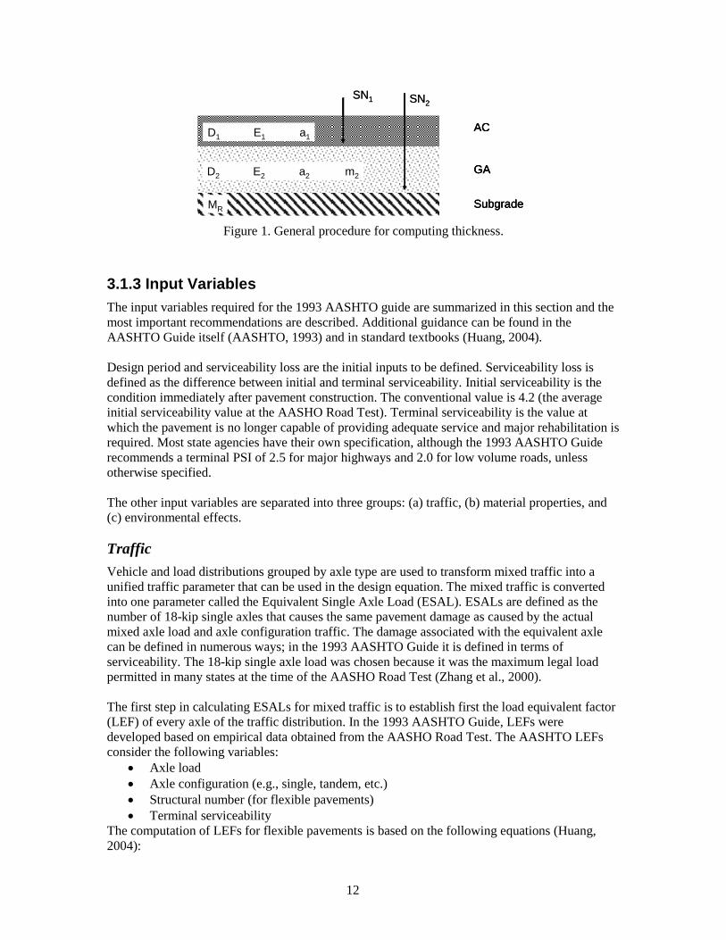
underlying layers. Figure 1 illustrates the procedure for a 3-layer flexible pavement. The steps in
this case are as follows:
Calculate SN1 required to protect the base, using E2 as MR in Eq. (7), and compute
the thickness of layer 1 as:
1
11
a
SND (8)
Calculate SN2 required to protect the subgrade, using Eq. (7), now with the subgrade
effective resilient modulus as MR. The thickness of the base is computed as:
22
1122
ma
DaSND
(9)
12
AC
GA
Subgrade
D2 E2 a2 m2
D1 E1 a1
MR
SN1 SN2
AC
GA
Subgrade
AC
GA
Subgrade
D2 E2 a2 m2
D1 E1 a1
MR
SN1 SN2
Figure 1. General procedure for computing thickness.
3.1.3 Input Variables
The input variables required for the 1993 AASHTO guide are summarized in this section and the
most important recommendations are described. Additional guidance can be found in the
AASHTO Guide itself (AASHTO, 1993) and in standard textbooks (Huang, 2004).
Design period and serviceability loss are the initial inputs to be defined. Serviceability loss is
defined as the difference between initial and terminal serviceability. Initial serviceability is the
condition immediately after pavement construction. The conventional value is 4.2 (the average
initial serviceability value at the AASHO Road Test). Terminal serviceability is the value at
which the pavement is no longer capable of providing adequate service and major rehabilitation is
required. Most state agencies have their own specification, although the 1993 AASHTO Guide
recommends a terminal PSI of 2.5 for major highways and 2.0 for low volume roads, unless
otherwise specified.
The other input variables are separated into three groups: (a) traffic, (b) material properties, and
(c) environmental effects.
Traffic
Vehicle and load distributions grouped by axle type are used to transform mixed traffic into a
unified traffic parameter that can be used in the design equation. The mixed traffic is converted
into one parameter called the Equivalent Single Axle Load (ESAL). ESALs are defined as the
number of 18-kip single axles that causes the same pavement damage as caused by the actual
mixed axle load and axle configuration traffic. The damage associated with the equivalent axle
can be defined in numerous ways; in the 1993 AASHTO Guide it is defined in terms of
serviceability. The 18-kip single axle load was chosen because it was the maximum legal load
permitted in many states at the time of the AASHO Road Test (Zhang et al., 2000).
The first step in calculating ESALs for mixed traffic is to establish first the load equivalent factor
(LEF) of every axle of the traffic distribution. In the 1993 AASHTO Guide, LEFs were
developed based on empirical data obtained from the AASHO Road Test. The AASHTO LEFs
consider the following variables:
Axle load
Axle configuration (e.g., single, tandem, etc.)
Structural number (for flexible pavements)
Terminal serviceability
The computation of LEFs for flexible pavements is based on the following equations (Huang,
2004):

13
18t
tx
WLEF
W (10)a
2 2
18 18
log 4.79log 18 1 4.79log 4.33logtx t tx
t x
W G GL L L
W
(10)b
4.2log
4.2 1.5
tt
pG
(10)c
3.23
2
5.19 3.23
2
0.0810.40
1
x
x
L L
SN L
(10)d
in which:
Wtx = number of x-axle load applications applied over the design period
Wt18 = number of equivalent 18-kip (80 kN) single axle loads over the design period
Lx = load on one single axle, or a set of tandem or tridem, in kip
L2 = axle code (1 for single axle, 2 for tandem, and 3 for tridem)
SN = structural number of the designed pavement
pt = terminal serviceability
18 = x for Lx = 18 kip and L2 = 1
With LEF calculated for every load group, the second step is to compute the truck factor Tf as
follows:
f i i
i
T p LEF A (11)
in which:
pi = percentage of repetitions for ith load group
LEFi = LEF for the ith load group (e.g., single-12kip, tandem-22kip, etc.)
A = average number of axles per truck
The number of ESALs is calculated as follows:
YLDGTTAADTESAL f 365 (12)
in which:
AADT = annual average daily traffic
T = percentage of trucks
G = growth factor
D = trucks in design direction (%)
L = trucks in design lane (%)
Y = design period
Material Properties
The fundamental material property in the 1993 AASHTO Guide is the resilient modulus. Since
the framework was constructed based upon structural layer coefficients, empirical relationships
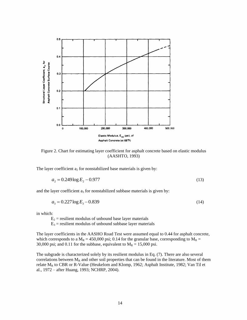
were developed to correlate resilient modulus with structural layer coefficient. Figure 2
summarizes the relationship for the layer coefficient a1 for asphalt concrete.
14
Figure 2. Chart for estimating layer coefficient for asphalt concrete based on elastic modulus
(AASHTO, 1993)
The layer coefficient a2 for nonstabilized base materials is given by:
977.0log249.0 22 Ea (13)
and the layer coefficient a3 for nonstabilized subbase materials is given by:
839.0log227.0 33 Ea (14)
in which:
E2 = resilient modulus of unbound base layer materials
E3 = resilient modulus of unbound subbase layer materials
The layer coefficients in the AASHO Road Test were assumed equal to 0.44 for asphalt concrete,
which corresponds to a MR = 450,000 psi; 0.14 for the granular base, corresponding to MR =
30,000 psi; and 0.11 for the subbase, equivalent to MR = 15,000 psi.
The subgrade is characterized solely by its resilient modulus in Eq. (7). There are also several
correlations between MR and other soil properties that can be found in the literature. Most of them
relate MR to CBR or R-Value (Heukelom and Klomp, 1962; Asphalt Institute, 1982; Van Til et
al., 1972 – after Huang, 1993; NCHRP, 2004).
15
Environmental Effects
Environmental effects (other than swelling and frost heave) are accounted for in two input
parameters in the 1993 AASHTO Guide, the seasonally-adjusted subgrade resilient modulus and
the drainage coefficient mi applied to the structural number in Eq. (5).
It is recommended that an effective subgrade resilient modulus be used to represent the effect of
seasonal variations, especially for moisture-sensitive fine-grained soils or for locations with
significant freeze-thaw cycles (AASHTO, 1993). The effective resilient modulus is the equivalent
modulus that would result in the same damage to the pavement as if seasonal modulus were used.
The relative damage ur is describe by the following empirical relationship:
32.281018.1
Rr Mu (15)
The average relative damage (uf) is computed by taking the average of ur of all seasons. The
effective subgrade resilient modulus is then given by:
431.0
3015
fR uM (16)
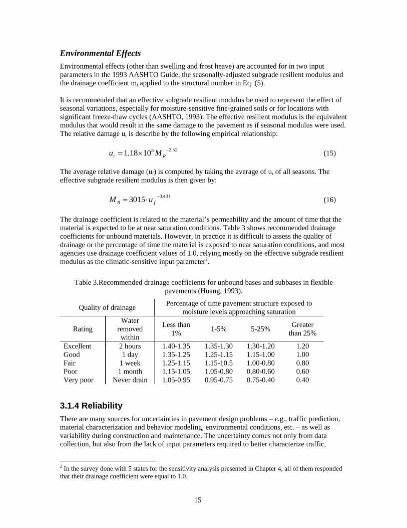
The drainage coefficient is related to the material’s permeability and the amount of time that the
material is expected to be at near saturation conditions. Table 3 shows recommended drainage
coefficients for unbound materials. However, in practice it is difficult to assess the quality of
drainage or the percentage of time the material is exposed to near saturation conditions, and most
agencies use drainage coefficient values of 1.0, relying mostly on the effective subgrade resilient
modulus as the climatic-sensitive input parameter2.
Table 3.Recommended drainage coefficients for unbound bases and subbases in flexible
pavements (Huang, 1993).
Quality of drainage Percentage of time pavement structure exposed to
moisture levels approaching saturation
Rating
Water
removed
within
Less than
1% 1-5% 5-25%
Greater
than 25%
Excellent 2 hours 1.40-1.35 1.35-1.30 1.30-1.20 1.20
Good 1 day 1.35-1.25 1.25-1.15 1.15-1.00 1.00
Fair 1 week 1.25-1.15 1.15-10.5 1.00-0.80 0.80
Poor 1 month 1.15-1.05 1.05-0.80 0.80-0.60 0.60
Very poor Never drain 1.05-0.95 0.95-0.75 0.75-0.40 0.40
3.1.4 Reliability
There are many sources for uncertainties in pavement design problems – e.g., traffic prediction,
material characterization and behavior modeling, environmental conditions, etc. – as well as
variability during construction and maintenance. The uncertainty comes not only from data
collection, but also from the lack of input parameters required to better characterize traffic,
2 In the survey done with 5 states for the sensitivity analysis presented in Chapter 4, all of them responded
that their drainage coefficient were equal to 1.0.
16
materials and environmental conditions. The reliability factor was introduced in the design
equation to account for these uncertainties.
Reliability is defined as the probability that the design pavement will achieve its design life with
serviceability higher than or equal to the specified terminal serviceability. Although the reliability
factor is applied directly to traffic in the design equation, it does not imply that traffic is the only
source of uncertainty.
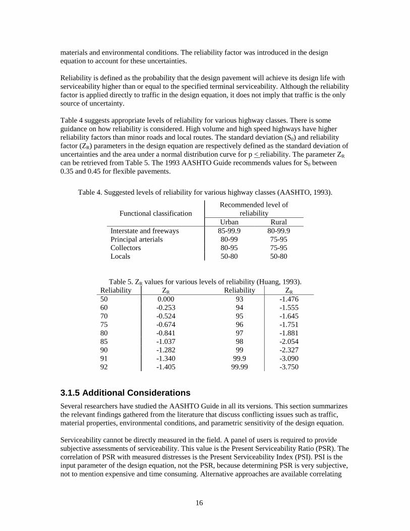
Table 4 suggests appropriate levels of reliability for various highway classes. There is some
guidance on how reliability is considered. High volume and high speed highways have higher
reliability factors than minor roads and local routes. The standard deviation (S0) and reliability
factor (ZR) parameters in the design equation are respectively defined as the standard deviation of
uncertainties and the area under a normal distribution curve for p < reliability. The parameter ZR
can be retrieved from Table 5. The 1993 AASHTO Guide recommends values for S0 between
0.35 and 0.45 for flexible pavements.
Table 4. Suggested levels of reliability for various highway classes (AASHTO, 1993).
Functional classification
Recommended level of
reliability
Urban Rural
Interstate and freeways 85-99.9 80-99.9
Principal arterials 80-99 75-95
Collectors 80-95 75-95
Locals 50-80 50-80
Table 5. ZR values for various levels of reliability (Huang, 1993).
Reliability ZR Reliability ZR
50 0.000 93 -1.476
60 -0.253 94 -1.555
70 -0.524 95 -1.645
75 -0.674 96 -1.751
80 -0.841 97 -1.881
85 -1.037 98 -2.054
90 -1.282 99 -2.327
91 -1.340 99.9 -3.090
92 -1.405 99.99 -3.750
3.1.5 Additional Considerations
Several researchers have studied the AASHTO Guide in all its versions. This section summarizes
the relevant findings gathered from the literature that discuss conflicting issues such as traffic,
material properties, environmental conditions, and parametric sensitivity of the design equation.
Serviceability cannot be directly measured in the field. A panel of users is required to provide
subjective assessments of serviceability. This value is the Present Serviceability Ratio (PSR). The
correlation of PSR with measured distresses is the Present Serviceability Index (PSI). PSI is the
input parameter of the design equation, not the PSR, because determining PSR is very subjective,
not to mention expensive and time consuming. Alternative approaches are available correlating

17
PSI with roughness, which is a more reliable, and more easily measured parameter than the
recommended distresses given in Eq. (1) (Al-Omari and Darter, 1994; Gulen et al., 1994).
Traffic has been a controversial parameter in the 1993 AASHTO Guide and its earlier versions.
The fact that it relies on a single value to represent the overall traffic spectrum is questionable.
The method used to convert the traffic spectra into ESALs by applying LEFs is also questionable.
The AASHTO LEFs consider serviceability as the damage equivalency between two axles. Zhang
et al. (2000) have found that Eq. (10), used to determine LEFs, is inconsistent with capturing
damage in terms of equivalent deflection, which is easier to measure and validate. However
quantifying damage equivalency in terms of serviceability or even deflections is not enough to
represent the complex failure modes of flexible pavements.
Several studies have been conducted to investigate effects of different load types and magnitudes
on damage of pavement structures using computed mechanistic pavement responses (Sebaaly and
Tabatabaee, 1992; Zaghloul and White, 1994). Hajek (1995) proposed a general axle load
equivalent factor – independent from pavement-related variables and axle configurations, based
only on axle load – suitable for use in pavement management systems and simple routine design
projects.
Today it is widely accepted that load equivalency factors are a simple technique for incorporating
mixed traffic into design equations and are well suited for pavement management systems.
However pavement design applications require more comprehensive procedures. Mechanistic-
empirical design procedures take a different approach for this problem; different loads and axle
geometrics are mechanistically analyzed to determine directly the most critical structural
responses that are significant to performance predictions, avoiding the shortcut of load
equivalency factors.
Layer coefficients have also been of interest to those developing and enhancing pavement design
methods. Several studies have been conducted to find layer coefficients for local and new
materials (Little, 1996; Richardson, 1996; MacGregor et al., 1999). Coree and White (1990)
presented a comprehensive analysis of layer coefficients and structural number. They showed that
the approach was not appropriate for design purposes. Baladi and Thomas (1994), through a
mechanistic evaluation of 243 pavement sections designed with the 1986 AASHTO guide,
demonstrated that the layer coefficient is not a simple function of the individual layer modulus,
but a function of all layer thicknesses and properties.
There are several studies in the literature of the environmental influences in the AASHTO
method. There are two main environmental factors that impact service life of flexible pavements:
moisture and temperature. The effect of moisture on subgrade strength has been well documented
in past years and uncountable publications about temperature effects on asphalt concrete are
available. Basma and Al-Suleiman (1991) suggested using empirical relations between moisture
content and resilient modulus directly in the design Eq. (7). The variation of the structural number
with moisture content was defined as ΔSN and was used to adjust the calculated SN. Basma and
Al-Suleiman (1991) also suggested using a nomograph containing binder and mixture properties
to determine the layer coefficient for asphalt concrete layer. Noureldin et al. (1996) developed an
approach for considering temperature effects in the 1993 AASHTO design equation. In their
approach, the mean annual pavement temperature is used to compute temperature coefficients
that modify the original asphalt concrete layer coefficient used to compute the structural number.
The 1993 AASHTO Guide and its earlier versions were developed based on results from one test
site trafficked over two years with a total of slightly over one million ESALs. From this test track,

18
which was built with the same materials varying only thicknesses, the design equation was
developed. Studies have shown that despite of the adjustments made over the years to the design
equation in attempts to expand its suitability to different climate regions and materials, the design
of flexible pavements still lacks accuracy in performance predictions and in ability to include
different materials and their complex behavior.
3.2 M-E PDG
The M-E PDG developed in NCHRP 1-37A is a mechanistic-empirical (M-E) method for
designing and evaluating pavement structures. Structural responses (stresses, strains and
deflections) are mechanistically calculated based on material properties, environmental
conditions, and loading characteristics. These responses are used as inputs in empirical models to
compute distress performance predictions. The M-E PDG was released in draft form at the
conclusion of NCHRP 1-37A in April, 2004 (NCHRP, 2004).
The M-E PDG still depends on empirical models to predict pavement performance from
calculated structural responses and material properties. The accuracy of these models is a function
of the quality of the input information and the calibration of empirical distress models to observed
field performance. Two types of empirical models are used in the M-E PDG. One type predicts
the distress directly (e.g., rutting model for flexible pavements, and faulting for rigid); the other
type predicts damage which is then calibrated against measured field distress (e.g., fatigue
cracking for flexible pavements, and punchout for rigid).
This section briefly describes the M-E PDG procedure. A description of the design process is
provided, followed by information about the components of the design procedure: inputs (design
criteria, traffic, material properties, and environmental conditions), pavement response models
(mechanistic structural computational tools and climate model), empirical performance models,
and reliability.
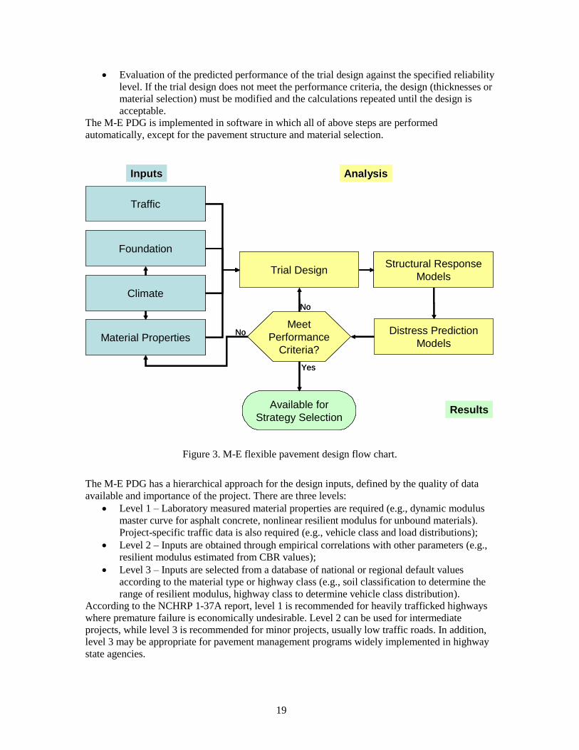
3.2.2 Design Process
The M-E PDG is not as straightforward as the 1993 AASHTO guide, in which the structure’s
thicknesses are obtained directly from the design equation. Instead an iterative process is used in
which predicted performance of selected pavement structure is compared against the design
criteria as shown in Figure 3. The structure and/or material selection are adjusted until a
satisfactory design is achieved. A step-by-step description is as follows:
Definition of a trial design for specific site subgrade support, material properties, traffic
loading, and environmental conditions;
Definition of design criteria for acceptable pavement performance at the end of the
design period (i.e., acceptable levels of rutting, fatigue cracking, thermal cracking, and
roughness);
Selection of reliability level for each one of the distresses considered in the design;
Calculation of monthly traffic loading and seasonal climate conditions (temperature
gradients in asphalt concrete layers, moisture content in unbound granular layers and
subgrade);
Modification of material properties in response to environmental conditions;
Computation of structural responses (stresses, strains and deflections) for each axle type
and load and for each time step throughout the design period;
Calculation of predicted distresses (e.g., rutting, fatigue cracking) at the end of each time
step throughout the design period using the calibrated empirical performance models;
19
Evaluation of the predicted performance of the trial design against the specified reliability
level. If the trial design does not meet the performance criteria, the design (thicknesses or
material selection) must be modified and the calculations repeated until the design is
acceptable.
The M-E PDG is implemented in software in which all of above steps are performed
automatically, except for the pavement structure and material selection.
Traffic
Foundation
Climate
Material Properties
Trial DesignStructural Response
Models
Distress Prediction
Models
Meet
Performance
Criteria?
Available for
Strategy Selection
Yes
No
No
InputsInputs AnalysisAnalysis
Results
Traffic
Foundation
Climate
Material Properties
Trial DesignStructural Response
Models
Distress Prediction
Models
Meet
Performance
Criteria?
Available for
Strategy Selection
Yes
No
No
InputsInputs AnalysisAnalysis
Results
Figure 3. M-E flexible pavement design flow chart.
The M-E PDG has a hierarchical approach for the design inputs, defined by the quality of data
available and importance of the project. There are three levels:
Level 1 – Laboratory measured material properties are required (e.g., dynamic modulus
master curve for asphalt concrete, nonlinear resilient modulus for unbound materials).
Project-specific traffic data is also required (e.g., vehicle class and load distributions);
Level 2 – Inputs are obtained through empirical correlations with other parameters (e.g.,
resilient modulus estimated from CBR values);
Level 3 – Inputs are selected from a database of national or regional default values
according to the material type or highway class (e.g., soil classification to determine the
range of resilient modulus, highway class to determine vehicle class distribution).
According to the NCHRP 1-37A report, level 1 is recommended for heavily trafficked highways
where premature failure is economically undesirable. Level 2 can be used for intermediate
projects, while level 3 is recommended for minor projects, usually low traffic roads. In addition,
level 3 may be appropriate for pavement management programs widely implemented in highway
state agencies.

20
The M-E PDG software uses the Multi Layer Linear Elastic Theory (MLET) to predict
mechanistic responses in the pavement structure. When level 1 nonlinear stiffness inputs for
unbound material are selected, MLET is not appropriate and a nonlinear Finite Element Method
(FEM) is used instead.
Level 3 was used throughout this study because (a) at present there are rarely level 1 input data to
be used on a consistent basis, and (b) the final version of the M-E PDG software was calibrated
using level 3.
3.2.3 Design Inputs
The hierarchical level defines what type of input parameter is required. This section describes the
input variables required for level 3.
Design Criteria
The design criteria are defined as the distress magnitudes at the minimum acceptable level of
service. The design criteria are agency-defined inputs that may vary by roadway class, location,
importance of the project, and economics.
The distresses considered for flexible pavements are: permanent deformation (rutting), ―alligator‖
(bottom-up) fatigue cracking, ―longitudinal‖ (top-down) cracking, thermal cracking, and
roughness. The only functional distress predicted is roughness. Friction is not considered in the
M-E PDG methodology. Among all these distresses, roughness is the only one not predicted
entirely from mechanistic responses. Roughness predictions also include other non-structural
distresses and site factors. Design criteria must be specified for each of these distresses predicted
in the M-E PDG methodology.
Traffic
The M-E PDG uses the concept of load spectra for characterizing traffic. Each axle type (e.g.,
single, tandem) is divided in a series of load ranges. Vehicle class distributions, daily traffic
volume, and axle load distributions define the number of repetitions of each axle load group at
each load level. The specific traffic inputs consist of the following data:
Traffic volume – base year information:
o Two-way annual average daily truck traffic (AADTT)
o Number of lanes in the design direction
o Percent trucks in design direction
o Percent trucks in design lane
o Vehicle (truck) operational speed
Traffic volume adjustment factors:
o Vehicle class distribution factors
o Monthly truck distribution factors
o Hourly truck distribution factors
o Traffic growth factors
Axle load distribution factors
General traffic inputs:
o Number axles/trucks
o Axle configuration
o Wheel base
o Lateral traffic wander

21
Vehicle class is defined using the FHWA classification (FHWA, 2001). Automatic Vehicle
Classification (AVC) and Weigh-in-Motion (WIM) stations can be used to provide data. The data
must be sorted by axle type and vehicle class to be used in the M-E PDG. In case site-specific
data are not available, default values are recommended in the procedure.
The use of load spectra enhances pavement design. It allows mixed traffic to be analyzed directly,
avoiding the need for load equivalency factors. Additional advantages of the load spectra
approach include: the possibility of special vehicle analyses, analysis of the impact on
performance of overloaded trucks, and analysis of weight limits during critical climate conditions
(e.g., spring thawing).
Environment
The environmental conditions are predicted by the Enhanced Integrated Climatic Model (EICM).
The following data are required:
Hourly air temperature
Hourly precipitation
Hourly wind speed
Hourly percentage sunshine
Hourly relative humidity
These parameters can be obtained from weather stations close to the project location. The M-E
PDG software includes a library of weather data for approximately 800 weather stations
throughout the U.S.
Additional environmental data are also required:
Groundwater table depth
Drainage/surface properties:
o Surface shortwave absorptivity
o Infiltration
o Drainage path length
o Cross slope
The climate inputs are used to predict moisture and temperature distributions inside the pavement
structure. Asphalt concrete stiffness is sensitive to temperature variations and unbound material
stiffness is sensitive to moisture variations. The EICM is the model is described later.
Material Properties
The M-E PDG requires a large set of material properties. Three components of the design process
require material properties: the climate model, the pavement response models, and the distress
models.
Climate-related properties are used to determine temperature and moisture variations inside the
pavement structure. The pavement response models use material properties (corrected as
appropriate for temperature and moisture effects) to compute the state of stress/strain at critical
locations in the structure due to traffic loading and temperature changes. These structural
responses are used by the distress models along with complementary material properties to
predict pavement performance.
Only flexible pavements were evaluated in this study and therefore only material properties for
asphalt concrete and unbound materials are described. Table 6 summarizes the flexible pavement
material properties required by the M-E PDG. (Recall that measured properties are level 1 inputs,
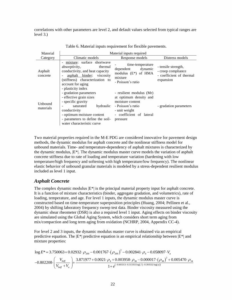
22
correlations with other parameters are level 2, and default values selected from typical ranges are
level 3.)
Table 6. Material inputs requirement for flexible pavements.
Material
Category
Material inputs required
Climatic models Response models Distress models
Asphalt
concrete
- mixture: surface shortwave
absorptivity, thermal
conductivity, and heat capacity
- asphalt binder: viscosity
(stiffness) characterization to
account for aging
- time-temperature
dependent dynamic
modulus (E*) of HMA
mixture
- Poisson’s ratio
- tensile strength,
- creep compliance
- coefficient of thermal
expansion
Unbound
materials
- plasticity index
- gradation parameters
- effective grain sizes
- specific gravity
- saturated hydraulic
conductivity
- optimum moisture content
- parameters to define the soil-
water characteristic curve
- resilient modulus (Mr)
at optimum density and
moisture content
- Poisson’s ratio
- unit weight
- coefficient of lateral
pressure
- gradation parameters
Two material properties required in the M-E PDG are considered innovative for pavement design
methods, the dynamic modulus for asphalt concrete and the nonlinear stiffness model for
unbound materials. Time- and temperature-dependency of asphalt mixtures is characterized by
the dynamic modulus, |E*|. The dynamic modulus master curve models the variation of asphalt
concrete stiffness due to rate of loading and temperature variation (hardening with low
temperature/high frequency and softening with high temperature/low frequency). The nonlinear
elastic behavior of unbound granular materials is modeled by a stress-dependent resilient modulus
included as level 1 input.
Asphalt Concrete
The complex dynamic modulus |E*| is the principal material property input for asphalt concrete.
It is a function of mixture characteristics (binder, aggregate gradation, and volumetrics), rate of
loading, temperature, and age. For level 1 inputs, the dynamic modulus master curve is
constructed based on time-temperature superposition principles (Huang, 2004; Pellinen et al.,
2004) by shifting laboratory frequency sweep test data. Binder viscosity measured using the
dynamic shear rheometer (DSR) is also a required level 1 input. Aging effects on binder viscosity
are simulated using the Global Aging System, which considers short term aging from
mix/compaction and long term aging from oxidation (NCHRP, 2004, Appendix CC-4).
For level 2 and 3 inputs, the dynamic modulus master curve is obtained via an empirical
predictive equation. The |E*| predictive equation is an empirical relationship between |E*| and
mixture properties:
2
200 200 4log * 3.750063 0.02932 0.001767 0.002841 0.058097 aE V
2
4 38 38 34
0.603313 0.313351 log 0.393532 log
3.871977 0.0021 0.003958 0.000017 0.0054700.802208
1
beff
fbeff a
V
V V e
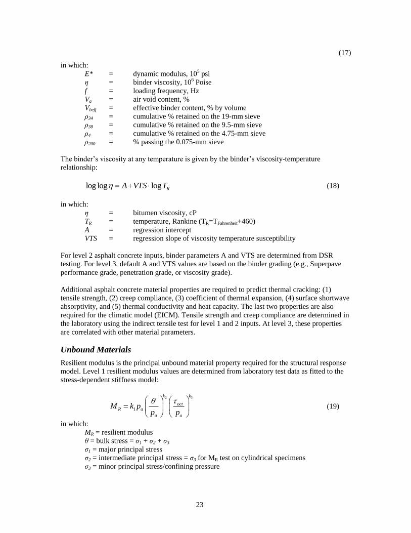
23
(17)
in which:
E* = dynamic modulus, 105 psi
η = binder viscosity, 106 Poise
f = loading frequency, Hz
Va = air void content, %
Vbeff = effective binder content, % by volume
ρ34 = cumulative % retained on the 19-mm sieve
ρ38 = cumulative % retained on the 9.5-mm sieve
ρ4 = cumulative % retained on the 4.75-mm sieve
ρ200 = % passing the 0.075-mm sieve
The binder’s viscosity at any temperature is given by the binder’s viscosity-temperature
relationship:
RTVTSA logloglog (18)
in which:
η = bitumen viscosity, cP
TR = temperature, Rankine (TR=TFahrenheit+460)
A = regression intercept
VTS = regression slope of viscosity temperature susceptibility
For level 2 asphalt concrete inputs, binder parameters A and VTS are determined from DSR
testing. For level 3, default A and VTS values are based on the binder grading (e.g., Superpave
performance grade, penetration grade, or viscosity grade).
Additional asphalt concrete material properties are required to predict thermal cracking: (1)
tensile strength, (2) creep compliance, (3) coefficient of thermal expansion, (4) surface shortwave
absorptivity, and (5) thermal conductivity and heat capacity. The last two properties are also
required for the climatic model (EICM). Tensile strength and creep compliance are determined in
the laboratory using the indirect tensile test for level 1 and 2 inputs. At level 3, these properties
are correlated with other material parameters.
Unbound Materials
Resilient modulus is the principal unbound material property required for the structural response
model. Level 1 resilient modulus values are determined from laboratory test data as fitted to the
stress-dependent stiffness model:
2 3
1
k k
octR a
a a
M k pp p
(19)
in which:
MR = resilient modulus
θ = bulk stress = σ1 + σ2 + σ3
σ1 = major principal stress
σ2 = intermediate principal stress = σ3 for MR test on cylindrical specimens
σ3 = minor principal stress/confining pressure
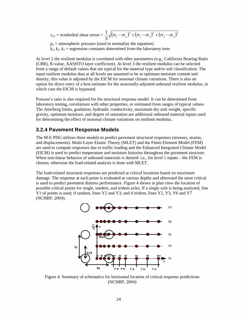
24
τoct = octahedral shear stress = 232
2
31
2
213
1
pa = atmospheric pressure (used to normalize the equation)
k1, k2, k3 = regression constants determined from the laboratory tests
At level 2 the resilient modulus is correlated with other parameters (e.g., California Bearing Ratio
(CBR), R-value, AASHTO layer coefficient). At level 3 the resilient modulus can be selected
from a range of default values that are typical for the material type and/or soil classification. The
input resilient modulus data at all levels are assumed to be at optimum moisture content and
density; this value is adjusted by the EICM for seasonal climate variations. There is also an
option for direct entry of a best estimate for the seasonally-adjusted unbound resilient modulus, in
which case the EICM is bypassed.
Poisson’s ratio is also required for the structural response model. It can be determined from
laboratory testing, correlations with other properties, or estimated from ranges of typical values.
The Atterberg limits, gradation, hydraulic conductivity, maximum dry unit weight, specific
gravity, optimum moisture, and degree of saturation are additional unbound material inputs used
for determining the effect of seasonal climate variations on resilient modulus.
3.2.4 Pavement Response Models
The M-E PDG utilizes three models to predict pavement structural responses (stresses, strains,
and displacements). Multi-Layer Elastic Theory (MLET) and the Finite Element Model (FEM)
are used to compute responses due to traffic loading and the Enhanced Integrated Climate Model
(EICM) is used to predict temperature and moisture histories throughout the pavement structure.
When non-linear behavior of unbound materials is desired–i.e., for level 1 inputs—the FEM is
chosen; otherwise the load-related analysis is done with MLET.
The load-related structural responses are predicted at critical locations based on maximum
damage. The response at each point is evaluated at various depths and afterward the most critical
is used to predict pavement distress performance. Figure 4 shows in plan view the location of
possible critical points for single, tandem, and tridem axles. If a single axle is being analyzed, line
Y1 of points is used; if tandem, lines Y2 and Y3; and if tridem, lines Y2, Y3, Y6 and Y7
(NCHRP, 2004).
Figure 4. Summary of schematics for horizontal location of critical response predictions
(NCHRP, 2004)

25
The depths at which the calculations are performed depend on the distress type:
Fatigue cracking
o at surface (top-down cracking)
o 0.5 inches from the surface (top-down cracking)
o at the bottom of the asphalt concrete layer (bottom-up cracking)
Rutting
o mid-depth of each layer/sublayer
o top of subgrade
o 6 inches below the top of subgrade
Each pavement layer is divided into thin sublayers so that properties varying in the vertical
direction are represented better (e.g., asphalt concrete layer is divided and different dynamic
moduli are assigned depending on the temperature in each sublayer). For flexible pavements, the
sublayering is determined as follows:
The first 1 inch of asphalt concrete (AC) is divided into two 0.5-inch sublayers. The
remaining AC thickness is divided into 1-inch sublayers until 4 inches of total depth from
the surface is achieved. The remaining thickness, if there is any, is considered the final
AC sublayer.
The unbound base is divided into a + nb sublayers, in which a has half the thickness of b.
The number of remaining sublayers is determined by: n=int[(hbase-2)/4]. Therefore, the
total number of sublayers is n+1. This procedure is valid for base thickness exceeding 6
inches.
The subgrade is divided into 3 sublayers of equal thickness until the total depth of the
pavement structure reaches 8 feet. From this point on there is no more sublayering and
the remaining subgrade is treated as an infinite layer.
Multi-layer Linear Elastic Theory
The first attempt to calculate displacements due to loading on an elastic half-space, such as the
surface of an homogeneous material with infinite area and depth, was made by Kelvin in 1868
(Croney and Croney, 1997). Later, Boussinesq’s solution (1885) for a concentrated load became a
fundamental tool to compute stress, strain and deflection. The solution could be integrated to
obtain responses due to a general surface load, including a circular loaded area (Huang, 1993).
The concept of multi-layer analysis has its roots in the Burmister two-layer and three-layer
solutions (Burmister, 1945); charts and tables summarizing these solutions were developed later
(Foster and Alvin, 1954; Burmister, 1958; Jones, 1962; Huang, 1969, and 1973).
Burmister’s layered theory can be applied to a multi-layer system of linear elastic materials
structured on top of a half space subgrade following the basic assumptions (Huang, 1994):
Each layer is homogeneous, isotropic, and linearly elastic, characterized by Young’s
modulus of elasticity, E, and Poisson’s ratio, ν.
The material is weightless and horizontally infinite
The thickness of each layer is finite, and the subgrade is considered as infinite layer.
The load is uniformly applied on the surface over a circular area.
Continuity conditions are satisfied at the layer interfaces.
In the M-E PDG, the MLET is implemented in a modified version of the JULEA algorithm
(NCHRP, 2004). Using the principle of superposition, single wheels can be combined spatially
into multi-wheel axles to simulate different axle configurations.

26
The small set of input parameters required by MLET facilitates its implementation and use. The
only inputs required are the layer thicknesses, the elastic properties (Young’s modulus of
elasticity and Poisson’s ratio) for each layer, the tire pressure, and the tire contact area. The main
disadvantage of MLET is its inability to consider nonlinearities often exhibited by pavement
materials.
Finite Element Method
The Finite Element Method (FEM) allows structural modeling of a multi-layer pavement section
having material properties that can vary both vertically and horizontally throughout the profile. It
is a versatile tool capable of considering three dimensional geometries, non-linear material
behavior, large strain effects, dynamic loading and other features. It is well suitable for structural
evaluation and response prediction of pavements. Although its robustness permits solving more
complex problems, the longer computational time compared to MLET represents a significant
disadvantage.
The general idea of finite element technique is the partitioning of the problem into small discrete
elements (mesh), formulating an approximation to the stress and strain variations across each
individual element, and then applying equilibrium requirements to combine the individual
elements to get the formulation for the global problem in terms of a set of simultaneous linear
equations. The solution is therefore a piecewise approximation to the true solution. In the M-E
PDG, the FEM was implemented with the following features:
Linearly elastic behavior for asphalt concrete
Nonlinearly elastic behavior (stress-dependent stiffness model) with tension cut-off for
unbound materials
Fully bonded, full slip, and intermediate interface conditions between layers
The asphalt concrete layer is modeled as a linearly elastic material with stiffness given by the
mixture dynamic modulus master curve. The stress dependence of unbound material is expressed
by the following stiffness model:
32
1
k
a
oct
k
a
aRpp
pkM
(20)
in which the parameters are as previously described. The tension cut-off feature is triggered
whenever tensile principal stresses are calculated in the unbound layers (the excess tensile stress
is distributed over neighboring elements in an iterative process). The load is applied in small
increments, and the stress/strain output from each increment provides the initial condition for the
next stage (NCHRP, Appendix RR, 2004).
EICM Environmental Model
EICM is a mechanistic model of one dimensional heat and moisture flow that simulates changes
in the behavior and characteristics of pavement and subgrade materials induced by environmental
factors (NCHRP, 2004). Daily and seasonal variations of temperature and moisture within the
pavement structure are induced by the weather history at the project site.
Different material types have different responses to climatic variations. Unbound materials are
affected by moisture change and by freeze-thaw cycles during winter and spring seasons. Asphalt
concrete responds to temperature variations, which affects directly the dynamic modulus of the
27
mixture. Temperature is also the cause of thermal cracks, either from a single thermal variation or
from repetitive cycles of warm/cool temperatures.
The EICM consists of three major components (NCHRP, 2004):
The Climatic-Materials-Structural Model (CMS Model) originally developed at the
University of Illinois (Dempsey et al., 1985)
The CRREL Frost Heave and Thaw Settlement Model (CRREL Model) originally
developed at the United States Army Cold Regions Research and Engineering Laboratory
(CRREL) (Guymon et al., 1986)
The Infiltration and Drainage Model (ID Model) originally developed at Texas A&M
University (Lytton et al., 1990)
In the case of flexible pavements, three major environmental effects are of particular interest:
Temperature variations for the asphalt concrete. The dynamic modulus of asphalt
concrete mixtures is very sensitive to temperature. Temperature distributions in asphalt
concrete layers are predicted and then used to define the stiffness of the mixture
throughout the sublayers. Temperature distributions are also used as inputs for the
thermal cracking prediction model.
Moisture variation for subgrade and unbound materials. The resilient modulus input of
unbound materials is defined as being at optimum density and moisture content. A
correction factor is defined to adjust the resilient modulus based on predicted moisture
content.
Freezing and thawing for subgrade and unbound materials. The resilient modulus of
unbound materials located within the freezing zone increases during freezing periods and
decrease during thawing periods. The EICM predicts the formation of ice lenses and
defines the freezing zone.
3.2.5 Empirical Performance Models
This section presents a description of empirical models for predicting performance of flexible
pavements in the M-E PDG. The models described here are the following: ―alligator‖ or bottom-
up fatigue cracking, longitudinal or top down fatigue cracking, thermal cracking, rutting and
roughness. The calibration of these models was done using the Long Term Pavement
Performance (LTPP) database with sections distributed all over the U.S. This calibration effort is
defined in the M-E PDG as the national calibration.
The national calibration was a task undertaken by the NCHRP 1-37A project team to determine
calibration coefficients for the empirical distress models that would be representative of the wide
range of materials available in the U.S. for pavement construction. The LTPP database was used
as primary source of data for this purpose. Permanent deformation, longitudinal (top-down),
alligator (bottom-up) and thermal cracking were calibrated for flexible pavement sections.
According to the NCHRP 1-37A report, the roughness model was developed directly using the
LTPP data and therefore required no additional calibration.
The importance of calibration is evident. Pavement structures behave in different ways and the
current state-of-the-art mechanistic models are not capable of fully predicting the behavior of
pavement structures. The empirical models are not sufficient to stand alone and capture the wide
possibilities of failure mechanism. In addition, most of these models were developed from
laboratory test data and laboratory-field shifting factors are required.

28
Alligator Fatigue Cracking
―Alligator‖ fatigue cracking develops from mechanical failure caused by tensile strains at the
bottom of asphalt concrete layers and once developed propagates upwards. It is also known as
bottom-up cracking. Stiffer mixtures or thin layers are more likely to exhibit bottom-up fatigue
cracking problems, which makes it a problem often aggravated by cold weather. It is also noted
that the supporting layers are important for the development of fatigue cracking. Soft layers
placed immediately below the asphalt concrete layer increase the tensile strain magnitude at the
bottom of the asphalt concrete and consequently increase the probability of fatigue crack
development.
Fatigue cracking is evaluated by first predicting damage and then converting damage into cracked
area. The model used in the M-E PDG was adopted from the Asphalt Institute (Asphalt Institute,
1991) and calibrated based on 82 LTPP section data in 24 states across the country (NCHRP,
2004). The number of repetitions to failure for a given load magnitude is computed as follows:
2 2 3 3
1 1
k k
f t tN k k C E
(21)
in which:
Nf = number of repetitions of a given load to failure
kt = thickness correction factor
1, 2, 3 = field calibration coefficients
k1, k2, k3 = material properties determined from regression analysis laboratory test data
C = laboratory to field adjustment factor
t = tensile strain at the critical location within asphalt concrete layer
E = asphalt concrete stiffness at given temperature
The calibration of the model using the LTPP database resulted in the following values: k1 =
0.00432, k2 = 3.9492, k3 = 1.281. The i field calibrations coefficients were assumed to be equal
to 1 for this calibration. This set of calibration coefficients is referred to in the M-E PDG as the
national calibration.
The thickness correction factor is determined as follows:
AC(11.02-3.49*h )
1
0.0036020.000398
1 e
tk
(22)
in which hAC = total AC thickness. The laboratory-field adjustment factor is given by:
10MC (23)a
4.84 0.69beff
a beff
VM
V V
(23)b
in which:
Vbeff = effective binder content (% of volume)
Va = air voids (%)
29
The damage resulted from a given load is then computed from the number of repetitions using
Miner’s Law:
1
Ti
i fi
nD
N
(24)
in which:
D = damage
T = total number of seasonal periods
ni = actual traffic for period i
Nfi = traffic repetitions of a given load to cause failure at period i
The last step is to convert damage into cracked area as follows:
1 1 2 2
4
' 'log 100
1
601C C C C D
CFC
e
(25)a
2.856
2 ' 2.40874 39.748 1 ACC h
(25)b
' '
1 22C C (25)c
in which:
FC = ―alligator‖ fatigue cracking (% of lane area)
C1, C2, C4 = constants
D = damage
hAC = total AC thickness
The calibration using the LTPP database resulted in the following values for the regression
constants: C1 = 1, C2 = 1 and C4 = 6000. Equation (25)a is of a convenient sigmoidal form that
models the two end-conditions of the damage-cracked area relationship. At 0% damage the
percentage of cracked area is equal to zero. At the other end, at 100% damage, an assumption was
adopted that only half of the area would be cracked. Therefore when damage is 100%, cracked
area is equal to 50% or 3000 ft2 over a 500 ft lane length (the total lane area considered in the M-
E PDG is 12 ft x 500 ft = 6000 ft2). The statistics for the ―alligator‖ fatigue cracking model after
calibration using 461 observations from the LTPP database standard error (Se) = 6.2%, and Se/Sy
= 0.947.
Longitudinal Cracking
Longitudinal cracking develops at the surface and propagates downward (top-down cracking).
Longitudinal crack formation in flexible pavements is conceptually similar to ―alligator‖ fatigue
cracking. Tensile strains at the top of the surface asphalt concrete layer induced by traffic loading
cause the appearance of cracks.
The M-E PDG model for longitudinal cracking follows the same formulation as for alligator
cracking. The difference is in the damage-crack relationship. Equation (21) is used to calculate
the number of applications to failure for a given load. Damage is computed using Miner’s Law,
Eq. (24). Cracking, in units of foot/mile, is then given by:
30
1 2
4
log 10010.56
1C C D
CFC
e
(26)
in which:
FC = longitudinal cracking (foot/mile)
C1, C2, C4 = calibration coefficients
D = damage
The calibration using the LTPP database resulted in the following values for the regression
constants: C1 = 7, C2 = 3.5 and C4 = 1000. The sigmoidal form model was used to model the
damage-crack length relationship. The two end-conditions are satisfied. At 0% damage the model
predicts no cracking, and at 100% damage, 500 ft of longitudinal cracking per 500 ft of pavement
(assumed only 50% of the lane with cracks on both wheel paths: 2 x 250 ft). The statistics for the
longitudinal cracking calibration based on 414 field measurements are Se = 1242.25 feet/mile and
Se/Sy = 0.977.
Thermal Cracking
Thermal cracking is a consequence of heating/cooling cycles occurring in the asphalt concrete.
The pavement surface cools down faster and with more intensity than the core of the pavement
structure, which causes thermal cracking to occur at the surface of flexible pavements. Thermal
cracks extend in the transverse direction across the full width of the pavement.
The thermal cracking model used in the M-E PDG is an enhanced version of the TCMODEL
developed under the SHRP A-005 research contract. This model has a robust theoretical
background and is the most fully mechanistic of the distress prediction components in the M-E
PDG.
The main improvement from the SHRP A-005 model was the incorporation of an advanced
analysis technique to convert data directly from the Superpave Indirect Tensile Test into
viscoelastic properties, specifically the creep compliance function that is further converted to the
relaxation modulus. The relaxation modulus is coupled with the temperature data from the EICM
to predict thermal stresses. The growth behavior of the thermal crack is calculated from the
thermal stresses.
The crack propagation is computed using Paris’s law:
nC A K (27)
in which:
ΔC = change in crack depth for each thermal cycle
ΔK = change in stress intensity factor during thermal cycle
A, n = fracture parameters for the asphalt concrete mixture
The master creep compliance function is expressed as a power law:
0 1
mD D D (28)
in which:

31
ξ = reduced time
D0, D1, m = compliance coefficients
Given the compliance function model expressed by Eq. (28), the values of n and A can be
calculated as follows:
10.8 1n
m
(29)
4.389 2.52 log10 mE n
A
(30)
in which:
m = power coefficient in the compliance function
= calibration coefficient
E = mixture stiffness
σm = undamaged mixture tensile strength
The calibration of Eq. (30) depends upon knowing the creep compliance function from indirect
tensile testing. For level 1 and 2 inputs laboratory data are required (creep compliance and tensile
strength) and for level 3 input a set of correlation equations are used to predict the creep
compliance function from mixture properties (NCHRP, 2004, Appendix HH). The calibration
coefficient β varied with the input level: 5 (level 1), 1.5 (level 2), and 3 (level 3).
The length of thermal cracking is then predicted based on an assumed relationship between the
crack depth and percentage of cracking in the pavement:
ac
f
hCNC
log1 (31)
in which:
Cf = predicted thermal cracking, ft/500ft
1 = field calibration coefficient
N( ) = standard normal distribution at ( )
C = crack depth
σ = standard deviation of the log of crack depth
hac = asphalt concrete thickness
The calibration of the thermal cracking model was based on data from the LTPP database, the
Canadian C-SHRP program, MnROAD, and one section in Peoria, IL. The value of the
calibration coefficient 1 was found equal to 400.
Rutting
Permanent deformation or rutting is a load-related distress caused by cumulative applications of
loads at moderate to high temperatures, when the asphalt concrete mixture has the lowest
stiffness. It can be divided into 3 stages. Primary rutting develops early in the service life and it is
caused predominantly by densification of the mixture (compaction effort by passing traffic) and
with decreasing rate of plastic deformations. In the secondary stage, rutting increments are
smaller at a constant rate, and the mixture is mostly undergoing plastic shear deformations. The
tertiary stage is when shear failure occurs, and the mixture flows to rupture. Usually the tertiary
32
stage is not reached in in-service pavements – preventive maintenance and rehabilitation are
required by agencies long before this stage is achieved.
Permanent deformation is predicted using empirical models. Only primary and secondary stages
are modeled. For asphalt concrete materials the model is an enhanced version of Leahy’s model
(Leahy, 1989), modified by Ayres (1997) and then by Kaloush (2001). The model for unbound
materials is based on Tseng and Lytton’s model (Tseng and Lytton, 1989), which was modified
by Ayres and later on by El-Basyouny and Witczak (NCHRP, 2004).
Total permanent deformation is the summation of rut depths from all layers:
subgradeBaseACtotal RD RD RD RD (32)
Asphalt Concrete Model
The asphalt concrete layer is subdivided into sublayers and the total predicted rut depth for the
layer is given by:
N
i
iipAC hRD1
(33)
in which:
RDAC = rut depth at the asphalt concrete layer
N = number of sublayers
(p)i = vertical plastic strain at mid-thickness of layer i
Δhi = thickness of sublayer i
The vertical plastic strain (p) at each sublayer is calculated as:
3 31 2 2
3 110p kk k
r
T N
(34)
in which:
r = computed vertical resilient strain at mid-thickness of sublayer i
σ3 = depth correction factor
k1, k2, k3 = regression coefficients derived from laboratory testing
1, 2, 3 = field calibration coefficients
T = temperature
N = number of repetitions for a given load
The depth correction factor is a function of asphalt layer thickness and depth to computational
point (mid-thickness of sublayer i) that adjusts the computed plastic strain for the confining
pressure at different depths. The depth correction factor is computed as follows:
3 1 2( ) 0.328196depthC C depth (35)a
2
1 0.1039 2.4868 17.342AC ACC h h (35)b
2
2 0.0172 1.7331 27.428AC ACC h h (35)c

33
in which:
depth = depth to the point of strain calculation
hAC = thickness of the asphalt layer
After the calibration using the national LTPP database, the regression coefficients are k1 = -
3.4488, k2 = 1.5606, k3 = 0.4791, and the assumed βi’s are equal to 1. A total of 387 observed rut
points from the 88 LTPP sections were used in the calibration effort. The goodness-of-fit
statistics for the calibration are R2 = 0.643, standard error Se = 0.055 in for the wide range
mixture types in the LTPP calibration sections.
Unbound Materials
The M-E PDG divides all unbound granular materials into sublayers, and the total rutting for each
layer is the summation of the permanent deformation of all sublayers. The permanent deformation
at any given sublayer is computed as:
iv
N
r
i hek
0
11 (36)
in which:
i = permanent deformation for sublayer i
1 = field calibration coefficient
k1 = regression coefficient determined form laboratory permanent deformation test data
0/r, , ρ = material properties
N = number of repetitions of a given load
v = computed vertical resilient strain at mid-thickness of sublayer i for a given load
hi = thickness of sublayer i
The model described in Eq. (36) is a modification of the original Tseng and Lytton’s model
(Tseng and Lytton, 1989). The material properties 0/r, , ρ are derived from other properties
according to the following relationships:
log 0.61119 0.017638 cW (37)a
7( ) 18 3.52 ( 10 ) 0.5
0
1.094 10 0.0316log
2
r r
r
e E e E
(37)b
1
7
710
1 (10 )
oC
(37)c
in which:
Wc = water content (%)
Er = resilient modulus of the layer/sublayer, psi
The parameter Co is determined by:

34
-18 3.52
0.5
(1.094 10 )ln
(0.0316 )
ro
r
EC
E
(38)
The water content can be empirically related to the ground water table depth and the resilient
modulus:
0.11920.3586*
1
0.64
51.7122555
GWT
rc
EW
(39)
The subgrade is modeled as a semi-infinite layer in the structural response models (MLET or
FEM). An adjustment on the permanent deformation models is therefore required for computing
the plastic strains in a semi-infinite layer. The plastic strain at different depths in the subgrade can
be computed by:
0( ) ( ) z
p pz e (40)
in which:
p(z) = plastic vertical strain at depth z (measured from the top of the subgrade)
p0 = plastic vertical strain at the top of the subgrade (z = 0)
z = depth measured from the top of the subgrade
α = regression coefficient
In Eq. (36), plastic strain is given by the term δi/hi. Given two points in the subgrade (the M-E
PDG procedure uses top of subgrade, z=0, and z=6 inches below the top), plastic strains are
computed and the regression coefficient α is determined from Eq. (40). The total subgrade
permanent deformation then is computed by integrating Eq. (40) over the depth of subgrade until
bedrock:
z
p0 p0
0
1
bedrock bedrockh h
SG
ee dz
k
(41)
in which, hbedrock = depth to bedrock, and the other terms are as defined previously.
A total of 88 LTPP sections were used for calibration of the permanent deformation model for
unbound materials for both base/subbase and subgrade. The regression coefficient k1 for
base/subbase and subgrade are respectively 1.673 and 1.35. The goodness-of-fit statistics are R2 =
0.62 and Se = 0.014 in for the base/subbase model, and R2 = 0.19 and Se = 0.056 in for the
subgrade model.
Roughness
Roughness is generally acknowledged as the distress most representative of the overall
serviceability of a pavement section. A rough pavement directly affects the ride quality. Any
incremental increase in surface distress causes surface roughness to increase (NCHRP, 2004).
The NCHRP 1-37A project found that permanent deformations, thermal cracking, and fatigue
cracking were the most dominant distresses affecting roughness. It was also noted that local
environmental conditions and the base type supporting the surface layer were also important

35
factors. The calibration effort considered over 350 sections having good quality data in the LTPP
database. Three models were developed for flexible pavements with different base layers:
granular base, asphalt-treated base, and cement-stabilized base. The roughness model for
conventional flexible pavements with granular base, is as follows:
200 0.0463 1 0.00119 0.1834 0.00736 0.00115
age
L RDIRI IRI SF e TC COV BC LC
(42)
in which:
IRIo = initial IRI expected within six months after construction, m/km
SF = site factor
TCL = total length of transverse cracks, m/km
COVRD = rut depth coefficient of variation, %
FCT = total area of fatigue cracking, percent of total lane area
BCT = total area of block cracking, percent of total lane area
LC = length of sealed longitudinal cracks outside the wheel path, m/km
Age = age after construction, years
The flexible pavement roughness models for the other base types have a similar form. The
structural distresses required as inputs for the roughness model are obtained from the predictions
made with the distress models discussed previously. The site factor (SF) is given by:
10
1ln11ln
102
1 02.0
4
075.0 mSD RPFI
x
PIPRSF (43)
in which:
RSD = standard deviation in the monthly rainfall, mm
Rm = average annual rainfall, mm
P0.075 = percent passing the 0.075 mm sieve
P0.02 = percent passing thee 0.02 mm sieve
PI = plasticity index
FI = average annual freezing index
The LTPP sections used for calibration provided 353 data points for this model. The goodness-of-
fit statistics are R2 = 0.62 and standard error Se = 0.387 m/km (NCHRP, 2004).
3.2.6 Reliability
Pavement design inputs have large uncertainties. The design is often based on the mean values of
the input parameters. In the M-E PDG, the key outcomes are the individual distresses, considered
as the random variables of interest. The distress distribution is considered to be normal with a
mean predicted value and a corresponding standard deviation. The standard deviation of the
distribution is estimated based on the model’s calibration error. The predicted distress considering
reliability is given by the general formulation:
reliability mean D RD D S z (44)
36
in which Dreliability is the distress prediction with reliability, Dmean is the mean distress value from
the performance model, SD is the computed standard deviation for the distress type (D), and zR is
the standard normal deviate from the normal distribution for the level of reliability selected.
The formulation in Eq. (44) for the M-E PDG models reliability in the same way as the general
reliability factor in the 1993 AASHTO Guide. Recall in the 1993 AASHTO Guide, reliability is
included in the design equation via the product of the overall standard deviation and the reliability
factor (S0 x zR).
The estimates of error are obtained from the calibration (predicted versus measured data). They
include a combined input variability from the input uncertainties, construction variability, and
model error. Therefore, the model’s error becomes a key factor in the reliability – the smaller the
error, the smaller is the gap between a design with a reliability factor (higher than 50%) and one
at the mean value (reliability = 50%).
Based on the national calibration results, the default standard error (Se) for permanent
deformations is defined for each individual layer as follows:
0.45790.1587AC ACSe RD (45)a
0.53030.1169GB GBSe RD (45)b
0.55160.1724SG SGSe RD (45)c
in which AC represents asphalt concrete, GB, granular base, and SG, subgrade. RD is the rut
depth at any given sublayer.
The standard error for alligator and longitudinal cracking are defined as follows:
1.308 2.949 log0.5 12 1 D
alligatorSe e (46)a
1.072 2.1654 log200 2300 1 D
longitudinalSe e (46)b
in which D is damage computed as the primary variable in the cracking model.
There were data available for all three input levels for the calibration of the mechanistic thermal
cracking model. Standard error equations were developed for each input level as follows:
Level 1: 1 0.2474 10.619thermal thermalSe C (47)a
Level 2: 2 0.3371 14.468thermal thermalSe C (47)b
Level 3: 3 0.6803 29.197thermal thermalSe C (47)c
It is important to notice in Eq. (47) the reduction in error estimate as input level goes from 3 to 1.
Level 1 input requires more laboratory data to better characterize the material behavior which in
turn reduces the predicted standard error.
3.2.7 Remarks
The M-E approach for designing and evaluating flexible pavements represents a major step
forward from purely empirical methods. Mechanistic models are employed for predicting
pavement responses and climatic effects on material behavior. The pavement distresses are too

37
complex to be modeled by mechanistic models only. Empirical models are employed to overcome
these limitations of theory; the empirical models establish a connection between structural
responses and performance prediction. Calibration of the empirical distress models is a critical
requirement for quality performance predictions.
38
4. Comparative Study: 1993 AASHTO vs. M-E PDG
The advent of M-E pavement performance modeling allows more realistic features to be included
in pavement analysis and design. Improvements in traffic and material characterization are among
the more important of these enhanced features. Although most of those enhancements have been
available as research-oriented design and evaluation tools in the past, routine design is still done
using empirical methods, the state-of-practice followed by most agencies.
The benefits of M-E procedures require engineers to improve the design process in several key
areas ranging from data collection to interpretation of results. Additional effort and resources
must be expended to better characterize materials, improve traffic data quality, and effectively
use environmental conditions. Implementation is also a costly, time consuming task that agencies
must be willing to undertake. Initial studies are necessary to evaluate the benefits of M-E versus
empirical design and to help agencies assess the sensitivity of M-E approach to their local
conditions. Although these studies alone are insufficient for justifying the investments required
for an agency to implement a new pavement design process, they nevertheless are an essential
first step of an implementation process.
The objectives of the sensitivity analysis in this study are as follows: (1) to compare pavement
designs using the empirical 1993 AASHTO guide and those using the M-E PDG; and (2) to
evaluate the sensitivity of pavement design and performance to each of the parameters required
by the M-E PDG. The first objective is subject of this Chapter. The second objective is reported
in Chapter 5 and is intended not only to provide a better understanding of the M-E PDG and its
nuances but also to provide information on research needs for local implementation and
calibration.
Three pavement design case studies are also presented in Chapter 6. In these case studies, designs
done with the 1993 AASHTO Guide were evaluated with the M-E PDG for different performance
criteria. The results were analyzed in the context of design limits, required pavement structure,
and service life.
4.1 Conceptual Differences: 1993 AASHTO vs. M-E PDG
The comparison between the 1993 AASHTO Guide and the M-E PDG is an important step to
understand the differences between the two approaches. As mentioned before, the key conceptual
differences can be summarized as follows:
The 1993 AASHTO guide designs pavements to a single performance criterion, the
present serviceability index (PSI), while the M-E PDG simultaneously considers multiple
performance criteria (e.g., rutting, cracking, and roughness – for flexible pavements).
The 1993 AASHTO guide directly computes the layer thicknesses. The M-E PDG is an
iterative procedure. A trial section is defined and evaluated by its predicted performance
against the design criteria. If the result is not satisfactory, the section is modified and
reanalyzed until an acceptable design is reached.
The M-E PDG requires more input parameters, especially environmental and material
properties. It also employs a hierarchical concept in which one may choose different
quality levels of input parameters depending upon the level of information and resources
available, technical issues, and the importance of the project.
The 1993 AASHTO guide was developed based on limited field test data from only one
location (Ottawa, IL). The seasonally adjusted subgrade resilient modulus and the layer
drainage coefficients are the only variables that account to some extent for environmental
39
conditions. The M-E PDG utilizes a set of project-specific climate data (air temperature,
precipitation, wind speed, relative humidity, etc.) to adjust material properties for
temperature and moisture influences.
The 1993 AASHTO guide uses the concept of ESALs to define traffic levels, while the
M-E PDG adopts the more detailed load spectra concept. Pavement materials respond
differently to traffic pattern, frequency and loading. Traffic loading in different seasons
of the year also has different effects on the response of the pavement structure. These
factors can be most effectively considered using the load spectra concept.
Although these differences seem clear, their impacts on performance prediction are more obscure.
The different ways that the two procedures define performance makes direct comparisons
difficult. The 1993 AASHTO guide predicts pavement condition as a function of distresses
translated into one single index (PSI). The M-E PDG predicts directly the structural distresses
observed in the pavement section and the PSI concept is no longer employed.
PSI was based originally on subjective assessment of pavement condition by a road testing panel.
The pavement quality rating is based on distresses observed on the pavement surface. The PSI
equation developed in the AASHO Road Test correlates PSI with the individual distresses of
slope variance (roughness), cracking and patching. The strongest correlation is with roughness,
the performance measure most closely linked to road users’ perception of pavement ride quality.
However the conditions in the AASHO Road Test in the early 1960’s (e.g., traffic volume,
vehicle characteristics, travel speeds, materials) were quite different from the conditions in
highways today. Users’ perceptions of serviceability may also have changed throughout these
years, possibly demanding better quality with continuous improvements in highway and vehicle
standards. Therefore, converting pavement distresses into serviceability for comparison purposes
is unlikely to produce useful results.
Another area that requires careful attention when making comparisons between the two
approaches is traffic data. As mentioned before, the M-E PDG does not use ESALs to define
traffic. Instead, traffic is defined by vehicle class and load distributions in terms of traffic load
spectra. In the M-E PDG each load application is analyzed individually to compute pavement
responses. These responses are used to predict distresses and damage increments that are
accumulated over load applications and time.
For these and other reasons, the comparison of results from the two design approaches seems
incompatible. The option chosen here to overcome this problem was to design pavement
structures (thicknesses) using the 1993 AASHTO guide and then analyze their predicted
performance using the M-E PDG. Using the predicted performance from the M-E PDG as the
basis for comparison assumes implicitly that the M-E PDG predictions are closer to ―correct‖
values. Given this assumption, if the 1993 AASHTO guide predicts performance correctly, then
the M-E PDG predictions of distresses for pavements designed using the 1993 AASHTO guide
should also be consistent, regardless of location of the project or traffic conditions.
In summary, the method of comparison employed in this study followed the following sequence:
(1) pavements were designed using the 1993 AASHTO guide; (2) performance of the pavement
sections were then evaluated using the M-E PDG software; (3) performance results were grouped
by traffic level and location, and compared. The main purpose of grouping is to identify trends in
performance behavior for different traffic levels and environmental conditions.
The main focus of this study was evaluation of permanent deformation and classical bottom-up or
―alligator‖ fatigue cracking. Thermal cracking, top-down longitudinal cracking, and roughness
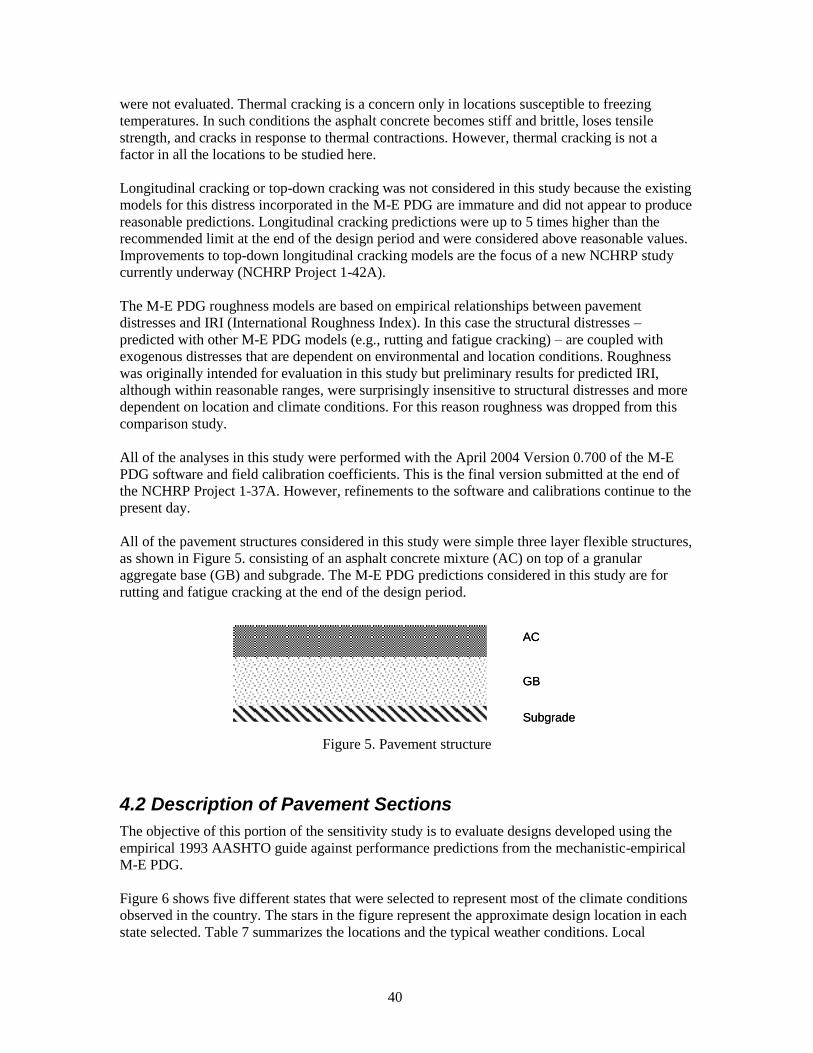
40
were not evaluated. Thermal cracking is a concern only in locations susceptible to freezing
temperatures. In such conditions the asphalt concrete becomes stiff and brittle, loses tensile
strength, and cracks in response to thermal contractions. However, thermal cracking is not a
factor in all the locations to be studied here.
Longitudinal cracking or top-down cracking was not considered in this study because the existing
models for this distress incorporated in the M-E PDG are immature and did not appear to produce
reasonable predictions. Longitudinal cracking predictions were up to 5 times higher than the
recommended limit at the end of the design period and were considered above reasonable values.
Improvements to top-down longitudinal cracking models are the focus of a new NCHRP study
currently underway (NCHRP Project 1-42A).
The M-E PDG roughness models are based on empirical relationships between pavement
distresses and IRI (International Roughness Index). In this case the structural distresses –
predicted with other M-E PDG models (e.g., rutting and fatigue cracking) – are coupled with
exogenous distresses that are dependent on environmental and location conditions. Roughness
was originally intended for evaluation in this study but preliminary results for predicted IRI,
although within reasonable ranges, were surprisingly insensitive to structural distresses and more
dependent on location and climate conditions. For this reason roughness was dropped from this
comparison study.
All of the analyses in this study were performed with the April 2004 Version 0.700 of the M-E
PDG software and field calibration coefficients. This is the final version submitted at the end of
the NCHRP Project 1-37A. However, refinements to the software and calibrations continue to the
present day.
All of the pavement structures considered in this study were simple three layer flexible structures,
as shown in Figure 5. consisting of an asphalt concrete mixture (AC) on top of a granular
aggregate base (GB) and subgrade. The M-E PDG predictions considered in this study are for
rutting and fatigue cracking at the end of the design period.
AC
GB
Subgrade
AC
GB
Subgrade
Figure 5. Pavement structure
4.2 Description of Pavement Sections
The objective of this portion of the sensitivity study is to evaluate designs developed using the
empirical 1993 AASHTO guide against performance predictions from the mechanistic-empirical
M-E PDG.
Figure 6 shows five different states that were selected to represent most of the climate conditions
observed in the country. The stars in the figure represent the approximate design location in each
state selected. Table 7 summarizes the locations and the typical weather conditions. Local
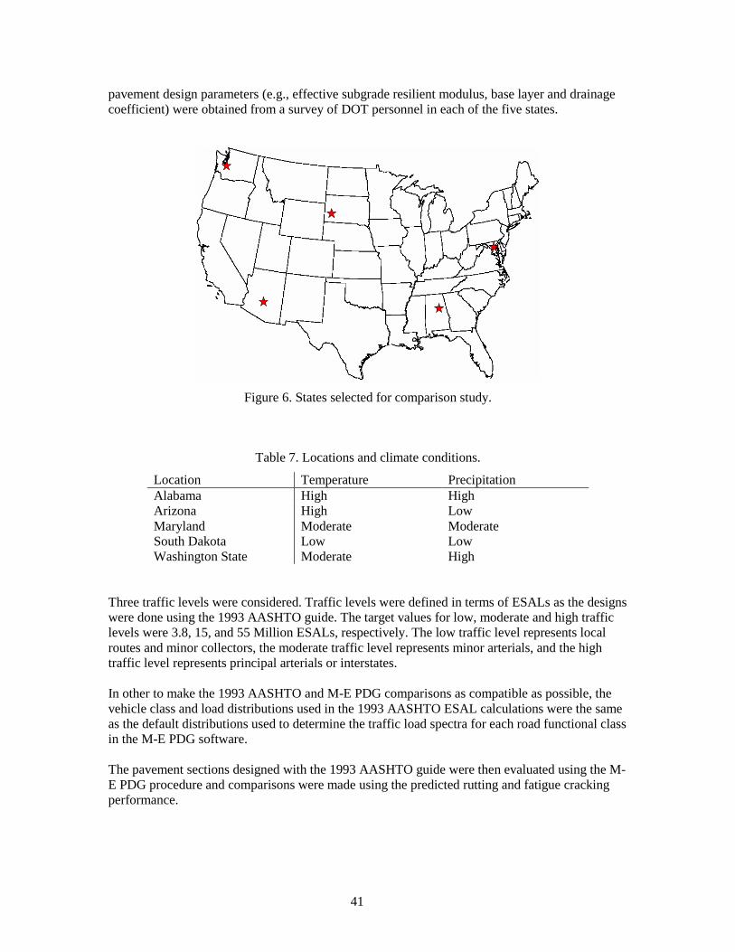
41
pavement design parameters (e.g., effective subgrade resilient modulus, base layer and drainage
coefficient) were obtained from a survey of DOT personnel in each of the five states.
Figure 6. States selected for comparison study.
Table 7. Locations and climate conditions.
Location Temperature Precipitation
Alabama High High
Arizona High Low
Maryland Moderate Moderate
South Dakota Low Low
Washington State Moderate High
Three traffic levels were considered. Traffic levels were defined in terms of ESALs as the designs
were done using the 1993 AASHTO guide. The target values for low, moderate and high traffic
levels were 3.8, 15, and 55 Million ESALs, respectively. The low traffic level represents local
routes and minor collectors, the moderate traffic level represents minor arterials, and the high
traffic level represents principal arterials or interstates.
In other to make the 1993 AASHTO and M-E PDG comparisons as compatible as possible, the
vehicle class and load distributions used in the 1993 AASHTO ESAL calculations were the same
as the default distributions used to determine the traffic load spectra for each road functional class
in the M-E PDG software.
The pavement sections designed with the 1993 AASHTO guide were then evaluated using the M-
E PDG procedure and comparisons were made using the predicted rutting and fatigue cracking
performance.
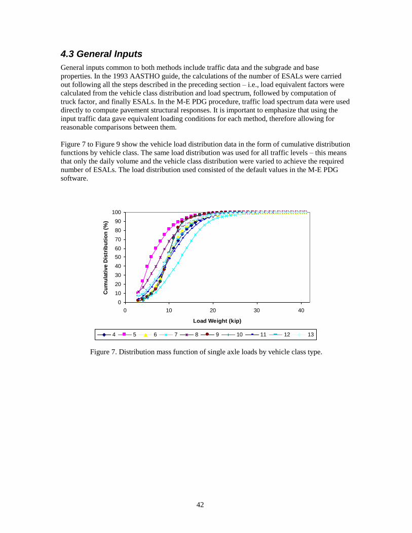
42
4.3 General Inputs
General inputs common to both methods include traffic data and the subgrade and base
properties. In the 1993 AASTHO guide, the calculations of the number of ESALs were carried
out following all the steps described in the preceding section – i.e., load equivalent factors were
calculated from the vehicle class distribution and load spectrum, followed by computation of
truck factor, and finally ESALs. In the M-E PDG procedure, traffic load spectrum data were used
directly to compute pavement structural responses. It is important to emphasize that using the
input traffic data gave equivalent loading conditions for each method, therefore allowing for
reasonable comparisons between them.
Figure 7 to Figure 9 show the vehicle load distribution data in the form of cumulative distribution
functions by vehicle class. The same load distribution was used for all traffic levels – this means
that only the daily volume and the vehicle class distribution were varied to achieve the required
number of ESALs. The load distribution used consisted of the default values in the M-E PDG
software.
0
10
20
30
40
50
60
70
80
90
100
0 10 20 30 40
Load Weight (kip)
Cu
mu
lati
ve D
istr
ibu
tio
n (
%)
4 5 6 7 8 9 10 11 12 13
Figure 7. Distribution mass function of single axle loads by vehicle class type.
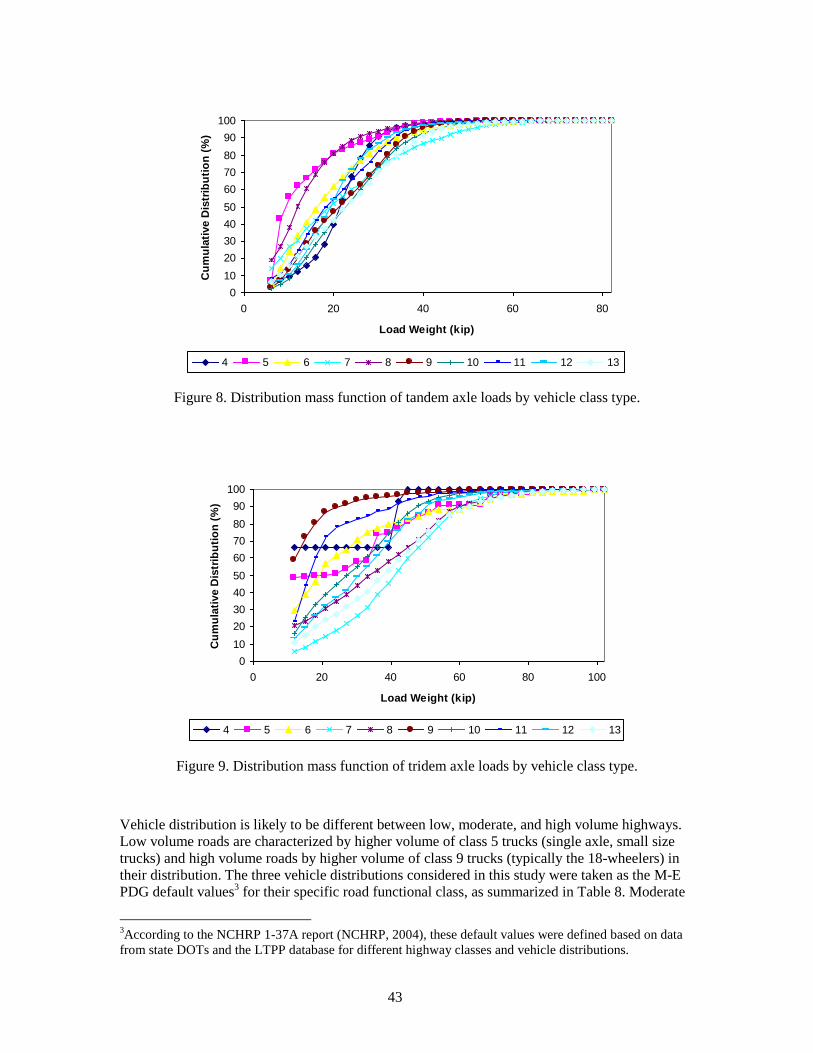
43
0
10
20
30
40
50
60
70
80
90
100
0 20 40 60 80
Load Weight (kip)
Cu
mu
lati
ve D
istr
ibu
tio
n (
%)
4 5 6 7 8 9 10 11 12 13
Figure 8. Distribution mass function of tandem axle loads by vehicle class type.
0
10
20
30
40
50
60
70
80
90
100
0 20 40 60 80 100
Load Weight (kip)
Cu
mu
lati
ve D
istr
ibu
tio
n (
%)
4 5 6 7 8 9 10 11 12 13
Figure 9. Distribution mass function of tridem axle loads by vehicle class type.
Vehicle distribution is likely to be different between low, moderate, and high volume highways.
Low volume roads are characterized by higher volume of class 5 trucks (single axle, small size
trucks) and high volume roads by higher volume of class 9 trucks (typically the 18-wheelers) in
their distribution. The three vehicle distributions considered in this study were taken as the M-E
PDG default values3 for their specific road functional class, as summarized in Table 8. Moderate
3According to the NCHRP 1-37A report (NCHRP, 2004), these default values were defined based on data
from state DOTs and the LTPP database for different highway classes and vehicle distributions.
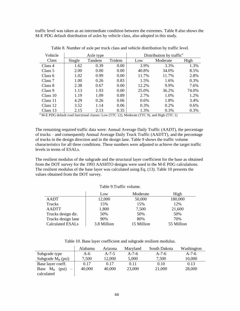
44
traffic level was taken as an intermediate condition between the extremes. Table 8 also shows the
M-E PDG default distribution of axles by vehicle class, also adopted in this study.
Table 8. Number of axle per truck class and vehicle distribution by traffic level.
Vehicle
Class
Axle type Distribution by traffica
Single Tandem Tridem Low Moderate High
Class 4 1.62 0.39 0.00 3.9% 3.3% 1.3%
Class 5 2.00 0.00 0.00 40.8% 34.0% 8.5%
Class 6 1.02 0.99 0.00 11.7% 11.7% 2.8%
Class 7 1.00 0.26 0.83 1.5% 1.6% 0.3%
Class 8 2.38 0.67 0.00 12.2% 9.9% 7.6%
Class 9 1.13 1.93 0.00 25.0% 36.2% 74.0%
Class 10 1.19 1.09 0.89 2.7% 1.0% 1.2%
Class 11 4.29 0.26 0.06 0.6% 1.8% 3.4%
Class 12 3.52 1.14 0.06 0.3% 0.2% 0.6%
Class 13 2.15 2.13 0.35 1.3% 0.3% 0.3% a M-E PDG default road functional classes: Low (TTC 12), Moderate (TTC 9), and High (TTC 1)
The remaining required traffic data were: Annual Average Daily Traffic (AADT), the percentage
of trucks – and consequently Annual Average Daily Truck Traffic (AADTT), and the percentage
of trucks in the design direction and in the design lane. Table 9 shows the traffic volume
characteristics for all three conditions. These numbers were adjusted to achieve the target traffic
levels in terms of ESALs.
The resilient modulus of the subgrade and the structural layer coefficient for the base as obtained
from the DOT survey for the 1993 AASHTO designs were used in the M-E PDG calculations.
The resilient modulus of the base layer was calculated using Eq. (13). Table 10 presents the
values obtained from the DOT survey.
Table 9.Traffic volume.
Low Moderate High
AADT 12,000 50,000 180,000
Trucks 15% 15% 12%
AADTT 1,800 7,500 21,600
Trucks design dir. 50% 50% 50%
Trucks design lane 90% 80% 70%
Calculated ESALs 3.8 Million 15 Million 55 Million
Table 10. Base layer coefficient and subgrade resilient modulus.
Alabama Arizona Maryland South Dakota Washington
Subgrade type A-6 A-7-5 A-7-6 A-7-6 A-7-6
Subgrade MR (psi) 7,500 12,000 5,000 7,500 10,000
Base layer coeff. 0.17 0.17 0.11 0.10 0.13
Base MR (psi) –
calculated
40,000 40,000 23,000 21,000 28,000
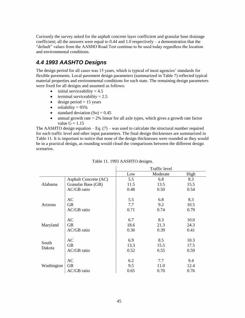
45
Curiously the survey asked for the asphalt concrete layer coefficient and granular base drainage
coefficient; all the answers were equal to 0.44 and 1.0 respectively – a demonstration that the
―default‖ values from the AASHO Road Test continue to be used today regardless the location
and environmental conditions.
4.4 1993 AASHTO Designs
The design period for all cases was 15 years, which is typical of most agencies’ standards for
flexible pavements. Local pavement design parameters (summarized in Table 7) reflected typical
material properties and environmental conditions for each state. The remaining design parameters
were fixed for all designs and assumed as follows:
initial serviceability = 4.5
terminal serviceability = 2.5
design period = 15 years
reliability = 95%
standard deviation (So) = 0.45
annual growth rate = 2% linear for all axle types, which gives a growth rate factor
value G = 1.15
The AASHTO design equation – Eq. (7) – was used to calculate the structural number required
for each traffic level and other input parameters. The final design thicknesses are summarized in
Table 11. It is important to notice that none of the design thicknesses were rounded as they would
be in a practical design, as rounding would cloud the comparisons between the different design
scenarios.
Table 11. 1993 AASHTO designs.
Traffic level
Low Moderate High
Alabama
Asphalt Concrete (AC) 5.5 6.8 8.3
Granular Base (GB) 11.5 13.5 15.5
AC/GB ratio 0.48 0.50 0.54
Arizona
AC 5.5 6.8 8.3
GB 7.7 9.2 10.5
AC/GB ratio 0.71 0.74 0.79
Maryland
AC 6.7 8.3 10.0
GB 18.6 21.3 24.3
AC/GB ratio 0.36 0.39 0.41
South
Dakota
AC 6.9 8.5 10.3
GB 13.3 15.5 17.5
AC/GB ratio 0.52 0.55 0.59
Washington
AC 6.2 7.7 9.4
GB 9.5 11.0 12.4
AC/GB ratio 0.65 0.70 0.76
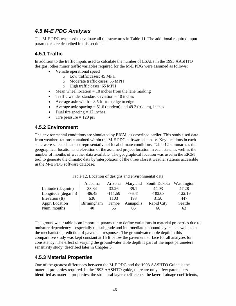
46
4.5 M-E PDG Analysis
The M-E PDG was used to evaluate all the structures in Table 11. The additional required input
parameters are described in this section.
4.5.1 Traffic
In addition to the traffic inputs used to calculate the number of ESALs in the 1993 AASHTO
designs, other minor traffic variables required for the M-E PDG were assumed as follows:
Vehicle operational speed
o Low traffic cases: 45 MPH
o Moderate traffic cases: 55 MPH
o High traffic cases: 65 MPH
Mean wheel location = 18 inches from the lane marking
Traffic wander standard deviation = 10 inches
Average axle width = 8.5 ft from edge to edge
Average axle spacing = 51.6 (tandem) and 49.2 (tridem), inches
Dual tire spacing = 12 inches
Tire pressure = 120 psi
4.5.2 Environment
The environmental conditions are simulated by EICM, as described earlier. This study used data
from weather stations contained within the M-E PDG software database. Key locations in each
state were selected as most representative of local climate conditions. Table 12 summarizes the
geographical location and elevation of the assumed project location in each state, as well as the
number of months of weather data available. The geographical location was used in the EICM
tool to generate the climatic data by interpolation of the three closest weather stations accessible
in the M-E PDG software database.
Table 12. Location of designs and environmental data.
Alabama Arizona Maryland South Dakota Washington
Latitude (deg.min) 33.34 33.26 39.1 44.03 47.28
Longitude (deg.min) -86.45 -111.59 -76.41 -103.03 -122.19
Elevation (ft) 636 1103 193 3150 447
Appr. Location Birmingham Tempe Annapolis Rapid City Seattle
Num. months 40 66 66 66 63
The groundwater table is an important parameter to define variations in material properties due to
moisture dependency – especially the subgrade and intermediate unbound layers – as well as in
the mechanistic prediction of pavement responses. The groundwater table depth in this
comparative study was kept constant at 15 ft below the pavement surface for all analyses for
consistency. The effect of varying the groundwater table depth is part of the input parameters
sensitivity study, described later in Chapter 5.
4.5.3 Material Properties
One of the greatest differences between the M-E PDG and the 1993 AASHTO Guide is the
material properties required. In the 1993 AASHTO guide, there are only a few parameters
identified as material properties: the structural layer coefficients, the layer drainage coefficients,

47
and the subgrade resilient modulus. These parameters are not enough to describe complex
material behavior such as stress-dependent stiffness of unbound materials and time- and
temperature-dependent response of asphalt mixtures.
The M-E PDG requires engineering properties of layer materials for a mechanistic analysis of
pavement responses (either using elastic theory or the finite element method). In the case of
flexible pavements, these properties are (1) dynamic modulus for asphalt mixtures, and (2)
resilient modulus for unbound materials. These properties are also environment-dependent, and
seasonal variations in temperature and moisture affect their values. The EICM predicts variations
of temperature and moisture throughout the seasons and within the pavement structure that are
used to adjust the material property for that particular environmental condition.
As mentioned before, the hierarchical input approach provides three input levels depending on the
quality of the data. For example, level 1 for asphalt concrete is based on laboratory-measured
dynamic modulus while levels 2 and 3 rely on predicted dynamic modulus based on binder
properties, mixture gradation, and volumetric properties. Level 3 material property inputs were
used in this study. These are judged to be most consistent with the quality of material inputs used
in the 1993 AASHTO procedure. It also represents the expected input level to be used by most
agencies at the beginning of the M-E PDG implementation.
A set of typical material properties was selected for the asphalt concrete and granular base. The
same asphalt concrete volumetrics and gradation were used with all cases, with the exception of
binder type. The LTPPBIND® software (LTPPBIND
®, version 2.1, 1999) was used to determine
the optimal binder grade at each geographical location and traffic volume. For each state, the
typical subgrade soil type was provided by the agencies as part of the survey, along with the
resilient modulus.
The M-E PDG requires the subgrade resilient modulus at optimum moisture and density.
Alabama and Maryland’s DOT indicated in the survey that they do not seasonally adjust subgrade
resilient modulus. Arizona and South Dakota did not provide this information, and Washington
uses the effective or seasonally adjusted resilient modulus for subgrade materials. All values used
in this study were taken as at optimum moisture and density because they were within expected
ranges typical of their soil type found in the literature as well as in the M-E PDG software. The
material properties used for the M-E PDG analyses in this study are summarized in Table 13
through Table 18.
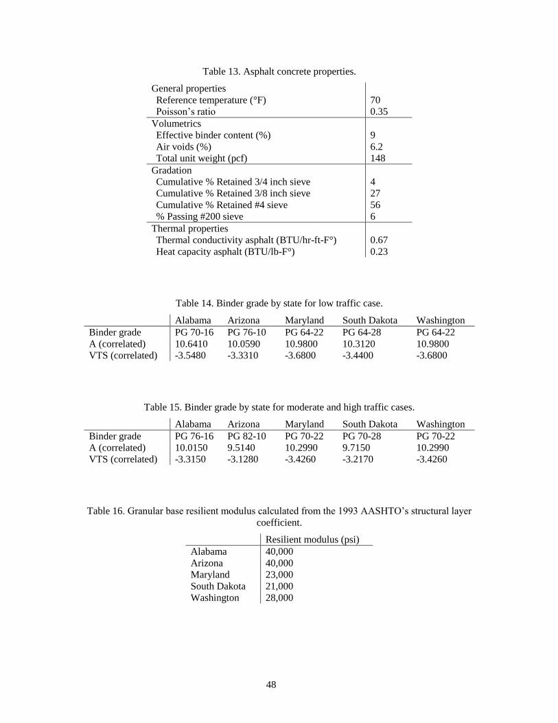
48
Table 13. Asphalt concrete properties.
General properties
Reference temperature (°F) 70
Poisson’s ratio 0.35
Volumetrics
Effective binder content (%) 9
Air voids (%) 6.2
Total unit weight (pcf) 148
Gradation
Cumulative % Retained 3/4 inch sieve 4
Cumulative % Retained 3/8 inch sieve 27
Cumulative % Retained #4 sieve 56
% Passing #200 sieve 6
Thermal properties
Thermal conductivity asphalt (BTU/hr-ft-F°) 0.67
Heat capacity asphalt (BTU/lb-F°) 0.23
Table 14. Binder grade by state for low traffic case.
Alabama Arizona Maryland South Dakota Washington
Binder grade PG 70-16 PG 76-10 PG 64-22 PG 64-28 PG 64-22
A (correlated) 10.6410 10.0590 10.9800 10.3120 10.9800
VTS (correlated) -3.5480 -3.3310 -3.6800 -3.4400 -3.6800
Table 15. Binder grade by state for moderate and high traffic cases.
Alabama Arizona Maryland South Dakota Washington
Binder grade PG 76-16 PG 82-10 PG 70-22 PG 70-28 PG 70-22
A (correlated) 10.0150 9.5140 10.2990 9.7150 10.2990
VTS (correlated) -3.3150 -3.1280 -3.4260 -3.2170 -3.4260
Table 16. Granular base resilient modulus calculated from the 1993 AASHTO’s structural layer
coefficient.
Resilient modulus (psi)
Alabama 40,000
Arizona 40,000
Maryland 23,000
South Dakota 21,000
Washington 28,000
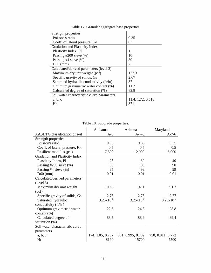
49
Table 17. Granular aggregate base properties.
Strength properties
Poisson's ratio 0.35
Coeff. of lateral pressure, Ko 0.5
Gradation and Plasticity Index
Plasticity Index, PI 1
Passing #200 sieve (%) 10
Passing #4 sieve (%) 80
D60 (mm) 2
Calculated/derived parameters (level 3)
Maximum dry unit weight (pcf) 122.3
Specific gravity of solids, Gs 2.67
Saturated hydraulic conductivity (ft/hr) 37
Optimum gravimetric water content (%) 11.2
Calculated degree of saturation (%) 82.8
Soil water characteristic curve parameters
a, b, c 11.4; 1.72; 0.518
Hr 371
Table 18. Subgrade properties.
Alabama Arizona Maryland
AASHTO classification of soil A-6 A-7-5 A-7-6
Strength properties
Poisson's ratio 0.35 0.35 0.35
Coeff. of lateral pressure, KO 0.5 0.5 0.5
Resilient modulus (psi) 7,500 12,000 5,000
Gradation and Plasticity Index
Plasticity Index, PI 25 30 40
Passing #200 sieve (%) 80 85 90
Passing #4 sieve (%) 95 99 99
D60 (mm) 0.01 0.01 0.01
Calculated/derived parameters
(level 3)
Maximum dry unit weight
(pcf)
100.8 97.1 91.3
Specific gravity of solids, Gs 2.75 2.75 2.77
Saturated hydraulic
conductivity (ft/hr)
3.25x10⁻⁵
3.25x10⁻⁵
3.25x10⁻⁵
Optimum gravimetric water
content (%)
22.6 24.8 28.8
Calculated degree of
saturation (%)
88.5 88.9 89.4
Soil water characteristic curve
parameters
a, b, c 174; 1.05; 0.707 301; 0.995; 0.732 750; 0.911; 0.772
Hr 8190 15700 47500
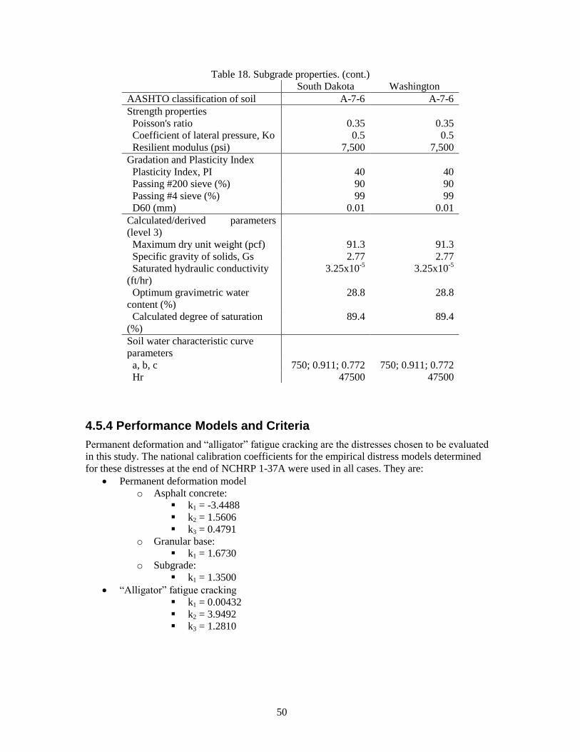
50
Table 18. Subgrade properties. (cont.)
South Dakota Washington
AASHTO classification of soil A-7-6 A-7-6
Strength properties
Poisson's ratio 0.35 0.35
Coefficient of lateral pressure, Ko 0.5 0.5
Resilient modulus (psi) 7,500 7,500
Gradation and Plasticity Index
Plasticity Index, PI 40 40
Passing #200 sieve (%) 90 90
Passing #4 sieve (%) 99 99
D60 (mm) 0.01 0.01
Calculated/derived parameters
(level 3)
Maximum dry unit weight (pcf) 91.3 91.3
Specific gravity of solids, Gs 2.77 2.77
Saturated hydraulic conductivity
(ft/hr)
3.25x10⁻⁵
3.25x10⁻⁵
Optimum gravimetric water
content (%)
28.8 28.8
Calculated degree of saturation
(%)
89.4 89.4
Soil water characteristic curve
parameters
a, b, c 750; 0.911; 0.772 750; 0.911; 0.772
Hr 47500 47500
4.5.4 Performance Models and Criteria
Permanent deformation and ―alligator‖ fatigue cracking are the distresses chosen to be evaluated
in this study. The national calibration coefficients for the empirical distress models determined
for these distresses at the end of NCHRP 1-37A were used in all cases. They are:
Permanent deformation model
o Asphalt concrete:
k1 = -3.4488
k2 = 1.5606
k3 = 0.4791
o Granular base:
k1 = 1.6730
o Subgrade:
k1 = 1.3500
―Alligator‖ fatigue cracking
k1 = 0.00432
k2 = 3.9492
k3 = 1.2810
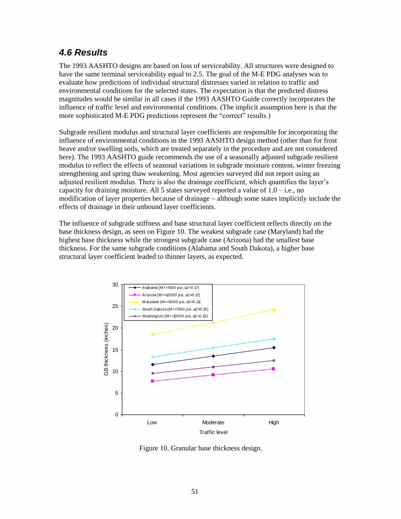
51
4.6 Results
The 1993 AASHTO designs are based on loss of serviceability. All structures were designed to
have the same terminal serviceability equal to 2.5. The goal of the M-E PDG analyses was to
evaluate how predictions of individual structural distresses varied in relation to traffic and
environmental conditions for the selected states. The expectation is that the predicted distress
magnitudes would be similar in all cases if the 1993 AASHTO Guide correctly incorporates the
influence of traffic level and environmental conditions. (The implicit assumption here is that the
more sophisticated M-E PDG predictions represent the ―correct‖ results.)
Subgrade resilient modulus and structural layer coefficients are responsible for incorporating the
influence of environmental conditions in the 1993 AASHTO design method (other than for frost
heave and/or swelling soils, which are treated separately in the procedure and are not considered
here). The 1993 AASHTO guide recommends the use of a seasonally adjusted subgrade resilient
modulus to reflect the effects of seasonal variations in subgrade moisture content, winter freezing
strengthening and spring thaw weakening. Most agencies surveyed did not report using an
adjusted resilient modulus. There is also the drainage coefficient, which quantifies the layer’s
capacity for draining moisture. All 5 states surveyed reported a value of 1.0 – i.e., no
modification of layer properties because of drainage – although some states implicitly include the
effects of drainage in their unbound layer coefficients.
The influence of subgrade stiffness and base structural layer coefficient reflects directly on the
base thickness design, as seen on Figure 10. The weakest subgrade case (Maryland) had the
highest base thickness while the strongest subgrade case (Arizona) had the smallest base
thickness. For the same subgrade conditions (Alabama and South Dakota), a higher base
structural layer coefficient leaded to thinner layers, as expected.
0
5
10
15
20
25
30
Low Moderate High
Traff ic level
GB
thic
kness (
inches)
Alabama (M r=7500 psi, a2=0.17)
Arizona (M r=12000 psi, a2=0.17)
M aryland (M r=5000 psi, a2=0.11)
South Dakota (M r=7500 psi, a2=0.10)
Washington (M r=10000 psi, a2=0.13)
Figure 10. Granular base thickness design.
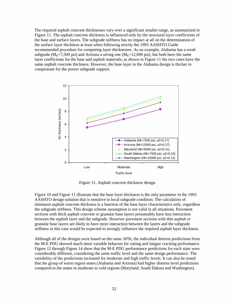
52
The required asphalt concrete thicknesses vary over a significant smaller range, as summarized in
Figure 11. The asphalt concrete thickness is influenced only by the structural layer coefficients of
the base and surface layers. The subgrade stiffness has no impact at all on the determination of
the surface layer thickness at least when following strictly the 1993 AASHTO Guide
recommended procedure for computing layer thicknesses. As an example, Alabama has a weak
subgrade (MR=7,500 psi) and Arizona a strong one (MR=12,000 psi), but both have the same
layer coefficients for the base and asphalt materials; as shown in Figure 11 the two cases have the
same asphalt concrete thickness. However, the base layer in the Alabama design is thicker to
compensate for the poorer subgrade support.
0
2
4
6
8
10
12
Low Moderate High
Traff ic level
AC
thic
kness (
inches)
Alabama (Mr=7500 psi, a2=0.17)
Arizona (Mr=12000 psi, a2=0.17)
Maryland (Mr=5000 psi, a2=0.11)
South Dakota (Mr=7500 psi, a2=0.10)
Washington (Mr=10000 psi, a2=0.13)
Figure 11. Asphalt concrete thickness design.
Figure 10 and Figure 11 illustrate that the base layer thickness is the only parameter in the 1993
AASHTO design solution that is sensitive to local subgrade condition. The calculation of
minimum asphalt concrete thickness is a function of the base layer characteristics only, regardless
the subgrade stiffness. This design scheme assumption is not valid in all situations. Pavement
sections with thick asphalt concrete or granular base layers presumably have less interaction
between the asphalt layer and the subgrade. However pavement sections with thin asphalt or
granular base layers are likely to have more interaction between the layers and the subgrade
stiffness in this case would be expected to strongly influence the required asphalt layer thickness.
Although all of the designs were based on the same PSI, the individual distress predictions from
the M-E PDG showed much more variable behavior for rutting and fatigue cracking performance.
Figure 12 through Figure 14 show that the M-E PDG performance predictions for each state were
considerably different, considering the same traffic level and the same design performance. The
variability of the predictions increased for moderate and high traffic levels. It can also be noted
that the group of warm region states (Alabama and Arizona) had higher distress level predictions
compared to the states in moderate to cold regions (Maryland, South Dakota and Washington).
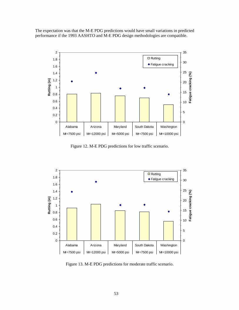
53
The expectation was that the M-E PDG predictions would have small variations in predicted
performance if the 1993 AASHTO and M-E PDG design methodologies are compatible.
0
0.2
0.4
0.6
0.8
1
1.2
1.4
1.6
1.8
2
Alabama Arizona Maryland South Dakota Washington
Mr=7500 psi Mr=12000 psi Mr=5000 psi Mr=7500 psi Mr=10000 psi
Ru
ttin
g (
in)
0
5
10
15
20
25
30
35
Fati
gu
e c
rackin
g (
%)
Rutting
Fatigue cracking
Figure 12. M-E PDG predictions for low traffic scenario.
0
0.2
0.4
0.6
0.8
1
1.2
1.4
1.6
1.8
2
Alabama Arizona Maryland South Dakota Washington
Mr=7500 psi Mr=12000 psi Mr=5000 psi Mr=7500 psi Mr=10000 psi
Ru
ttin
g (
in)
0
5
10
15
20
25
30
35
Fati
gu
e c
rackin
g (
%)
Rutting
Fatigue cracking
Figure 13. M-E PDG predictions for moderate traffic scenario.

54
0
0.2
0.4
0.6
0.8
1
1.2
1.4
1.6
1.8
2
Alabama Arizona Maryland South Dakota Washington
Mr=7500 psi Mr=12000 psi Mr=5000 psi Mr=7500 psi Mr=10000 psi
Ru
ttin
g (
in)
0
5
10
15
20
25
30
35
Fati
gu
e c
rackin
g (
%)
Rutting
Fatigue cracking
Figure 14. M-E PDG predictions for high traffic scenario.
The performance predictions for moderate and high traffic scenarios exceeded acceptable limits.
In the case of rutting, for example, a survey conducted by Witczak among pavement engineers in
several state agencies suggests an acceptable total rutting limit of 0.5 inches on average, before
adjustment for reliability (Witczak, 2004). The M-E PDG procedure recommends an acceptable
total rutting limit of 0.75 inches after adjustment for reliability.
States located in the warmest zone (Alabama and Arizona) consistently had poorer performance
than the other states located in mild to low temperature areas. The AASHO Road Test site, the
data source for developing the 1993 AASHTO Guide, was located in Ottawa, IL, a low
temperature region. The results here suggest that, at least according to the M-E PDG, the 1993
AASHTO Guide overestimates the performance (or underestimates the required thickness) of
pavement sections at locations having warmer temperatures than the original AASHO Road Test
site.
It can also be noted from Figure 12 through Figure 14 that the performance consistently
deteriorated as traffic increased in all five states. Figure 15 summarizes the M-E PDG predictions
for the three traffic levels of all states in which it can be seen that performance consistently
deteriorated for both rutting and fatigue cracking as traffic increased in all five states. These
results suggest that the 1993 AASHTO guide overestimates pavement performance for traffic
levels well beyond those experienced in the AASHO Road Test (under 2 Million ESALs).
The alternate interpretation is that the M-E PDG may be overestimating rutting and fatigue
cracking, but this seems less likely given the larger set of field pavement sections incorporated in
its calibration and the consistency within the predictions for the low traffic scenario at locations
having moderate to low temperatures—i.e., for conditions similar to those in the original AASHO
Road Test results underlying the 1993 AASHTO guide.
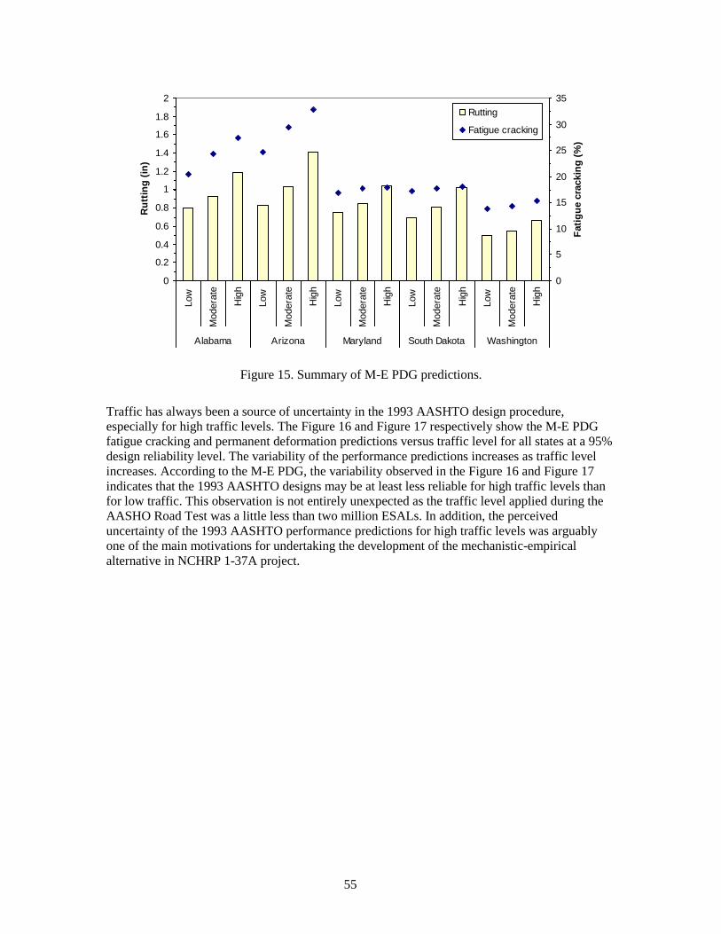
55
0
0.2
0.4
0.6
0.8
1
1.2
1.4
1.6
1.8
2
Low
Modera
te
Hig
h
Low
Modera
te
Hig
h
Low
Modera
te
Hig
h
Low
Modera
te
Hig
h
Low
Modera
te
Hig
h
Alabama Arizona Maryland South Dakota Washington
Ru
ttin
g (
in)
0
5
10
15
20
25
30
35
Fati
gu
e c
rackin
g (
%)
Rutting
Fatigue cracking
Figure 15. Summary of M-E PDG predictions.
Traffic has always been a source of uncertainty in the 1993 AASHTO design procedure,
especially for high traffic levels. The Figure 16 and Figure 17 respectively show the M-E PDG
fatigue cracking and permanent deformation predictions versus traffic level for all states at a 95%
design reliability level. The variability of the performance predictions increases as traffic level
increases. According to the M-E PDG, the variability observed in the Figure 16 and Figure 17
indicates that the 1993 AASHTO designs may be at least less reliable for high traffic levels than
for low traffic. This observation is not entirely unexpected as the traffic level applied during the
AASHO Road Test was a little less than two million ESALs. In addition, the perceived
uncertainty of the 1993 AASHTO performance predictions for high traffic levels was arguably
one of the main motivations for undertaking the development of the mechanistic-empirical
alternative in NCHRP 1-37A project.
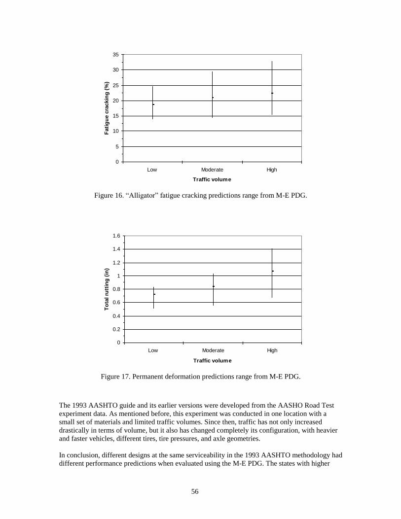
56
0
5
10
15
20
25
30
35
Low Moderate High
Traffic volume
Fati
gu
e c
rackin
g (
%)
Figure 16. ―Alligator‖ fatigue cracking predictions range from M-E PDG.
0
0.2
0.4
0.6
0.8
1
1.2
1.4
1.6
Low Moderate High
Traffic volume
To
tal ru
ttin
g (
in)
Figure 17. Permanent deformation predictions range from M-E PDG.
The 1993 AASHTO guide and its earlier versions were developed from the AASHO Road Test
experiment data. As mentioned before, this experiment was conducted in one location with a
small set of materials and limited traffic volumes. Since then, traffic has not only increased
drastically in terms of volume, but it also has changed completely its configuration, with heavier
and faster vehicles, different tires, tire pressures, and axle geometries.
In conclusion, different designs at the same serviceability in the 1993 AASHTO methodology had
different performance predictions when evaluated using the M-E PDG. The states with higher

57
average temperatures had worse performance than those with mild to low average temperatures,
indicating that the 1993 AASHTO Guide possibly overestimates the performance (or
underestimates the required pavement thickness) for the warm locations.
When comparisons with traffic levels were made it was found that the performance predicted by
the M-E PDG deteriorated as traffic level increased. The results also showed that performance
prediction variability increased with increasing traffic level. The traffic analysis indicates that the
1993 AASHTO Guide may overestimate performance (or underestimate required pavement
thickness) when traffic levels are well beyond those in the AASHO Road Test.
The following chapter will concentrate on evaluating the M-E PDG and the sensitivity of
pavement performance to input parameters. The results are compared with field expectations for
reasonableness.

58
5. M-E PDG Sensitivity to Inputs
Parametric studies are an important step in any implementation of the M-E PDG as a new
pavement design standard in highway agencies. The results and conclusions are useful for
developing knowledge about the procedure, finding weaknesses and problems within the local
agencies’ practice that need to be addressed, and defining priorities for the implementation and
calibration tasks.
The objective of the parametric study in this Chapter is to provide useful and relevant data
analyses of performance prediction sensitivity to input parameters and to evaluate the results
against engineering expectations of real field performance.
The pavement structure designed with the 1993 AASHTO guide for low traffic Maryland
conditions (see Table 11) was the reference case for this parametric study. The variables selected
for study were: asphalt and base layer thickness, traffic, environment, material properties,
performance model parameters, and design criteria. Only level 3 inputs were used in this
parametric study.
Parameters were varied by a percentage of their reference design values. When percentage
variation was not possible, distinct cases were selected for comparison purpose (i.e., mixture type,
vehicle class distribution, climate conditions, etc.).
5.1 Thickness
The thickness parametric study considered asphalt and base layers, with variations of 20% above
and below the reference design – 6.7 inches and 18.6 inches respectively. The results in Figure 18
indicate that base layer thickness has little influence on performance in the M-E PDG
methodology. Alligator fatigue cracking slightly decreases with increased base thickness, while
the permanent deformation variation was negligible. This result is significantly different from
trends in the 1993 AASHTO guide, in which the base layer thickness has considerable influence
on the structural number (SN) and consequently on PSI prediction.
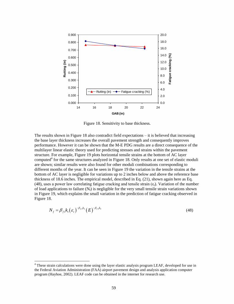
59
0.000
0.100
0.200
0.300
0.400
0.500
0.600
0.700
0.800
0.900
14 16 18 20 22 24
GAB (in)
Ru
ttin
g (
in)
0.0
2.0
4.0
6.0
8.0
10.0
12.0
14.0
16.0
18.0
20.0
Fati
gu
e c
rackin
g (
%)
Rutting (in) Fatigue cracking (%)
Figure 18. Sensitivity to base thickness.
The results shown in Figure 18 also contradict field expectations – it is believed that increasing
the base layer thickness increases the overall pavement strength and consequently improves
performance. However it can be shown that the M-E PDG results are a direct consequence of the
multilayer linear elastic theory used for predicting stresses and strains within the pavement
structure. For example, Figure 19 plots horizontal tensile strains at the bottom of AC layer
computed4 for the same structures analyzed in Figure 18. Only results at one set of elastic moduli
are shown; similar results were also found for other moduli combinations corresponding to
different months of the year. It can be seen in Figure 19 the variation in the tensile strains at the
bottom of AC layer is negligible for variations up to 2 inches below and above the reference base
thickness of 18.6 inches. The empirical model, described in Eq. (21), shown again here as Eq.
(48), uses a power law correlating fatigue cracking and tensile strain (εt). Variation of the number
of load applications to failure (Nf) is negligible for the very small tensile strain variations shown
in Figure 19, which explains the small variation in the prediction of fatigue cracking observed in
Figure 18.
2 2 3 3
1 1
f fk k
f f tN k E
(48)
4 These strain calculations were done using the layer elastic analysis program LEAF, developed for use in
the Federal Aviation Administration (FAA) airport pavement design and analysis application computer
program (Hayhoe, 2002). LEAF code can be obtained in the internet for research use.
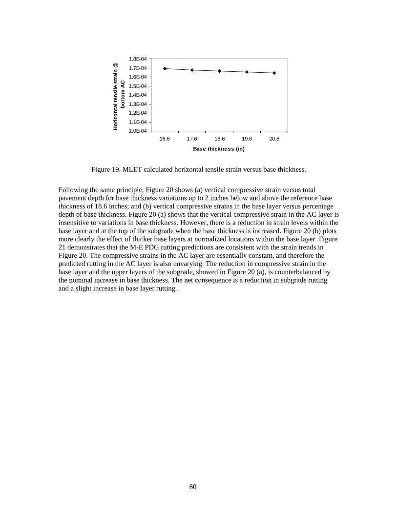
60
1.0E-04
1.1E-04
1.2E-04
1.3E-04
1.4E-04
1.5E-04
1.6E-04
1.7E-04
1.8E-04
16.6 17.6 18.6 19.6 20.6
Base thickness (in)
Ho
rizo
nta
l te
nsile s
train
@
bo
tto
m A
C
Figure 19. MLET calculated horizontal tensile strain versus base thickness.
Following the same principle, Figure 20 shows (a) vertical compressive strain versus total
pavement depth for base thickness variations up to 2 inches below and above the reference base
thickness of 18.6 inches; and (b) vertical compressive strains in the base layer versus percentage
depth of base thickness. Figure 20 (a) shows that the vertical compressive strain in the AC layer is
insensitive to variations in base thickness. However, there is a reduction in strain levels within the
base layer and at the top of the subgrade when the base thickness is increased. Figure 20 (b) plots
more clearly the effect of thicker base layers at normalized locations within the base layer. Figure
21 demonstrates that the M-E PDG rutting predictions are consistent with the strain trends in
Figure 20. The compressive strains in the AC layer are essentially constant, and therefore the
predicted rutting in the AC layer is also unvarying. The reduction in compressive strain in the
base layer and the upper layers of the subgrade, showed in Figure 20 (a), is counterbalanced by
the nominal increase in base thickness. The net consequence is a reduction in subgrade rutting
and a slight increase in base layer rutting.
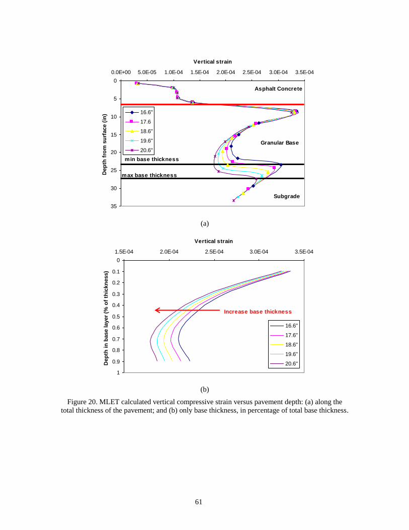
61
0
5
10
15
20
25
30
35
0.0E+00 5.0E-05 1.0E-04 1.5E-04 2.0E-04 2.5E-04 3.0E-04 3.5E-04
Vertical strain
Dep
th f
rom
su
rface (
in) 16.6''
17.6
18.6''
19.6''
20.6''
Asphalt Concrete
Granular Base
Subgrade
min base thickness
max base thickness
(a)
0
0.1
0.2
0.3
0.4
0.5
0.6
0.7
0.8
0.9
1
1.5E-04 2.0E-04 2.5E-04 3.0E-04 3.5E-04
Vertical strain
Dep
th in
base layer
(% o
f th
ickn
ess)
16.6''
17.6''
18.6''
19.6''
20.6''
Increase base thickness
(b)
Figure 20. MLET calculated vertical compressive strain versus pavement depth: (a) along the
total thickness of the pavement; and (b) only base thickness, in percentage of total base thickness.
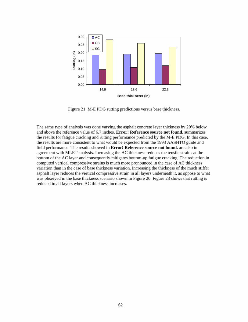
62
0.00
0.05
0.10
0.15
0.20
0.25
0.30
14.9 18.6 22.3
Base thickness (in)
Ru
ttin
g (
in)
AC
GB
SG
Figure 21. M-E PDG rutting predictions versus base thickness.
The same type of analysis was done varying the asphalt concrete layer thickness by 20% below
and above the reference value of 6.7 inches. Error! Reference source not found. summarizes
the results for fatigue cracking and rutting performance predicted by the M-E PDG. In this case,
the results are more consistent to what would be expected from the 1993 AASHTO guide and
field performance. The results showed in Error! Reference source not found. are also in
agreement with MLET analysis. Increasing the AC thickness reduces the tensile strains at the
bottom of the AC layer and consequently mitigates bottom-up fatigue cracking. The reduction in
computed vertical compressive strains is much more pronounced in the case of AC thickness
variation than in the case of base thickness variation. Increasing the thickness of the much stiffer
asphalt layer reduces the vertical compressive strain in all layers underneath it, as oppose to what
was observed in the base thickness scenario shown in Figure 20. Figure 23 shows that rutting is
reduced in all layers when AC thickness increases.
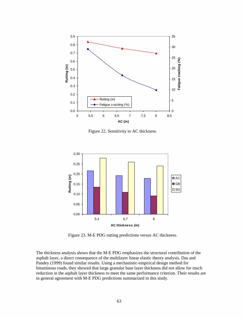
63
0.0
0.1
0.2
0.3
0.4
0.5
0.6
0.7
0.8
0.9
5 5.5 6 6.5 7 7.5 8 8.5
AC (in)
Ru
ttin
g (
in)
0
5
10
15
20
25
30
35
Fati
gu
e c
rackin
g (
%)
Rutting (in)
Fatigue cracking (%)
Figure 22. Sensitivity to AC thickness.
0.00
0.05
0.10
0.15
0.20
0.25
0.30
5.4 6.7 8
AC thickness (in)
Ru
ttin
g (
in)
AC
GB
SG
Figure 23. M-E PDG rutting predictions versus AC thickness.
The thickness analysis shows that the M-E PDG emphasizes the structural contribution of the
asphalt layer, a direct consequence of the multilayer linear elastic theory analysis. Das and
Pandey (1999) found similar results. Using a mechanistic-empirical design method for
bituminous roads, they showed that large granular base layer thickness did not allow for much
reduction in the asphalt layer thickness to meet the same performance criterion. Their results are
in general agreement with M-E PDG predictions summarized in this study.
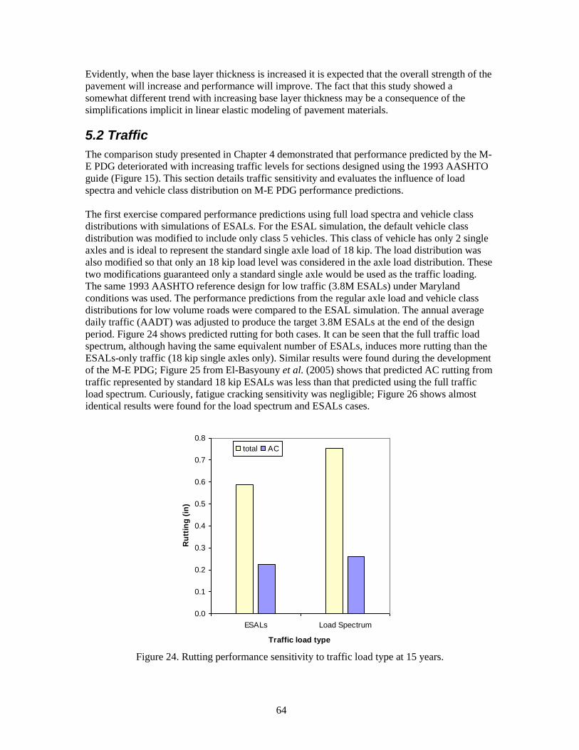
64
Evidently, when the base layer thickness is increased it is expected that the overall strength of the
pavement will increase and performance will improve. The fact that this study showed a
somewhat different trend with increasing base layer thickness may be a consequence of the
simplifications implicit in linear elastic modeling of pavement materials.
5.2 Traffic
The comparison study presented in Chapter 4 demonstrated that performance predicted by the M-
E PDG deteriorated with increasing traffic levels for sections designed using the 1993 AASHTO
guide (Figure 15). This section details traffic sensitivity and evaluates the influence of load
spectra and vehicle class distribution on M-E PDG performance predictions.
The first exercise compared performance predictions using full load spectra and vehicle class
distributions with simulations of ESALs. For the ESAL simulation, the default vehicle class
distribution was modified to include only class 5 vehicles. This class of vehicle has only 2 single
axles and is ideal to represent the standard single axle load of 18 kip. The load distribution was
also modified so that only an 18 kip load level was considered in the axle load distribution. These
two modifications guaranteed only a standard single axle would be used as the traffic loading.
The same 1993 AASHTO reference design for low traffic (3.8M ESALs) under Maryland
conditions was used. The performance predictions from the regular axle load and vehicle class
distributions for low volume roads were compared to the ESAL simulation. The annual average
daily traffic (AADT) was adjusted to produce the target 3.8M ESALs at the end of the design
period. Figure 24 shows predicted rutting for both cases. It can be seen that the full traffic load
spectrum, although having the same equivalent number of ESALs, induces more rutting than the
ESALs-only traffic (18 kip single axles only). Similar results were found during the development
of the M-E PDG; Figure 25 from El-Basyouny et al. (2005) shows that predicted AC rutting from
traffic represented by standard 18 kip ESALs was less than that predicted using the full traffic
load spectrum. Curiously, fatigue cracking sensitivity was negligible; Figure 26 shows almost
identical results were found for the load spectrum and ESALs cases.
0.0
0.1
0.2
0.3
0.4
0.5
0.6
0.7
0.8
ESALs Load Spectrum
Traffic load type
Ru
ttin
g (
in)
total AC
Figure 24. Rutting performance sensitivity to traffic load type at 15 years.
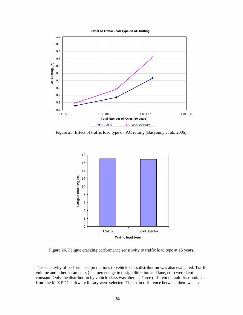
65
Figure 25. Effect of traffic load type on AC rutting (Basyouny et al., 2005).
0
2
4
6
8
10
12
14
16
18
ESALs Load Spectra
Traffic load type
Fati
gu
e c
rackin
g (
%)
Figure 26. Fatigue cracking performance sensitivity to traffic load type at 15 years.
The sensitivity of performance predictions to vehicle class distribution was also evaluated. Traffic
volume and other parameters (i.e., percentage in design direction and lane, etc.) were kept
constant. Only the distribution by vehicle class was altered. Three different default distributions
from the M-E PDG software library were selected. The main difference between them was in
Effect of Traffic Load Type on AC Rutting
0.0
0.1
0.2
0.3
0.4
0.5
0.6
0.7
0.8
0.9
1.0
1.0E+05 1.0E+06 1.0E+07 1.0E+08
Total Number of Axles (10 years)
AC
Ru
ttin
g (
in)
ESALS Load Spectrum
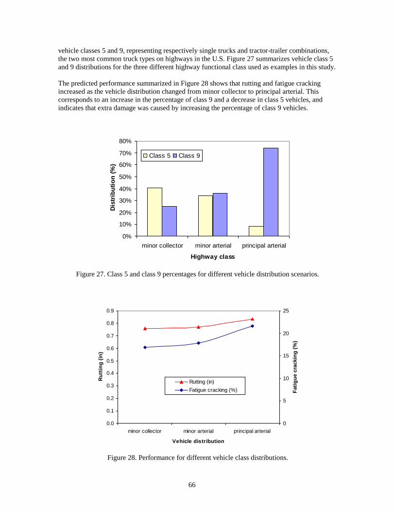
66
vehicle classes 5 and 9, representing respectively single trucks and tractor-trailer combinations,
the two most common truck types on highways in the U.S. Figure 27 summarizes vehicle class 5
and 9 distributions for the three different highway functional class used as examples in this study.
The predicted performance summarized in Figure 28 shows that rutting and fatigue cracking
increased as the vehicle distribution changed from minor collector to principal arterial. This
corresponds to an increase in the percentage of class 9 and a decrease in class 5 vehicles, and
indicates that extra damage was caused by increasing the percentage of class 9 vehicles.
0%
10%
20%
30%
40%
50%
60%
70%
80%
minor collector minor arterial principal arterial
Highway class
Dis
trib
uti
on
(%
)
Class 5 Class 9
Figure 27. Class 5 and class 9 percentages for different vehicle distribution scenarios.
0.0
0.1
0.2
0.3
0.4
0.5
0.6
0.7
0.8
0.9
minor collector minor arterial principal arterial
Vehicle distribution
Ru
ttin
g (
in)
0
5
10
15
20
25
Fati
gu
e c
rackin
g (
%)
Rutting (in)
Fatigue cracking (%)
Figure 28. Performance for different vehicle class distributions.

67
Traffic data is a fundamental parameter for pavement design. Results shown earlier in Chapter 4
indicated that performance is very sensitive to traffic volume, as expected. In addition, the results
from the present parametric study show the impacts that vehicle class and load distributions have
on performance. The concept of equivalent traffic is not adequate for representing traffic loading
in M-E designs for permanent deformation predictions. On the other hand, results for fatigue
cracking predictions were very similar, which indicate that, for low traffic scenario and this
environmental condition, equivalent traffic is suitable for this type of distress.
5.3 Environment
The climate effects were analyzed by simulating three different locations within the state of
Maryland. These locations were chosen to represent the most significant local environmental
variations. Although these locations are relatively close to one another, their climate
characteristics are sufficiently different to illustrate the effects of the Enhanced Integrated
Climate Model (EICM) on a small region.
The climate condition on Maryland Eastern Shore is dominated by the Chesapeake Bay, its
surrounding estuaries, and costal plains. This region has on average warmer temperatures and
more precipitation than the rest of the state – the annual average temperature is 56 °F and
precipitation is on the order of 43 inches. As mentioned before in earlier chapters, temperature
affects directly the stiffness of asphalt concrete mixtures, while moisture has impact on unbound
material resilient modulus. These two effects combined affect the pavement performance.
The central region is characterized by the Piedmont Plateau; it is the intermediate climate
condition, with annual average temperature in the order of 53 °F and precipitation around 40
inches. All Maryland designs in this parametric study were done for the central region location,
unless otherwise stated.
The Blue Ridge Mountains and the Appalachian Mountains in the panhandle area of the west
dominate the climate condition of the northwest region of the state. Annual precipitation is in the
range of 36-38 inches (without considering snow precipitation) and average temperature around
51 °F. The temperature and precipitation ranges in the state are narrow, especially during the
extreme seasons of winter and summer5.
All input variables in this exercise were kept constant. Only location and consequently
environmental inputs were different, and the ground water table was 15 feet for all locations.
According to LTPPBIND® software, the same binder grade was recommended for all three
regions.
Figure 29 shows permanent deformation and fatigue cracking performance predictions for the
reference design in the three different locations. The results agree with expectations. Performance
is expected to decrease with increasing temperature and precipitation (for a fixed binder grade).
The exception to this would be thermal cracking, which is not considered in this study
5 Minimum and maximum average temperatures for the Eastern Shore region are respectively 25 and 88 °F;
for the Central region are respectively 21 and 85 °F; and for the Mountains region, 19 and 85 °F. Source:
U.S. Census Bureau Geography (www.census.gov) and Weather Base (www.weatherbase.com).
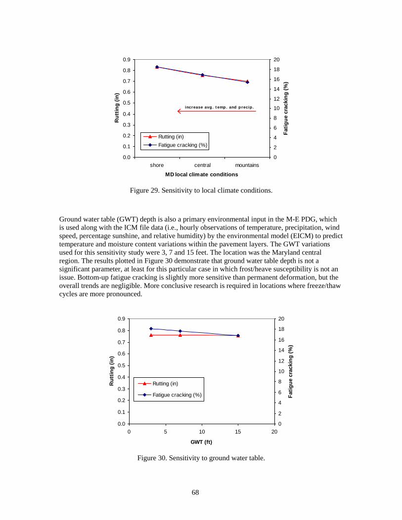
68
0.0
0.1
0.2
0.3
0.4
0.5
0.6
0.7
0.8
0.9
shore central mountains
MD local climate conditions
Ru
ttin
g (
in)
0
2
4
6
8
10
12
14
16
18
20
Fati
gu
e c
rackin
g (
%)
Rutting (in)
Fatigue cracking (%)
increase avg . t emp. and precip .
Figure 29. Sensitivity to local climate conditions.
Ground water table (GWT) depth is also a primary environmental input in the M-E PDG, which
is used along with the ICM file data (i.e., hourly observations of temperature, precipitation, wind
speed, percentage sunshine, and relative humidity) by the environmental model (EICM) to predict
temperature and moisture content variations within the pavement layers. The GWT variations
used for this sensitivity study were 3, 7 and 15 feet. The location was the Maryland central
region. The results plotted in Figure 30 demonstrate that ground water table depth is not a
significant parameter, at least for this particular case in which frost/heave susceptibility is not an
issue. Bottom-up fatigue cracking is slightly more sensitive than permanent deformation, but the
overall trends are negligible. More conclusive research is required in locations where freeze/thaw
cycles are more pronounced.
0.0
0.1
0.2
0.3
0.4
0.5
0.6
0.7
0.8
0.9
0 5 10 15 20
GWT (ft)
Ru
ttin
g (
in)
0
2
4
6
8
10
12
14
16
18
20
Fati
gu
e c
rackin
g (
%)
Rutting (in)
Fatigue cracking (%)
Figure 30. Sensitivity to ground water table.
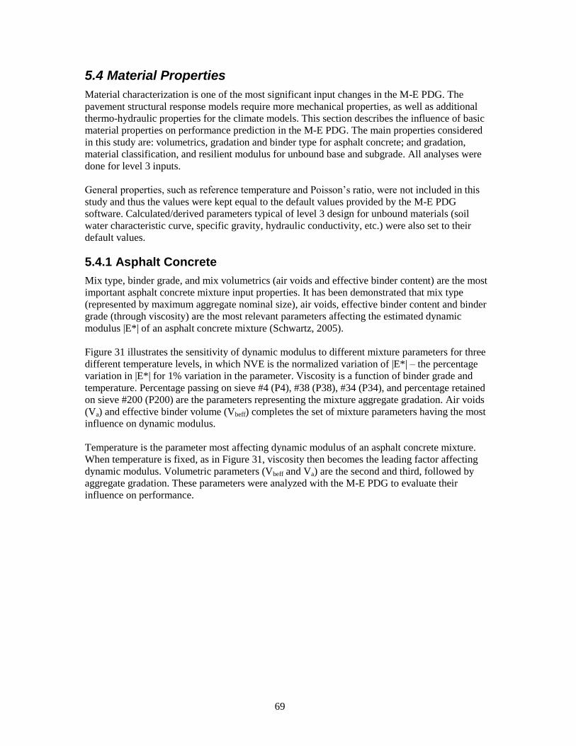
69
5.4 Material Properties
Material characterization is one of the most significant input changes in the M-E PDG. The
pavement structural response models require more mechanical properties, as well as additional
thermo-hydraulic properties for the climate models. This section describes the influence of basic
material properties on performance prediction in the M-E PDG. The main properties considered
in this study are: volumetrics, gradation and binder type for asphalt concrete; and gradation,
material classification, and resilient modulus for unbound base and subgrade. All analyses were
done for level 3 inputs.
General properties, such as reference temperature and Poisson’s ratio, were not included in this
study and thus the values were kept equal to the default values provided by the M-E PDG
software. Calculated/derived parameters typical of level 3 design for unbound materials (soil
water characteristic curve, specific gravity, hydraulic conductivity, etc.) were also set to their
default values.
5.4.1 Asphalt Concrete
Mix type, binder grade, and mix volumetrics (air voids and effective binder content) are the most
important asphalt concrete mixture input properties. It has been demonstrated that mix type
(represented by maximum aggregate nominal size), air voids, effective binder content and binder
grade (through viscosity) are the most relevant parameters affecting the estimated dynamic
modulus |E*| of an asphalt concrete mixture (Schwartz, 2005).
Figure 31 illustrates the sensitivity of dynamic modulus to different mixture parameters for three
different temperature levels, in which NVE is the normalized variation of |E*| – the percentage
variation in |E*| for 1% variation in the parameter. Viscosity is a function of binder grade and
temperature. Percentage passing on sieve #4 (P4), #38 (P38), #34 (P34), and percentage retained
on sieve #200 (P200) are the parameters representing the mixture aggregate gradation. Air voids
(Va) and effective binder volume (Vbeff) completes the set of mixture parameters having the most
influence on dynamic modulus.
Temperature is the parameter most affecting dynamic modulus of an asphalt concrete mixture.
When temperature is fixed, as in Figure 31, viscosity then becomes the leading factor affecting
dynamic modulus. Volumetric parameters (Vbeff and Va) are the second and third, followed by
aggregate gradation. These parameters were analyzed with the M-E PDG to evaluate their
influence on performance.
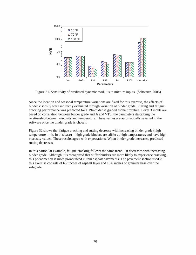
70
0.0
0.1
1.0
10.0
100.0
Va Vbeff P34 P38 P4 P200 Viscosity
Parameters
NV
E
10 °F
70 °F
130 °F
Figure 31. Sensitivity of predicted dynamic modulus to mixture inputs. (Schwartz, 2005)
Since the location and seasonal temperature variations are fixed for this exercise, the effects of
binder viscosity were indirectly evaluated through variation of binder grade. Rutting and fatigue
cracking performance was predicted for a 19mm dense graded asphalt mixture. Level 3 inputs are
based on correlation between binder grade and A and VTS, the parameters describing the
relationship between viscosity and temperature. These values are automatically selected in the
software once the binder grade is chosen.
Figure 32 shows that fatigue cracking and rutting decrease with increasing binder grade (high
temperature limit, in this case) – high grade binders are stiffer at high temperatures and have high
viscosity values. These results agree with expectations. When binder grade increases, predicted
rutting decreases.
In this particular example, fatigue cracking follows the same trend – it decreases with increasing
binder grade. Although it is recognized that stiffer binders are more likely to experience cracking,
this phenomenon is more pronounced in thin asphalt pavements. The pavement section used in
this exercise consists of 6.7 inches of asphalt layer and 18.6 inches of granular base over the
subgrade.
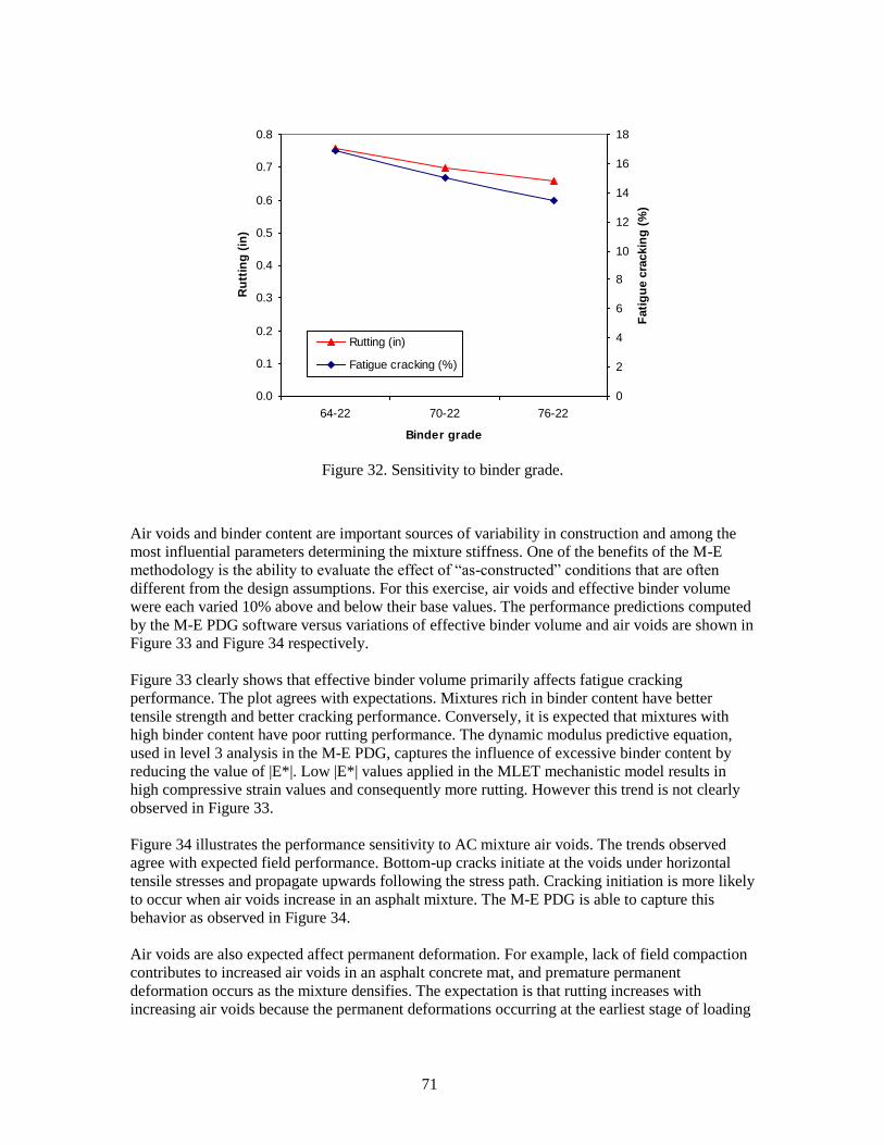
71
0.0
0.1
0.2
0.3
0.4
0.5
0.6
0.7
0.8
64-22 70-22 76-22
Binder grade
Ru
ttin
g (
in)
0
2
4
6
8
10
12
14
16
18
Fati
gu
e c
rackin
g (
%)
Rutting (in)
Fatigue cracking (%)
Figure 32. Sensitivity to binder grade.
Air voids and binder content are important sources of variability in construction and among the
most influential parameters determining the mixture stiffness. One of the benefits of the M-E
methodology is the ability to evaluate the effect of ―as-constructed‖ conditions that are often
different from the design assumptions. For this exercise, air voids and effective binder volume
were each varied 10% above and below their base values. The performance predictions computed
by the M-E PDG software versus variations of effective binder volume and air voids are shown in
Figure 33 and Figure 34 respectively.
Figure 33 clearly shows that effective binder volume primarily affects fatigue cracking
performance. The plot agrees with expectations. Mixtures rich in binder content have better
tensile strength and better cracking performance. Conversely, it is expected that mixtures with
high binder content have poor rutting performance. The dynamic modulus predictive equation,
used in level 3 analysis in the M-E PDG, captures the influence of excessive binder content by
reducing the value of |E*|. Low |E*| values applied in the MLET mechanistic model results in
high compressive strain values and consequently more rutting. However this trend is not clearly
observed in Figure 33.
Figure 34 illustrates the performance sensitivity to AC mixture air voids. The trends observed
agree with expected field performance. Bottom-up cracks initiate at the voids under horizontal
tensile stresses and propagate upwards following the stress path. Cracking initiation is more likely
to occur when air voids increase in an asphalt mixture. The M-E PDG is able to capture this
behavior as observed in Figure 34.
Air voids are also expected affect permanent deformation. For example, lack of field compaction
contributes to increased air voids in an asphalt concrete mat, and premature permanent
deformation occurs as the mixture densifies. The expectation is that rutting increases with
increasing air voids because the permanent deformations occurring at the earliest stage of loading
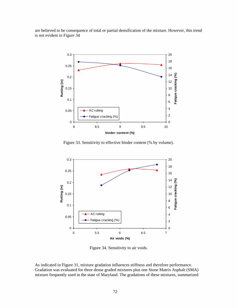
72
are believed to be consequence of total or partial densification of the mixture. However, this trend
is not evident in Figure 34
0
0.05
0.1
0.15
0.2
0.25
0.3
8 8.5 9 9.5 10
binder content (%)
Ru
ttin
g (
in)
0
2
4
6
8
10
12
14
16
18
20
Fati
gu
e c
rackin
g (
%)
AC rutting
Fatigue cracking (%)
Figure 33. Sensitivity to effective binder content (% by volume).
0
0.05
0.1
0.15
0.2
0.25
0.3
5 5.5 6 6.5 7
Air voids (%)
Ru
ttin
g (
in)
0
2
4
6
8
10
12
14
16
18
20
Fati
gu
e c
rackin
g (
%)
AC rutting
Fatigue cracking (%)
Figure 34. Sensitivity to air voids.
As indicated in Figure 31, mixture gradation influences stiffness and therefore performance.
Gradation was evaluated for three dense graded mixtures plus one Stone Matrix Asphalt (SMA)
mixture frequently used in the state of Maryland. The gradations of these mixtures, summarized
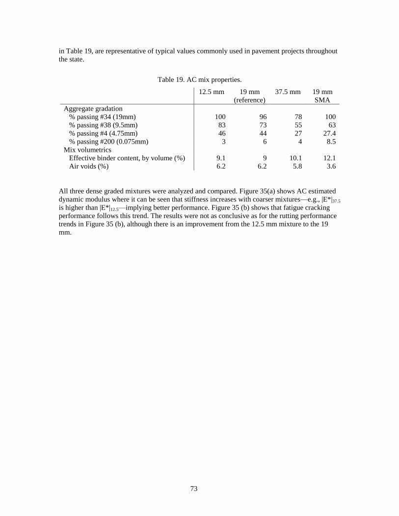
73
in Table 19, are representative of typical values commonly used in pavement projects throughout
the state.
Table 19. AC mix properties.
12.5 mm 19 mm
(reference)
37.5 mm 19 mm
SMA
Aggregate gradation
% passing #34 (19mm) 100 96 78 100
% passing #38 (9.5mm) 83 73 55 63
% passing #4 (4.75mm) 46 44 27 27.4
% passing #200 (0.075mm) 3 6 4 8.5
Mix volumetrics
Effective binder content, by volume (%) 9.1 9 10.1 12.1
Air voids (%) 6.2 6.2 5.8 3.6
All three dense graded mixtures were analyzed and compared. Figure 35(a) shows AC estimated
dynamic modulus where it can be seen that stiffness increases with coarser mixtures—e.g., |E*|37.5
is higher than |E*|12.5—implying better performance. Figure 35 (b) shows that fatigue cracking
performance follows this trend. The results were not as conclusive as for the rutting performance
trends in Figure 35 (b), although there is an improvement from the 12.5 mm mixture to the 19
mm.
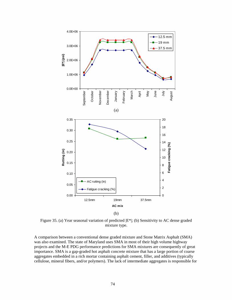
74
0.0E+00
1.0E+06
2.0E+06
3.0E+06
4.0E+06
Septe
mber
Octo
ber
Novem
ber
Decem
ber
January
Febru
ary
Marc
h
April
May
June
July
August
|E*|
(p
si)
12.5 mm
19 mm
37.5 mm
(a)
0.00
0.05
0.10
0.15
0.20
0.25
0.30
0.35
12.5mm 19mm 37.5mm
AC mix
Ru
ttin
g (
in)
0
2
4
6
8
10
12
14
16
18
20
Fati
gu
e c
rackin
g (
%)
AC rutting (in)
Fatigue cracking (%)
(b)
Figure 35. (a) Year seasonal variation of predicted |E*|; (b) Sensitivity to AC dense graded
mixture type.
A comparison between a conventional dense graded mixture and Stone Matrix Asphalt (SMA)
was also examined. The state of Maryland uses SMA in most of their high volume highway
projects and the M-E PDG performance predictions for SMA mixtures are consequently of great
importance. SMA is a gap-graded hot asphalt concrete mixture that has a large portion of coarse
aggregates embedded in a rich mortar containing asphalt cement, filler, and additives (typically
cellulose, mineral fibers, and/or polymers). The lack of intermediate aggregates is responsible for

75
forming a stone-on-stone aggregate contact that provides strength, durability and rutting
resistance (Brown and Cooley, 1999; Michael et al., 2003).
Examples of SMA’s exceptional rutting performance can be found in the literature. Michael et al.
(2003) summarized typical rutting performance of 86 Maryland projects in service, with ages
varying from 1 to 9 years, where measured total rut depth ranged from 0.05 to 0.20 inches – a
good indication of SMA’s rut-resistance. However, when SMA is analyzed using the M-E PDG
its rut-resistant benefits cannot be observed. Figure 36(a) illustrates the performance of a 19mm
SMA mixture compared to an equivalent dense graded mixture. The SMA exhibits higher rutting
than dense graded mixture, which contradicts field experience. Figure 36 (b) shows seasonal
variations of dynamic modulus for 19mm SMA and dense graded mixture. The dynamic modulus
predicted in the M-E PDG for SMA is lower than for the dense graded mixture, which is
consistent with the lower rutting predicted for the dense graded mixtures.
The dynamic modulus of SMA mixtures measured in laboratory is also lower than that of similar
dense graded mixtures. One possible reason is the dynamic modulus testing protocol, in which the
specimen is tested in unconfined conditions. Gap-graded mixtures like SMA depend more upon
aggregate interlock derived from the stone-on-stone contact and as a consequence some
researchers claim that testing under confined conditions is necessary to reflect realistically the
true stiffness and strength of the material. The |E*| predictive model also has problems, as the
database used for the model calibration includes only dense graded mixtures.
The principal conclusion drawn from this exercise is that the M-E PDG procedure in its present
form cannot realistically predict the rutting performance of SMA mixtures. Continuing research
on this subject includes the just-started NCHRP Project 9-30A to focus on improving the asphalt
concrete rutting model in the M-E PDG.
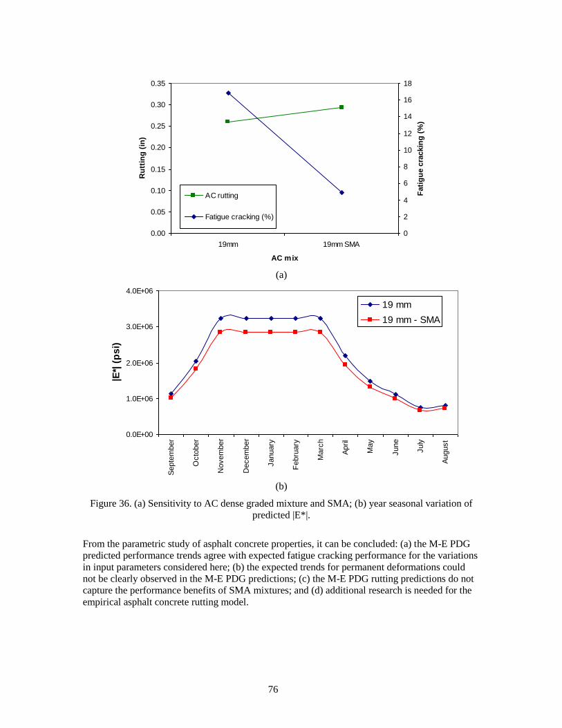
76
0.00
0.05
0.10
0.15
0.20
0.25
0.30
0.35
19mm 19mm SMA
AC mix
Ru
ttin
g (
in)
0
2
4
6
8
10
12
14
16
18
Fati
gu
e c
rackin
g (
%)
AC rutting
Fatigue cracking (%)
(a)
0.0E+00
1.0E+06
2.0E+06
3.0E+06
4.0E+06
Septe
mber
Octo
ber
Novem
ber
Decem
ber
January
Febru
ary
Marc
h
April
May
June
July
August
|E*|
(p
si)
19 mm
19 mm - SMA
(b)
Figure 36. (a) Sensitivity to AC dense graded mixture and SMA; (b) year seasonal variation of
predicted |E*|.
From the parametric study of asphalt concrete properties, it can be concluded: (a) the M-E PDG
predicted performance trends agree with expected fatigue cracking performance for the variations
in input parameters considered here; (b) the expected trends for permanent deformations could
not be clearly observed in the M-E PDG predictions; (c) the M-E PDG rutting predictions do not
capture the performance benefits of SMA mixtures; and (d) additional research is needed for the
empirical asphalt concrete rutting model.
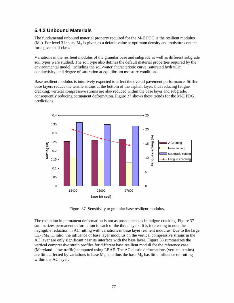
77
5.4.2 Unbound Materials
The fundamental unbound material property required for the M-E PDG is the resilient modulus
(MR). For level 3 inputs, MR is given as a default value at optimum density and moisture content
for a given soil class.
Variations in the resilient modulus of the granular base and subgrade as well as different subgrade
soil types were studied. The soil type also defines the default material properties required by the
environmental model, including the soil-water characteristic curve, saturated hydraulic
conductivity, and degree of saturation at equilibrium moisture conditions.
Base resilient modulus is intuitively expected to affect the overall pavement performance. Stiffer
base layers reduce the tensile strains at the bottom of the asphalt layer, thus reducing fatigue
cracking; vertical compressive strains are also reduced within the base layer and subgrade,
consequently reducing permanent deformation. Figure 37 shows these trends for the M-E PDG
predictions.
0
0.05
0.1
0.15
0.2
0.25
0.3
0.35
0.4
18400 23000 27600
Base Mr (psi)
Ru
ttin
g (
in)
0
5
10
15
20
25
Fati
gu
e c
rackin
g (
%)
AC rutting
base rutting
subgrade rutting
Fatigue cracking
Figure 37. Sensitivity to granular base resilient modulus.
The reduction in permanent deformation is not as pronounced as in fatigue cracking. Figure 37
summarizes permanent deformation in each of the three layers. It is interesting to note the
negligible reduction in AC rutting with variations in base layer resilient modulus. Due to the large
|EAC|/MR,base ratio, the influence of base layer modulus on the vertical compressive strains in the
AC layer are only significant near its interface with the base layer. Figure 38 summarizes the
vertical compressive strain profiles for different base resilient moduli for the reference case
(Maryland – low traffic) computed using LEAF. The AC elastic deformations (vertical strains)
are little affected by variations in base MR, and thus the base MR has little influence on rutting
within the AC layer.
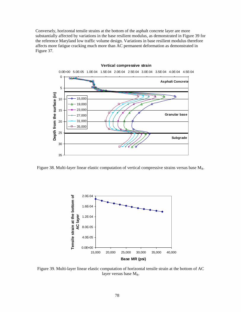
78
Conversely, horizontal tensile strains at the bottom of the asphalt concrete layer are more
substantially affected by variations in the base resilient modulus, as demonstrated in Figure 39 for
the reference Maryland low traffic volume design. Variations in base resilient modulus therefore
affects more fatigue cracking much more than AC permanent deformation as demonstrated in
Figure 37.
0
5
10
15
20
25
30
35
0.0E+00 5.0E-05 1.0E-04 1.5E-04 2.0E-04 2.5E-04 3.0E-04 3.5E-04 4.0E-04 4.5E-04
Vertical compressive strain
Dep
th f
rom
th
e s
urf
ace (
in)
15,000
19,000
23,000
27,000
31,000
35,000
Asphalt Concrete
Granular base
Subgrade
Figure 38. Multi-layer linear elastic computation of vertical compressive strains versus base MR.
0.0E+00
4.0E-05
8.0E-05
1.2E-04
1.6E-04
2.0E-04
15,000 20,000 25,000 30,000 35,000 40,000
Base MR (psi)
Ten
sil
e s
train
at
the b
ott
om
of
AC
layer
Figure 39. Multi-layer linear elastic computation of horizontal tensile strain at the bottom of AC
layer versus base MR.
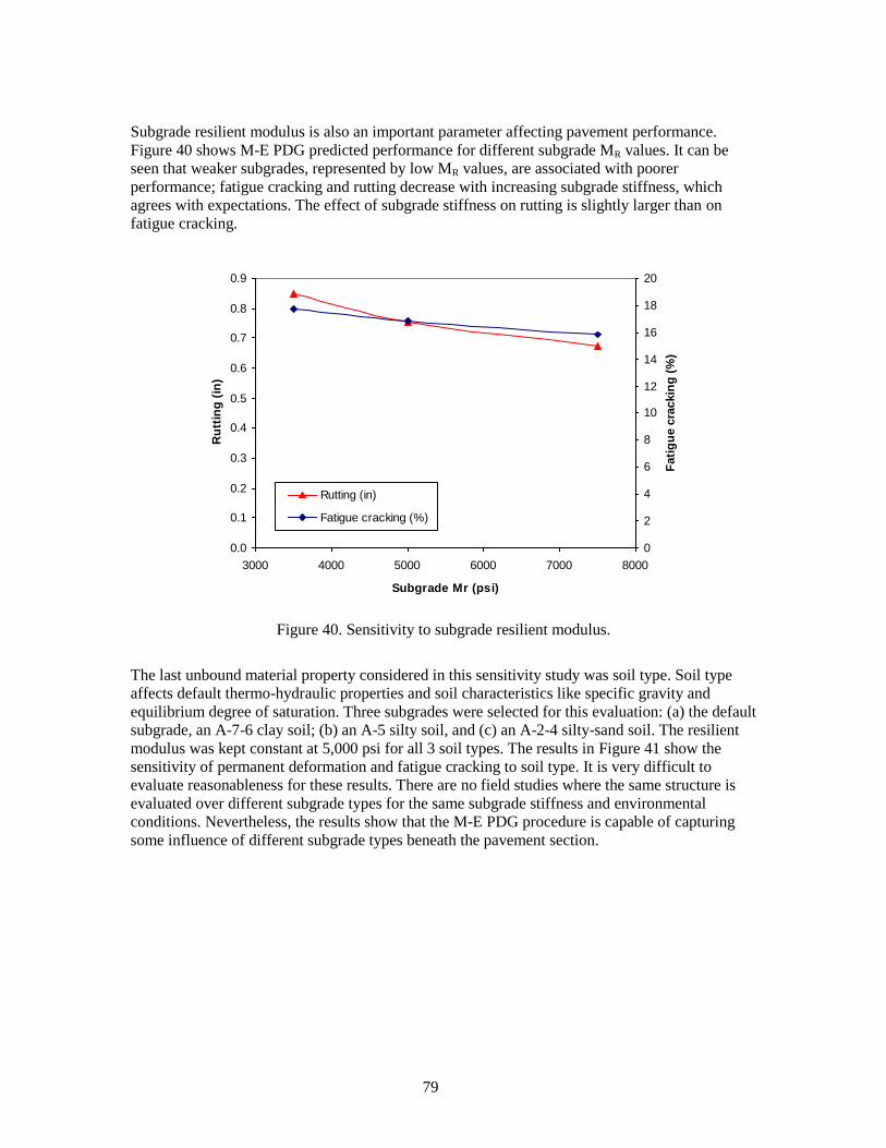
79
Subgrade resilient modulus is also an important parameter affecting pavement performance.
Figure 40 shows M-E PDG predicted performance for different subgrade MR values. It can be
seen that weaker subgrades, represented by low MR values, are associated with poorer
performance; fatigue cracking and rutting decrease with increasing subgrade stiffness, which
agrees with expectations. The effect of subgrade stiffness on rutting is slightly larger than on
fatigue cracking.
0.0
0.1
0.2
0.3
0.4
0.5
0.6
0.7
0.8
0.9
3000 4000 5000 6000 7000 8000
Subgrade Mr (psi)
Ru
ttin
g (
in)
0
2
4
6
8
10
12
14
16
18
20
Fati
gu
e c
rackin
g (
%)
Rutting (in)
Fatigue cracking (%)
Figure 40. Sensitivity to subgrade resilient modulus.
The last unbound material property considered in this sensitivity study was soil type. Soil type
affects default thermo-hydraulic properties and soil characteristics like specific gravity and
equilibrium degree of saturation. Three subgrades were selected for this evaluation: (a) the default
subgrade, an A-7-6 clay soil; (b) an A-5 silty soil, and (c) an A-2-4 silty-sand soil. The resilient
modulus was kept constant at 5,000 psi for all 3 soil types. The results in Figure 41 show the
sensitivity of permanent deformation and fatigue cracking to soil type. It is very difficult to
evaluate reasonableness for these results. There are no field studies where the same structure is
evaluated over different subgrade types for the same subgrade stiffness and environmental
conditions. Nevertheless, the results show that the M-E PDG procedure is capable of capturing
some influence of different subgrade types beneath the pavement section.
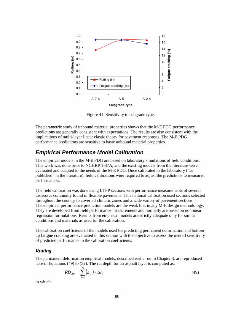
80
0.0
0.1
0.2
0.3
0.4
0.5
0.6
0.7
0.8
0.9
1.0
A-7-6 A-5 A-2-4
Subgrade type
Ru
ttin
g (
in)
0
2
4
6
8
10
12
14
16
18
Fati
gu
e c
rackin
g (
%)
Rutting (in)
Fatigue cracking (%)
Figure 41. Sensitivity to subgrade type.
The parametric study of unbound material properties shows that the M-E PDG performance
predictions are generally consistent with expectations. The results are also consistent with the
implications of multi-layer linear elastic theory for pavement responses. The M-E PDG
performance predictions are sensitive to basic unbound material properties.
Empirical Performance Model Calibration
The empirical models in the M-E PDG are based on laboratory simulations of field conditions.
This work was done prior to NCHRP 1-37A, and the existing models from the literature were
evaluated and adapted to the needs of the M-E PDG. Once calibrated in the laboratory (―as-
published‖ in the literature), field calibrations were required to adjust the predictions to measured
performances.
The field calibration was done using LTPP sections with performance measurements of several
distresses commonly found in flexible pavements. This national calibration used sections selected
throughout the country to cover all climatic zones and a wide variety of pavement sections.
The empirical performance prediction models are the weak link in any M-E design methodology.
They are developed from field performance measurements and normally are based on nonlinear
regression formulations. Results from empirical models are strictly adequate only for similar
conditions and materials as used for the calibration.
The calibration coefficients of the models used for predicting permanent deformation and bottom-
up fatigue cracking are evaluated in this section with the objective to assess the overall sensitivity
of predicted performance to the calibration coefficients.
Rutting
The permanent deformation empirical models, described earlier on in Chapter 3, are reproduced
here in Equations (49) to (52). The rut depth for an asphalt layer is computed as:
N
i
iipAC hRD1
(49)
in which:
81
RDAC = rut depth at the asphalt concrete layer
N = number of sublayers
(p)i = vertical plastic strain at mid-thickness of layer i
Δhi = thickness of sublayer i
The plastic strain within each sublayer is determined from the following empirical equation:
32 0.47911.56063.4488
3 110p
r
T N
(50)
in which:
p = vertical plastic strain at mid-thickness of sublayer i
r = computed vertical resilient strain at mid-thickness of sublayer i for a given load
σ3 = function of total asphalt layers thickness and depth to computational point, to
correct for the confining pressure at different depths.
1, 2, 3 = field calibration coefficients
T = t emperature
N = number of repetitions for a given load
The depth correction factor is determined using the following empirical expression:
3 1 2( ) 0.328196depthC C depth ((51)a)
2
1 0.1039 2.4868 17.342AC ACC h h ((51)b)
2
2 0.0172 1.7331 27.428AC ACC h h ((51)c)
in which:
depth = depth from the pavement surface to the point of strain calculation
hAC = total thickness of the asphalt layers
The permanent deformation for the unbound base layer is determined using the following
empirical relation:
01 1.673 N
v
r
e h
(52)
in which:
= permanent deformation for sublayer i
1 = field calibration coefficient
0, , ρ = material properties (NCHRP, 2004)
r = resilient strain imposed in laboratory test to obtain the above material properties,
0, , and ρ
N = number of repetitions of a given load
v = computed vertical resilient strain at mid-thickness of sublayer i for a given load
h = thickness of sublayer i
For both asphalt and base layer models, the field national calibration values are equal to 1. They
were varied 10% above and below these values for this parametric study. Figure 42 and Figure 43
show percentage of rutting variation versus percentage of calibration coefficient variation for the
asphalt concrete and base layer calibration coefficients, respectively. Each coefficient was varied
separately from the others and the results reflect the percentage change in performance compared
to the unchanged condition.
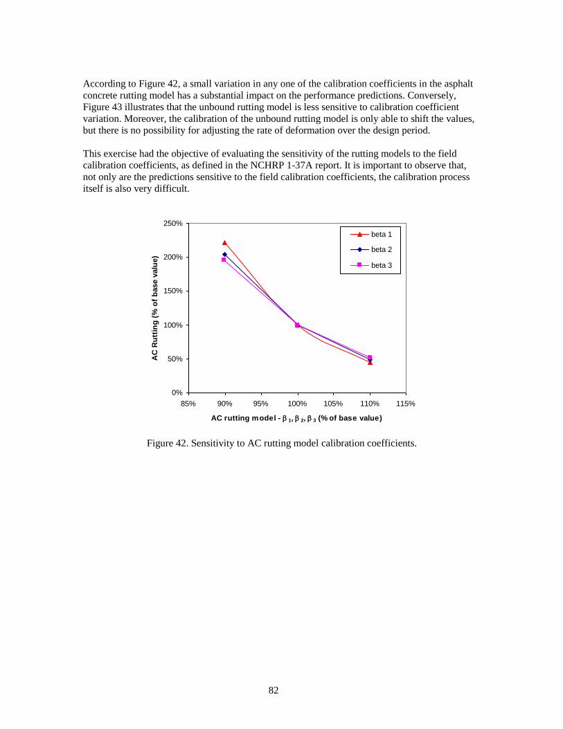
82
According to Figure 42, a small variation in any one of the calibration coefficients in the asphalt
concrete rutting model has a substantial impact on the performance predictions. Conversely,
Figure 43 illustrates that the unbound rutting model is less sensitive to calibration coefficient
variation. Moreover, the calibration of the unbound rutting model is only able to shift the values,
but there is no possibility for adjusting the rate of deformation over the design period.
This exercise had the objective of evaluating the sensitivity of the rutting models to the field
calibration coefficients, as defined in the NCHRP 1-37A report. It is important to observe that,
not only are the predictions sensitive to the field calibration coefficients, the calibration process
itself is also very difficult.
0%
50%
100%
150%
200%
250%
85% 90% 95% 100% 105% 110% 115%
AC rutting model - 1, 2, 3 (% of base value)
AC
Ru
ttin
g (
% o
f b
ase v
alu
e)
beta 1
beta 2
beta 3
Figure 42. Sensitivity to AC rutting model calibration coefficients.
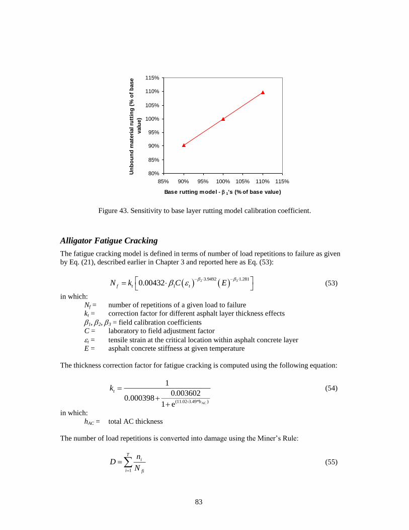
83
80%
85%
90%
95%
100%
105%
110%
115%
85% 90% 95% 100% 105% 110% 115%
Base rutting model - 1's (% of base value)
Un
bo
un
d m
ate
rial ru
ttin
g (
% o
f b
ase
valu
e)
Figure 43. Sensitivity to base layer rutting model calibration coefficient.
Alligator Fatigue Cracking
The fatigue cracking model is defined in terms of number of load repetitions to failure as given
by Eq. (21), described earlier in Chapter 3 and reported here as Eq. (53):
2 33.9492 1.281
10.00432f t tN k C E
(53)
in which:
Nf = number of repetitions of a given load to failure
kt = correction factor for different asphalt layer thickness effects
1, 2, 3 = field calibration coefficients
C = laboratory to field adjustment factor
t = tensile strain at the critical location within asphalt concrete layer
E = asphalt concrete stiffness at given temperature
The thickness correction factor for fatigue cracking is computed using the following equation:
AC(11.02-3.49*h )
1
0.0036020.000398
1 e
tk
(54)
in which:
hAC = total AC thickness
The number of load repetitions is converted into damage using the Miner’s Rule:
T
i fi
i
N
nD
1
(55)

84
in which:
D = damage
T = total number of seasonal periods
ni = actual traffic for period i
Nfi = traffic repetitions of a given load to cause failure at period i
And finally damage is converted into cracking area using the following equation:
60
1
1100log''
4
2211 DCCCCe
CFC (56)a
856.2
2 1748.3940874.2'
AChC (56)b
'
2
'
1 2CC (56)c
in which:
FC = ―alligator‖ fatigue cracking (% of total lane area)
C1, C2, C4 = constants
D = damage
hAC = total AC thickness
The fatigue model in its current configuration can only be calibrated through Eq. (53). The
coefficients 1, 2, and 3 were varied 10% above and below the default value, which is 1 for the
national calibration.
The results in Figure 44 show percentage of fatigue cracking variation versus percentage of
calibration coefficient, and except for 1 the predictions are very sensitive to calibration
coefficients. The observed distress is fatigue cracking expressed as a percentage of total lane area,
and the calibration is done on the number of loads to failure – Eq. (53). This calibration process
requires an optimization algorithm to obtain satisfactory results.
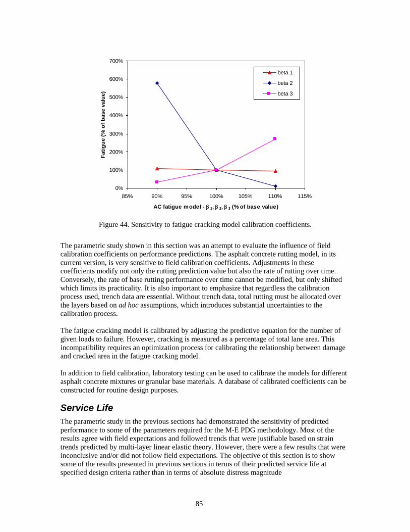
85
0%
100%
200%
300%
400%
500%
600%
700%
85% 90% 95% 100% 105% 110% 115%
AC fatigue model - 1, 2, 3 (% of base value)
Fati
gu
e (
% o
f b
ase v
alu
e)
beta 1
beta 2
beta 3
Figure 44. Sensitivity to fatigue cracking model calibration coefficients.
The parametric study shown in this section was an attempt to evaluate the influence of field
calibration coefficients on performance predictions. The asphalt concrete rutting model, in its
current version, is very sensitive to field calibration coefficients. Adjustments in these
coefficients modify not only the rutting prediction value but also the rate of rutting over time.
Conversely, the rate of base rutting performance over time cannot be modified, but only shifted
which limits its practicality. It is also important to emphasize that regardless the calibration
process used, trench data are essential. Without trench data, total rutting must be allocated over
the layers based on ad hoc assumptions, which introduces substantial uncertainties to the
calibration process.
The fatigue cracking model is calibrated by adjusting the predictive equation for the number of
given loads to failure. However, cracking is measured as a percentage of total lane area. This
incompatibility requires an optimization process for calibrating the relationship between damage
and cracked area in the fatigue cracking model.
In addition to field calibration, laboratory testing can be used to calibrate the models for different
asphalt concrete mixtures or granular base materials. A database of calibrated coefficients can be
constructed for routine design purposes.
Service Life
The parametric study in the previous sections had demonstrated the sensitivity of predicted
performance to some of the parameters required for the M-E PDG methodology. Most of the
results agree with field expectations and followed trends that were justifiable based on strain
trends predicted by multi-layer linear elastic theory. However, there were a few results that were
inconclusive and/or did not follow field expectations. The objective of this section is to show
some of the results presented in previous sections in terms of their predicted service life at
specified design criteria rather than in terms of absolute distress magnitude
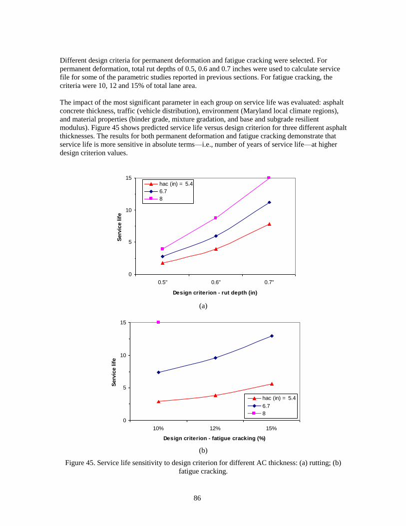
86
Different design criteria for permanent deformation and fatigue cracking were selected. For
permanent deformation, total rut depths of 0.5, 0.6 and 0.7 inches were used to calculate service
file for some of the parametric studies reported in previous sections. For fatigue cracking, the
criteria were 10, 12 and 15% of total lane area.
The impact of the most significant parameter in each group on service life was evaluated: asphalt
concrete thickness, traffic (vehicle distribution), environment (Maryland local climate regions),
and material properties (binder grade, mixture gradation, and base and subgrade resilient
modulus). Figure 45 shows predicted service life versus design criterion for three different asphalt
thicknesses. The results for both permanent deformation and fatigue cracking demonstrate that
service life is more sensitive in absolute terms—i.e., number of years of service life—at higher
design criterion values.
0
5
10
15
0.5'' 0.6'' 0.7''
Design criterion - rut depth (in)
Serv
ice lif
e
hac (in) = 5.4
6.7
8
(a)
0
5
10
15
10% 12% 15%
Design criterion - fatigue cracking (%)
Serv
ice lif
e
hac (in) = 5.4
6.7
8
(b)
Figure 45. Service life sensitivity to design criterion for different AC thickness: (a) rutting; (b)
fatigue cracking.
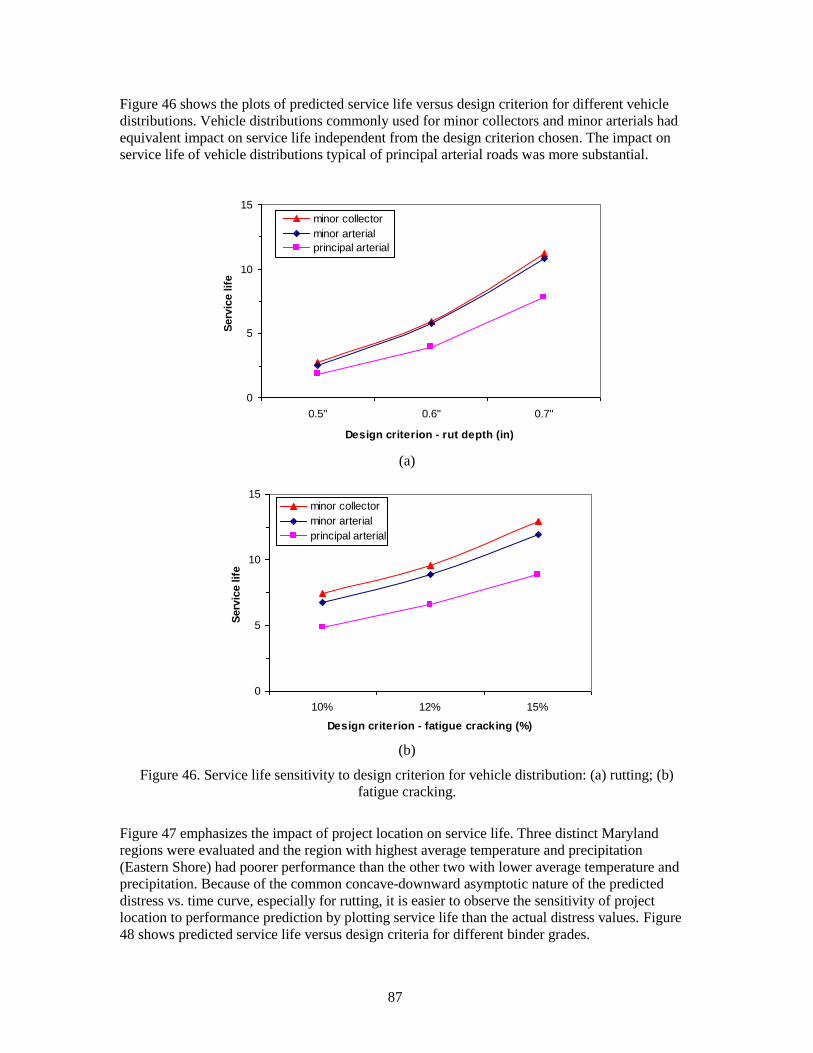
87
Figure 46 shows the plots of predicted service life versus design criterion for different vehicle
distributions. Vehicle distributions commonly used for minor collectors and minor arterials had
equivalent impact on service life independent from the design criterion chosen. The impact on
service life of vehicle distributions typical of principal arterial roads was more substantial.
0
5
10
15
0.5'' 0.6'' 0.7''
Design criterion - rut depth (in)
Serv
ice lif
eminor collector
minor arterial
principal arterial
(a)
0
5
10
15
10% 12% 15%
Design criterion - fatigue cracking (%)
Serv
ice lif
e
minor collector
minor arterial
principal arterial
(b)
Figure 46. Service life sensitivity to design criterion for vehicle distribution: (a) rutting; (b)
fatigue cracking.
Figure 47 emphasizes the impact of project location on service life. Three distinct Maryland
regions were evaluated and the region with highest average temperature and precipitation
(Eastern Shore) had poorer performance than the other two with lower average temperature and
precipitation. Because of the common concave-downward asymptotic nature of the predicted
distress vs. time curve, especially for rutting, it is easier to observe the sensitivity of project
location to performance prediction by plotting service life than the actual distress values. Figure
48 shows predicted service life versus design criteria for different binder grades.
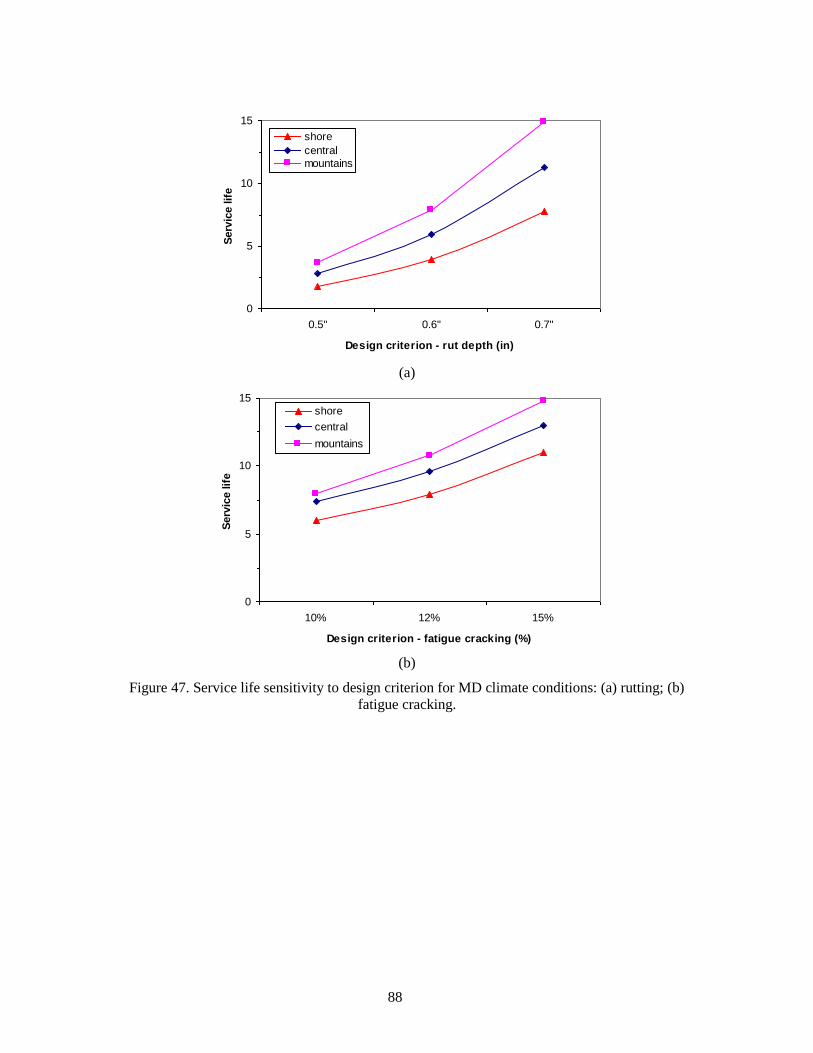
88
0
5
10
15
0.5'' 0.6'' 0.7''
Design criterion - rut depth (in)
Serv
ice lif
e
shore
central
mountains
(a)
0
5
10
15
10% 12% 15%
Design criterion - fatigue cracking (%)
Serv
ice lif
e
shore
central
mountains
(b)
Figure 47. Service life sensitivity to design criterion for MD climate conditions: (a) rutting; (b)
fatigue cracking.
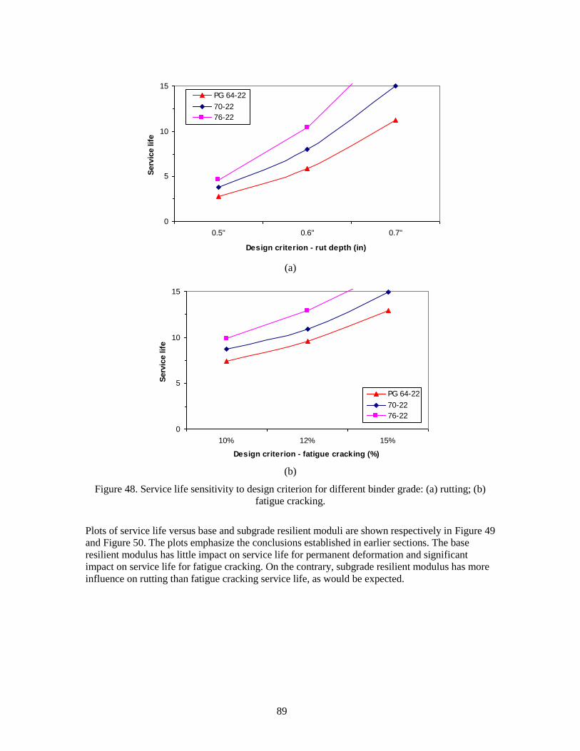
89
0
5
10
15
0.5'' 0.6'' 0.7''
Design criterion - rut depth (in)
Serv
ice lif
e
PG 64-22
70-22
76-22
(a)
0
5
10
15
10% 12% 15%
Design criterion - fatigue cracking (%)
Serv
ice lif
e
PG 64-22
70-22
76-22
(b)
Figure 48. Service life sensitivity to design criterion for different binder grade: (a) rutting; (b)
fatigue cracking.
Plots of service life versus base and subgrade resilient moduli are shown respectively in Figure 49
and Figure 50. The plots emphasize the conclusions established in earlier sections. The base
resilient modulus has little impact on service life for permanent deformation and significant
impact on service life for fatigue cracking. On the contrary, subgrade resilient modulus has more
influence on rutting than fatigue cracking service life, as would be expected.
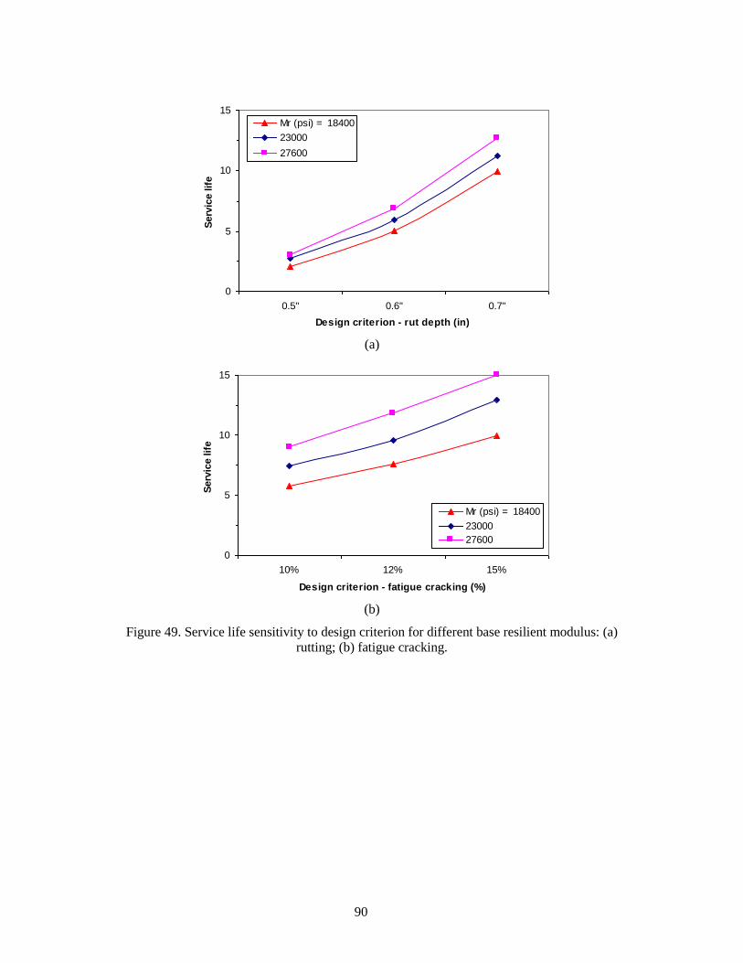
90
0
5
10
15
0.5'' 0.6'' 0.7''
Design criterion - rut depth (in)
Serv
ice lif
e
Mr (psi) = 18400
23000
27600
(a)
0
5
10
15
10% 12% 15%
Design criterion - fatigue cracking (%)
Serv
ice lif
e
Mr (psi) = 18400
23000
27600
(b)
Figure 49. Service life sensitivity to design criterion for different base resilient modulus: (a)
rutting; (b) fatigue cracking.
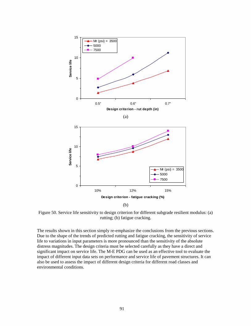
91
0
5
10
15
0.5'' 0.6'' 0.7''
Design criterion - rut depth (in)
Serv
ice lif
e
Mr (psi) = 3500
5000
7500
(a)
0
5
10
15
10% 12% 15%
Design criterion - fatigue cracking (%)
Serv
ice lif
e
Mr (psi) = 3500
5000
7500
(b)
Figure 50. Service life sensitivity to design criterion for different subgrade resilient modulus: (a)
rutting; (b) fatigue cracking.
The results shown in this section simply re-emphasize the conclusions from the previous sections.
Due to the shape of the trends of predicted rutting and fatigue cracking, the sensitivity of service
life to variations in input parameters is more pronounced than the sensitivity of the absolute
distress magnitudes. The design criteria must be selected carefully as they have a direct and
significant impact on service life. The M-E PDG can be used as an effective tool to evaluate the
impact of different input data sets on performance and service life of pavement structures. It can
also be used to assess the impact of different design criteria for different road classes and
environmental conditions.
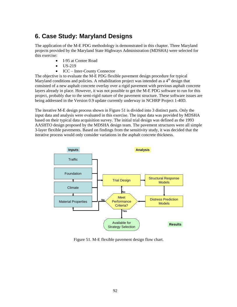
92
6. Case Study: Maryland Designs
The application of the M-E PDG methodology is demonstrated in this chapter. Three Maryland
projects provided by the Maryland State Highways Administration (MDSHA) were selected for
this exercise:
I-95 at Contee Road
US-219
ICC – Inter-County Connector
The objective is to evaluate the M-E PDG flexible pavement design procedure for typical
Maryland conditions and policies. A rehabilitation project was intended as a 4th design that
consisted of a new asphalt concrete overlay over a rigid pavement with previous asphalt concrete
layers already in place. However, it was not possible to get the M-E PDG software to run for this
project, probably due to the semi-rigid nature of the pavement structure. These software issues are
being addressed in the Version 0.9 update currently underway in NCHRP Project 1-40D.
The iterative M-E design process shown in Figure 51 is divided into 3 distinct parts. Only the
input data and analysis were evaluated in this exercise. The input data was provided by MDSHA
based on their typical data acquisition survey. The initial trial design was defined as the 1993
AASHTO design proposed by the MDSHA design team. The pavement structures were all simple
3-layer flexible pavements. Based on findings from the sensitivity study, it was decided that the
iterative process would only consider variations in the asphalt concrete thickness.
Traffic
Foundation
Climate
Material Properties
Trial DesignStructural Response
Models
Distress Prediction
Models
Meet
Performance
Criteria?
Available for
Strategy Selection
Yes
No
No
InputsInputs AnalysisAnalysis
Results
Traffic
Foundation
Climate
Material Properties
Trial DesignStructural Response
Models
Distress Prediction
Models
Meet
Performance
Criteria?
Available for
Strategy Selection
Yes
No
No
InputsInputs AnalysisAnalysis
Results
Figure 51. M-E flexible pavement design flow chart.

93
6.1 Design Inputs
6.1.1 Traffic
Traffic data was provided for all three projects. The I-95 and US-219 projects are expansions of
existing alignments and therefore traffic data specifically for these projects were available. The
ICC project is a new alignment; measured traffic data was therefore not available. The MDSHA
provided their best estimates of traffic distribution and growth for the ICC project.
Traffic information included: annual average daily truck traffic (AADTT), trucks in design
direction and lane, operational speed, and traffic growth. For the projects with measured data
availability, AADTT was obtained from Automated Vehicle Classification (AVC). MDSHA
default values were used for percentage of trucks in the design direction and lane. The operational
speed was adopted as the design operational speed for the project. Table 20 presents the general
traffic inputs for the three projects.
Table 20. Traffic data for case study.
I-95 US-219 ICC
AADTT 5781 864 7362
Trucks in design direction (%) 50 50 50
Trucks in design lane (%) 80 90 80
Operational speed (mph) 60 60 65
Traffic growth (%) 1.15 2.49 0.07
Weigh-in-motion (WIM) data were provided by MDSHA for all three projects. Vehicle class and
load distributions were extracted from WIM data. In the case of the ICC project, a WIM station
close to the project location was used as reference for the typical load distribution expected for
the traffic in that region. The vehicle class distribution for the ICC project was chosen as the
default distribution for principal arterials provided in the M-E PDG. Hourly truck distribution was
only available for the US-219 project. For the I-95 and ICC projects, the M-E PDG default values
were used instead.
Figure 52 summarizes the vehicle class distribution for the three projects. Since the WIM data
were collected for a limited period of time, the load distributions were assumed to be constant
throughout the year. Figure 53 to Figure 55 show the load distribution input for each project.
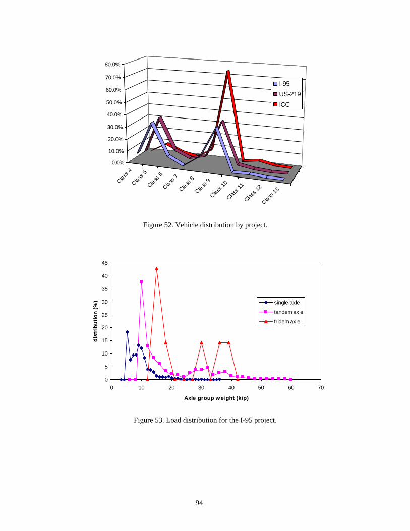
94
Cla
ss 4
Cla
ss 5
Cla
ss 6
Cla
ss 7
Cla
ss 8
Cla
ss 9
Cla
ss 1
0
Cla
ss 1
1
Cla
ss 1
2
Cla
ss 1
3
0.0%
10.0%
20.0%
30.0%
40.0%
50.0%
60.0%
70.0%
80.0%
I-95
US-219
ICC
Figure 52. Vehicle distribution by project.
0
5
10
15
20
25
30
35
40
45
0 10 20 30 40 50 60 70
Axle group weight (kip)
dis
trib
uti
on
(%
) single axle
tandem axle
tridem axle
Figure 53. Load distribution for the I-95 project.
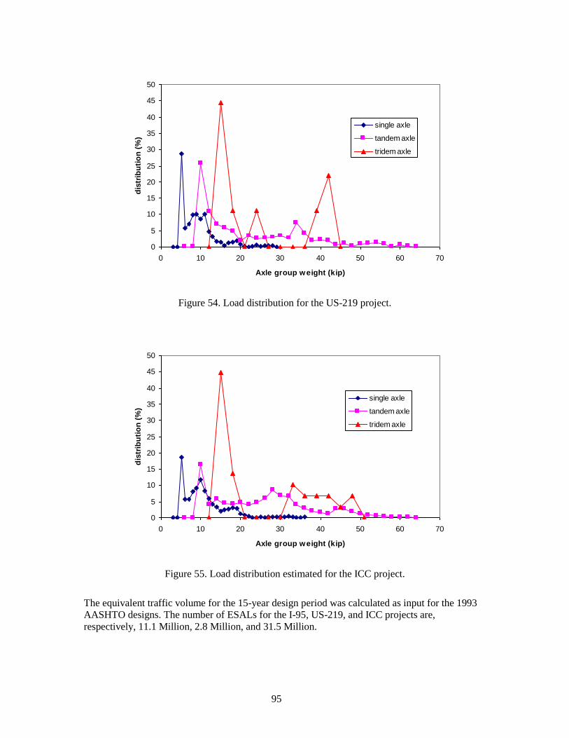
95
0
5
10
15
20
25
30
35
40
45
50
0 10 20 30 40 50 60 70
Axle group weight (kip)
dis
trib
uti
on
(%
)
single axle
tandem axle
tridem axle
Figure 54. Load distribution for the US-219 project.
0
5
10
15
20
25
30
35
40
45
50
0 10 20 30 40 50 60 70
Axle group weight (kip)
dis
trib
uti
on
(%
)
single axle
tandem axle
tridem axle
Figure 55. Load distribution estimated for the ICC project.
The equivalent traffic volume for the 15-year design period was calculated as input for the 1993
AASHTO designs. The number of ESALs for the I-95, US-219, and ICC projects are,
respectively, 11.1 Million, 2.8 Million, and 31.5 Million.

96
6.1.2 Structure and Material Properties
All three projects were designed to have the same type of structure: a three-layer flexible
pavement system consisting of asphalt concrete surface (AC), granular aggregate base (GAB),
and subgrade. The AC and GAB material properties were assumed the same in all projects for
simplification and equal to the properties used in the Maryland case presented in the comparison
study in section 4.2. Only the subgrade resilient modulus varied from project to project based on
data provided by MDSHA:
I-95 at Contee Road Mr = 7,500 psi
US-219 Mr = 5,000 psi
ICC – Inter-County Connector Mr = 5,000 psi
6.1.3 Environmental Conditions
Three integrated climate model files were generated based on global coordinates of the three
projects. The Enhanced Integrated Climate Model (EICM) interpolates climate data from weather
stations near the location of the project. The ground water table depth was assumed to be 15 ft.
6.1.4 Reliability and Performance Criteria
The reliability level for all projects was set at 95% to be consistent to what was used for the 1993
AASHTO designs provided by MDSHA. Permanent deformation and ―alligator‖ fatigue cracking
were evaluated. The other predicted distresses did not show any significant level of predicted
deterioration and were not considered.
Fatigue cracking predictions were very low, varying from 1 to 5% of the total lane area. The
fatigue cracking design criterion recommended by the M-E PDG is 25%. Permanent deformation
was the controlling distress for all the designs. The rutting design criterion recommended by the
M-E PDG is 0.75 inches. Two alternative rutting design criteria were considered in this study, 0.5
and 0.6 inches.
6.2 Designs
The 1993 AASHTO designs provided by MDSHA for the three projects were as follows:
I-95 at Contee Road
o Asphalt concrete: 12 inches
o Granular base: 12 inches
US-219
o Asphalt concrete: 9 inches
o Granular base: 18 inches
ICC
o Asphalt concrete: 15 inches
o Granular base: 15 inches
The state of Maryland has been using Stone Matrix Asphalt (SMA) in its projects for a long time.
In all three projects studied, MDSHA designed the upper 2 inches of the asphalt concrete to be a
SMA mixture. As previously discussed, the M-E PDG is not able to fully capture the benefits of
gap-graded mixtures in its current formulation. The alternative adopted to overcome this
limitation was to consider the asphalt concrete layer as a full 19mm dense mixture with the same
binder grade normally used with SMA mixtures in Maryland (PG 76-22).
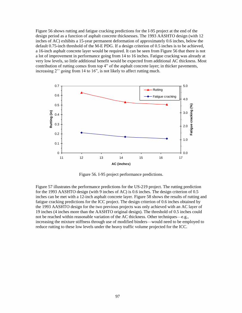
97
Figure 56 shows rutting and fatigue cracking predictions for the I-95 project at the end of the
design period as a function of asphalt concrete thicknesses. The 1993 AASHTO design (with 12
inches of AC) exhibits a 15-year permanent deformation of approximately 0.6 inches, below the
default 0.75-inch threshold of the M-E PDG. If a design criterion of 0.5 inches is to be achieved,
a 16-inch asphalt concrete layer would be required. It can be seen from Figure 56 that there is not
a lot of improvement in performance going from 14 to 16 inches. Fatigue cracking was already at
very low levels, so little additional benefit would be expected from additional AC thickness. Most
contribution of rutting comes from top 4‖ of the asphalt concrete layer; in thicker pavements,
increasing 2’’ going from 14 to 16‖, is not likely to affect rutting much.
0
0.1
0.2
0.3
0.4
0.5
0.6
0.7
11 12 13 14 15 16 17
AC (inches)
Ru
ttin
g (
in)
0.0
1.0
2.0
3.0
4.0
5.0
Fati
gu
e c
rackin
g (
%)
Rutting
Fatigue cracking
Figure 56. I-95 project performance predictions.
Figure 57 illustrates the performance predictions for the US-219 project. The rutting prediction
for the 1993 AASHTO design (with 9 inches of AC) is 0.6 inches. The design criterion of 0.5
inches can be met with a 12-inch asphalt concrete layer. Figure 58 shows the results of rutting and
fatigue cracking predictions for the ICC project. The design criterion of 0.6 inches obtained by
the 1993 AASHTO design for the two previous projects was only achieved with an AC layer of
19 inches (4 inches more than the AASHTO original design). The threshold of 0.5 inches could
not be reached within reasonable variation of the AC thickness. Other techniques—e.g.,
increasing the mixture stiffness through use of modified binders—would need to be employed to
reduce rutting to these low levels under the heavy traffic volume projected for the ICC.
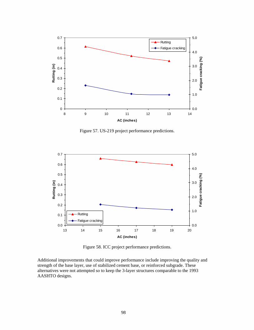
98
0
0.1
0.2
0.3
0.4
0.5
0.6
0.7
8 9 10 11 12 13 14
AC (inches)
Ru
ttin
g (
in)
0.0
1.0
2.0
3.0
4.0
5.0
Fati
gu
e c
rackin
g (
%)
Rutting
Fatigue cracking
Figure 57. US-219 project performance predictions.
0.0
0.1
0.2
0.3
0.4
0.5
0.6
0.7
13 14 15 16 17 18 19 20
AC (inches)
Ru
ttin
g (
in)
0.0
1.0
2.0
3.0
4.0
5.0
Fati
gu
e c
rackin
g (
%)
Rutting
Fatigue cracking
Figure 58. ICC project performance predictions.
Additional improvements that could improve performance include improving the quality and
strength of the base layer, use of stabilized cement base, or reinforced subgrade. These
alternatives were not attempted so to keep the 3-layer structures comparable to the 1993
AASHTO designs.
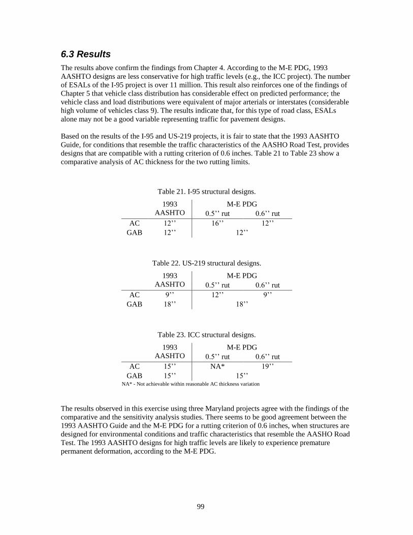
99
6.3 Results
The results above confirm the findings from Chapter 4. According to the M-E PDG, 1993
AASHTO designs are less conservative for high traffic levels (e.g., the ICC project). The number
of ESALs of the I-95 project is over 11 million. This result also reinforces one of the findings of
Chapter 5 that vehicle class distribution has considerable effect on predicted performance; the
vehicle class and load distributions were equivalent of major arterials or interstates (considerable
high volume of vehicles class 9). The results indicate that, for this type of road class, ESALs
alone may not be a good variable representing traffic for pavement designs.
Based on the results of the I-95 and US-219 projects, it is fair to state that the 1993 AASHTO
Guide, for conditions that resemble the traffic characteristics of the AASHO Road Test, provides
designs that are compatible with a rutting criterion of 0.6 inches. Table 21 to Table 23 show a
comparative analysis of AC thickness for the two rutting limits.
Table 21. I-95 structural designs.
1993
AASHTO
M-E PDG
0.5’’ rut 0.6’’ rut
AC 12’’ 16’’ 12’’
GAB 12’’ 12’’
Table 22. US-219 structural designs.
1993
AASHTO
M-E PDG
0.5’’ rut 0.6’’ rut
AC 9’’ 12’’ 9’’
GAB 18’’ 18’’
Table 23. ICC structural designs.
1993
AASHTO
M-E PDG
0.5’’ rut 0.6’’ rut
AC 15’’ NA* 19’’
GAB 15’’ 15’’ NA* - Not achievable within reasonable AC thickness variation
The results observed in this exercise using three Maryland projects agree with the findings of the
comparative and the sensitivity analysis studies. There seems to be good agreement between the
1993 AASHTO Guide and the M-E PDG for a rutting criterion of 0.6 inches, when structures are
designed for environmental conditions and traffic characteristics that resemble the AASHO Road
Test. The 1993 AASHTO designs for high traffic levels are likely to experience premature
permanent deformation, according to the M-E PDG.
100
7. Conclusions
7.1 Summary
This study has focused on comparisons between the empirical 1993 AASHTO guide and the
mechanistic-empirical pavement design guide (M-E PDG) methodology for flexible pavements
developed in NCHRP 1-37A. The comparisons were made over a span of different regions
around the country. Local input variables were obtained from a survey conducted with State
DOTs. This study also focused on analyzing the M-E PDG performance prediction sensitivity to
input parameters. The most important variables were considered in the three major groups: traffic,
environmental conditions, and material properties. A simple application of the new mechanistic-
empirical pavement design guide was also performed via evaluation of three typical pavement
projects provided by the Maryland State Highway Administration (MDSHA). Solutions from the
M-E PDG methodology were compared with 1993 AASHTO solutions. Throughout the report,
the implicit assumption is made that the M-E PDG predictions are closer to true values than those
from the 1993 AASHTO guide. All observations and conclusions are made in the context of this
assumption. The M-E PDG software version used in all calculations was the version 0.7, released
in April, 2004.
7.2 Principal Findings
The evaluations of pavement designs for different regions in the U.S. found that pavement
sections designed with the 1993 AASHTO guide for warm temperature states exhibited inferior
performance as predicted using the M-E PDG when compared to those designed for cold/mild
temperature states. This result indicates that, at least according to the M-E PDG, the 1993
AASHTO Guide overestimates the performance of pavement sections at locations having
temperatures warmer than the original AASHO Road Test site, the basis of the 1993 AASHTO
guide.
It was also found that performance predictions deteriorated consistently in all states as traffic
levels increased. These results suggest that, according to the M-E PDG, the 1993 AASHTO guide
overestimates pavement performance for traffic levels significantly beyond those experienced in
the AASHO Road Test. Traffic has always been a source of uncertainty in the 1993 AASHTO
design procedure, especially for traffic levels beyond those experienced during the AASHO Road
Test. The AASHO Road Test was trafficked with fewer than 2 million ESALs, a traffic volume
considerably lower than actual traffic on many highways today. The comparison between the
AASHTO guide and the M-E PDG procedure found that, although the pavement structures were
designed for the same serviceability loss under the 1993 AASHTO procedure, the variability of
performance predictions increased as traffic level increased when these structures were analyzed
using the M-E PDG. This result indicates that, at least according to the M-E PDG, the 1993
AASHTO designs are less reliable for high traffic and exhibit more uncertainties than those for
low traffic levels.
The parametric study of the M-E PDG provided useful and relevant insights into performance
prediction sensitivity to input parameters. Maryland design conditions at low traffic levels were
the reference case for the parametric study.
It was found that variations in base thickness had little influence on fatigue cracking and
permanent deformation. These results, although surprising from the practical application
standpoint, were found to be a direct consequence of the linear elasticity assumption for the
101
pavement materials. Due to the much higher asphalt concrete stiffness, varying the base thickness
did not affect the horizontal tensile strain at the bottom of the asphalt concrete layer that controls
fatigue cracking. There were small vertical strain reductions in the base layer, but they were
counterbalanced by the increase in thickness, which kept the total rutting fairly constant. Overall,
the current version of the M-E PDG attributes much less structural capacity contribution to the
unbound pavement layers than does the 1993 AASHTO procedure.
Variations of asphalt concrete thickness, on the other hand, were found to have a much more
significant impact on performance prediction, which agrees with field expectations. These results
suggest that, in the M-E PDG, the design process is dominated by the asphalt concrete layer.
Traffic data is a fundamental input for pavement design. The M-E PDG performance predictions
are very sensitive to traffic volume, as expected. In addition, the results from the parametric study
(Chapter 5) demonstrated the impacts that vehicle class and load distributions have on
performance. The results from the parametric study clearly show that the concept of equivalent
traffic is not adequate for representing traffic loading in the M-E PDG framework for permanent
deformation predictions. Results for fatigue cracking predictions were less sensitive to the details
of the traffic distribution, suggesting that equivalent traffic may be more suitable for this type of
distress, at least for low traffic and mild environmental conditions. A major advantage of the
more sophisticated characterization of traffic in the M-E PDG is that it can be successfully used
to evaluate the impact of overloaded trucks and seasonal traffic on performance; these insights
can be used to help define overload penalties and seasonal maximum weight limits.
The evaluation of environmental effect on performance indicated that the M-E PDG methodology
is very sensitive to climate zone. This agrees with field expectations; pavements in warm
locations typically exhibit more rutting and, to a lesser extent, more conventional fatigue cracking
than do pavements in mild/cold locations6. When within-region weather conditions were
simulated (i.e., evaluation of three geographical areas in the state of Maryland), the results
confirmed that the M-E PDG remains sensitive to local climate variations. These results agree
with expectations.
The most common input variables used to characterize asphalt concrete mixtures (i.e., binder
grade, air voids and binder content) and granular base materials (i.e., base and subgrade resilient
modulus and subgrade soil type) were also investigated in the parametric sensitivity study. The
expected fatigue cracking performance trends agree with the M-E PDG predictions for the
variations in the asphalt concrete material input parameters considered. However, the trends for
permanent deformation were not quite so clear, which is less consistent with engineering
experience. The effect of mixture volumetrics was also investigated by comparing performance
predictions for dense graded against gap-graded (i.e., Stone Matrix Asphalt) mixtures. The M-E
PDG performance predictions did not realistically capture the behavior of SMA mixtures. This is
particularly problematic for the state of Maryland, which is one of the national leaders in SMA
production and placement.
The M-E PDG fatigue cracking predictions were sensitive to the base layer resilient modulus but
relatively insensitive to subgrade resilient modulus. These results agree with physical
expectations and with the elastic theory, in which the asphalt concrete/base stiffness ratio is an
important factor defining the strain magnitude at the interface between the two layers.
Conversely, subgrade resilient modulus had more impact on permanent deformation than the base
6 Thermal cracking was not considered in this study because it is not an issue at all the locations analyzed.
Thermal cracking is important only in cold climates.
102
resilient modulus. Rutting variations with subgrade stiffness are expected; soft subgrades are
more likely to experience higher rutting levels than stiff subgrades. These results reinforce the
earlier observation that the M-E PDG is less sensitive to base layer properties than is the 1993
AASHTO procedure.
The parametric sensitivity study suggests how the M-E PDG methodology can be valuable for
determining pay factors for quality control/quality assurance programs in state agencies. As-built
construction data can be used as input data to assess post-construction performance as compared
to design expectations.
The sensitivity of performance predictions to the empirical model calibrations was also evaluated
in the parametric sensitivity study. Predicted performance was found to be very sensitive to small
variations of the permanent deformation and fatigue cracking empirical model calibration
coefficients. This result suggests the importance of local calibration of the performance prediction
models. It is expected that, even within small regions, different material types (e.g., different
asphalt concrete mixtures, subgrade soil types) may have different calibration coefficients.
The sensitivity of service life to the specified design criteria was also investigated. Due to the
concave-downward asymptotic shape of the two distress predictions evaluated, the sensitivity of
service life to variations in input parameters is quite significant. The use of tolerance levels on
acceptable service life should be considered to mitigate the effects of the shape of the prediction
models considered in here. With that being stated, it was found that the M-E PDG procedure can
be used as an effective tool to evaluate the impact of different design criteria on performance and
service life of pavement structures. This type of evaluation is useful to agencies when defining
the design criteria for different road classes and environmental conditions.
The results of the three Maryland projects agreed with the findings of the comparative and the
sensitivity studies. The 1993 AASHTO Guide provided structures that satisfied a rutting criterion
of 0.6 inches on average, based on M-E PDG predictions. Similar results were found in pavement
sections designed for low traffic and mild/cold climate conditions in the comparative study
(South Dakota and Washington State). No significant fatigue cracking was observed in any of the
three Maryland designs. This is consistent with reality; cracking is not frequently observed in
major Maryland roads, except for reflection cracking in Portland cement concrete pavements
having asphalt concrete overlays.
7.3 Implementation Issues
The implementation of the M-E PDG is a challenging task to state agencies. In addition to the
local calibration needed to enhance the effectiveness and accuracy of the empirical performance
models, large amounts of input data are required for routine designs. Traffic characterization
needs careful assessment; Automated Vehicle Counters (AVC) and Weigh-in-motion (WIM)
stations can be used to provide the data required in the M-E PDG. A database of regional load
spectra data by road functional class can be developed as an alternative to project-specific traffic
data collection, particularly for less important projects.
Material characterization inputs can also be placed in a database for use in routine designs. As
shown consistently in this study, the impact of unbound materials on performance as predicted by
the M-E PDG is less pronounced than the impact of asphalt concrete. Continuing research is
needed to better model the behavior of unbound materials in the pavement structure.
To reduce the burden of level 1 material characterization (i.e., laboratory-specific data) at early
stages of implementation, level 3 (i.e., correlated material properties or selected from range of
103
typical values) should be considered for all materials, especially for the unbound materials.
Asphalt concrete level 3 inputs are easily obtained from mixture volumetrics and gradation.
However, given the sensitivity of performance predictions to the asphalt concrete properties, level
1 characterization of typical mixes should be a high implementation priority. Improved asphalt
testing equipment (e.g., the Simple Performance Tester developed in NCHRP Project 9-29) will
make it easier for agencies to collect level 1 laboratory measured asphalt concrete dynamic
moduli in the future. Unbound resilient modulus can be estimated from material type, at least
during the early stages of implementation. For major projects and/or as more expertise is
accumulated, samples of granular base materials and subgrade can be tested in the laboratory to
determine resilient modulus at optimum density and moisture content, or field FWD data can be
used to backcalculate resilient modulus. Databases of material property inputs can be developed
for routine design applications.
Continuing research to enhance the M-E PDG empirical models is definitely required, and some
of this is already underway in NCHRP Projects 1-41 (reflection cracking), 1-42A (top-down
fatigue cracking), and 9-30A (HMA rutting). Based on engineering judgment of the
reasonableness of predictions shown in this report and predictions computed by different authors
presented in conferences over the past two years, the rutting model was considered the weakest of
the two distress models investigated in this study. The rutting model was calibrated without a full
set of appropriate field data. Trench data were not available in the LTPP database; consequently,
the distribution of rutting over the pavement layers must be estimated in the M-E PDG software
based on limited available trench data from the original AASHO Road Test, from the MnRoad
field experiment, and engineering judgment. Considerable additional research is required to
enhance the rutting model; this is currently underway in NCHRP Project 9-30A. The ideal for a
more robust rutting model is one based more rigorously on advanced theories of mechanics that
can better capture the deterioration and permanent deformation response of the asphalt concrete
and other flexible pavement materials.
104
8. References
AASHTO. (1972). AASHTO Interim Guide for Design of Pavements Structures, American
Association of State Highway and Transportation Officials, Washington, DC.
AASHTO. (1986). AASHTO Guide for Design of Pavements Structures, American Association of
State Highway and Transportation Officials, Washington, DC.
AASHTO. (1993). AASHTO Guide for Design of Pavements Structures, American Association of
State Highway and Transportation Officials, Washington, DC.
Asphalt-Institute. (1982). Reseach and Development of the Asphalt Institute's Thickness Design
Manual (MS-1), 9th ed. Research Report 82-2ts, Asphalt Institute, Lexington, KY.
Asphalt-Institute. (1991). Thickness Design - Asphalt Pavements for Highways and Streets.
Manual Series No.1 (MS-1), Asphalt Institute, Lexington, KY.
Attoh-Okine, N. O. (2002). "Uncertainty Analysis in Structural Number Determination in
Flexible Pavement Design - A Convex Model Approach," Construction and Building
Materials, Vol. 16, No. 2, pp. 67-71.
Ayres, M. (1997). Development of a Rational Probabilistic Approach for Flexible Pavement
Analysis, Ph.D. Dissertation, University of Maryland, College Park, MD.
Baladi, G. Y., and A. Thomas. (1994). "Mechanistic Evaluation of AASHTO Flexible Pavement
Design Equations," Transportation Research Record 1449, Washington, DC, pp. 72-78.
Basma, A. A., and T. I. Al-Suleiman. (1991). "Climatic Considerations in New AASHTO
Flexible Pavement Design," Journal of Transportation Engineering, Vol. 117, No. 2, pp.
210-223.
Brian, M., and D. G. Zollinger. (1995). "Sensitivity Analysis of Input Parameters for Pavement
Design and Reliability," Transportation Research Record 1482, Washington, DC, pp. 111-
122.
Claussen, A. I. M., J. M. Edwards, P. Sommer, and P. Udge. (1977). "Asphalt Pavement Design -
The Shell Method," Proceedings of the 4th International Conference on the Structural
Design of Asphalt Pavements, pp. 39-74.
Coree, B. J., and T. D. White. (1990). "AASHTO Flexible Pavement Design Method: Fact or
Fiction," Transportation Research Record 1286, Washington, DC, pp. 206-216.
El-Basyouny, M. M., M. W. Witczak, and S. El-Badawy. (2005). "Verification for the Calibrated
Permanent Deformation Models for the 2002 Design Guide," Proceedings of the Association
of Asphalt Pavement Technologists, Long Beach, CA, pp.
FHWA. (2001). "Guide to LTPP Traffic Data Collection and Processing," Federal Highway
Administration, Washington, DC.
Gharaybeh, F. A., H. R. Al-massaeid, and M. T. Obaidat. (1998). "Parametric Sensitivity Study of
the AASHTO Flexible Pavement Design Equation," Journal of the Institution of Engineers
(India), Vol. 78, No. 4, pp. 175-179.
Haas, R., W. R. Hudson, and J. Zaniewski. (1994). Modern Pavement Management, Krieger
Publishing Company, Malabar, FL.
Hajek, J. J. (1995). "General Axle Load Equivalency Factors," Transportation Research Record
1482, Washington, DC, pp. 67-78.
105
HRB. (1961). "The AASHO Road Test. Special Report 61A - The History and Description of the
Project," Highway Research Board, National Academy of Sciences - National Research
Council, Washington, DC.
HRB. (1962). "The AASHO Road Test. Report 5 - Pavement Research," Highway Research
Board, National Academy of Sciences - National Research Council, Washington, DC.
HRB. (1962). "The AASHO Road Test. Report 7 - Summary Report," Highway Research Board,
National Academy of Sciences - National Research Council, Washington, DC.
Huang, Y. H. (2004). Pavement Analysis and Design, Prentice-Hall, Upper Saddle River, NJ.
Kaloush, K. E. (2001). Simple Performance Test for Permanent Deformation of Asphalt Mixtures,
Ph.D. Dissertation, Arizona State University, Tempe, AZ.
Kansas-State-Highway-Commision. (1947). "Design of Flexible Pavement Using the Triaxial
Compression Test," Highway Research Board, Vol. Bulletin 8, No., pp.
Lavin, P. (2003). Asphalt Pavements, Spon Press, New York, NY.
Leahy, R. B. (1989). Permanent Deformation Characteristics of Asphalt Concrete, Ph.D.
Dissertation, University of Maryland, College Park, MD.
NCHRP. (2004). Mechanistic-Empirical Design of New and Rehabilitated Pavement Structures,
National Cooperative Highway Research Program, NCHRP Project 1-37A, National
Research Council, Washington, DC.
Newcomb, D. A., and B. Birgisson. (1999). "Measuring In Situ Mechanical Properties of
Pavement Subgrade Soils," NCHRP Synthesis 278, Tranportation Research Board,
Washington, D.C.
Noureldin, A. S., R. B. Leahy, and J. R. Lundy. (1996). "Development of Temperature
Coefficients for the AASHTO Flexible Pavement Design Equation," Proceedings of the
Association of Asphalt Paving Technologists, St. Louis, MO, pp. 300-320.
Richardson, D. N. (1996). "AASHTO Layer Coefficients for Cement-Stabilized Soil Bases,"
Journal of Materials in Civil Engineering, Vol. 8, No. 2, pp. 83-87.
Richardson, D. N. (2001). "AASHTO Drainage Coefficients for Flexible Pavements,"
Transportation Research Record 1778, Washington, DC, pp. 73-80.
Saraf, C. L., G. J. Ilves, and M. Kamran. (1995). "Effect of Heavy Vehicle Weights on Pavement
Performance," 4th International Symposium on Heavy Vehicle Weights and Dimensions, Ann
Arbor, MI, pp. 253-261.
Sebaaly, P. E., and N. Tabatabaee. (1992). "Effect of Tire Parameters on Pavement Damage and
Load-Equivalency Factors," Journal of Transportation Engineering, Vol. 118, No. 6, pp.
805-819.
Shook, J. F., F. N. Finn, M. W. Witczak, and C. L. Monismith. (1982). "Thickness Design of
Asphalt Pavements - The Asphalt Institute Method," Proceedings of the 5th International
Conference on the Structural Design of Asphalt Pavements, pp. 17-44.
Tseng, K., and R. Lytton. (1989). "Prediction of Permanent Deformation in Flexible Pavement
Materials. Implication of Aggregates in the Design, Construction, and Performance of
Flexible Pavements," ASTM, Vol. STP 1016, No., pp. 154-172.
Witczak, M. W. (2004). "Assessment of the Allowable Threshold Rut Depths by Layers in
Asphalt Pavement Systems," Transportation Research Board, NCHRP 9-19, National
Cooperative Highway Research Program, Washington, D.C.

106
Zaghloul, S., and T. White. (1994). "Load equivalency Factors for Asphalt Pavements,"
Proceedings of the Association of Asphalt Paving Technologists, St. Louis, MO, pp. 481.
Zhang, Z., J. P. Leidy, I. Kawa, and W. R. Hudson. (2000). "Impact of Changing Traffic
Characteristics and Environmental Conditions on Flexible Pavements," Transportation
Research Record 1730, Washington, DC, pp. 125-131.