Technical Report NREL/TP-6A2-46782 June 2010

The Impacts of Commercial Electric Utility Rate Structure Elements on the Economics of Photovoltaic Systems Sean Ong, Paul Denholm, and Elizabeth Doris

National Renewable Energy Laboratory 1617 Cole Boulevard, Golden, Colorado 80401-3393 303-275-3000 • www.nrel.gov

NREL is a national laboratory of the U.S. Department of Energy Office of Energy Efficiency and Renewable Energy Operated by the Alliance for Sustainable Energy, LLC

Contract No. DE-AC36-08-GO28308

Technical Report NREL/TP-6A2-46782 June 2010

The Impacts of Commercial Electric Utility Rate Structure Elements on the Economics of Photovoltaic Systems Sean Ong, Paul Denholm, and Elizabeth Doris Prepared under Task No. PVC7.9P02

NOTICE

This report was prepared as an account of work sponsored by an agency of the United States government. Neither the United States government nor any agency thereof, nor any of their employees, makes any warranty, express or implied, or assumes any legal liability or responsibility for the accuracy, completeness, or usefulness of any information, apparatus, product, or process disclosed, or represents that its use would not infringe privately owned rights. Reference herein to any specific commercial product, process, or service by trade name, trademark, manufacturer, or otherwise does not necessarily constitute or imply its endorsement, recommendation, or favoring by the United States government or any agency thereof. The views and opinions of authors expressed herein do not necessarily state or reflect those of the United States government or any agency thereof.

Available electronically at http://www.osti.gov/bridge

Available for a processing fee to U.S. Department of Energy and its contractors, in paper, from:

U.S. Department of Energy Office of Scientific and Technical Information P.O. Box 62 Oak Ridge, TN 37831-0062 phone: 865.576.8401 fax: 865.576.5728 email: mailto:reports@adonis.osti.gov

Available for sale to the public, in paper, from: U.S. Department of Commerce National Technical Information Service 5285 Port Royal Road Springfield, VA 22161 phone: 800.553.6847 fax: 703.605.6900 email: orders@ntis.fedworld.gov online ordering: http://www.ntis.gov/ordering.htm

Printed on paper containing at least 50% wastepaper, including 20% postconsumer waste

iii

Acknowledgements This work was made possible by the Solar America Cities program of the Solar Energy Technologies Program at the U.S. Department of Energy (DOE). The authors wish to thank Mike Coddington, Jason Coughlin, and Robin Newmark of the National Renewable Energy Laboratory (NREL) for reviewing various versions of the document, as well as Charlie Hemmeline (DOE), Kevin Lynn (SENTECH, Inc.), and Colin Murchie (SolarCity) for their thoughtful reviews. We also thank Mike Meshek, of NREL’s Communications Office for a thorough technical edit of the document. Finally, and naturally, any remaining errors are the fault of the authors.

iv

Executive Summary This analysis uses simulated building data, simulated solar photovoltaic (PV) data, and actual electric utility tariff data from 25 cities to understand better the impacts of different commercial rate structures on the value of solar PV systems. By analyzing and comparing 55 unique rate structures across the United States, this study seeks to identify the rate components that have the greatest effect on the value of PV systems. Understanding the beneficial components of utility tariffs can both assist decision makers in choosing appropriate rate structures and influence the development of rates that favor the deployment of PV systems. Results from this analysis show that a PV system’s value decreases with increasing demand charges. Findings also indicate that time-of-use rate structures with peaks coincident with PV production and wide ranges between on- and off-peak prices most benefit the types of buildings and PV systems simulated. By analyzing a broad set of rate structures from across the United States, this analysis provides an insight into the range of impacts that current U.S. rate structures have on PV systems.

v

Table of Contents List of Figures ............................................................................................................................................ vi List of Tables .............................................................................................................................................. vi 1 Introduction ........................................................................................................................................... 1 2 Methodology and Data Sources .......................................................................................................... 2

2.1 PVrate Tool ..........................................................................................................................2 2.2 Rate Data ..............................................................................................................................2 2.3 Load Data .............................................................................................................................3 2.4 Solar Data.............................................................................................................................6 2.5 PV Savings Metric ...............................................................................................................6

3 Results and Discussion ....................................................................................................................... 7

3.1 PV Value and PV Savings ...................................................................................................7 3.2 Demand Charges and PV systems .......................................................................................8 3.3 Impact of TOU and Seasonal Rate Structures ...................................................................11

4 Conclusions ........................................................................................................................................ 18 References ................................................................................................................................................. 19 Appendix .................................................................................................................................................... 20

vi

List of Figures

Figure 1. Rate structures collected and their impacts relative to PV systems. ................................7Figure 2. PV peak demand reduction in July, climate zone 5A .....................................................10Figure 3. PV savings versus demand charges ................................................................................11Figure 4. The rate structure associated with each data point in the analysis .................................12Figure 5. TOU rate structure that correlates well with PV production ..........................................13Figure 6. TOU rate structure showing poor correlation with PV production ................................13Figure 7. PV savings by correlation between TOU pricing and PV production ............................14Figure 8. Rate structure with wider range in peak to off-peak energy prices. ...............................15Figure 9. Rate structure with narrower range in peak to off-peak energy prices. ..........................16Figure 10. PV savings by TOU peak to off-peak price range ........................................................17Figure 11. PV savings by ratio of summer prices to winter prices in seasonal flat rates. .............17 List of Tables

Table 1. Number of Rate Structures Studied under each Rate Structure Type ................................3Table 2. Climate Zone Associated with each Solar America City ..................................................4Table 3. Building and PV System Characteristics Associated with each Climate Zone. ................5Table 4. Average Capacity Values and Peak-Solar to Peak-Demand Difference for all Buildings

and PV Systems Studied across the Ten Climate Zones Used in this Analysis. ................9Table A-1. Actual Utility Rates with Selected Results. .................................................................20

1

1 Introduction Compensation for commercial net-metered PV systems is dictated primarily by the utility rate structure under which the solar photovoltaic (PV) system and building operates. Electric utility tariffs across the United States consist of many different rate components, all of which have an impact on PV system economics. Identifying the effects of rate structures on system economics can help individuals and entities make informed choices on available rate structures in order to maximize their investment returns. A greater understanding of these impacts can also aid rate setters who seek to design tariffs that encourage PV adoption.

A growing body of literature addresses the impact of rate structures on the economic performance of both residential and commercial PV systems. Recent literature on rate structure impacts focuses on case studies of simulated (e.g, Borenstein 2008) and actual (Wiser et al. 2007) solar energy system production and building load data. Results from these studies show the relative impacts of various rate structure types on PV systems. For example, it was shown that PV systems under demand-based rates lost value on a $/kWh basis with increasing PV penetration, that TOU rates were generally more favorable than flat rates, and that customers with PV systems benefit from a choice in various rate structures (Wiser et al. 2007).

This report adds to the literature by identifying common trends in utility rate structures that impact the value of PV to commercial customers in locations across the United States. This work also identifies the fundamental relationships between rate structure components (such as demand and energy charges) and the value of PV. Investigating the mechanisms behind the impacts, rather than just the impacts of rate structures, provides a deeper understanding of these relationships.

In this study, the sample population consists of the 25 Solar America Cities,1

2

which represent a broad range of the geographic regions of the United States and span a range of city sizes and demographics. This analysis presents results from actual rate structures in the 25 cities, as they were applied to a simulated office building in each city. These rate structures include demand charges, flat rates, time-of-use (TOU) rates, and seasonally varying rates. The rate structures used are applicable to the commercial sector. Details of the rate structures used in this analysis are discussed in Section .2. While generalizations about rates are challenging because of the complex nature of rate design and system variation, the results of this analysis show that applications for PV are greatly assisted by rates that focus on energy charges rather than demand charges and have temporal features that coincide with PV production.

1 Solar America Cities is a program of the US Department of Energy’s (USDOE) Energy Efficiency and Renewable Energy Office (EERE) Solar Energy Technology Program (SETP). The Solar America Cities program, begun in 2007, contributes to the SETP goal of bringing solar electricity into cost-competitiveness with grid electricity by 2015. The 25 selected cities receive grant funding partnered with technical assistance from the DOE to overcome the barriers to solar electricity production within their jurisdictions, develop replicable methodologies for similar cities, and accomplish the stated program goals. The cities that participate in this program are the following: Ann Arbor, MI, Austin, TX, Berkeley, CA, Boston, MA, Denver, CO, Houston, TX, Knoxville, TN, Madison, WI, Milwaukee, WI, Minneapolis-Saint Paul, MN, New Orleans, LA, New York City, NY, Orlando, FL, Philadelphia, PA, Pittsburgh, PA, Portland, OR, Sacramento, CA, Salt Lake City, UT, San Antonio, TX, San Diego, CA, San Francisco, CA, San Jose, CA, Santa Rosa, CA, Seattle, WA, Tucson, AZ.

2

2 Methodology and Data Sources

2.1 PVrate Tool This analysis uses PVrate, a Microsoft Excel-based tool to evaluate the impact of rate structures on PV systems throughout the United States. By analyzing both energy and demand charges, the tool can assess the financial benefits of stand-alone PV systems and PV systems integrated with specific buildings or loads. PVrate has been used in previous NREL rate analysis work including a case study in San Diego (Doris et al. 2008) and a national residential PV break-even study (Denholm et al. 2009).

PVrate uses 15-minute or hourly data on building load and system production, as well as energy and demand charge information from a utility tariff sheet (usually available either online or by request). The building load data are chronologically aligned with the PV production data to determine the reduction in demand for each time segment. The tool then matches each time segment to the electricity rate that is applicable during that time to determine the energy and demand charges. The tool summarizes the energy, demand, and cost savings for each time segment, allowing for the identification of the beneficial components in each rate structure with regard to the PV system.

2.2 Rate Data A total of 55 individual rate structures were collected from electric utilities in each of the 25 cities in the spring of 2009; tariffs from the largest utilities serving each of the 25 cities were collected through the utilities’ Web sites. Rate structures collected were those that are applicable to medium-sized loads from the commercial sector, corresponding to buildings with a peak load in the range of 124 kW to 200 kW. More information on the loads used can be found in Section 2.3. Various types of rate structures were collected, including flat rates, seasonally varying rates, time-of-use rates, and demand-based rates (Table 1). Some rates that were applicable only to load classes outside our load range were also included in order to capture a broader range of rate structure types and elements.2 This allows for a more comprehensive comparison of rate structures, not only among the 25 cities but also within each city. The scope of this analysis includes only the ratepayer owning the system but does not consider other models of ownership, such as power purchase agreements.3

2 Tariffs for larger loads typically have a lower rate level than tariffs for smaller loads. Since our methods focus on a percent savings metric, rate level differences are irrelevant to the results. Rates for different building classes can be assessed without distorting our results.

3 An ownership model in which a third party owns and maintains the PV system—as with a power purchase agreements (PPA)—often consist of an exclusive rate negotiated with the utility.

3

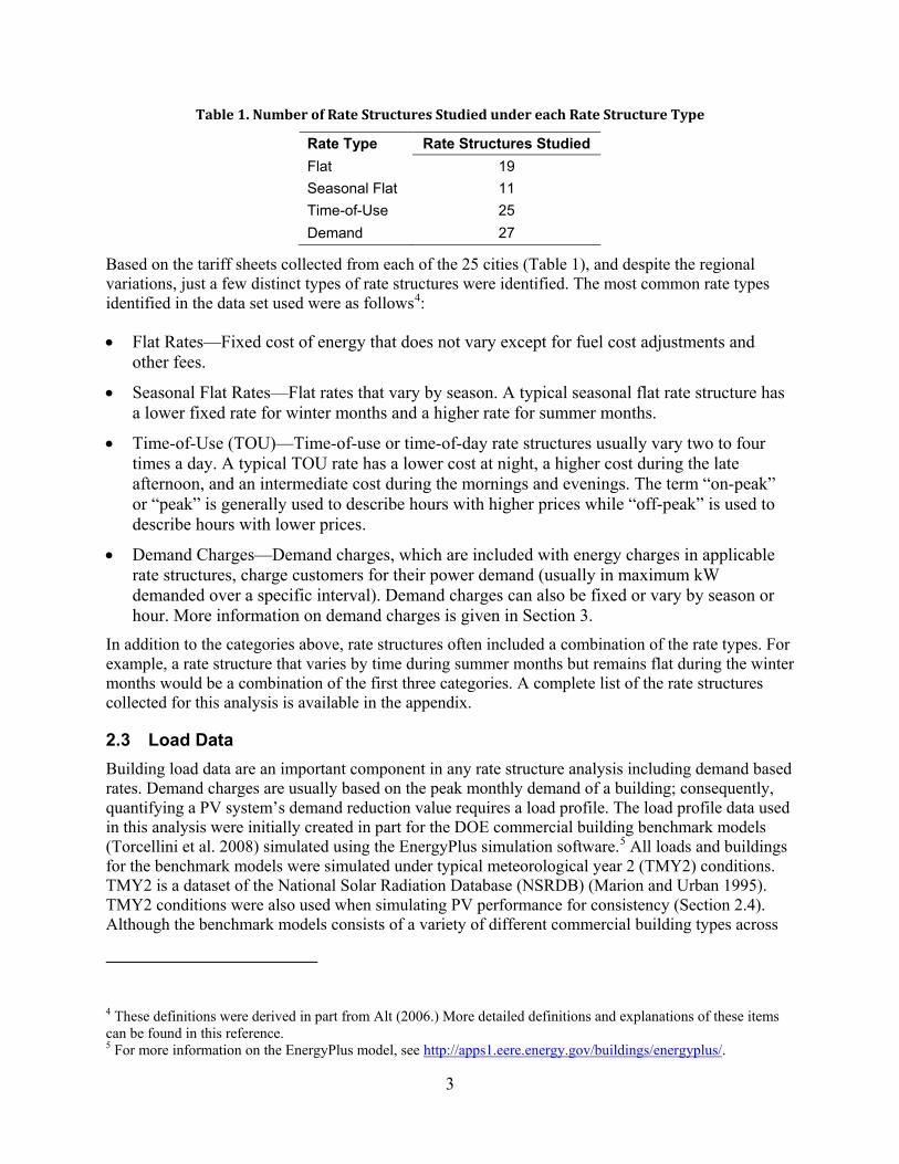
Table 1. Number of Rate Structures Studied under each Rate Structure Type

Rate Type Rate Structures Studied Flat 19 Seasonal Flat 11 Time-of-Use 25 Demand 27

Based on the tariff sheets collected from each of the 25 cities (Table 1), and despite the regional variations, just a few distinct types of rate structures were identified. The most common rate types identified in the data set used were as follows4

• Flat Rates—Fixed cost of energy that does not vary except for fuel cost adjustments and other fees.

:

• Seasonal Flat Rates—Flat rates that vary by season. A typical seasonal flat rate structure has a lower fixed rate for winter months and a higher rate for summer months.

• Time-of-Use (TOU)—Time-of-use or time-of-day rate structures usually vary two to four times a day. A typical TOU rate has a lower cost at night, a higher cost during the late afternoon, and an intermediate cost during the mornings and evenings. The term “on-peak” or “peak” is generally used to describe hours with higher prices while “off-peak” is used to describe hours with lower prices.

• Demand Charges—Demand charges, which are included with energy charges in applicable rate structures, charge customers for their power demand (usually in maximum kW demanded over a specific interval). Demand charges can also be fixed or vary by season or hour. More information on demand charges is given in Section 3.

In addition to the categories above, rate structures often included a combination of the rate types. For example, a rate structure that varies by time during summer months but remains flat during the winter months would be a combination of the first three categories. A complete list of the rate structures collected for this analysis is available in the appendix.

2.3 Load Data Building load data are an important component in any rate structure analysis including demand based rates. Demand charges are usually based on the peak monthly demand of a building; consequently, quantifying a PV system’s demand reduction value requires a load profile. The load profile data used in this analysis were initially created in part for the DOE commercial building benchmark models (Torcellini et al. 2008) simulated using the EnergyPlus simulation software.5

4 These definitions were derived in part from Alt (2006.) More detailed definitions and explanations of these items can be found in this reference.

All loads and buildings for the benchmark models were simulated under typical meteorological year 2 (TMY2) conditions. TMY2 is a dataset of the National Solar Radiation Database (NSRDB) (Marion and Urban 1995). TMY2 conditions were also used when simulating PV performance for consistency (Section 2.4). Although the benchmark models consists of a variety of different commercial building types across

5 For more information on the EnergyPlus model, see http://apps1.eere.energy.gov/buildings/energyplus/.

4

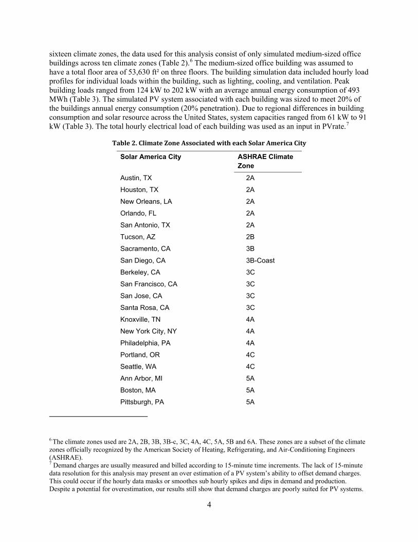
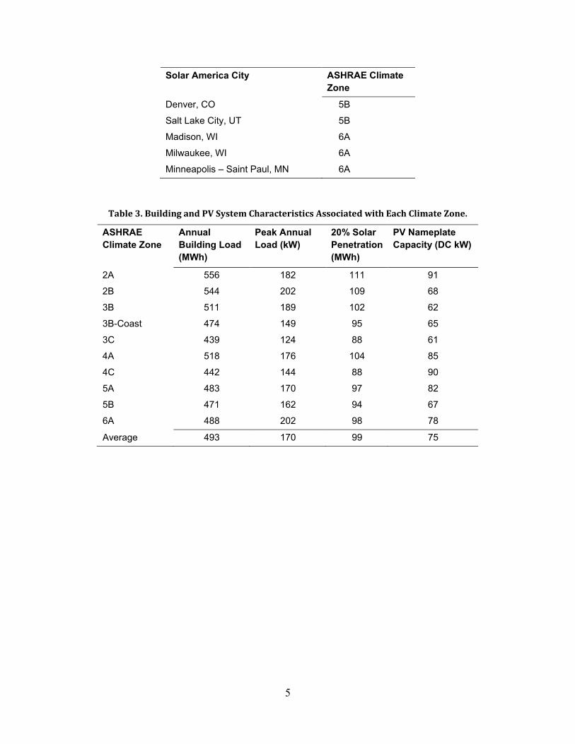
sixteen climate zones, the data used for this analysis consist of only simulated medium-sized office buildings across ten climate zones (Table 2).6 The medium-sized office building was assumed to have a total floor area of 53,630 ft² on three floors. The building simulation data included hourly load profiles for individual loads within the building, such as lighting, cooling, and ventilation. Peak building loads ranged from 124 kW to 202 kW with an average annual energy consumption of 493 MWh (Table 3). The simulated PV system associated with each building was sized to meet 20% of the buildings annual energy consumption (20% penetration). Due to regional differences in building consumption and solar resource across the United States, system capacities ranged from 61 kW to 91 kW (Table 3). The total hourly electrical load of each building was used as an input in PVrate.7

Table 2. Climate Zone Associated with each Solar America City

Solar America City ASHRAE Climate Zone

Austin, TX 2A

Houston, TX 2A

New Orleans, LA 2A

Orlando, FL 2A

San Antonio, TX 2A

Tucson, AZ 2B

Sacramento, CA 3B

San Diego, CA 3B-Coast

Berkeley, CA 3C

San Francisco, CA 3C

San Jose, CA 3C

Santa Rosa, CA 3C

Knoxville, TN 4A

New York City, NY 4A

Philadelphia, PA 4A

Portland, OR 4C

Seattle, WA 4C

Ann Arbor, MI 5A

Boston, MA 5A

Pittsburgh, PA 5A

6 The climate zones used are 2A, 2B, 3B, 3B-c, 3C, 4A, 4C, 5A, 5B and 6A. These zones are a subset of the climate zones officially recognized by the American Society of Heating, Refrigerating, and Air-Conditioning Engineers (ASHRAE). 7 Demand charges are usually measured and billed according to 15-minute time increments. The lack of 15-minute data resolution for this analysis may present an over estimation of a PV system’s ability to offset demand charges. This could occur if the hourly data masks or smoothes sub hourly spikes and dips in demand and production. Despite a potential for overestimation, our results still show that demand charges are poorly suited for PV systems.

5

Solar America City ASHRAE Climate Zone

Denver, CO 5B

Salt Lake City, UT 5B

Madison, WI 6A

Milwaukee, WI 6A

Minneapolis – Saint Paul, MN 6A

Table 3. Building and PV System Characteristics Associated with Each Climate Zone.

ASHRAE Climate Zone

Annual Building Load (MWh)

Peak Annual Load (kW)

20% Solar Penetration (MWh)

PV Nameplate Capacity (DC kW)

2A 556 182 111 91

2B 544 202 109 68

3B 511 189 102 62

3B-Coast 474 149 95 65

3C 439 124 88 61

4A 518 176 104 85

4C 442 144 88 90

5A 483 170 97 82

5B 471 162 94 67

6A 488 202 98 78

Average 493 170 99 75

6

2.4 Solar Data The PV production data used in this analysis were simulated using the typical meteorological year 28 (TMY2) dataset of the National Solar Radiation Database (NSRDB) (Marion and Urban 1995). The hourly solar data from the TMY2 dataset were converted into hourly PV production data using the PVWATTS model (Marion et al. 2005). A 77% AC-DC derate factor9

2.5 PV Savings Metric

was used for a system facing south at a 25° tilt.

Accurately capturing the impacts of various rate structure elements on a PV system’s value can be difficult because electricity prices differ widely across the United States. The average retail price of electricity for the commercial sector in 2009 ranged from 6.5 cents/kWh (Idaho) to 18.0 cents/kWh (Connecticut).10 Price differences occur for a variety of reasons including but not limited to a region’s fuel mix, regulations, and transmission constraints.11

PV savings = (electric bill without PV – electric bill with PV)/(electric bill without PV)*100%.

This analysis focuses on the relative savings impact due to the utility rate structure, as opposed to the absolute savings (or value) of a PV system. The primary metric used in this analysis is the PV savings metric, defined as the fraction of the annual electricity cost saved by the PV system:

This metric allows us to abstract from rate levels, thereby isolating the effects of the rate structure as opposed to regional differences in energy prices. A further example of this metric is to consider two different flat rates—one at 5 cents/kWh and another at 10 cents/kWh. In both cases, the PV system analyzed would offset 20% of the annual energy and thus 20% of the annual electricity charges. Because the rate structures are exactly the same (flat), they have the same PV benefit of offsetting 20% of annual costs.

8 Although TMY3 data were available at the time of this analysis, the TMY2 data were used because the DOE Benchmark buildings simulation data were also simulated using the TMY2 data. This allows for a more consistent treatment of building demand reduction and demand charge benefits. 9 A 77% derate factor is used primarily for residential PV systems and is considered conservative for commercial PV applications. 10 http://www.eia.doe.gov/cneaf/electricity/epm/table5_6_b.html. Last accessed February 3, 2010. 11 For more information on regional electricity price variations, see http://tonto.eia.doe.gov/energyexplained/index.cfm?page=electricity_factors_affecting_prices. Last accessed February 10, 2010.

7

3 Results and Discussion

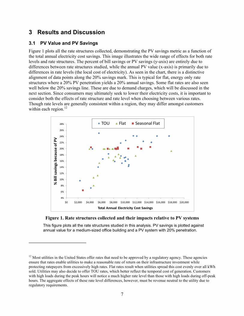
3.1 PV Value and PV Savings Figure 1 plots all the rate structures collected, demonstrating the PV savings metric as a function of the total annual electricity cost savings. This image illustrates the wide range of effects for both rate levels and rate structures. The percent of bill savings or PV savings (y-axis) are entirely due to differences between rate structures studied, while the annual PV value (x-axis) is primarily due to differences in rate levels (the local cost of electricity). As seen in the chart, there is a distinctive alignment of data points along the 20% savings mark. This is typical for flat, energy only rate structures where a 20% PV penetration yields a 20% annual savings. Some flat rates are also seen well below the 20% savings line. These are due to demand charges, which will be discussed in the next section. Since consumers may ultimately seek to lower their electricity costs, it is important to consider both the effects of rate structure and rate level when choosing between various rates. Though rate levels are generally consistent within a region, they may differ amongst customers within each region.12

Figure 1. Rate structures collected and their impacts relative to PV systems This figure plots all the rate structures studied in this analysis. PV savings is plotted against annual value for a medium-sized office building and a PV system with 20% penetration.

12 Most utilities in the United States offer rates that need to be approved by a regulatory agency. These agencies ensure that rates enable utilities to make a reasonable rate of return on their infrastructure investment while protecting ratepayers from excessively high rates. Flat rates result when utilities spread this cost evenly over all kWh sold. Utilities may also decide to offer TOU rates, which better reflect the temporal cost of generation. Customers with high loads during the peak hours will notice a much higher rate level than those with high loads during off-peak hours. The aggregate effects of these rate level differences, however, must be revenue neutral to the utility due to regulatory requirements.

4%

6%

8%

10%

12%

14%

16%

18%

20%

22%

24%

26%

28%

$0 $2,000 $4,000 $6,000 $8,000 $10,000 $12,000 $14,000 $16,000 $18,000 $20,000

% B

ill s

avin

gs b

ecau

se o

f PV

Total Annual Electricity Cost Savings

TOU Flat Seasonal Flat

8

3.2 Demand Charges and PV systems Demand charges are billed to customers based on how much power they demand during a particular interval. This interval is commonly 15 minutes; however, some utilities may use other timeframes. Utilities usually charge for peak monthly demands (Alt 2006), and these charges are usually billed in addition to energy charges. The following example illustrates the difference between energy and demand charges: a 100-Watt light bulb running for 10 hours uses the same amount of energy as a 1000-Watt heater running for 1 hour (1 kWh of energy). Although the customer will be charged equal amounts for the energy consumed by the bulb and the energy consumed by the heater, the heater will cost the customer more because it requires more power during a given period, driving up the demand charges.13

One of the more attractive features of solar technologies is their general correlation with peak demand (Denholm and Margolis 2007). In most parts of the United States, peak demand occurs during the afternoon of summer weekdays. Because of the high cost of peak power generation, common TOU electric rate structures charge users higher rates for use at peak times. As a result, PV becomes very attractive because it can provide a peak-shaving impact during the first few hours of the afternoon peak,

14

PV systems may offset a customer’s load by providing electricity during high demand hours. However, because demand is often measured in 15-minute intervals, if a PV system’s output is reduced as a result of clouds or maintenance during this peak load period, the actual benefit of PV on demand reduction can be substantially reduced. For buildings under a demand ratchet, this effect may be amplified.

offsetting expensive electricity from the grid.

15

13 This assumes the heater is used during the interval in which the peak demand is measured.

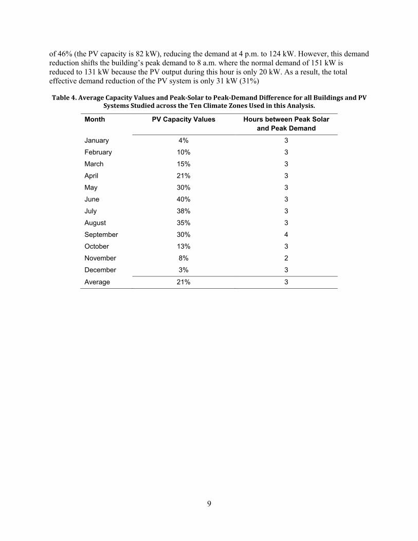
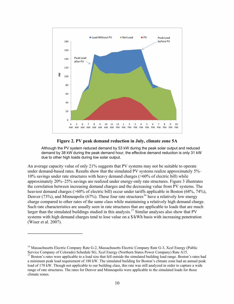
Additionally, peak building demand often occurs later in the afternoon, whereas PV output generally peaks at noon (standard time), depending on longitude. In these cases, PV systems cannot reduce peak loads by their full rated capacity, but rather a percentage of their capacity. Table 4 lists the capacity values of all PV systems studied. Here, the capacity value is defined as the total monthly peak demand reduction as a percentage of the PV systems’ rated capacity. The capacity value allows us to assess the actual impact on the monthly demand charge bill. Capacity values are highest during the summer months, averaging 38% between June and August compared to 6% between December and February. On average, peak PV production and peak demand occurs three hours apart for all months. On a clear day, PV systems can provide between 44% and 69% of rated capacity three hours from solar peak in December and June respectively. This sets a fundamental limit on the capacity value, which is dependent on the peak demand coincidence. Due in part to this limit as well as cloud cover and other hours of high demand, the capacity values approach a maximum of 40% during the summer and averages 21% for all months. Figure 2 illustrates several factors that affect PV capacity value. Here, the building’s normal peak load of 162 kW (without PV) occurs at 4 p.m. The PV output during this hour is equal to 38 kW, which is equal to a capacity value

14 The afternoon summer peak usually occurs between 1 p.m. and 7 p.m., while PV generation peaks between 10 a.m. and 3 p.m., depending on the longitude and latitude. The maximum system peak occurs around 3 p.m. to 4 p.m. local time (Denholm 2007) 15 Companies that operate under demand ratchets (usually larger loads) are billed for a percentage of their peak annual demand regardless of their actual monthly consumption. For example, a company that uses 1 MW during any hour in the previous 12 months is billed for 750 kW (if under a 75% ratchet) for all other months whether it uses any power the rest of the year. Such customers may have little incentive to install PV systems, given their variability in demand reduction.

9

of 46% (the PV capacity is 82 kW), reducing the demand at 4 p.m. to 124 kW. However, this demand reduction shifts the building’s peak demand to 8 a.m. where the normal demand of 151 kW is reduced to 131 kW because the PV output during this hour is only 20 kW. As a result, the total effective demand reduction of the PV system is only 31 kW (31%)

Table 4. Average Capacity Values and Peak-Solar to Peak-Demand Difference for all Buildings and PV Systems Studied across the Ten Climate Zones Used in this Analysis.

Month PV Capacity Values Hours between Peak Solar and Peak Demand

January 4% 3

February 10% 3

March 15% 3

April 21% 3

May 30% 3

June 40% 3

July 38% 3

August 35% 3

September 30% 4

October 13% 3

November 8% 2

December 3% 3

Average 21% 3

10

Figure 2. PV peak demand reduction in July, climate zone 5A Although the PV system reduced demand by 53 kW during the peak solar output and reduced demand by 38 kW during the peak demand hour, the effective demand reduction is only 31 kW due to other high loads during low solar output.

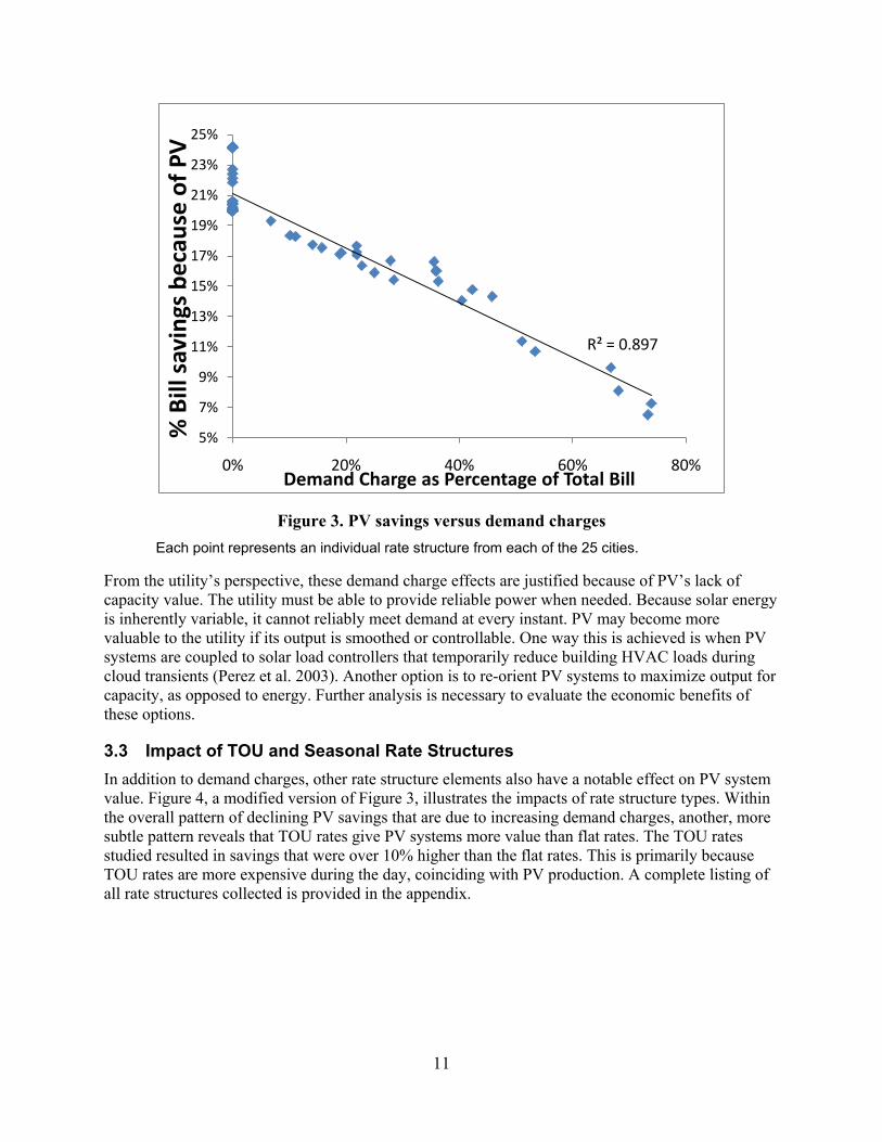
An average capacity value of only 21% suggests that PV systems may not be suitable to operate under demand-based rates. Results show that the simulated PV systems realize approximately 5%–10% savings under rate structures with heavy demand charges (>60% of electric bill) while approximately 20%–25% savings are realized under energy-only rate structures. Figure 3 illustrates the correlation between increasing demand charges and the decreasing value from PV systems. The heaviest demand charges (>60% of electric bill) occur under tariffs applicable in Boston (68%, 74%), Denver (73%), and Minneapolis (67%). These four rate structures16 have a relatively low energy charge compared to other rates of the same class while maintaining a relatively high demand charge. Such rate characteristics are usually seen in rate structures that are applicable to loads that are much larger than the simulated buildings studied in this analysis.17

16 Massachusetts Electric Company Rate G-2, Massachusetts Electric Company Rate G-3, Xcel Energy (Public Service Company of Colorado) Schedule SG, Xcel Energy (Northern States Power Company) Rate A15.

Similar analyses also show that PV systems with high demand charges tend to lose value on a $/kWh basis with increasing penetration (Wiser et al. 2007).

17 Boston’s rates were applicable to a load size that fell outside the simulated building load range. Boston’s rates had a minimum peak load requirement of 180 kW. The simulated building for Boston’s climate zone had an annual peak load of 170 kW. Though not applicable to our building class, this rate was still analyzed in order to capture a wide range of rate structures. The rates for Denver and Minneapolis were applicable to the simulated loads for those climate zones.

0

20

40

60

80

100

120

140

160

180

4 AM

5 AM

6 AM

7 AM

8 AM

9 AM

10 AM

11 AM

12 PM

1 PM

2 PM

3 PM

4 PM

5 PM

6 PM

7 PM

8 PM

9 PM

10 PM

KW

Load Without PV Net Load PV Peak Load before PV

Peak Load after PV

11

Figure 3. PV savings versus demand charges Each point represents an individual rate structure from each of the 25 cities.

From the utility’s perspective, these demand charge effects are justified because of PV’s lack of capacity value. The utility must be able to provide reliable power when needed. Because solar energy is inherently variable, it cannot reliably meet demand at every instant. PV may become more valuable to the utility if its output is smoothed or controllable. One way this is achieved is when PV systems are coupled to solar load controllers that temporarily reduce building HVAC loads during cloud transients (Perez et al. 2003). Another option is to re-orient PV systems to maximize output for capacity, as opposed to energy. Further analysis is necessary to evaluate the economic benefits of these options.

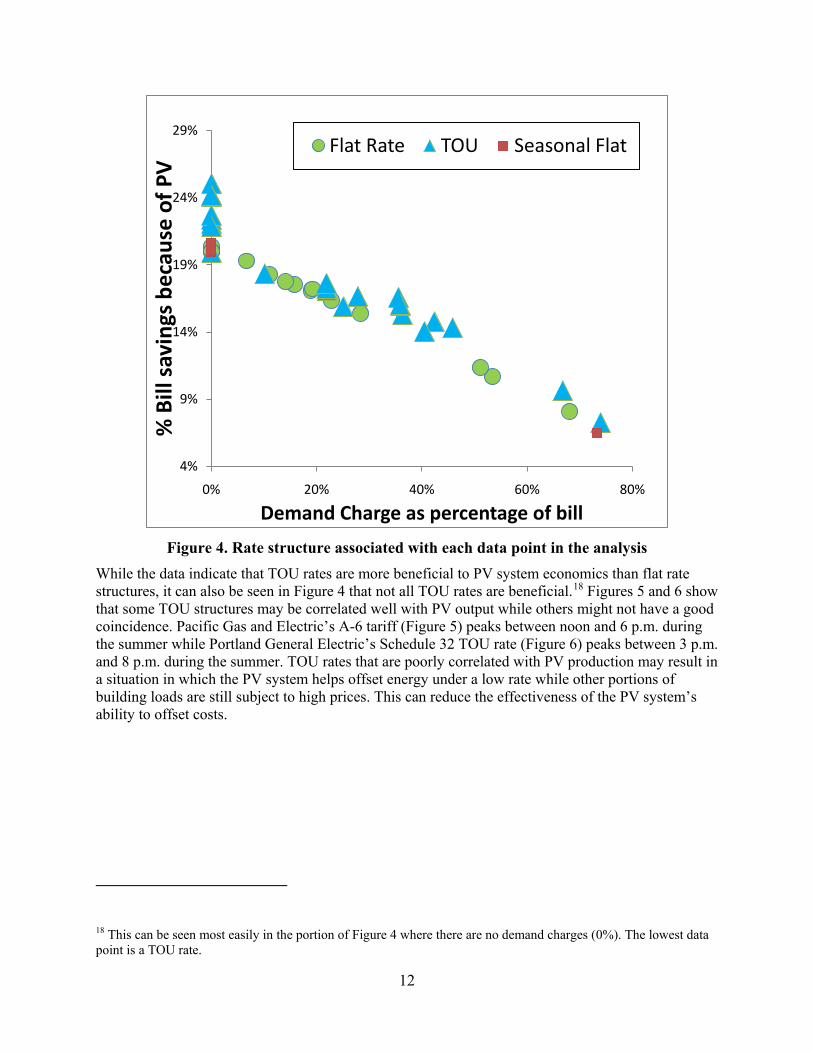
3.3 Impact of TOU and Seasonal Rate Structures In addition to demand charges, other rate structure elements also have a notable effect on PV system value. Figure 4, a modified version of Figure 3, illustrates the impacts of rate structure types. Within the overall pattern of declining PV savings that are due to increasing demand charges, another, more subtle pattern reveals that TOU rates give PV systems more value than flat rates. The TOU rates studied resulted in savings that were over 10% higher than the flat rates. This is primarily because TOU rates are more expensive during the day, coinciding with PV production. A complete listing of all rate structures collected is provided in the appendix.

R² = 0.897

5%

7%

9%

11%

13%

15%

17%

19%

21%

23%

25%

0% 20% 40% 60% 80%

% B

ill s

avin

gs b

ecau

se o

f PV

Demand Charge as Percentage of Total Bill

12

Figure 4. Rate structure associated with each data point in the analysis While the data indicate that TOU rates are more beneficial to PV system economics than flat rate structures, it can also be seen in Figure 4 that not all TOU rates are beneficial.18

18 This can be seen most easily in the portion of Figure 4 where there are no demand charges (0%). The lowest data point is a TOU rate.

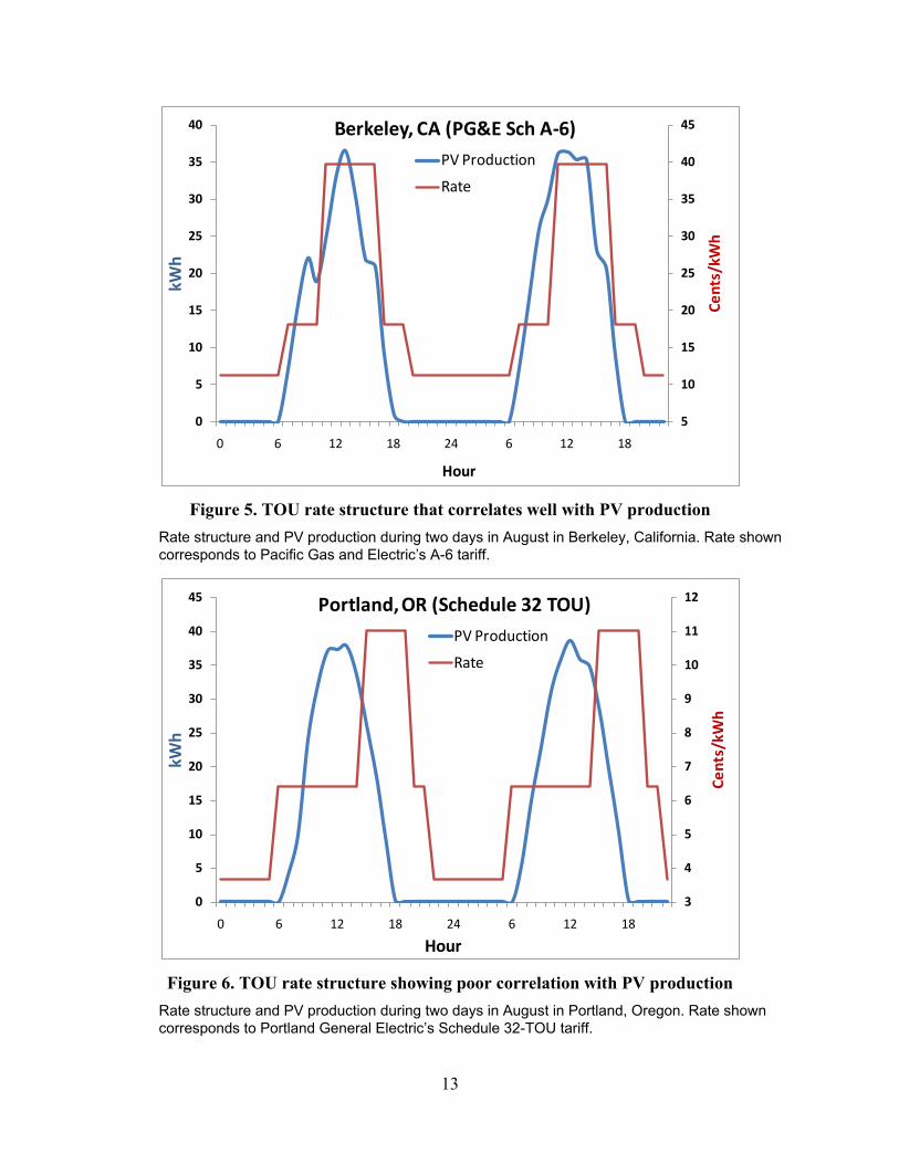
Figures 5 and 6 show that some TOU structures may be correlated well with PV output while others might not have a good coincidence. Pacific Gas and Electric’s A-6 tariff (Figure 5) peaks between noon and 6 p.m. during the summer while Portland General Electric’s Schedule 32 TOU rate (Figure 6) peaks between 3 p.m. and 8 p.m. during the summer. TOU rates that are poorly correlated with PV production may result in a situation in which the PV system helps offset energy under a low rate while other portions of building loads are still subject to high prices. This can reduce the effectiveness of the PV system’s ability to offset costs.

4%

9%

14%

19%

24%

29%

0% 20% 40% 60% 80%

% B

ill s

avin

gs b

ecau

se o

f PV

Demand Charge as percentage of bill

Flat Rate TOU Seasonal Flat

13

Figure 5. TOU rate structure that correlates well with PV production Rate structure and PV production during two days in August in Berkeley, California. Rate shown corresponds to Pacific Gas and Electric’s A-6 tariff.

Figure 6. TOU rate structure showing poor correlation with PV production Rate structure and PV production during two days in August in Portland, Oregon. Rate shown corresponds to Portland General Electric’s Schedule 32-TOU tariff.

5

10

15

20

25

30

35

40

45

0

5

10

15

20

25

30

35

40

0 6 12 18 24 6 12 18

Cent

s/kW

h

kWh

Hour

Berkeley, CA (PG&E Sch A-6)PV Production

Rate

3

4

5

6

7

8

9

10

11

12

0

5

10

15

20

25

30

35

40

45

0 6 12 18 24 6 12 18

Cent

s/kW

h

kWh

Hour

Portland, OR (Schedule 32 TOU)PV Production

Rate

14

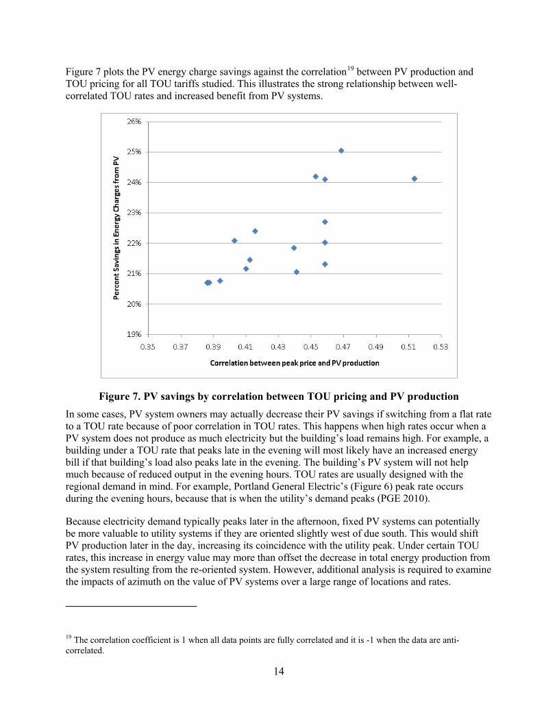
Figure 7 plots the PV energy charge savings against the correlation19

between PV production and TOU pricing for all TOU tariffs studied. This illustrates the strong relationship between well-correlated TOU rates and increased benefit from PV systems.

Figure 7. PV savings by correlation between TOU pricing and PV production In some cases, PV system owners may actually decrease their PV savings if switching from a flat rate to a TOU rate because of poor correlation in TOU rates. This happens when high rates occur when a PV system does not produce as much electricity but the building’s load remains high. For example, a building under a TOU rate that peaks late in the evening will most likely have an increased energy bill if that building’s load also peaks late in the evening. The building’s PV system will not help much because of reduced output in the evening hours. TOU rates are usually designed with the regional demand in mind. For example, Portland General Electric’s (Figure 6) peak rate occurs during the evening hours, because that is when the utility’s demand peaks (PGE 2010).

Because electricity demand typically peaks later in the afternoon, fixed PV systems can potentially be more valuable to utility systems if they are oriented slightly west of due south. This would shift PV production later in the day, increasing its coincidence with the utility peak. Under certain TOU rates, this increase in energy value may more than offset the decrease in total energy production from the system resulting from the re-oriented system. However, additional analysis is required to examine the impacts of azimuth on the value of PV systems over a large range of locations and rates.

19 The correlation coefficient is 1 when all data points are fully correlated and it is -1 when the data are anti-correlated.

15

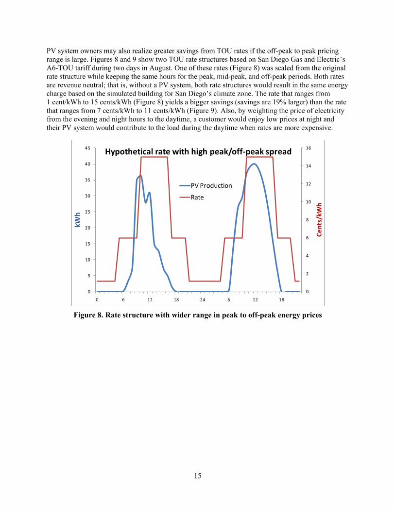
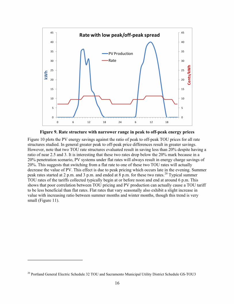
PV system owners may also realize greater savings from TOU rates if the off-peak to peak pricing range is large. Figures 8 and 9 show two TOU rate structures based on San Diego Gas and Electric’s A6-TOU tariff during two days in August. One of these rates (Figure 8) was scaled from the original rate structure while keeping the same hours for the peak, mid-peak, and off-peak periods. Both rates are revenue neutral; that is, without a PV system, both rate structures would result in the same energy charge based on the simulated building for San Diego’s climate zone. The rate that ranges from 1 cent/kWh to 15 cents/kWh (Figure 8) yields a bigger savings (savings are 19% larger) than the rate that ranges from 7 cents/kWh to 11 cents/kWh (Figure 9). Also, by weighting the price of electricity from the evening and night hours to the daytime, a customer would enjoy low prices at night and their PV system would contribute to the load during the daytime when rates are more expensive.

Figure 8. Rate structure with wider range in peak to off-peak energy prices

0

2

4

6

8

10

12

14

16

0

5

10

15

20

25

30

35

40

45

0 6 12 18 24 6 12 18

Cent

s/kW

h

kWh

Hypothetical rate with high peak/off-peak spread

PV Production

Rate

16

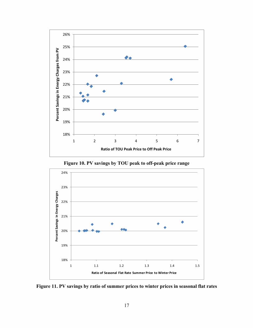
Figure 9. Rate structure with narrower range in peak to off-peak energy prices Figure 10 plots the PV energy savings against the ratio of peak to off-peak TOU prices for all rate structures studied. In general greater peak to off-peak price differences result in greater savings. However, note that two TOU rate structures evaluated result in saving less than 20% despite having a ratio of near 2.5 and 3. It is interesting that these two rates drop below the 20% mark because in a 20% penetration scenario, PV systems under flat rates will always result in energy charge savings of 20%. This suggests that switching from a flat rate to one of these two TOU rates will actually decrease the value of PV. This effect is due to peak pricing which occurs late in the evening. Summer peak rates started at 2 p.m. and 3 p.m. and ended at 8 p.m. for these two rates.20

20 Portland General Electric Schedule 32 TOU and Sacramento Municipal Utility District Schedule GS-TOU3

Typical summer TOU rates of the tariffs collected typically begin at or before noon and end at around 6 p.m. This shows that poor correlation between TOU pricing and PV production can actually cause a TOU tariff to be less beneficial than flat rates. Flat rates that vary seasonally also exhibit a slight increase in value with increasing ratio between summer months and winter months, though this trend is very small (Figure 11).

0

5

10

15

20

25

30

35

40

45

0

5

10

15

20

25

30

35

40

45

0 6 12 18 24 6 12 18

Cent

s/kW

h

kWh

Rate with low peak/off-peak spread

PV Production

Rate

17

Figure 10. PV savings by TOU peak to off-peak price range

Figure 11. PV savings by ratio of summer prices to winter prices in seasonal flat rates

18%

19%

20%

21%

22%

23%

24%

25%

26%

1 2 3 4 5 6 7

Perc

ent S

avin

gs in

Ene

rgy

Char

ges

from

PV

Ratio of TOU Peak Price to Off Peak Price

18%

19%

20%

21%

22%

23%

24%

1 1.1 1.2 1.3 1.4 1.5

Perc

ent S

avin

gs i

n En

ergy

Cha

rges

Ratio of Seasonal Flat Rate Summer Price to Winter Price

18

4 Conclusions This effort gathered and analyzed 55 unique rate structures from 25 cities across ten U.S. climate zones. By using a fixed PV penetration across all locations, we were able to identify the impacts of individual rate structure components on the value of PV generation. Common rate structure elements that appear to increase the value of PV include:

• TOU tariffs with peak pricing that is well correlated with PV production

• TOU tariffs that have a wide range between off-peak prices and peak prices

• Seasonal flat tariffs that have a relatively higher price in the summer than winter. Alternately, tariffs with demand charges tend to decrease the value of PV production. It was shown that PV systems, on average, have a relatively low capacity value, making them less attractive under rates with heavy demand charges. The results also indicate that although TOU rates are generally more beneficial to buildings with PV systems, some TOU rates are less beneficial than others are due to undesirable correlation between peak pricing and PV production.

Follow-up analyses could further clarify the relationship between additional rate structures, such as demand ratchets, block rates, and inverted block rates. Exploring how these findings would change in a scenario involving various PV penetration levels and various building types might yield significant insights into the impacts of rate structures. Finally, further studies could explore the concept that minor alterations in PV system design (such as facing the system slightly west) could maximize system economics under available rate structures.

19

References

Alt, L. E. (2006). “Energy Utility Rate Setting: A Practical Guide to the Retail Rate-Setting Process for Regulated Electric and Natural Gas Utilities.” Raleigh, NC: LuLu.

Borenstein, S. (2008). “The Market Value and Cost of Solar Photovoltaic Electricity Production.” CSEM WP 176. Berkeley, CA: Center for the Study of Energy Markets (CSEM). http://www.ucei.berkeley.edu/PDF/csemwp176.pdf

Denholm, P.; Margolis, R. (2007). “Evaluating the Limits of Solar Photovoltaics (PV) in Traditional Electric Power Systems.” Energy Policy (35:5); pp. 2853-2861.

Denholm, P.; R.M. Margolis; S. Ong; B. Roberts. (2009). “Break-Even Cost for Residential Photovoltaics in the United States: Key Drivers and Sensitivities.” NREL TP-6A2-46909. Golden, CO: National Renewable Energy Laboratory.

Doris E.; S. Ong, S.; Van Geet, O. (2009). “Rate Analysis of Two Photovoltaic Systems in San Diego.” NREL/TP-6A2-43537. Golden, CO: National Renewable Energy Laboratory.

Marion, B.; Anderberg. M.; Gray-Hann, P. (2005). “Recent Revisions to PVWATTS.” NREL/CP-520-38975. Golden, CO: National Renewable Energy Laboratory.

Marion, W.; Urban, K. (1995). “Users Manual for TMY2s Typical Meteorological Years.” Golden, CO: National Renewable Energy Laboratory.

Perez, R; Hoff, T; Herig, C; Shah J. (2003). “Maximizing PV Peak Shaving with Solar Load Control: Validation of a Web-based Economic Evaluation Tool.” Solar Energy (74); pp. 409-415.

PGE (Portland General Electric). (2010). Time of Use rate description Web page. http://www.portlandgeneral.com/residential/your_account/billing_payment/time_of_use/default.aspx. Accessed February 2010.

Solar Alliance. (2009). Utility Rates and Revenue Policies. http://www.solaralliance.org/four -pillars/utility-rates-revenue-policies.html. Accessed July 2, 2009.

Torcellini, P.; Deru, M.; Griffith, B.; Benne, K. ; Halverson, M.; Winiarski D. (2008). DOE “Commercial Building Benchmark Models.” NREL/CP-550-43291. Golden, CO: National Renewable Energy Laboratory.

Wiser, R.; Mills, A.; Barbose, G.; Golve, W. (2007). “The Impact of Retail Rate Structures on the Economics of Commercial Photovoltaic Systems in California.” LBNL-63019. Berkeley, CA: Ernest Orlando Lawrence Berkeley National Laboratory.

20

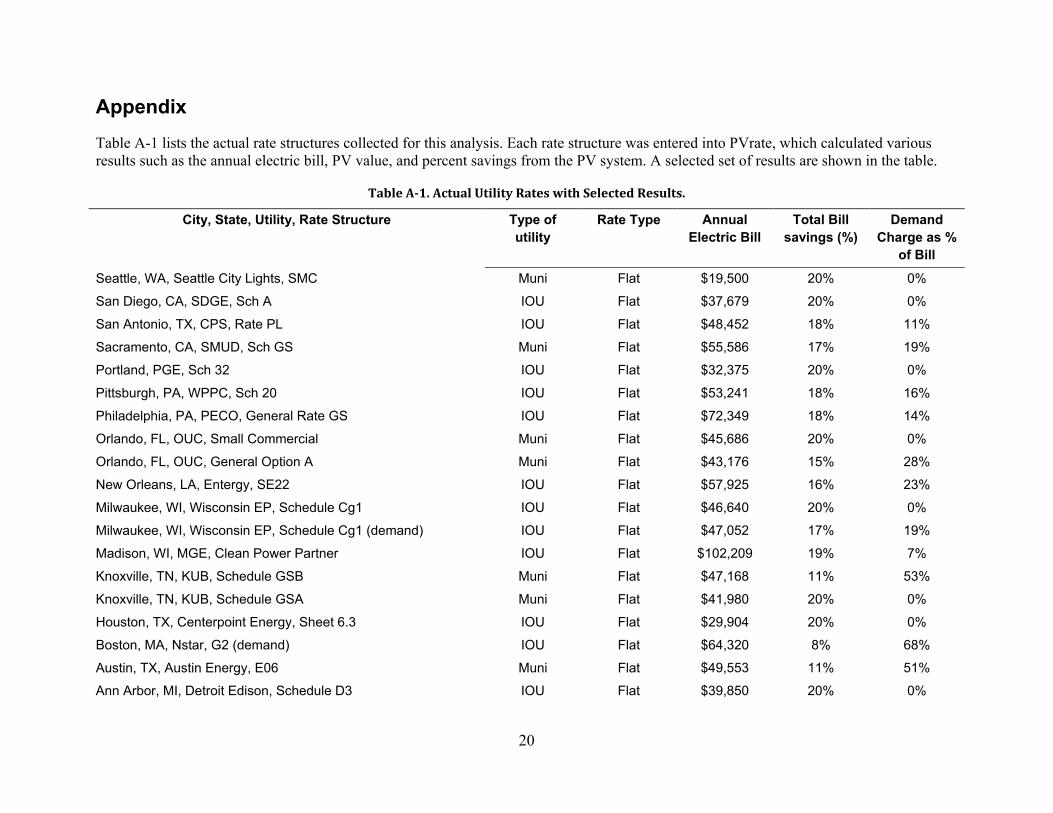
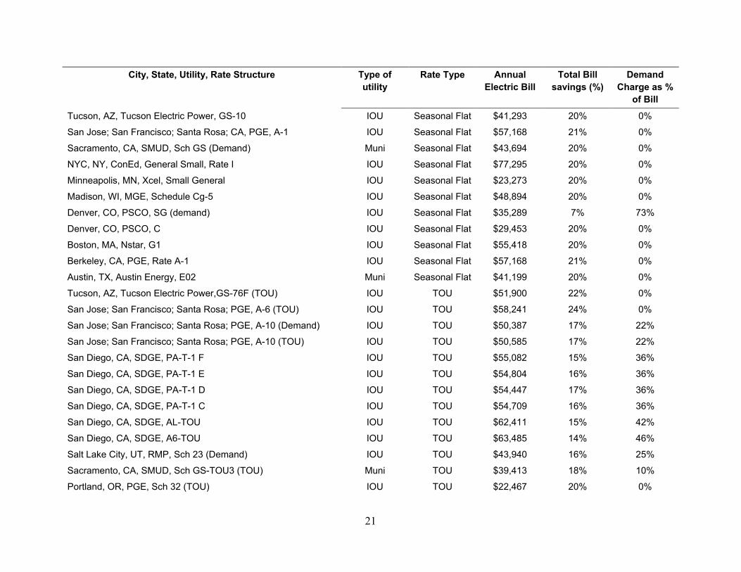
Appendix Table A-1 lists the actual rate structures collected for this analysis. Each rate structure was entered into PVrate, which calculated various results such as the annual electric bill, PV value, and percent savings from the PV system. A selected set of results are shown in the table.

Table A-1. Actual Utility Rates with Selected Results.

City, State, Utility, Rate Structure Type of utility

Rate Type Annual Electric Bill

Total Bill savings (%)

Demand Charge as %

of Bill

Seattle, WA, Seattle City Lights, SMC Muni Flat $19,500 20% 0%

San Diego, CA, SDGE, Sch A IOU Flat $37,679 20% 0%

San Antonio, TX, CPS, Rate PL IOU Flat $48,452 18% 11%

Sacramento, CA, SMUD, Sch GS Muni Flat $55,586 17% 19%

Portland, PGE, Sch 32 IOU Flat $32,375 20% 0%

Pittsburgh, PA, WPPC, Sch 20 IOU Flat $53,241 18% 16%

Philadelphia, PA, PECO, General Rate GS IOU Flat $72,349 18% 14%

Orlando, FL, OUC, Small Commercial Muni Flat $45,686 20% 0%

Orlando, FL, OUC, General Option A Muni Flat $43,176 15% 28%

New Orleans, LA, Entergy, SE22 IOU Flat $57,925 16% 23%

Milwaukee, WI, Wisconsin EP, Schedule Cg1 IOU Flat $46,640 20% 0%

Milwaukee, WI, Wisconsin EP, Schedule Cg1 (demand) IOU Flat $47,052 17% 19%

Madison, WI, MGE, Clean Power Partner IOU Flat $102,209 19% 7%

Knoxville, TN, KUB, Schedule GSB Muni Flat $47,168 11% 53%

Knoxville, TN, KUB, Schedule GSA Muni Flat $41,980 20% 0%

Houston, TX, Centerpoint Energy, Sheet 6.3 IOU Flat $29,904 20% 0%

Boston, MA, Nstar, G2 (demand) IOU Flat $64,320 8% 68%

Austin, TX, Austin Energy, E06 Muni Flat $49,553 11% 51%

Ann Arbor, MI, Detroit Edison, Schedule D3 IOU Flat $39,850 20% 0%

21

City, State, Utility, Rate Structure Type of utility

Rate Type Annual Electric Bill

Total Bill savings (%)

Demand Charge as %

of Bill

Tucson, AZ, Tucson Electric Power, GS-10 IOU Seasonal Flat $41,293 20% 0%

San Jose; San Francisco; Santa Rosa; CA, PGE, A-1 IOU Seasonal Flat $57,168 21% 0%

Sacramento, CA, SMUD, Sch GS (Demand) Muni Seasonal Flat $43,694 20% 0%

NYC, NY, ConEd, General Small, Rate I IOU Seasonal Flat $77,295 20% 0%

Minneapolis, MN, Xcel, Small General IOU Seasonal Flat $23,273 20% 0%

Madison, WI, MGE, Schedule Cg-5 IOU Seasonal Flat $48,894 20% 0%

Denver, CO, PSCO, SG (demand) IOU Seasonal Flat $35,289 7% 73%

Denver, CO, PSCO, C IOU Seasonal Flat $29,453 20% 0%

Boston, MA, Nstar, G1 IOU Seasonal Flat $55,418 20% 0%

Berkeley, CA, PGE, Rate A-1 IOU Seasonal Flat $57,168 21% 0%

Austin, TX, Austin Energy, E02 Muni Seasonal Flat $41,199 20% 0%

Tucson, AZ, Tucson Electric Power,GS-76F (TOU) IOU TOU $51,900 22% 0%

San Jose; San Francisco; Santa Rosa; PGE, A-6 (TOU) IOU TOU $58,241 24% 0%

San Jose; San Francisco; Santa Rosa; PGE, A-10 (Demand) IOU TOU $50,387 17% 22%

San Jose; San Francisco; Santa Rosa; PGE, A-10 (TOU) IOU TOU $50,585 17% 22%

San Diego, CA, SDGE, PA-T-1 F IOU TOU $55,082 15% 36%

San Diego, CA, SDGE, PA-T-1 E IOU TOU $54,804 16% 36%

San Diego, CA, SDGE, PA-T-1 D IOU TOU $54,447 17% 36%

San Diego, CA, SDGE, PA-T-1 C IOU TOU $54,709 16% 36%

San Diego, CA, SDGE, AL-TOU IOU TOU $62,411 15% 42%

San Diego, CA, SDGE, A6-TOU IOU TOU $63,485 14% 46%

Salt Lake City, UT, RMP, Sch 23 (Demand) IOU TOU $43,940 16% 25%

Sacramento, CA, SMUD, Sch GS-TOU3 (TOU) Muni TOU $39,413 18% 10%

Portland, OR, PGE, Sch 32 (TOU) IOU TOU $22,467 20% 0%

22

City, State, Utility, Rate Structure Type of utility

Rate Type Annual Electric Bill

Total Bill savings (%)

Demand Charge as %

of Bill

Orlando, FL, OUC, General Option B (TOU) IOU TOU $44,067 17% 28%

NYC, NY, ConEd, General Small, Rate II (TOU) IOU TOU $74,835 22% 0%

Minneapolis, MN, Xcel, Small General (TOU) IOU TOU $23,342 25% 0%

Minneapolis, MN, Xcel, General (TOU) IOU TOU $26,124 10% 67%

Milwaukee, WI, Wisconsin EP, Schedule Cg6 (TOU -B) IOU TOU $47,836 23% 0%

Milwaukee, WI, Wisconsin EP, Schedule Cg6 (TOU-A) IOU TOU $52,864 24% 0%

Milwaukee, WI, Wisconsin EP, Schedule Cg3 (TOU) IOU TOU $44,661 14% 40%

Madison, WI, MGE, Schedule Cg-3 (TOU) Muni TOU $50,777 24% 0%

Boston, MA, Nstar, G3 (TOU) IOU TOU $51,036 7% 74%

Berkeley, CA, PGE, Rate A-6 (TOU) IOU TOU $58,241 24% 0%

Berkeley, CA, PGE, Rate A-10 IOU TOU $50,596 18% 22%

Ann Arbor, MI, Detroit Edison, Schedule D3.4 IOU TOU $45,032 22% 0%

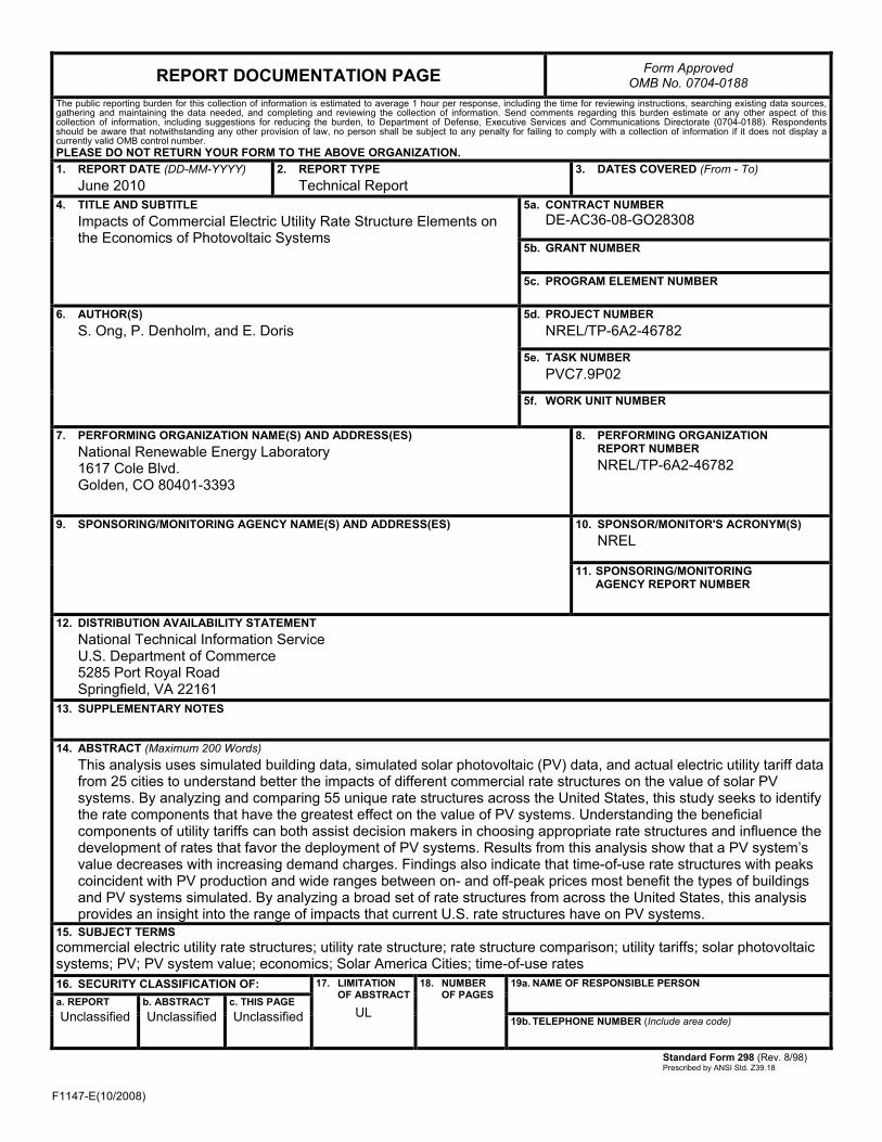
F1147-E(10/2008)

REPORT DOCUMENTATION PAGE Form Approved OMB No. 0704-0188

The public reporting burden for this collection of information is estimated to average 1 hour per response, including the time for reviewing instructions, searching existing data sources, gathering and maintaining the data needed, and completing and reviewing the collection of information. Send comments regarding this burden estimate or any other aspect of this collection of information, including suggestions for reducing the burden, to Department of Defense, Executive Services and Communications Directorate (0704-0188). Respondents should be aware that notwithstanding any other provision of law, no person shall be subject to any penalty for failing to comply with a collection of information if it does not display a currently valid OMB control number. PLEASE DO NOT RETURN YOUR FORM TO THE ABOVE ORGANIZATION. 1. REPORT DATE (DD-MM-YYYY)

June 2010 2. REPORT TYPE

Technical Report 3. DATES COVERED (From - To)

4. TITLE AND SUBTITLE

Impacts of Commercial Electric Utility Rate Structure Elements on the Economics of Photovoltaic Systems

5a. CONTRACT NUMBER DE-AC36-08-GO28308

5b. GRANT NUMBER

5c. PROGRAM ELEMENT NUMBER

6. AUTHOR(S) S. Ong, P. Denholm, and E. Doris

5d. PROJECT NUMBER NREL/TP-6A2-46782

5e. TASK NUMBER PVC7.9P02

5f. WORK UNIT NUMBER

7. PERFORMING ORGANIZATION NAME(S) AND ADDRESS(ES) National Renewable Energy Laboratory 1617 Cole Blvd. Golden, CO 80401-3393

8. PERFORMING ORGANIZATION REPORT NUMBER NREL/TP-6A2-46782

9. SPONSORING/MONITORING AGENCY NAME(S) AND ADDRESS(ES)

10. SPONSOR/MONITOR'S ACRONYM(S) NREL

11. SPONSORING/MONITORING AGENCY REPORT NUMBER

12. DISTRIBUTION AVAILABILITY STATEMENT National Technical Information Service U.S. Department of Commerce 5285 Port Royal Road Springfield, VA 22161

13. SUPPLEMENTARY NOTES

14. ABSTRACT (Maximum 200 Words) This analysis uses simulated building data, simulated solar photovoltaic (PV) data, and actual electric utility tariff data from 25 cities to understand better the impacts of different commercial rate structures on the value of solar PV systems. By analyzing and comparing 55 unique rate structures across the United States, this study seeks to identify the rate components that have the greatest effect on the value of PV systems. Understanding the beneficial components of utility tariffs can both assist decision makers in choosing appropriate rate structures and influence the development of rates that favor the deployment of PV systems. Results from this analysis show that a PV system’s value decreases with increasing demand charges. Findings also indicate that time-of-use rate structures with peaks coincident with PV production and wide ranges between on- and off-peak prices most benefit the types of buildings and PV systems simulated. By analyzing a broad set of rate structures from across the United States, this analysis provides an insight into the range of impacts that current U.S. rate structures have on PV systems.

15. SUBJECT TERMS commercial electric utility rate structures; utility rate structure; rate structure comparison; utility tariffs; solar photovoltaic systems; PV; PV system value; economics; Solar America Cities; time-of-use rates 16. SECURITY CLASSIFICATION OF: 17. LIMITATION

OF ABSTRACT

UL

18. NUMBER OF PAGES

19a. NAME OF RESPONSIBLE PERSON a. REPORT

Unclassified b. ABSTRACT Unclassified

c. THIS PAGE Unclassified 19b. TELEPHONE NUMBER (Include area code)

Standard Form 298 (Rev. 8/98) Prescribed by ANSI Std. Z39.18