imes discussion paper series - bank of japan · the postwar japanese economy keisuke otsu...
TRANSCRIPT
IMES DISCUSSION PAPER SERIES
INSTITUTE FOR MONETARY AND ECONOMIC STUDIES
BANK OF JAPAN
C.P.O BOX 203 TOKYO
100-8630 JAPAN
You can download this and other papers at the IMES Web site:
http://www.imes.boj.or.jp
Do not reprint or reproduce without permission.
A Neoclassical Analysis of the Postwar Japanese Economy
Keisuke Otsu
Discussion Paper No. 2007-E-1
NOTE: IMES Discussion Paper Series is circulated in
order to stimulate discussion and comments. Views
expressed in Discussion Paper Series are those of
authors and do not necessarily reflect those of
the Bank of Japan or the Institute for Monetary
and Economic Studies.
IMES Discussion Paper Series 2007-E-1 January 2007
A Neoclassical Analysis of
the Postwar Japanese Economy
Keisuke Otsu*
Abstract Two key features of the postwar Japanese economy are the delay of catch up during the 50s followed by rapid economic growth during the 60s and early 70s and the consistent decline in labor supply during the rapid growth period. A standard neoclassical growth model can quantitatively account for the Japanese postwar growth patterns of capital, output, consumption and investment taking the destruction of capital stock during the war and postwar TFP growth as given. The decline in labor can be explained by strong income effects caused by subsistence consumption during the rapidly growing period.
Keywords: Japanese Postwar Growth; Neoclassical Growth Model; TFP JEL classification: E13, O40
*Economist, Institute for Monetary and Economic Studies, Bank of Japan (E-mail: [email protected]) This paper is based on a chapter of my dissertation at UCLA. I thank my advisor Lee Ohanian for his advice and encouragement. I also like to thank Toni Braun and participants of workshops at IMES, the Bank of Japan and Osaka University for helpful discussions. Views expressed in this paper are those of the author and do not necessarily reflect the official views of the Bank of Japan.
1 Introduction
Two key features of the postwar Japanese economy are the delay of catch up dur-ing the 50s followed by rapid economic growth during the 60s and early 70s andthe consistent decline in labor supply during the rapid growth period. This paperquantitatively accounts for these features with a standard neoclassical growth model.The main objective of this paper is to quantitatively account for the impact of key
shocks on the postwar Japanese economy and understanding the channels throughwhich they operated within a standard neoclassical stochastic dynamic general equi-librium model. The model consists of an in�nitely lived representative household, a�rm with constant returns to scale production technology using capital and labor asinputs and a government who collects labor income tax and fully rebates with lump-sum transfer. I introduce the destruction of capital stock, TFP and labor wedges asexogenous shocks to the economy, compute the equilibrium, and compare the timepaths of key variables generated by the model to data from 1952 to 2000. The main�ndings are that the destruction capital stock and observed TFP can account for thegrowth pattern of postwar Japanese capital stock, output, consumption and invest-ment and that the decline in labor can be explained by strong income e¤ects causedby subsistence consumption during the rapidly growing period.Japanese postwar recovery has been a large topic in economic growth and de-
velopment literature. The interesting fact is that capital and output growth wasrapid during the 50s but dramatically accelerated during the 60s and 70s. Chris-tiano (1989) and King and Rebelo (1993) show that the destruction of capital stockalone within a neoclassical framework implies an unrealistically high return on cap-ital which causes counterfactually rapid capital accumulation immediately after thewar. They claim that preference with subsistence consumption can explain the delayin capital accumulation by encouraging agents to substitute consumption for invest-ment during early periods of recovery. Recent studies such as Chen, Imrohorogluand Imrohoroglu (2006) and Braun, Ikeda and Joines (2006) show that the neoclas-sical model with exogenous TFP and the loss of capital stock can account for thepostwar Japanese savings rate de�ned as capital stock accumulation. I show thatwith endogenous labor supply, subsistence consumption is not enough and that TFPis needed to explain the delay in catch up.Another interesting issue of the postwar Japanese economy is the consistent
decline in labor during the 60s and early 70s. With standard preference, exoge-nous wedges in the labor market formulated by Chari, Kehoe and McGrattan (2004)are important in explaining the �uctuation of labor. Ohanian, Ra¤o and Rogerson(2006) argue that a large part of this wedge can be explained by labor income tax
1
in OECD countries through. Unfortunately data on labor income tax in Japan isnot available for early 60s. In Braun, Ikeda and Joines (2006), this wedge is createdby exogenous changes in the family scale which a¤ects the utility weights betweenconsumption and leisure. Alternatively, I introduce a variation of the preference withsubsistence consumption used by Christiano (1989) and King and Rebelo (1993) andshow that the model can quantitatively account for the decline in labor throughstrong income e¤ects on leisure during the rapidly growing period without relyingon labor wedges.This paper has two major distinctions from recent literature on the postwar
Japanese economy such as Chen, Imrohologlu and Imrohologlu (2006), Braun, Ikedaand Joines (2006) and Braun, Okada and Sudou (2006). First, this paper focuses ongrowth paths of macroeconomic variables such as capital stock, output, consump-tion, investment and labor as opposed to saving rates, capital output ratios or �lteredseries. Instead of taking ratios or �ltering the time paths, I assess the data and simu-lated time paths in terms of their deviation from the balanced growth path. By doingso, the transition of each variable toward the steady state becomes clear. Second,labor wedge is explicitly included into the model with endogenous labor supply. Ishow that the model with preference which depends on subsistence consumption canquantitatively account for the decline in labor without relying on labor wedges.The remaining of the paper is organized as follows. Section 2 discusses empirical
regularities of the Japanese economy. Section 3 and 4 describes the benchmark modeland the quantitative method. Section 5 presents the quantitative results. Section 6concludes the paper.
2 Japanese Economy
In this section, I discuss the main facts of the Japanese economy during 1952-2000.Figure 1 shows the evolution of �ve key variables; capital stock, output, consumption,investment and labor per adult during this period. All variables except for labor arelogged and detrended with a 2% linear trend normalizing the 1989 values as 0. Themain objective of this paper is to understand the features of the evolution of thesevariables and why they followed such paths.First I present the growth accounting results and discuss how the economy evolved
on the production side. Next I turn to the demand side and assess the evolution ofGNP shares. These show that heavy investment took place in the 60s rather thanright after the war. This coincides with the period of highest output and productivitygrowth. Finally, I discuss the evolution of TFP and the labor wedge which I assumeto be exogenous. The data sources are Hayashi and Prescott (2002) for 1956-2000
2
and Ohkawa and Rosovsky (1973) for earlier periods.
2.1 Growth Accounting
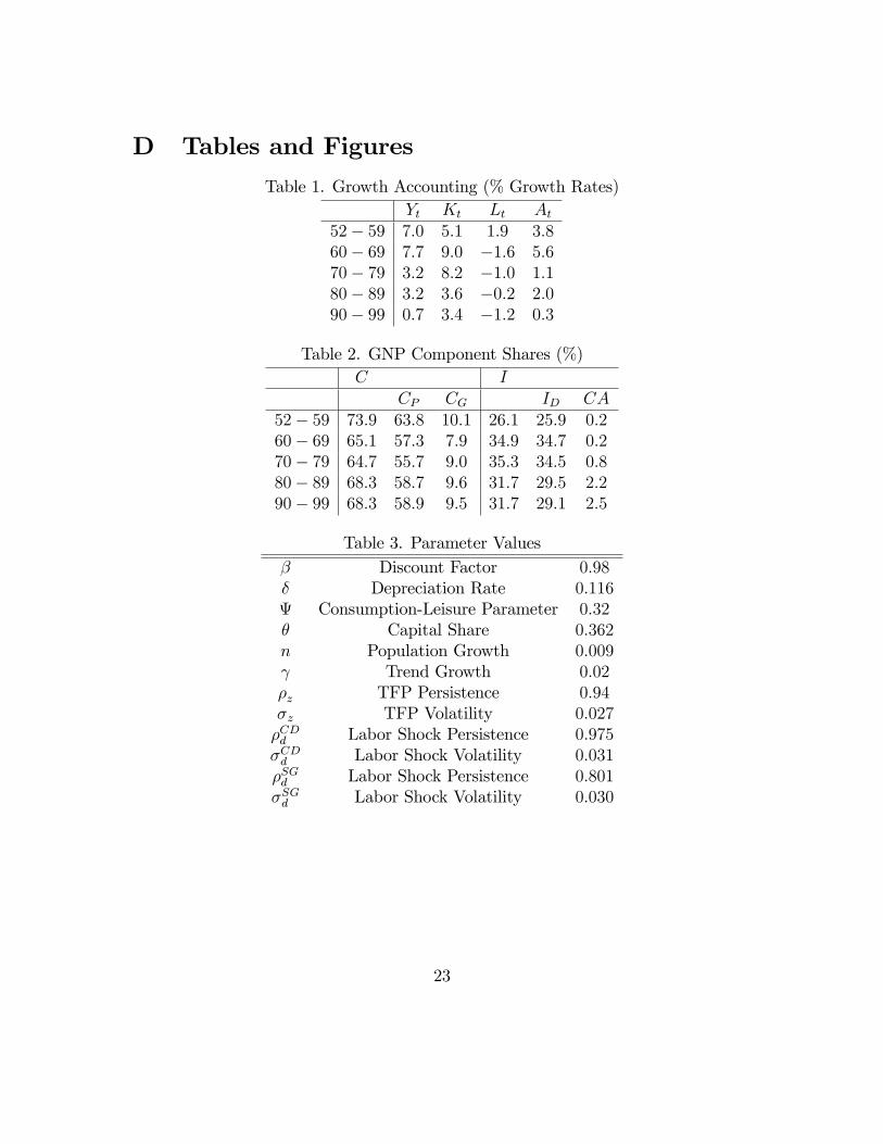
Table 1 shows the growth accounting results for Japan by decade. Growth accountingis based on the following Cobb-Douglas production function
Yt = AtK�t L
1��t : (1)
Output per adult Yt is GNP divided by working age population, i.e. the number ofpeople aged 20-69. Capital stock per adult Kt includes both private and governmentcapital stock1 held domestically, capital stock owned abroad and inventory stock.Labor input Lt is the number of people employed per adult times the average weeklyhours worked per worker. Capital share � is set at 0.362 which was computed byHayashi and Prescott (2002). Productivity At is computed as a residual in theproduction function which is also know as Solow residuals.The analysis starts from 1952 when the occupation by the allied powers ended. In
the 50s, the economy was growing at an average rate of 7.0%. A textbook explanationfor this fast growth in Japan would be that the destruction of capital stock during thewar created high marginal product of capital and led to rapid capital accumulation.However, output growth peaked in the 60s at 7:7%, not in the 50s. During the 50sthe growth rate of capital stock was only 2:8% and most of the growth came fromproductivity and labor growth. Capital stock started to grow rapidly during the 60s.After the 60s the economic growth slowed down but not monotonically. During the80s, the average growth rate was slightly above 3% and almost the same as in the70s while the growth rate fell below 1% during the 90s. The 80s is known as thebubble economy period where a common perception is that the economy was led byoverheated investment. However, growth accounting shows that TFP was actuallygrowing in a signi�cantly faster rate than in the 70s.An interesting feature of the postwar Japanese economy is the secular decline in
labor except for during the 50s. The decline in labor is especially outstanding duringthe 60s and early 70s where the 1975 level is 30% below the 1960 level. It turns outthat the main challenge of the theory is to explain this pattern on labor.
1Hayashi and Prescott (2002) abstract government owned capital stock from their analysis.However, since capital accumulation is one of the key issues in this paper, I add government capitalstock. The results in this paper are not sensitive to this di¤erence.
3
2.2 GNP Component Shares
Table 2 shows the evolution of GNP shares. The demand side of the economy isdivided into consumption and investment. The table shows that rapid investmenttook place in the 60s.Consumption consists of private consumption CP and government consumption
CG. For simplicity, I combine them together and treat them as total consumption2.Investment consists of gross domestic capital formation ID and current account CA.Gross domestic capital formation includes both private and government investmentas well as changes in inventories where inventory stocks are included in capital stock.Current account is included in investment where capital stock is adjusted for capitalstock owned abroad3. In short, the resource constraint is,
Yt = Ct + It = CPt + CGt + IDt + CAt: (2)
In the 50s, both private and government consumption share were in peak whiledomestic investment and current account were at the lowest. Domestic investmentgrew rapidly in 60s and peaked in 70s which indicates the rapid capital accumulationduring these periods. Current account improved dramatically in 80s and stayed highduring 90s. However, the share of current account on total GNP is not large and doesnot seem to be a major source of growth4. The share of both private and governmentconsumption fell in the 60s re�ecting the rapid increase in investment. Private con-sumption fell further in 70s and grew back in 80s. Government consumption grewback in 70s and stayed roughly constant.
2.3 Trend and Productivity Shocks
In order to incorporate the concept of balanced growth into the analysis, I alter theproduction technology from (1) to,
Yt = ztK�t (Xtlt)
1�� (3)
where zt is detrended TFP and Xt is the world technical progress. Obviously theSolow residual At in (1) is equal to ztX1��
t . World technical progress is assumed tofollow the process
Xt = (1 + )Xt�1 (4)
2Alternatively the model can include government consumption separately as an exogenous vari-able. This alternative speci�cation will not change the results of this paper.
3See Hayashi and Prescott (2002) for details.4There are studies such as Gilchrist and Williams (2004) which emphasize the importance of
trade in terms of importing technology embeded in vintage capital.
4
where is a constant growth rate which I assume to be 2%5. Along the balancedgrowth path, all variables except for labor should grow at this trend rate. In orderto make the system stationary, all growing variables are divided by Xt.Figure 2 shows the long run log output series linearly detrended by 2% setting
1905 as 0. This shows that Japan was in a steady state before the war and thatthe economy seems to have been growing towards a new steady state after war. Thesudden drop of output immediately after the war can be attributed to the loss ofcapital stock. However, a temporary loss of capital stock does not a¤ect the steadystate level of capital nor output. Thus, I conjecture that the steady state level ofz has increased, i.e. the balanced growth path shifted upwards. It is convenient toassume that there was a one-shot shift of the balance growth path after the war sincenow we can evaluate all variables as deviations from the new steady state. Parenteand Prescott (1994) suggest this shift is due to a reduction of barriers to technologyadoption after WWII6.Figure 3 shows linearly detrended postwar TFP and GNP setting the values in
1989 as the new steady state. Clearly, there is high positive correlation betweenTFP growth and GNP growth. The transition of TFP to its new steady state levelwas not instantaneous but gradual. Eaton and Kortum (1997) claims that a setof current leading economies including Japan experienced rapid growth and a slowdown in postwar productivity because of the gradual adoption of more productivetechnology. Gilchrist and Williams (2004) argues that the gradual growth of TFPcomes from the accumulation of vintage capital.In this paper, instead of modeling the source of TFP growth I take it as exoge-
nous. I implicitly assume that productivity grows because Japan gained access toleading technology after the war following Parente and Prescott (1994) and Eatonand Kortum (1997). Once technology reaches the balanced growth path, it will growat the same rate as the frontier7. Quantitative results show that TFP is importantin explaining the rapid capital accumulation during the60s and early 70s.
5This number is assumed to be the average trend growth rate in US in many studies such asKing and Rebelo (1993).
6They consider gradual reductions of barriers with multiple shifts in balance growth pathswhereas I assume that there is a one shot reduction in the barrier associated with a single shift inthe balanced growth path.
7There might be a gap between detrended steady state productivity in Japan and the frontierdue to a remaining barrier to the di¤usion of new ideas. Thus, convergence to the new steady stateis not necessarily equivalent to convergence to US productivity level.
5
2.4 Labor Wedge
In this section I introduce �labor wedges�which is known to be a powerful source oflabor �uctuation. Following Chari, Kehoe and McGrattan (2004), I compute laborwedge dt from the labor-leisure �rst order condition. That is,
�ultuctdt =MPlt:
Following the literature, labor wedge is modeled as distortionary labor income taxand is considered as an exogenous variable. In general, there are many other possiblesources of this wedge. Nonetheless labor wedges generated by other sources areobservationally equivalent to labor income tax in equilibrium. Since specifying thesource of labor wedge is beyond the scope of this paper, I do not further complicatethe model.Figure 4 plots the log deviation of labor and dt from their 1989 level where I
assume d1989 = 18. Labor wedges are computed for Cobb-Douglas preference andStone-Geary preference cases where the preference and the production functions aredescribed in the following section. Obviously labor wedges and labor are negativelycorrelated.Figure 4 also plots the log deviation of labor income tax series de�ned as 1
1��from their 1989 level. Ohanian, Ra¤o and Rogerson (2006) show that a large partof labor wedges in OECD countries can be explained by labor income taxes usingthe Mendoza, Razin and Tesar (1994) tax data. This data plotted by a dotted lineis based on the OECD revenue statistics which only goes back to 1965 for Japan.The solid line represents a crude measure of labor income tax computed as (laborshare) � (income tax)=(national income) using the Hayashi and Prescott (2002)dataset for labor share and Japanese Statistics Bureau data for the others in orderto complement the missing periods. The discrepancies between the labor incometax data and labor wedges imply that labor income tax is not the only source ofdistortion in the labor market.There are several other possible sources of labor wedges. Chari, Kehoe and
McGrattan (2004) shows that monetary shocks can generate �uctuation dt givensticky wages. In their model, money growth will a¤ect the price level which a¤ectsreal wages given sticky nominal wages. Thus, labor allocation will be distorted fromthe level of which the model would have generated without wage stickiness. Cooleyand Hansen (1989) show that money growth can create this disturbance through
8The selection of the steady state value d does not a¤ect the quantitative results much since itwill only a¤ect the calibration of the preference parameter .
6
a cash in advance constraint. In their model, �nal goods can be purchased onlywith cash where labor income earned after the purchase is divided into cash held fortomorrow and �nancial assets. Shocks to money growth a¤ect the relative price ofconsumption to labor through in�ation tax which is equal to the nominal interestrate. Christiano and Eichenbaum (1992) shows that the wedge can be caused byinterest rate shocks with a working capital on labor assumption. In this model,�rms must borrow resources in order to process wage payment so that shocks to theborrowing cost will a¤ect the e¤ective wages.There are also recent literatures which document possible sources of labor wedges
in Japan. Braun, Ikeda and Joines (2006) show that the decline in family sizes ina life-cycle model can account for the secular decrease in labor input through 1960-2000. In their model, family size determines the utility weights on consumptionrelative to leisure. Thus, the shift in family size works as labor wedges by a¤ecting themarginal rate of substitution of leisure for consumption. Inaba and Kobayashi (2005)claim that the continuously declining asset price can be a candidate for the labormarket deterioration during the 90s. In their model, there is a collateral constraintsuch that �nal goods can be purchased only up to a �xed amount of the currentvalue of land. A decline in asset prices which causes this constraint to bind increasesthe e¤ective price of �nal goods relative to labor.In this paper I show that the model with preference which depends on subsistence
consumption can quantitatively account for the decline in labor during the 60s andearly 70s without relying on labor wedges. The remaining role of labor wedges is toexplain the labor growth during the 50s and the labor drop during the 90s.
3 Model
In this section, I describe the model used to analyze the Japanese economy. Thefoundation of the model is a standard stochastic neoclassical growth model whichconsists of an in�nitely lived representative household who has preference over con-sumption and leisure and a �rm who uses constant returns to scale technology toconvert capital stock and labor into output. I also assume a government who collectslabor income tax and fully rebates by lump-sum transfer.
7
3.1 Household
The preference for the representative household depends on utility from consumptionand leisure;
maxU = E0
1Xt=0
�tu(ct; 1� lt) (5)
where � is the subjective discount rate such that 0 < � < 1, ct is detrended consump-tion and lt is labor supply which is the fraction of total hours available allocated towork9. For the functional form of u(�), I consider a Cobb-Douglas preference caseand a Stone-Geary preference case.The Cobb-Douglas preference function is widely used in macroeconomic litera-
ture;
u(ct; lt) =(ct (1� lt)1�)1��
1� � : (6)
� represents the relative risk aversion where 0 � � < 1 and is the weight thehousehold assigns to consumption where 0 < < 1.Stone-Geary preference function is used in growth literature such as Christiano
(1989) and King and Rebelo (1993);
u(ct; lt) =((ct � c)(1� lt)1�)1��
1� � : (7)
c � 0 is the subsistence level of consumption set at c = 0:35c such that initialconsumption is slightly higher than the subsistence level. This preference is consistentwith balanced growth since the subsistence consumption is de�ned as a constantrelative to the trend. (7) is slightly di¤erent from the preference used in Christiano(1989) and King and Rebelo (1993) since it includes leisure as an argument. It turnsout that this modi�cation brings several interesting implications on labor which isdiscussed in the following section.The household maximizes (5) subject to a budget constraint;
(1� � lt)wtlt + rtkt + Tt = ct + it: (8)
9In speci�c,
lt =EtNt
Ht16 � 7
where Et is the number of people employed, Nt is the adult population and Ht is the average weeklyhours worked per worker. I assume that the hours available to work per day are 16 hours.
8
� lt is labor income tax rate where1
1�� lt= dt and Tt is the lump-sum transfer. it is
detrended investment such that the capital law of motion;
(1 + )(1 + n)kt+1 = it + (1� �)kt (9)
holds. For simplicity, I assume that the population growth rate n is constant.
3.2 Firm
The detrended �rm�s problem is;
max�t = yt � wtlt � rtkt (10)
where yt, wt, rt are detrended output, wage and return on capital, and
yt = ztk�t l1��t : (11)
3.3 Government
For simplicity, I assume that the government rebates all the labor income tax col-lected by lump-sum transfer;
� ltwtlt ��1� 1
dt
�wtlt = Tt (12)
Notice that there are no sign restrictions on � lt such that when �lt < 0 the government
gives subsidy on working and a collects lump-sum tax. The role of government issimpli�ed as above since the key feature of interest is the labor market distortioncreated by labor income tax. Models such as Chari, Kehoe and McGrattan (2004)consider the role of government expenditure as an exogenous shock. It turns outthat the e¤ect of government purchase shocks is very small in Japan.
3.4 Shocks
The exogenous shocks are assumed to follow the process:�ln ztln dit
�=
��z 00 �id
��ln zt�1ln dit�1
�+
�"zt"idt
�;
�"zt"idt
�� N
�0;
��2z 00 (�id)
2
��: (13)
Where i = CD for Cobb-Douglas preference and i = SG for Stone-Geary preference.For simplicity, I assume that the shocks are uncorrelated. This simpli�cation does
9
not a¤ect the quantitative analysis since the linear decision rules do not depend onthe error terms and the simulation uses the observed shocks, not random draws fromthe joint distribution10.As mentioned in the previous section, I assume that there was a one-time upward
shift in the balance growth path after the war. The gap between initial TFP andthe new steady state shown in �gure 2 does not re�ect a drop in technological levelbut was caused by this rare event. Once the balanced growth path shifted out, theAR1 process gives the expected TFP growth rate as
ln zt � ln zt�1 = (�z � 1) ln zt�1:
This means that agents expect TFP growth to slow down as it approaches the steadystate.This is a very strong assumption for the shock process. This requires the agents
to know where the new steady state is from the beginning as well as the averageconvergence rate of technology to the new steady state level. Nonetheless, I use thissetting as a benchmark since it is a convenient way to simplify the model. Later Icompare di¤erent cases on expectation assumptions and show that the actual timepath of the shocks is important rather than the expectation generating process.
3.5 Equilibrium
A competitive equilibrium is, fct; lt; kt+1; yt; it; wt; rtg1t=0 such that;
1. Households optimize given fwt; rt; dtg1t=0 and k0
2. Firm optimizes given fwt; rt; ztg1t=03. Markets clear and the government budget constraint (12) holds.
4. The resource constraint holds:
yt = ct + it (14)
5. Shocks follow the exogenous process (13).
10The assumption on errors a¤ects the estimation of persistence parameters. With the simpli�-cation, OLS estimation can be used to obtain the parameter. However, if there were correlationsbetween shocks, OLS estimation on seemingly unrelated regression will lead to e¢ ciency loss inthe parameter estimation. It turns out that all of the quantitative results hold for wide ranges ofpersistence parameters.
10
The optimization yields the �rst order condition for labor;
�ultuctdt = (1� �)
ytlt
(15)
and the Euler equation for capital stock;
uct(1 + )(1 + n) = �Et
�uct+1
��yt+1kt+1
+ 1� ���
(16)
where the marginal utilities of consumption and labor are;
uct = c(1��)�1t (1� lt)(1�)(1��)
�ult = (1�)c(1��)t (1� lt)(1�)(1��)�1
for Cobb-Douglas preference and
uct = (ct � c)(1��)�1(1� lt)(1�)(1��)
�ult = (1�)(ct � c)(1��)(1� lt)(1�)(1��)�1
for Stone-Geary preference.
4 Quantitative Method
In this section, I describe how the quantitative analysis is conducted. First, I discusshow the parameter values were obtained from data. Most parameters were obtainedby calibration. Next, I describe the method used to simulate the time paths ofcapital stock, output, consumption, investment and labor. The simulation is basedon a standard dynamic stochastic general equilibrium solution method.
4.1 Parameter Values
Most of the parameter values were calibrated to data over the 1984-1989 period inJapan. The obtained parameter values are listed in table 3.� is calibrated by the steady state version of capital accumulation equation (9)
� = 1 +i
k� (1 + n)(1 + );
� was calibrated by the steady state version of the capital Euler equation (16);
(1 + )(1 + n) = �(�y
k+ 1� �);
11
and was calibrated by the steady state version of the labor �rst order condition(15);
1�
= (1� �)yc
1� ll
where n; ik; yk; and l were set at the data average, was set at 2% and � was borrowed
from Hayashi and Prescott (2002). �z and �d were estimated by a regression of theAR1 processes (13) for 1952-2000.
4.2 Simulation Method
The quantitative analysis uses linearized equilibrium conditions. I followed themethod introduced by Uhlig (1997) to compute linear decision rules for the endoge-nous variables. All variables are de�ned as their deviations from the steady statewhich I set at the 1989 value. Thus, the values of all variables in 1989 are 0. Thedeviation of a variable xt is de�ned as
ext = ln xt � lnx:The decision rules depend on state variables �capital stock and exogenous vari-
ables. I set capital stock at its actual level in the initial period 195211. I substitutelinearly detrended shocks into the linearized decision rules to compute the time pathsof the endogenous state variable �capital stock �for each period. Plugging the shocksand the simulated series of capital stock into the decision rules, I simulate the timepaths of other endogenous variables. Finally, I plot the simulation results of output,consumption, investment and labor and compare them to the linearly detrended datanormalizing the 1989 values as 0.Since the initial period is far away from the steady state, there is a fear that the
linearized model provides poor results for early periods. In the appendix I show thatresults from this linearized method is close to results from a nonlinear deterministicsimulation.11The detrended log deviation from steady state was �1:54 in the initial period. This implies that
the capital stock in 1952 was exp(�1:54) = 0:214 relative to the new steady state or in other words78:6% below the new steady state level. Existing literature such as Chen, Imrohologlu, Imrohologlu(2006) uses more moderate numbers since they capture the loss of capital stock relative to theprewar level which is considerably lower than the new steady state.
12
5 Results
In this section I conduct three types of simulations with both Cobb-Douglas andStone-Geary preferences. First, one with the destruction of capital as the only shockto the economy. Second, one with the destruction of capital and TFP shocks. Third,one with the destruction of capital and TFP and labor wedge shocks. For all cases,I set the relative risk aversion parameter � = 2 where all of the following resultshold with wide ranges of parameter values for � � 1. The results are presented in�gures 5, 6 and 7 where dotted lines and solid lines represent simulation results withCobb-Douglas and Stone-Geary preferences respectively.The results show that without TFP, the model cannot explain the features of
postwar Japanese economy. With Cobb-Douglas preference, the model with TFPcan explain the growth pattern of capital, output consumption and investment con-siderably well. However, in order to explain the drop of labor supply, the modelneeds labor wedges which exogenously increase during this period. On the otherhand, with Stone-Geary preference, the model with TFP can account for both therapid economic growth and labor decline during the 60s and early 70s without laborwedges. In the following, I summarize the results by each type of simulation carriedout.
5.1 Capital Loss
The �rst experiment uses capital destruction as the only shock to the economy12.This corresponds to the analysis of King and Rebelo (1993) which focuses on thetransitional dynamics of postwar economies. The results show that in both preferencecases the model cannot account for the delay of catch up.The reason why the model fails to explain the delay of catch up is because in the
earlier periods the marginal product of capital is too high due to the loss of capitalstock during the war. This causes the model to predict rapid capital accumulationimmediately after the war. Capital accumulation depends on � since this parametergoverns the intertemporal elasticity of substitution which represents the willingnessto smooth consumption over time by saving capital stock as discussed in King andRebelo (1993). However there is no realistic value of � that can quantitatively accountfor the time path of capital stock in both preference cases.Christiano (1989) and King and Rebelo (1993) claim that Stone-Geary prefer-
12In my model, low capital stock relative to the new steady state in the initial period is a resultof both the loss of capital stock during the war and the jump of steady state to a higher level. Forsimplicity, I will call this combined e¤ect as the destruction of capital.
13
ence can cause a delay in capital accumulation whereas my results show that bothpreferences give virtually the same outcome in terms of capital accumulation. Thereason my model cannot account for the delay of capital accumulation is because I in-clude leisure in the preference, or in other words because labor supply is endogenous.Since subsistence consumption increases the relative importance of consumption inearly periods, initial consumption will be higher. With inelastic labor supply, thiswill cause investment to fall during early periods because of the resource constraint.With endogenous labor supply, high consumption will substitute out leisure so thatlabor will be higher. Since this increases output, the resource constraint loosens andinvestment does not fall as much. Thus the model cannot explain the delay of capitalaccumulation even with the Stone-Geary preference.
5.2 With TFP
With TFP and capital destruction, the model can account for the delay in capitalaccumulation remarkably well. The main di¤erence between the two preference casesare that Cobb-Douglas preference cannot explain the �uctuation of labor whereasthe Stone-Geary preference can explain the decline in labor during the 60s and early70s.Both preference cases capture the postwar growth patterns of capital, output,
consumption and investment. Low TFP during initial periods more than o¤setsthe increasing e¤ect of marginal product of labor from low initial capital stock. Asproductivity grows, the return on capital grows so investment increases rapidly duringthe 60s. This result is consistent with Chen, Imrohoroglu and Imrohoroglu (2006)and Braun, Ikeda and Joines (2006) which show that the �uctuation of postwarJapanese saving rates can be well accounted for by changes in TFP where the savingrate they compute is directly connected to capital accumulation as it is de�ned as theratio of net investment to net national product. The time path of output follows theTFP series both because of the direct e¤ect of TFP on production and its indirecte¤ect through capital stock.The Cobb-Douglas case fails to explain the time path labor. On the other hand,
the Stone-Geary case can explain the labor decline during the 60s and early 70s.The main channel through which subsistence consumption a¤ects the outcome isthe marginal rate of substitution of leisure for consumption. The marginal rate ofsubstitution with Stone-Geary preference is
1�
ct � c1� lt
(17)
14
compared to1�
ct1� lt
(18)
with Cobb-Douglas preference. With subsistence consumption, consumption growthwill cause a greater growth in the marginal rate of substitution than in the Cobb-Douglas case which works as an extra income e¤ect creating extra demand for leisure.Thus, the model with Stone-Geary preference can explain the decline in labor duringthe rapid growth period.
5.3 With Labor Wedge
With labor wedges, the model can quantitatively account for the �uctuation of labor.However, they are less important in explaining capital accumulation and long-runeconomic growth.The mechanism through which labor wedges operate is quite simple. An increase
in labor wedges decreases the e¤ective wage workers receive which decreases laborsupply since the intratemporal substitution e¤ect dominates the income e¤ect. Al-though labor wedges are important in understanding labor �uctuation, they do notsigni�cantly a¤ect the long run behaviors of other variables. This result is related toa well known fact such that in an optimal growth model capital stock accumulation isimportant in understanding growth towards the steady state whereas �uctuation inlabor is key to understand the business cycle �uctuation about the steady state. Inthe appendix, I show that labor shocks are important in understanding the businesscycle �uctuation during the bubble economy period and the subsequent decade ofstagnation.With Cobb-Douglas preference labor wedges play an important role in explaining
the �uctuation of labor whereas with Stone-Geary preference the gain from includinglabor wedge is decimal since TFP alone can account for the decline in labor duringthe 60s and early 70s. The key role labor wedges plays in the Stone-Geary case isexplaining the growth in labor during the 50s and the drop in labor during the 90s.Inaba and Kobayashi (2005) claim that continuous decline in the asset prices causedgrowth in the labor wedge during the 90s. Hayashi and Prescott (2002) claim thatlabor fell during the 90s due to shortened work weeks by legislation. The source oflabor wedge decline during the 50s is left to future research.
15
6 Conclusion
In this paper I use a standard neoclassical growth model to quantitatively accountfor the key features of postwar Japanese economy; the delay of catch up duringthe 50s followed by rapid economic growth during the 60s and early 70s and thedecline in labor during the rapid growth period. I calibrate the model economy tothe Japanese economy and conduct a stochastic simulation from 1952 to 2000 takingthe destruction of capital stock, TFP and labor wedge shocks as given. The modelquantitatively accounts for time paths of capital, output, consumption, investmentand labor relative to the balanced growth path extremely well for the whole sim-ulation period. The main �nding is that TFP along with the loss of capital stockduring the war plays an important role in explaining the delay of catch up in the50s and the rapid growth during the 60s and early 70s while the decline in labor canbe explained by strong income e¤ects caused by subsistence consumption during therapid growth period.I conclude that in order to deepen the understanding of postwar Japanese growth,
we need to study the nature of productivity growth. In this paper the growth in TFPwas taken as exogenous where the economy adopted technology from abroad as inEaton and Kortum (1997). Therefore, TFP growth is treated not as innovation butas the rate of adoption. Braun, Okada and Sudou (2006) argue that the mediumterm productivity cycle in Japan can be explained by di¤usion of US R&D. Thiscan explain the non-monotonic convergence of TFP to the new steady state in mymodel. The remaining question is, �why did it take so long to adopt technology?�A model with learning-by-doing features perhaps is suited to answer this questionthrough human capital accumulation.Finally, although the model with Stone-Geary preference can explain the decline
in labor during the 60s and early 70s, it is silent with regard to where the remaining�uctuation in labor comes from. The labor growth in the 50s and the labor dropin the 90s are especially interesting. While there are literature such as Hayashi andPrescott (2002) and Inaba and Kobayashi (2005) which document the labor dropduring the 90s, further work to deepen the understanding of labor wedges during the50s is required.
16
References
[1] Ando, A., D. Christelis and T. Miyagawa (2003) �Ine¢ ciency of CorporateInvestment and Distortion of Savings Behavior in Japan�NBERWorking Paper9444.
[2] Braun, R. A., D. Ikeda and D. Joines (2006) �The saving rate in Japan: Whyit has fallen and why it will remain low�University of Tokyo, Mimeo.
[3] Braun, R. A., T. Okada and N. Sudou (2006) �US R&D and Japanese MediumTerm Cycles�Bank of Japan Working Paper Series 06-E-06.
[4] Chari, VV, P. Kehoe, and E. McGrattan (2004) �Business Cycle Accounting�Federal Reserve Bank of Minneapolis Research Department Sta¤ Report 328
[5] Chen, K., A. Imrohoroglu and S. Imrohoroglu (2006) �The Japanese SavingRate�American Economic Review, forthcoming
[6] Christiano, L. (1989) �Understanding Japan�s Saving Rate: The ReconstructionHypothesis�Federal Reserve Bank of Minneapolis Quarterly Review, 13.
[7] Christiano, L. and M. Eichenbaum (1992) �Liquidity E¤ects and the MonetaryTransmission Mechanism�American Economic Review, 82 (2).
[8] Cooley, T. and G. Hansen (1989) �The In�ation Tax in a Real Business CycleModel�American Economic Review, 79 (4).
[9] Eaton, J. and S. Kortum (1997) �Engines of growth: Domestic and foreignsources of innovation�Japan and the World Economy, 9.
[10] Gilchrist and Williams (2004) �Transition Dynamics in Vintage Capital Models:Explaining the Postwar Catch-Up of Germany and Japan� FRBSF WorkingPaper 2004-14
[11] Hayashi (2004) �The Over-Investment Hypothesis�Mimeo, University of Tokyo.
[12] Hayashi, F. and E. Prescott (2002) �The 1990s Japan: A Lost Decade�Reviewof Economic Dynamics, 5 (1).
[13] Inaba, M. and K. Kobayashi (2005) �Business Cycle Accounting for the JapaneseEconomy�REITI Discussion Paper Series, 05-E-023
17
[14] King, R. and S. Rebelo (1993) �Transitional Dynamics and Economic Growthin Neoclassical Economies�American Economic Review, 83 (4)
[15] Mendoza, Razin and Tesar (1994) �E¤ective tax rates in macroeconomics Cross-country estimates of tax rates on factor incomes and consumption�Journal ofMonetary Economics 34
[16] Ohanian,L., A. Ra¤o and R. Rogerson (2006) �Long-Term Changes in LaborSupply and Taxes: Evidence from OECD Countries, 1956-2004�NBERWorkingPaper No. 12786
[17] Ohkawa K., and H. Rosovsky (1973) �Japanese Economic Growth: Trend Ac-celeration in the Twentieth Century�Stanford University press, Stanford, Cal-ifornia
[18] Parente, S. and E. Prescott (1994) �Barriers to Technology Adoption and De-velopment�Journal of Political Economy, 102 (2).
[19] Uhlig, H. (1997) �A Toolkit for Analyzing Nonlinear Dynamic Stochastic ModelsEasily�Mimeo, CentER, Tilburg University, and CEPR
18
A Variable Utility Weight Model
In this section, I introduce a model with a variable consumption-leisure weight andshow that shifts in these weights work as labor wedges. This model is based on anassumption such that the utility weights on consumption and leisure depend on theconsumption level. This preference assumption gives virtually the same results asthe Stone-Geary preference case.Consider a household preference with variable consumption-leisure weights
u(ct; 1� lt;t) =(ctt (1� lt)1�t)1��
1� � : (19)
Also assume that there is no government sector. The marginal rate of substitutionis now
1�tt
ct1� lt
(20)
Therefore labor wedges de�ned in the benchmark model can be captured as changes int in this model. The Euler equation (16) will also be a¤ected since marginal utilitiesdepend on t13 when � 6= 1. Figure A1 shows the implied consumption-leisureutility weight computed by (20). In Braun, Ikeda and Joines (2006), exogenouslydetermined family size is used for t.A simple regression shows that utility weights are negatively correlated with
consumption. The reduced form regression of demeaned utility weights on detrendedconsumption normalized at the steady state gives,
lnt � ln = � � (ln ct � ln c) + �t (21)
where � = �0:31 with the t-value �21:93. This implies that the household valuesconsumption more when he is poor. I use this relationship in the model and assume
t =
�ctc
��where ct is the average consumption. I assume that the weights depend on averageconsumption ct14 simply for convenience such that the household does not internalize13The marginal utilities are
uct = tct(1��)�1t (1� lt)(1�t)(1��)
�ult = (1�t)ct(1��)t (1� lt)(1�t)(1��)�1:
14The household is the representative agent so average consumption must be the same as hisconsumption.
19
the e¤ect of consumption decisions on utility weights. Since t converges to inthe long-run due to the mean reversion of consumption, the preference function isconsistent with balanced growth.The results for the variable utility weight model are virtually the same as the
Stone-Geary preference case. The mechanism is quite similar as well. When thehousehold is poor, he values more consumption and less leisure so labor is high inthe early periods. As the household becomes richer he values more leisure so laborsupply gradually falls as consumption approaches the steady state.
B The Role of Expectation
In this section, I will compare the results with alternative assumptions on expecta-tion. First I alternate the persistence parameters in the TFP shock process. Next, Icompare the stochastic model to a deterministic model. In each cases, I use the modelwith Cobb-Douglas preference given both TFP and labor shocks as the benchmark.The results show that the role of expectation is limited.
B.1 Optimistic and Pessimistic Expectations
The benchmark assumption on TFP is that it exogenously grows toward a new steadystate where agents can anticipate the future TFP path correctly on average using theAR1 process. In this section I will consider cases where the agents do not know thecorrect average convergence rate of TFP i.e. the persistence parameter �z. Resultsshow that the key aspects of the model hold for these alternative assumptions.Figure A2 shows the results with alternative expectations. First I assume the
persistence parameter �z = 1 which means that the agents believe no TFP growth.Next I consider �z = 0:9 which means that they expect too much growth. Hence,�z = 1 corresponds to pessimistic expectations while �z = 0:9 corresponds to opti-mistic expectations. With pessimistic expectations, the investment and capital seriesbecomes �atter. Since agents do not expect TFP growth, they are not enthusiasticabout investing and save only to smooth consumption over the life time when facedby an unexpected productivity growth. On the other hand, with optimistic expecta-tions, investment grows rapidly since agents expect productivity to be higher in thefuture. Other variables do not di¤er that much from the benchmark case. Thus, therealization of TFP is more important to explain the postwar Japanese growth thanwhat the agents believed.
20
B.2 Deterministic Model
I also consider a case in which the agent has full information on future exogenousvariables. I simultaneously solve a system of nonlinear dynamic equations for thecapital stock series and compute the other variables using the static equilibriumconditions. I normalize the results in order to make them comparable to previousresults.In speci�c, I simultaneously solve for fkt+1g1999t=1952 from a system of dynamic
equations;uct(1 + )(1 + n) = �uct+1
��zt+1k
��1t+1 l
1��t+1 + 1� �
over t = 1952�1999 substituting uct(ct(zt; kt; lt; kt+1); lt; �;) and taking fzt; ltg
2000t=1952 ;
k1952; k2001as given. Assuming exogenous lt buys tremendous computational simplic-ity as in Chen, Imrohologlu and Imrohologlu (2006). Once the capital stock seriesare computed, this can be used to compute other endogenous variables from equilib-rium conditions. The computed series are normalized as deviations from their 1989values.Figure A3 shows the results for the deterministic simulation and the simulation of
the stochastic model with both shocks. Both cases produce virtually the same result.Also, the fact that the stochastic model uses a linearized method does not seem tocause problems as the deterministic model uses a nonlinear method and producesclose results.
C Bubble Economy
Figure A4 summarizes the results with Stone-Geary preference from 1980 to 2000 inorder to focus on the �bubble�period15. The time paths of macroeconomic variablescan be accounted for by the model not only during the recovery period but also duringthe 80s and 90s, i.e. the �bubble economy�and the subsequent �lost decade�exceptfor the peak of investment in 1991. The result such that unusually high investmentcannot be explained by TFP shocks is consistent with the conjecture of Hayashi andPrescott (2002).The model does considerably well in accounting for the 80s with only TFP shocks.
Therefore the rapid economic growth and investment as well as consumption growthduring the 80s are products of rapid TFP growth. However, the model with onlyTFP shocks cannot account for the �uctuation in labor as the model predicts labor
15It turns out that there are no large di¤erences between result from Cobb-Douglas and Stone-Geary preferences during this period.
21
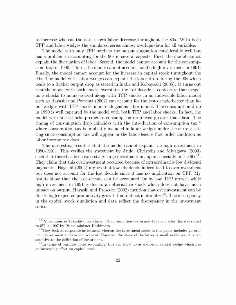
to increase whereas the data shows labor decrease throughout the 80s. With bothTFP and labor wedges the simulated series almost overlaps data for all variables.The model with only TFP predicts the output stagnation considerably well but
has a problem in accounting for the 90s in several aspects. First, the model cannotexplain the �uctuation of labor. Second, the model cannot account for the consump-tion drop in 1990. Third, the model cannot account for the high investment in 1991.Finally, the model cannot account for the increase in capital stock throughout the90s. The model with labor wedges can explain the labor drop during the 90s whichleads to a further output drop as stated in Inaba and Kobayashi (2005). It turns outthat the model with both shocks overstates the lost decade. I conjecture that exoge-nous shocks to hours worked along with TFP shocks in an indivisible labor modelsuch as Hayashi and Prescott (2002) can account for the lost decade better than la-bor wedges with TFP shocks in an endogenous labor model. The consumption dropin 1990 is well captured by the model with both TFP and labor shocks. In fact, themodel with both shocks predicts a consumption drop even greater than data. Thetiming of consumption drop coincides with the introduction of consumption tax16
where consumption tax is implicitly included in labor wedges under the current set-ting since consumption tax will appear in the labor-leisure �rst order condition aslabor income tax does.The interesting result is that the model cannot explain the high investment in
1990-1991. This veri�es the statement by Ando, Christelis and Miyagawa (2003)such that there has been excessively large investment in Japan especially in the 90s17.They claim that this overinvestment occurred because of extraordinarily low dividendpayments. Hayashi (2004) argues that low dividends indeed lead to overinvestmentbut does not account for the lost decade since it has no implication on TFP. Myresults show that the lost decade can be accounted for by low TFP growth whilehigh investment in 1991 is due to an alternative shock which does not have muchimpact on output. Hayashi and Prescott (2002) mention that overinvestment can bedue to high expected productivity growth that did not materialize18. The discrepancyin the capital stock simulation and data re�ect the discrepancy in the investmentseries.
16Prime minister Takeshita introduced 3% consumption tax in mid-1989 and later this was raisedto 5% in 1997 by Prime minister Hashimoto.17They look at corporate investment whereas the investment series in this paper includes govern-
ment investment and current account. However, the share of the latter is small so the result is notsensitive to the de�nition of investment.18In terms of business cycle accounting, this will show up as a drop in capital wedge which has
an increasing e¤ect on capital stock.
22
D Tables and Figures
Table 1. Growth Accounting (% Growth Rates)Yt Kt Lt At
52� 59 7:0 5:1 1:9 3:860� 69 7:7 9:0 �1:6 5:670� 79 3:2 8:2 �1:0 1:180� 89 3:2 3:6 �0:2 2:090� 99 0:7 3:4 �1:2 0:3
Table 2. GNP Component Shares (%)C I
CP CG ID CA52� 59 73:9 63:8 10:1 26:1 25:9 0:260� 69 65:1 57:3 7:9 34:9 34:7 0:270� 79 64:7 55:7 9:0 35:3 34:5 0:880� 89 68:3 58:7 9:6 31:7 29:5 2:290� 99 68:3 58:9 9:5 31:7 29:1 2:5
Table 3. Parameter Values� Discount Factor 0:98� Depreciation Rate 0:116 Consumption-Leisure Parameter 0:32� Capital Share 0:362n Population Growth 0:009 Trend Growth 0:02�z TFP Persistence 0:94�z TFP Volatility 0:027�CDd Labor Shock Persistence 0:975�CDd Labor Shock Volatility 0:031�SGd Labor Shock Persistence 0:801�SGd Labor Shock Volatility 0:030
23
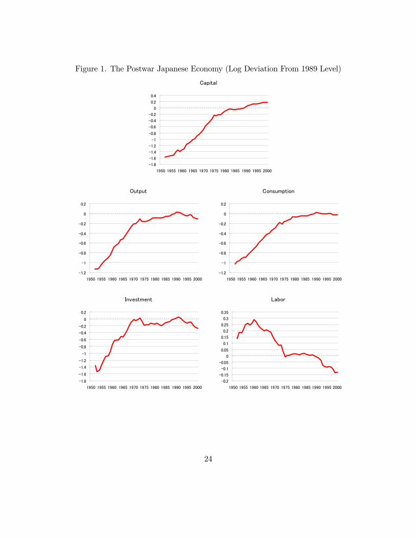
Figure 1. The Postwar Japanese Economy (Log Deviation From 1989 Level)
Capital
1.8
1.6
1.4
1.2
1
0.8
0.6
0.4
0.2
0
0.2
0.4
1950 1955 1960 1965 1970 1975 1980 1985 1990 1995 2000
Output
1.2
1
0.8
0.6
0.4
0.2
0
0.2
1950 1955 1960 1965 1970 1975 1980 1985 1990 1995 2000
Consumption
1.2
1
0.8
0.6
0.4
0.2
0
0.2
1950 1955 1960 1965 1970 1975 1980 1985 1990 1995 2000
Investment
1.8
1.6
1.4
1.2
1
0.8
0.6
0.4
0.2
0
0.2
1950 1955 1960 1965 1970 1975 1980 1985 1990 1995 2000
Labor
0.2
0.15
0.1
0.05
0
0.05
0.1
0.15
0.2
0.25
0.3
0.35
1950 1955 1960 1965 1970 1975 1980 1985 1990 1995 2000
24
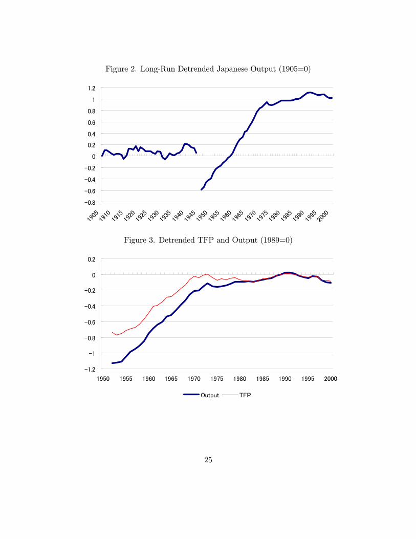
Figure 2. Long-Run Detrended Japanese Output (1905=0)
0.8
0.6
0.4
0.2
0
0.2
0.4
0.6
0.8
1
1.2
1905
1910
1915
1920
1925
1930
1935
1940
1945
1950
1955
1960
1965
1970
1975
1980
1985
1990
1995
2000
Figure 3. Detrended TFP and Output (1989=0)
1.2
1
0.8
0.6
0.4
0.2
0
0.2
1950 1955 1960 1965 1970 1975 1980 1985 1990 1995 2000
Output TFP
25
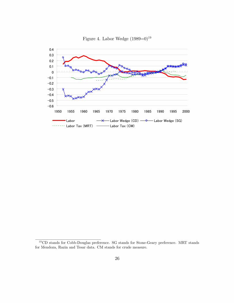
Figure 4. Labor Wedge (1989=0)19
0.6
0.5
0.4
0.3
0.2
0.1
0
0.1
0.2
0.3
0.4
1950 1955 1960 1965 1970 1975 1980 1985 1990 1995 2000
Labor Labor Wedge (CD) Labor Wedge (SG)
Labor Tax (MRT) Labor Tax (CM)
19CD stands for Cobb-Douglas preference. SG stands for Stone-Geary preference. MRT standsfor Mendoza, Razin and Tesar data. CM stands for crude measure.
26
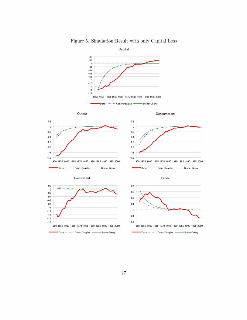
Figure 5. Simulation Result with only Capital Loss
Capital
1.8
1.6
1.4
1.2
1
0.8
0.6
0.4
0.2
0
0.2
0.4
1950 1955 1960 1965 1970 1975 1980 1985 1990 1995 2000
Data CobbDouglas StoneGeary
Output
1.2
1
0.8
0.6
0.4
0.2
0
0.2
1950 1955 1960 1965 1970 1975 1980 1985 1990 1995 2000
Data CobbDouglas StoneGeary
Consumption
1.2
1
0.8
0.6
0.4
0.2
0
0.2
1950 1955 1960 1965 1970 1975 1980 1985 1990 1995 2000
Data CobbDouglas StoneGeary
Investment
1.8
1.6
1.4
1.2
1
0.8
0.6
0.4
0.2
0
0.2
1950 1955 1960 1965 1970 1975 1980 1985 1990 1995 2000
Data CobbDouglas StoneGeary
Labor
0.2
0.1
0
0.1
0.2
0.3
0.4
1950 1955 1960 1965 1970 1975 1980 1985 1990 1995 2000
Data CobbDouglas StoneGeary
27
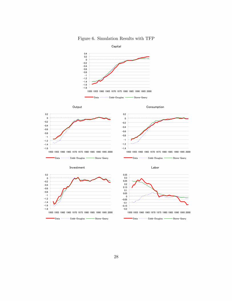
Figure 6. Simulation Results with TFP
Capital
1.8
1.6
1.4
1.2
1
0.8
0.6
0.4
0.2
0
0.2
0.4
1950 1955 1960 1965 1970 1975 1980 1985 1990 1995 2000
Data CobbDouglas StoneGeary
Output
1.6
1.4
1.2
1
0.8
0.6
0.4
0.2
0
0.2
1950 1955 1960 1965 1970 1975 1980 1985 1990 1995 2000
Data CobbDouglas StoneGeary
Consumption
1.4
1.2
1
0.8
0.6
0.4
0.2
0
0.2
1950 1955 1960 1965 1970 1975 1980 1985 1990 1995 2000
Data CobbDouglas StoneGeary
Investment
1.8
1.6
1.4
1.2
1
0.8
0.6
0.4
0.2
0
0.2
1950 1955 1960 1965 1970 1975 1980 1985 1990 1995 2000
Data CobbDouglas StoneGeary
Labor
0.2
0.15
0.1
0.05
0
0.05
0.1
0.15
0.2
0.25
0.3
0.35
1950 1955 1960 1965 1970 1975 1980 1985 1990 1995 2000
Data CobbDouglas StoneGeary
28
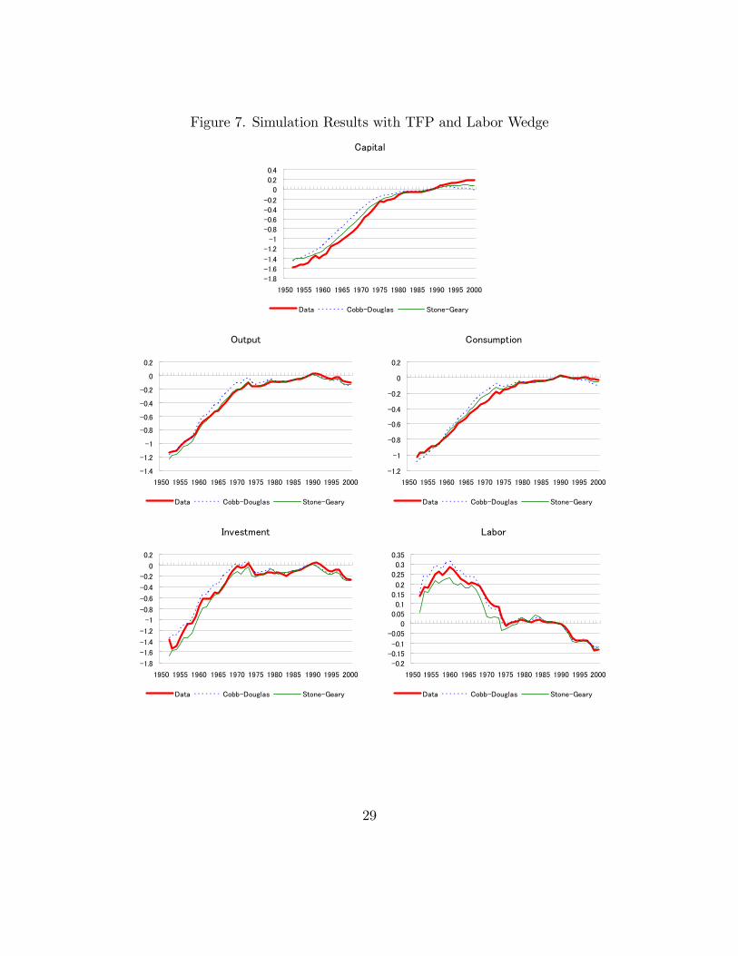
Figure 7. Simulation Results with TFP and Labor Wedge
Capital
1.8
1.6
1.4
1.2
1
0.8
0.6
0.4
0.2
0
0.2
0.4
1950 1955 1960 1965 1970 1975 1980 1985 1990 1995 2000
Data CobbDouglas StoneGeary
Output
1.4
1.2
1
0.8
0.6
0.4
0.2
0
0.2
1950 1955 1960 1965 1970 1975 1980 1985 1990 1995 2000
Data CobbDouglas StoneGeary
Consumption
1.2
1
0.8
0.6
0.4
0.2
0
0.2
1950 1955 1960 1965 1970 1975 1980 1985 1990 1995 2000
Data CobbDouglas StoneGeary
Investment
1.8
1.6
1.4
1.2
1
0.8
0.6
0.4
0.2
0
0.2
1950 1955 1960 1965 1970 1975 1980 1985 1990 1995 2000
Data CobbDouglas StoneGeary
Labor
0.2
0.15
0.1
0.05
0
0.05
0.1
0.15
0.2
0.25
0.3
0.35
1950 1955 1960 1965 1970 1975 1980 1985 1990 1995 2000
Data CobbDouglas StoneGeary
29
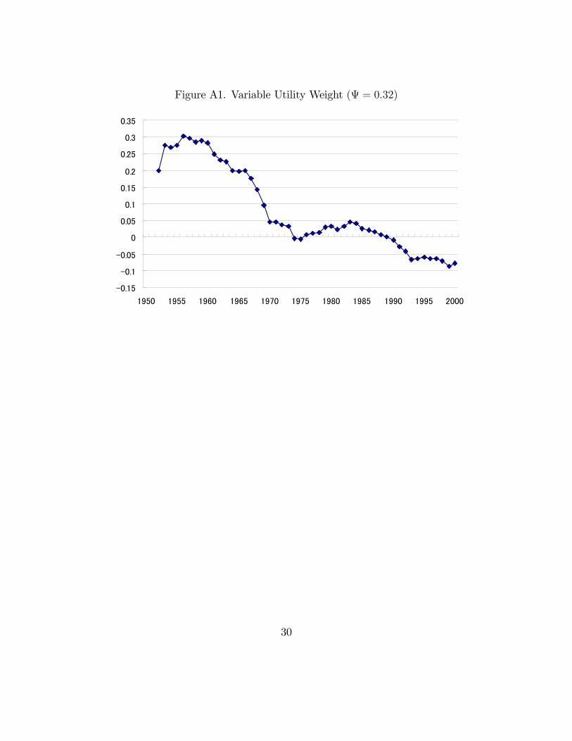
Figure A1. Variable Utility Weight ( = 0:32)
0.15
0.1
0.05
0
0.05
0.1
0.15
0.2
0.25
0.3
0.35
1950 1955 1960 1965 1970 1975 1980 1985 1990 1995 2000
30
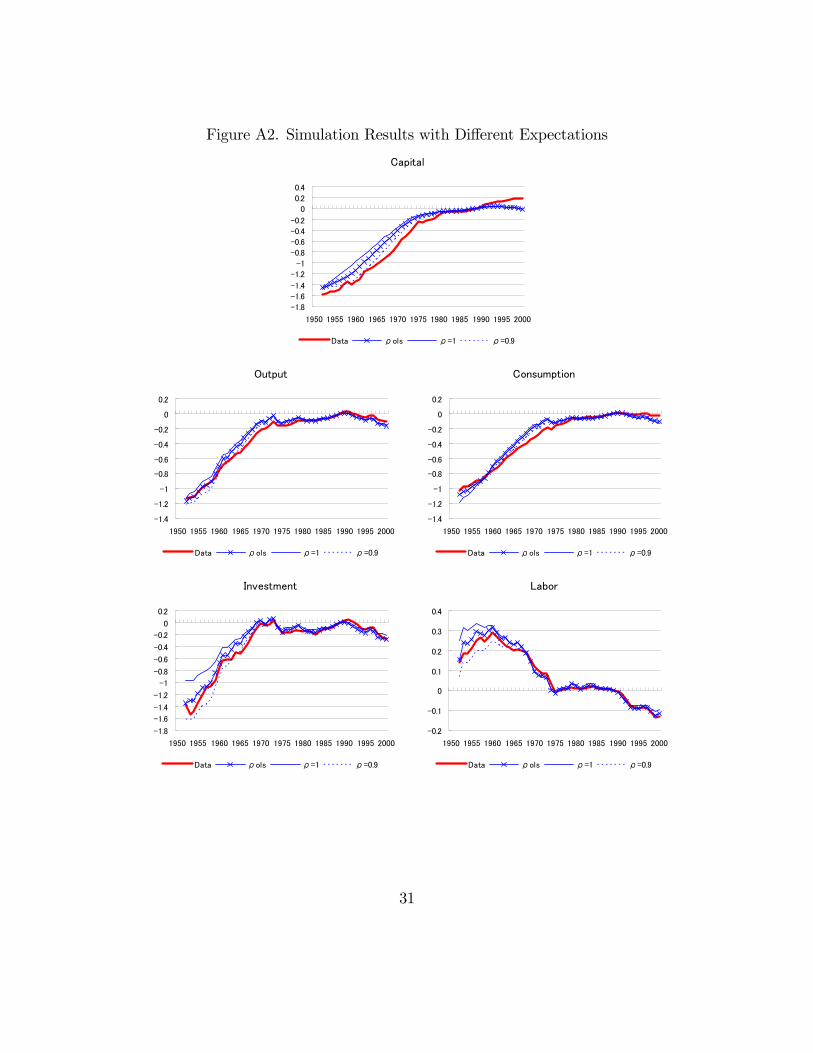
Figure A2. Simulation Results with Di¤erent Expectations
Capital
1.8
1.6
1.4
1.2
1
0.8
0.6
0.4
0.2
0
0.2
0.4
1950 1955 1960 1965 1970 1975 1980 1985 1990 1995 2000
Data ρols ρ=1 ρ=0.9
Output
1.4
1.2
1
0.8
0.6
0.4
0.2
0
0.2
1950 1955 1960 1965 1970 1975 1980 1985 1990 1995 2000
Data ρols ρ=1 ρ=0.9
Consumption
1.4
1.2
1
0.8
0.6
0.4
0.2
0
0.2
1950 1955 1960 1965 1970 1975 1980 1985 1990 1995 2000
Data ρols ρ=1 ρ=0.9
Investment
1.8
1.6
1.4
1.2
1
0.8
0.6
0.4
0.2
0
0.2
1950 1955 1960 1965 1970 1975 1980 1985 1990 1995 2000
Data ρols ρ=1 ρ=0.9
Labor
0.2
0.1
0
0.1
0.2
0.3
0.4
1950 1955 1960 1965 1970 1975 1980 1985 1990 1995 2000
Data ρols ρ=1 ρ=0.9
31
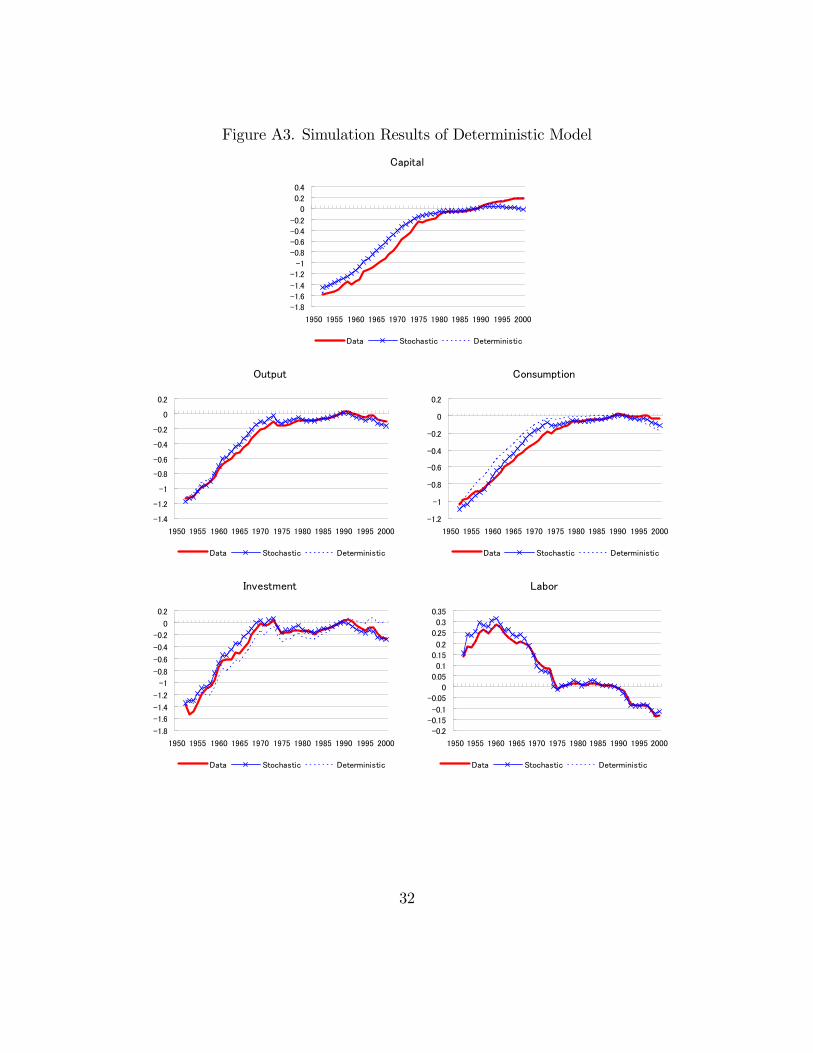
Figure A3. Simulation Results of Deterministic Model
Capital
1.8
1.6
1.4
1.2
1
0.8
0.6
0.4
0.2
0
0.2
0.4
1950 1955 1960 1965 1970 1975 1980 1985 1990 1995 2000
Data Stochastic Deterministic
Output
1.4
1.2
1
0.8
0.6
0.4
0.2
0
0.2
1950 1955 1960 1965 1970 1975 1980 1985 1990 1995 2000
Data Stochastic Deterministic
Consumption
1.2
1
0.8
0.6
0.4
0.2
0
0.2
1950 1955 1960 1965 1970 1975 1980 1985 1990 1995 2000
Data Stochastic Deterministic
Investment
1.8
1.6
1.4
1.2
1
0.8
0.6
0.4
0.2
0
0.2
1950 1955 1960 1965 1970 1975 1980 1985 1990 1995 2000
Data Stochastic Deterministic
Labor
0.2
0.15
0.1
0.05
0
0.05
0.1
0.15
0.2
0.25
0.3
0.35
1950 1955 1960 1965 1970 1975 1980 1985 1990 1995 2000
Data Stochastic Deterministic
32
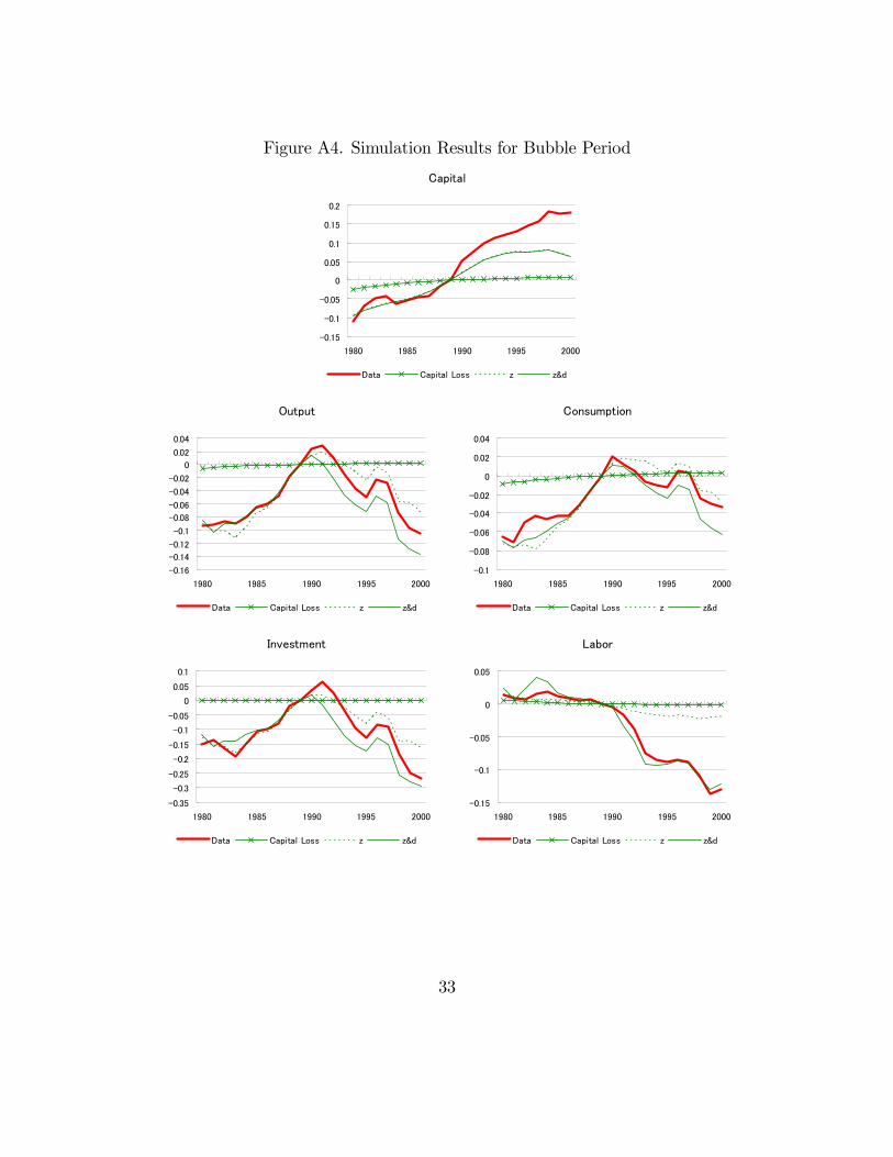
Figure A4. Simulation Results for Bubble Period
Capital
0.15
0.1
0.05
0
0.05
0.1
0.15
0.2
1980 1985 1990 1995 2000
Data Capital Loss z z&d
Output
0.16
0.14
0.12
0.1
0.08
0.06
0.04
0.02
0
0.02
0.04
1980 1985 1990 1995 2000
Data Capital Loss z z&d
Consumption
0.1
0.08
0.06
0.04
0.02
0
0.02
0.04
1980 1985 1990 1995 2000
Data Capital Loss z z&d
Investment
0.35
0.3
0.25
0.2
0.15
0.1
0.05
0
0.05
0.1
1980 1985 1990 1995 2000
Data Capital Loss z z&d
Labor
0.15
0.1
0.05
0
0.05
1980 1985 1990 1995 2000
Data Capital Loss z z&d
33