imes discussion paper series - bank of japan discussion paper series 2003-e-7 july 2003 on the risk...
TRANSCRIPT

IMES DISCUSSION PAPER SERIES
INSTITUTE FOR MONETARY AND ECONOMIC STUDIES
BANK OF JAPAN
C.P.O BOX 203 TOKYO
100-8630 JAPAN
You can download this and other papers at the IMES Web site:
http://www.imes.boj.or.jp
Do not reprint or reproduce without permission.
On the Risk Capital Framework of FinancialInstitutions
Tatsuya Ishikawa, Yasuhiro Yamai, Akira Ieda
Discussion Paper No. 2003-E-7

NOTE: IMES Discussion Paper Series is circulated in
order to stimulate discussion and comments. Views
expressed in Discussion Paper Series are those of
authors and do not necessarily reflect those of
the Bank of Japan or the Institute for Monetary
and Economic Studies.

IMES Discussion Paper Series 2003-E-7
July 2003
On the Risk Capital Framework of Financial Institutions
Tatsuya Ishikawa*, Yasuhiro Yamai**, Akira Ieda***
Abstract
In this paper, we consider the risk capital framework adopted by financial institutions.
Specifically, we review the recent literature on this issue, and clarify the economic
assumptions behind this framework. Based on these observations, we then develop a
simple model for analyzing the economic implications of this framework.
The main implications are as follows. First, risk capital allocations are theoretically
unnecessary without deadweight costs for raising capital, which are not usually assumed
in the business practices of financial institutions. Second, the risk-adjusted rate of
return is redundant as it provides no additional information beyond the net present value.
Third, risk capital allocation is intrinsically difficult because it is hard to incorporate the
correlations among asset returns.
Key words: Risk capital, risk management, capital structure, capital budgeting, risk-adjusted rate of return, capital allocation, deadweight cost.
JEL classification: G20
* Research Division 1, Institute for Monetary and Economic Studies, Bank of Japan (currently RiskManagement Department, UFJ Holdings, Inc.) (E-mail: [email protected])
** Research Division 1, Institute for Monetary and Economic Studies (currently Bank Examinationand Surveillance Department), Bank of Japan (E-mail: [email protected])
*** Research Division 1, Institute for Monetary and Economic Studies, Bank of Japan (E-mail:[email protected])
The views expressed here are those of the authors and do not necessarily reflect those of the Bank of
Japan, the Institute for Monetary and Economic Studies, the Bank Examination and Surveillance
Department or UFJ Holdings, Inc.

1
1. Introduction
In recent years, an increasing number of financial institutions have adopted risk
capital frameworks1. Under these frameworks, banks determine the amount of capital
needed to cover their risk, and measure their risk-adjusted performance. According to
Zaik et al.[1996], James[1996], and Matten[2000], the elements of the risk capital
frameworks adopted by financial institutions are as follows.
(i) Holding sufficient capital to cover risk Financial institutions hold a sufficient amount of capital to cover the risk of
their business activities (this capital is called “risk capital”). They determine the
amount of risk capital as the unexpected losses of their operations. They
measure the unexpected losses using value-at-risk and other risk measures.
(ii) Allocating risk capital to each operating division Financial institutions allocate risk capital to individual lines of business
according to their respective risks.
(iii) Evaluating profitability based on risk-adjusted rates of return Financial institutions evaluate the performance of individual lines of business
using their respective “risk-adjusted rates of return” (profit divided by allocated
risk capital).
In this paper, we call this framework the “standard framework” of risk capital and
consider its economic implications. We consider this framework as the representative
example of risk capital frameworks, since it is both typical and common to the business
practices of financial institutions2.
This standard framework assumes that financial institutions are risk-averse decision-
makers and make investment decisions based on risk-return tradeoffs. However,
finance theory does not assume, a priori, that financial institutions are risk-averse
decision-makers. Rather, finance theory says that a firm is primarily a nexus of
1 The “risk capital framework” characterized here is also called “integrated risk management” or the
“RAROC system.”2 There are several variations to this framework. See Zaik et al.[1996], James[1996], and
Matten[2000].

2
contracts, and that a firm is risk-neutral in a perfect market (Modigliani and Miller
[1958]). Therefore, to justify the risk capital framework from the theoretical viewpoint,
we have to establish the reason why financial institutions are risk-averse.
Since the 1990s, a number of research papers have addressed this issue3 from the
viewpoint of finance theory. They establish how and why financial institutions are
risk-averse and propose risk capital frameworks that are well aligned with their
economic analyses.
In this paper, we consider the risk capital framework generally adopted at financial
institutions. Specifically, we review the recent literature and clarify the economic
assumptions behind this framework. Based on these observations, we then develop a
simple model for analyzing the economic implications of this framework.
The main findings are as follows.
• The allocation of risk capital is theoretically unnecessary when we do not assume the
deadweight costs of raising capital. As the deadweight costs of raising capital are
not usually assumed in the business practices of financial institutions, the allocation of
risk capital seems unnecessary for practical use.
• The risk-adjusted rate of return in the standard framework is equivalent to the net
present value. The risk-adjusted rate of return is inferior to the net present value
since the former requires the calculation of risk capital (i.e. value-at-risk) while the
latter does not.
• The allocation of risk capital is intrinsically difficult as we have to consider the
correlations among asset returns.
In the first half of this paper (through Section 3), we describe the theories presented
in the prior research on risk capital. In Section 2, we consider a firm’s financing
3 Froot and Stein[1998] examine the capital of financial institutions explicitly incorporating the
concavity of the payoff under the existence of economic friction. Merton and Perold[1993] argue
that risk capital is viewed as insurance purchased as required against bankruptcy. Crouhy,
Turnbull, and Wakeman[1999] define risk capital as the risk-free assets required to restrain the
probability of bankruptcy to within a certain level, and primarily address capital budgeting
decision-making problems.

3
decision-making in a perfect market. In a perfect market, the Modigliani-Miller
proposition holds and risk capital plays no role in financing decision-making. In
Section 3, we introduce economic friction such as bankruptcy costs and information
asymmetry. With economic friction, a firm becomes risk-averse and risk capital plays
some roles. We also note that economic friction is more serious for financial
institutions than for non-financial firms. Thus, risk capital plays greater roles at
financial institutions than at other firms.
In the second half of this paper (from Section 4 onward), we develop a simple model
for analyzing the standard framework. From this model, we derive the economic
implications of the risk capital framework in Section 4, and then consider the difficulty
of risk capital allocation in Section 5.
2. Financing Decisions in a Perfect Market
In this section, we describe a firm’s4 capital structure, risk management and capital
budgeting under a perfect market5. This description prepares for the discussions of
risk capital in subsequent sections.
(1) The Modigliani-Miller Proposition
The Modigliani-Miller proposition (hereafter the “MM proposition”), stated in
Modigliani and Miller[1958], is the most important for considering a firm’s capital
structure in a perfect market. Based on the MM proposition, Fama[1978]
demonstrates that in a perfect market that satisfies the following conditions, how firms
raise funds has no influence on their value.
(i) Frictionless market (there are no transaction costs or taxes, and all assets are
perfectly divisible and marketable)
4 We make no distinctions between financial institutions and non-financial firms in this section as we
only consider the decision-making in a perfect market.5 See Brealey and Myers[2000], McKinsey & Company Inc., et al.[2000], and Damodaran[1999] for
firms’ financing decision-making in a perfect market.

4
(ii) Information efficiency (all investors, firms and firms’ managers have the same
information, and hold homogeneous expectations regarding how this information
will affect market prices)
(iii) Given investment decisions (the investment decisions are given conditions, and
are completely independent from the decisions on raising new external funds)
(iv) Equal access (all market participants can issue securities under the same terms)
The essence of the MM proposition is that a firm’s capital structure does not matter
because investors can arrange their own desired payoffs by adjusting their portfolios by
themselves.
The MM proposition also says that a firm’s risk management does not matter in a
perfect market. A firm has no need to hedge the tradable risks it is exposed to because
the investors who invest in its stocks or bonds can hedge the firm’s risks by trading
those risks by themselves. So, in a perfect market where the MM proposition holds,
one cannot assume, a priori, that a firm is risk-averse.
In the following subsections, we explicate the firm’s decision-making in a perfect
market, where the MM proposition holds, using the asset pricing model.
(2) Asset Pricing
To examine how risk management and capital structure affect the firm’s value, we
need to calculate the present value of the firm’s future payoff (hereafter “the firm’s
value”). In this paper, we adopt the Capital Asset Pricing Model (CAPM6) to
determine the present value of the future uncertain payoff.
We adopt a two-period model (Period 0 and Period 1). Under CAPM, Equation (1)shows the relationship between the rate of return ir for a given asset i and the rate of
return for the market portfolio (the market return).7
6 The argument in this paper could also be developed using a wider class of pricing models that
can be nested in the stochastic discount factor model. See Cochrane [2001] for the details of the
stochastic discount factor.7 ][•E represents the expectation operator with the given information at period 0.

5
)][(][ fMifi rrErrE −+= β , (1)
where8, )var(
),cov(
M
Mii r
rr=β ,
Mr : market return,
fr : risk-free rate,
iβ is a constant for each asset.
Here, the random variable iX indicates the asset’s payoff at Period 1, and )( iXP
indicates the asset’s present value at Period 0. By definition of ir ,
)(][
][1i
ii XP
XErE =+ . (2)
Substituting Equation (2) into Equation (1), and using )var(/)][( MfM rrrE −≡γ
which is not dependent on the characteristics of each asset, the value of )( iXP is then
determined as shown in Equation (3).
f
Miii r
rXXEXP+
−=1
),cov(][)( γ . (3)
(3) Capital Budgeting, Capital Structure and Risk Management in a PerfectMarket
Next, we explain a firm’s financing decision-making (capital budgeting, capital
structure, and risk management) in a perfect market, where the MM proposition holds.
In this paper, capital budgeting, capital structure and risk management decision-making
are defined as follows.
Capital Budgeting
To decide how much to invest in an investment opportunity.
Capital Structure
To select how the investment is financed. For simplicity, we assume that a firm
8 ),cov( YX expresses the covariance of the random variables X and Y , and )var(X expresses
the variance of the random variable X .

6
can finance only with common stocks and straight bonds.
Risk Management
To decide whether or not to hedge the tradable risks that a firm is exposed to.
In this paper, those three decisions are collectively referred to as the firm’s “financing
decision-making.”
The firm’s Net Present Value (NPV) is expressed by Equation (4) where )(XP
represents the firm’s present value and I represents the amount of capital.
IXPNPV −= )( . (4)
One of the most important characteristics of a firm’s financing decision-making in a
perfect market is “value additivity”.9 The concept of value additivity is as follows.Suppose there are two investment opportunities A and B with payoffs AX and BX ,
respectively, and their present values are )( AXP and )( BXP . Value additivity holds
when the sum of these present values is the same as the present value of the twoinvestment opportunities taken together, that is where )()()( BABA XPXPXXP +=+ .
From Equation (3), value additivity holds when the following holds.
f
MBABABA r
rXXXXEXXP+
+−+=+
1),cov(][
)(γ
f
MBB
f
MAA
rrXXE
rrXXE
+−
++
−=
1),cov(][
1),cov(][ γγ
)()( BA XPXP += . (5)
Value additivity results from the linearity of the present value )(XP to the payoff X .
Additionally, because BABA III +=+ , the NPV is also value additive as shown in
Equation (6).
})({})({ BBAABA IXPIXPNPVNPV −+−=+
}{)}()({ BABA IIXPXP +−+=
}{)( BABA IIXXP +−+=
BANPV += . (6)
9 See Brealey and Myers[2000] for a detailed introduction to value additivity.

7
This value additivity has the following important implications for the firm’s financing
decision-making.
Capital Budgeting
The capital budgeting decisions on multiple investment opportunities are
independent of each other when value additivity holds. As is clear from Equation
(6)10, the NPV of one investment opportunity is independent of the NPV of another
investment opportunity. For example, suppose that a firm has two operating
divisions, and they both implement capital budgeting. If each division
independently maximizes its NPV without any consideration for the other, the NPV
of the firm will also be maximized.
Capital Structure
Value additivity is equivalent to the MM proposition that capital structure does
not matter. This can be shown as follows.11 Let a random variable X indicate a
firm’s payoff at Period 1. When the firm’s only means of fundraising is theissuance of stocks, the firm’s value becomes )(1 XPP = . Next, consider the firm’s
value when the firm can raise funds by issuing stocks and/or bonds. When the
stock and bond payoffs at Period 1 are S and D , respectively, the firm’s presentvalue 2P is the sum of those of the stocks and bonds, so )()(2 DPSPP += . As
the firm’s overall payoff at Period 1 can be divided into those of stocks and bonds,
DSX += . Because of the value additivity, it can then be demonstrated that
21 PP = , as in Equation (7).
21 )()()()( PDPSPDSPXPP =+=+== . (7)
10 Rather than utilizing Equation (3), practitioners commonly calculate the present value using a
modified version of Equation (2): ( iii rXEXP += 1/)()( ). In this case, though it is necessary to
calculate the value of ir (or iβ ) for each investment opportunity, a single value is often adopted
for an entire firm. If the individual investment opportunity’s β were always equal to (or nearly
equal to) the firm’s β , this would not present many problems. Since this is not the case, the use
of the ( iii rXEXP += 1/)()( ) equation is generally inappropriate, as detailed below.11 See Ross[1978] for this proof of the MM proposition.

8
Risk Management
Value additivity is equivalent to the irrelevance of risk management12. This can
be shown by the following example. Let a random variable X indicate a firm’s
payoff at Period 1. Suppose that the variability of the firm’s payoff X can all be
hedged by market trading, specifically by a forward contract of the payoff’s
underlying assets. In a perfect market, the NPV of the forward contract ( XF − ,
where the forward delivery price is F ) is zero.13 In other words, Equation (3) can
be restated as follows.
f
M
rrXFXFE
+−−−
=1
),cov(][0
γ. (8)
Thus, the forward delivery price F can be expressed as follows.14
),cov(][ MrXXEF γ−= . (9)
Here, after the risk on the payoff X is hedged and the payoff becomes the forwarddelivery price F , the firm’s value after the hedge 1P′ becomes identical to the
firm’s value before the hedge )(XP .
f
M
ff
M
rrXXE
rF
rrFFEFPP
+−
=+
=+
−==′
1),cov(][
11),cov(][
)(1γγ
)(XP= . (10)
Therefore, because of the value additivity, the firm’s hedge operation does not
12 See Culp[2001] for a more detailed explanation.13 In a perfect market, the NPV of market trading is always zero. This can be explained as follows.
Assume a given trading opportunity with a positive NPV in a perfect market. Because all the
participants can freely engage in trading, they would all take advantage of this trading opportunity.
This would result in a surplus demand for this trading opportunity, so the market price would then
move downward, reducing the NPV. This market price adjustment would continue until the NPV
declines to zero, and reach equilibrium when the NPV equals zero. In a perfect market, this price
adjustment would be done instantaneously. Thus market trading with a positive NPV cannot exist
in a perfect market.14 From Equation (3), ),cov()()1(][ Mf rXXPrXE γ++= , so )()1( XPrF f+= . This is
the forward delivery price derived from the non-arbitrage conditions whereby there are no risk-free
profits.

9
change its value. Thus, risk management is irrelevant when value additivity holds.
3. Financing Decisions in a Real Market
(1) Existence of Economic Friction
In the previous section, we assumed a perfect market. In a perfect market, value
additivity holds and capital structure and risk management are irrelevant. As shown in
the previous section, value additivity is based on the linear relationship between the
NPV and the payoff. Thus, the irrelevance of capital structure and risk management
depend on this linear relationship.
In the real world, the firm’s NPV may not be a linear function of the payoff. This is
usually due to the existence of “economic friction”15 such as bankruptcy costs and
progressive corporate tax rates. This friction places costs on the firm that have a
convex function with the payoff.
When the payoff before considering the costs of economic friction is X and thepayoff after considering the costs is )(XV , there is a concave function between )(XV
and X , as shown in the following figures. The firm’s NPV is no longer linear with its
payoff, and the MM proposition and value additivity no longer hold.
15 Although the agency problem is also an important reason for the imperfection of financial markets,
it is not addressed in this paper. See Barnea, Haugen, and Senbet[1985] for the details of the
agency problem.

10
Figures: Relation between costs from economic friction and payoff
P a y o ff p rio r to c o n s id e r in g e co n o m ic f r ic tio n co s ts : X
C o s ts F ro m E co n o m ic F ric tio n
P ay o ff p r io r to co n s id e rin g eco n o m ic f ric tio n co s ts : X
P ay o ff a fte r co n s id e rin g eco n o m ic fric tio n co s ts :V (X )
P ay o ff in a co m p le te m ark et ( lin ea rfu n c tio n V (X )= X )
P ay o ff co n s id e rin g eco n o m ic fric tio nco sts
The following three costs have been noted as types of economic friction that affect
the linearity of NPVs (Smith and Stulz[1985], Froot, Scharfstein, and Stein[1993]).
(i) Corporate taxes
If effective marginal tax rates on a firm are progressive, or an increasing function
of the firm’s pre-tax value, the after-tax value of the firm is a concave function of its
pre-tax value.
(ii) Bankruptcy costs
A firm has to pay bankruptcy costs,16 such as legal and administrative costs, when
16 There are two types of bankruptcy costs: direct and indirect. The direct costs of bankruptcy are
the costs of processing bankruptcy procedures such as legal and administrative costs. The indirect
costs of bankruptcy include the costs of deterioration of the firm’s business from the bankruptcy
procedure. See Brealey and Myers[2000] for details of bankruptcy costs.
11
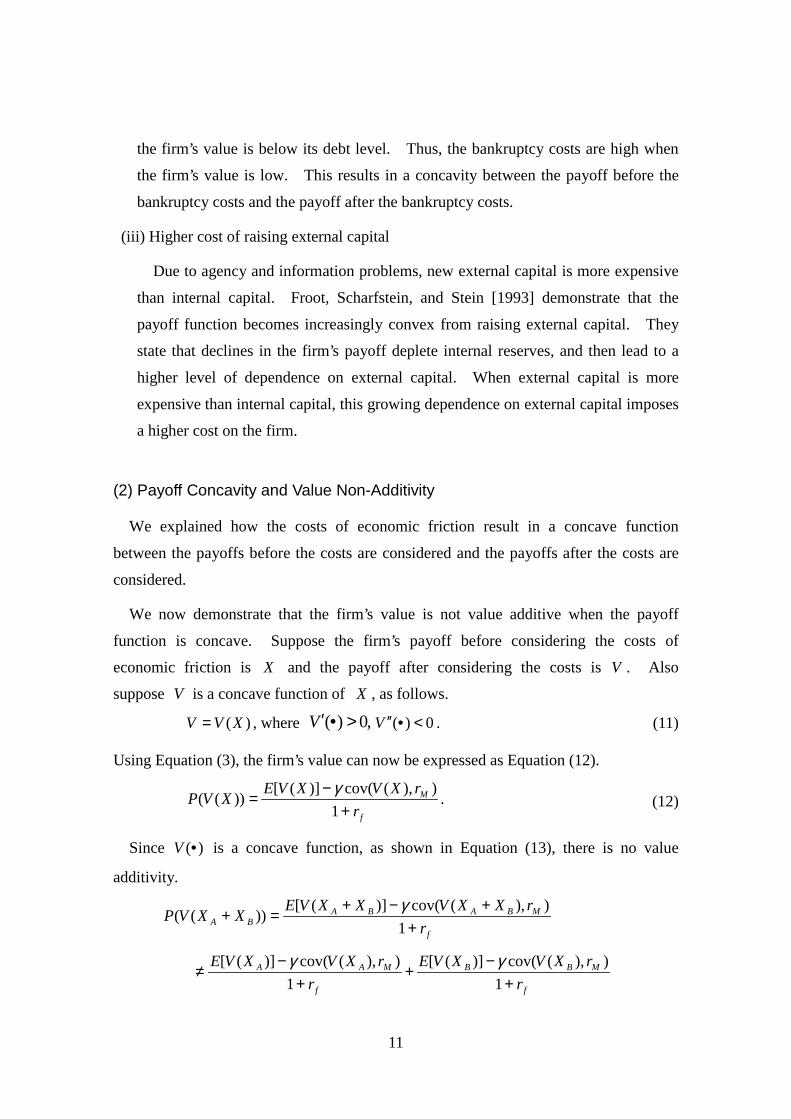
the firm’s value is below its debt level. Thus, the bankruptcy costs are high when
the firm’s value is low. This results in a concavity between the payoff before the
bankruptcy costs and the payoff after the bankruptcy costs.
(iii) Higher cost of raising external capital
Due to agency and information problems, new external capital is more expensive
than internal capital. Froot, Scharfstein, and Stein [1993] demonstrate that the
payoff function becomes increasingly convex from raising external capital. They
state that declines in the firm’s payoff deplete internal reserves, and then lead to a
higher level of dependence on external capital. When external capital is more
expensive than internal capital, this growing dependence on external capital imposes
a higher cost on the firm.
(2) Payoff Concavity and Value Non-Additivity
We explained how the costs of economic friction result in a concave function
between the payoffs before the costs are considered and the payoffs after the costs are
considered.
We now demonstrate that the firm’s value is not value additive when the payoff
function is concave. Suppose the firm’s payoff before considering the costs of
economic friction is X and the payoff after considering the costs is V . Also
suppose V is a concave function of X , as follows.
)(XVV = , where ,0)( >•′V 0)( <•′′V . (11)
Using Equation (3), the firm’s value can now be expressed as Equation (12).
f
M
rrXVXVEXVP
+−
=1
)),(cov()]([))((
γ. (12)
Since )(•V is a concave function, as shown in Equation (13), there is no value
additivity.
f
MBABABA r
rXXVXXVEXXVP+
+−+=+
1)),(cov()]([
))((γ
f
MBB
f
MAA
rrXVXVE
rrXVXVE
+−
++
−≠
1)),(cov()]([
1)),(cov()]([ γγ

12
))(())(( BA XVPXVP += . (13)
Because there is no value additivity, the conclusions reached for firm’s financing
decision-making in a perfect market no longer hold. In other words, the firm’s
financing decision-making in a real market is far more complex compared with that in a
perfect market.
(3) Economic Friction at Financial Institutions
Thus far, we have made no distinction between financial institutions and non-
financial firms. However, economic friction has a greater influence on financial
institutions than on non-financial firms. Merton and Perold[1993] note that
bankruptcy costs and information costs are more remarkable at financial institutions
than at non-financial firms.
(i) Bankruptcy costs
The major customers of financial institutions can be major liability holders; for
example, policyholders, depositors, and swap counterparties are all liability holders
as well as customers. When the bankruptcy risk at a financial institution rises,
customers typically move to other financial institutions. This exodus of customers
imposes another indirect cost on the struggling financial institution, because it loses
the profits that would otherwise have been derived.
An exodus of customers may also occur at non-financial firms, but the impact is
far greater at financial institutions because their customers, especially those who are
outside of the deposit insurance safety net, are extremely sensitive to bankruptcy
risk. Thus, the bankruptcy costs at financial institutions17 are far greater than those
at non-financial firms.
(ii) Information costs
In general, financial institutions do not disclose their assets or activities in great
detail, and thus their business appears opaque to customers and investors.18 That is,
17 See Merton[1997] for a discussion of the scale of bankruptcy costs at financial institutions.18 The “opaqueness” of financial institutions is first noted in Ross[1989].
13
the detailed asset holdings and business activities of the firm are not publicly
disclosed (or, if disclosed, only with a considerable lag in time). Furthermore,
principal financial firms typically have relatively liquid balance sheets that, in the
course of just weeks, can and often do undergo substantial changes in size and risk.
The information asymmetry between the management of financial institutions and
outsiders leads to the problem of higher costs of raising external capital (Myers and
Majluf[1984]). As a result, the problem of higher costs of raising external capital
is more serious at financial institutions than at non-financial firms.
Froot and Stein [1998] develop a framework for analyzing the capital allocation and
capital structure decisions of financial institutions incorporating economic friction. In
their framework, they propose a two-factor model that can be used for capital budgeting
problems at financial institutions. With the model, they clarify the roles of economic
friction on the financing decision-making of financial institutions.
However, the framework of Froot and Stein [1998] is not widely adopted in the
practices of financial institutions. As they note, their framework requires calculationof the concavity of the payoff function ( )(•V in equation (11)), which is hard to measure
in practice. Instead, financial institutions adopt risk capital frameworks, which are not
consistent with the framework of Froot and Stein [1998].
In the next chapter, we consider the risk capital frameworks adopted by financial
institutions.
4. Standard Framework
In this section, we analyze the risk capital frameworks adopted by financial
institutions. As noted in the Introduction, we use the “standard framework” as a
generalized example of the risk capital frameworks. The elements of the standard
framework are as follows.
(i) Holding sufficient capital to cover risk Financial institutions hold a sufficient amount of capital to cover the risk of
their business activities (this capital is called “risk capital”). They determine the
amount of risk capital as the unexpected losses of their operations. They
measure the unexpected losses using value-at-risk and other risk measures.

14
(ii) Allocating risk capital to each operating division Financial institutions allocate risk capital to individual lines of business
according to their respective risks.
(iii) Evaluating profitability based on risk-adjusted rates of return Financial institutions evaluate the performance of individual lines of business
using their respective “risk-adjusted rates of return” (profit divided by allocated
risk capital).
In this section, we first demonstrate how the standard framework can be developed
into a model (hereinafter, “the standard model”) by positing assumptions that simplify
the firm’s payoff. We then examine the economic implications of the standard
framework of risk capital adopted by financial institutions.
Also, we limit our considerations of the standard framework in this section to elements
(i) “holding sufficient risk capital to cover risk” and (iii) “evaluating profitability based
on risk-adjusted rates of return.” We proceed with considerations of element (ii)
“allocating risk capital to each operating division” in the subsequent section.
(1) Basic Concept of the Standard Framework
The basic concept of the standard framework is “holding sufficient risk capital to
cover risk.” More precisely, the risk is quantified using value-at-risk or other risk
measures and capital equal to or greater than the calculated risk is held as a buffer
against it.
(2) Standard Model
We develop the standard model based on the setup presented by Froot and
Stein[1998], as follows. The model has two time periods, Period 0 and Period 1. We
assume that a financial institution invests in an investment opportunity that will
generate a per-unit payoff of X at Period 1. At period 0, X is a random variablewith a mean of µ . Note that we do not have to assume that X obeys a normal
distribution. We also assume that this investment opportunity is available for an
infinite number of units and that the investment can be implemented without cost.

15
Meanwhile, this financial institution raises an amount of capital K at Period 0, and
invests the proceeds in a risk-free asset. The following discussions through subsection
(5) all assume this amount of capital K is exogenously given.
The financial institution makes an investment of α units in the investment
opportunity. Now, we introduce the standard framework whereby the institution
retains sufficient capital to cover the risk. In this paper, we assume the linearhomogeneity presented in Equation (14) for the amount of risk )(•ρ .
)()( XX αραρ = . (14)
The financing decision-making of the institution takes place under the restrictions
expressed by Equation (15).
KX ≤)(αρ . (15)
Equation (15) may be viewed as a function expressing the financial institution’s
“behavioral principle” under the standard framework of risk capital whereby the risk
may not exceed the risk capital. We assume that the payoff for this financial
institution is as expressed in Equations (16) and (17).
. when KXwwV ≤= )(,)( αρ (16)
KrXw f )1( ++=α . (17)
Equation (16) says that economic friction is nonexistent as long as the capital covers
the risk of the financial institution. This is the basic principle of the standard
framework19. Given the linear homogeneity, Equation (15) can be rewritten as
follows.
)(XK
ρα ≤ . (18)
The institution’s NPV can now be expressed as follows based on Equations (16) and
(17).
19 Some may argue that the standard framework of risk capital assumes a convex function for a
firm’s value. If we assume a convex function, however, the firm’s financing decision-making
would be the same as that in Froot and Stein [1998], which is not widely adopted by financial
institutions.

16
Kr
rwwEKwPKwVPNPVf
M −+
−=−=−=
1),cov(][
)())((γ
Kr
rKrXKrXE
f
Mff −+
++−++=
1),)1(cov(])1([ αγα
f
M
f
Mf
rrXXEK
rrXKrXE
+−
=−+
−++=
1),cov(][
1),cov()1(][ γα
αγα
)(XPα= . (19)
As long as the inequality of Equation (15) holds, the NPV has nothing to do with the
capital K , and is equal to the present value of the investment in α units. Thus, the
financial institution’s NPV has value additivity.
(3) Capital Budgeting under a Single Investment Opportunity
Under the standard model, the capital budgeting is very simple. When the
institution is holding capital K , the objective is to maximize the NPV as calculated by
Equation (19) under the restrictions imposed by Equation (15). This can be expressed
as Equation (20).
)(max XPαα
, subject to )(XK ρα ≤ . (20)
The solution to this maximization problem is clearly )(XK ρα = , so the
maximized NPV becomes )()( XXKPNPV ρ= .
Moreover, the decision on whether or not to invest in any given investment
opportunity is simply determined by whether or not its NPV is positive. In otherwords, as long as 0)( >XP , the investment will increase the financial institution’s
NPV (see Equation (19)) and should therefore be implemented. Meanwhile the
investment amount α is determined by Equation (18).
The expression 0)( >XP can be reformulated into the following expression.
0)( >XP )][()var(
),cov(][ fM
M
M rrEr
rXXE −>⇔ , (21)
(Multiplying both sides by K/α and adding fr )

17
)][(][/, fMKXCAPMf rrEr
KKwE −+>−⇔ αβ , (22)
where )var(),cov(, MMKXCAPM rrKXαβ α = .
The left-hand side of Equation (22) now expresses the expected rate of return on the
capital K , and the right-hand side expresses the shareholders’ expected rate of return
calculated using the CAPM. Thus, Equation (22) is an expression of the risk-adjusted
rates of return approach often adopted by financial institutions. The right-hand side of
Equation (22) is often called the “hurdle rate”. Equation (22) shows that this standard
model well describes the standard risk capital framework of financial institutions.
However, notably, the capital budgeting determined by Equation (22) is not
dependent on the capital K . This is because Equation (22) is equivalent to Equation
(21), which is not dependent on the capital K . It indicates that an investment should
be made whenever the NPV of the investment opportunity is positive. Therefore, the
risk-adjusted rate of return derived from Equation (22), which is widely used for capital
budgeting, provides no additional information to the capital budgeting based solely on
present value.
(4) Risk Management
The influence of risk management on firm’s value can also easily be analyzed.
From the conclusions of subsection (3), the maximized NPV of the financial
institution can be expressed as follows.
)()(
XXKPNPV
ρ= . (23)
Let us examine how hedge trading with zero NPV influences the value of Equation
(23). To begin with, when we assume trading with zero NPV to ensure value
additivity for the present value of investment opportunities, this does not affect the
numerator of Equation (23). On the other hand, such hedge trading decreases thedenominator )(Xρ . Therefore, it is optimal to completely hedge all tradable risks.

18
(5) Capital Budgeting under Multiple Investment Opportunities
Next we consider the case when a financial institution has already invested in a given
investment opportunity, and now has to consider its capital budgeting for another
investment opportunity.
We assume that the financial institution has already made a one-unit investment inthe prior investment opportunity without cost, and define PX as a random variable
expressing its payoff. Similarly, we assume that the new investment opportunity canalso be made without cost, and define NX as a random variable expressing its payoff.
If the amount of investment in the new investment opportunity is α , the payoff that
will be gained at Period 1 is expressed as follows.
KrXXw fNP )1( +++= α . (24)
In this case, the financial institution’s NPV is expressed as Equation (25).
Kr
rwwEKwPNPVf
M −+
−=−=
1),cov(][
)(γ
Kr
rKrXXKrXXE
f
MfNPfNP −+
+++−+++=
1),)1(cov(])1([ αγα
Kr
rXrXKrXEXE
f
MNMPfNP −+
−−+++=
1),cov(),cov()1(][][ αγγα
f
MNN
f
MPP
rrXXE
rrXXE
+−
++
−=
1),cov(][
1),cov(][ γαγ
)()( NP XPXP α+= . (25)
This demonstrates that the financial institution’s NPV equals the sum of the present
values of the two investment opportunities. The constraint condition is expressed in
Equation (26).
KXX NP ≤+ )( αρ . (26)
Therefore, the maximization problem is,
)()(max NP XPXP αα
+ , subject to KXX NP ≤+ )( αρ . (27)
Although Equation (27) is simple, it is not easily solved because the constraint is non-
linear in general.

19
As a calculation example, we assume that the risk is proportional to the standarddeviation of the payoff. That is to say, we assume )()( XX κσρ = (where κ is a
constant).
In this case we arrive at the following expression.
)()(max NP XPXP αα
+ , subject to KXX NP ≤+ )( ακσ . (28)
The value of α can then be derived as follows.
)(
),cov()())((),cov(2
22222
N
PNNPPN
XXXXXKXX
σσσκ
αα−−+
=≤ . (29)
In other words, the optimal solution that maximizes the NPV is αα = .
As demonstrated by this example, the amount of investment in the new investmentopportunity is determined depending on the correlation ),cov( PN XX .
Just as under the case with a single investment opportunity, when there are multiple
investment opportunities, it is still optimal to make all investments that have positive
NPV. It can be shown that estimating risk-adjusted rates of return does not provide
any additional information for capital budgeting. We show this below in Section 5.
(6) Capital Structure
For practitioners, the capital is exogenously given. Theoretically, however, the
amount of capital K should be determined so that it maximizes the financial
institutions’ NPV.
Subsection (3) demonstrated that when there is only one investment opportunity andthe capital K is given, the maximized NPV becomes )()( XXKP ρ . Because this is
proportional to K , the optimal amount of capital is infinite, that is, ∞=K .
However, this conclusion that the optimal amount of capital is limitless is based on an
implicit assumption that there are an infinite number of investment opportunities with
positive NPV. As this assumption is unrealistic, now we assume that the investment
opportunities that have a positive NPV are limited. In this case, the financial institution
should retain just enough capital to take advantage of these limited investment
opportunities. In other words, we arrive at the following equation.

20
)( XK αρ= . (30)
5. Capital Allocation
In this section we consider the capital allocation. To do so, we apply the standard
model to financial institutions with multiple operating divisions.20
(1) Rationale of Capital Allocations
Here the rationale to allocating capital to different operating divisions is examined in
light of the standard framework.
A. The Standard Framework
As explained in Section 4, in the standard framework, a financial institution’s payoff
is presented in Equation (17) as long as the institution holds risk capital that is greaterthan the risk. Here we assume that capital of iK is allocated to each operating
division i . Each operating division invests this capital in risk-free assets and, at the
same time, costlessly invests in an investment opportunity that generates a payoff of
iX per unit at Period 1. Following the same approach as that adopted for Equation
(17), assuming that each division invests in one unit of the investment opportunity, the
payoff at each operating division then becomes as shown in Equation (31).
ifii KrXw )1( ++= . (31)
The NPV of each operating division can then be expressed as follows.
iii KwPNPV −= )(
if
Mifiifi Kr
rKrXKrXE−
+++−++
=1
),)1(cov(])1([ γ
)(1
),cov(][i
f
Mii XPr
rXXE=
+−
=γ
. (32)
20 Zaik et al.[1996] and Culp[2001] introduce specific capital allocation methods that practitioners
actually utilize.

21
While Equation (32) shows the NPV of each operating division, this equation doesnot include the capital iK . Moreover, this NPV is equal to the present value of the
investment, and is not influenced by the capital allocation or by the investments made
by other operating divisions.
Following the same approach adopted in Section 4(3), Equation (32) can be restated
to express the risk-adjusted rate of return for each operating division i as follows.
01
),cov(][>
+−
=f
Miii r
rXXENPV
γ
)][(][
/, fMKXCAPMfi
ii rrErK
KwEii
−+>−
⇔ αβ ,(33)
where, ifii KrXw )1( ++= and 0>iK .
While Equation (33) shows the capital budgeting based on the risk-adjusted rate of
return, it has the same value as the capital budgeting based on NPV, and thus theamount of capital iK allocated to each operating division i has absolutely no
influence on the results. Therefore, just as in Section 4(3), this demonstrates that
calculating the risk-adjusted rate of return provides no additional information.
For practical use, it is necessary to calculate ii KXCAPM αβ , for each investment
opportunity, but in actual practice it seems that financial institutions use a fixed value ofβ , regardless of the investment opportunity (Zaik et al.[1996]). This would not
present many problems if the individual investment opportunity’s β were always equal
to (or nearly equal to) the firm’s β . Since this is not the case, the use of a fixed value
is generally inappropriate.21
Furthermore, as shown in the following equation, the sum of the NPVs of each
operating division is equal to the NPV of the financial institution.
��== +
−=
n
i f
Miin
ii r
rXXENPV
11 1),cov(][ γ
21 When an oil refining company makes an investment to expand its existing facilities, using the
firm’s β for this new investment may be appropriate. However, if this same firm decides to
advance into the convenience store business, using the firm’s β to evaluate this convenience store
investment is certainly inappropriate.

22
TM
n
ii
n
ii
f
NPVrXXEr
=���
����
���
���
�−��
�
�
+= ��
==,cov
11
11γ ,
(34)
Here, the term TNPV represents the total NPV of the financial institution. This
equation holds regardless of the methodology adopted to determine the capital
allocation to each division.
Our conclusions regarding the standard framework can be summarized as follows.
First, for capital budgeting, the capital allocation to each operating division should be
based on Equation (32), which shows the NPV of each division. Because Equation (32)
is not influenced by other investment opportunities, the capital budgeting works for the
individual operating divisions are independent of one other. Additionally, the sum of
the NPVs of each division is equal the total NPV of the financial institution, that is to
say, it has value additivity. Thus, as long as each operating division maximizes its
own NPV, the financial institution’s NPV will automatically be maximized.
The next conclusion is that the level of capital should be determined centrally at
headquarters. The headquarters should monitor the risks at all operating divisions, and
raise sufficient capital to cover all of these risks. The capital allocation does not
matter since how capital is allocated does not affect Equation (34), which ensures that
the NPV maximization at individual divisions leads automatically to the NPV
maximization of the entire financial institution.
B. Introduction of Deadweight Costs
Subsection A concluded that all positive-NPV investment should be implemented.
It also concluded that capital allocations are irrelevant. However, the discussion in
Subsection A assumes that financial institutions are able to raise an infinite amount of
capital without any cost. We now expand the argument to encompass a world in which
holding capital incurs deadweight costs.22 We then show how the existence of
deadweight costs may provide the basis for the capital allocations that are actually
22 This “deadweight” cost is completely different from the cost of capital, which is the shareholders’
expected rate of return. While the cost of capital exists even in a perfect market, deadweight
costs are caused by economic friction, and do not exist in a perfect market.

23
implemented by financial institutions.
The basic model parameters are the same as those in Subsection A. Here the
deadweight cost of holding an amount of capital K is given by Kτ . In this case, the
payoff of each operating division becomes as follows.
ifii KrXw )1( τ−++= . (35)
The NPV can now be expressed as in Equation (36).23
iff
Miiiii K
rrrXXE
KwPNPV+
−+
−=−=
11),cov(][
)( τγ. (36)
Unlike the NPV in Equation (32), the NPV of each operating division in Equation(36) depends on the capital iK . This is because costs are incurred in holding this
capital, which becomes necessary when risks are taken by implementing investments.
Such deadweight costs must be borne by financial institutions, and the institutions must
also devise some sort of rules for the allocation of capital to the individual operating
divisions. In other words, once deadweight costs are introduced, capital allocation
becomes necessary. This means the financial institutions themselves have implicitly
assumed the existence of deadweight costs as the basis for their capital allocations.
(2) Methodologies for Capital Allocation
We now consider specific methodologies for capital allocation, which presumes the
existence of deadweight costs. First we introduce the approach to capital allocation in
Merton and Perold[1993], which focuses on the additional risk capital required for
23 Following the same approach adopted in Section 4(3), Equation (36) can be rewritten to express
the risk-adjusted rate of return for operating division i as follows.
011
),cov(][>
+−
+−
= iff
Miii K
rrrXXE
NPV τγ
)][(][
/, fMKXCAPMfi
ii rrErK
KwEii
−+>−
⇔ αβ (✩ )
where, ifii KrXw )1( τ−++= , 0>iK The capital budgeting under the risk-adjusted rate of return from Equation (✩ ) is the same as that
based on the NPV.

24
implementing investments. We then point out the problems with this approach, and
explain the intrinsic difficulty of determining an appropriate allocation method.
A. Capital Allocation under Merton and Perold[1993]
In Merton and Perold[1993], “marginal risk capital” is obtained by calculating the
risk capital required for the firm without a new business and subtracting it from the risk
capital required for the full portfolio of businesses. They claim that management
decisions on whether or not to invest into a new business must be based on the cost of
marginal risk capital. This argument can be expressed using the standard model
developed in the previous section as follows.
Assume that a financial institution has n operating divisions, and that the total NPVof the institution excluding a new operating division s is s
TNPV . In this case, TNPV
and sTNPV may be calculated as shown in Equation (37) and Equation (38),
respectively.
)(1
),cov(][T
f
MTTT X
rrwwENPV ργ
−+
−=
)(11
),cov(][11
Tff
M
n
ii
n
ii
Xrr
rXXEρτ
γ
+−
+
−=
��== , (37)
)(1
),cov(][sT
f
MsTsTsT XX
rrwwwwE
NPV −−+
−−−= ργ
)(11
),cov(][11
sTff
Ms
n
iis
n
ii
XXrr
rXXXXE−
+−
+
−−−=
��== ρτ
γ. (38)
Here, Tw represents the financial institution’s portfolio payoff, and )(•ρ is a risk
measure.
The differential between TNPV and sTNPV is shown by Equation (39).
sTT NPVNPV −
( ))()(11
),cov(][sTT
ff
Mss XXXrr
rXXE−−
+−
+−
= ρρτγ. (39)

25
So Equation (39) shows the difference in the financial institution’s NPV with and
without operating division s , and can therefore be used to determine whether or not the
institution should invest into this new business s . As long as the solution to Equation
(39) is positive, operating division s contributes to increasing the financial institution’s
total NPV.
Now if the capital allocation rule is defined by Equation (40), the NPV calculated
using Equation (39) becomes equal to the NPV calculated using Equation (36), which is
the standard for capital budgeting among divisions when deadweight costs exist.
)()( iTTi XXXK −−= ρρ . (40)
The capital allocation rule stated by Equation (40) may be viewed as indicating that
when a new operating division is added to a financial institution, the risk capital that
should be allocated to this new division should equal the increase in the total risk
resulting from it. This means that implementing capital budgeting based on the
marginal risk capital can also be used to measure the extent to which each division
contributes to the financial institution’s total NPV.
B. Intrinsic Difficulty of Appropriate Capital Allocation
Conversely, after risk capital is allocated to each operating division by the rule
expressed by Equation (40), can Equation (36) then be used to evaluate the relative
contributions of each of the divisions to the financial institution’s total NPV?
Unfortunately, this is generally impossible under Equation (40). This is because risk
measures normally have a risk diversification effect (i.e.)()()( jiji XXXX ρρρ +≤+ ), and thus under this allocation rule the sum of the risk
capital allocated to each operating division does not equal TK .
( )��==
−−=n
iiTT
n
ii XXXK
11)()( ρρ
TT KX =≠ )(ρ . (41)
In this case, value additivity does not hold for the sum of the NPVs of the individual
operating divisions and the financial institution’s total NPV. So, for example, even if
the NPVs of the individual divisions are all positive, this does not necessarily guarantee

26
that the institution’s total NPV will be positive.
This can be explained as follows. From Equation (39), the sum of the NPVs of theindividual divisions can be calculated using Equation (42).
�=
−n
s
sTT NPVNPV
1)(
���
=
== −−+
−+
−=
n
ssTT
ff
M
n
ss
n
ss
XXXrr
rXXE
1
11 ))()((11
),cov(][ρρτ
γ, (42)
Comparing Equation (42) with Equation (37), whether or not TNPV is larger than
�=
−n
s
sTT NPVNPV
1)( depends on the relative magnitude of )( TXρ and
�=
−−n
ssTT XXX
1))()(( ρρ .
When 2=n ,
�=
−−2
1))()((
ssTT XXX ρρ
)()()()( 21 XXXXXX TTTT −−−−+= ρρρρ
)()()()( 12 XXXX TT ρρρρ −−+=
).( TXρ≤ ( )()()( 21 XXX T ρρρ +≤� ) (43)
Thus, when 2=n , if the NPV of each individual division is positive, the financial
institution’s total NPV is not necessarily positive.
When 3=n ,
�=
−−3
1))()((
ssTT XXX ρρ
)()()()(3 321 XXXXXXX TTTT −−−−−−= ρρρρ
)()()()(3 213132 XXXXXXX T +−+−+−= ρρρρ
))()()((2)(3 321 XXXX T ρρρρ ++−≥ , (44)
and at the same time,
))()()((2)(3 321 XXXX T ρρρρ ++−
)( TXρ≤ , ( )()()()( 321 XXXX T ρρρρ ++≤� ) (45)

27
Thus, when 3=n , no a priori conclusions can be reached regarding the relative
magnitude of )( TXρ and �=
−−3
1))()((
ssTT XXX ρρ .
These two cases ( 3,2=n ) are sufficient to demonstrate that even when the NPVs of
the individual operating divisions calculated using Equation (36) are all positive
(negative), this does not necessarily guarantee that the institution’s total NPV will be
positive (negative).
In other words, even though Equation (39) can serve as a capital budgeting standard
to determine the risk capital that should be allocated to any given division, this equation
cannot be used to compare the relative NPV contributions of all the individual divisions.This means that intrinsically any capital allocation method whereby TT KX =)(ρ must
be based on some principle other than the level of contribution to the firm’s value.
From this perspective, Denault[2001] proposes “fairness” as one principle for the
allocation of capital. He utilizes game theory to demonstrate that a “fair” capitalallocation methodology exists that fulfills the condition TT KX =)(ρ .
6. Conclusions
In this paper, we first considered the risk capital framework generally adopted by
financial institutions. We noted that risk capital allocations are theoretically irrelevant
under this framework. However, when deadweight costs are introduced for raising
capital, risk capital allocations become relevant. We then argued that the risk-adjusted
rate of return is theoretically unnecessary for evaluating the profitability of investment
opportunities, as it provides no additional information beyond simple NPV calculations.
Finally, we pointed out the intrinsic difficulty of capital allocation because of the risk
diversification effect.
However, it is important to note that we have set aside several important issues in
developing the model in this paper. The most important of these issues are
summarized below, and we would like to leave these as topics for future research.

28
(i) Agency problem
At financial institutions, an agency problem24 exists between corporate management
(at headquarters) and the individual operating divisions. In general, the individual
operating divisions have more detailed information regarding the investment
opportunities available to them, compared with the information available to corporate
management. If the objectives of the operating divisions diverge from those of
corporate management, the operating divisions may take advantage of their superior
information to maximize their own interests.25
(ii) Appropriateness of the assumptions regarding economic friction
Although it is difficult to actually measure economic friction, the issue of how
economic friction influences the payoff of financial institutions needs to be further
considered.
24 For the details of this type of in-house agency problem, see, for example, Brealey and Myers
[2000] and Stein[2001].25 See Krishnan[2000] and Stoughton and Zechner[1999].

29
REFERENCES
Barnea, A., R. A. Haugen, and L. W. Senbet, Agency Problems and Financial
Contracting, Prentice-Hall. 1985.
Brealey, R. A., and S. C. Myers, Principles of Corporate Finance Sixth Edition,
McGraw-Hill, 2000.
Cochrane, J. H., Asset Pricing, Princeton University Press, 2001.
Crouhy, M., S. M. Turnbull, and L. M. Wakeman “Measuring Risk Adjusted
Performance,” Journal of Risk, Vol.2, No.1, 1999, pp.5-35.
Culp, C., The Risk Management Process, John Wiley and Sons, 2001.
Damodaran, A., Applied Corporate Finance: A User’s Manual, John, Wiley and Sons,
1999.
Denault, M., “Coherent allocation of risk capital,” Journal of Risk, Vol.4, No.1, 2001,
pp.1-34.
Fama, E. F., “The Effects of a Firm’s Investment and Financing Decision on the
Welfare of Its Security Holders,” The American Economic Review, Vol.68, No.3,
1978, pp.272-284.
Froot, K. A., and J. C. Stein, “Risk Management, capital budgeting, and capital
structure policy for financial institutions: an integrated approach,” Journal of
Financial Economics, Vol.47, No.1, 1998, pp.55-82.
--------, D. Scharfstein, and J. C. Stein, “Risk Management: Coordinating Corporate
Investment and Financial Policies,” Journal of Finance Vol.48, No5, 1993,
pp.1629-1658.
James, C., “RAROC Based Capital Budgeting and Performance Evaluation: A Case
Study of Bank Capital Allocation,” Working Paper #96-40, Wharton Financial
Institutions Center, 1996.
Krishnan, C. N. V., “How Can Financial Institutions Manage Risk Optimally?”
Working Paper, University of Wisconsin-Madison, 2000.
Matten, C., Managing Risk Capital, John, Wiley & Sons, 2000.

30
McKinsey & Company, Inc., T. Copeland, T Koller, and J. Mullins, Valuation:Measuring and Managing the Value of Companies, Third Edition, John Wiley and
Sons, 2000.
Merton, R. C., and A. F. Perold, “Theory of Risk Capital in Financial Firms,” Journalof Applied Corporate Finance, Vol.5, No.1, 1993, pp.16-32.
--------, “A Model of Contract Guarantees for Credit-Sensitive, Opaque Financial
Intermediaries,” European Finance Review, Vol.1, No.1, 1997, pp.1-13.
Modigliani F., and M. Miller, “The Cost of Capital, Corporation Finance and the
Theory of Investment,” American Economic Review, 48, 1958, pp.261-297.
Myers, S. C., and N. Majluf, “Corporate Financing and Investment Decisions When
Firms Have Information that Investors Do Not Have,” Journal of Financial
Economics, 3, 1984, pp.187-221.
Ross, S. A., “A Simple Approach to the Valuation of Risky Streams,” Journal ofBusiness, Vol.51, No.3, 1978, pp.453-475.
Ross, S. A., “Institutional Markets, Financial Marketing, and Financial Innovation,”
The Journal of Finance, Vol.44, No.3, 1989, pp.541-556.
Smith, C., and R. Stulz “The Determinants of Firms’ Hedging Policies,” Journal of
Financial and Quantitative Analysis, 20, 1985, pp.391-405.
Stein, J. C., “Agency, Information and Corporate Investment,” Mimeo, Harvard
University, 2001.
Stoughton, N. M., and J. Zechner, “Optimal Capital Allocation Using RAROC™ and
EVA®,” Working Paper, University of California Irvine, 1999.
Zaik, E., J. Walter, G. Kelling, and C. James, “RAROC at Bank of America: From
Theory to Practice,” Journal of Applied Corporate Finance, Vol.9, No.2, 1996,
pp.83-93.