image segmentation and restoration using parametric ... · image segmentation and restoration using...
TRANSCRIPT
Image Segmentation and Restoration Using Parametric Contours With
Free Endpoints
Heike Benninghoff∗ and Harald Garcke†
Abstract
In this paper, we introduce a novel approach for activecontours with free endpoints. A scheme is presented forimage segmentation and restoration based on a discreteversion of the Mumford-Shah functional where the con-tours can be both closed and open curves. Additional toa flow of the curves in normal direction, evolution laws forthe tangential flow of the endpoints are derived. Usinga parametric approach to describe the evolving contourstogether with an edge-preserving denoising, we obtain afast method for image segmentation and restoration. Theanalytical and numerical schemes are presented followedby numerical experiments with artificial test images andwith a real medical image.
Keywords: Image segmentation, image restoration,active contours, Mumford-Shah, Chan-Vese, paramet-ric method, variational methods, free endpoints, openboundaries.
1 Introduction
This article addresses important classical problems in im-age processing: image segmentation, edge detection andimage restoration.
Image segmentation aims at partitioning a given imageinto its constituent parts, also called regions or phases.A segmentation of an image can be given by a set ofregion boundaries and edges. Different types of edgescan occur in images: edges can be boundaries of objectsand separate these objects from their background or fromeach other. But edges can also end inside the image at alocation where no other edge continues.
Boundaries of objects can be modeled with so-calledinterface curves. Non-interface curves are curves whichdo not separate two different regions in the image. Suchcurves have one or two so-called free endpoints.
Image restoration aims at reducing or removing noisewhich affects a given image. Typically, a blurring ofthe sharp edges in the image should be prevented whensmoothing an image. This results in the need of an edgepreserving image denoising method.
∗Deutsches Zentrum fur Luft- und Raumfahrt (DLR), 82234Weßling, Germany, email: [email protected].†Fakultat fur Mathematik, Universitat Regensburg, 93040 Re-
gensburg, Germany, email: [email protected].
Image segmentation including edge detection can beperformed with active contours (also called snakes), firstproposed by Kass, Witkin, and Terzopoulos [22] in 1988.Since this time, the popular method is applied and fur-ther developed by many authors, e.g. [2, 11,14,15,18,23,25,31,33]. Using active contours, a curve evolves in orderto minimize a given energy functional. The energy func-tional should be designed such that a minimizing curvematches with the region boundaries or edges in the image.
The Mumford-Shah functional [28] can be used forboth image segmentation and image restoration. A pair(Γ, u) should be found which minimizes the Mumford-Shah energy, where Γ is a set of curves and u is a piece-wise smooth function with possible discontinuities acrossΓ. Having found a solution (Γ, u), a segmentation of theimage is given by the set of object boundaries and edgesΓ, and a denoised version of the image is given by thepiecewise smooth approximation u.
An important variant of the Mumford-Shah problemis the restriction to piecewise constant image approxi-mations u, the so-called minimal partition problem [15].However if edges with free endpoints, also called crack-tips [28], occur, the piecewise constant approximationwill not be applicable.
It is also possible to approximate the Mumford-Shahfunctional by a sequence of simpler elliptic variationalproblems as introduced by Ambrosio and Tortorelli [1].They replaced the curve Γ by a 2D function for which aphase field type energy is added to the functional.
Image segmentation and restoration are classical areasin image analysis, see [22, 28, 33, 34], but still significantin more present research, see e.g. [3, 8, 12, 13, 15, 17, 20,27, 37, 38] to mention some selected works. There is alsoa variety of related image processing tasks like objectdetection [21,31] or pattern recognition [10]), feature ex-traction [29] and anomaly detection [16].
The image segmentation method, considered and de-veloped in this article, also uses the evolution of curves.The resulting evolution equations, derived from theMumford-Shah functional, can be written as parabolicpartial differential equations for a parametrization of thecurves Γ. The restoration is performed by solving a diffu-sion equation for u, also derived from the Mumford-Shahmodel. By using the location of the curves Γ, we obtainan edge-preserving smoothing.
Open active contours, i.e. active contours with free
1
arX
iv:1
504.
0725
9v1
[cs
.CV
] 2
7 A
pr 2
015
endpoints, are also considered by [24], where the au-thors propose a method for detection of open boundariesbased on an edge detector which uses the image gradient.Here, we consider approaches based on the Mumford-Shah model. Using convex relaxation approaches, globalminimizers of the Mumford-Shah functional are deter-mined in [32]. The method can also handle free end-points. In [36], the level set method is used for evolvingcurves with free endpoints. However, two level set func-tions and artificial regions are needed to describe a curvewith free endpoints.
During the evolution of curves, topology changes likesplitting or merging can occur, since the number and thetopology type of edges and region boundaries is often notknown in advance. Using indirect methods like level setand phase field techniques, topology changes are handledautomatically. It is often argued that the inability tochange the topology of curves is the main disadvantageof parametric methods like the original snake model [22].In this paper, we extend an efficient method to detectand perform topology changes (presented in [9] and basedon the original idea of [5, 26]), such that also topologychanges of curves with free endpoints can be handled.
The objective of this article is to solve the Mumford-Shah problem including curves with free endpoints witha parametric approach. The method we propose is basedon a parametrization of the evolving curves. We showhow a method developed for interface curves [9] can beextended for curves with free endpoints. With the pre-sented concept for image segmentation and restoration,we can easily process images with both open and closededges. Our method is very efficient from a computationalpoint of view, since the curve evolution problem is a one-dimensional problem and no artificial regions have to beused compared to [36].
2 Image Processing with Para-metric Contours
Let u0 : Ω→ R be an image function describing for eachpoint in the image domain Ω ⊂ R2 the intensity of theimage.
The Mumford-Shah method [28] for optimal approx-imation of images aims at finding a set of curves Γ =Γ1 ∪ . . .ΓNC
and a piecewise smooth function u : Ω→ Rwith possible discontinuities across Γ approximating theoriginal image u0. The energy to be minimized is
E(u,Γ) = σ|Γ|+∫
Ω\Γ‖∇u‖2 dx+λ
∫Ω
(u0−u)2 dx, (1)
where σ, λ > 0 are weighting parameters and |Γ| denotesthe total length of the curves in Γ.
A minimizer of the Mumford-Shah functional provides(i) a restoration of the possible noisy original image by a
50 100 150 200 250 300
50
100
150
200
250
300
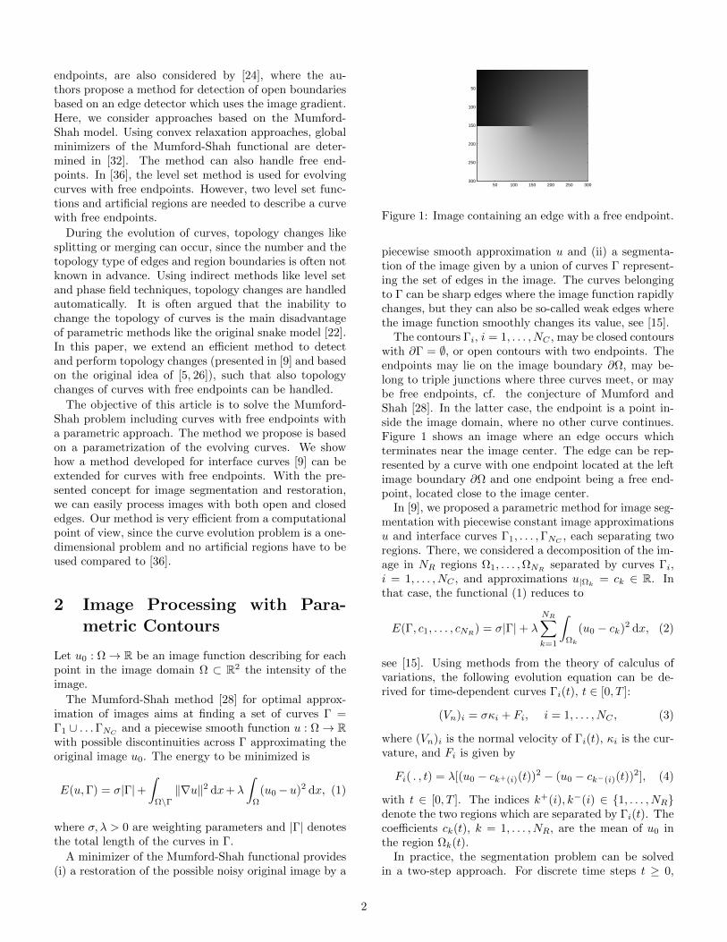
Figure 1: Image containing an edge with a free endpoint.
piecewise smooth approximation u and (ii) a segmenta-tion of the image given by a union of curves Γ represent-ing the set of edges in the image. The curves belongingto Γ can be sharp edges where the image function rapidlychanges, but they can also be so-called weak edges wherethe image function smoothly changes its value, see [15].
The contours Γi, i = 1, . . . , NC , may be closed contourswith ∂Γ = ∅, or open contours with two endpoints. Theendpoints may lie on the image boundary ∂Ω, may be-long to triple junctions where three curves meet, or maybe free endpoints, cf. the conjecture of Mumford andShah [28]. In the latter case, the endpoint is a point in-side the image domain, where no other curve continues.Figure 1 shows an image where an edge occurs whichterminates near the image center. The edge can be rep-resented by a curve with one endpoint located at the leftimage boundary ∂Ω and one endpoint being a free end-point, located close to the image center.
In [9], we proposed a parametric method for image seg-mentation with piecewise constant image approximationsu and interface curves Γ1, . . . ,ΓNC
, each separating tworegions. There, we considered a decomposition of the im-age in NR regions Ω1, . . . ,ΩNR
separated by curves Γi,i = 1, . . . , NC , and approximations u|Ωk
= ck ∈ R. Inthat case, the functional (1) reduces to
E(Γ, c1, . . . , cNR) = σ|Γ|+ λ
NR∑k=1
∫Ωk
(u0 − ck)2 dx, (2)
see [15]. Using methods from the theory of calculus ofvariations, the following evolution equation can be de-rived for time-dependent curves Γi(t), t ∈ [0, T ]:
(Vn)i = σκi + Fi, i = 1, . . . , NC , (3)
where (Vn)i is the normal velocity of Γi(t), κi is the cur-vature, and Fi is given by
Fi( . , t) = λ[(u0 − ck+(i)(t))2 − (u0 − ck−(i)(t))
2], (4)
with t ∈ [0, T ]. The indices k+(i), k−(i) ∈ 1, . . . , NRdenote the two regions which are separated by Γi(t). Thecoefficients ck(t), k = 1, . . . , NR, are the mean of u0 inthe region Ωk(t).
In practice, the segmentation problem can be solvedin a two-step approach. For discrete time steps t ≥ 0,
2
the coefficients ck are computed using the current setof curves. This is followed by an update of the curvesΓ(t) → Γ(t + ∆t), performed by solving the evolutionequation (3).
For some images, the piecewise constant approximationis not applicable, see the exemplary image in Figure 1.For such images, the image domain cannot be decom-posed in regions separated by interface curves.
Consequently, we modify the two-step approach of [9],such that also non-interface curves with free endpointscan be dealt with. In the first step, we will solve adiffusion equation in the image domain resulting in apiecewise smooth approximation u. Instead of using thecoefficients ck, we will consider for ~p ∈ Γi(t) the limitu±(~p) = limε→0,ε>0 u(~p ± ε~νi(~p)), where ~νi is a normalvector field on Γi(t). Having computed u, we solve theevolution equation (3) with a modified external term Fi,using u± instead of constants ck±(i).
Before, presenting further details, we first consider theregularity of a solution of the Mumford-Shah problemat the free endpoint. Fixing the curves Γ, let u denotethe minimizer of the Mumford-Shah energy (1). At freeendpoints, problems concerning the regularity of u occur,cf. [28]. Expressed in polar coordinates (r, φ) centered atthe free endpoint, the solution u is of the form
u(r, φ) = c r1/2 sin(1
2(φ− φ0)) + v(r, φ), (5)
where v is a C1-function and c, φ0 are constants, see [4].
For image segmentation, we later need to solve theproblem on a discrete set: Let Ωh be a rectangular gridof nodes covering Ω with grid size h > 0. We replace thesecond integral on the right hand side of (1) by a sumcontaining difference quotients of the form
∇ihu(~z) =1
h(u(~z + h~ei)− u(~z)), ~z ∈ Ωh, (6)
where ~ei ∈ R2 are the standard basis vectors of R2, i =1, 2. For image segmentation applications, we choose thepixel grid, i.e. we use h = 1. For the approximatingsum, we have to exclude terms where the line [~z, ~z + h~ei]intersects with the curve Γ.
Instead of the original Mumford-Shah functional (1),we thus consider the energy
Eh(Γ, u) = σ|Γ|+∑~z∈Ωh
s.t. ~z+h~e2∈Ωh
(1− αx(~z))(∇2hu(~z))2+
+∑~z∈Ωh
s.t. ~z+h~e1∈Ωh
(1− αy(~z))(∇1hu(~z))2 + λ
∫Ω
(u0 − u)2 dx,
(7)
where αx(~z), αy(~z) ∈ [0, 1] are scalar terms. If [~z, ~z+h~e1]intersects with Γ, αy(~z) is set to 1.
2.1 Example
We consider one single open curve Γ. Let ~x : [0, 1]→ R2
with ~x([0, 1]) = Γ be a parameterization of the curve.Let ~x(0) be a free endpoint and let ~x(1) intersect withthe image boundary.
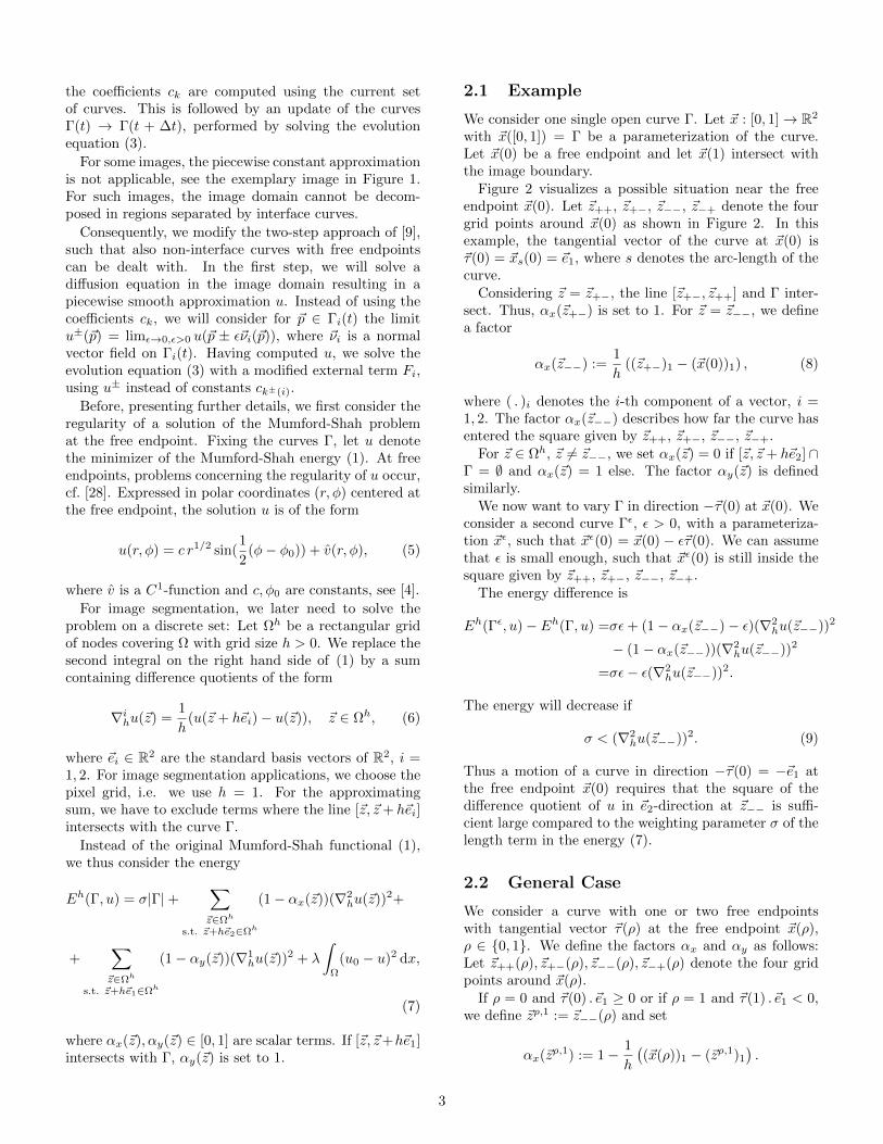
Figure 2 visualizes a possible situation near the freeendpoint ~x(0). Let ~z++, ~z+−, ~z−−, ~z−+ denote the fourgrid points around ~x(0) as shown in Figure 2. In thisexample, the tangential vector of the curve at ~x(0) is~τ(0) = ~xs(0) = ~e1, where s denotes the arc-length of thecurve.
Considering ~z = ~z+−, the line [~z+−, ~z++] and Γ inter-sect. Thus, αx(~z+−) is set to 1. For ~z = ~z−−, we definea factor
αx(~z−−) :=1
h((~z+−)1 − (~x(0))1) , (8)
where ( . )i denotes the i-th component of a vector, i =1, 2. The factor αx(~z−−) describes how far the curve hasentered the square given by ~z++, ~z+−, ~z−−, ~z−+.
For ~z ∈ Ωh, ~z 6= ~z−−, we set αx(~z) = 0 if [~z, ~z + h~e2] ∩Γ = ∅ and αx(~z) = 1 else. The factor αy(~z) is definedsimilarly.
We now want to vary Γ in direction −~τ(0) at ~x(0). Weconsider a second curve Γε, ε > 0, with a parameteriza-tion ~xε, such that ~xε(0) = ~x(0) − ε~τ(0). We can assumethat ε is small enough, such that ~xε(0) is still inside thesquare given by ~z++, ~z+−, ~z−−, ~z−+.
The energy difference is
Eh(Γε, u)− Eh(Γ, u) =σε+ (1− αx(~z−−)− ε)(∇2hu(~z−−))2
− (1− αx(~z−−))(∇2hu(~z−−))2
=σε− ε(∇2hu(~z−−))2.
The energy will decrease if
σ < (∇2hu(~z−−))2. (9)
Thus a motion of a curve in direction −~τ(0) = −~e1 atthe free endpoint ~x(0) requires that the square of thedifference quotient of u in ~e2-direction at ~z−− is suffi-cient large compared to the weighting parameter σ of thelength term in the energy (7).
2.2 General Case
We consider a curve with one or two free endpointswith tangential vector ~τ(ρ) at the free endpoint ~x(ρ),ρ ∈ 0, 1. We define the factors αx and αy as follows:Let ~z++(ρ), ~z+−(ρ), ~z−−(ρ), ~z−+(ρ) denote the four gridpoints around ~x(ρ).
If ρ = 0 and ~τ(0) . ~e1 ≥ 0 or if ρ = 1 and ~τ(1) . ~e1 < 0,we define ~zρ,1 := ~z−−(ρ) and set
αx(~zρ,1) := 1− 1
h
((~x(ρ))1 − (~zρ,1)1
).
3
Γ
~z++
~z+−~z−−
~z−+
~x(0)
αx(~z−−)
Figure 2: Illustration of the pixel grid close to the freeendpoint.
If ρ = 0 and ~τ(0) . ~e1 < 0 or if ρ = 1 and ~τ(1) . ~e1 ≥ 0,we define ~zρ,1 := ~z+−(ρ) and set
αx(~zρ,1) := 1− 1
h
((~zρ,1)1 − (~x(ρ))1
).
If ρ = 0 and ~τ(0) . ~e2 ≥ 0 or if ρ = 1 and ~τ(1) . ~e2 < 0,we define ~zρ,2 := ~z−−(ρ) and set
αy(~zρ,2) := 1− 1
h
((~x(ρ))2 − (~zρ,2)2
).
If ρ = 0 and ~τ(0) . ~e2 < 0 or if ρ = 1 and ~τ(1) . ~e2 ≥ 0,we define ~zρ,2 := ~z−+(ρ) and set
αy(~zρ,2) := 1− 1
h
((~zρ,2)2 − (~x(ρ))2
).
Using these definitions, we define the following factorsfor ~z ∈ Ωh:
αx(~z) =
1, if [~z, ~z + h~e2] ∩ Γ 6= ∅, and
~z 6= ~zρ,1, ρ ∈ 0, 1,αx(~zρ,1), if ~z = ~zρ,1, ρ ∈ 0, 1,0, else.
and
αy(~z) =
1, if [~z, ~z + h~e1] ∩ Γ 6= ∅, and
~z 6= ~zρ,2, ρ ∈ 0, 1,αy(~zρ,2), if ~z = ~zρ,2, ρ ∈ 0, 1,0, else.
For minimizing (7), we propose the following approach:
Assume the case of one curve Γ with two free endpointsparameterized by ~x : [0, 1]→ R2. In the first step, we fixu in (7) and consider for ~η : [0, 1] → R2 a variation of ~xof the form ~x+ ε~η, ε > 0.
Let Γε,η denote the image of ~x+ε~η. We use the notation
Eh(~η) := Eh(Γε,η, u) and compute
d
dε
∣∣∣∣ε=0
Eh(~η) =d
dε
∣∣∣∣ε=0
Eh(Γε,η, u)
=− σ∫
Γ
~xss . ~η ds−∫
Γ
F ~ν . ~η ds+
+ σ~xs(1) . ~η(1)− σ~xs(0) . ~η(0)
− sign(~τ(1) . ~e1)~η(1) . ~e1(∇2hu(~z1,1))2
− sign(~τ(1) . ~e2)~η(1) . ~e2(∇1hu(~z1,2))2
+ sign(~τ(0) . ~e1)~η(0) . ~e1(∇2hu(~z0,1))2
+ sign(~τ(0) . ~e2)~η(0) . ~e2(∇1hu(~z0,2))2.
For this computation, integration by parts and a trans-port theorem are applied. Further, ~ν is a normal vectorfield on Γ such that the pair (~xs, ~ν) is a positive orientedbasis of R2 and F is defined as the jump
F = λ[(u0 − u+)2 − (u0 − u−)2]. (10)
We define the following inner product for functions~η, ~χ : [0, 1]→ R2:
(~η, ~χ)2,Γ,∂Γ :=
∫Γ
~η . ~χ ds+ ~η(1) . ~χ(1) + ~η(0) . ~χ(0). (11)
Now, we consider a family of curves Γ(t), t ∈ [0, T ]. Let~x : [0, 1]× [0, T ]→ R2 be a mapping such that ~x( . , t) is aparameterization of Γ(t), t ∈ [0, T ]. We call ~x a solutionof the gradient flow equation, if
(~xt, ~η)2,Γ,∂Γ = − d
dε
∣∣∣∣ε=0
Eh(~η) (12)
holds for all ~η : [0, 1]→ R2.In the following, we consider particular choices of func-
tions ~η and derive evolution equations for the curve.First, we consider ~η = η0 ~ν for a scalar function η0 :[0, 1]→ R with η0(0) = η0(1) = 0. This provides∫
Γ(t)
~xt . ~ν η0 ds =
∫Γ(t)
(σ~xss . ~ν + F ) η0 ds.
Since η0 is arbitrary chosen (with value 0 at the end-points), we conclude the following equation for the nor-mal velocity of the curve:
Vn := ~xt . ~ν = σκ+ F, (13a)
using the identityκ~ν = ~xss. (13b)
Next, we choose ~η = η0~τ , where η0 : [0, 1] → R is ascalar function with η0(0) 6= 0 and η0(1) = 0, i.e. ~η(0) =~τ(0)η0(0) and ~η(1) = ~0. Inserting ~η in (12), and using(13a), (13b) and ~τ = ~xs, leads to
~xt(0) . ~τ(0)η0(0) = ση0(0)
− sign(~τ(0) . ~e1)~τ(0)η0(0) . ~e1(∇2hu(~z0,1))2+
− sign(~τ(0) . ~e2)~τ(0)η0(0) . ~e2(∇1hu(~z0,2))2.
4
Since η0(0) is arbitrary and sign(~τ(0) . ~ei)~τ(0) . ~ei =|~τ(0) . ~ei| for i = 1, 2, we conclude for the tangential ve-locity
Vtan(0) :=~xt(0) . ~τ(0)
=σ − |~τ(0) . ~e1|(∇2hu(~z0,1))2
− |~τ(0) . ~e2|(∇1hu(~z0,2))2. (13c)
Choosing η0(0) = 0 and η0(1) 6= 0, we can derive thefollowing equation for the tangential velocity in ~x(1):
Vtan(1) :=~xt(1) . ~τ(1)
=− σ + |~τ(1) . ~e1|(∇2hu(~z1,1))2
+ |~τ(1) . ~e2|(∇1hu(~z1,2))2. (13d)
Similarly, choosing ~η = η0~ν, provides the followingequations for the normal velocity at the free endpoints:
Vn(0) :=~xt(0) . ~ν(0)
=− sign(~τ(0) . ~e1)~ν(0) . ~e1(∇2hu(~z0,1))2
− sign(~τ(0) . ~e2)~ν(0) . ~e2(∇1hu(~z0,2))2, (13e)
Vn(1) :=~xt(0) . ~ν(0)
= + sign(~τ(1) . ~e1)~ν(1) . ~e1(∇2hu(~z1,1))2
+ sign(~τ(1) . ~e2)~ν(1) . ~e2(∇1hu(~z1,2))2. (13f)
The curve Γ will grow locally at ~x(0), if the curve movesin direction −~τ(0). In this case Vtan(0) = ~xt(0) . ~τ(0) < 0.Therefore,
σ < |~τ(0) . ~e1|(∇2hu(~z0,1))2+|~τ(0) . ~e2|(∇1
hu(~z0,2))|2 (14)
has to be satisfied such that the curve length increases.For the exemplary case ~τ(0) = ~e1, the condition reducesto (9), i.e. to the condition from the introductory exam-ple.
The curve Γ(t) will grow at ~x(1), if the curve movesin direction ~τ(1) leading to Vtan(1) > 0. Therefore, theinequality
σ < |~τ(1) . ~e1|(∇2hu(~z1,1))2 + |~τ(1) . ~e2|(∇1
hu(~z1,2))2 (15)
has to be satisfied.Since the term σ|Γ| in the energy (7) penalizes the
length of the curve, a curve can only grow in direction−~τ(0) or ~τ(1), if the derivative terms (∇ihu)2, i = 1, 2,are large compared to σ.
The scheme (13) describes the motion of the curve. ForNC curves Γ1, . . . ,ΓNC
, we can solve (13) for each curve.For a closed curve Γi, only the normal velocity (13a) withthe relation (13b) needs to be considered, on noting that~xi(0) = ~xi(1). In the case of triple junctions and intersec-tions with the image boundary, additional conditions forthe involved endpoints have to be considered. If triplejunctions occur, the evolution equations for the corre-sponding three curves which meet at the junction are
coupled. The cases with triple junctions and boundaryintersection points are described in [9] in detail.
We alternately solve the scheme of evolution equations(13) and recompute the approximating function u usingthe updated curve set. The function u is obtained bysolving a diffusion equation on Ωh. We note that (7) isformulated for a discrete set Ωh. We will describe in thenext section, how u is computed numerically.
3 Numerical Approximation
3.1 Numerical Solution of the EvolutionEquations
For computing the position of the evolving curves Γ nu-merically, we consider a decomposition of the interval[0, 1] of the form 0 = qi0 < qi1 < . . . < qiNi
= 1, fori = 1, . . . , NC . If Γi is a closed curve, we make use of theperiodicity Ni = 0, Ni + 1 = 1, −1 = Ni − 1, etc.
Further, let 0 = t0 < t1 < . . . < tM = T be apartitioning of the time interval [0, T ] with time steps∆tm := tm+1 − tm, m = 0, . . . ,M − 1. Smooth curvesΓi(tm), i = 1, . . . , NC , m = 0, . . . ,M are replaced by
polygonal curves Γmi given by nodes ~Xmi,j which are ap-
proximations of ~xi(qij , tm). Further, let κmi,j be an approx-
imation of κi(qij , tm). The derivative terms with respect
to time are replaced by difference quotients of the form
(~xi)t(qji , tm) ≈ 1
∆tm
(~Xm+1i,j − ~Xm
i,j
). (16)
Let hmi,j− 1
2
= ~Xmi,j − ~Xm
i,j−1, i = 1, . . . , NC , j = 1, . . . , Ni,
be the distance between two neighboring nodes. For eachcurve, we define a discete normal vector field ~νmi by
~νmi |[qij−1,qij ] := ~νmi,j− 1
2:=
( ~Xmi,j − ~Xm
i,j−1)⊥
hmi,j− 1
2
,
see also [6,7,9]. Here, ⊥ denotes the anti-clockwise rota-tion of a vector by π/2. Further, we define the following
weighted approximating normal vector at ~Xmi,j by
~ωmi,j :=hmi,j− 1
2
~νmi,j− 1
2
+ hmi,j+ 1
2
~νmi,j+ 1
2
hmi,j− 1
2
+ hmi,j+ 1
2
=( ~Xm
i,j+1 − ~Xmi,j−1)⊥
hmi,j− 1
2
+ hmi,j+ 1
2
,
for j = 1, . . . , Ni if ∂Γmi = ∅ and for j = 1, . . . , Ni − 1 if∂Γmi 6= ∅. In the latter case, we set
~ωmi,0 := ~νmi, 12=
( ~Xmi,1 − ~Xm
i,0)⊥
hmi, 12
,
~ωmi,Ni:= ~νmi,Ni− 1
2=
( ~Xmi,Ni− ~Xm
i,Ni−1)⊥
hmi,Ni− 1
2
.
5
The external term F is approximated by
Fmi,j :=λ[(u0( ~Xm
i,j)− u( ~Xmi,j + a~ωmi,j))
2
−(u0( ~Xmi,j)− u( ~Xm
i,j − a~ωmi,j))2],
with a small real number a > 0 if j is not the index of afree endpoint, and we set Fmi,j = 0 else.
The equation for the normal velocity (13a) is approxi-mated by
1
∆tm
(~Xm+1i,j − ~Xm
i,j
). ~ωmi,j = σκm+1
i,j + Fmi,j . (17a)
Thus, for computing Γm+1i , we use the previous curve Γmi
for the external term Fmi,j and for the weighted normal~ωmi,j .
For an approximation of (13b), we need to define anapproximation of (~xi)ss(q
ij , tm+1). For that, we make use
of difference quotients of the form
∆h,m2
~Xm+1i,j :=
2
hmi,j− 1
2
+ hmi,j+ 1
2
(( ~Xm+1
i,j+1 − ~Xm+1i,j )/hmi,j+ 1
2
−( ~Xm+1i,j − ~Xm+1
i,j−1)/hmi,j− 12
),
for i = 1, . . . , NC and j = 1, . . . , Ni, if ∂Γmi = ∅,and j = 1, . . . , Ni − 1, else. In case of equal spatialstep sizes hm
i,j− 12
= hmi,j+ 1
2
=: hmi , the term reduces to
( ~Xmi,j−1 − 2 ~Xm
i,j + ~Xmi,j+1)/((hmi )2), see also [9], where we
also defined and used these difference quotients.The equation (13b) is now approximated by
κm+1i,j ~ωmi,j = ∆h,m
2~Xm+1i,j , (17b)
for i = 1, . . . , NC , j = 1, . . . , Ni in case of closed curvesand j = 1, . . . , Ni − 1 in case of open curves.
In case of open curves, additional equations for theendpoints are needed. The case of triple junctions andboundary intersection points is described in [9]. Forcurves with free endpoints we introduce the tangentialvectors ~τmi,0 = ( ~Xm
i,1 − ~Xmi,0)/hi, 12 , and ~τmi,Ni
= ( ~Xmi,Ni−
~Xmi,Ni−1)/hi,Ni− 1
2. The equations (13c) and (13d) are ap-
proximated by
1
∆tm
(~Xm+1i,0 − ~Xm
i,0
). ~τmi,0 =
=σ − |~τmi,0 . ~e1|(∇2hu(~z0,1))2 − |~τmi,0 . ~e2|(∇1
hu(~z0,2))2,
(17c)
and
1
∆tm
(~Xm+1i,Ni
− ~Xmi,Ni
). ~τmi,Ni
=
=− σ + |~τmi,Ni. ~e1|(∇2
hu(~z1,1))2 + |~τmi,Ni. ~e2|(∇1
hu(~z1,2))2.
(17d)
Similarly, discrete versions of (13e) and (13f) can bestated using ~ωmi,0 and ~ωmi,Ni
as discrete normal vectors.
The scheme (17) is a numerical approximation of thescheme (13), where the parametric curves are replaced bypolygonal curves, and the smooth functions ~xi and κi arereplaced by continuous functions uniquely given by theirvalues at the nodes qij , i = 1, . . . , NC , j = 0, . . . , Ni.
The discrete scheme can be rewritten to a linear systemwith a sparse system matrix, similar as presented in [9],and can be solved with a fast direct solver like for examplethe UMFPACK algorithm [19].
3.2 Numerical Solution of the DenoisingProblem
For computing a numerical solution uh for the piece-wise smooth, denoised version u of u0, we consider forNx, Ny ∈ N the discrete set
Ωh := (ih, jh) : i = 0, . . . , Nx, j = 0 . . . , Ny ,
where Nx and Ny are the number of pixels in x- andy-direction. We define for i = 1, . . . , Nx, j = 1, . . . , Ny
Ax(i, j) =
h2, if [(i− 1)h, ih]× j ∩ Γmi0 = ∅,∀i0 ∈ 1, . . . , NC,
0, else,
Ay(i, j) =
h2, if i × [(j − 1)h, jh] ∩ Γmi0 = ∅,∀i0 ∈ 1, . . . , NC,
0, else.
Fixing the set of curves Γ, we consider the followingdiscrete energy:
Ediscr(uh) =
Nx∑i=1
Ny∑j=1
Ax(i, j)
(uhi,j − uhi−1,j
h
)2
+ Ay(i, j)
(uhi,j − uhi,j−1
h
)2
+ λ
Nx∑i=0
Ny∑j=0
h2(u0(ih, jh)− uhi,j
)2, (18)
which is a discrete analogue of∫Ω\Γ
(‖∇u‖2 dx+
∫Ωλ(u0 − u)2
)dx. Here uhi,j ap-
proximates u at the node (ih, jh). The piecewisecontinuous function uh is uniquely given by its value atthe points in Ωh.
By setting the terms Ax(i, j) or Ay(i, j) to zero atpoints where the line [(i − 1)h, jh), (ih, jh)] or [(ih, (j −1)h), (ih, jh)] intersects with one of the curves, we ap-proximate the integral over the set Ω \ Γ.
Taking the derivative of the right hand side of (18) withrespect to uhi,j and setting the resulting term to zero, leadsto a linear system. The corresponding system matrix is
6
sparse since each node (ih, jh) ∈ Ωh is only coupled toa few neighboring nodes. The resulting linear systemcan be solved with a fast direct or iterative solver byemploying the sparse matrix structure.
Considering h→ 0, we obtain in the limit ∇u . ~ν = 0 atthe curves belonging to Γ, and ∇u . ~n∂Ω = 0 at the imageboundary ∂Ω, where ~n∂Ω is a normal vector field at ∂Ω.For details, we refer to [9]. Consequently, we obtain anedge preserving image smoothing if Γ matches with theedges in the given image.
3.3 Topology Changes
During the evolution of curves, topology changes can oc-cur, since the edge set in the image and the boundariesof objects are not known in advance. Therefore, curvescan split into two or more subcurves, curves can mergeto one single curve, triple junctions and new curves mayoccur and curves can intersect with the image bound-ary such that new boundary nodes emerge. Further, acurve needs to be deleted if its length becomes too small.In [9], we extended the idea of [5, 26], and described amethod to detect topology changes of curves efficiently.The main idea is the use of an artificial background gridwhich covers the entire image domain Ω. We considersuccessively all nodes ~Xm
i,j and mark a grid element with
(i, j) if ~Xmi,j is the first node located in this array. If a
grid element is already marked with (i1, j1) and the nodes~Xmi,j and ~Xm
i1,j1are not neighbor nodes, a topology change
likely occurs close to this pair. Details on this methodfor curves without free endpoints are given in [9].
In principle, topology changes involving curves withfree endpoints can be detected similarly by using such abackground grid. In addition to the topology changeslisted above (splitting, merging, emergence of triplejunctions and boundary intersection points), topologychanges involving the free endpoints can occur: If two freeendpoints of one curve are located in one square of thebackground grid, an open contour becomes a closed con-tour. If two free endpoints of two different curves meet,the two curves merge to one single curve, and the formerfree endpoints become inner nodes of the new curve. If afree endpoint and an inner point of a curve meet, a triplejunction is created.
3.4 Summary of the Algorithm
We propose the following algorithm for image segmenta-tion and image restoration with parametric contours withpossible free endpoints:
Given a set of polygonal curves Γ0 = (Γ01, . . . ,Γ
0NC
)
and ~X0 = ( ~X01 , . . . ,
~X0NC
) with ~X0i ([0, 1]) = Γ0
i , performthe following steps for m = 0, 1, . . . ,M − 1:
1. Compute a denoised image approximation uh byminimizing (18) (solve the corresponding sparse lin-ear system).
2. Compute the external terms Fmi,j by using the solu-
tion uh of step 1. Compute ~Xm+1 by solving thelinear equation derived from the scheme (17).
3. Check whether topology changes occur. If so, exe-cute the topology change.
A segmentation of the image is given by the final set ofcurves ΓM . An image restoration is given by the imageapproximation uh from the time step tM .
3.5 Modifications
Step 2 of the algorithm above can additionally be splitin two sub-steps: First, we fix the free endpoints andwe let the inner nodes of the curve evolve. Then, we letthe endpoints evolve according to the above presenteddiscrete scheme.
The main effort of this method compared to the Chan-Vese method for interface curves is that we have to solvea two-dimensional diffusion equation (bulk equation) sev-eral times during the segmentation. In the experimentsdescribed in the next section, we perform 10 steps ofcurve evolution followed by a solution of the bulk equa-tion. Having computed uh, we use it for the next 10 curveevolution steps.
As an alternative, we can start the segmentation usinginterface curves and the image segmentation method de-scribed in [9] (based on the Chan-Vese method [15]) withpiecewise constant approximations. As a postprocessingstep, we can consider the derivatives of the image func-tion in normal direction at the final curves (or the jumpof the image function across the curves). We replace in-terface curves by curves with free endpoints if the deriva-tives in normal direction are locally very small. For that,we delete those parts of a curve where the derivative issmall which results in curves with free endpoints. Next,we compute some steps of the segmentation method withfree endpoints to obtain the final contours.
Topology changes occur only in rare cases when usinga postprocessing evolution of curves with free endpoints.In most situations, topology changes are already detectedin the previous evolution.
4 Results and Discussion
The method for image segmentation and restoration pre-sented in sections 2 and 3 are applied on some exem-plary test images. For all experiments presented in thissection, we use constant time steps sizes ∆tm = ∆t,m = 0, . . . ,M − 1.
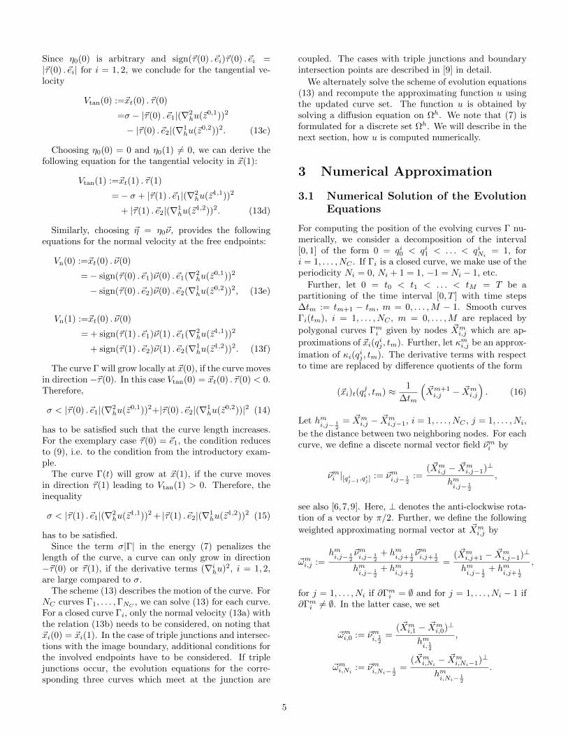
In the first experiment, we consider an example wherea contour with two free endpoints evolves in the imagedomain and detects an edge. Figure 3 presents the resultsof image segmentation and denoising. It can be observedthat the image is not smoothed out across the curve Γ.Further a growth of the curve in tangential direction can
7
50 100 150 200 250 300
50
100
150
200
250
30050 100 150 200 250 300
50
100
150
200
250
30050 100 150 200 250 300
50
100
150
200
250
300
50 100 150 200 250 300
50
100
150
200
250
30050 100 150 200 250 300
50
100
150
200
250
30050 100 150 200 250 300
50
100
150
200
250
300
Figure 3: Example image showing a contour with twofree endpoints. Original image and evolving contours (1strow) and denoised image (2nd row) for m = 1, 1000, 6000using ∆t = 0.032, σ = 2e− 5 and λ = 0.002.
be observed. The growth stops when the inequalities (14)and (15) become equalities. This depends on the absolutevalues of the difference quotients |∇ihu|, i = 1, 2, andthe weighting parameter σ. The image approximationu attends values in [0, 1]. In this image, differences ofthe form u(~x + h~ei) − u(~x) are typically of magnitude10−2. Since Ω = [1, 300] × [1, 300] and h = 1, |∇ihu|2 isof magnitude 10−4. Therefore, we have to choose a smallvalue for the weighting parameter σ, here, we choose σ =2e−5. If we used a normalized image domain Ω = [0, 1]×[0, 1], the pixel grid would have a grid size of h = 1/300and h2 = 1/90000. In this case, we would choose a weightσ of magnitude 1.
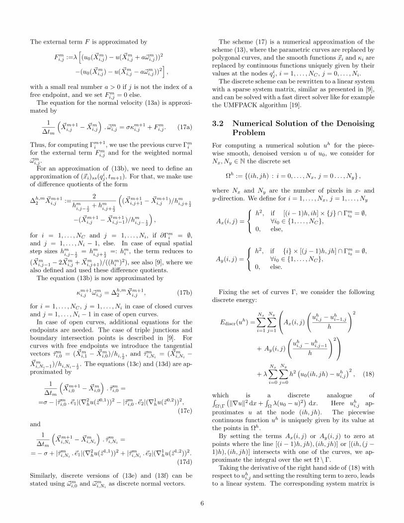
In a second experiment, we study a crack tip problemwhich has also been considered in [32]. The image func-tion is given by
u0(~x) = a√r(~x) sin(θ(~x)/2) + b, (19)
where r(~x) ≥ 0, θ(~x) ∈ (−π, π] are polar coordinates withr = 0 corresponding to the image center, and a, b ∈ R areconstants such that u0 attends values in [0, 1].
Figure 4 shows the evolution of a contour with onefree endpoint. The second endpoint belongs to the imageboundary. At time step m = 3000, the free endpoint islocated at the image center and the curve matches withthe edge in the image. As discussed above (see also Equa-tions (14) and (15)), the parameter σ, which weights thelength term, needs to be chosen small enough such thatthe curve can extend. If σ is fixed, the absolute value ofthe difference quotients must be large enough such thatthe length of the curve increases. In this example, theedge is a horizontal line and the position where the curvestops depends on the value of ∇2
hu, i.e. on the differencequotient in y-direction.
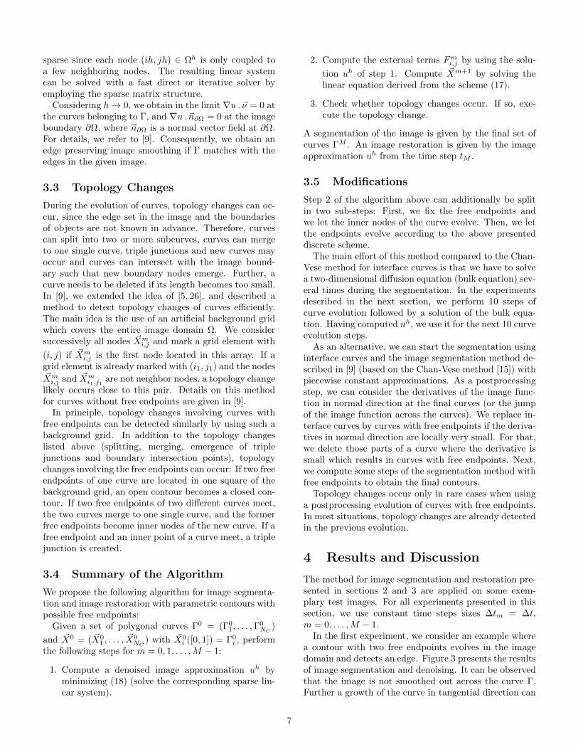
We rerun the example using σ = 0.002 and σ = 0.01instead of σ = 2e− 5. Figure 5 shows the results at time
50 100 150 200 250 300
50
100
150
200
250
30050 100 150 200 250 300
50
100
150
200
250
30050 100 150 200 250 300
50
100
150
200
250
300
Figure 4: Example image showing a contour with onefree endpoint and one boundary intersection point, seealso [32]. Evolving contours for m = 1, 500, 3000 using∆t = 0.001, σ = 2e− 5 and λ = 0.002.
50 100 150 200 250 300
50
100
150
200
250
30050 100 150 200 250 300
50
100
150
200
250
300
Figure 5: Dependency on the weighting parameter usingσ = 0.002 (left) and σ = 0.01 (right), ∆t = 0.001 andλ = 0.002 for m = 3000. If a too large weight is chosenfor the length term in (7), the curve does not reach theimage center.
step m = 3000. In both cases, the free endpoint doesnot reach the center of the image since the value of σ hasbeen set larger. The growth of the curve already stopsat larger values of ∇2
hu, recall conditions (14) and (15)).We even let the curve evolve until time step m = 5000,but we observed no significant motion between m = 3000and m = 5000.
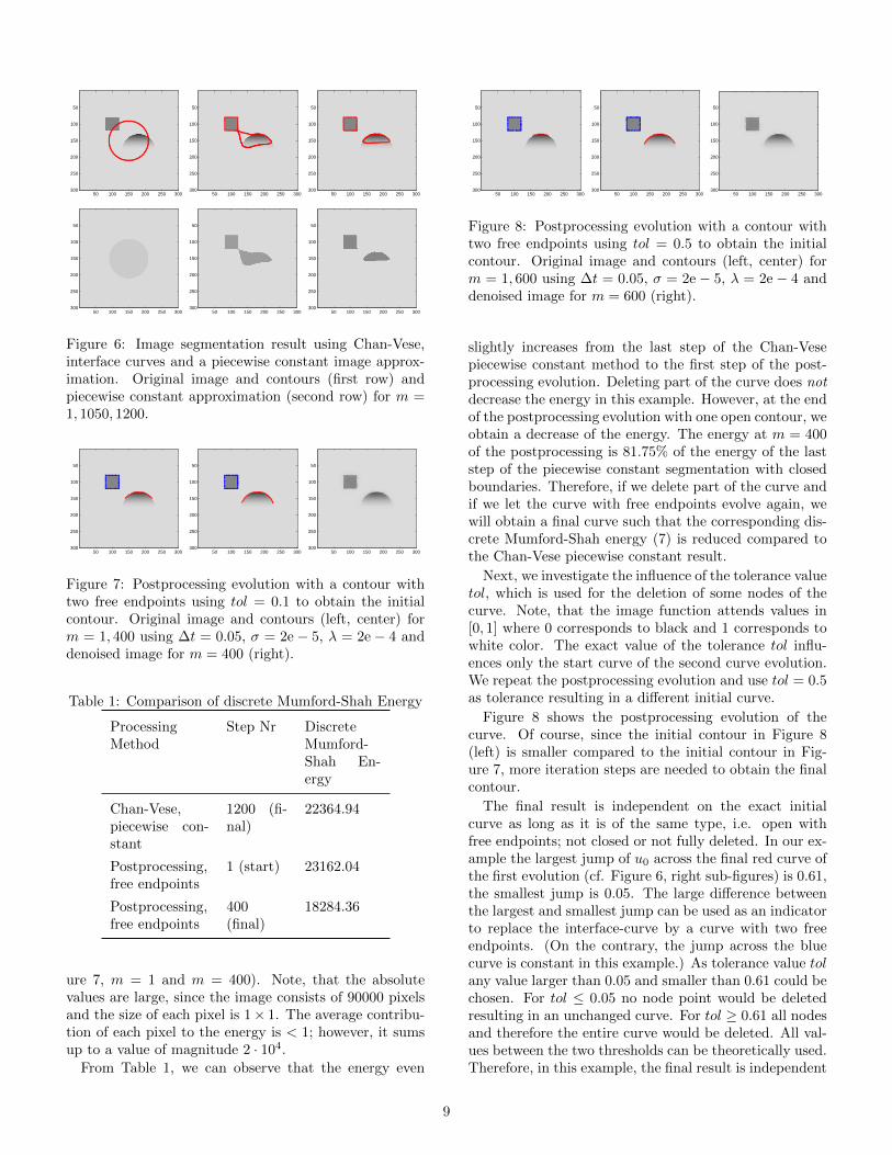
In another experiment, which demonstrates the evo-lution of curves with free endpoints, we first apply theparametric method of [9] to the Chan-Vese problem [15]using interface-curves. This means, that we first seg-ment a given image in regions separated by interfacecurves, see Figure 6. We start with one large initial curvewhich splits up in two sub-curves. This example thus alsodemonstrates the handling of a topology change.
In a postprocessing step, we delete those nodes wherethe jump of u0 across the curve is smaller than a giventolerance of tol = 0.1. This results in one closed curve,where no points are deleted (blue curve in Figure 7), andin one curve with two free endpoints (red curve). Fig-ure 7 shows the results of a postprocessing evolution ofthe curve. This example shows that our methods for im-age segmentation and denoising can be applied also onimages with both open and closed edges.
Table 1 shows the values of the discrete Mumford-Shahenergy (7) for the last step of the Chan-Vese piecewiseconstant segmentation with closed region boundaries (cf.Figure 6, m = 1200) and for the initial and final stepof the postprocessing with one open boundary (cp. Fig-
8
50 100 150 200 250 300
50
100
150
200
250
30050 100 150 200 250 300
50
100
150
200
250
30050 100 150 200 250 300
50
100
150
200
250
300
50 100 150 200 250 300
50
100
150
200
250
30050 100 150 200 250 300
50
100
150
200
250
30050 100 150 200 250 300
50
100
150
200
250
300
Figure 6: Image segmentation result using Chan-Vese,interface curves and a piecewise constant image approx-imation. Original image and contours (first row) andpiecewise constant approximation (second row) for m =1, 1050, 1200.
50 100 150 200 250 300
50
100
150
200
250
30050 100 150 200 250 300
50
100
150
200
250
30050 100 150 200 250 300
50
100
150
200
250
300
Figure 7: Postprocessing evolution with a contour withtwo free endpoints using tol = 0.1 to obtain the initialcontour. Original image and contours (left, center) form = 1, 400 using ∆t = 0.05, σ = 2e − 5, λ = 2e − 4 anddenoised image for m = 400 (right).
Table 1: Comparison of discrete Mumford-Shah Energy
ProcessingMethod
Step Nr DiscreteMumford-Shah En-ergy
Chan-Vese,piecewise con-stant
1200 (fi-nal)
22364.94
Postprocessing,free endpoints
1 (start) 23162.04
Postprocessing,free endpoints
400(final)
18284.36
ure 7, m = 1 and m = 400). Note, that the absolutevalues are large, since the image consists of 90000 pixelsand the size of each pixel is 1× 1. The average contribu-tion of each pixel to the energy is < 1; however, it sumsup to a value of magnitude 2 · 104.
From Table 1, we can observe that the energy even
50 100 150 200 250 300
50
100
150
200
250
30050 100 150 200 250 300
50
100
150
200
250
30050 100 150 200 250 300
50
100
150
200
250
300
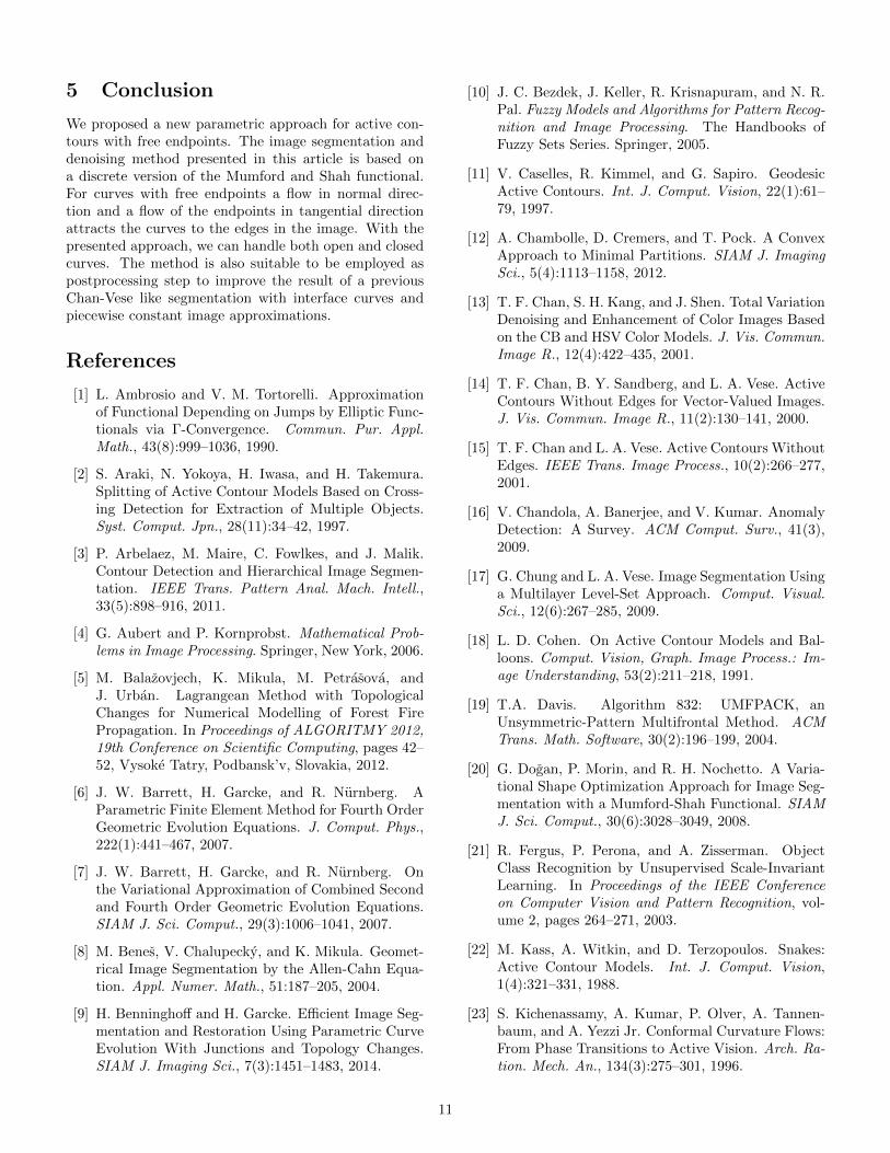
Figure 8: Postprocessing evolution with a contour withtwo free endpoints using tol = 0.5 to obtain the initialcontour. Original image and contours (left, center) form = 1, 600 using ∆t = 0.05, σ = 2e − 5, λ = 2e − 4 anddenoised image for m = 600 (right).
slightly increases from the last step of the Chan-Vesepiecewise constant method to the first step of the post-processing evolution. Deleting part of the curve does notdecrease the energy in this example. However, at the endof the postprocessing evolution with one open contour, weobtain a decrease of the energy. The energy at m = 400of the postprocessing is 81.75% of the energy of the laststep of the piecewise constant segmentation with closedboundaries. Therefore, if we delete part of the curve andif we let the curve with free endpoints evolve again, wewill obtain a final curve such that the corresponding dis-crete Mumford-Shah energy (7) is reduced compared tothe Chan-Vese piecewise constant result.
Next, we investigate the influence of the tolerance valuetol, which is used for the deletion of some nodes of thecurve. Note, that the image function attends values in[0, 1] where 0 corresponds to black and 1 corresponds towhite color. The exact value of the tolerance tol influ-ences only the start curve of the second curve evolution.We repeat the postprocessing evolution and use tol = 0.5as tolerance resulting in a different initial curve.
Figure 8 shows the postprocessing evolution of thecurve. Of course, since the initial contour in Figure 8(left) is smaller compared to the initial contour in Fig-ure 7, more iteration steps are needed to obtain the finalcontour.
The final result is independent on the exact initialcurve as long as it is of the same type, i.e. open withfree endpoints; not closed or not fully deleted. In our ex-ample the largest jump of u0 across the final red curve ofthe first evolution (cf. Figure 6, right sub-figures) is 0.61,the smallest jump is 0.05. The large difference betweenthe largest and smallest jump can be used as an indicatorto replace the interface-curve by a curve with two freeendpoints. (On the contrary, the jump across the bluecurve is constant in this example.) As tolerance value tolany value larger than 0.05 and smaller than 0.61 could bechosen. For tol ≤ 0.05 no node point would be deletedresulting in an unchanged curve. For tol ≥ 0.61 all nodesand therefore the entire curve would be deleted. All val-ues between the two thresholds can be theoretically used.Therefore, in this example, the final result is independent
9

20 40 60
10
20
30
40
50
60
70
80
90
10020 40 60
10
20
30
40
50
60
70
80
90
10020 40 60
10
20
30
40
50
60
70
80
90
10020 40 60
10
20
30
40
50
60
70
80
90
100
Figure 9: Medical image segmentation using Chan-Vese,interface curves and a piecewise constant image ap-proximation. Original image and contours for m =1, 400, 1000, 2500. Image courtesy: Dr. Declan O’Reganand the Robert Steiner MR Unit, MRC Clinical SciencesCentre, Imperial College London.
20 40 60
10
20
30
40
50
60
70
80
90
10020 40 60
10
20
30
40
50
60
70
80
90
10020 40 60
10
20
30
40
50
60
70
80
90
10020 40 60
10
20
30
40
50
60
70
80
90
100
Figure 10: Postprocessing segmentation with free end-points. Original image and contours (far left, left, right)for m = 1, 100, 500 using ∆t = 0.008, σ = 3.3e − 5,λ = 0.0167 and denoised image (far right) for m = 500.Image courtesy: Dr. Declan O’Regan and the RobertSteiner MR Unit, MRC Clinical Sciences Centre, Impe-rial College London.
on the exact value of tol as long it is in (0.05, 0.61).
Next, we demonstrate an example where a real, med-ical image is processed. Figure 9 and Figure 10 showan excerpt of a medical image and the result of an edgedetection. We first use the Chan-Vese algorithm withpiecewise constant image approximation for segmentingthe image, see Figure 9. In this first segmentation step,also topology changes occur. The initial closed curvetouches twice the image boundary and splits up in twoopen curves each with two boundary intersection points.After the preceding segmentation, a part of the red curveis deleted (using a tolerance of 0.1 for the jump across thecurve) resulting in a curve with free endpoints. Figure 10shows the result of the postprocessing evolution. Smalltangential motions of the free endpoints can be observed.
Finally, we study an example where several topologychanges occur. Figure 11 shows an example where westart with many small initial curves. A similar image isalso considered in [32]. Many of the small initial linesshrink and are deleted when their curve length becomestoo small. Additonal topology changes occur: Near theupper left corner of the image, two curves merge at theirfree endpoints to one curve. Further, three free endpointsbecome boundary intersection points, and a triple junc-tion emerges when a free endpoint meets another curve
50 100 150 200 250 300
50
100
150
200
250
30050 100 150 200 250 300
50
100
150
200
250
30050 100 150 200 250 300
50
100
150
200
250
300
50 100 150 200 250 300
50
100
150
200
250
30050 100 150 200 250 300
50
100
150
200
250
30050 100 150 200 250 300
50
100
150
200
250
300
Figure 11: Image segmentation and contour detectionwith topology changes. The final segmentation containstwo free endpoints, one triple junctions and three bound-ary intersection points. Original image and contours form = 1, 100, 250, 400, 750, 1200 using ∆t = 1, σ = 1e − 4,λ = 1e− 3.
at an inner node. The topology changes are detected asdescribed in Section 3.3 and [9].
An advantage of the parametric method is that wecan easily handle non-interface curves and complex curvenetworks including triple junctions. The curve evolutionscheme is very similar to the scheme presented in [9] forinterface-curves. Instead of computing the mean value ofthe image function in regions, we have to solve a diffusionbulk equation. Additional to the motion of the curve innormal direction, free endpoints can move in tangentialdirection.
There are alternatives to parametric methods to de-scribe an evolving curve. The level set method [30] is verypopular for image processing applications and in partic-ular for active contours methods, see e.g. [25], [11], [23],[15], [37], [35] to mention a few. In level set methods, ahypersurface is embedded as the zero level set of a func-tion defined on the image domain Ω. With level set tech-niques, free endpoints however cannot be handled withone single level set function: Since level set methods em-bed a curve as zero level set of a function Φ : Ω→ R, thecurve is an interface between two regions Φ > 0 andΦ < 0. Therefore level sets are always closed or meetthe image boundary at their endpoints. Non-interfacecurves can be handled by using two level set functions Φand Ψ and by using artificial regions, see [36]. A curvewith free endpoints can then be represented by the inter-face between the artificial regions Φ > 0∩Ψ > 0 andΦ > 0 ∩ Ψ < 0, for example.
Using our direct, parametric approach it is not neces-sary to introduce artificial regions. Further our methodis very efficient, since the curve evolution is only a one-dimensional problem.
10
5 Conclusion
We proposed a new parametric approach for active con-tours with free endpoints. The image segmentation anddenoising method presented in this article is based ona discrete version of the Mumford and Shah functional.For curves with free endpoints a flow in normal direc-tion and a flow of the endpoints in tangential directionattracts the curves to the edges in the image. With thepresented approach, we can handle both open and closedcurves. The method is also suitable to be employed aspostprocessing step to improve the result of a previousChan-Vese like segmentation with interface curves andpiecewise constant image approximations.
References
[1] L. Ambrosio and V. M. Tortorelli. Approximationof Functional Depending on Jumps by Elliptic Func-tionals via Γ-Convergence. Commun. Pur. Appl.Math., 43(8):999–1036, 1990.
[2] S. Araki, N. Yokoya, H. Iwasa, and H. Takemura.Splitting of Active Contour Models Based on Cross-ing Detection for Extraction of Multiple Objects.Syst. Comput. Jpn., 28(11):34–42, 1997.
[3] P. Arbelaez, M. Maire, C. Fowlkes, and J. Malik.Contour Detection and Hierarchical Image Segmen-tation. IEEE Trans. Pattern Anal. Mach. Intell.,33(5):898–916, 2011.
[4] G. Aubert and P. Kornprobst. Mathematical Prob-lems in Image Processing. Springer, New York, 2006.
[5] M. Balazovjech, K. Mikula, M. Petrasova, andJ. Urban. Lagrangean Method with TopologicalChanges for Numerical Modelling of Forest FirePropagation. In Proceedings of ALGORITMY 2012,19th Conference on Scientific Computing, pages 42–52, Vysoke Tatry, Podbansk’v, Slovakia, 2012.
[6] J. W. Barrett, H. Garcke, and R. Nurnberg. AParametric Finite Element Method for Fourth OrderGeometric Evolution Equations. J. Comput. Phys.,222(1):441–467, 2007.
[7] J. W. Barrett, H. Garcke, and R. Nurnberg. Onthe Variational Approximation of Combined Secondand Fourth Order Geometric Evolution Equations.SIAM J. Sci. Comput., 29(3):1006–1041, 2007.
[8] M. Benes, V. Chalupecky, and K. Mikula. Geomet-rical Image Segmentation by the Allen-Cahn Equa-tion. Appl. Numer. Math., 51:187–205, 2004.
[9] H. Benninghoff and H. Garcke. Efficient Image Seg-mentation and Restoration Using Parametric CurveEvolution With Junctions and Topology Changes.SIAM J. Imaging Sci., 7(3):1451–1483, 2014.
[10] J. C. Bezdek, J. Keller, R. Krisnapuram, and N. R.Pal. Fuzzy Models and Algorithms for Pattern Recog-nition and Image Processing. The Handbooks ofFuzzy Sets Series. Springer, 2005.
[11] V. Caselles, R. Kimmel, and G. Sapiro. GeodesicActive Contours. Int. J. Comput. Vision, 22(1):61–79, 1997.
[12] A. Chambolle, D. Cremers, and T. Pock. A ConvexApproach to Minimal Partitions. SIAM J. ImagingSci., 5(4):1113–1158, 2012.
[13] T. F. Chan, S. H. Kang, and J. Shen. Total VariationDenoising and Enhancement of Color Images Basedon the CB and HSV Color Models. J. Vis. Commun.Image R., 12(4):422–435, 2001.
[14] T. F. Chan, B. Y. Sandberg, and L. A. Vese. ActiveContours Without Edges for Vector-Valued Images.J. Vis. Commun. Image R., 11(2):130–141, 2000.
[15] T. F. Chan and L. A. Vese. Active Contours WithoutEdges. IEEE Trans. Image Process., 10(2):266–277,2001.
[16] V. Chandola, A. Banerjee, and V. Kumar. AnomalyDetection: A Survey. ACM Comput. Surv., 41(3),2009.
[17] G. Chung and L. A. Vese. Image Segmentation Usinga Multilayer Level-Set Approach. Comput. Visual.Sci., 12(6):267–285, 2009.
[18] L. D. Cohen. On Active Contour Models and Bal-loons. Comput. Vision, Graph. Image Process.: Im-age Understanding, 53(2):211–218, 1991.
[19] T.A. Davis. Algorithm 832: UMFPACK, anUnsymmetric-Pattern Multifrontal Method. ACMTrans. Math. Software, 30(2):196–199, 2004.
[20] G. Dogan, P. Morin, and R. H. Nochetto. A Varia-tional Shape Optimization Approach for Image Seg-mentation with a Mumford-Shah Functional. SIAMJ. Sci. Comput., 30(6):3028–3049, 2008.
[21] R. Fergus, P. Perona, and A. Zisserman. ObjectClass Recognition by Unsupervised Scale-InvariantLearning. In Proceedings of the IEEE Conferenceon Computer Vision and Pattern Recognition, vol-ume 2, pages 264–271, 2003.
[22] M. Kass, A. Witkin, and D. Terzopoulos. Snakes:Active Contour Models. Int. J. Comput. Vision,1(4):321–331, 1988.
[23] S. Kichenassamy, A. Kumar, P. Olver, A. Tannen-baum, and A. Yezzi Jr. Conformal Curvature Flows:From Phase Transitions to Active Vision. Arch. Ra-tion. Mech. An., 134(3):275–301, 1996.
11
[24] R. Kimmel and A. M. Bruckstein. RegularizedLaplacian Zero Crossings as Optimal Edge Integra-tors. Int. J. Comput. Vision, 53(3):225–243, 2003.
[25] R. Malladi, J. A. Sethian, and B. C. Vemuri. ShapeModeling with Front Propagation: A Level Set Ap-proach. IEEE Trans. Pattern Anal. Mach. Intell.,17(2):158–175, 1995.
[26] K. Mikula and J. Urban. New Fast and Stable La-grangean Method for Image Segmentation. In Pro-ceedings of the 5th International Congress on Imageand Signal Processing (CISP 2012), pages 834–842,Chongquing, China, 2012.
[27] J. Mille. Narrow Band Region-Based Active Con-tours and Surfaces for 2D and 3D Segmentation.Comput. Vis. Image Und., 113(9):946–965, 2009.
[28] D. Mumford and J. Shah. Optimal Approxima-tion by Piecewise Smooth Functions and AssociatedVariational Problems. Commun. Pur. Appl. Math.,42:577–685, 1989.
[29] M. S. Nixon and A. S. Aguado. Feature Extractionand Image Processing. Newnes, Oxford, Auckland,Boston, Johannesburg, Melbourne, New Delhi, 1stedition, 2002.
[30] S. Osher and J. A. Sethian. Fronts Propagating withCurvature Dependent Speed: Algorithms Based onHamilton-Jacobi Formulations. J. Comput. Phys.,79(1):12–49, 1988.
[31] N. Paragios and R. Deriche. Geodesic Active Con-tours and Level Sets for Detection and Tracking ofMoving Objects. IEEE Trans. Pattern Anal. Mach.Intell., 22(3):266–280, 2000.
[32] T. Pock, D. Cremers, H. Bischof, and A. Chambolle.An Algorithm for Minimizing the Mumford-ShahFunctional. In Proceedings of the 12th IEEE In-ternational Conference on Computer Vision (ICCV2009), pages 1133–1140, 2009.
[33] R. Ronfard. Region-Based Strategies for Active Con-tour Models. Int. J. Comput. Vision, 13(2):229–251,1994.
[34] L. I. Rudin, S. Osher, and E. Fatemi. NonlinearTotal Variation Based Noise Removal Algorithms.Physica D, 60(1-4):259–268, 1992.
[35] G. Sapiro. Geometric Partial Differential Equationsand Image Analysis. Cambridge University Press,New York, 2006.
[36] H. Schaeffer and L. Vese. Active Contours withFree Endpoints. J. Math. Imaging Vis., 49(1):20–36, 2014.
[37] A. Tsai, A. Yezzi, and A. S. Willsky. Curve Evo-lution Implementation of the Mumford-Shah Func-tional for Image Segmentation, Denoising, Interpo-lation and Magnification. IEEE Trans. Image Pro-cess., 10(8):1169–1186, 2001.
[38] Z. Yu and C. Bajaj. Anisotropic Vector Diffusionin Image Smoothing. In Proceedings of Interna-tional Conference on Image Processing, pages 828–831, 2002.
12