image compression with a hierarchical neural · pdf fileimage compression with a hierarchical...

International Journal of Computer and Engineering Management

Image Compression with a Hierarchical Neural Network

By. Aran Namphol, Steven H. Chin, Mohammed Arozullah Catholic University of America This paper is published with permission. It was first published in "IEEE TRANSACTIONS ON AEROSPACE AND ELECTRONIC SYSTEMS" January, 1996 Volume 32 Number 1, pp 326 - 338

1.Nomenclature 2.Introduction 3.Hierarchical Neural Network Architecture 4.Analytical Results 5.Simulation Results 6.Conclusions 7.References 8.About the Authors

A neural network data compression method is presented. This network accepts a large amount of image or text data, compresses it for storage or transmission, and subsequently restores it when desired. A new training method, referred to as the Nested Training Algorithm (NTA), that reduces the training time considerably is presented. Analytical results are provided for the specification of the optimal learning rates and the size of the training data for a given image of specified dimensions. Performance of the network has been evaluated using both synthetic and real-world data. It is shown that the developed architecture and training algorithm provide high compression ratio and low distortion while maintaining the ability to generalize, and is very robust as well.

1. NOMENCLATURE

N Number of pixels in one dimension of the scene

Nh Number of hidden nodes in outer loop neural network

CR Compression ratio

p Size of pixel patch in one dimension

Q Number of hidden nodes in inner loop neural network

M Number of subscenes

T Number of pixel patches in one subscene

S Entire scene

S[m] mth subscene tth pixel patch of mth subscene

file:///C|/Documents%20and%20Settings/Ponn/Desktop/ijcim/past_editions/1997V05N1/doc1.htm (1 of 23)25/8/2549 10:39:49


Output of hidden layer for tth pixel patch, rth node of mth subscene for outer loop neural networks

Weight from kth node of input layer to rth node of hidden layer for outer loop neural networks

kth reproduced pixel value corresponding to tth p * p pixel patch of mth subscene

Weight from rth node of hidden layer to kth node of output layer for outer loop neural networks

Htraining data for inner loop neural networks from hidden layer output of outer loop neural networks

H[t] tth training pattern of H

Cq Output of qth compressor layer node

Weight connection between jth node of combiner layer and qth node of compressor layer of inner loop neural networks

Dj Output of jth decombiner layer node

Weight connection between qth node of compressor layer and jth node of decombiner layer of inner loop neural networks

R Correlation matrix

Nx Number of nodes of input layer for two-layer network

Ny Number of nodes of output layer for two-layer network

Nw Number of weight in two-layer network

Np Number of patterns in training set for two-layer network

K Ratio of number of hidden nodes to input nodes º 1/CR

G Generalization constant

C Network capacity constant

Cu Upper bound on network capacity

x(i,j) Pixel intensity at spatial coordinates (i, j)

w(i,j)Two-dimensional sequence of independent and identically distributed, zero-mean Gaussian random variables with common variance .

II. INTRODUCTION

There has been a considerable amount of activity in the area of data compression during the last twenty years [1,2]. Traditional data compression techniques have included transform-oriented methods and vector quantization. Transform-based compression techniques project the data onto a domain which requires fewer coefficients for good data representation. The performance of transform-based data compression systems (e g, JPEG and MPEG) is highly dependent on the type of transform being used (e g, cosine transform, wavelet transform). Vector and adaptive-vector quantization techniques require the development of an appropriate code book to compress the data. The performance of a vector quantizer compression system is highly dependent on the quality of the code book, and operational times can be long if the code book is large. There have been more recent developments in data compression based on the study of the brain mechanism for vision and scene analysis [3]. These techniques have achieved a very large compression ratio (on the order of 100 : l),



but can require extensive processing to extract the relevant features.

Neural networks offer the potential for providing a novel solution to the problem of data compression by its ability to generate an internal data representation. Ackley used Boltzman's Machine to perform data encoding and decoding [4]. Rummelhart indicated the potential of neural networks to achieve data encoding/decoding [5]. Cottrell employed a two-layer neural network using the standard back propagation training algorithm to obtain image compression [6, 7]. In Cottrell's method, an image (or scene) is divided into a number of nonoverlapping pixel patches. These pixel patches are later used to train the network. Actual compression of the whole scene is then carried out by using this trained network to compress the nonoverlapping pixel patches one by one, and then combining the corresponding output into the compressed scene. Compared with vector quantization, Cottlell's method has several advantages such as shorter encoding/decoding time, and no explicit utilization of codebooks. However, Cottrell's method exploited only the correlation between pixels within each of the training patches. Therefore, only limited amount of compression could be achieved.

III. HIERARCHICAL NEURAL NETWORK ARCHITECTURE

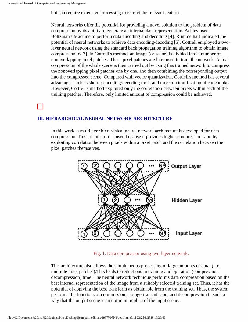
In this work, a multilayer hierarchical neural network architecture is developed for data compression. This architecture is used because it provides higher compression ratio by exploiting correlation between pixels within a pixel patch and the correlation between the pixel patches themselves.

Fig. 1. Data compressor using two-layer network.

This architecture also allows the simultaneous processing of large amounts of data, (i .e., multiple pixel patches).This leads to reductions in training and operation (compression-decompression) time. The neural network technique performs data compression based on the best internal representation of the image from a suitably selected training set. Thus, it has the potential of applying the best transform as obtainable from the training set. Thus, the system performs the functions of compression, storage-transmission, and decompression in such a way that the output scene is an optimum replica of the input scene.



A. Network Design Approach

The images to be compressed consist of a 2-dimensional square N * N array of pixels. The discussion easily generalizes for images which are not square. Hypothetically, one network trained by the backpropagation algorithm [8], consisting of N2 nodes at the input and output layers and Nh nodes at the hidden layer is sufficient to achieve data compression. The compression ratio (CR) for this network is given by

(1)

This is depicted in Fig. 1. A drawback of this method is that for large N, the training time is prohibitively long and the physical resources required to build such a large network may not be easily available.

Instead of using the whole image as the training set, the image can be partitioned into p * p pixel patches, where p < N. These pixel patches are subsequently used as training patterns for the training set. The resulting network architecture is identical to that of Fig 1, except that those are p2 nodes at the input and output layers. The resulting CR is

(2)

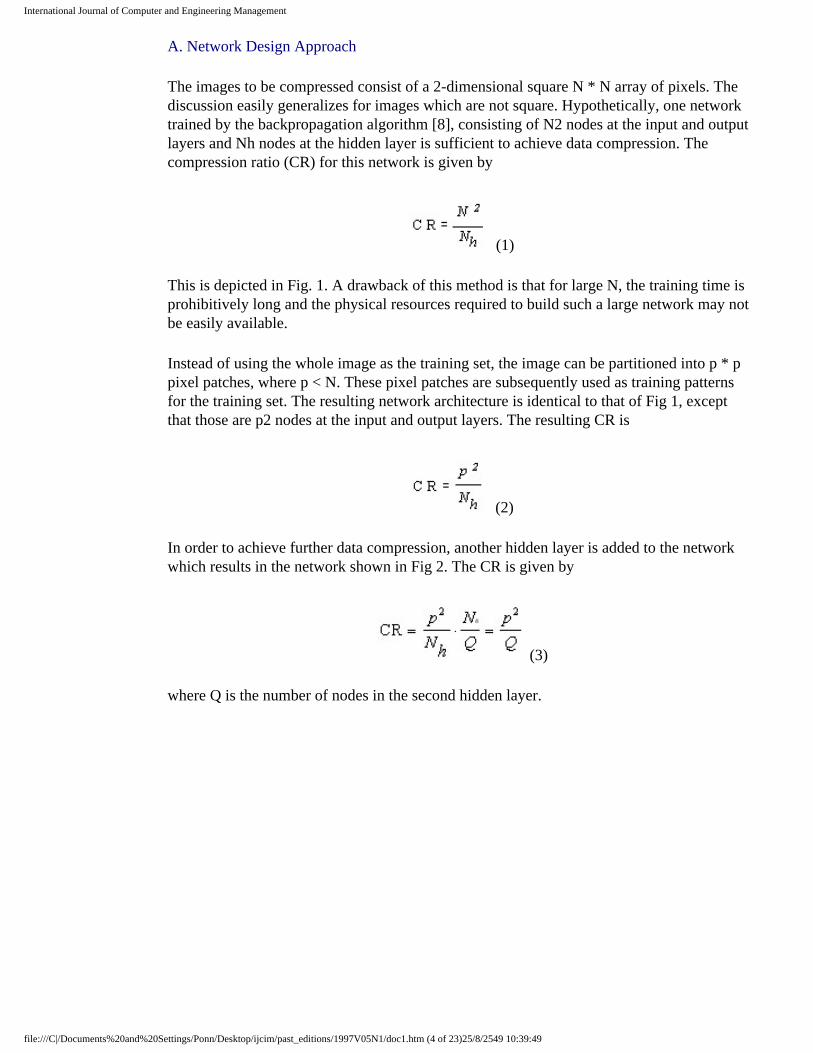
In order to achieve further data compression, another hidden layer is added to the network which results in the network shown in Fig 2. The CR is given by

(3)

where Q is the number of nodes in the second hidden layer.



Fig 2. Multilayer architecture for high order data compression-decompressions

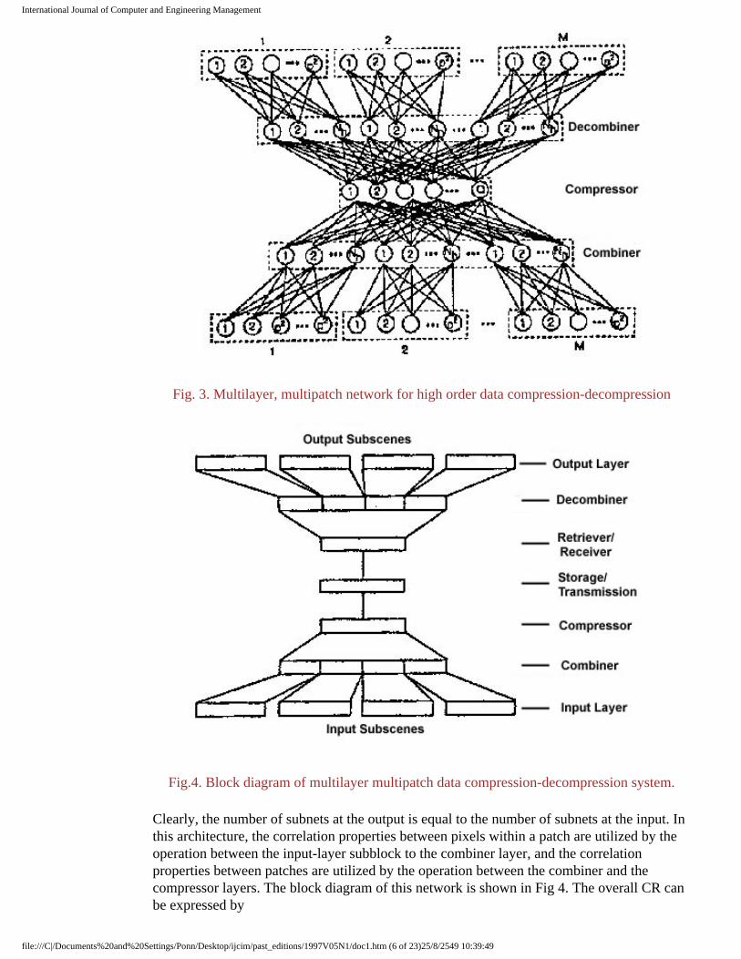
As a final step, a four-layer architecture for high order data compression using multiple p * p pixel patches as input as shown in Fig 3 is considered. It is a symmetric four-layer neural network. The development of this neural network begins by dividing the input image (scene) into M disjoint subscenes. Each subscene is further partitioned into a number of p*p-dimensional pixel patches. These pixel patches are later used as the training patterns for the subnetworks. The overall network consists of three sections: input-layer, hidden-layer, and output-layer sections. The input-layer section is comprised of M blocks, where each block has p2 nodes. The hidden-layer section consists of three layers: combiner, compressors and decombiner layers. The combiner layer acts as the multiplexer to the input subblocks. The number of nodes in the combiner is less than that in the input layer. The compressor further compresses the output of the combiner and produces the internal representation of the scene. The output of the compressor is then stored as the compressed image .To reconstruct the image, the stored values must be decombined. The decombiner acts as the demultiplexer, where its output is divided into subblocks. The number of subblocks is equal to the number of the input subnetworks. Each of the subblocks is applied to a subnetwork which produces the corresponding output subscene.



Fig. 3. Multilayer, multipatch network for high order data compression-decompression

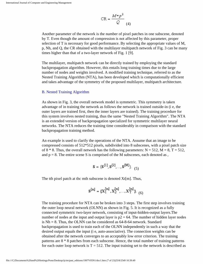
Fig.4. Block diagram of multilayer multipatch data compression-decompression system.

Clearly, the number of subnets at the output is equal to the number of subnets at the input. In this architecture, the correlation properties between pixels within a patch are utilized by the operation between the input-layer subblock to the combiner layer, and the correlation properties between patches are utilized by the operation between the combiner and the compressor layers. The block diagram of this network is shown in Fig 4. The overall CR can be expressed by



(4)

Another parameter of the network is the number of pixel patches in one subscene, denoted by T. Even though the amount of compression is not affected by this parameter, proper selection of T is necessary for good performance. By selecting the appropriate values of M, p, Nh, and Q, the CR obtained with the multilayer multipatch network of Fig. 3 can be many times higher than that of a two-layer network of Fig. 1 [9].

The multilayer, multipatch network can be directly trained by employing the standard backpropagation algorithm. However, this entails long training times due to the large number of nodes and weights involved. A modified training technique, referred to as the Nested Training Algorithm (NTA), has been developed which is computationally efficient and takes advantage of the symmetry of the proposed multilayer, multipatch architecture.

B. Nested Training Algorithm

As shown in Fig. 3, the overall network model is symmetric. This symmetry is taken advantage of in training the network as follows the network is trained outside-in (i e, the outer layers are trained first, then the inner layers are trained). The training procedure for this system involves nested training, thus the same "Nested Training Algorithm". The NTA is an extended version of backpropagation specialized for symmetric multilayer neural networks. The NTA reduces the training time considerably in comparison with the standard backpropagation training method.

An example is used to clarify the operations of the NTA. Assume that an image to be compressed consists of 512*512 pixels, subdivided into 8 subscenes, with a pixel patch size of 8 * 8. Thus, the overall network has the following parameters: N = 512, M = 8, T = 512, and p = 8. The entire scene S is comprised of the M subscenes, each denoted as ,

(5)

The tth pixel patch at thc mth subscene is denoted Xt[m]. Thus,

(6)

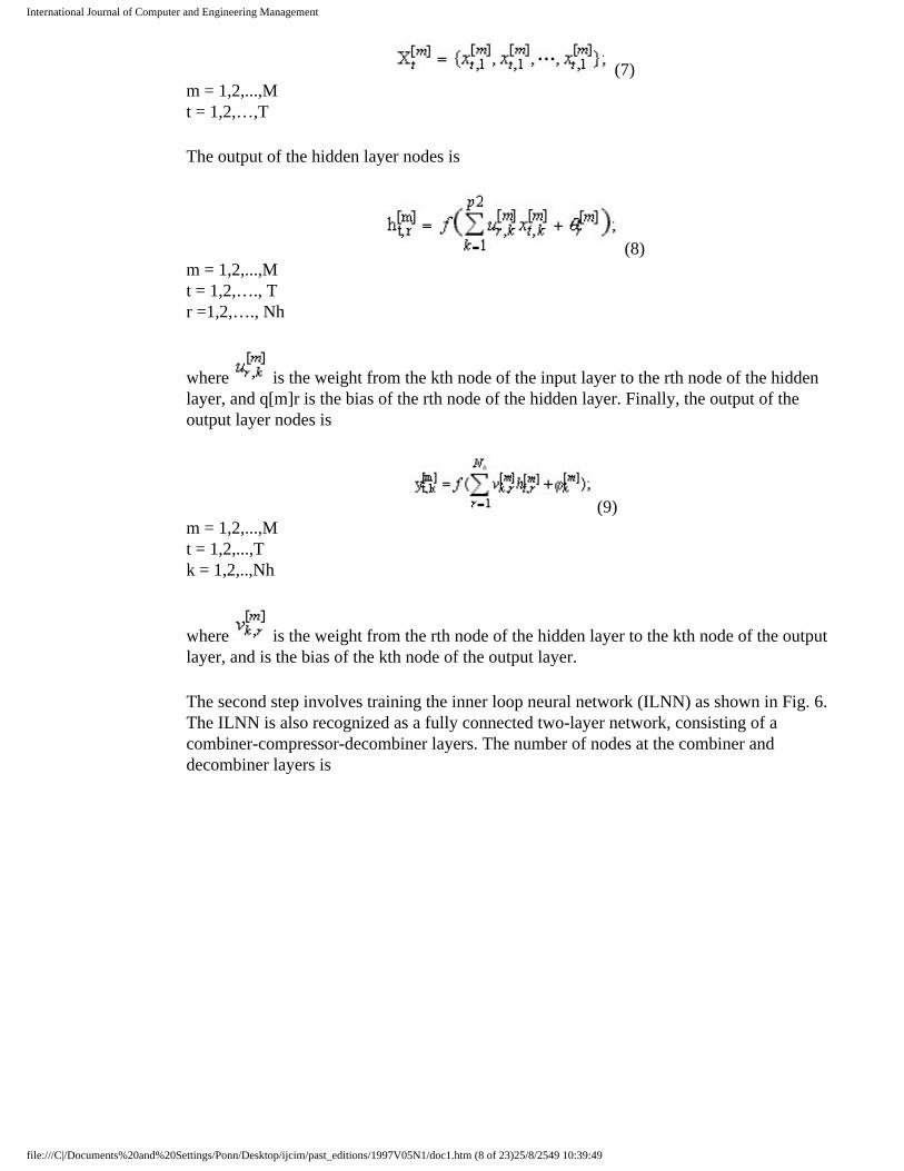
The training procedure for NTA can be broken into 3 steps. The first step involves training the outer loop neural network (OLNN) as shown in Fig. 5. It is recognized as a fully connected symmetric two-layer network, consisting of input-hidden-output layers.The number of nodes at the input and output layer is p2 = 64. The number of hidden layer nodes is Nh = 8. Thus, the OLNN can be considered as 64-8-64 network. Standard backpropagation is used to train each of the OLNN independently in such a way that the desired output equals the input (i e, auto-associative). The connection weights can be obtained after the network converges to an acceptably low error criterion. The training patterns are 8 * 8 patches from each subscene. Hence, the total number of training patterns for each outer loop network is T = 512. The input training set to the network is described as



(7) m = 1,2,...,M t = 1,2,…,T

The output of the hidden layer nodes is

(8) m = 1,2,...,M t = 1,2,…., T r =1,2,…., Nh

where is the weight from the kth node of the input layer to the rth node of the hidden layer, and q[m]r is the bias of the rth node of the hidden layer. Finally, the output of the output layer nodes is

(9) m = 1,2,...,M t = 1,2,...,T k = 1,2,..,Nh

where is the weight from the rth node of the hidden layer to the kth node of the output layer, and is the bias of the kth node of the output layer.

The second step involves training the inner loop neural network (ILNN) as shown in Fig. 6. The ILNN is also recognized as a fully connected two-layer network, consisting of a combiner-compressor-decombiner layers. The number of nodes at the combiner and decombiner layers is



Fig. 5. OLNNs.

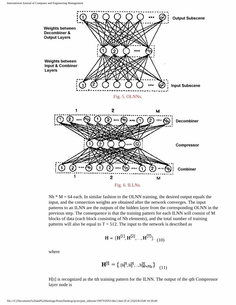
Fig. 6. ILLNs.

Nh * M = 64 each. In similar fashion to the OLNN training, the desired output equals the input, and the connection weights are obtained after the network converges. The input patterns to an ILNN are the outputs of the hidden layer from the corresponding OLNN in the previous step. The consequence is that the training pattern for each ILNN will consist of M blocks of data (each block consisting of Nh elements), and the total number of training patterns will also be equal to T = 512. The input to the network is described as

(10)

where

(11)

H[t] is recognized as the tth training pattern for the ILNN. The output of the qth Compressor layer node is



(12)

where is the weight from the jth node of the combiner layer to the qth node of the compressor layer, and fq is the bias of the qth node of the compressor layer. The output of the dccombiner layer nodes is

(13)

where is the weight from the qth node of the compressor layer to the jth node of the decombiner layer, and Xj is the bias of the jth node of the decombiner layer.

The third and last step involves the reconstruction of the overall network. After the OLNN and ILNN are trained, their trained weights are used to construct the overall network. Since the combiner-compressor-docombiner network for the overall network is the same as the ILNN, the weights obtained from the ILNN are directly transferred to the overall network. Then, we add the input and output layers to the combiner and the decombiner layers, respectively. The connection weights between the input and combiner layers, and the connection weights between decombiner and output layers are obtained as follows. The weights between the mth block of the input layer and mth block of the combiner layers are given by the weights between the input layer and hidden layer of the mth OLNN. Similarly, weights between the mth block of the decombiner and the mth block of the output layer are given by the weights between the hidden layer and the output layer of the mth OLNN.

IV. ANALYTICAL RESULTS

In order to effectively perform data compression, it is important to understand the role of key parameters. In this case, the specification of the learning rate and the network size (which specifies the pixel patch size) are crucial for attaining good performance. These parameters are investigated in detail in the next section.

A. Optimum Learning Rate

The use of the linear activation function allows linear algebra and some tools developed for adaptive signal processing to be applied to the hierarchical neural network. Thus, we restrict our attention to neural network which solely employs linear activation functions. It is noted that the learning constant µ used for network training is analogous to that used in the µ-LMS algorithm [8]. The convergence of the weight vector is ensured if

(14)



where Tr[R] is the summation of the diagonal elements of the correlation matrix R, where R = E[XT X] and X is the input vector. An equivalent viewpoint is that the evolution of the weights can be described in terms of a series product of elementary matrices, where it has been shown that the convergence requirements is identical to that given in (14) [10]. The simulation results provided in Section V uses a value of µ which satisfies the condition given in (14).

B. Optimum Network Size

For the network to be useful, both the ability to learn and generalize are necessary. The network capacity quantifies the learning capabilities at a neural network architecture, which is a measure of the number of training patterns or stimuli that a neural network can correctly identify after training has been completed. Generalization is the ability of the network to correctly identify a pattern on other parts of the domain that the network did not access during the training phase. Thus, while the network capacity is important, it must he accompanied by the ability to generalize. In fact, if generalization is not main objective, one can simply store the association in a look-up table, such as the technique employed in vector quantization. The relationship between generalization and network capacity represents a fundamental tradeoff in neural network applications.

Consider the data compressor described in Section III, which use p * p-dimensional pixel patches as the training patterns for the ILNN and OLNN. Analysis can proceed by considering a two-layer neural network, where the number of nodes in the input and output layers are equal, and the number of nodes in the hidden layer is less than that in the input layer. Let Nx represent the number of nodes in the input layer, Ny represent the number of nodes in the output layer, Nw represent the total number of weights in the network including bias (threshold) weights, and NP represent the total number of patterns in the training set. In order to expect good generalization, it is necessary that the number of training patterns be several times larger than the network capacity, Nw / Ny,, [8,11]. That is,

(15)

Equation (15) can be recast to obtain a generalization constant G which is used to quantify the amount of generalization possible. That is,

(16)

If C represents the network capacity, the low upper bounds on C can be expressed as [8,11]:

(17)

Assume that the training patterns are taken from an N x N pixel scene S, and Nh is the number of hidden nodes. Thus, for the data compression problem.

(18)

If the image is partitioned into p * p pixel patches for training, and each node is assumed to



take on one pixel value, then

(19)

(20) and

(21)

The first term in (21) represents the total number of weights connecting the hidden nodes to the input and output nodes, and the second term represent the connection of the bias weights to the hidden and output nodes. Therefore

(22)

Substituting Np and (Nw / Ny) into (16), we obtain

(23)

The upper bound on network capacity in (17) can be written as:

(24)

From (23) and (24), it can be observed that G and C are inversely related and a tradeoff exists.

We analyze the effect of varying the pixel patch size on G and C for the specific case where K = 0.125 ( i.e ., CR = 8: 1) and the image size is 512 * 512. Equations (23) and (24) can be simplified as

(25) and

(26)

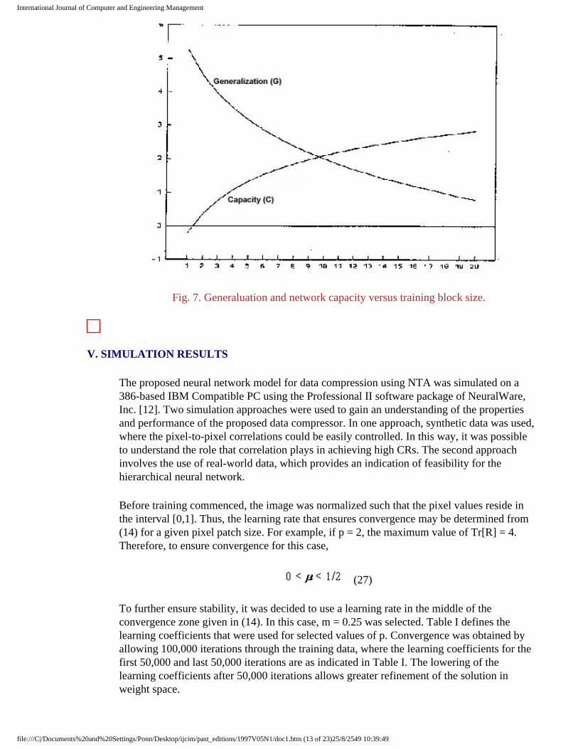
These results are plotted in Fig. 7, which indicate that as the training block size increases, G decreases whereas C increases. This is intuitively pleasing since for larger values of p, (i e, a large pixel patch), the network is able to more easily capture the global feature of the training image, at the expense of its capability to generalize. Fig. 7 also indicates that the optimum training block size is p » 10. The analysis presented here is used to properly interpret the simulation results described in the next section.



Fig. 7. Generaluation and network capacity versus training block size.

V. SIMULATION RESULTS

The proposed neural network model for data compression using NTA was simulated on a 386-based IBM Compatible PC using the Professional II software package of NeuralWare, Inc. [12]. Two simulation approaches were used to gain an understanding of the properties and performance of the proposed data compressor. In one approach, synthetic data was used, where the pixel-to-pixel correlations could be easily controlled. In this way, it was possible to understand the role that correlation plays in achieving high CRs. The second approach involves the use of real-world data, which provides an indication of feasibility for the hierarchical neural network.

Before training commenced, the image was normalized such that the pixel values reside in the interval [0,1]. Thus, the learning rate that ensures convergence may be determined from (14) for a given pixel patch size. For example, if p = 2, the maximum value of Tr[R] = 4. Therefore, to ensure convergence for this case,

(27)

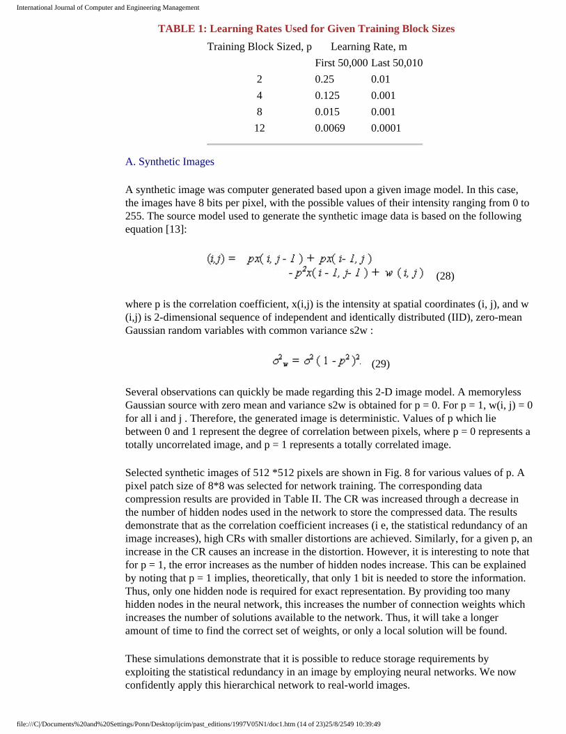
To further ensure stability, it was decided to use a learning rate in the middle of the convergence zone given in (14). In this case, m = 0.25 was selected. Table I defines the learning coefficients that were used for selected values of p. Convergence was obtained by allowing 100,000 iterations through the training data, where the learning coefficients for the first 50,000 and last 50,000 iterations are as indicated in Table I. The lowering of the learning coefficients after 50,000 iterations allows greater refinement of the solution in weight space.



TABLE 1: Learning Rates Used for Given Training Block Sizes

Training Block Sized, p Learning Rate, m

First 50,000 Last 50,010

2 0.25 0.01

4 0.125 0.001

8 0.015 0.001

12 0.0069 0.0001

A. Synthetic Images

A synthetic image was computer generated based upon a given image model. In this case, the images have 8 bits per pixel, with the possible values of their intensity ranging from 0 to 255. The source model used to generate the synthetic image data is based on the following equation [13]:

(28)

where p is the correlation coefficient, x(i,j) is the intensity at spatial coordinates (i, j), and w(i,j) is 2-dimensional sequence of independent and identically distributed (IID), zero-mean Gaussian random variables with common variance s2w :

(29)

Several observations can quickly be made regarding this 2-D image model. A memoryless Gaussian source with zero mean and variance s2w is obtained for p = 0. For p = 1, w(i, j) = 0 for all i and j . Therefore, the generated image is deterministic. Values of p which lie between 0 and 1 represent the degree of correlation between pixels, where p = 0 represents a totally uncorrelated image, and p = 1 represents a totally correlated image.

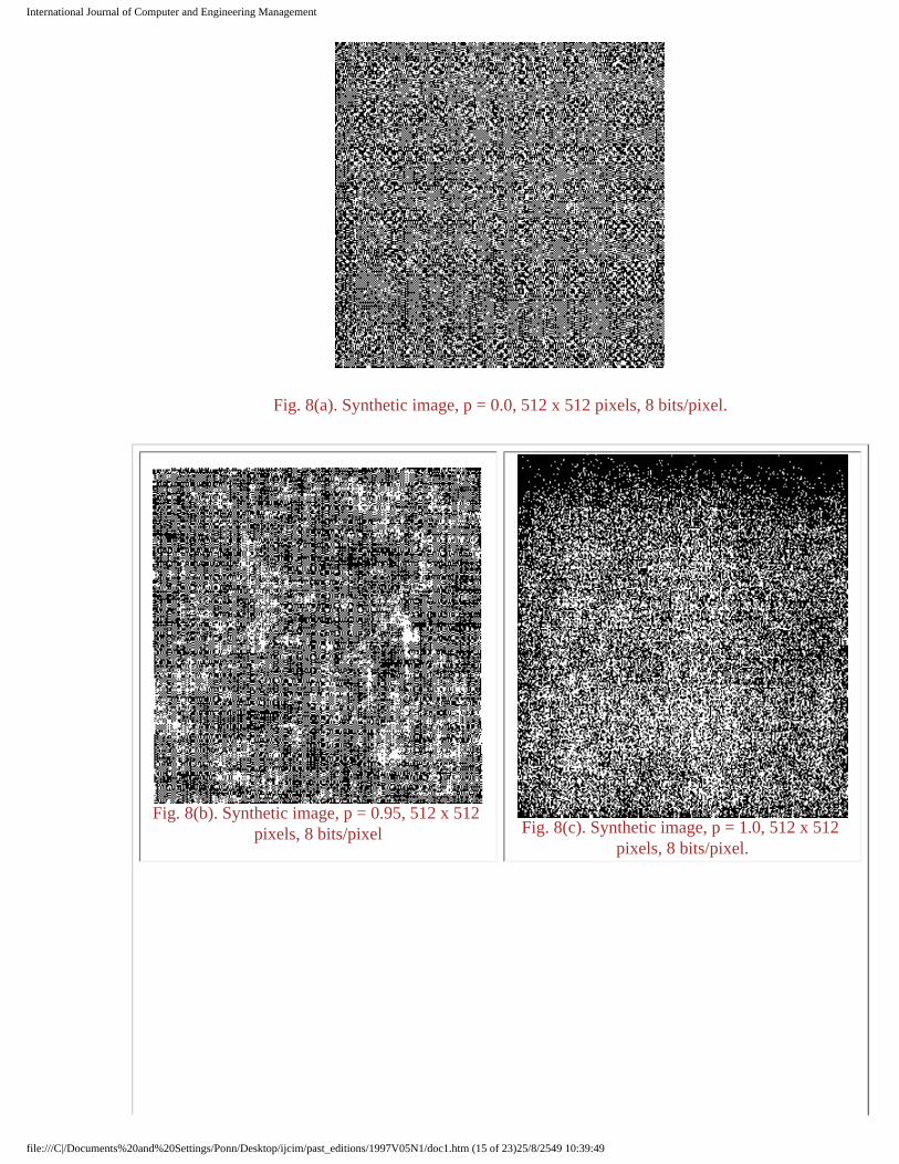
Selected synthetic images of 512 *512 pixels are shown in Fig. 8 for various values of p. A pixel patch size of 8*8 was selected for network training. The corresponding data compression results are provided in Table II. The CR was increased through a decrease in the number of hidden nodes used in the network to store the compressed data. The results demonstrate that as the correlation coefficient increases (i e, the statistical redundancy of an image increases), high CRs with smaller distortions are achieved. Similarly, for a given p, an increase in the CR causes an increase in the distortion. However, it is interesting to note that for p = 1, the error increases as the number of hidden nodes increase. This can be explained by noting that p = 1 implies, theoretically, that only 1 bit is needed to store the information. Thus, only one hidden node is required for exact representation. By providing too many hidden nodes in the neural network, this increases the number of connection weights which increases the number of solutions available to the network. Thus, it will take a longer amount of time to find the correct set of weights, or only a local solution will be found.

These simulations demonstrate that it is possible to reduce storage requirements by exploiting the statistical redundancy in an image by employing neural networks. We now confidently apply this hierarchical network to real-world images.



Fig. 8(a). Synthetic image, p = 0.0, 512 x 512 pixels, 8 bits/pixel.

Fig. 8(b). Synthetic image, p = 0.95, 512 x 512 pixels, 8 bits/pixel

Fig. 8(c). Synthetic image, p = 1.0, 512 x 512 pixels, 8 bits/pixel.



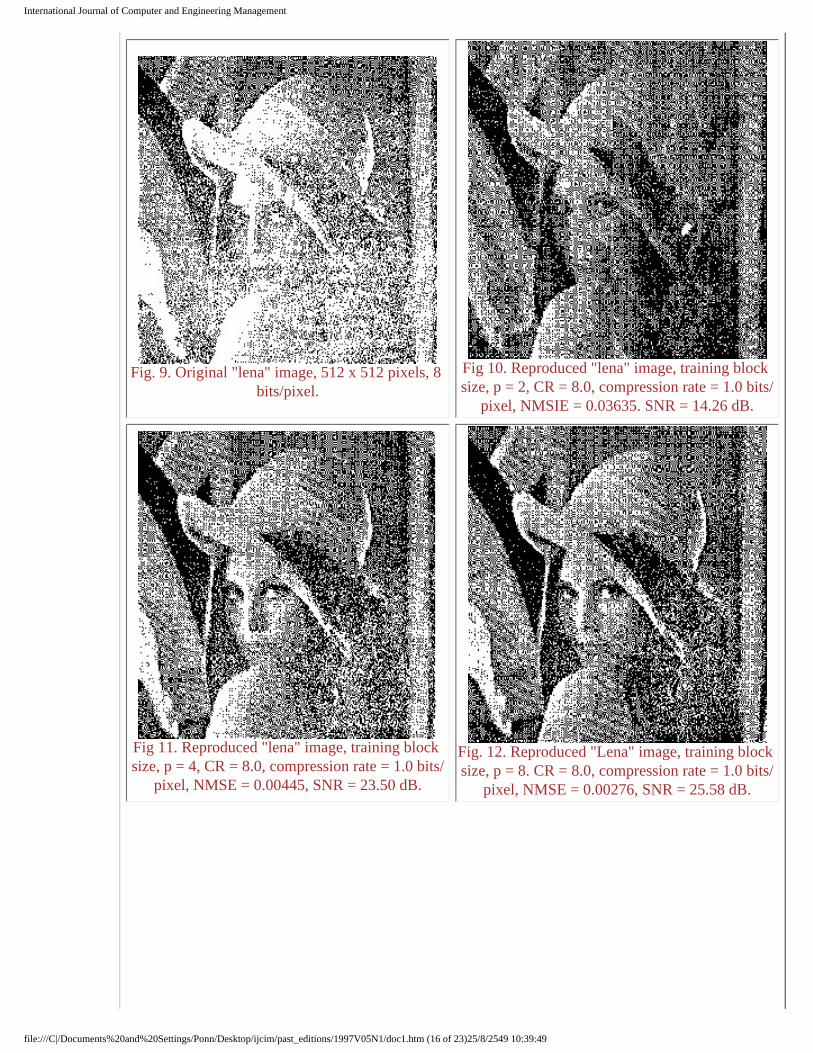
Fig. 9. Original "lena" image, 512 x 512 pixels, 8 bits/pixel.

Fig 10. Reproduced "lena" image, training block size, p = 2, CR = 8.0, compression rate = 1.0 bits/

pixel, NMSIE = 0.03635. SNR = 14.26 dB.

Fig 11. Reproduced "lena" image, training block size, p = 4, CR = 8.0, compression rate = 1.0 bits/

pixel, NMSE = 0.00445, SNR = 23.50 dB.

Fig. 12. Reproduced "Lena" image, training block size, p = 8. CR = 8.0, compression rate = 1.0 bits/

pixel, NMSE = 0.00276, SNR = 25.58 dB.



Fig. 13. Reproduced "lena" image, training block size, p = 12, CR = 8.0, compression rate = 1.0 bits/pixel, NMSE = 0.00271, SNR = 25.66 dB.

Flg. 14. Original "mandrill" image, 512 x 512 pixels, 8 bits/pixel

Fig. 15 Reproduced "mandrill" image, training block size, p = 2, CR= 8.0, compression rate = 1.0 bits/pixel, NMSE = 0.06518, SNR = 11.87

dB.

Fig. 16. Reproduced "mandrill image, training block size, p = 4, CR = 8.0, compression rate =

10 bits/pixel, NMSE = 0.01685, SNR = 17.66 dB.



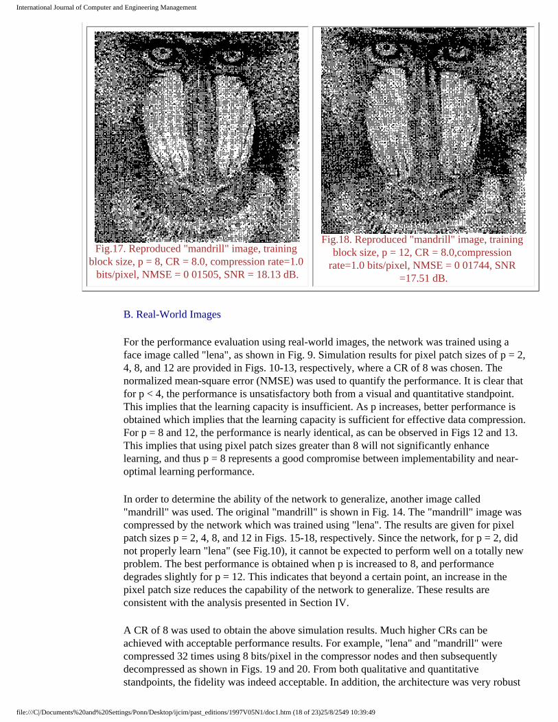
Fig.17. Reproduced "mandrill" image, training block size, p = 8, CR = 8.0, compression rate=1.0

bits/pixel, NMSE = 0 01505, SNR = 18.13 dB.

Fig.18. Reproduced "mandrill" image, training block size, p = 12, CR = 8.0,compression

rate=1.0 bits/pixel, NMSE = 0 01744, SNR =17.51 dB.

B. Real-World Images

For the performance evaluation using real-world images, the network was trained using a face image called "lena", as shown in Fig. 9. Simulation results for pixel patch sizes of p = 2, 4, 8, and 12 are provided in Figs. 10-13, respectively, where a CR of 8 was chosen. The normalized mean-square error (NMSE) was used to quantify the performance. It is clear that for p < 4, the performance is unsatisfactory both from a visual and quantitative standpoint. This implies that the learning capacity is insufficient. As p increases, better performance is obtained which implies that the learning capacity is sufficient for effective data compression. For p = 8 and 12, the performance is nearly identical, as can be observed in Figs 12 and 13. This implies that using pixel patch sizes greater than 8 will not significantly enhance learning, and thus p = 8 represents a good compromise between implementability and near-optimal learning performance.

In order to determine the ability of the network to generalize, another image called "mandrill" was used. The original "mandrill" is shown in Fig. 14. The "mandrill" image was compressed by the network which was trained using "lena". The results are given for pixel patch sizes p = 2, 4, 8, and 12 in Figs. 15-18, respectively. Since the network, for p = 2, did not properly learn "lena" (see Fig.10), it cannot be expected to perform well on a totally new problem. The best performance is obtained when p is increased to 8, and performance degrades slightly for p = 12. This indicates that beyond a certain point, an increase in the pixel patch size reduces the capability of the network to generalize. These results are consistent with the analysis presented in Section IV.

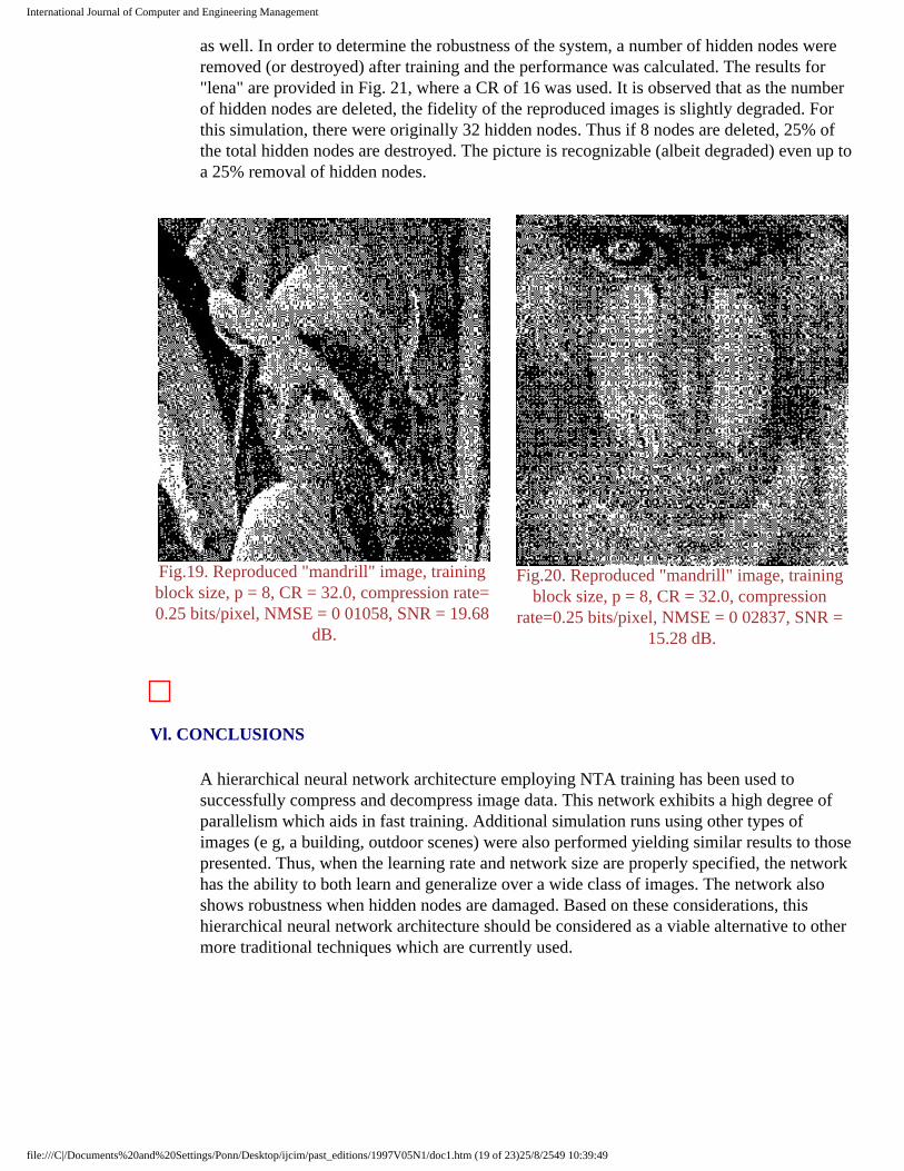
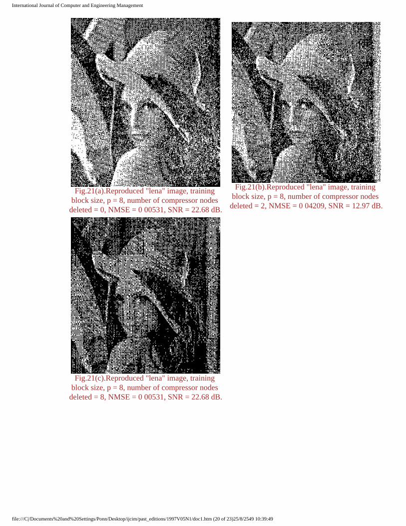
A CR of 8 was used to obtain the above simulation results. Much higher CRs can be achieved with acceptable performance results. For example, "lena" and "mandrill" were compressed 32 times using 8 bits/pixel in the compressor nodes and then subsequently decompressed as shown in Figs. 19 and 20. From both qualitative and quantitative standpoints, the fidelity was indeed acceptable. In addition, the architecture was very robust



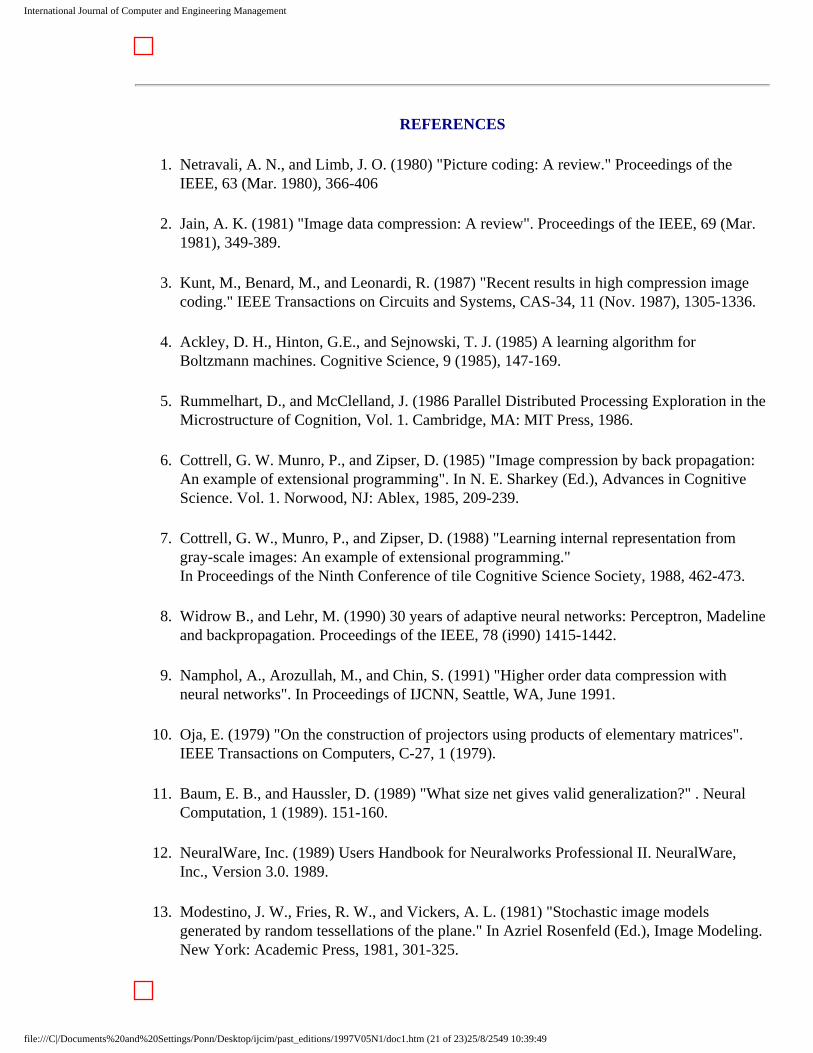
as well. In order to determine the robustness of the system, a number of hidden nodes were removed (or destroyed) after training and the performance was calculated. The results for "lena" are provided in Fig. 21, where a CR of 16 was used. It is observed that as the number of hidden nodes are deleted, the fidelity of the reproduced images is slightly degraded. For this simulation, there were originally 32 hidden nodes. Thus if 8 nodes are deleted, 25% of the total hidden nodes are destroyed. The picture is recognizable (albeit degraded) even up to a 25% removal of hidden nodes.

Fig.19. Reproduced "mandrill" image, training block size, p = 8, CR = 32.0, compression rate= 0.25 bits/pixel, NMSE = 0 01058, SNR = 19.68

dB.

Fig.20. Reproduced "mandrill" image, training block size, p = 8, CR = 32.0, compression

rate=0.25 bits/pixel, NMSE = 0 02837, SNR = 15.28 dB.

Vl. CONCLUSIONS

A hierarchical neural network architecture employing NTA training has been used to successfully compress and decompress image data. This network exhibits a high degree of parallelism which aids in fast training. Additional simulation runs using other types of images (e g, a building, outdoor scenes) were also performed yielding similar results to those presented. Thus, when the learning rate and network size are properly specified, the network has the ability to both learn and generalize over a wide class of images. The network also shows robustness when hidden nodes are damaged. Based on these considerations, this hierarchical neural network architecture should be considered as a viable alternative to other more traditional techniques which are currently used.



Fig.21(a).Reproduced "lena" image, training block size, p = 8, number of compressor nodes

deleted = 0, NMSE = 0 00531, SNR = 22.68 dB.

Fig.21(b).Reproduced "lena" image, training block size, p = 8, number of compressor nodes


Fig.21(c).Reproduced "lena" image, training block size, p = 8, number of compressor nodes




REFERENCES

1. Netravali, A. N., and Limb, J. O. (1980) "Picture coding: A review." Proceedings of the IEEE, 63 (Mar. 1980), 366-406

2. Jain, A. K. (1981) "Image data compression: A review". Proceedings of the IEEE, 69 (Mar. 1981), 349-389.

3. Kunt, M., Benard, M., and Leonardi, R. (1987) "Recent results in high compression image coding." IEEE Transactions on Circuits and Systems, CAS-34, 11 (Nov. 1987), 1305-1336.

4. Ackley, D. H., Hinton, G.E., and Sejnowski, T. J. (1985) A learning algorithm for Boltzmann machines. Cognitive Science, 9 (1985), 147-169.

5. Rummelhart, D., and McClelland, J. (1986 Parallel Distributed Processing Exploration in the Microstructure of Cognition, Vol. 1. Cambridge, MA: MIT Press, 1986.

6. Cottrell, G. W. Munro, P., and Zipser, D. (1985) "Image compression by back propagation: An example of extensional programming". In N. E. Sharkey (Ed.), Advances in Cognitive Science. Vol. 1. Norwood, NJ: Ablex, 1985, 209-239.

7. Cottrell, G. W., Munro, P., and Zipser, D. (1988) "Learning internal representation from gray-scale images: An example of extensional programming." In Proceedings of the Ninth Conference of tile Cognitive Science Society, 1988, 462-473.

8. Widrow B., and Lehr, M. (1990) 30 years of adaptive neural networks: Perceptron, Madeline and backpropagation. Proceedings of the IEEE, 78 (i990) 1415-1442.

9. Namphol, A., Arozullah, M., and Chin, S. (1991) "Higher order data compression with neural networks". In Proceedings of IJCNN, Seattle, WA, June 1991.

10. Oja, E. (1979) "On the construction of projectors using products of elementary matrices". IEEE Transactions on Computers, C-27, 1 (1979).

11. Baum, E. B., and Haussler, D. (1989) "What size net gives valid generalization?" . Neural Computation, 1 (1989). 151-160.

12. NeuralWare, Inc. (1989) Users Handbook for Neuralworks Professional II. NeuralWare, Inc., Version 3.0. 1989.

13. Modestino, J. W., Fries, R. W., and Vickers, A. L. (1981) "Stochastic image models generated by random tessellations of the plane." In Azriel Rosenfeld (Ed.), Image Modeling. New York: Academic Press, 1981, 301-325.



About the Authors

Aran Namphol received the BEE, MEE, and Ph D in electrical engineering, from the Catholic University of America, Washington, DC, in 1987, 1989, and 1992, respectively.

He is currently working with thc Royal Thai Navy at the Communications Division. He is also engaged in teaching at the Assumption University in Bangkok, Thailand, in the areas of computer networks and operations research. His research interests include neural networks and performance analysis of communication networks

Steven H. Chin was born in Bronx, NY. He received the B S. in electrical engineering from Rutgers University, New Brunswick, NJ, in 1979, the M.S.E.E from The Johns Hopkins University, Baltimore, MD, in 1982, and the Ph.D degree in electrical engineering in 1987 from Rutgers University.

He joined the Department of Electrical Engineering at the Catholic University of America, Washington, DC, in 1988, where he is currently a lecturer in the Electrical Engineering Department, and also serves as the Assistant Dean in the School of Engineering. His research interests include application of neural networks, signal processing, and computer networking

Mohammed Arozullah received his undergraduate education in Bangladesh. He received the M.Sc. and Ph.D in electrical engineering from the University of Ottawa, Ottawa Canada.

He was a faculty member in the Electrical Engineering Department of Queen's University in Kingston, Ontario, Canada from 1967 to 1969. He was on the faculty of Electrical and Computer Engineering of Clarkson University in Potsdam, NY from 1969 to 1981. Since 1981, he has been with the Electrical Engineering Department at the Catholic University of America in Washington, DC where he is currently a Professor of Electrical Engineering and Director of Communication and Information Concentration. His research interests include computer communication networks, multiple satellite networks, and neural networks.

Authors' current addresses:

A. Namphol, Assumption University, Bangkok, Thailand;

S. H. Chin and M. Arozullah, Dept. of Electrical Engineering, Catholic University of America, Washington, DC 20064.
