ODF RECONSTRUCTION IN Q-BALL IMAGING WITH

SOLID ANGLE CONSIDERATION

By

Iman Aganj

Christophe Lenglet

and

Guillermo Sapiro

IMA Preprint Series # 2233

( January 2009 )

INSTITUTE FOR MATHEMATICS AND ITS APPLICATIONS

UNIVERSITY OF MINNESOTA

400 Lind Hall207 Church Street S.E.

Minneapolis, Minnesota 55455–0436Phone: 612/624-6066 Fax: 612/626-7370

URL: http://www.ima.umn.edu

(a) (b)

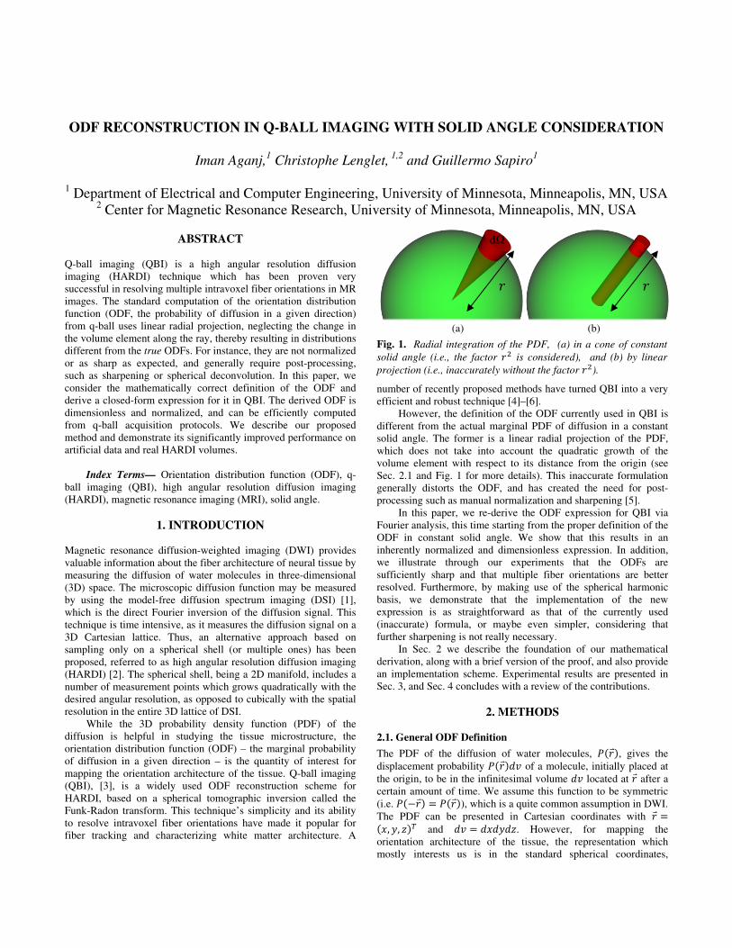
Fig. 1. Radial integration of the PDF, (a) in a cone of constant

solid angle (i.e., the factor is considered), and (b) by linear

projection (i.e., inaccurately without the factor ).

ODF RECONSTRUCTION IN Q-BALL IMAGING WITH SOLID ANGLE CONSIDERATION

Iman Aganj,

1 Christophe Lenglet,

1,2 and Guillermo Sapiro

1

1 Department of Electrical and Computer Engineering, University of Minnesota, Minneapolis, MN, USA

2 Center for Magnetic Resonance Research, University of Minnesota, Minneapolis, MN, USA

ABSTRACT

Q-ball imaging (QBI) is a high angular resolution diffusion imaging (HARDI) technique which has been proven very successful in resolving multiple intravoxel fiber orientations in MR images. The standard computation of the orientation distribution function (ODF, the probability of diffusion in a given direction) from q-ball uses linear radial projection, neglecting the change in the volume element along the ray, thereby resulting in distributions different from the true ODFs. For instance, they are not normalized or as sharp as expected, and generally require post-processing, such as sharpening or spherical deconvolution. In this paper, we consider the mathematically correct definition of the ODF and derive a closed-form expression for it in QBI. The derived ODF is dimensionless and normalized, and can be efficiently computed from q-ball acquisition protocols. We describe our proposed method and demonstrate its significantly improved performance on artificial data and real HARDI volumes.

Index Terms— Orientation distribution function (ODF), q-ball imaging (QBI), high angular resolution diffusion imaging (HARDI), magnetic resonance imaging (MRI), solid angle.

1. INTRODUCTION Magnetic resonance diffusion-weighted imaging (DWI) provides valuable information about the fiber architecture of neural tissue by measuring the diffusion of water molecules in three-dimensional (3D) space. The microscopic diffusion function may be measured by using the model-free diffusion spectrum imaging (DSI) [1], which is the direct Fourier inversion of the diffusion signal. This technique is time intensive, as it measures the diffusion signal on a 3D Cartesian lattice. Thus, an alternative approach based on sampling only on a spherical shell (or multiple ones) has been proposed, referred to as high angular resolution diffusion imaging (HARDI) [2]. The spherical shell, being a 2D manifold, includes a number of measurement points which grows quadratically with the desired angular resolution, as opposed to cubically with the spatial resolution in the entire 3D lattice of DSI.

While the 3D probability density function (PDF) of the diffusion is helpful in studying the tissue microstructure, the orientation distribution function (ODF) – the marginal probability of diffusion in a given direction – is the quantity of interest for mapping the orientation architecture of the tissue. Q-ball imaging (QBI), [3], is a widely used ODF reconstruction scheme for HARDI, based on a spherical tomographic inversion called the Funk-Radon transform. This technique’s simplicity and its ability to resolve intravoxel fiber orientations have made it popular for fiber tracking and characterizing white matter architecture. A

number of recently proposed methods have turned QBI into a very efficient and robust technique [4]–[6].

However, the definition of the ODF currently used in QBI is different from the actual marginal PDF of diffusion in a constant solid angle. The former is a linear radial projection of the PDF, which does not take into account the quadratic growth of the volume element with respect to its distance from the origin (see Sec. 2.1 and Fig. 1 for more details). This inaccurate formulation generally distorts the ODF, and has created the need for post-processing such as manual normalization and sharpening [5].

In this paper, we re-derive the ODF expression for QBI via Fourier analysis, this time starting from the proper definition of the ODF in constant solid angle. We show that this results in an inherently normalized and dimensionless expression. In addition, we illustrate through our experiments that the ODFs are sufficiently sharp and that multiple fiber orientations are better resolved. Furthermore, by making use of the spherical harmonic basis, we demonstrate that the implementation of the new expression is as straightforward as that of the currently used (inaccurate) formula, or maybe even simpler, considering that further sharpening is not really necessary.

In Sec. 2 we describe the foundation of our mathematical derivation, along with a brief version of the proof, and also provide an implementation scheme. Experimental results are presented in Sec. 3, and Sec. 4 concludes with a review of the contributions.

2. METHODS 2.1. General ODF Definition

The PDF of the diffusion of water molecules, , gives the displacement probability of a molecule, initially placed at the origin, to be in the infinitesimal volume located at after a certain amount of time. We assume this function to be symmetric (i.e. − = ), which is a quite common assumption in DWI. The PDF can be presented in Cartesian coordinates with =, , and = . However, for mapping the orientation architecture of the tissue, the representation which mostly interests us is in the standard spherical coordinates,

dΩ

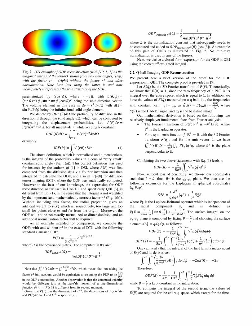
Fig. 2. DTI example of ODF reconstruction (with 10, 5, 1 as the

diagonal entries of the tensor), shown from two view angles, (left)

with the factor , (right) without the factor and after

normalization. Note how less sharp the latter is and how

incompletely it represents the true structure of the ODF.

parameterized by , , , where = , with , =sin cos , sin sin , cos being the unit direction vector. The volume element in this case is = Ω with Ω =sin being the infinitesimal solid angle element.

We denote by Ω the probability of diffusion in the direction through the solid angle Ω, which can be computed by integrating the displacement probabilities, i.e., =Ω, for all magnitude , while keeping constant:

Ω = Ω∞

or simply:

= ∞

(1)

The above definition, which is normalized and dimensionless, is the integral of the probability values in a cone of “very small” constant solid angle (Fig. 1(a)). This correct definition was used for instance by the authors of [1] in DSI, where was first computed from the diffusion data via Fourier inversion and then integrated to calculate the ODF, and also in [7]–[8] for diffusion tensor imaging (DTI), where the ODF was analytically computed. However to the best of our knowledge, the expression for ODF reconstruction so far used in HARDI, and specifically QBI [3], is different from Eq. (1), in the sense that the integral is not weighted by the important (and mathematically correct) factor (Fig. 1(b)). Without including this factor, the radial projection gives an artificial weight to which is, respectively, too large and too small for points close to and far from the origin.1 Moreover, the ODF will not be necessarily normalized or dimensionless,2 and an additional normalization factor will be required.

As an example intended for comparison, we compute the ODFs with and without in the case of DTI, with the following standard Gaussian PDF: =

!"#|%|&# '(&#)%*& where is the covariance matrix. The computed ODFs are:

+,-. # = 142|| ( 34

1 Note that 5 ∞ = 5 678# ∞ , which means that not taking the

factor into account would be equivalent to assuming the PDF to be 6||#

in the ODF computation. Another observation is that the computed quantity would be different just as the zero’th moment of a one-dimensional function 9 ≔ is different from its second moment. 2 Given that has the dimension of ;(<, the dimensions of and are 1 and ;(, respectively.

+,-.=7- # = 1> 142|| ( ?4

where > is the normalization constant that subsequently needs to be computed and added to +,-.=7- # (see [3]). An example of this pair of ODFs is illustrated in Fig. 2. No min-max normalization is used in any of the figures.

Next, we derive a closed-form expression for the ODF in QBI using the correct -weighted integral.

2.2. Q-ball Imaging ODF Reconstruction

We present here a brief version of the proof for the ODF expression in QBI. The complete proof is provided in [9].

Let @A be the 3D Fourier transform of . Theoretically, we know that @0 = 1, since the zero frequency of a PDF is its integral over the entire space, which is equal to 1. In addition, we have the values of @A measured on a q-ball, i.e., the frequencies

with constant norm |A| = A, as @C ≔ @A = D78DE , where F is the HARDI signal and F is the base-line image. Our mathematical derivation is based on the following two

relatively simple yet fundamental facts from Fourier analysis: • The Fourier transform of || is −∇@A, where ∇ is the Laplacian operator.

• For a symmetric function H: ℝ< → ℝ with the 3D Fourier

transform A, and for the unit vector , we have 5 H∞ = L!# M AA78N , where O is the plane

perpendicular to .

Combining the two above statements with Eq. (1) leads to

= − 182 Q ∇@AA78N

Now, without loss of generality, we choose our coordinates such that = , thus O is the AS-AT plane. We then use the following expansion for the Laplacian in spherical coordinates A, , :

∇@ = 1A UUA A@ + 1A ∇W@

where ∇W is the Laplace-Beltrami operator which is independent of the radial component A, and is defined as ∇W@ = XYZ [ \\[ ]sin \^\[_ + XYZ# [ \#^\`#. The surface integral on the

AS-AT plane is computed by fixing = ! and choosing the surface

element A = AA, as follows:

= − 182 ∇@AAA∞

!

= − 182 a1A UUA A@ + 1A ∇W@b AA∞

!

One can verify that the integral of the first term is independent of @A and its derivatives:

c1A UUA A@d AA∞

! = −22@0 = −22

Therefore:

= 142 − 182 1A ∇W@AA∞

!

while = ! is kept constant in the integration.

To compute the integral of the second term, the values of @A are required for the entire q-space, which except for the time-

consuming DSI modality, are not available. Thus, we need to approximate @A from the values measured on the q-ball. In this work, we consider the following radial mono-exponential model:

@A ≅ @Ag#gE# = @Cg#gE# where A is the radius of the q-ball. This type of interpolation has been previously used and discussed in [10]–[11].3 After applying the mono-exponential assumption and a few more steps of calculations, the following ODF expression can be derived:

= 142 + 1162 ∇W lnj− ln @Ck !

Finally, rewriting the expression independently of the choice of the axes, the following analytical formula can be shown to hold for the ODF:

lmno8 = ?pq + ??rq4 nstuvw4 xyj− xy zo8k| (2)

where ~ is the Funk-Radon transform [12], defined as:

~H ≔ Q H|| − 178N

with ∙ being the Dirac delta function. We can see that the above ODF expression is dimensionless

and intrinsically normalized, as the integrals of the first and second terms over the sphere are 1 and 0, respectively. This is in contrast

to the ODF formula originally used in QBI, i.e., ~@C,

where a normalization factor > was needed. 2.3. Implementation

Our implementation of the ODF reconstruction makes use of the spherical harmonic (SH) basis, , which is quite common for the analysis of HARDI data. The steps taken here to numerically compute Eq. (2) are similar to those described in [5], except that no regularization or sharpening is performed (regularizations will further improve the results). Particularly, we use the real and symmetric modified SH basis introduced in [5], where SH functions are indexed by a single parameter corresponding to and .

We first employ a minimum least square scheme to compute the modified SH coefficients of the double logarithm of the signal, such that

lnj− ln @Ck ≈

where = + 1 + 2/2, with being the order of the SH basis (we chose = 4 throughout our experiments). Next, since the SH elements are eigenfunctions of the Laplace-Beltrami operator, we compute ∇W lnj− ln @Ck by multiplying the coefficients by

their corresponding eigenvalues, – j + 1k. Then, as suggested in [5], the Funk-Radon transform is computed by multiplying the coefficients by 220, where ∙ is the Legendre polynomial

of degree , with 0 = −1# ×<×⋯×( ××⋯× for even . Finally,

since = √!, the SH coefficients of the ODF are derived as

′ = 12√2 = 1

− 182 −1 1 × 3 × ⋯ × j + 1k2 × 4 × ⋯ × j − 2k > 1 3 An advantage of the model used here over the original QBI model, i.e. @A ≅ @CA − A, is the compatibility with @0 = 1.

As can be seen, by taking advantage of the SH framework, this implementation is as straightforward as the one introduced in [5] for the original QBI ODF formula, or even simpler if no further sharpening is to be performed.

3. RESULTS AND DISCUSSION To validate our approach, we first show results using artificial data. We simulated fiber crossing by synthesizing diffusion images from

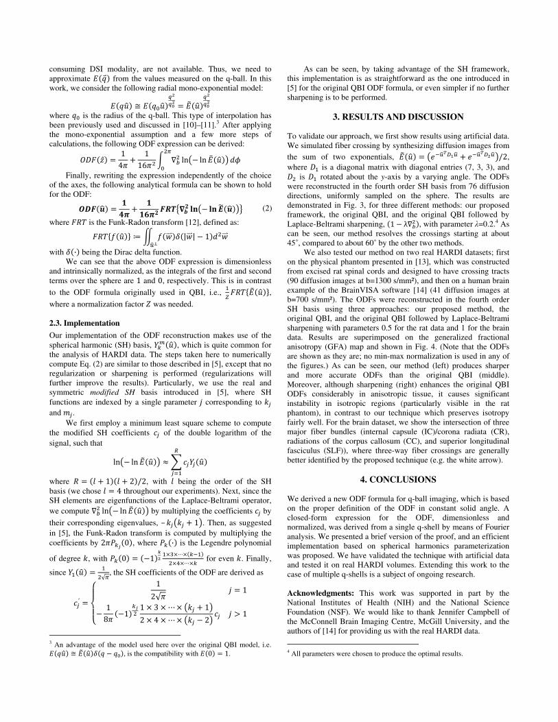
the sum of two exponentials, @C = j'(78)%&78 + '(78)%#78k/2, where is a diagonal matrix with diagonal entries (7, 3, 3), and is rotated about the y-axis by a varying angle. The ODFs were reconstructed in the fourth order SH basis from 76 diffusion directions, uniformly sampled on the sphere. The results are demonstrated in Fig. 3, for three different methods: our proposed framework, the original QBI, and the original QBI followed by Laplace-Beltrami sharpening, 1 − λ∇W, with parameter λ=0.2.4 As can be seen, our method resolves the crossings starting at about 45˚, compared to about 60˚ by the other two methods.

We also tested our method on two real HARDI datasets; first on the physical phantom presented in [13], which was constructed from excised rat spinal cords and designed to have crossing tracts (90 diffusion images at b=1300 s/mm²), and then on a human brain example of the BrainVISA software [14] (41 diffusion images at b=700 s/mm²). The ODFs were reconstructed in the fourth order SH basis using three approaches: our proposed method, the original QBI, and the original QBI followed by Laplace-Beltrami sharpening with parameters 0.5 for the rat data and 1 for the brain data. Results are superimposed on the generalized fractional anisotropy (GFA) map and shown in Fig. 4. (Note that the ODFs are shown as they are; no min-max normalization is used in any of the figures.) As can be seen, our method (left) produces sharper and more accurate ODFs than the original QBI (middle). Moreover, although sharpening (right) enhances the original QBI ODFs considerably in anisotropic tissue, it causes significant instability in isotropic regions (particularly visible in the rat phantom), in contrast to our technique which preserves isotropy fairly well. For the brain dataset, we show the intersection of three major fiber bundles (internal capsule (IC)/corona radiata (CR), radiations of the corpus callosum (CC), and superior longitudinal fasciculus (SLF)), where three-way fiber crossings are generally better identified by the proposed technique (e.g. the white arrow).

4. CONCLUSIONS

We derived a new ODF formula for q-ball imaging, which is based on the proper definition of the ODF in constant solid angle. A closed-form expression for the ODF, dimensionless and normalized, was derived from a single q-shell by means of Fourier analysis. We presented a brief version of the proof, and an efficient implementation based on spherical harmonics parameterization was proposed. We have validated the technique with artificial data and tested it on real HARDI volumes. Extending this work to the case of multiple q-shells is a subject of ongoing research. Acknowledgments: This work was supported in part by the National Institutes of Health (NIH) and the National Science Foundation (NSF). We would like to thank Jennifer Campbell of the McConnell Brain Imaging Centre, McGill University, and the authors of [14] for providing us with the real HARDI data.

4 All parameters were chosen to produce the optimal results.

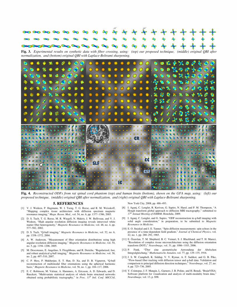
Fig. 3. Experimental results on synthetic data with fiber crossing, using: (top) our proposed technique, (middle) original QBI after

normalization, and (bottom) original QBI with Laplace-Beltrami sharpening.

Fig. 4. Reconstructed ODFs from rat spinal cord phantom (top) and human brain (bottom), shown on the GFA map, using: (left) our

proposed technique, (middle) original QBI after normalization, and (right) original QBI with Laplace-Beltrami sharpening.

5. REFERENCES

[1] V. J. Wedeen, P. Hagmann, W. I. Tseng, T. G. Reese, and R. M. Weisskoff, “Mapping complex tissue architecture with diffusion spectrum magnetic resonance imaging,” Magn. Reson. Med., vol. 54, no. 6, pp. 1377–1386, 2005.

[2] D. S. Tuch, T. G. Reese, M. R. Wiegell, N. Makris, J. W. Belliveau, and V. J. Wedeen, “High angular resolution diffusion imaging reveals intravoxel white matter fiber heterogeneity,” Magnetic Resonance in Medicine, vol. 48, no. 4, pp. 577–582, 2002.

[3] D. S. Tuch, “Q-ball imaging,” Magnetic Resonance in Medicine, vol. 52, no. 6, pp. 1358–1372, 2004.

[4] A. W. Anderson, “Measurement of fiber orientation distributions using high angular resolution diffusion imaging,” Magnetic Resonance in Medicine, vol. 54, no. 5, pp. 1194–1206, 2005.

[5] M. Descoteaux, E. Angelino, S. Fitzgibbons, and R. Deriche, “Regularized, fast, and robust analytical q-ball imaging,” Magnetic Resonance in Medicine, vol. 58, no. 2, pp. 497–510, 2007.

[6] C. P. Hess, P. Mukherjee, E. T. Han, D. Xu, and D. B. Vigneron, “Q-ball reconstruction of multimodal fiber orientations using the spherical harmonic basis,” Magnetic Resonance in Medicine, vol. 56, no. 1, pp. 104–117, 2006.

[7] E. C. Robinson, M. Valstar, A. Hammers, A. Ericsson, A. D. Edwards, and D. Rueckert, “Multivariate statistical analysis of whole brain structural networks obtained using probabilistic tractography,” in Proc. 11th Intl. Conf. MICCAI,

New York City, 2008, pp. 486–493.

[8] I. Aganj, C. Lenglet, R. Keriven, G. Sapiro, N. Harel, and P. M. Thompson, “A Hough transform global approach to diffusion MRI tractography,” submitted to

17th Annual Meeting of ISMRM, Honolulu, 2009.

[9] I. Aganj, C. Lenglet, and G. Sapiro, “ODF reconstruction in q-ball imaging with solid angle consideration,” in preparation, to be submitted to Magnetic

Resonance in Medicine.

[10] E. O. Stejskal and J. E. Tanner, “Spin diffusion measurements: spin echoes in the presence of a time-dependent field gradient,” Journal of Chemical Physics, vol. 42, no. 1, pp. 288–292, 1965.

[11] E. Özarslan, T. M. Shepherd, B. C. Vemuri, S. J. Blackband, and T. H. Mareci, “Resolution of complex tissue microarchitecture using the diffusion orientation transform (DOT),” NeuroImage, vol. 31, pp. 1086–1103, 2006.

[12] P. Funk, “Über eine geometrische Anwendung der Abelschen Integralgleichung,” Mathematische Annalen, vol. 77, pp. 129–135, 1916.

[13] J. S. W. Campbell, K. Siddiqi, V. V. Rymar, A. F. Sadikot, and G. B. Pike, “Flow-based fiber tracking with diffusion tensor and q-ball data: Validation and comparison to principal diffusion direction techniques,” NeuroImage, vol. 27, no. 4, pp. 725–736, 2005.

[14] Y. Cointepas, J. F. Mangin, L. Garnero, J. B. Poline, and H. Benali, “BrainVISA: Software platform for visualization and analysis of multi-modality brain data,” NeuroImage, vol. 13, p. S98.

45˚

SLF

IC

60˚

CR

CC

CSF