ima paule radu - risc.jku.at · peter paule and silviu radu abstract. this article describes recent...
TRANSCRIPT

PARTITION ANALYSIS, MODULAR FUNCTIONS, AND
COMPUTER ALGEBRA
PETER PAULE AND SILVIU RADU
Abstract. This article describes recent developments connecting problems
of enumerative combinatorics, constrained by linear systems of Diophantineinequalities, with number theory topics like partitions, partition congruences,and q-series identities. Special emphasis is put on the role of computer algebra
algorithms. The presentation is intended for a broader audience; to this end,elementary introductions to notions like modular functions and to algorithmicaspects of algebra are given.
1. Introduction
As indicated by the title, this article has a relatively wide topical range which reachesfrom enumerative combinatorics and linear systems of Diophantine inequalities tonumber theoretic themes like partitions, partition congruences, and q-series identi-ties. From the methods point of view, despite relying also on analytic concepts likemodular functions, special emphasis is put on transforming the analytic frameworkinto algebra, in particular, into computer algebra tools like the Ramanujan-Kolbergpackage to compute q-identities as witnesses for divisibility properties of partitionnumbers. The underlying mathematics of the Omega package is more on the alge-braic side: semigroups, posets, etc. Omega is an implementation of MacMahon’smethod of partition analysis, having strong connections also to aspects of discretegeometry. The objective of this article is to provide an introduction to several recentdevelopments and trends in these areas. The explanatory style of the exposition ischosen to attract also non-expert readers.
To illustrate the possible scope of applications, we quote a problem from Polya [21,Example 5]: “The three sides of a triangle are of lengths l, m, and n, respectively.The numbers l, m, and n are positive integers, l ≤ m ≤ n. Find the number ofdifferent triangles of the described kind for a given n. Find a general law governingthe dependence of the number of triangles on n.” The answer to this problem canbe easily extracted from
∑
1≤a≤b≤cs.t. a + b > c
xaybzc =xyz
(1− yz)(1− xyz)(1− xyz2),
a relation which, as explained with other examples below, can be easily computedwith the Omega package; see also [5]. Apart from elementary problems like this,partition analysis can be used in far more challenging contexts, for instance, as weshall see in Section 3 for the construction of combinatorial objects having modularforms as generating functions.
The research of Radu was supported by the strategic program “Innovatives OO 2010 plus” bythe Upper Austrian Government in the frame of project W1214-N15-DK6 of the Austrian Science
Fund (FWF).
1
2 PETER PAULE AND SILVIU RADU
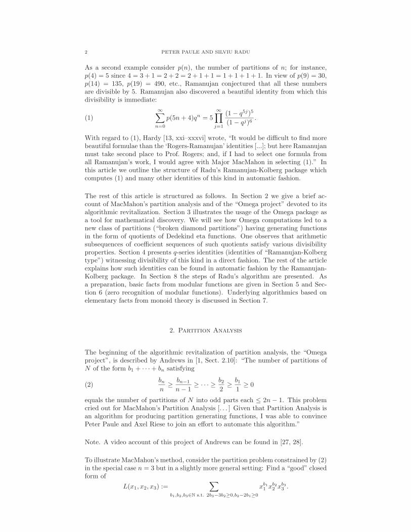
As a second example consider p(n), the number of partitions of n; for instance,p(4) = 5 since 4 = 3 + 1 = 2 + 2 = 2 + 1 + 1 = 1 + 1 + 1 + 1. In view of p(9) = 30,p(14) = 135, p(19) = 490, etc., Ramanujan conjectured that all these numbersare divisible by 5. Ramanujan also discovered a beautiful identity from which thisdivisibility is immediate:
(1)
∞∑
n=0
p(5n+ 4)qn = 5
∞∏
j=1
(1− q5j)5
(1− qj)6.
With regard to (1), Hardy [13, xxi–xxxvi] wrote, “It would be difficult to find morebeautiful formulae than the ‘Rogers-Ramanujan’ identities [...]; but here Ramanujanmust take second place to Prof. Rogers; and, if I had to select one formula fromall Ramanujan’s work, I would agree with Major MacMahon in selecting (1).” Inthis article we outline the structure of Radu’s Ramanujan-Kolberg package whichcomputes (1) and many other identities of this kind in automatic fashion.
The rest of this article is structured as follows. In Section 2 we give a brief ac-count of MacMahon’s partition analysis and of the “Omega project” devoted to itsalgorithmic revitalization. Section 3 illustrates the usage of the Omega package asa tool for mathematical discovery. We will see how Omega computations led to anew class of partitions (“broken diamond partitions”) having generating functionsin the form of quotients of Dedekind eta functions. One observes that arithmeticsubsequences of coefficient sequences of such quotients satisfy various divisibilityproperties. Section 4 presents q-series identities (identities of “Ramanujan-Kolbergtype”) witnessing divisibility of this kind in a direct fashion. The rest of the articleexplains how such identities can be found in automatic fashion by the Ramanujan-Kolberg package. In Section 8 the steps of Radu’s algorithm are presented. Asa preparation, basic facts from modular functions are given in Section 5 and Sec-tion 6 (zero recognition of modular functions). Underlying algorithmics based onelementary facts from monoid theory is discussed in Section 7.
2. Partition Analysis
The beginning of the algorithmic revitalization of partition analysis, the “Omegaproject”, is described by Andrews in [1, Sect. 2.10]: “The number of partitions ofN of the form b1 + · · ·+ bn satisfying
(2)bnn
≥bn−1
n− 1≥ · · · ≥
b22
≥b11
≥ 0
equals the number of partitions of N into odd parts each ≤ 2n − 1. This problemcried out for MacMahon’s Partition Analysis [. . . ] Given that Partition Analysis isan algorithm for producing partition generating functions, I was able to convincePeter Paule and Axel Riese to join an effort to automate this algorithm.”
Note. A video account of this project of Andrews can be found in [27, 28].
To illustrate MacMahon’s method, consider the partition problem constrained by (2)in the special case n = 3 but in a slightly more general setting: Find a “good” closedform of
L(x1, x2, x3) :=∑
b1,b2,b3∈N s.t. 2b3−3b2≥0,b2−2b1≥0
xb11 xb2
2 xb33 .
PARTITION ANALYSIS, MODULAR FUNCTIONS, AND COMPUTER ALGEBRA 3
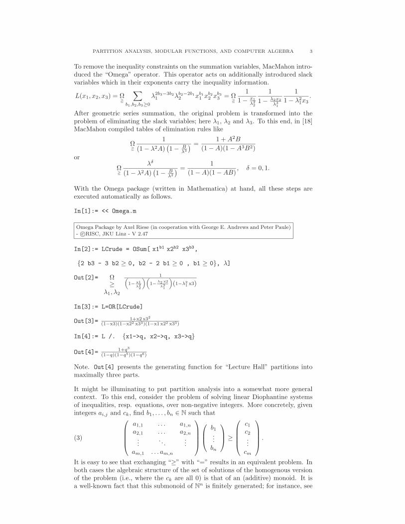
To remove the inequality constraints on the summation variables, MacMahon intro-duced the “Omega” operator. This operator acts on additionally introduced slackvariables which in their exponents carry the inequality information.
L(x1, x2, x3) = Ω≧
∑
b1,b2,b3≥0
λ2b3−3b21 λb2−2b1
2 xb11 xb2
2 xb33 = Ω
≧
1
1− x1
λ22
1
1− λ2x2
λ31
1
1− λ21x3
.
After geometric series summation, the original problem is transformed into theproblem of eliminating the slack variables; here λ1, λ2 and λ3. To this end, in [18]MacMahon compiled tables of elimination rules like
Ω≧
1
(1− λ2A)(
1− Bλ3
) =1 +A2B
(1−A)(1−A3B2)
or
Ω≧
λδ
(1− λ2A)(
1− Bλ2
) =1
(1−A)(1−AB), δ = 0, 1.
With the Omega package (written in Mathematica) at hand, all these steps areexecuted automatically as follows.
In[1]:= << Omega.m
Omega Package by Axel Riese (in cooperation with George E. Andrews and Peter Paule)- c©RISC, JKU Linz - V 2.47
In[2]:= LCrude = OSum[ x1b1 x2b2 x3b3,
2 b3 - 3 b2 ≥ 0, b2 - 2 b1 ≥ 0 , b1 ≥ 0, λ]
Out[2]= Ω≥
λ1, λ2
1(
1− x1
λ22
)(
1−λ2 x2
λ31
)
(1−λ21 x3)
In[3]:= L=OR[LCrude]
Out[3]= 1+x2 x32
(1−x3)(1−x22 x33)(1−x1 x22 x33)
In[4]:= L /. x1->q, x2->q, x3->q
Out[4]= 1+q3
(1−q)(1−q5)(1−q6)
Note. Out[4] presents the generating function for “Lecture Hall” partitions intomaximally three parts.
It might be illuminating to put partition analysis into a somewhat more generalcontext. To this end, consider the problem of solving linear Diophantine systemsof inequalities, resp. equations, over non-negative integers. More concretely, givenintegers ai,j and ck, find b1, . . . , bn ∈ N such that
(3)
a1,1 . . . a1,na2,1 . . . a2,n...
. . ....
am,1 . . . am,n
b1...bn
≥
c1c2...cm
.
It is easy to see that exchanging “≥” with “=” results in an equivalent problem. Inboth cases the algebraic structure of the set of solutions of the homogenous versionof the problem (i.e., where the ck are all 0) is that of an (additive) monoid. It isa well-known fact that this submonoid of Nn is finitely generated; for instance, see
4 PETER PAULE AND SILVIU RADU
the classical book by Grace and Young where this is proved as a consequence of aversion of the celebrated Hilbert Basis Theorem [12].
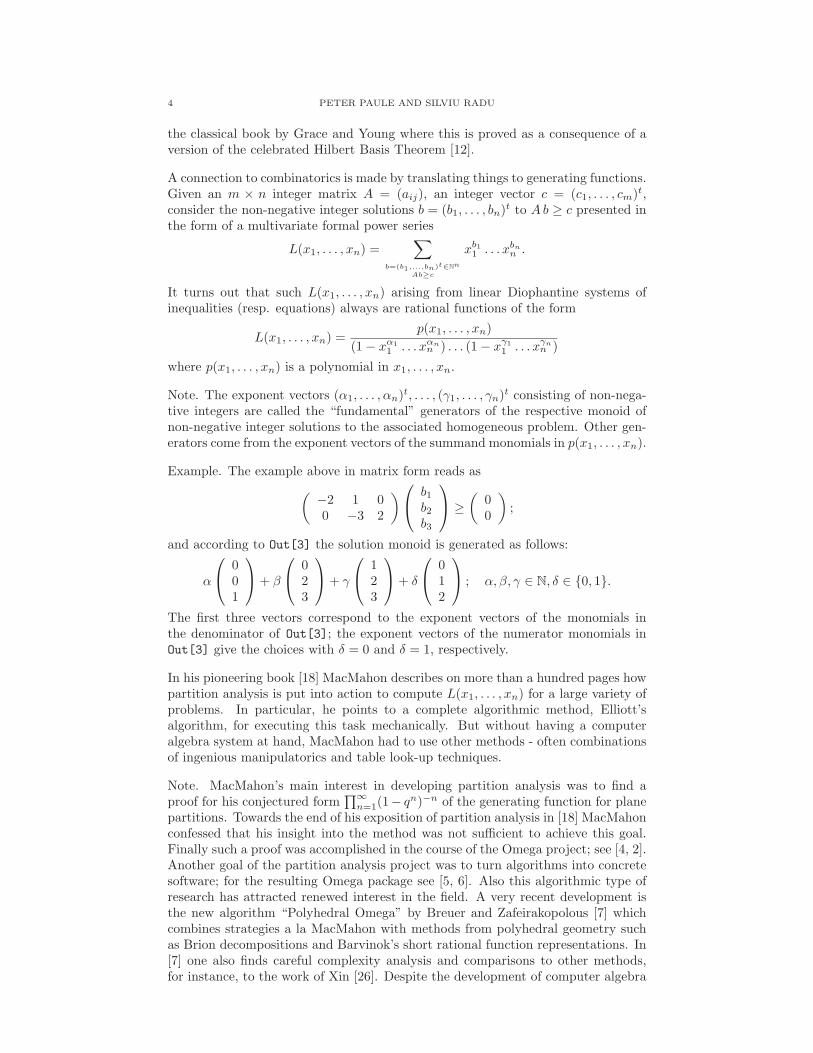
A connection to combinatorics is made by translating things to generating functions.Given an m × n integer matrix A = (aij), an integer vector c = (c1, . . . , cm)t,consider the non-negative integer solutions b = (b1, . . . , bn)
t to Ab ≥ c presented inthe form of a multivariate formal power series
L(x1, . . . , xn) =∑
b=(b1,...,bn)t∈Nn
Ab≥c
xb11 . . . xbn
n .
It turns out that such L(x1, . . . , xn) arising from linear Diophantine systems ofinequalities (resp. equations) always are rational functions of the form
L(x1, . . . , xn) =p(x1, . . . , xn)
(1− xα11 . . . xαn
n ) . . . (1− xγ1
1 . . . xγnn )
where p(x1, . . . , xn) is a polynomial in x1, . . . , xn.
Note. The exponent vectors (α1, . . . , αn)t, . . . , (γ1, . . . , γn)
t consisting of non-nega-tive integers are called the “fundamental” generators of the respective monoid ofnon-negative integer solutions to the associated homogeneous problem. Other gen-erators come from the exponent vectors of the summand monomials in p(x1, . . . , xn).
Example. The example above in matrix form reads as
(
−2 1 00 −3 2
)
b1b2b3
≥
(
00
)
;
and according to Out[3] the solution monoid is generated as follows:
α
001
+ β
023
+ γ
123
+ δ
012
; α, β, γ ∈ N, δ ∈ 0, 1.
The first three vectors correspond to the exponent vectors of the monomials inthe denominator of Out[3]; the exponent vectors of the numerator monomials inOut[3] give the choices with δ = 0 and δ = 1, respectively.
In his pioneering book [18] MacMahon describes on more than a hundred pages howpartition analysis is put into action to compute L(x1, . . . , xn) for a large variety ofproblems. In particular, he points to a complete algorithmic method, Elliott’salgorithm, for executing this task mechanically. But without having a computeralgebra system at hand, MacMahon had to use other methods - often combinationsof ingenious manipulatorics and table look-up techniques.
Note. MacMahon’s main interest in developing partition analysis was to find aproof for his conjectured form
∏∞n=1(1− qn)−n of the generating function for plane
partitions. Towards the end of his exposition of partition analysis in [18] MacMahonconfessed that his insight into the method was not sufficient to achieve this goal.Finally such a proof was accomplished in the course of the Omega project; see [4, 2].Another goal of the partition analysis project was to turn algorithms into concretesoftware; for the resulting Omega package see [5, 6]. Also this algorithmic type ofresearch has attracted renewed interest in the field. A very recent development isthe new algorithm “Polyhedral Omega” by Breuer and Zafeirakopolous [7] whichcombines strategies a la MacMahon with methods from polyhedral geometry suchas Brion decompositions and Barvinok’s short rational function representations. In[7] one also finds careful complexity analysis and comparisons to other methods,for instance, to the work of Xin [26]. Despite the development of computer algebra

PARTITION ANALYSIS, MODULAR FUNCTIONS, AND COMPUTER ALGEBRA 5
packages like Omega, the primary goal of the Omega project by Andrews, Paule,and Riese was not the improvement of computational complexity but the usage ofsuch packages in the process of mathematical discovery.
3. Omega and Mathematical Discovery
As already mentioned, MacMahon generalized partitions of numbers arranged “ona line” like 3 = 2 + 1 = 1 + 1 + 1, to plane partitions arranged “in the plane”, like
3, 2 + 1,2+1
, 1 + 1 + 1,
1+1+1
,1 + 1+1
.
Alternatively, plane partitions which, for example, are arranged in maximally tworows can be described by posets, respectively directed graphs, as follows:
a11 a12 a13
a22a21 a23
. . .
Here the aij represent non-negative integers following order conditions prescribedby the arrows. For instance, the arrow from a11 to a21 means a11 ≥ a21. Using theOmega package it is easy to compute corresponding partition generating functions.For example, consider the following poset:
P = a1
a2 a5 a8
a3 a6 a9
a4 a7 a10
andL(q) :=
∑
a1,...,a10≥0 s.t. P
qa1+···+a10 .
One computes the rational function presentation of L(q) just as in the Omegaexample above, and obtains
L(q) =1 + q8
(1− q)(1− q2)2(1− q3)(1− q5)2(1− q6)(1− q7)(1− q8)(1− q9).
Computational experiments with the Omega package led to replacing the poset Pby a k-elongated diamond of length 1:
a1
❯
a2
a3
❯
a4
a5
❯
a6. . . . . . . . . .
a7. . . . . . . . . .
a2k−1
❯
a2k−2
a2k+1
❯
a2k
a2k+2

6 PETER PAULE AND SILVIU RADU
More generally, one can glue n such diamonds together to obtain a k-elongatedpartition diamond of length n:
a1
❯
a2
. . . . . . . .
a3
. . . . . . . . a2k
a2k+1
❯a2k+2
❯
a2k+3
. . . . . . . .
a2k+4
. . . . . . . . a4k+1
a4k+2
❯a4k+3 . . . . . .
❯
. . . . . . . .
. . . . . . . . a(2k+1)n−1
a(2k+1)n
❯a(2k+1)n+1
In [3] it is shown that the generating function for k-elongated diamonds of lengthn is
hn,k(q) =
∏n−1j=0 (1 + q(2k+1)j+2)(1 + q(2k+1)j+4) . . . (1 + q(2k+1)j+2k)
∏(2k+1)n+1j=1 (1− qj)
.
But one does not need to stop here. Andrews ingeniously suggested to “delete thesource”; this means, to remove the a1-vertex together with its outgoing edges. Theresult is a surprise; namely, for the generating function h∗
n,k(q) over the resultingposet one obtains
h∗n,k(q) =
∏n−1j=0 (1 + q(2k+1)j+1)(1 + q(2k+1)j+3) . . . (1 + q(2k+1)j+2k−1)
∏(2k+1)nj=1 (1− qj)
.
This leads us to consider the poset which results after gluing these diamonds to-gether:
b(2k+1)n+1
b(2k+1)n−1
. . . . . . . .
b(2k+1)n
. . . . . . . .
. . .
. . . . . . . .
. . . . . . . .
b7
b6
b5
b4
b3
b2
b2k+2
b2k+1
b2k
a1
❯
a2
. . . . . . . .
a3
. . . . . . . . a2k
a2k+1
❯a2k+2 . . .
❯
. . . . . . . .
. . . . . . . . a(2k+1)n−1
a(2k+1)n
❯a(2k+1)n+1
Why considering this? In the limit n → ∞ the corresponding generating functionbecomes:
∞∑
m=0
∆k(m)qm := limn→∞
hn,k(q)h∗n,k(q)
=
∏∞j=1(1 + qj)
∏∞j=1(1− qj)2
∏∞j=1(1 + q(2k+1)j)
=
∏∞j=1(1 + qj)(1− qj)
∏∞j=1(1− qj)3
∏∞j=1(1 + q(2k+1)j)
=
∞∏
j=1
(1− q2j)(1− q(2k+1)j)
(1− qj)3(1− q(4k+2)j).
Consequently, we have constructed combinatorial objects whose generating functionis a non-trivial eta-quotient:
∞∑
m=0
∆k(m)qm = qk+112
η(2τ)η((2k + 1)τ)
η(τ)3η((4k + 2)τ)

PARTITION ANALYSIS, MODULAR FUNCTIONS, AND COMPUTER ALGEBRA 7
with η the Dedekind eta function defined as usual as
(4) η(τ) := q124
∞∏
n=1
(1− qn)
where q = e2πiτ for τ ∈ H, H := τ ∈ C : Im > 0 the upper half complex plane.Note that when presenting the generating function in terms of the Dedekind etafunction, we moved from viewing q as an indeterminate arising in a formal powerseries to q = q(τ) presenting a function in the complex plane. In the following wewill move freely between these two worlds; issues like convergence can be settledeasily in each individual case.
Most relevant for our context, q-series defined by quotients of η-functions oftenpossess remarkable number theoretic properties. Such properties can be studiedmost comfortably with the help of computer algebra systems.
For example, let us input a truncated product version of the generating functionfor k-elongated diamonds:
In[5]:= bd[N , k ] :=∏N
j=1(1−q2j)(1−q(2k+1)j)(1−qj)3(1−q(4k+2)j)
Already the case k = 1 will turn out to be interesting. We will inspect the coefficientsof the Taylor series expansion up to that of q30.
In[6]:= bd1 = Normal[Series[bd[30,1], q,0,30]]
Out[6]=1 + 3q + 8q2 + 18q3 + 38q4 + 75q5 + 142q6 + 258q7 + 455q8 + 780q9 + 1308q10
+ 2148q11 + 3467q12 + 5505q13 + 8168q14 + 13314q15 + 20327q16 + 30693q17
+ 45882q18 + 67944q19 + 99745q20 + 145239q21 + 209882q22 + 301128q23
+ 429148q24 + 607710q25 + 855414q26 + 1197228q27 + 1666585q28
+ 2308014q29 + 3180668q30
First we take all the coefficients modulo 2.
In[7]:= Mod[CoefficientList[bd1, q], 2]
Out[7]= 1, 1, 0, 0, 0, 1, 0, 0, 1, 0, 0, 0, 1, 1, 0, 0, 1, 1, 0,
0, 1, 1, 0, 0, 0, 0, 0, 0, 1, 0, 0
Next we take the coefficients modulo 3 and 4.
In[8]:= Mod[CoefficientList[bd1, q], 3]
Out[8]= 1, 0, 2, 0, 2, 0, 1, 0, 2, 0, 0, 0, 2, 0, 2, 0, 2, 0, 0,
0, 1, 0, 2, 0, 1, 0, 0, 0, 1, 0, 2
In[9]:= Mod[CoefficientList[bd1, q], 4]
Out[9]= 1, 3, 0, 2, 2, 3, 2, 2, 3, 0, 0, 0, 3, 1, 2, 2, 3, 1, 2,
0, 1, 3, 2, 0, 0, 2, 2, 0, 1, 2, 0
In contrast to the cases modulo 2 and modulo 4, a quick inspection suggests a clearpattern modulo 3:
(5) ∆1(2n+ 1) ≡ 0 (mod 3), n ∈ N.
8 PETER PAULE AND SILVIU RADU
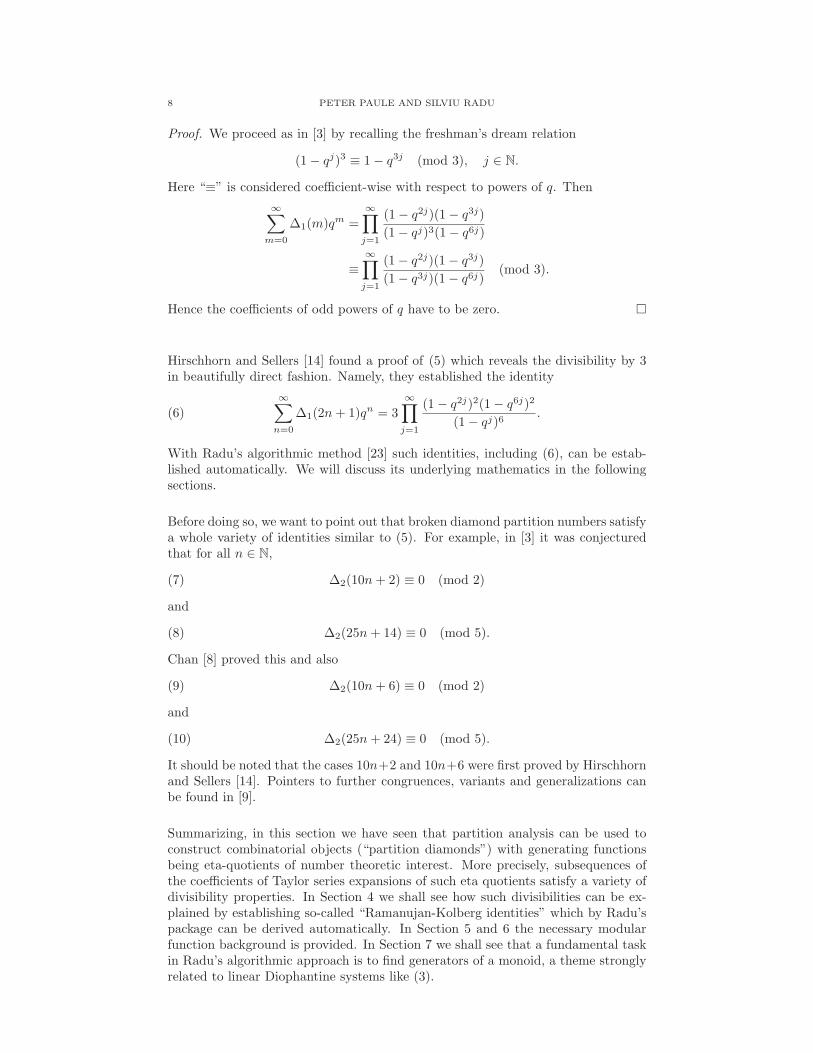
Proof. We proceed as in [3] by recalling the freshman’s dream relation
(1− qj)3 ≡ 1− q3j (mod 3), j ∈ N.
Here “≡” is considered coefficient-wise with respect to powers of q. Then
∞∑
m=0
∆1(m)qm =
∞∏
j=1
(1− q2j)(1− q3j)
(1− qj)3(1− q6j)
≡
∞∏
j=1
(1− q2j)(1− q3j)
(1− q3j)(1− q6j)(mod 3).
Hence the coefficients of odd powers of q have to be zero.
Hirschhorn and Sellers [14] found a proof of (5) which reveals the divisibility by 3in beautifully direct fashion. Namely, they established the identity
(6)
∞∑
n=0
∆1(2n+ 1)qn = 3
∞∏
j=1
(1− q2j)2(1− q6j)2
(1− qj)6.
With Radu’s algorithmic method [23] such identities, including (6), can be estab-lished automatically. We will discuss its underlying mathematics in the followingsections.
Before doing so, we want to point out that broken diamond partition numbers satisfya whole variety of identities similar to (5). For example, in [3] it was conjecturedthat for all n ∈ N,
(7) ∆2(10n+ 2) ≡ 0 (mod 2)
and
(8) ∆2(25n+ 14) ≡ 0 (mod 5).
Chan [8] proved this and also
(9) ∆2(10n+ 6) ≡ 0 (mod 2)
and
(10) ∆2(25n+ 24) ≡ 0 (mod 5).
It should be noted that the cases 10n+2 and 10n+6 were first proved by Hirschhornand Sellers [14]. Pointers to further congruences, variants and generalizations canbe found in [9].
Summarizing, in this section we have seen that partition analysis can be used toconstruct combinatorial objects (“partition diamonds”) with generating functionsbeing eta-quotients of number theoretic interest. More precisely, subsequences ofthe coefficients of Taylor series expansions of such eta quotients satisfy a variety ofdivisibility properties. In Section 4 we shall see how such divisibilities can be ex-plained by establishing so-called “Ramanujan-Kolberg identities” which by Radu’spackage can be derived automatically. In Section 5 and 6 the necessary modularfunction background is provided. In Section 7 we shall see that a fundamental taskin Radu’s algorithmic approach is to find generators of a monoid, a theme stronglyrelated to linear Diophantine systems like (3).
PARTITION ANALYSIS, MODULAR FUNCTIONS, AND COMPUTER ALGEBRA 9
4. Ramanujan-Kolberg Identities
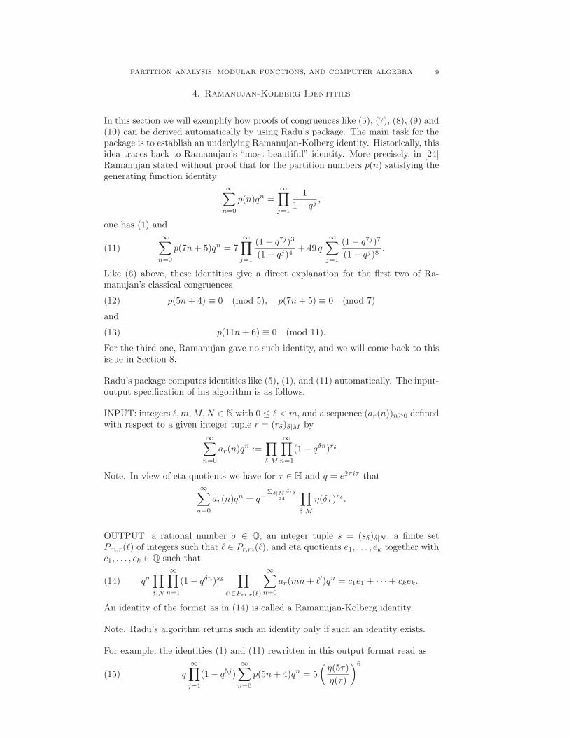
In this section we will exemplify how proofs of congruences like (5), (7), (8), (9) and(10) can be derived automatically by using Radu’s package. The main task for thepackage is to establish an underlying Ramanujan-Kolberg identity. Historically, thisidea traces back to Ramanujan’s “most beautiful” identity. More precisely, in [24]Ramanujan stated without proof that for the partition numbers p(n) satisfying thegenerating function identity
∞∑
n=0
p(n)qn =∞∏
j=1
1
1− qj,
one has (1) and
(11)
∞∑
n=0
p(7n+ 5)qn = 7
∞∏
j=1
(1− q7j)3
(1− qj)4+ 49 q
∞∑
j=1
(1− q7j)7
(1− qj)8.
Like (6) above, these identities give a direct explanation for the first two of Ra-manujan’s classical congruences
(12) p(5n+ 4) ≡ 0 (mod 5), p(7n+ 5) ≡ 0 (mod 7)
and
(13) p(11n+ 6) ≡ 0 (mod 11).
For the third one, Ramanujan gave no such identity, and we will come back to thisissue in Section 8.
Radu’s package computes identities like (5), (1), and (11) automatically. The input-output specification of his algorithm is as follows.
INPUT: integers ℓ,m,M,N ∈ N with 0 ≤ ℓ < m, and a sequence (ar(n))n≥0 definedwith respect to a given integer tuple r = (rδ)δ|M by
∞∑
n=0
ar(n)qn :=
∏
δ|M
∞∏
n=1
(1− qδn)rδ .
Note. In view of eta-quotients we have for τ ∈ H and q = e2πiτ that∞∑
n=0
ar(n)qn = q−
∑
δ|M δrδ24
∏
δ|M
η(δτ)rδ .
OUTPUT: a rational number σ ∈ Q, an integer tuple s = (sδ)δ|N , a finite setPm,r(ℓ) of integers such that ℓ ∈ Pr,m(ℓ), and eta quotients e1, . . . , ek together withc1, . . . , ck ∈ Q such that
(14) qσ∏
δ|N
∞∏
n=1
(1− qδn)sδ∏
ℓ′∈Pm,r(ℓ)
∞∑
n=0
ar(mn+ ℓ′)qn = c1e1 + · · ·+ ckek.
An identity of the format as in (14) is called a Ramanujan-Kolberg identity.
Note. Radu’s algorithm returns such an identity only if such an identity exists.
For example, the identities (1) and (11) rewritten in this output format read as
(15) q∞∏
j=1
(1− q5j)∞∑
n=0
p(5n+ 4)qn = 5
(
η(5τ)
η(τ)
)6

10 PETER PAULE AND SILVIU RADU
and
(16) q∞∏
j=1
(1− q7j)∞∑
n=0
p(7n+ 5)qn = 7
(
η(7τ)
η(τ)
)4
+ 49
(
η(7τ)
η(τ)
)8
,
respectively. In both cases Pm,r(ℓ) = ℓ with ℓ = 4 and ℓ = 5, respectively.
Note. Identities of the form (14) where Pm,r(ℓ) is bigger than ℓ go back toKolberg [16].
To give a concrete example in the context of broken partition diamonds, recall thecongruences (8) and (10):
(17) ∆2(25n+ 14) ≡ ∆2(25n+ 24) ≡ 0 (mod 5), n ∈ N.
Using (1− qj)5 ≡ 1− q5j (mod 5) we observe that
∞∑
m=0
∆2(n)qn =
∞∏
j=1
(1− q2j)(1− q5j)
(1− qj)3(1− q10j)≡
∞∏
j=1
(1− q2j)(1− qj)2
(1− q10j)(mod 5)
=:∞∑
n=0
d(n)qn.
Hence ∆2(n) ≡ d(n) (mod 5), and we will prove (17) with d(n) instead of ∆2(n).
Radu’s program “Ramanujan-Kolberg” delivers
q32η(2τ)12η(5τ)10
η(τ)6η(10τ)20
(
∞∑
m=0
d(25n+ 14)qn
)(
∞∑
m=0
d(25n+ 24)qn
)
=25(2t4 + 28t3 + 155t2 + 400t+ 400)
(18)
where
(19) t =η(τ)3η(5τ)
η(2τ)η(10τ)3.
Rewriting the η-quotients in terms of q-products of the form
∞∏
k=1
(1− qδk)tk
makes the divisibility by 5 for each of the two classes d(25n+ 14) and d(25n+ 24)explicit.
Here, in view of (14), ℓ = 14, m = 25, M = N = 10, r = (r1, r2, r5, r10) =(2, 1, 0,−1), s = (s1, s2, s5, s10) = (−6, 12, 10,−20), σ = −4 and Pm,r(ℓ) = 14, 24.
Note. The program computes a similar identity also for ∆2(n) instead of d(n), butthe output is much bigger.
For the automatic derivation of Ramanujan-Kolberg identities of the form (14)Radu has chosen a particular setting in order to deal with modular functions in analgebraic fashion. The basic ingredients to this setting are given in the Sections 5,6, and 7. The description of the steps of Radu’s Ramanujan-Kolberg Algorithm canbe found in Section 8.
PARTITION ANALYSIS, MODULAR FUNCTIONS, AND COMPUTER ALGEBRA 11
5. Modular Functions: Basic Notions
As defined by (4) at the end of Section 3, eta functions are holomorphic functionsdefined on the upper half of the complex plane. Obviously, for f(τ) := η(τ)24 wehave the periodicity f(τ + 1) = f(τ) for τ ∈ H.
Note. In view of q-series representation we recall a fundamental, but importantfact. Namely, for a given holomorphic function f(τ) on H with period N ∈ N \ 0(i.e., f(τ +N) = f(τ), τ ∈ H), there exists (uniquely) a holomorphic function h(τ)on the open unit disk, punctured at 0, such that for all τ ∈ H:
(20) f(τ) = h(e2πiτ/N ).
For example, for f(τ) := η(τ)24 (i.e., N = 1) one has
h(q) = q
(
∞∑
n=1
p(n)qn
)−24
for all q from the punctured open unit disc.
But more is true. Namely, f(τ) := η(τ)24 satisfies
(21) f
(
aτ + b
cτ + d
)
= (cτ + d)kf(τ), τ ∈ H,
for k = 12 and all
(
a bc d
)
∈ SL2(Z) =
(
a bc d
)
∈ Z2×2 : ad− bc = 1
. Holo-
morphic functions on H with this property plus suitable asymptotic behaviour atτ ∈ Q ∪ ∞ are called modular forms of weight k for SL2(Z).
Note. A standard reference for modular forms and the related arithmetic of theirq-series coefficients is [20].
Taking quotients g(τ) := f1(τ)/f2(τ) of such modular forms f1(τ) and f2(τ) resultin stronger symmetry:
(22) g
(
aτ + b
cτ + d
)
= g(τ),
(
a bc d
)
∈ SL2(Z), τ ∈ H.
Note:(
a bc d
)
(τ) :=aτ + b
cτ + d
defines a group action of SL2(Z) on H. Often one writes γτ instead of γ(τ) whereγ ∈ SL2(Z).
Sometimes one needs to restrict property (22) to
(
a bc d
)
from subgroups of
SL2(Z), for instance,
(
a bc d
)
∈ Γ0(N), N ∈ N \ 0, where
Γ0(N) :=
(
a bc d
)
∈ SL2(Z) : N |c
.
Modular forms g of weight k = 0 with symmetry (22) for
(
a bc d
)
∈ Γ0(N)
(i.e., (23) below) and being holomorphic on H are called modular functions forΓ0(N). It is obvious that such functions for fixed N form C-algebras; i.e., they arecommutative rings with 1 and vector spaces over C.
Notation. The C-algebra of modular functions for Γ0(N) will be denoted by M(N).

12 PETER PAULE AND SILVIU RADU
For example, one can show that the functions (η(5τ)/η(τ))6 from (15), and f(z)and f(z)2 with f(z) = (η(7τ)/η(τ))4 from (16) are elements from M(5) and M(7),respectively. To this end, one needs to verify for N = 5, resp N = 7 the followingvariant of (22) :
(23) g
(
aτ + b
cτ + d
)
= g(τ),
(
a bc d
)
∈ Γ0(N), τ ∈ H,
and the suitable asymptotic behaviour at all τ ∈ Q∪∞. This “suitable asymptoticbehaviour” is described by using the Laurent expansion as in (20) of h around 0.Consider τ ∈ H close to ∞ or to a point a
c ∈ Q. Allowing c = 0 we include the case
∞ = a0 . For γ =
(
a bc d
)
∈ SL2(Z) we have γ(∞) = ac . Because of periodicity
the following theorem holds [15, Thm 4].
Theorem 5.1. Let γ(∞) = ac for γ =
(
a bc d
)
∈ Γ0(N) and g be a holomorphic
function on H satisfying (23). Then for all τ ∈ H sufficiently close to ac ∈ Q∪∞
there exists a Laurent series expansion such that
(24) g(τ) =
∞∑
n=−∞
cn(γ)e2πin(γ−1τ)/wγ
where
wγ := min
h ∈ N∗ :
(
1 h0 1
)
∈ γ−1Γ0(N)γ
.
Now we can give a precise definition of modularity. Namely, g as in the theorem iscalled a modular function, if (23) holds, and if
(25) for all γ ∈ SL2(Z) : cn(γ) = 0 for almost all negative n.
(Instead of (25) one also says that g is meromorphic at τ = ac = γ∞.) If this holds
and if m is the smallest index such that cm(γ) 6= 0, then we call m the γ-order of gat τ = a
c ; notation: m = ordγa/c(g).
Note. If cn(γ) = 0 for all n ∈ Z we set ordγa/c(g) = ∞.
Using the fact that γ−12 γ1∞ = ∞ iff γ−1
2 γ1 =
(
1 h0 1
)
for some k ∈ Z, it is not
too difficult to check that if ac = γ1∞ = γ2∞ for γ1, γ2 ∈ SL2(Z), then wγ1
= wγ2
and
(26) ordγ1
a/c(g) = ordγ2
a/c(g).
Thus we can define the order of a modular function g at ac ∈ Q ∪ ∞ by
orda/c(g) := ordγa/c(g)
for some γ ∈ SL2(Z) such that γ∞ = ac .
On the same line, let g be a modular function, and let γ∞ = ac ∈ Q ∪ ∞ for
γ =
(
a bc d
)
∈ SL2(Z) with expansion at ac being
g(τ) =∑
n≥orda/c
cn(γ)e2πi(γ−1τ)/wγ .
Furthermore, let γ′ =
(
a′ b′
c′ d′
)
∈ SL2(Z) be such that γ′ = γ0γ for some γ0 ∈
Γ0(N). Thenwγ′ = wγ
PARTITION ANALYSIS, MODULAR FUNCTIONS, AND COMPUTER ALGEBRA 13
owing to (γ′)−1Γ0(N)γ′ = γ−1Γ0(N)γ. In addition, g has an expansion at a′
c′ = γ′∞as follows
g(τ) =∑
n≥orda′/c′ (g)
cn(γ′)e2πi((γ
′)−1τ)/wγ′
=∑
n≥orda′/c′ (g)
cn(γ′)e2πi(γ
−1τ)/wγ
where the second equality is by g(τ) = g(γ0τ). Hence, by uniqueness of Laurentexpansion, for all n ∈ Z:
(27) cn(γ′) = cn(γ); in particular , ordγ
′
a′/c′(g) = ordγa/c(g).
In other words, the (24) expansions at points a′
c′ = γ0ac with γ0 ∈ Γ0(N) are all the
same.
Example. For g(τ) := (η(5τ)/η(τ))6 property (23) for N = 5 follows from a refinedversion of the symmetry (21) for the η-function. To show property (25) we needto show that for all γ ∈ SL2(Z) the expansion (24) has only a finite sum as itsprincipal part. In view of property (27), this task can be reduced to a finite numberof inspections. To this end, we make use of the coset decomposition [15].
(28) SL2(Z) = Γ0(5) ∪ Γ0(5)T ∪ Γ0(5)TS ∪ · · · ∪ Γ0(5)TS4
where
S =
(
1 10 1
)
, and T =
(
0 −11 0
)
;
this means, we just need to check for γ = id, T, TS, . . . , TS4.
A further reduction of the number of inspections comes from the fact that S(∞) =∞ and thus
id(∞) = ∞ and TSj(∞) = 0 (j = 0, . . . , 4).
This means, we need to inspect the Laurent expansion (24) for all τ close to ∞ (i.e.,choosing γ = id) and close to 0 (i.e., for γ = T ). For γ = id we can invoke (4) withq = e2πiτ
g(τ) = q
∞∏
j=1
(
1− q5j
1− qj
)6
;
i.e., ord∞(g) = 1. For γ = T we have to use [15, Thm. 9]
(29) η(
−1
τ
)
= (−i)1/2τ1/2η(τ), τ ∈ H,
(taking that branch of the square root function τ1/2 which is positive for real τ > 0)and obtain for τ close to 0:
(30) g(τ) =1
531
Q
∞∏
j=1
( 1−Qj
1−Q5j
)6
where Q = e2πi(T−1τ)/5. This means, ord0(g) = −1.
Note 1. Relation (30) corresponds to the following relation:
g(τ)g(
−1
5τ
)
=1
53, τ ∈ H.
Note 2. Matching the right hand side of (30) to the series expansion as in (24) onesees that wT = 5. This is in accordance with the fact [17, Lemma 3.2.4]
(31) wγ =N
gcd(c2, N)if γ =
(
a bc d
)
∈ Γ0(N).

14 PETER PAULE AND SILVIU RADU
Summarizing, with these considerations we have sharpened our understanding ofmodular functions for a given group Γ0(N). Recall that these objects form a C-algebra which we denoted by M(N). We also note that if f(τ) ∈ M(N) withouthaving roots in the upper half complex plane, then also
1
f(τ)∈ M(N).
6. Modular Functions: Zero Recognition
Our task is to establish and to prove algebraic relations between functions fromM(N). To illustrate various points, consider the following functions on H usingq = e2πiτ :
(32) f(τ) := q
∞∏
j=1
(1− q5j)
∞∑
n=0
p(5n+ 4)qn
and
(33) g(τ) := q
∞∏
j=1
(
1− q5j
1− qj
)6
=
(
η(5τ)
η(τ)
)6
.
Following the example above we know that g ∈ M(5). Suppose we also know thatf ∈ M(5). Equipped with this knowledge: how does one prove (15); i.e.,
(34) f(τ)− 5g(τ) = 0, τ ∈ H?
Since both functions can be expressed as power series in q, one way to proceedwould be comparing the (infinitely) many coefficients in these expansions. However,in the given context, it is non-trivial to turn this strategy into a feasible (finitary)argument. Rather than that, one looks at expansions at points a
c ∈ Q∪∞, wherepoles arise. In view of (24), the representations in (32) and (33) correspond to
expansions at γ∞ = 10 = ∞ with γ =
(
1 00 1
)
and where w∞ = 1 by (31). Next
consider the expansion at γ∞ = 01 = 0 with γ =
(
0 −11 0
)
= T and w0 = 5
by (31). If we expand (30) in powers of Q = e2πi(T−1τ)/5 we obtain
g(τ) =1
53Q−1 −
6
53+
9
53Q1 + . . . .
As we shall see below, to prove (15) it is sufficient to check for the Q-expansion
f(τ) =
∞∑
n=−∞
cn(T )Qn,
whether ord0(f) = −1 and whether
(35) c−1(T ) =1
52and c0 = −
6
52.
This is done as follows. First, rewrite f(τ), as defined in (32) as
f(τ) = q1924 η(5τ)
∞∑
n=0
p(5n+ 4)qn
and define
H(τ) :=1
5η(5τ) and F (τ) := 5q
1924
∞∑
n=0
p(5n+ 4)qn.

PARTITION ANALYSIS, MODULAR FUNCTIONS, AND COMPUTER ALGEBRA 15
By (29) we have
H(Tτ) =1
5(−i)1/2
(τ
5
)1/2
(q15 )24
∞∏
j=1
(1− (q15 )j).
To express F (Tτ) in terms of powers of q15 is more involved. Using properties of
the eta function, Rademacher [22] derived that
F (Tτ) =
4∑
λ=0
η(τ + 24λ
5
)−1
=(−i)−1/2(5τ)−1/2(q15 )−
2524
×
(
∞∏
n=1
(
1− (q15 )25n
)−1
− 5
∞∑
n=1
(n
5
)
p(n− 1)(q15 )n
)
(36)
where(
n5
)
is the Legendre symbol. Consequently,
f(τ) =f(T (T−1τ)) = H(T (T−1τ))F (T (T−1τ))
=1
52Q−1
∞∏
j=1
(1−Qj)
=×(
∞∑
n=0
p(n)Q25n − 5
∞∑
n=1
(n
5
)
p(n− 1)Qn)
=1
52Q−1 −
6
52+
9
52Q+ . . . ,
which confirms (35). Why is this sufficient to prove (34)?
Recall the following classical fact from complex analysis:
Theorem 6.1 (MMT). Let f be a holomorphic function on a connected open subsetU ⊆ C. Suppose there is a point p ∈ U such that |f(z)| ≤ |f(p)| for all z ∈ U . Thenf is constant on U .
This theorem (“Maximum Modulus Theorem”) generalizes word by word replacingC by a connected Riemann surface X; see [19, Thm. 1.36]. As a corollary oneobtains a fundamental tool for zero testing of modular functions:
Theorem 6.2 (ZT). Let f be a holomorphic function on a compact Riemann sur-face X. Then f is a constant function.
Proof. The function |f | is continuous on the compact space X, hence taking on amaximum at some point in X. Consequently, the Riemann surface version of theMMT implies that f is a constant function.
Note. Taking U = C in MMT gives Liouville’s theorem. In view of ZT this wouldcorrespond to choosing the Riemann sphere for X.
Where in our context is the compact Riemann surface X to apply theorem ZT forzero-testing of modular functions?
To answer this question we extend our group action from H to H := H ∪Q ∪ ∞:
Γ0(N)×H → H,((
a bc d
)
, τ
)
7→
(
a bc d
)
τ :=aτ + b
cτ + d.
16 PETER PAULE AND SILVIU RADU
Notation. We write [τ ] := γτ : γ ∈ Γ0(N) for τ -orbits and X0(N) for the set ofall orbits.
We remark that orbits of τ ∈ Q ∪ ∞ contain only elements from Q ∪ ∞. Thus
X0(N) = [τ ] : τ ∈ H ∪ [τ ] : τ ∈ Q ∪ ∞
as a disjoint union of orbit sets.
Note. There are only finitely many orbits in [τ ] : τ ∈ Q ∪ ∞. These orbits arecalled cusps of X0(N); the underlying geometrical motivation and the connection toRiemann surfaces can be found in books like [10]. Sometimes, by abuse of language,also a representative τ of a cusp [τ ] is called cusp.
Example. For N = 5 we determine [τ ] : τ ∈ Q ∪ ∞: Either τ = ac = 1
0 = ∞ or
τ = ac for relatively prime integers a and c. In any case there exists γ =
(
a bc d
)
∈
SL2(Z) such that γ∞ = ac . According to (28), γ ∈ Γ0(5) or γ = γ0TS
j with
γ0 ∈ Γ0(5) and j ∈ 0, . . . , 4. In the first case[
ac
]
= [∞], in the second case[
ac
]
= [0] because of TSj∞ = 0. Hence
X0(5) = [τ ] : τ ∈ H ∪ [0], [∞].
Modular functions on H can be turned into meromorphic functions on X0(N) asfollows: Suppose f ∈ M(N). For τ ∈ N define
f([τ ]) := f(τ).
Because of (23) this is well defined. For ac ∈ Q ∪ ∞ let γ∞ = a
c with γ =(
a bc d
)
∈ SL2(Z). Consider the Laurent expansion as in (24) for τ ∈ H close
to ac :
f(τ) =
∞∑
n=orda/c(f)
cn(γ)e2πin(γ−1τ)/wγ
with wγ = Ngcd(c2,N) as in (31). If now orda/c(f) < 0, define
f([a
c
])
:= ∞.
If orda/c = 0, define
f([a
c
])
:= c0(γ);
if orda/c(f) > 0, define
f([a
c
])
:= 0.
Because of (27) all these function values at ac ∈ Q ∪ ∞ are well-defined. Con-
sequently, with the definitions above any f ∈ M(N) gives rise to a function f onX0(N).
Without going into detail, the set of orbits X0(N) can be equipped with a (natural)topology to make it a compact Hausdorff space. In addition, by introducing suitablecharts (local homeomorphisms from X0(N) to C) X0(N) can be turned into aRiemann surface.
Therefore, modular functions f ∈ M(N) can be viewed as functions f on thecompact Riemann surface X0(N). One can check in a straight-forward fashion
that the functions f are meromorphic functions on X0(N) which, owing to f being

PARTITION ANALYSIS, MODULAR FUNCTIONS, AND COMPUTER ALGEBRA 17
holomorphic on H, have possible poles only at the cusps; i.e., at the points[
ac
]
withac ∈ Q ∪ ∞.
As concrete representations at these cusps, one has that for all τ ∈ H from a suitably
chosen open neighbourhood of ac = γ∞ ∈ Q ∪ ∞ with γ =
(
a bc d
)
∈ SL2(Z):
f([τ ]) = f(τ) =
∞∑
n=orda/c
cn(γ)e2πi(γ−1τ)/wγ .
Note. As “suitable neighbourhoods” of ac for a
c ∈ Q one can take open discs in H
which are tangent to the real axis and to which ac is adjoined; for a
c = ∞ one canchoose the “degenerated discs” τ ∈ H : Im(τ) > c, c ≥ 0.
If orda/c ≥ 0 for all cusps[
ac
]
then f is holomorphic and, by Theorem ZT, f is
even a constant function on X0(N).
As an obvious consequence, f is constant function on H. And as another obviousconsequence we obtain the following zero test for a modular function f ∈ M(N):
MF-ZeroTest.
(T1) Determine all different cusps [
ac
]
: ac ∈ Q ∪ ∞.
(T2) For each cusp representative ac = γ∞ with γ =
(
a bc d
)
∈ SL2(Z) deter-
mine whether all the coefficients of the principal part
−1∑
n=orda/c(f)
cn(γ)e2πi(γ−1τ)/wγ
are zero.
(T3) If the answer to (T2) in each instance is yes: choose a suitable cusp[
ac
]
to
test whether c0(γ) = 0.
7. Interlude: Monoids and Modular Functions
Before describing the Ramanujan-Kolberg Algorithm in Section 8, we have to intro-duce a special C-algebra of modular functions. This algebra and a related (commu-tative) monoid structure allow to simplify the MF-ZeroTest and to carry out alsoother algebraic/algorithmic tasks.
To this end, we consider those functions f ∈ M(N) for which f as a meromorphicfunction on X0(N) has a pole only at the cusp
[
ac
]
= [∞]; i.e.,
M∞(N) := f ∈ M(N) : orda/c(f) ≥ 0 for alla
c∈ Q.
As its ambient space M(N), also M∞(N) forms a C-algebra which, in addition,gives rise to a naturally defined additive monoid induced by the pole orders.
The natural numbers N = 0, 1, . . . form a commutative monoid with respect toboth multiplication (with identity element 1) and addition (with identity element 0).Let M ⊆ N be an additive submonoid. It is easily seen that M is finitely generated.Namely, fix some m ∈ M \0 and consider in M the equivalence classes modulo m.If a, a′ ∈ M such that a′ = a + ℓm for some ℓ ∈ N, then a′ can be discarded as
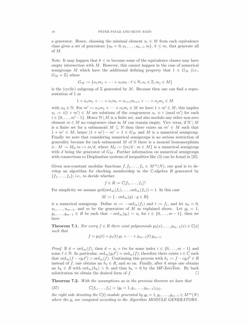
18 PETER PAULE AND SILVIU RADU
a generator. Hence, choosing the minimal element ui ∈ M from each equivalenceclass gives a set of generators u0 = 0, u1, . . . , uk−1,m, k ≤ m, that generate allof M .
Note. It may happen that k < m because some of the equivalence classes may haveempty intersection with M . However, this cannot happen in the case of numericalsemigroups M which have the additional defining property that 1 ∈ GM (i.e.,GM = Z) where
GM := α1m1 + · · ·+ αℓmℓ : ℓ ∈ N, αi ∈ Z,mj ∈ M
is the (cyclic) subgroup of Z generated by M . Because then one can find a repre-sentation of 1 as
1 + α1m1 + · · ·+ αimi = αi+1mi+1 + · · ·+ αjmj ∈ M
with αk ∈ N. For m′ := α1m1 + · · ·+ αimi ∈ M we have 1 +m′ ∈ M ; this impliesui := i(1 + m′) ∈ M are solutions of the congruences ui ≡ i (mod m′) for eachi ∈ 0, . . . ,m′−1. Hence N\M is a finite set, and also modulo any other non-zeroelement m ∈ M no congruence class in M can remain empty. Vice versa, if N \Mis a finite set for a submonoid M ⊆ N then there exists an m′ ∈ M such that1 + m′ ∈ M ; hence (1 + m′) − m′ = 1 ∈ GM and M is a numerical semigroup.Finally we note that considering numerical semigroups is no serious restriction ofgenerality because for each submonoid M of N there is a monoid homomorphismφ : M → Md,m 7→ m/d, where Md := m/d : m ∈ M is a numerical semigroupwith d being the generator of GM . Further information on numerical semigroupswith connections to Diophantine systems of inequalities like (3) can be found in [25].
Given non-constant modular functions f, f1, . . . , fn ∈ M∞(N), our goal is to de-velop an algorithm for checking membership in the C-algebra R generated byf1, . . . , fn; i.e., to decide whether
f ∈ R := C[f1, . . . , fn]?
For simplicity we assume gcd(ord∞(f1), . . . , ord∞(fn)) = 1. In this case
M := − ord∞(g) : g ∈ R
is a numerical semigroup. Define m := − ord∞(f1) and t := f1, and let u0 = 0,u1, . . . , um−1, and m be the generators of M as explained above. Let g0 = 1,g1, . . . , gm−1 ∈ R be such that − ord∞(gi) = ui for i ∈ 0, . . . ,m− 1, then wehave
Theorem 7.1. For every f ∈ R there exist polynomials p0(x), . . . , pm−1(x) ∈ C[x]such that
f = p0(t) + p1(t) g1 + · · ·+ pm−1(t) gm−1.
Proof. If d = ord∞(f), then d = ui + ℓm for some index i ∈ 0, . . . ,m − 1 andsome ℓ ∈ N. In particular, ord∞(git
ℓ) = ord∞(f); therefore there exists c ∈ C suchthat ord∞(f − cgit
ℓ) > ord∞(f). Continuing this process with h1 := f − cgitℓ ∈ R
instead of f , one obtains an h2 ∈ R, and so on. Finally, after k steps one obtainsan hk ∈ R with ord∞(hk) > 0, and thus hk = 0 by the MF-ZeroTest. By backsubstitution we obtain the desired form of f .
Theorem 7.2. With the assumptions as in the previous theorem we have that
(37) C[f1, . . . , fn] = 〈g0 = 1, g1, . . . , gm−1〉C[t],
the right side denoting the C[t]-module generated by g0 = 1, g1, . . . , gm−1 ∈ M∞(N)where the gi are computed according to the Algorithm MODULE GENERATORS.
PARTITION ANALYSIS, MODULAR FUNCTIONS, AND COMPUTER ALGEBRA 19
Proof. The following algorithm description shows how to obtain g1, . . . , gm−1 fromf1, . . . , fn in an algorithmic fashion. The rest of the statement is only a reformula-tion of Theorem 7.1.
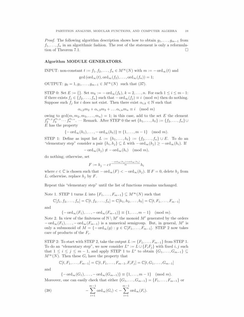
Algorithm MODULE GENERATORS.
INPUT: non-constant t := f1, f2, . . . , fn ∈ M∞(N) with m := − ord∞(t) and
gcd (ord∞(t), ord∞(f2), . . . , ord∞(fn)) = 1;
OUTPUT: g0 = 1, g1, . . . , gm−1 ∈ M∞(N) such that (37).
STEP 0: Set E := . Set mk := − ord∞(fk), k = 2, . . . , n. For each 1 ≤ i ≤ m−1:if there exists fj ∈ f2, . . . , fn such that − ord∞(fj) ≡ i (mod m) then do nothing.Suppose such fj for i does not exist. Then there exist αi,k ∈ N such that
αi,2m2 + αi,3m3 + . . . αi,nmn ≡ i (mod m)
owing to gcd(m,m2,m3, . . . ,mn) = 1; in this case, add to the set E the elementfαi,2
2 fαi,3
3 · · · fαi,nn . — Remark. After STEP 0 the set h1, . . . , hℓ := f2, . . . , fn∪
E has the property
− ord∞(h1), . . . ,− ord∞(hℓ) ≡ 1, . . . ,m− 1 (mod m).
STEP 1: Define as input list L := h1, . . . , hℓ := f2, . . . , fn ∪ E. To do an“elementary step” consider a pair hi, hj ⊆ L with − ord∞(hj) ≥ − ord∞(hi). If
− ord∞(hj) 6≡ − ord∞(hi) (mod m),
do nothing; otherwise, set
F := hj − c t− ord∞(hj)+ord∞(hi)
m hi
where c ∈ C is chosen such that − ord∞(F ) < − ord∞(hj). If F = 0, delete hj fromL; otherwise, replace hj by F .
Repeat this “elementary step” until the list of functions remains unchanged.
Note 1. STEP 1 turns L into F1, . . . , Fm−1 ⊆ M∞(N) such that
C[f1, f2, . . . , fn] = C[t, f2, . . . , fn] = C[h1, h2, . . . , hℓ] = C[t, F1, . . . , Fm−1]
and− ord∞(F1), . . . ,− ord∞(Fm−1) ≡ 1, . . . ,m− 1 (mod m).
Note 2. In view of the finiteness of N \M ′ the monoid M ′ generated by the orders− ord∞(F1), . . . ,− ord∞(Fm−1) is a numerical semigroup. But, in general, M ′ isonly a submonoid of M = − ord∞(g) : g ∈ C[F1, . . . , Fm−1]. STEP 2 now takescare of products of the Fi.
STEP 2: To start with STEP 2, take the output L := F1, . . . , Fm−1 from STEP 1.To do an “elementary step”, we now consider L∗ := L∪ FiFj with fixed i, j suchthat 1 ≤ i ≤ j ≤ m − 1, and apply STEP 1 to L∗ to obtain G1, . . . , Gm−1 ⊆M∞(N). Then these Gi have the property that
C[t, F1, . . . , Fm−1] = C[t, F1, . . . , Fm−1, FiFj ] = C[t, G1, . . . , Gm−1]
and− ord∞(G1), . . . ,− ord∞(Gm−1) ≡ 1, . . . ,m− 1 (mod m).
Moreover, one can easily check that either G1, . . . , Gm−1 = F1, . . . , Fm−1 or
(38) −
m−1∑
i=1
ord∞(Gi) < −
m−1∑
i=1
ord∞(Fi).
20 PETER PAULE AND SILVIU RADU
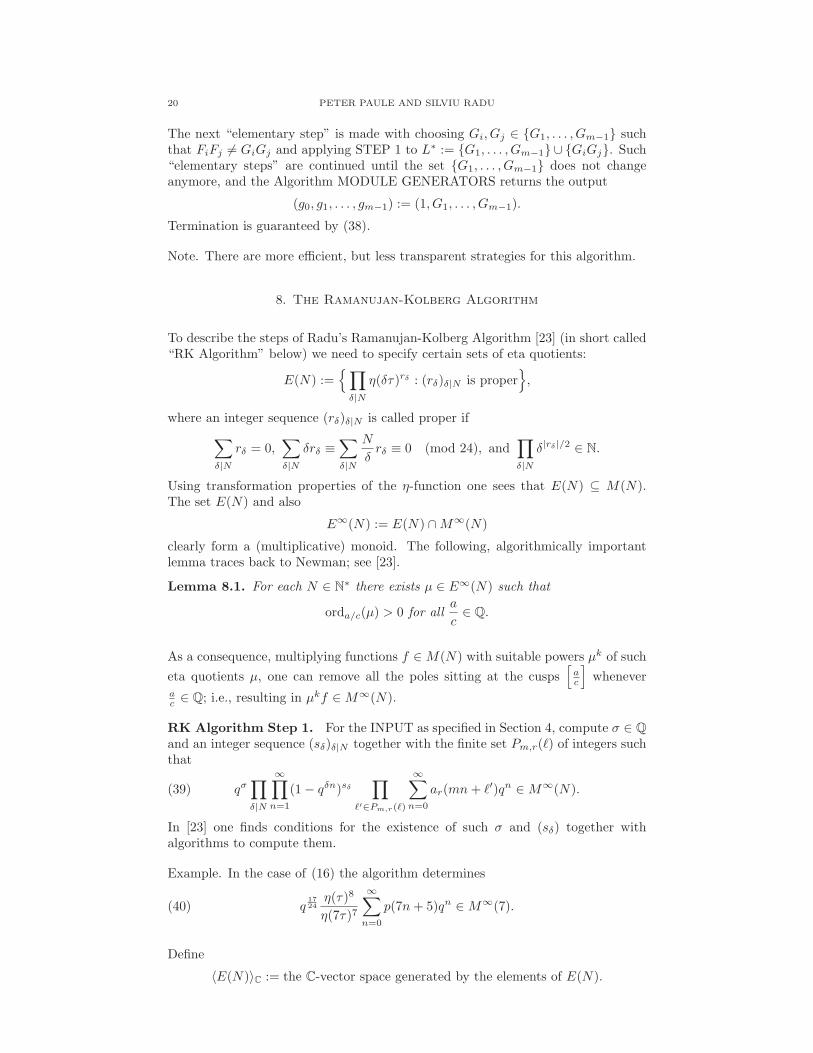
The next “elementary step” is made with choosing Gi, Gj ∈ G1, . . . , Gm−1 suchthat FiFj 6= GiGj and applying STEP 1 to L∗ := G1, . . . , Gm−1 ∪ GiGj. Such“elementary steps” are continued until the set G1, . . . , Gm−1 does not changeanymore, and the Algorithm MODULE GENERATORS returns the output
(g0, g1, . . . , gm−1) := (1, G1, . . . , Gm−1).
Termination is guaranteed by (38).
Note. There are more efficient, but less transparent strategies for this algorithm.
8. The Ramanujan-Kolberg Algorithm
To describe the steps of Radu’s Ramanujan-Kolberg Algorithm [23] (in short called“RK Algorithm” below) we need to specify certain sets of eta quotients:
E(N) :=
∏
δ|N
η(δτ)rδ : (rδ)δ|N is proper
,
where an integer sequence (rδ)δ|N is called proper if
∑
δ|N
rδ = 0,∑
δ|N
δrδ ≡∑
δ|N
N
δrδ ≡ 0 (mod 24), and
∏
δ|N
δ|rδ|/2 ∈ N.
Using transformation properties of the η-function one sees that E(N) ⊆ M(N).The set E(N) and also
E∞(N) := E(N) ∩M∞(N)
clearly form a (multiplicative) monoid. The following, algorithmically importantlemma traces back to Newman; see [23].
Lemma 8.1. For each N ∈ N∗ there exists µ ∈ E∞(N) such that
orda/c(µ) > 0 for alla
c∈ Q.
As a consequence, multiplying functions f ∈ M(N) with suitable powers µk of such
eta quotients µ, one can remove all the poles sitting at the cusps[
ac
]
wheneverac ∈ Q; i.e., resulting in µkf ∈ M∞(N).
RK Algorithm Step 1. For the INPUT as specified in Section 4, compute σ ∈ Q
and an integer sequence (sδ)δ|N together with the finite set Pm,r(ℓ) of integers suchthat
(39) qσ∏
δ|N
∞∏
n=1
(1− qδn)sδ∏
ℓ′∈Pm,r(ℓ)
∞∑
n=0
ar(mn+ ℓ′)qn ∈ M∞(N).
In [23] one finds conditions for the existence of such σ and (sδ) together withalgorithms to compute them.
Example. In the case of (16) the algorithm determines
(40) q1724
η(τ)8
η(7τ)7
∞∑
n=0
p(7n+ 5)qn ∈ M∞(7).
Define
〈E(N)〉C := the C-vector space generated by the elements of E(N).
PARTITION ANALYSIS, MODULAR FUNCTIONS, AND COMPUTER ALGEBRA 21
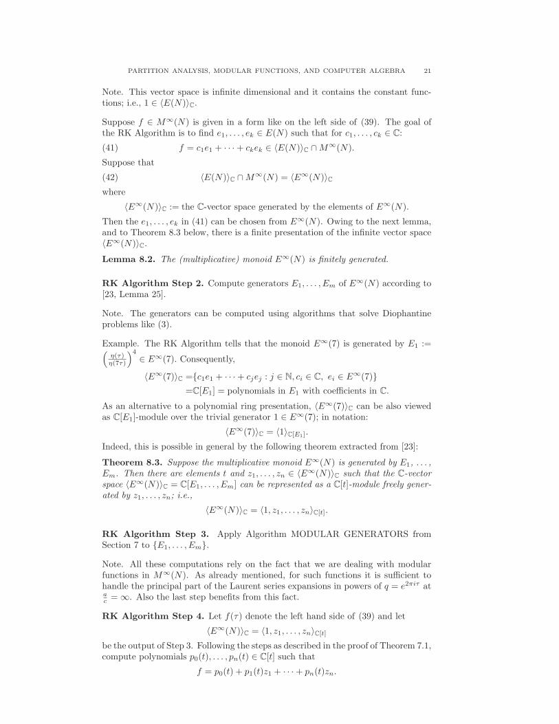
Note. This vector space is infinite dimensional and it contains the constant func-tions; i.e., 1 ∈ 〈E(N)〉C.
Suppose f ∈ M∞(N) is given in a form like on the left side of (39). The goal ofthe RK Algorithm is to find e1, . . . , ek ∈ E(N) such that for c1, . . . , ck ∈ C:
(41) f = c1e1 + · · ·+ ckek ∈ 〈E(N)〉C ∩M∞(N).
Suppose that
(42) 〈E(N)〉C ∩M∞(N) = 〈E∞(N)〉C
where
〈E∞(N)〉C := the C-vector space generated by the elements of E∞(N).
Then the e1, . . . , ek in (41) can be chosen from E∞(N). Owing to the next lemma,and to Theorem 8.3 below, there is a finite presentation of the infinite vector space〈E∞(N)〉C.
Lemma 8.2. The (multiplicative) monoid E∞(N) is finitely generated.
RK Algorithm Step 2. Compute generators E1, . . . , Em of E∞(N) according to[23, Lemma 25].
Note. The generators can be computed using algorithms that solve Diophantineproblems like (3).
Example. The RK Algorithm tells that the monoid E∞(7) is generated by E1 :=(
η(τ)η(7τ)
)4
∈ E∞(7). Consequently,
〈E∞(7)〉C =c1e1 + · · ·+ cjej : j ∈ N, ci ∈ C, ei ∈ E∞(7)
=C[E1] = polynomials in E1 with coefficients in C.
As an alternative to a polynomial ring presentation, 〈E∞(7)〉C can be also viewedas C[E1]-module over the trivial generator 1 ∈ E∞(7); in notation:
〈E∞(7)〉C = 〈1〉C[E1].
Indeed, this is possible in general by the following theorem extracted from [23]:
Theorem 8.3. Suppose the multiplicative monoid E∞(N) is generated by E1, . . . ,Em. Then there are elements t and z1, . . . , zn ∈ 〈E∞(N)〉C such that the C-vectorspace 〈E∞(N)〉C = C[E1, . . . , Em] can be represented as a C[t]-module freely gener-ated by z1, . . . , zn; i.e.,
〈E∞(N)〉C = 〈1, z1, . . . , zn〉C[t].
RK Algorithm Step 3. Apply Algorithm MODULAR GENERATORS fromSection 7 to E1, . . . , Em.
Note. All these computations rely on the fact that we are dealing with modularfunctions in M∞(N). As already mentioned, for such functions it is sufficient tohandle the principal part of the Laurent series expansions in powers of q = e2πiτ atac = ∞. Also the last step benefits from this fact.
RK Algorithm Step 4. Let f(τ) denote the left hand side of (39) and let
〈E∞(N)〉C = 〈1, z1, . . . , zn〉C[t]
be the output of Step 3. Following the steps as described in the proof of Theorem 7.1,compute polynomials p0(t), . . . , pn(t) ∈ C[t] such that
f = p0(t) + p1(t)z1 + · · ·+ pn(t)zn.

22 PETER PAULE AND SILVIU RADU
Example. Define∞∑
k=0
L(k)qk :=
∞∏
j=1
1
1− q2j−1=
∞∏
j=1
1− q2j
1− qj.
Note. This is the generating function of partitions into odd parts; we started withthe Lecture Hall partition problem (2) where such partitions arise but with a re-striction on the size of the parts.
RK Step 1 with M = 2, r = (r1, r2) = (−1, 1), m = 7, and ℓ = 3 delivers Pm,r(3) =3, 4, 6 and
q−5∞∏
j=1
(1− qj)13(1− q7j)8
(1− q2j)5(1− q14j)16
×∞∑
n=0
L(7n+ 3)qn ·∞∑
n=0
L(7n+ 4)qn ·∞∑
n=0
L(7n+ 6)qn ∈ M∞(14).
(43)
RK Step 2 gives that the multiplicative monoid E∞(14) is generated by
E1 =
(
η(2τ)
η(τ)
)1(η(7τ)
η(τ)
)7(η(14τ)
η(τ)
)−1
∈ E∞(14),
E2 =
(
η(2τ)
η(τ)
)8(η(7τ)
η(τ)
)4(η(14τ)
η(τ)
)−8
∈ E∞(14),
E3 =
(
η(2τ)
η(τ)
)−5(η(7τ)
η(τ)
)5(η(14τ)
η(τ)
)−13
∈ E∞(14),
E4 =
(
η(2τ)
η(τ)
)1(η(7τ)
η(τ)
)3(η(14τ)
η(τ)
)−7
∈ E∞(14),
E5 =
(
η(2τ)
η(τ)
)5(η(7τ)
η(τ)
)7(η(14τ)
η(τ)
)−11
∈ E∞(14),
and
E6 =
(
η(2τ)
η(τ)
)−2(η(7τ)
η(τ)
)6(η(14τ)
η(τ)
)−10
∈ E∞(14).
RK Step 3 computes that
〈E∞(14)〉C = 〈1, E4〉C[E1];
i.e., t = E1, z1 = E4. Denoting the function in (43) by f , RK Step 4 outputs
f = 8(p0(t) + p1(t)z1)
where p0(t) = −16t+ 9t2 and p1(t) = 2t.
Note. It is easily checked that this relation implies for all n ∈ N:
(44) L(7n+ 3) ≡ L(7n+ 4) ≡ L(7n+ 6) ≡ 0 (mod 2).
In a different setting, Gordon and Ono [11] have shown the strikingly general resultthat almost all values of L(n) are divisible by 2k for any k ∈ N.
Radu’s “Ramanujan-Kolberg” package also delivers that∞∑
n=0
L(7n)qn ·
∞∑
n=0
L(7n+ 1)qn ·
∞∑
n=0
L(7n+ 5)qn
=q6∞∏
j=1
(1− q2j)5(1− q14j)16
(1− qj)13(1− q7j)8(3E3
1 + 24E21 + 64E1)
PARTITION ANALYSIS, MODULAR FUNCTIONS, AND COMPUTER ALGEBRA 23
and∞∑
n=0
L(7n+ 2)qn = q3∞∏
n=1
(1− q14j)8
(1− qj)3(1− q2j)(1− q7j)4(8E1 + E4 − 8).
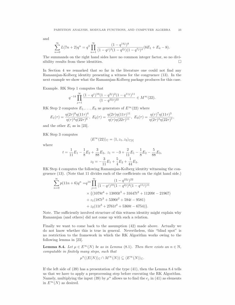
The summands on the right hand sides have no common integer factor, so no divi-sibility results from these identities.
In Section 4 we remarked that so far in the literature one could not find anyRamanujan-Kolberg identity presenting a witness for the congruence (13). In thenext example we show what the Ramanujan-Kolberg package produces for this case.
Example. RK Step 1 computes that
q−14∞∏
j=1
(1− qj)10(1− q2j)2(1− q11j)11
(1− q22j)22∈ M∞(22).
RK Step 2 computes E1, . . . , E8 as generators of E∞(22) where
E1(τ) =η(2τ)8η(11τ)4
η(τ)4η(22τ)8, E2(τ) =
η(2τ)η(11τ)11
η(τ)η(22τ)11, E3(τ) =
η(τ)7η(11τ)3
η(2τ)3η(22τ)7,
and the other Ei as in [23].
RK Step 3 computes
〈E∞(22)〉C = 〈1, z1, z2〉C[t]
where
t =1
11E1 −
1
8E2 +
3
88E3, z1 = −3 +
2
11E1 −
1
8E2 −
5
88E3,
z2 = −3
11E1 +
5
4E2 +
1
44E3.
RK Step 4 computes the following Ramanujan-Kolberg identity witnessing the con-gruence (13). (Note that 11 divides each of the coefficients on the right hand side.)
∞∑
n=0
p(11n+ 6)qn =q14∞∏
j=1
(1− q22j)22
(1− qj)10(1− q2j)2(1− q11j)11
× (1078t4 + 13893t3 + 31647t2 + 11209t− 21967)
+ z1(187t3 + 5390t2 + 594t− 9581)
+ z2(11t3 + 2761t2 + 5368t− 6754).
Note. The sufficiently involved structure of this witness identity might explain whyRamanujan (and others) did not come up with such a relation.
Finally we want to come back to the assumption (42) made above. Actually wedo not know whether this is true in general. Nevertheless, this “blind spot” isno restriction to the framework in which the RK Algorithm works owing to thefollowing lemma in [23].
Lemma 8.4. Let µ ∈ E∞(N) be as in Lemma (8.1). Then there exists an n ∈ N,computable in finitely many steps, such that
µn(〈E(N)〉C ∩M∞(N)) ⊆ 〈E∞(N)〉C.
If the left side of (39) has a presentation of the type (41), then the Lemma 8.4 tellsus that we have to apply a preprocessing step before executing the RK Algorithm.Namely, multiplying the input (39) by µn allows us to find the ej in (41) as elementsin E∞(N) as desired.

24 PETER PAULE AND SILVIU RADU
References
[1] George E. Andrews. The Selected Works of George E. Andrews, volume 3 of ICP Selected
Papers. Imperial College Press, London, 2013. With commentary, edited by Andrew V. Sills.[2] George E. Andrews and Peter Paule. MacMahon’s Partition Analyis XII: Plane partitions.
Journal of the London Mathematical Society, 76:647–666, 2007.[3] George E. Andrews and Peter Paule. MacMahon’s Partition Analysis XI: Broken diamonds
and modular forms. Acta Arithmetica, 126:281–294, 2007.[4] George E. Andrews and Peter Paule. MacMahon’s Dream, pages 1–12. Partitions, q-series,
and Modular Forms, volume 23 of Developments in Mathematics. Springer, 2012.[5] George E. Andrews, Peter Paule, and Axel Riese. MacMahon’s Partition Analysis III: The
Omega package. European Journal of Combinatorics, 22:887–904, 2001.[6] George E. Andrews, Peter Paule, and Axel Riese. MacMahon’s Partition Analysis VI: A New
reduction algorithm. Annals of Combinatorics, 5:251–270, 2001.
[7] Felix Breuer and Zafeirakis Zafeirakopoulos. Polyhedral Omega: A new algorithm for solvinglinear diophantine systems. arXiv:1501.07773, 2015.
[8] Song Heng Chan. Some congruences for Andrews-Paule’s broken 2-diamond partitions. Dis-crete Mathematics, 308:5735–5741, 2008.
[9] William Y. C. Chen, Anna R. B. Fan, and Rebecca T. Yu. Ramanujan-type congruences forbroken 2-diamond partitions modulo 3. Science China Mathematics, 57:1553–1560, 2014.
[10] Fred Diamond and Jerry Shurman. A First Course in Modular Forms. Springer, 2005.[11] Basil Gordon and Ken Ono. Divisibility properties of certain partition functions by powers of
primes. The Ramanujan Journal, 1:25–35, 1997.[12] H.J. Grace and A. Young. The Algebra of Invariants. Cambridge University Press, 1903.[13] G. H. Hardy, P. V. S. Aiyar, and B. M. Wilson. Collected Papers of Srinivasa Ramanujan.
AMS Chelsea Publishing Series. AMS Chelsea Publishing, 1927.[14] Michael D. Hirschhorn and James Sellers. On recent congruence results of Andrews and Paule
for broken k-diamonds. Bulletin of the Australian Mathematical Society, 75:121–126, 2007.[15] Marvin I. Knopp. Modular Functions in Analytic Number Theory, volume 337. AMS Chelsea
Publishing, 1993.[16] Oggmund Kolberg. Some identities involving the partition function. Mathematica Scandinav-
ica, 5:77–92, 1957.
[17] Gerard Ligozat. Courbes modulaires de genre 1. Memoires de la S.M.F, 43:5–80, 1975.[18] P.A. MacMahon. Combinatory Analysis, volume I, II. Chelsea, 3 edition, 1984.[19] Rick Miranda. Algebraic Curves and Riemann Surfaces, volume 5 of Graduate Studies in
Mathematics. AMS, 1995.
[20] Ken Ono. The Web of Modularity: Arithmetic of the Coefficients of Modular Forms and q-Series, volume 102 of CBMS Regional Conference Series in Mathematics. Washington, DC,2004.
[21] George Polya.Mathematics and Plausible Reasoning: Induction and Analogy in Mathematics,volume 1. Princeton University Press, Princeton, New Jersey, 1954.
[22] Hans Rademacher. The Ramanujan identities under modular substitutions. Transactions ofthe American Mathematical Society, 51:609–636, 1942.
[23] Cristian-Silviu Radu. An algorithmic approach to Ramanujan-Kolberg identities. Journal ofSymbolic Computation, 68:1–33, 2014.
[24] S. Ramanujan. Some properties of p(n), the number of partitions of n. Proceedings CambridgePhilosophical Society, 19:207–210, 1919.
[25] J.C. Rosales, P. Garcıa-Sanchez, J.I. Garcıa-Garcıa, and M.B. Branko. Systems of inequalitiesand numerical semigroups. Journal of London Mathematical Society, 65:611–623, 2002.
[26] Gouce Xin. An Euclid style algorithm for MacMahon’s partition analysis. Journal of Combi-
natorial Theory A, 318:32–60, 2015.[27] Doron Zeilberger. George Eyre Andrews (b. Dec. 4, 1938): A Reluctant REVOLUTIONARY
(Part 1). vimeo.com/81396551. Rutgers Experimental Mathematics Seminar, December 5,2013.
[28] Doron Zeilberger. George Eyre Andrews (b. Dec. 4, 1938): A Reluctant REVOLUTIONARY(Part 2). vimeo.com/81410565. Rutgers Experimental Mathematics Seminar, December 5,2013.
Research Institute for Symbolic Computation (RISC), Johannes Kepler University, A-4040 Linz, Austria
Research Institute for Symbolic Computation (RISC), Johannes Kepler University, A-4040 Linz, Austria