identification of significant factors affecting stormwater...

Stormwater and Urban Water Systems Modeling Proceedings, Monograph 14. (edited by W. James, K.N. Irvine, E.A. McBean, and R.E. Pitt). CHI. Guelph, Ontario, pp. 287 –

326, 2006. 1

1

1

Identification of Significant Factors Affecting Stormwater Quality Using the NSQD

Alexander Maestre, Robert Pitt

1 Introduction The normal approach to classify urban sites for estimating stormwater characteristics is based on

land use. This approach is generally accepted because it is related to the activity in the watershed, plus many site features are generally consistent within each land use. Two drainage areas with the same size, percentage of imperviousness, ground slope, sampling methods, and stormwater controls will produce different stormwater concentrations if the main activity in one watershed is an automobile manufacturing facility (industrial land use) while the other is a shopping center (commercial land use) for example. There will likely be higher concentrations of metals at the industrial site due to the manufacturing processes, while the commercial site may have higher concentrations of PAHs (polycyclic aromatic hydrocarbons) due to the frequency and numbers of customer automobiles entering and leaving the parking lots.

Previous studies indicated that there are significant differences in stormwater constituents for different land use categories (Pitt et al. 2004). This is supported for other databases like NURP (EPA 1983), CDM (Smullen and Cave, 2002) and USGS (Driver et al., 1985). The main question to be addressed in this chapter is if there is a different classification method that better describes stormwater quality, possibly by also considering such factors as geographical area (EPA Rain Zone), season, percentage of imperviousness, watershed area, type of conveyance, controls in the watershed, sampling method, and type of sample compositing, and possible interactions between these factors.

This chapter presents several approaches to explain the variability of stormwater quality by considering these additional factors. Maestre (2005b) has shown that ignoring the non-detected observations can adversely affect the mean, median and standard deviations of the dataset, and the resulting statistical test results. Therefore, the calculations presented in this chapter used the censored observations using the Cohen’s maximum likelihood method.

2 Main Factors Affecting Stormwater Quality The EPA Rain Zone (geographical location), percentage of imperviousness, land use, type of conveyance, controls in the watershed, sample analysis method, and type of sampling procedures were selected as potential influencing factors affecting stormwater quality for the preliminary analyses. Data from sites having single land uses will be used in the basic analyses. Data from the mixed land use sites could be used for verification. The first step was to inventory the total number of events in each of the possible combinations of these factors. The EPA Rain Zone, land use, type of conveyance, type of controls present in the watershed, sampling methods and type of compositing procedures are

2

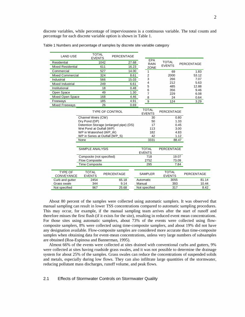
discrete variables, while percentage of imperviousness is a continuous variable. The total counts and percentage for each discrete variable option is shown in Table 1.

Table 1 Numbers and percentage of samples by discrete site variable category

LAND USE TOTAL EVENTS PERCENTAGE

Residential 1042 27.68 Mixed Residential 611 16.23 Commercial 527 14.00 Mixed Commercial 324 8.61 Industrial 566 15.03 Mixed Industrial 249 6.61 Institutional 18 0.48 Open Space 49 1.30 Mixed Open Space 168 4.46 Freeways 185 4.91 Mixed Freeways 26 0.69

TYPE OF CONTROL TOTAL EVENTS

PERCENTAGE

Channel Weirs (CW) 30 0.80 Dry Pond (DP) 50 1.33 Detention Storage (enlarged pipe) (DS) 17 0.45 Wet Pond at Outfall (WP) 113 3.00 WP in Watershed (WP_W) 182 4.83 WP in Series at Outfall (WP_S) 42 1.12 None 3331 88.47

SAMPLE ANALYSIS TOTAL

EVENTS PERCENTAGE

Composite (not specified) 718 19.07 Flow Composite 2752 73.09 Time Composite 295 7.84

About 80 percent of the samples were collected using automatic samplers. It was observed that

manual sampling can result in lower TSS concentrations compared to automatic sampling procedures. This may occur, for example, if the manual sampling team arrives after the start of runoff and therefore misses the first flush (if it exists for the site), resulting in reduced event mean concentrations. For those sites using automatic samplers, about 73% of the events were collected using flow-composite samplers, 8% were collected using time-composite samplers, and about 19% did not have any designation available. Flow-composite samples are considered more accurate than time-composite samples when obtaining data for event-mean concentrations, unless very large numbers of subsamples are obtained (Roa-Espinosa and Bannerman, 1995).

Almost 66% of the events were collected at sites drained with conventional curbs and gutters, 9% were collected at sites having roadside grass swales, and it was not possible to determine the drainage system for about 25% of the samples. Grass swales can reduce the concentrations of suspended solids and metals, especially during low flows. They can also infiltrate large quantities of the stormwater, reducing pollutant mass discharges, runoff volume, and peak flows.

2.1 Effects of Stormwater Controls on Stormwater Quality

EPA RAIN ZONE

TOTAL EVENTS PERCENTAGE

1 69 1.83 2 2000 53.12 3 266 7.07 4 212 5.63 5 485 12.88 6 356 9.46 7 229 6.08 8 24 0.64 9 124 3.29

TYPE OF CONVEYANCE

TOTAL EVENTS PERCENTAGE

Curb and gutter 2454 65.18 Grass swale 344 9.14 Not specified 967 25.68

SAMPLER TOTAL EVENTS

PERCENTAGE

Automatic 3055 81.14 Manual 393 10.44 Not specified 317 8.42

3

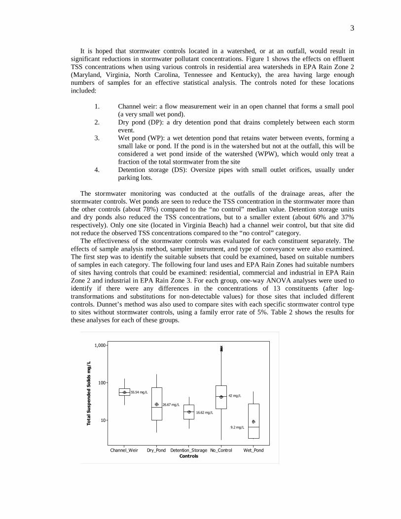
It is hoped that stormwater controls located in a watershed, or at an outfall, would result in significant reductions in stormwater pollutant concentrations. Figure 1 shows the effects on effluent TSS concentrations when using various controls in residential area watersheds in EPA Rain Zone 2 (Maryland, Virginia, North Carolina, Tennessee and Kentucky), the area having large enough numbers of samples for an effective statistical analysis. The controls noted for these locations included:

1. Channel weir: a flow measurement weir in an open channel that forms a small pool

(a very small wet pond). 2. Dry pond (DP): a dry detention pond that drains completely between each storm

event. 3. Wet pond (WP): a wet detention pond that retains water between events, forming a

small lake or pond. If the pond is in the watershed but not at the outfall, this will be considered a wet pond inside of the watershed (WPW), which would only treat a fraction of the total stormwater from the site

4. Detention storage (DS): Oversize pipes with small outlet orifices, usually under parking lots.

The stormwater monitoring was conducted at the outfalls of the drainage areas, after the

stormwater controls. Wet ponds are seen to reduce the TSS concentration in the stormwater more than the other controls (about 78%) compared to the “no control” median value. Detention storage units and dry ponds also reduced the TSS concentrations, but to a smaller extent (about 60% and 37% respectively). Only one site (located in Virginia Beach) had a channel weir control, but that site did not reduce the observed TSS concentrations compared to the “no control” category.

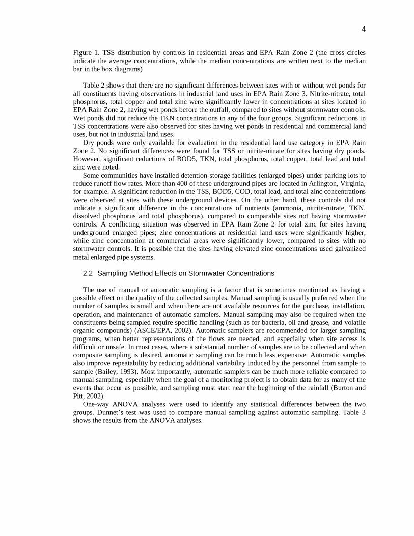
The effectiveness of the stormwater controls was evaluated for each constituent separately. The effects of sample analysis method, sampler instrument, and type of conveyance were also examined. The first step was to identify the suitable subsets that could be examined, based on suitable numbers of samples in each category. The following four land uses and EPA Rain Zones had suitable numbers of sites having controls that could be examined: residential, commercial and industrial in EPA Rain Zone 2 and industrial in EPA Rain Zone 3. For each group, one-way ANOVA analyses were used to identify if there were any differences in the concentrations of 13 constituents (after log-transformations and substitutions for non-detectable values) for those sites that included different controls. Dunnet’s method was also used to compare sites with each specific stormwater control type to sites without stormwater controls, using a family error rate of 5%. Table 2 shows the results for these analyses for each of these groups.

Controls

Tota

l Suspended S

olid

s m

g/L

Wet_PondNo_ControlDetention_StorageDry_PondChannel_Weir

1,000

100

10

9.2 mg/L

42 mg/L

16.62 mg/L

26.67 mg/L

55.54 mg/L

4

Figure 1. TSS distribution by controls in residential areas and EPA Rain Zone 2 (the cross circles indicate the average concentrations, while the median concentrations are written next to the median bar in the box diagrams)

Table 2 shows that there are no significant differences between sites with or without wet ponds for

all constituents having observations in industrial land uses in EPA Rain Zone 3. Nitrite-nitrate, total phosphorus, total copper and total zinc were significantly lower in concentrations at sites located in EPA Rain Zone 2, having wet ponds before the outfall, compared to sites without stormwater controls. Wet ponds did not reduce the TKN concentrations in any of the four groups. Significant reductions in TSS concentrations were also observed for sites having wet ponds in residential and commercial land uses, but not in industrial land uses.

Dry ponds were only available for evaluation in the residential land use category in EPA Rain Zone 2. No significant differences were found for TSS or nitrite-nitrate for sites having dry ponds. However, significant reductions of BOD5, TKN, total phosphorus, total copper, total lead and total zinc were noted.

Some communities have installed detention-storage facilities (enlarged pipes) under parking lots to reduce runoff flow rates. More than 400 of these underground pipes are located in Arlington, Virginia, for example. A significant reduction in the TSS, BOD5, COD, total lead, and total zinc concentrations were observed at sites with these underground devices. On the other hand, these controls did not indicate a significant difference in the concentrations of nutrients (ammonia, nitrite-nitrate, TKN, dissolved phosphorus and total phosphorus), compared to comparable sites not having stormwater controls. A conflicting situation was observed in EPA Rain Zone 2 for total zinc for sites having underground enlarged pipes; zinc concentrations at residential land uses were significantly higher, while zinc concentration at commercial areas were significantly lower, compared to sites with no stormwater controls. It is possible that the sites having elevated zinc concentrations used galvanized metal enlarged pipe systems.

2.2 Sampling Method Effects on Stormwater Concentrations The use of manual or automatic sampling is a factor that is sometimes mentioned as having a

possible effect on the quality of the collected samples. Manual sampling is usually preferred when the number of samples is small and when there are not available resources for the purchase, installation, operation, and maintenance of automatic samplers. Manual sampling may also be required when the constituents being sampled require specific handling (such as for bacteria, oil and grease, and volatile organic compounds) (ASCE/EPA, 2002). Automatic samplers are recommended for larger sampling programs, when better representations of the flows are needed, and especially when site access is difficult or unsafe. In most cases, where a substantial number of samples are to be collected and when composite sampling is desired, automatic sampling can be much less expensive. Automatic samples also improve repeatability by reducing additional variability induced by the personnel from sample to sample (Bailey, 1993). Most importantly, automatic samplers can be much more reliable compared to manual sampling, especially when the goal of a monitoring project is to obtain data for as many of the events that occur as possible, and sampling must start near the beginning of the rainfall (Burton and Pitt, 2002).

One-way ANOVA analyses were used to identify any statistical differences between the two groups. Dunnet’s test was used to compare manual sampling against automatic sampling. Table 3 shows the results from the ANOVA analyses.

Tab

le 2

One

-Way

AN

OV

A R

esul

ts b

y C

ontr

ol T

ype

Res

iden

tial L

and

Use

, EP

A R

ain

Zon

e 2

Com

mer

cial

Lan

d U

se, E

PA

Rai

n Z

one

2 In

dust

rial E

PA

Rai

n Z

one

2 R

esid

entia

l EP

A R

ain

Zon

e 3

Con

stitu

ent

No

Con

trol

W

eir

DP

D

S

WP

p-

valu

ea N

o C

ontr

ol

DS

W

P

WP

W

p-va

lue

No

Con

trol

W

P

p-va

lue

No

Con

trol

W

P

p-va

lue

Har

dn

ess

mg

/L

30.7

7 (6

1) b

- -

44.3

8 (7

,=)

66.4

5 (1

0,>)

0.

024

58.9

7 (3

5)

58.1

7 (8

,=)

71.8

0 (1

1,=)

47

.11

(9,=

) 0.

717

- -

Non

e -

- N

one

Oil

and

G

reas

e m

g/L

2.38

(2

02)

2.50

(3

,=)

2.68

(3

,=)

2.19

(9

,=)

2.50

(1

3,=)

0.

999

4.20

(1

00)

1.84

(8

,=)

2.84

(1

7,=)

3.

36

(13,

=)

0.08

2 3.

85

(81)

1.

43

(37,

<)

0 -

- N

one

TD

S m

g/L

62

.42

(424

) 11

2.80

(2

9.>)

58

.88

(3,=

) 98

.45

(8,=

) 12

0.39

(1

2,>)

0

74.8

9 (1

74)

100.

69

(8,=

) 89

.99

(26,

=)

71.1

2 (1

3,=)

0.

477

- -

Non

e 69

.53

(44)

49

.84

(25,

=)

0.11

2

TS

S m

g/L

40

.10

(559

) 55

.54

(29,

=)

26.6

7 (2

1,=)

14

.46

(9,<

) 9.

25

(12,

<)

0 48

.13

(244

) 19

.54

(8,<

) 19

.47

(26,

<)

16.8

5 (1

3,<)

0

51.9

6 (2

05)

48.0

5 (2

9,=)

0.

693

48.3

5 (4

4)

70.4

0 (2

5,=)

0.

281

BO

D m

g/L

11

.07

(533

) 6.

16

(29,

<)

3.44

(2

1,<)

3.

66

(9,<

) 3.

10

(21,

<)

0 14

.66

(241

) 4.

44

(8,<

) 7.

06

(26,

<)

5.41

(1

2,<)

0

10.6

3 (2

00)

9.30

(2

9)

0.46

6 6.

41

(44)

5.

14

(23,

=)

0.22

1

CO

D m

g/L

56

.91

(418

) 49

.02

(29,

=)

33.4

5 (3

,=)

22.1

7 (9

,<)

24.5

8 (1

2,<)

0

73.6

2 (1

74)

27.1

8 (8

,<)

35.9

9 (2

6,<)

23

.88

(13,

<)

0 -

- N

one

37

(44)

43

.06

(25,

=)

0.39

5

Am

mo

nia

m

g/L

0.

24

(409

) 0.

05

(29,

<)

0.41

(3

,=)

0.40

(9

,=)

0.07

(1

2,<)

0

0.39

(1

74)

0.30

(8

,=)

0.13

(2

6,<)

0.

16

(13,

<)

0 -

- N

one

0.12

(3

) 0.

03

(25,

=)

0.16

5

NO

2 +

NO

3 m

g/L

0.

54

(546

) 0.

05

(29,

<)

0.59

(2

1,=)

0.

98

(9,=

) 0.

28

(12,

<)

0 0.

60

(242

) 1.

18

(8,=

) 0.

48

(26,

=)

0.22

(1

3,<)

0

0.61

(1

97)

0.30

(2

9,<)

0

0.57

(3

0)

0.40

(2

5,=)

0.

193

TK

N m

g/L

1.

34

(549

) 1.

49

(29,

=)

0.79

(2

1,<)

1.

38

(9,=

) 1.

04

(12,

=)

0.01

2 1.

59

(241

) 1.

04

(8,=

) 1.

19

(26,

=)

1.03

(1

3,=)

0.

057

1.22

(1

98)

0.98

(2

9,=)

0.

166

1.18

(4

3)

1.12

(2

5,=)

0.

807

Dis

solv

ed

Ph

osp

ho

rus

mg

/L

0.14

(4

04)

0.04

(2

9,<)

0.

15

(3,=

) 0.

11

(8,=

) 0.

03

(12.

<)

0 0.

11

(161

) 0.

09

(7,=

) 0.

05

(25,

=)

0.03

(1

3,=)

0

- -

Non

e 0.

07

(39)

0.

06

(25,

=)

0.19

1

To

tal

Ph

osp

ho

rus

mg

/L

0.30

(5

50)

0.23

(2

9,=)

0.

12

(21,

<)

0.15

(9

,<)

0.07

(1

2, <

) 0

0.25

(2

38)

0.16

(8

,=)

0.13

(2

6,<)

0.

08

(13,

<)

0 0.

23

(200

) 0.

09

(29,

<)

0 0.

16

(43)

0.

19

(25,

=)

0.43

8

To

tal

Co

pp

er

µg

/L

11.0

1 (4

03)

2.69

(3

,<)

6.16

(2

1,<)

20

,75

(9,>

) 3.

13

(4,<

) 0

17.5

3 (1

94)

14.1

4 (8

,=)

5.57

(6

,<)

6.00

(4

,<)

0 16

.00

(150

) 7.

38

(29,

<)

0 16

.66

(38)

12

.58

(25,

=)

0.10

6

To

tal L

ead

µ

g/L

7.

73

(364

) 6.

41

(3,<

) 1.

50

(21,

<)

1.16

(9

,<)

1.00

(4

,<)

0 16

.41

(194

) 1.

61

(8,<

) 4.

90

(7,<

) 2.

49

(4,<

) 0

11.1

6 (1

42)

8.66

(2

9,=)

0.

353

8.49

(3

1)

6.73

(2

5,=)

0.

454

To

tal Z

inc

µg

/L

67.5

6 (4

05)

4.11

(3

,<)

29.6

3 (2

1,<)

10

3.25

(9

,>)

10.4

4 (4

,<)

0 18

8.02

(1

97)

82.5

7 (8

,<)

44.2

6 (7

,<)

39.6

8 (4

,<)

0 18

0.01

(1

57)

60.4

4 (2

9,<)

0

143.

28

(38)

15

6.93

(2

5,=)

0.

608

Not

e.

a. T

he

bold

, ita

liciz

ed p

roba

bilit

y va

lues

indi

cat

e “s

tatis

tical

ly s

igni

fica

nt”

findi

ngs

at th

e 0.

05 le

vel

, or

bet

ter.

b. S

am

ple

size

an

d re

sult

from

Dun

net

te

st

com

parin

g if

site

s w

ith c

ontr

ol p

rodu

ces

larg

er c

once

ntr

atio

ns “

>”,

sm

alle

r co

nce

ntr

atio

ns

“<”

or n

ot s

tatis

tic

ally

diff

eren

ce “

=”

than

site

s w

ithou

t co

ntro

l a

t a fa

mily

err

or o

f 5%

.“N

one”

indi

cate

s n

o sa

mpl

es w

ere

colle

cted

for

this

con

stitu

ent i

n th

e gr

oup.

5

6

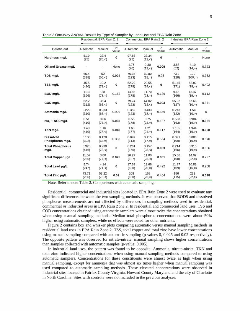
Table 3 One-Way ANOVA Results by Type of Sampler by Land Use and EPA Rain Zone

Residential, EPA Rain Z. 2 Commercial, EPA Rain Z. 2 Industrial EPA Rain Zone 2

Constituent Automatic Manual p-value Automatic Manual p-

value Automatic Manual p-value

Hardness mg/L 51.9 (23)

22.4 (28,<) 0

97.86 (23)

22.34 (12,<) 0 - - None

Oil and Grease mg/L - - None 4.75 (70)

2.30 (19,<) 0.009

3.68 (62)

4.10 (14,=) 0.723

TDS mg/L 65.4 (318)

50 (66,<) 0.004

76.36 (123)

60.80 (18,=) 0.25

73.2 (128)

100 (100,=) 0.362

TSS mg/L 45.5 (420)

19.2 (78,<) 0

52.29 (179)

20.55 (24,<) 0

51.45 (171)

62.82 (19,=) 0.402

BOD mg/L 11.3 (396)

9.8 (78,=) 0.162

14.86 (178)

11.70 (23,=) 0.189

9.65 (166)

13.47 (19,=) 0.112

COD mg/L 62.2 (312)

36.4 (66,<) 0

79.74 (123)

44.02 (18,<) 0.003

55.02 (127)

67.68 (10,=) 0.371

Ammonia mg/L 0.229 (310)

0.233 (66,=) 0.909

0.359 (123)

0.433 (18,=) 0.569

0.243 (122)

1.54 (10,>) 0

NO2 + NO3 mg/L 0.51 (410)

0.66 (75,>) 0.005

0.55 (178)

0.75 (23,=) 0.137

0.558 (163)

0.904 (19,>) 0.021

TKN mg/L 1.40 (410)

1.16 (78,<) 0.048

1.63 (177)

1.21 (24,=) 0.117

1.135 (164)

1.944 (19,>) 0.008

Dissolved Phosphorus mg/L

0.136 (302)

0.120 (63,=) 0.308

0.097 (113)

0.115 (17,=) 0.554

0.091 (109)

0.086 (10,=) 0.870

Total Phosphorus mg/L

0.325 (416)

0.230 (73,<) 0

0.261 (176)

0.157 (23,<) 0.003

0.214 (166)

0.315 (19,=) 0.056

Total Copper µg/L 11.57 (256)

8.80 (77,<) 0.025

20.27 (127)

11.80 (23,<) 0.001

15.66 (108)

14.97 (22,=) 0.797

Total Lead µg/L 9.74 (247)

4.14 (71,<) 0

17.62 (130)

13.66 (20,=) 0.422

11.27 (109)

10.83 (16,=) 0.908

Total Zinc µg/L 73.71 (256)

53.22 (76,<) 0.02

208 (130)

168 (23,=) 0.404

156 (115)

233 (22,>) 0.028

Note. Refer to note Table 2. Comparisons with automatic sampling. Residential, commercial and industrial sites located in EPA Rain Zone 2 were used to evaluate any

significant differences between the two sampling methods. It was observed that BOD5 and dissolved phosphorus measurements are not affected by differences in sampling methods used in residential, commercial or industrial areas in EPA Rain Zone 2. In residential and commercial land uses, TSS and COD concentrations obtained using automatic samplers were almost twice the concentrations obtained when using manual sampling methods. Median total phosphorus concentrations were about 50% higher using automatic samplers, while no effects were noted for other nutrients.

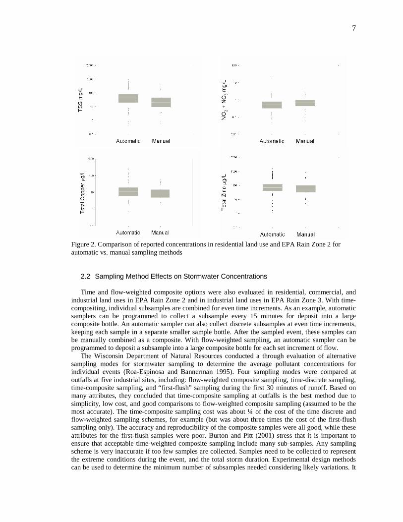
Figure 2 contains box and whisker plots comparing automatic versus manual sampling methods in residential land uses in EPA Rain Zone 2. TSS, total copper and total zinc have lower concentrations using manual sampling compared with automatic sampling (p-values 0, 0.025 and 0.02 respectively). The opposite pattern was observed for nitrate-nitrate, manual sampling shows higher concentrations than samples collected with automatic samples (p-value: 0.005).

In industrial land uses, the pattern was found to be opposite. Ammonia, nitrate-nitrite, TKN and total zinc indicated higher concentrations when using manual sampling methods compared to using automatic samplers. Concentrations for these constituents were almost twice as high when using manual sampling, except for ammonia that was almost six times higher when manual sampling was used compared to automatic sampling methods. These elevated concentrations were observed in industrial sites located in Fairfax County Virginia, Howard County Maryland and the city of Charlotte in North Carolina. Sites with controls were not included in the previous analyses.

7

Figure 2. Comparison of reported concentrations in residential land use and EPA Rain Zone 2 for automatic vs. manual sampling methods

2.2 Sampling Method Effects on Stormwater Concentrations Time and flow-weighted composite options were also evaluated in residential, commercial, and

industrial land uses in EPA Rain Zone 2 and in industrial land uses in EPA Rain Zone 3. With time-compositing, individual subsamples are combined for even time increments. As an example, automatic samplers can be programmed to collect a subsample every 15 minutes for deposit into a large composite bottle. An automatic sampler can also collect discrete subsamples at even time increments, keeping each sample in a separate smaller sample bottle. After the sampled event, these samples can be manually combined as a composite. With flow-weighted sampling, an automatic sampler can be programmed to deposit a subsample into a large composite bottle for each set increment of flow.

The Wisconsin Department of Natural Resources conducted a through evaluation of alternative sampling modes for stormwater sampling to determine the average pollutant concentrations for individual events (Roa-Espinosa and Bannerman 1995). Four sampling modes were compared at outfalls at five industrial sites, including: flow-weighted composite sampling, time-discrete sampling, time-composite sampling, and “first-flush” sampling during the first 30 minutes of runoff. Based on many attributes, they concluded that time-composite sampling at outfalls is the best method due to simplicity, low cost, and good comparisons to flow-weighted composite sampling (assumed to be the most accurate). The time-composite sampling cost was about ¼ of the cost of the time discrete and flow-weighted sampling schemes, for example (but was about three times the cost of the first-flush sampling only). The accuracy and reproducibility of the composite samples were all good, while these attributes for the first-flush samples were poor. Burton and Pitt (2001) stress that it is important to ensure that acceptable time-weighted composite sampling include many sub-samples. Any sampling scheme is very inaccurate if too few samples are collected. Samples need to be collected to represent the extreme conditions during the event, and the total storm duration. Experimental design methods can be used to determine the minimum number of subsamples needed considering likely variations. It

8

is more common to now include the use of “continuous” water quality probes at sampling locations, with in-situ observations obtained every few minutes. Unfortunately, these details were not available for the NSQD sampling sites; some sites may have had too few subsamples to represent the storm conditions, while others may have had sufficient numbers of subsamples. Also, most of the NSQD samples only represented the first 3 hours of runoff events. If events were longer, the later storm periods were likely not represented. These issues are discussed more in the next subsection.

One-way ANOVA tests were used to evaluate the presence of significant differences between these two composite sampling schemes. Dunnet’s comparison test was used to evaluate if concentrations associated with time-compositing were larger or lower than concentrations associated with flow- compositing. Table 4 shows the results of these tests.

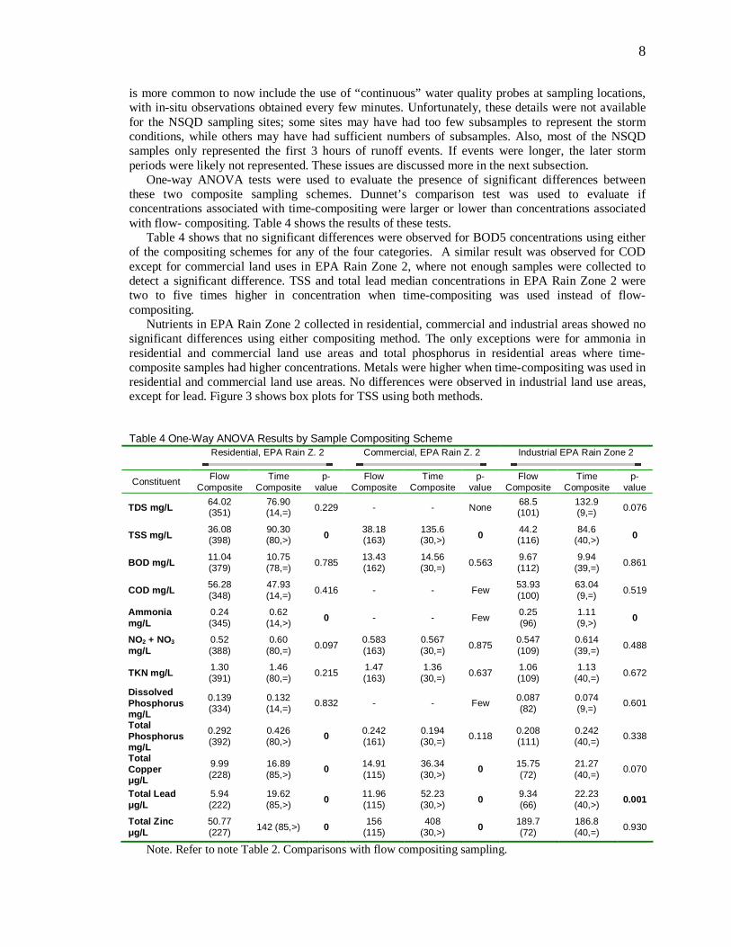
Table 4 shows that no significant differences were observed for BOD5 concentrations using either of the compositing schemes for any of the four categories. A similar result was observed for COD except for commercial land uses in EPA Rain Zone 2, where not enough samples were collected to detect a significant difference. TSS and total lead median concentrations in EPA Rain Zone 2 were two to five times higher in concentration when time-compositing was used instead of flow-compositing.

Nutrients in EPA Rain Zone 2 collected in residential, commercial and industrial areas showed no significant differences using either compositing method. The only exceptions were for ammonia in residential and commercial land use areas and total phosphorus in residential areas where time-composite samples had higher concentrations. Metals were higher when time-compositing was used in residential and commercial land use areas. No differences were observed in industrial land use areas, except for lead. Figure 3 shows box plots for TSS using both methods.

Table 4 One-Way ANOVA Results by Sample Compositing Scheme Residential, EPA Rain Z. 2 Commercial, EPA Rain Z. 2 Industrial EPA Rain Zone 2

Constituent Flow Composite

Time Composite

p-value

Flow Composite

Time Composite

p-value

Flow Composite

Time Composite

p-value

TDS mg/L 64.02 (351)

76.90 (14,=) 0.229 - - None

68.5 (101)

132.9 (9,=) 0.076

TSS mg/L 36.08 (398)

90.30 (80,>) 0

38.18 (163)

135.6 (30,>) 0

44.2 (116)

84.6 (40,>) 0

BOD mg/L 11.04 (379)

10.75 (78,=) 0.785

13.43 (162)

14.56 (30,=) 0.563

9.67 (112)

9.94 (39,=) 0.861

COD mg/L 56.28 (348)

47.93 (14,=) 0.416 - - Few

53.93 (100)

63.04 (9,=) 0.519

Ammonia mg/L

0.24 (345)

0.62 (14,>) 0 - - Few

0.25 (96)

1.11 (9,>) 0

NO2 + NO3 mg/L

0.52 (388)

0.60 (80,=) 0.097

0.583 (163)

0.567 (30,=) 0.875

0.547 (109)

0.614 (39,=) 0.488

TKN mg/L 1.30 (391)

1.46 (80,=) 0.215

1.47 (163)

1.36 (30,=) 0.637

1.06 (109)

1.13 (40,=) 0.672

Dissolved Phosphorus mg/L

0.139 (334)

0.132 (14,=)

0.832 - - Few 0.087 (82)

0.074 (9,=)

0.601

Total Phosphorus mg/L

0.292 (392)

0.426 (80,>)

0 0.242 (161)

0.194 (30,=)

0.118 0.208 (111)

0.242 (40,=)

0.338

Total Copper µg/L

9.99 (228)

16.89 (85,>)

0 14.91 (115)

36.34 (30,>)

0 15.75 (72)

21.27 (40,=)

0.070

Total Lead µg/L

5.94 (222)

19.62 (85,>) 0

11.96 (115)

52.23 (30,>) 0

9.34 (66)

22.23 (40,>) 0.001

Total Zinc µg/L

50.77 (227) 142 (85,>) 0

156 (115)

408 (30,>) 0

189.7 (72)

186.8 (40,=) 0.930

Note. Refer to note Table 2. Comparisons with flow compositing sampling.

9

Figure 3. Comparisons between time- and flow-composite options for TSS 2.4 Sampling Period During Runoff Event and Selection of Events to Sample Another potential factor that may affect stormwater quality is the sampling period during the

runoff event. Automatic samplers can initiate sampling very close to the beginning of flow, while manual sampling usually requires travel time and other delays before sampling can be started. It is also possible for automatic samplers to represent the complete storm, if of very long duration, as long as proper sampler setup programming is performed (Burton and Pitt 2001). However, automatic samplers are not capable of sampling bed load material, and are less effective in sampling larger particles (>500 µm) than typically suspended solids. Manual sampling, if able to collect a sample from a cascading flow, can collect from the complete particle size distribution.

The NPDES stormwater sampling protocols only required collecting composite samples over the first three hours of the event instead of during the whole event. Truncating the sampling before the runoff event ended may have adversely affected the measured stormwater quality.

Selecting a small subset of the annual events can also bias the monitoring results. In most stormwater research projects, the goal is to sample and analyze as many events as possible during the monitoring period. As a minimum, about 30 samples are usually desired in order to adequately determine the stormwater characteristics with an error level of about 25% (assuming 95% confidence and 80% power) (Burton and Pitt 2001). With only three events per year required per land use for the NPDES stormwater permits, the accuracy of the calculated EMC is questionable until many years have passed. Also, the three storms need to be randomly selected from the complete set of rains in order to be most statistically representative.

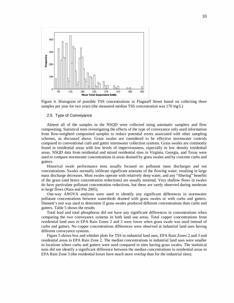
Flagstaff Street, in Prince George MD, had the most events collected for any site in the NSQD. They collected 28 events during two years of sampling (1998 and 1999). A statistical test was made choosing 6 events (three for each year) from this set, creating 5,600 different possibilities. Figure 4 shows the histogram of these possibilities. The median TSS of the 28 events was 170 mg/L, with a 95% confidence interval between 119 and 232 mg/L. Only 60% of the 5,600 possibilities were inside this confidence interval. Almost half (40%) of the possibilities for the observed EMC would therefore be outside the 95% confidence interval for the true median concentration if only three events were available for two years. As the number of samples increase, there will be a reduction in the bias of the EMC estimates. In Southern California, Leecaster (2002) determined that ten years of collecting three samples per year was required in order to reduce the error to 10% (Leecaster, 2002).

10

Mean Total Suspended Solids

Fre

quency

40536031527022518013590

400

300

200

100

0

Figure 4. Histogram of possible TSS concentrations in Flagstaff Street based on collecting three samples per year for two years (the measured median TSS concentration was 170 mg/L)

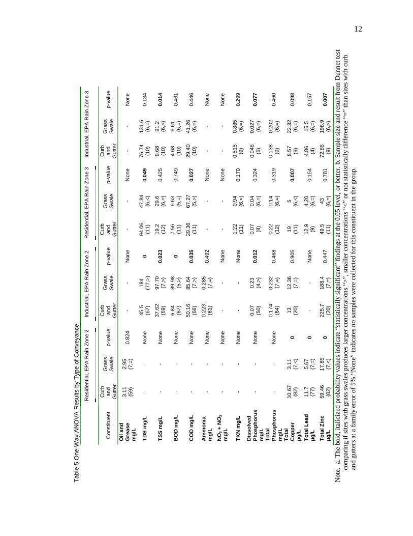
2.5 Type of Conveyance Almost all of the samples in the NSQD were collected using automatic samplers and flow

compositing. Statistical tests investigating the effects of the type of conveyance only used information from flow-weighted composited samples to reduce potential errors associated with other sampling schemes, as discussed above. Grass swales are considered to be effective stormwater controls compared to conventional curb and gutter stormwater collection systems. Grass swales are commonly found in residential areas with low levels of imperviousness, especially in low density residential areas. NSQD data from residential and mixed residential sites in Virginia, Georgia, and Texas were used to compare stormwater concentrations in areas drained by grass swales and by concrete curbs and gutters.

Historical swale performance tests usually focused on pollutant mass discharges and not concentrations. Swales normally infiltrate significant amounts of the flowing water, resulting in large mass discharge decreases. Most swales operate with relatively deep water, and any “filtering” benefits of the grass (and hence concentration reductions) are usually minimal. Very shallow flows in swales do have particulate pollutant concentration reductions, but these are rarely observed during moderate to large flows (Nara and Pitt 2005).

One-way ANOVA analyses were used to identify any significant differences in stormwater pollutant concentrations between watersheds drained with grass swales or with curbs and gutters. Dunnett’s test was used to determine if grass swales produced different concentrations than curbs and gutters. Table 5 shows the results

Total lead and total phosphorus did not have any significant differences in concentrations when comparing the two conveyance systems in both land use areas. Total copper concentrations from residential land uses in EPA Rain Zones 2 and 3 were lower when grass swale was used instead of curbs and gutters. No copper concentrations differences were observed at industrial land uses having different conveyance systems.

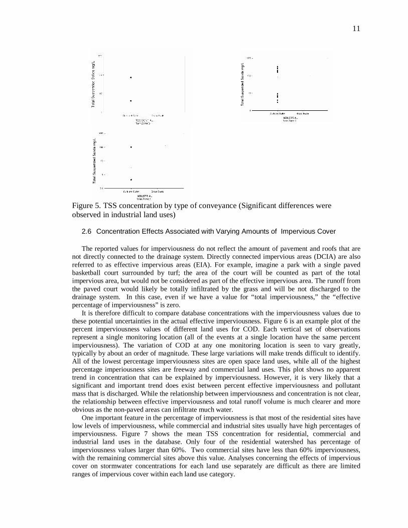
Figure 5 shows box and whisker plots for TSS in industrial land uses, EPA Rain Zones 2 and 3 and residential areas in EPA Rain Zone 2. The median concentrations in industrial land uses were smaller in locations where curbs and gutters were used compared to sites having grass swales. The statistical tests did not identify a significant difference between the median concentrations in residential areas in EPA Rain Zone 3 (the residential boxes have much more overlap than for the industrial sites).

11

Figure 5. TSS concentration by type of conveyance (Significant differences were observed in industrial land uses)

2.6 Concentration Effects Associated with Varying Amounts of Impervious Cover

The reported values for imperviousness do not reflect the amount of pavement and roofs that are

not directly connected to the drainage system. Directly connected impervious areas (DCIA) are also referred to as effective impervious areas (EIA). For example, imagine a park with a single paved basketball court surrounded by turf; the area of the court will be counted as part of the total impervious area, but would not be considered as part of the effective impervious area. The runoff from the paved court would likely be totally infiltrated by the grass and will be not discharged to the drainage system. In this case, even if we have a value for “total imperviousness,” the “effective percentage of imperviousness” is zero.

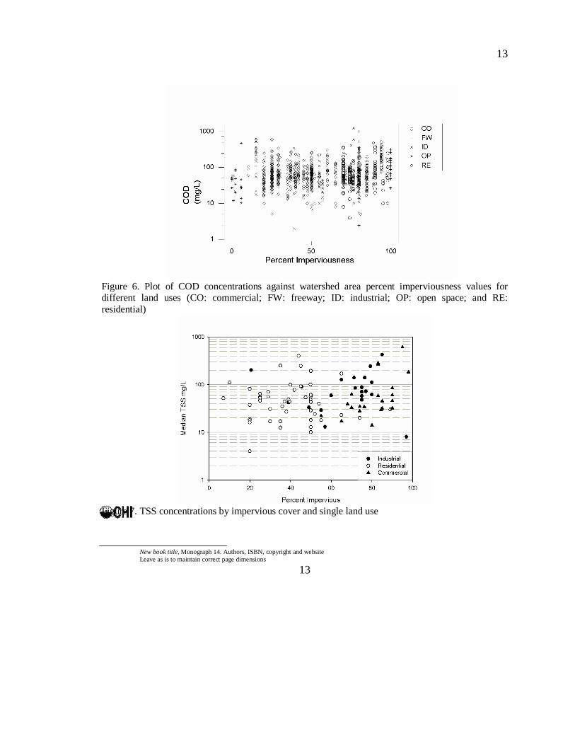
It is therefore difficult to compare database concentrations with the imperviousness values due to these potential uncertainties in the actual effective imperviousness. Figure 6 is an example plot of the percent imperviousness values of different land uses for COD. Each vertical set of observations represent a single monitoring location (all of the events at a single location have the same percent imperviousness). The variation of COD at any one monitoring location is seen to vary greatly, typically by about an order of magnitude. These large variations will make trends difficult to identify. All of the lowest percentage imperviousness sites are open space land uses, while all of the highest percentage imperiousness sites are freeway and commercial land uses. This plot shows no apparent trend in concentration that can be explained by imperviousness. However, it is very likely that a significant and important trend does exist between percent effective imperviousness and pollutant mass that is discharged. While the relationship between imperviousness and concentration is not clear, the relationship between effective imperviousness and total runoff volume is much clearer and more obvious as the non-paved areas can infiltrate much water.

One important feature in the percentage of imperviousness is that most of the residential sites have low levels of imperviousness, while commercial and industrial sites usually have high percentages of imperviousness. Figure 7 shows the mean TSS concentration for residential, commercial and industrial land uses in the database. Only four of the residential watershed has percentage of imperviousness values larger than 60%. Two commercial sites have less than 60% imperviousness, with the remaining commercial sites above this value. Analyses concerning the effects of impervious cover on stormwater concentrations for each land use separately are difficult as there are limited ranges of impervious cover within each land use category.

Tab

le 5

One

-Way

AN

OV

A R

esul

ts b

y T

ype

of C

onve

yanc

e

R

esid

entia

l, E

PA

Rai

n Z

one

2 In

dust

rial,

EP

A R

ain

Zon

e 2

Res

iden

tial,

EP

A R

ain

Zon

e 3

Indu

stria

l, E

PA

Rai

n Z

one

3

Con

stitu

ent

Cur

b an

d G

utte

r

Gra

ss

Sw

ale

p-va

lue

Cur

b an

d G

utte

r

Gra

ss

Sw

ale

p-va

lue

Cur

b an

d G

utte

r

Gra

ss

Sw

ale

p-va

lue

Cur

b an

d G

utte

r

Gra

ss

Sw

ale

p-va

lue

Oil

and

G

reas

e m

g/L

3.11

(59)

2.

95

(7,=

) 0.

824

- -

Non

e -

- N

one

- -

Non

e

TD

S m

g/L

-

- N

one

45.5

(67)

18

4

(77,

>)

0 94

.06

(11)

47

.84

(6,<

) 0.

049

76.7

4 (1

0)

131.

6 (6

,=)

0.13

4

TS

S m

g/L

-

- N

one

37.6

2

(69)

97

.70

(7,>

) 0.

023

19.2

(1

2)

29.6

(6

,=)

0.42

5 9.

68

(10)

91

.2

(6,>

) 0.

014

BO

D m

g/L

-

- N

one

6.84

(67)

39

.98

(5,>

) 0

7.56

(1

1)

6.63

(5

,=)

0.74

9 4.

68

(10)

6.

61

(6,=

) 0.

461

CO

D m

g/L

-

- N

one

50.1

6

(66)

85

.64

(7,>

) 0.

035

29.3

6 (1

1)

67.2

7 (5

,>)

0.02

7 29

.40

(10)

41

.26

(6,=

) 0.

446

Am

mo

nia

m

g/L

-

- N

one

0.22

3

(61)

0.

285

(7,=

) 0.

492

- -

Non

e -

- N

one

NO

2 +

NO

3 m

g/L

-

- N

one

- -

Non

e -

- N

one

- -

Non

e

TK

N m

g/L

-

- N

one

- -

Non

e 1.

22

(11)

0.

94

(6,<

) 0.

170

0.51

5 (9

) 0.

885

(6,=

) 0.

299

Dis

solv

ed

Ph

osp

ho

rus

mg

/L

- -

Non

e 0.

07

(5

0)

0.23

(4

,>)

0.01

2 0.

07

(8)

0.04

(6

,=)

0.32

4 0.

046

(5)

0.02

7 (6

,=)

0.07

7

To

tal

Ph

osp

ho

rus

mg

/L

- -

Non

e 0.

174

(6

4)

0.23

2 (7

,=)

0.46

8 0.

22

(12)

0.

14

(6,=

) 0.

319

0.13

8 (9

) 0.

202

(6,=

) 0.

460

To

tal

Co

pp

er

µg

/L

10.6

7

(82)

3.

11

(7,<

) 0

13

(20)

12

.36

(7,=

) 0.

905

19

(1

1)

5

(6,<

) 0.

007

8.57

(9

) 22

.32

(6,=

) 0.

098

To

tal L

ead

µ

g/L

11

.7

(7

7)

5.67

(7

,=)

0 -

- N

one

12.9

(9

) 4.

20

(6,=

) 0.

154

4.86

(4

) 15

.5

(6,=

) 0.

157

To

tal Z

inc

µg

/L

59.4

6

(82)

17

.85

(7,<

) 0

225.

7

(20)

18

8.4

(7,=

) 0.

447

49.5

(1

1)

43

(6,=

) 0.

781

72.8

6 (9

) 19

8.9

(6,>

) 0.

007

Not

e.

a. T

he

bold

, ita

liciz

ed p

roba

bilit

y va

lues

indi

cat

e “s

tatis

tical

ly s

igni

fica

nt”

findi

ngs

at th

e 0.

05 le

vel

, or

bet

ter.

b. S

am

ple

size

an

d re

sult

from

Dun

net

te

st

com

parin

g if

site

s w

ith g

rass

sw

ale

s pr

oduc

es la

rger

con

cen

tra

tion

s “>

”, s

ma

ller

con

cen

tra

tion

s “<

” or

not

st

atis

tica

lly d

iffer

ence

“=

” th

an s

ites

with

cur

b an

d gu

tters

at a

fam

ily e

rror

of 5

%.“

Non

e” in

dica

tes

no

sa

mpl

es w

ere

colle

cted

for

this

con

stitu

ent i

n th

e gr

oup.

12

13

New book title, Monograph 14. Authors, ISBN, copyright and website Leave as is to maintain correct page dimensions

13

Figure 6. Plot of COD concentrations against watershed area percent imperviousness values for different land uses (CO: commercial; FW: freeway; ID: industrial; OP: open space; and RE: residential)

Figure 7. TSS concentrations by impervious cover and single land use

Leave header as is so vertical dimension of page remains correct 14

Leave footer as is so vertical dimension of page remains correct

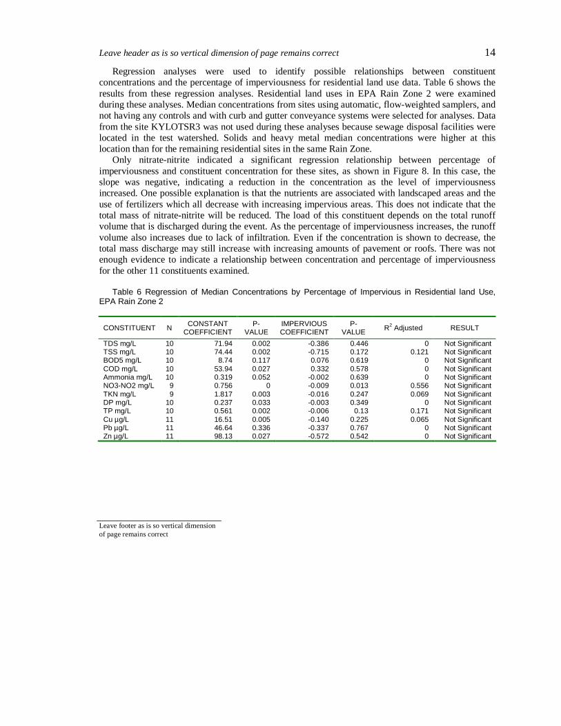
Regression analyses were used to identify possible relationships between constituent concentrations and the percentage of imperviousness for residential land use data. Table 6 shows the results from these regression analyses. Residential land uses in EPA Rain Zone 2 were examined during these analyses. Median concentrations from sites using automatic, flow-weighted samplers, and not having any controls and with curb and gutter conveyance systems were selected for analyses. Data from the site KYLOTSR3 was not used during these analyses because sewage disposal facilities were located in the test watershed. Solids and heavy metal median concentrations were higher at this location than for the remaining residential sites in the same Rain Zone.

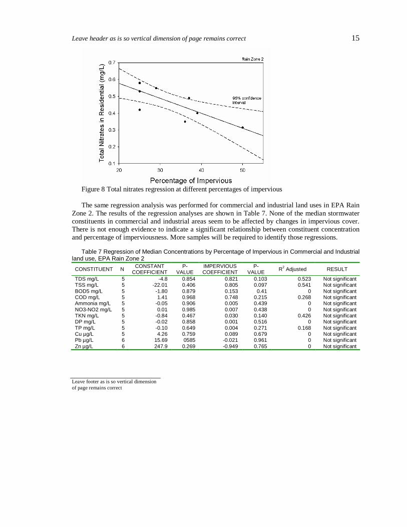
Only nitrate-nitrite indicated a significant regression relationship between percentage of imperviousness and constituent concentration for these sites, as shown in Figure 8. In this case, the slope was negative, indicating a reduction in the concentration as the level of imperviousness increased. One possible explanation is that the nutrients are associated with landscaped areas and the use of fertilizers which all decrease with increasing impervious areas. This does not indicate that the total mass of nitrate-nitrite will be reduced. The load of this constituent depends on the total runoff volume that is discharged during the event. As the percentage of imperviousness increases, the runoff volume also increases due to lack of infiltration. Even if the concentration is shown to decrease, the total mass discharge may still increase with increasing amounts of pavement or roofs. There was not enough evidence to indicate a relationship between concentration and percentage of imperviousness for the other 11 constituents examined.

Table 6 Regression of Median Concentrations by Percentage of Impervious in Residential land Use,

EPA Rain Zone 2

CONSTITUENT N CONSTANT COEFFICIENT

P-VALUE

IMPERVIOUS COEFFICIENT

P-VALUE R2 Adjusted RESULT

TDS mg/L 10 71.94 0.002 -0.386 0.446 0 Not Significant TSS mg/L 10 74.44 0.002 -0.715 0.172 0.121 Not Significant BOD5 mg/L 10 8.74 0.117 0.076 0.619 0 Not Significant COD mg/L 10 53.94 0.027 0.332 0.578 0 Not Significant Ammonia mg/L 10 0.319 0.052 -0.002 0.639 0 Not Significant NO3-NO2 mg/L 9 0.756 0 -0.009 0.013 0.556 Not Significant TKN mg/L 9 1.817 0.003 -0.016 0.247 0.069 Not Significant DP mg/L 10 0.237 0.033 -0.003 0.349 0 Not Significant TP mg/L 10 0.561 0.002 -0.006 0.13 0.171 Not Significant Cu µg/L 11 16.51 0.005 -0.140 0.225 0.065 Not Significant Pb µg/L 11 46.64 0.336 -0.337 0.767 0 Not Significant Zn µg/L 11 98.13 0.027 -0.572 0.542 0 Not Significant



Figure 8 Total nitrates regression at different percentages of impervious The same regression analysis was performed for commercial and industrial land uses in EPA Rain

Zone 2. The results of the regression analyses are shown in Table 7. None of the median stormwater constituents in commercial and industrial areas seem to be affected by changes in impervious cover. There is not enough evidence to indicate a significant relationship between constituent concentration and percentage of imperviousness. More samples will be required to identify those regressions.

Table 7 Regression of Median Concentrations by Percentage of Impervious in Commercial and Industrial

land use, EPA Rain Zone 2


P-VALUE

IMPERVIOUS COEFFICIENT

P-VALUE R2 Adjusted RESULT

TDS mg/L 5 -4.8 0.854 0.821 0.103 0.523 Not significant TSS mg/L 5 -22.01 0.406 0.805 0.097 0.541 Not significant BOD5 mg/L 5 -1.80 0.879 0.153 0.41 0 Not significant COD mg/L 5 1.41 0.968 0.748 0.215 0.268 Not significant Ammonia mg/L 5 -0.05 0.906 0.005 0.439 0 Not significant NO3-NO2 mg/L 5 0.01 0.985 0.007 0.438 0 Not significant TKN mg/L 5 -0.84 0.467 0.030 0.140 0.426 Not significant DP mg/L 5 -0.02 0.858 0.001 0.516 0 Not significant TP mg/L 5 -0.10 0.649 0.004 0.271 0.168 Not significant Cu µg/L 5 4.26 0.759 0.089 0.679 0 Not significant Pb µg/L 6 15.69 0585 -0.021 0.961 0 Not significant Zn µg/L 6 247.9 0.269 -0.949 0.765 0 Not significant



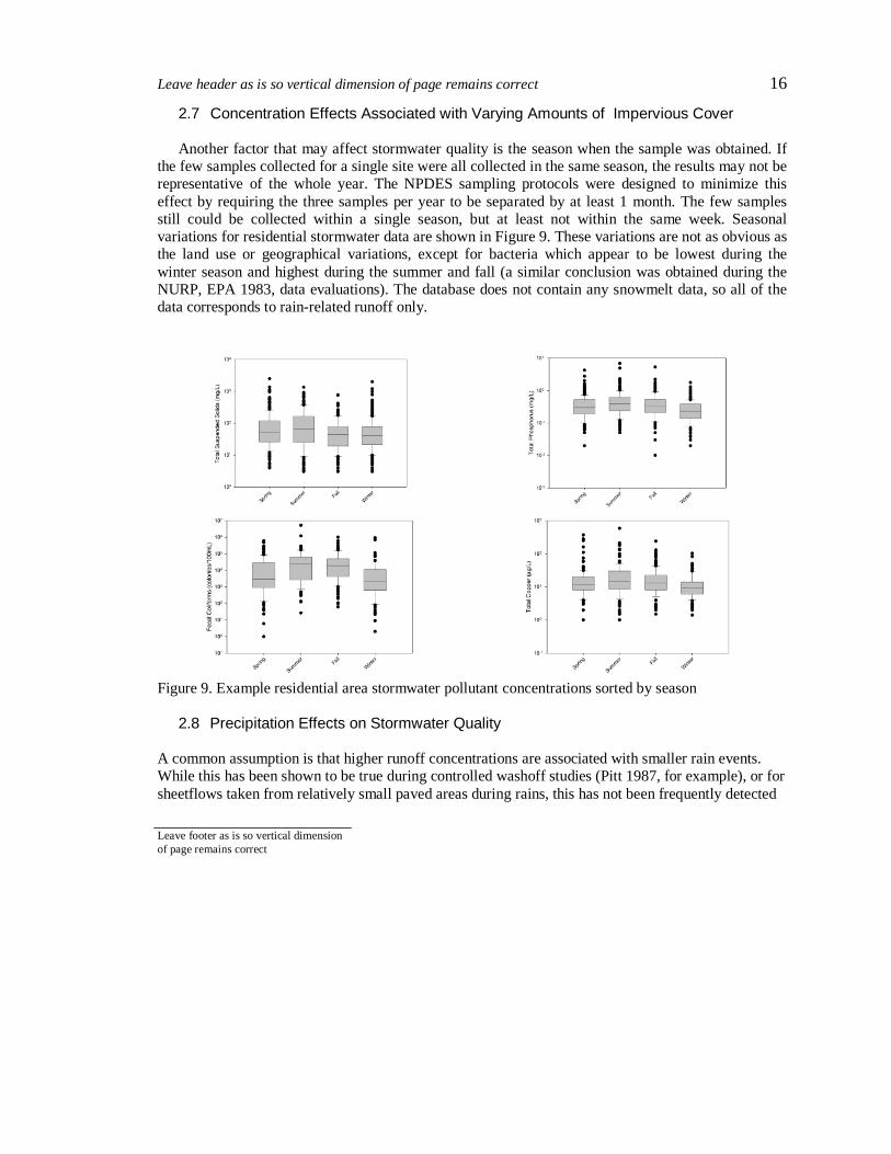
2.7 Concentration Effects Associated with Varying Amounts of Impervious Cover Another factor that may affect stormwater quality is the season when the sample was obtained. If

the few samples collected for a single site were all collected in the same season, the results may not be representative of the whole year. The NPDES sampling protocols were designed to minimize this effect by requiring the three samples per year to be separated by at least 1 month. The few samples still could be collected within a single season, but at least not within the same week. Seasonal variations for residential stormwater data are shown in Figure 9. These variations are not as obvious as the land use or geographical variations, except for bacteria which appear to be lowest during the winter season and highest during the summer and fall (a similar conclusion was obtained during the NURP, EPA 1983, data evaluations). The database does not contain any snowmelt data, so all of the data corresponds to rain-related runoff only.

Figure 9. Example residential area stormwater pollutant concentrations sorted by season

2.8 Precipitation Effects on Stormwater Quality

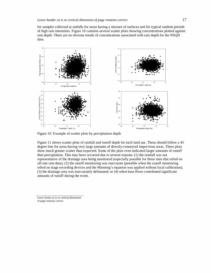
A common assumption is that higher runoff concentrations are associated with smaller rain events. While this has been shown to be true during controlled washoff studies (Pitt 1987, for example), or for sheetflows taken from relatively small paved areas during rains, this has not been frequently detected



for samples collected at outfalls for areas having a mixture of surfaces and for typical random periods of high rain intensities. Figure 10 contains several scatter plots showing concentrations plotted against rain depth. There are no obvious trends of concentrations associated with rain depth for the NSQD data.

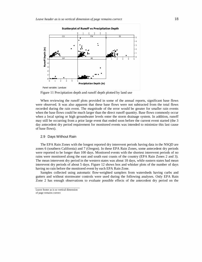
Figure 10. Example of scatter plots by precipitation depth Figure 11 shows scatter plots of rainfall and runoff depth for each land use. These should follow a 45 degree line for areas having very large amounts of directly-connected impervious areas. These plots show much greater scatter than expected. Some of the plots even indicated larger amounts of runoff than precipitation. This may have occurred due to several reasons: (1) the rainfall was not representative of the drainage area being monitored (especially possible for those sites that relied on off-site rain data); (2) the runoff monitoring was inaccurate (possible when the runoff monitoring relied on stage recording devices and the Manning’s equation was applied without local calibration); (3) the drainage area was inaccurately delineated; or (4) when base flows contributed significant amounts of runoff during the event.



Precipitation Depth (in)

Runoff

Depth

(in

)

543210

543210

5

4

3

2

1

0

543210

5

4

3

2

1

0

CO FW ID

OP RE

Panel variable: Landuse

Scatterplot of Runoff vs Precipitation Depth

Figure 11 Precipitation depth and runoff depth plotted by land use When reviewing the runoff plots provided in some of the annual reports, significant base flows

were observed. It was also apparent that these base flows were not subtracted from the total flows recorded during the rain event. The magnitude of the error would be greater for smaller rain events when the base flows could be much larger than the direct runoff quantity. Base flows commonly occur when a local spring or high groundwater levels enter the storm drainage system. In addition, runoff may still be occurring from a prior large event that ended soon before the current event started (the 3 day antecedent dry period requirement for monitored events was intended to minimize this last cause of base flows).

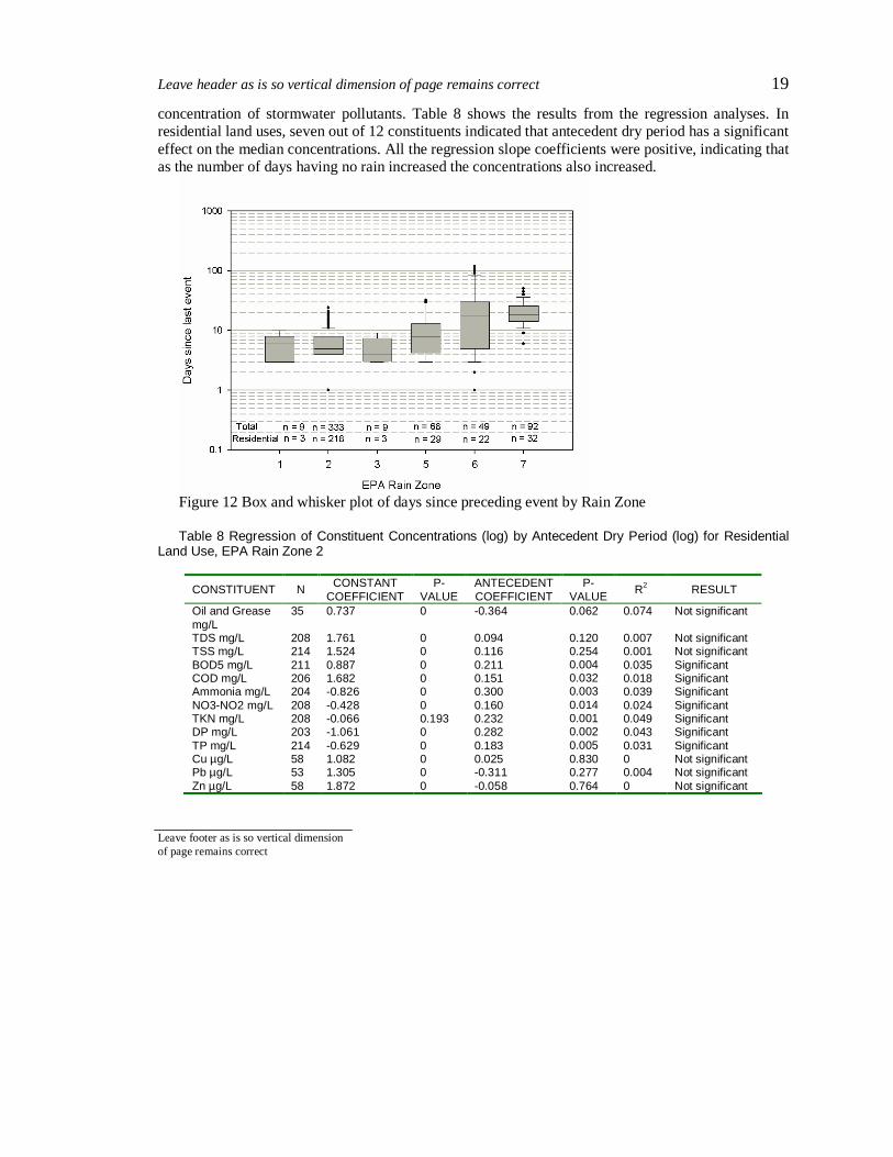
2.9 Days Without Rain The EPA Rain Zones with the longest reported dry interevent periods having data in the NSQD are

zones 6 (southern California) and 7 (Oregon). In these EPA Rain Zones, some antecedent dry periods were reported to be longer than 100 days. Monitored events with the shortest interevent periods of no rains were monitored along the east and south east coasts of the country (EPA Rain Zones 2 and 3). The mean interevent dry period in the western states was about 18 days, while eastern states had mean interevent dry periods of about 5 days. Figure 12 shows box and whisker plots of the number of days having no rain before the monitored event by each EPA Rain Zone.

Samples collected using automatic flow-weighted samplers from watersheds having curbs and gutters and without stormwater controls were used during the following analyses. Only EPA Rain Zone 2 has enough observations to evaluate possible effects of the antecedent dry period on the



concentration of stormwater pollutants. Table 8 shows the results from the regression analyses. In residential land uses, seven out of 12 constituents indicated that antecedent dry period has a significant effect on the median concentrations. All the regression slope coefficients were positive, indicating that as the number of days having no rain increased the concentrations also increased.

Figure 12 Box and whisker plot of days since preceding event by Rain Zone Table 8 Regression of Constituent Concentrations (log) by Antecedent Dry Period (log) for Residential

Land Use, EPA Rain Zone 2


P-VALUE

ANTECEDENT COEFFICIENT

P-VALUE

R2 RESULT

Oil and Grease mg/L

35 0.737 0 -0.364 0.062 0.074 Not significant

TDS mg/L 208 1.761 0 0.094 0.120 0.007 Not significant TSS mg/L 214 1.524 0 0.116 0.254 0.001 Not significant BOD5 mg/L 211 0.887 0 0.211 0.004 0.035 Significant COD mg/L 206 1.682 0 0.151 0.032 0.018 Significant Ammonia mg/L 204 -0.826 0 0.300 0.003 0.039 Significant NO3-NO2 mg/L 208 -0.428 0 0.160 0.014 0.024 Significant TKN mg/L 208 -0.066 0.193 0.232 0.001 0.049 Significant DP mg/L 203 -1.061 0 0.282 0.002 0.043 Significant TP mg/L 214 -0.629 0 0.183 0.005 0.031 Significant Cu µg/L 58 1.082 0 0.025 0.830 0 Not significant Pb µg/L 53 1.305 0 -0.311 0.277 0.004 Not significant Zn µg/L 58 1.872 0 -0.058 0.764 0 Not significant



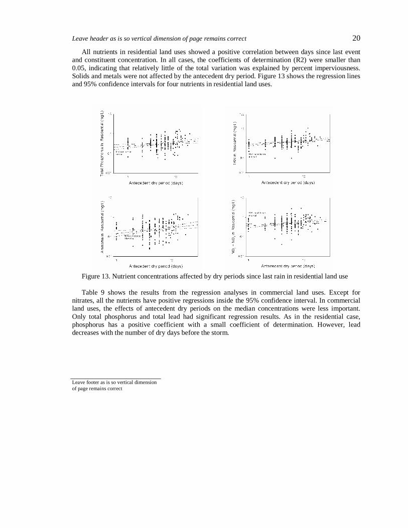
All nutrients in residential land uses showed a positive correlation between days since last event and constituent concentration. In all cases, the coefficients of determination (R2) were smaller than 0.05, indicating that relatively little of the total variation was explained by percent imperviousness. Solids and metals were not affected by the antecedent dry period. Figure 13 shows the regression lines and 95% confidence intervals for four nutrients in residential land uses.

Figure 13. Nutrient concentrations affected by dry periods since last rain in residential land use Table 9 shows the results from the regression analyses in commercial land uses. Except for

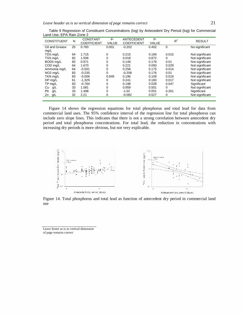
nitrates, all the nutrients have positive regressions inside the 95% confidence interval. In commercial land uses, the effects of antecedent dry periods on the median concentrations were less important. Only total phosphorus and total lead had significant regression results. As in the residential case, phosphorus has a positive coefficient with a small coefficient of determination. However, lead decreases with the number of dry days before the storm.



Table 9 Regression of Constituent Concentrations (log) by Antecedent Dry Period (log) for Commercial Land Use, EPA Rain Zone 2


P-VALUE


P-VALUE

R2 RESULT

Oil and Grease mg/L

25 0.783 0.001 -0.202 0.402 0 No significant

TDS mg/L 64 1.715 0 0.215 0.169 0.015 Not significant TSS mg/L 82 1.506 0 0.018 0.872 0 Not significant BOD5 mg/L 83 0.971 0 0.149 0.176 0.01 Not significant COD mg/L 64 1.670 0 0.221 0.093 0.029 Not significant Ammonia mg/L 64 -0.591 0 0.258 0.175 0.014 Not significant NO2 mg/L 83 -0.235 0 -0.208 0.176 0.01 Not significant TKN mg/L 83 -0.006 0.949 0.196 0.109 0.019 Not significant DP mg/L 61 -1.329 0 0.241 0.160 0.017 Not significant TP mg/L 83 -0.784 0 0.198 0.028 0.047 Significant Cu �g/L 33 1.081 0 0.959 0.501 0 Not significant Pb �g/L 33 1.498 0 -1.02 0.001 0.261 Significant Zn �g/L 32 2.21 0 -0.082 0.527 0 Not significant

Figure 14 shows the regression equations for total phosphorus and total lead for data from

commercial land uses. The 95% confidence interval of the regression line for total phosphorus can include zero slope lines. This indicates that there is not a strong correlation between antecedent dry period and total phosphorus concentrations. For total lead, the reduction in concentrations with increasing dry periods is more obvious, but not very explicable.

Figure 14. Total phosphorus and total lead as function of antecedent dry period in commercial land use



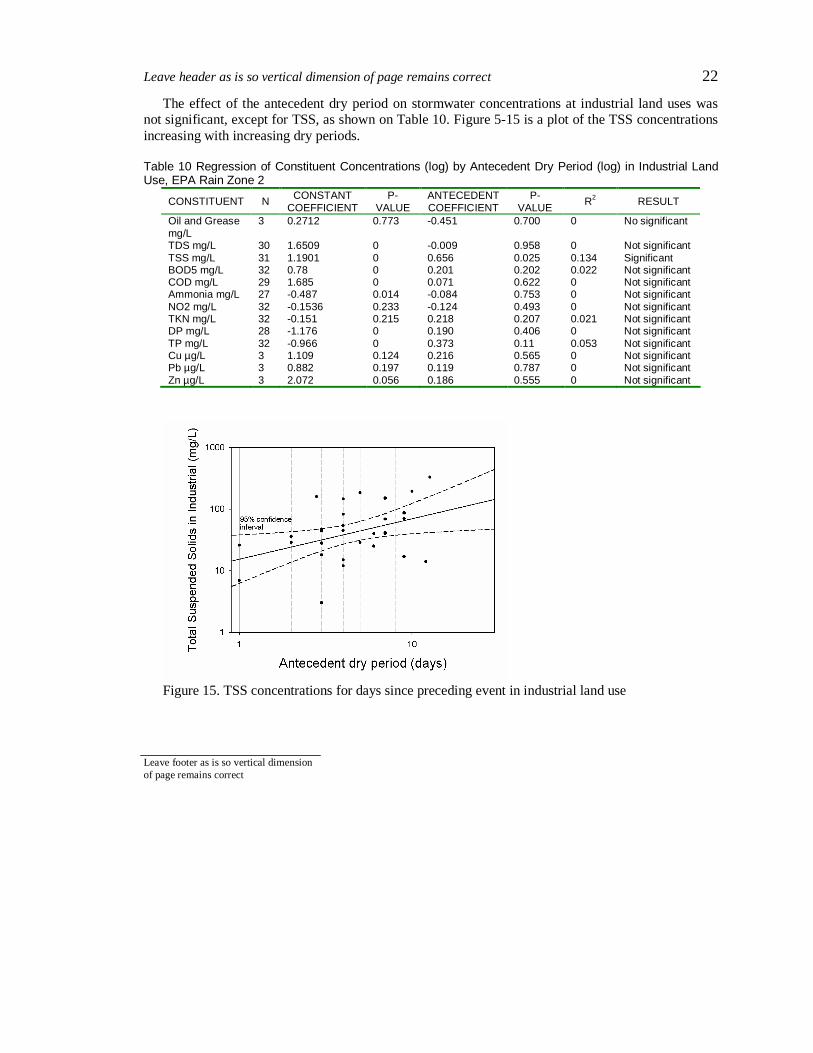
The effect of the antecedent dry period on stormwater concentrations at industrial land uses was not significant, except for TSS, as shown on Table 10. Figure 5-15 is a plot of the TSS concentrations increasing with increasing dry periods.

Table 10 Regression of Constituent Concentrations (log) by Antecedent Dry Period (log) in Industrial Land Use, EPA Rain Zone 2


P-VALUE


P-VALUE

R2 RESULT

Oil and Grease mg/L

3 0.2712 0.773 -0.451 0.700 0 No significant

TDS mg/L 30 1.6509 0 -0.009 0.958 0 Not significant TSS mg/L 31 1.1901 0 0.656 0.025 0.134 Significant BOD5 mg/L 32 0.78 0 0.201 0.202 0.022 Not significant COD mg/L 29 1.685 0 0.071 0.622 0 Not significant Ammonia mg/L 27 -0.487 0.014 -0.084 0.753 0 Not significant NO2 mg/L 32 -0.1536 0.233 -0.124 0.493 0 Not significant TKN mg/L 32 -0.151 0.215 0.218 0.207 0.021 Not significant DP mg/L 28 -1.176 0 0.190 0.406 0 Not significant TP mg/L 32 -0.966 0 0.373 0.11 0.053 Not significant Cu µg/L 3 1.109 0.124 0.216 0.565 0 Not significant Pb µg/L 3 0.882 0.197 0.119 0.787 0 Not significant Zn µg/L 3 2.072 0.056 0.186 0.555 0 Not significant

Figure 15. TSS concentrations for days since preceding event in industrial land use



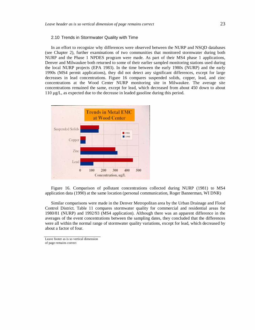
2.10 Trends in Stormwater Quality with Time In an effort to recognize why differences were observed between the NURP and NSQD databases

(see Chapter 2), further examinations of two communities that monitored stormwater during both NURP and the Phase 1 NPDES program were made. As part of their MS4 phase 1 applications, Denver and Milwaukee both returned to some of their earlier sampled monitoring stations used during the local NURP projects (EPA 1983). In the time between the early 1980s (NURP) and the early 1990s (MS4 permit applications), they did not detect any significant differences, except for large decreases in lead concentrations. Figure 16 compares suspended solids, copper, lead, and zinc concentrations at the Wood Center NURP monitoring site in Milwaukee. The average site concentrations remained the same, except for lead, which decreased from about 450 down to about 110 µg/L, as expected due to the decrease in leaded gasoline during this period.

Figure 16. Comparison of pollutant concentrations collected during NURP (1981) to MS4

application data (1990) at the same location (personal communication, Roger Bannerman, WI DNR) Similar comparisons were made in the Denver Metropolitan area by the Urban Drainage and Flood

Control District. Table 11 compares stormwater quality for commercial and residential areas for 1980/81 (NURP) and 1992/93 (MS4 application). Although there was an apparent difference in the averages of the event concentrations between the sampling dates, they concluded that the differences were all within the normal range of stormwater quality variations, except for lead, which decreased by about a factor of four.



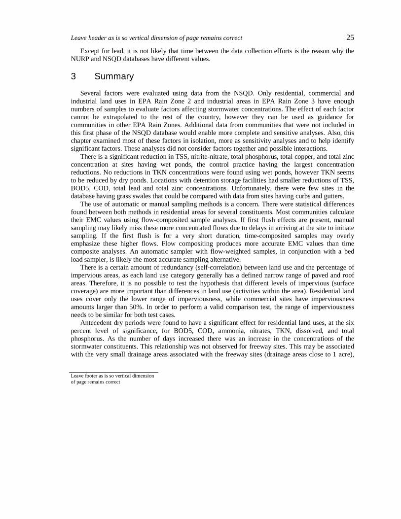
Trends of stormwater concentrations with time can also be examined using the NSQD data. A classical example would be for lead, which is expected to decrease over time with the increased use of unleaded gasoline. Older stormwater samples from the 1970s typically have had lead concentrations of about 100 to 500µg/L, or higher (as indicated above for Milwaukee and Denver), while most current data indicate concentrations as low as 1 to 10 µg/L.

Table 11. Comparison of Commercial and Residential Stormwater Runoff Quality from 1980/81 to 1992/93 (Doerfer, 1993)

CONSTITUENT COMMERCIAL 1980-1981

COMMERCIAL 1992-1993

RESIDENTIAL 1980-1981

RESIDENTIAL 1992-1993

Total suspended solids (mg/L) 251 165 226 325 Total nitrogen (mg/L) 3.0 3.9 3.2 4.7 Nitrate plus nitrite (mg/L) 0.80 1.4 0.61 0.92 Total phosphorus (mg/L) 0.46 0.34 0.61 0.87 Dissolved phosphorus (mg/L) 0.15 0.15 0.22 0.24 Copper, total recoverable (µg/L) 27 81 28 31 Lead, total recoverable (µg/L) 200 59 190 53 Zinc, total recoverable (µg/L) 220 290 180 180

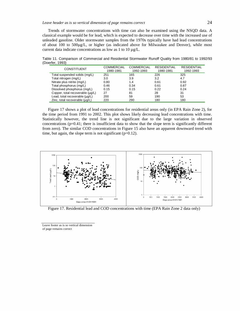
Figure 17 shows a plot of lead concentrations for residential areas only (in EPA Rain Zone 2), for

the time period from 1991 to 2002. This plot shows likely decreasing lead concentrations with time. Statistically however, the trend line is not significant due to the large variation in observed concentrations (p=0.41; there is insufficient data to show that the slope term is significantly different from zero). The similar COD concentrations in Figure 15 also have an apparent downward trend with time, but again, the slope term is not significant (p=0.12).

Figure 17. Residential lead and COD concentrations with time (EPA Rain Zone 2 data only)



Except for lead, it is not likely that time between the data collection efforts is the reason why the NURP and NSQD databases have different values.

3 Summary Several factors were evaluated using data from the NSQD. Only residential, commercial and

industrial land uses in EPA Rain Zone 2 and industrial areas in EPA Rain Zone 3 have enough numbers of samples to evaluate factors affecting stormwater concentrations. The effect of each factor cannot be extrapolated to the rest of the country, however they can be used as guidance for communities in other EPA Rain Zones. Additional data from communities that were not included in this first phase of the NSQD database would enable more complete and sensitive analyses. Also, this chapter examined most of these factors in isolation, more as sensitivity analyses and to help identify significant factors. These analyses did not consider factors together and possible interactions.

There is a significant reduction in TSS, nitrite-nitrate, total phosphorus, total copper, and total zinc concentration at sites having wet ponds, the control practice having the largest concentration reductions. No reductions in TKN concentrations were found using wet ponds, however TKN seems to be reduced by dry ponds. Locations with detention storage facilities had smaller reductions of TSS, BOD5, COD, total lead and total zinc concentrations. Unfortunately, there were few sites in the database having grass swales that could be compared with data from sites having curbs and gutters.

The use of automatic or manual sampling methods is a concern. There were statistical differences found between both methods in residential areas for several constituents. Most communities calculate their EMC values using flow-composited sample analyses. If first flush effects are present, manual sampling may likely miss these more concentrated flows due to delays in arriving at the site to initiate sampling. If the first flush is for a very short duration, time-composited samples may overly emphasize these higher flows. Flow compositing produces more accurate EMC values than time composite analyses. An automatic sampler with flow-weighted samples, in conjunction with a bed load sampler, is likely the most accurate sampling alternative.

There is a certain amount of redundancy (self-correlation) between land use and the percentage of impervious areas, as each land use category generally has a defined narrow range of paved and roof areas. Therefore, it is no possible to test the hypothesis that different levels of impervious (surface coverage) are more important than differences in land use (activities within the area). Residential land uses cover only the lower range of imperviousness, while commercial sites have imperviousness amounts larger than 50%. In order to perform a valid comparison test, the range of imperviousness needs to be similar for both test cases.

Antecedent dry periods were found to have a significant effect for residential land uses, at the six percent level of significance, for BOD5, COD, ammonia, nitrates, TKN, dissolved, and total phosphorus. As the number of days increased there was an increase in the concentrations of the stormwater constituents. This relationship was not observed for freeway sites. This may be associated with the very small drainage areas associated with the freeway sites (drainage areas close to 1 acre),



while the drainage areas for residential, commercial and industrial areas ranged between 50 and 100 acres (Figure2.2).

No seasonal effects on concentrations were observed, except for bacteria levels that appear to be lower in winter and high in summer. No effects on concentration were observed according to precipitation depth. Rainfall energy determines erosion and washoff of particulates, but sufficient runoff volume is needed to carry the particulate pollutants to the outfalls. Different travel times from different locations in the drainage areas results in these materials arriving at different times, plus periods of high rainfall intensity occur randomly throughout the storm. The resulting outfall stormwater concentration patterns for a large area having various surfaces is therefore complex and rain depth is just one of the factors involved.

4 References American Society of Civil Engineers (ASCE), United States Environmental Protection Agency (EPA). 2000.

Determining Urban Stormwater Best Management Practice (BMP) Removal Efficiencies. Task 3.4 Final Data Exploration and Evaluation Report. Office of Water. Washington D.C.

American Society of Civil Engineers (ASCE), United States Environmental Protection Agency (EPA). 2002. Urban

Stormwater BMP Performance Monitoring. A Guidance Manual for Meeting the National Stormwater BMP Database Requirements. Office of Water. Washington D.C. EPA

Arnorld C., Gibbons J. 1996. Impervious Surface Coverage. The Emergency of a Key Environmental Indicator. Journal

of the American Planning Association (62) : 243-58 American Public Health Association (APHA), American Water Works Association (AWWA), and Water Environment

Federation (WEF). 1995. Standard Methods for the Examination of Water and Wastewater. 19th edition. EPS Group Inc

Bailey R. 1993. Using Automatic Samplers to comply with stormwater regulations. Water Engineering and

Management. In: Water Engineering and Management (140) : 23 – 25. Bannerman R., Owens D., Dodds R., Hornewer N. 1993. Source of Pollutants in Wisconsin Stormwater. Water Science

and Technology. (28) : 241-59 Berthouex P., Brown L. 2002. Statistics for Environmental Engineers. Boca Raton, Florida : Lewis Publishers. Burton A., Pitt R. 2002. Stormwater Effects Handbook. A Toolbox for Watershed Managers, Scientists, and Engineers.

Boca Raton, Florida : Lewis Publishers. Driver, N.E., Mustard, M.H., Rhinesmith, R.B., and Middleburg, R.F. 1985. U.S. Geological Survey Urban Stormwater

Database for 22 Metropolitan Areas Throughout the United States. U.S. Geological Survey Open File Report 85-337. Denver, CO: USGS



Doerfer J., Urbonas B. 1993. Stormwater Quality Characterization in the Denver Metropolitan Area. In: Flood Hazard

News 23 (1): 21 - 3 Gibbons J., Chakraborti S. 2003. Nonparametric Statistical Inference. New York, NY: Marcel Dekker Inc. Kottegoda N.T. and Rosso R. 1998. Statistics, Probability and Reliability for Civil and Environmental Engineers. New

York, NY: WCB McGraw-Hill. Leecaster M., Schiff K., Tiefenthaler L. 2002. Assessment of efficient sampling designs for urban stormwater

monitoring. Water Research (36): 1556 – 64 Maestre A., Pitt R., Williamson D. 2004. Nonparametric Statistical Test Comparing First Flush and Composite

Samples from the National Stormwater Quality Database. In: Innovative Modeling of Urban Water Systems. Monograph 12 (James W. Ed.) Guelph, Ontario: Computational Hydraulics International: CHI.

Maestre A., Pitt R., Durrans S. R., Chakraborti S. 2005a. Stormwater Quality Descriptions Using the Three Parameter

Lognormal Distribution. In: Effective Modeling of Urban Water Systems. Monograph 13 (James W. Ed.) Guelph, Ontario: Computational Hydraulics International: CHI.

Maestre A. 2005b. Stormwater Characteristics as Described in the National Stormwater Quality Database. Ph.D.

Dissertation. Department of Civil and Environmental Engineering, University of Alabama. Tuscaloosa, Alabama. National Council of the Paper Industry for Air and Stream Improvement (NCASI). 1995. A Statistical Method and

Computer Program for Estimating the Mean and Variance of Multi-level Left Censored Data Sets. Technical Bulletin No. 703.

Nara Y., Pitt R., Durrans R., Kirby J. (Forthcoming 2006). The Use of Grass Swales as a Stormwater Control. In:

Stormwater and Urban Water System Modeling (James W. Ed.) Guelph, Ontario: Computational Hydraulics International: CHI.

Pitt R., and McLean J. 1986a. Toronto Area Watershed Management Strategy Study. Humber River Pilot Watershed Project. Ontario Ministry of the Environment, Toronto, Ontario. Pitt R. 1986b. The Incorporation of Urban Runoff Controls in the Wisconsin Priority Watershed Program. In:

Advanced Topics in Urban Runoff Research (Urbonas B., Roesner L.A. Ed.). Engineering Foundation and ASCE. New York NY: 290-313

Pitt R. 1987. Small Storm Urban Flow and Particulate Washoff Contributions to Outfall Discharges. Ph.D. Dissertation.

Department of Civil and Environmental Engineering, University of Wisconsin. Madison, Wisconsin. Pitt R., Voorhees J. 1995. Source Loading and Management Model (SLAMM). In: Seminar Watershed Management at

the local, County, and State Levels. Center for Environmental Research Information. United States Environmental Protection Agency EPA: EPA/625/R-95/003. Cincinnati, Ohio

Pitt R., Lilburn M., Durrans S.R., Burian S., Nix S., Voorhees J., and Martinson J. 1999.



Guidance Manual for Integrated Wet Weather Flow (WWF) Collection and Treatments Systems for Newly Urbanized Areas. U.S. Environmental Protection Agency.

Pitt, R., Maestre A., and Morquecho R. 2003. Evaluation of NPDES Phase I Municipal Stormwater Monitoring Data.

In: National Conference on Urban Stormwater: Enhancing the Programs at the Local Level. EPA/625/R-03/003 Pitt, R., Maestre A., Morquecho R., and Williamson D. 2004. Collection and Examination of a Municipal Separate

Storm Sewer System Database. In: Innovative Modeling of Urban Water Systems. Monograph 12 (James W. Ed.) Guelph, Ontario: Computational Hydraulics International: CHI.

Roa-Espinosa A., Bannerman R. 1995. Monitoring BMP effectiveness at industrial sites. In: Conference on Stormwater

NPDES Related Monitoring Needs. ASCE: 467-486. Schueler T., Galli J. 1995. The Environmental Impacts of Stormwater Ponds. In: Stormwater Runoff and Receiving

Systems: Impact, Monitoring and Assessment (CRC Lewis Publishers), Boca Raton, Florida, 177-191. Smullen, J.T. and Cave K.A. 2002. National Stormwater Runoff Pollution Database. In: Wet-Weather Flow in the

Urban Watershed (Field, R., and D. Sullivan. Ed.). Boca Raton, Florida: Lewis Publishers. United States Environmental Protection Agency (EPA). 1983. Results of the Nationwide Runoff Program. Water

Planning Division, PB 84-185552. Washington D.C: EPA United States Environmental Protection Agency (EPA). 1986. Methodology for Analysis of Detention Basins for

Control of Urban Runoff Quality. Office of Water, Nonpoint Source Division. Washington D.C: EPA Van Buren M., Watt A., Marsalek J. 1997. Application of the Lognormal and Normal Distribution to Stormwater

Quality Parameters. Water Research 31 (1): 95 - 104

identification of significant factors affecting stormwater...

Documents