Identical phase oscillators with global sinusoidal coupling evolve by Möbius groupactionSeth A. Marvel, Renato E. Mirollo, and Steven H. Strogatz

Citation: Chaos: An Interdisciplinary Journal of Nonlinear Science 19, 043104 (2009); doi: 10.1063/1.3247089 View online: http://dx.doi.org/10.1063/1.3247089 View Table of Contents: http://scitation.aip.org/content/aip/journal/chaos/19/4?ver=pdfcov Published by the AIP Publishing Articles you may be interested in Networked dynamical systems with linear coupling: Synchronisation patterns, coherence and otherbehaviours Chaos 23, 043112 (2013); 10.1063/1.4826697 Phase synchronization between collective rhythms of globally coupled oscillator groups: Noisy identical case Chaos 20, 043109 (2010); 10.1063/1.3491344 Low dimensional behavior of large systems of globally coupled oscillators Chaos 18, 037113 (2008); 10.1063/1.2930766 Phase Transitions in Globally Coupled Systems AIP Conf. Proc. 795, 202 (2005); 10.1063/1.2128337 Noise enhanced phase synchronization and coherence resonance in sets of chaotic oscillators with weakglobal coupling Chaos 13, 267 (2003); 10.1063/1.1513081

This article is copyrighted as indicated in the article. Reuse of AIP content is subject to the terms at: http://scitation.aip.org/termsconditions. Downloaded to IP:

136.167.54.43 On: Fri, 18 Jul 2014 18:13:31

Identical phase oscillators with global sinusoidal coupling evolveby Möbius group action

Seth A. Marvel,1,a� Renato E. Mirollo,2 and Steven H. Strogatz1

1Center for Applied Mathematics, Cornell University, Ithaca, New York 14853, USA2Department of Mathematics, Boston College, Chestnut Hill, Massachusetts 02167, USA

�Received 23 July 2009; accepted 21 September 2009; published online 15 October 2009�

Systems of N identical phase oscillators with global sinusoidal coupling are known to displaylow-dimensional dynamics. Although this phenomenon was first observed about 20 years ago, itsunderlying cause has remained a puzzle. Here we expose the structure working behind the scenes ofthese systems by proving that the governing equations are generated by the action of the Möbiusgroup, a three-parameter subgroup of fractional linear transformations that map the unit disk toitself. When there are no auxiliary state variables, the group action partitions the N-dimensionalstate space into three-dimensional invariant manifolds �the group orbits�. The N−3 constants ofmotion associated with this foliation are the N−3 functionally independent cross ratios of theoscillator phases. No further reduction is possible, in general; numerical experiments on models ofJosephson junction arrays suggest that the invariant manifolds often contain three-dimensionalregions of neutrally stable chaos. © 2009 American Institute of Physics. �doi:10.1063/1.3247089�

Large arrays of coupled limit-cycle oscillators have beenused to model diverse systems in physics, biology, chem-istry, engineering, and social science. The special case ofphase oscillators coupled all to all through sinusoidal in-teractions has attracted mathematical interest because ofits analytical tractability. About 20 years ago, numericalexperiments revealed that when the oscillators are allidentical, these systems display an exceptionally simpleform of collective behavior: For all N�3, where N is thenumber of oscillators, all trajectories are confined tomanifolds with N−3 fewer dimensions than the statespace itself. Several insights have been obtained over thepast two decades, but it has remained an open problem topinpoint the symmetry or other structure that causes thisnongeneric behavior. Here we show that group theoryprovides the explanation: The governing equations forthese systems arise naturally from the action of the groupof conformal mappings of the unit disk to itself. This linkunifies and explains the previous numerical and analyti-cal results, and yields new constants of motion for thisclass of dynamical systems.

I. INTRODUCTION

When a nonlinear system shows unexpectedly simplebehavior, it may be a clue that some hidden structure awaitsdiscovery. For example, recall the classic detective story1

that began in the 1950s with the work of Fermi, Pasta, andUlam.2–4 In their numerical simulations of a chain of anhar-monic oscillators, Fermi et al. were surprised to find thechain returning almost perfectly, again and again, to its initialstate. The struggle to understand these recurrences ledZabusky and Kruskal5 to the discovery of solitons in theKorteweg–deVries equation, which in turn sparked a series

of results showing that this equation possessed many con-served quantities—in fact, infinitely many.6 Then severalother equations turned out to have the same properties. At thetime these results seemed almost miraculous. But by themid-1970s the hidden structure responsible for all of them—the complete integrability of certain infinite-dimensionalHamiltonian systems7—had been made manifest by the in-verse scattering transform8,9 and Lax10 pairs.

Something similar, although far less profound, has beenhappening again in nonlinear science. The broad topic is stillcoupled oscillators, but unlike the conservative oscillatorsstudied by Fermi et al., the oscillators in question now aredissipative and have stable limit cycles. This latest story be-gan around 1990 when a few researchers noticed an enor-mous amount of neutral stability and seemingly low-dimensional behavior in their simulations of Josephsonjunction arrays—specifically, arrays of identical, over-damped junctions arranged in series and coupled through acommon load.11–15 Then, just a year ago, Antonsen et al.16

uncovered similarly low-dimensional dynamics in the peri-odically forced version of the Kuramoto model of biologicaloscillators.17–19 This was particularly surprising because theoscillators in that model are nonidentical.

As in the soliton story, these numerical observations theninspired a series of theoretical advances. For the case ofidentical oscillators �the subject of this paper�, these includedthe discovery of constants of motion20,21 and of a pair oftransformations that established the low dimensionality ofthe dynamics.20–25 But what remained to be found was thefinal piece, the identification of the hidden structure. Withoutit, it was unclear why the transformations and constants ofmotion should exist in the first place.

In this paper we show that the group of Möbius trans-formations is the key to understanding this class of dynami-cal systems. Our analysis unifies the previous treatments ofa�Electronic mail: sam255@cornell.edu.

CHAOS 19, 043104 �2009�

1054-1500/2009/19�4�/043104/11/$25.00 © 2009 American Institute of Physics19, 043104-1

This article is copyrighted as indicated in the article. Reuse of AIP content is subject to the terms at: http://scitation.aip.org/termsconditions. Downloaded to IP:

136.167.54.43 On: Fri, 18 Jul 2014 18:13:31

Josephson arrays and the Kuramoto model, and clarifies thegeometric and algebraic structures responsible for their low-dimensional behavior. One spinoff of our approach is a newset of constants of motion; these generalize the constantsfound previously and hold for a wider class of oscillatorarrays.

The paper is organized as follows. To keep the treatmentself-contained and to establish notation, Sec. II reviews therelevant background about coupled oscillators and theMöbius group. In Sec. III we show how to use Möbius trans-formations to reduce the dynamics of identical oscillatorswith global sinusoidal coupling, the type of coupling thatappears in both the Josephson and Kuramoto models. Thereduced flow lives on a set of invariant three-dimensionalmanifolds, arising naturally as the so-called group orbits ofthe Möbius group. The results obtained in this way are thencompared with previous findings �Sec. IV� and used to gen-erate new constants of motion via the classical cross ratioconstruction �Sec. V�. We explore the dynamics on the in-variant manifolds in Sec. VI and show that the phase por-traits for resistively coupled Josephson arrays are filled withchaos and island chains, reminiscent of the pictures encoun-tered in Hamiltonian chaos and Kolmogorov–Arnold–Mosertheory.

II. BACKGROUND

A. Reducible systems with sinusoidal coupling

The theory developed here was originally motivated bysimulations of the governing equations for a series array of Nidentical, overdamped Josephson junctions driven by a con-stant current and coupled through a resistive load. As shownin Tsang et al.,11 the dimensionless circuit equations for thissystem can be written as

� j = � − �b + 1�cos � j +1

N�k=1

N

cos �k �1�

for j=1, . . . ,N. The physical interpretation need not concernus here; the important point for our purposes is that this setof N ordinary differential equations �ODEs� displayed low-dimensional dynamics. The same sort of low-dimensionalbehavior was later found in other kinds of oscillator arrays14

as well as in Josephson arrays with other kinds ofloads.12,13,15

Building on contributions from several teams ofresearchers,11–15 Watanabe and Strogatz21 showed that thesystem �1� could be reduced from N ODEs to three ODEs inthe following sense. Consider a time-dependent transforma-tion from a set of constant angles � j to a set of functions� j�t� defined via

tan�� j�t� − ��t�2

� =�1 + ��t�1 − ��t�

tan�� j − ��t�2

� �2�

for j=1, . . . ,N. By direct substitution, one can check that theresulting functions � j�t� simultaneously satisfy all N equa-tions in Eq. �1� as long as the three variables ��t�, ��t� and��t� satisfy a certain closed set of ODEs.21

Watanabe and Strogatz also noted that the same transfor-mation can be used to reduce any system of the form

� j = fei�j + g + fe−i�j �3�

for j=1, . . . ,N, where f is any smooth, complex-valued2�-periodic function of the phases �1 , . . . ,�N. �Here theoverbar denotes complex conjugate. Also, note that g has tobe real valued since � j is real.� The functions f and g areallowed to depend on time and on any other auxiliary statevariables in the system, for example, the charge on a loadcapacitor or the current through a load resistor for certainJosephson junction arrays. The key is that f and g must bethe same for all oscillators, and thus do not depend on theindex j. We call such systems sinusoidally coupled becausethe dependence on j occurs solely through the first harmon-ics ei�j and e−i�j.

Soon after the transformation �2� was reported, Goebel22

observed that it could be related to fractional linear transfor-mations, and he used this fact to simplify some of the calcu-lations in Ref. 21. At that point, research on the reducibilityof Josephson arrays paused for more than a decade. Thequestion of why this particular class of dynamical systems�3� should be reducible by fractional linear transformationswas not pursued at that time, but will be addressed inSec. III.

B. Ott–Antonsen ansatz

Ott and Antonsen23,25 recently reopened the issue of low-dimensional dynamics with their discovery of an ansatz thatcollapses the infinite-dimensional Kuramoto model to a two-dimensional system of ODEs.

To illustrate their ansatz in its simplest form, let us applyit to the class of identical oscillators governed by Eq. �3� inthe limit N→. �Note that this step involves two simplifyingassumptions, namely, that N is infinitely large and that theoscillators are identical. The Ott–Antonsen ansatz appliesmore generally to systems of nonidentical oscillators withfrequencies chosen at random from a prescribed probabilitydistribution—indeed, this generalization was one of Ott andAntonsen’s major advances—but it is not needed for the is-sues that we wish to address.� In the limit N→, the evolu-tion of the system �3� is given by the continuity equation

�

�t+

��v���

= 0, �4�

where the phase density �� , t� is defined such that �� , t�d�gives the fraction of phases that lie between � and �+d� attime t, and where the velocity field is the Eulerian version ofEq. �3�,

v��,t� = fei� + g + fe−i�. �5�

Our earlier assumptions about the coefficient functions f andg now take the form that f and g may depend on t but not on�. The time dependence of f and g can arise either explicitly�say, through external forcing� or implicitly �through the timedependence of the harmonics of or any auxiliary state vari-ables in the system�.

Following Ott and Antonsen,23 suppose is of the form

043104-2 Marvel, Mirollo, and Strogatz Chaos 19, 043104 �2009�

This article is copyrighted as indicated in the article. Reuse of AIP content is subject to the terms at: http://scitation.aip.org/termsconditions. Downloaded to IP:

136.167.54.43 On: Fri, 18 Jul 2014 18:13:31

��,t� =1

2�1 + �

n=1

���t�nein� + ��t�ne−in�� �6�

for some unknown function � that is independent of �. �Ourdefinition of � is, however, slightly different from that in Ottand Antonsen;23 our � is their �.� Note that Eq. �6� is just analgebraic rearrangement of the usual form for the Poissonkernel

��� =1

2�

1 − r2

1 − 2r cos�� − �� + r2 , �7�

where r and � are defined via

� = rei�. �8�

In geometrical terms, the ansatz �6� defines a submanifold inthe infinite-dimensional space of density functions . ThisPoisson submanifold is two dimensional and is parametrizedby the complex number �, or equivalently, by the polar co-ordinates r and �.

The intriguing fact discovered by Ott and Antonsen isthat the Poisson submanifold is invariant: If the density isinitially a Poisson kernel, it remains a Poisson kernel for alltime. To verify this, we substitute the velocity field �5� andthe ansatz �6� into the continuity equation �4�, and find thatthe amplitude equations for each harmonic ein� are simulta-neously satisfied if and only if ��t� evolves according to

� = i�f�2 + g� + f� . �9�

This equation can be recast in a more physically mean-ingful form in terms of the complex order parameter denotedby �z� and defined as the centroid of the phases � regarded aspoints ei� on the unit circle:

�z� = 0

2�

ei���,t�d� . �10�

By substituting Eq. �6� into Eq. �10� we find that �z�=� forall states on the Poisson submanifold. Hence, �z� satisfies theRiccati equation

d

dt�z� = i�f�z�2 + g�z� + f� . �11�

When f and g are functions of �z� alone, as in mean-fieldmodels, Eq. �11� constitutes a closed two-dimensional sys-tem for the flow on the Poisson submanifold. More generally,the system will be closed whenever f and g depend on onlythrough its Fourier coefficients. We will show this explicitlyin Sec. V B by finding formulas for all the higher Fouriercoefficients in terms of �, and hence in terms of �z�. �How-ever, as we will see, things become more complicated forstates lying off the Poisson submanifold. Then �z� no longercoincides with � and the closed system becomes three di-mensional involving � as well as �.�

The work of Ott and Antonsen23 raises several questions.Why should the set of Poisson kernels be invariant? What isthe relationship, if any, between the ansatz �6� and the trans-formation equation �2� studied earlier? Why does Eq. �2�

reduce equations of the form �3� to a three-dimensional flow,whereas Eq. �6� reduces them to a two-dimensional flow?

As we shall see, the answers have to do with the prop-erties of the group of conformal mappings of the unit disk toitself. Before showing how this group arises naturally in thedynamics of sinusoidally coupled oscillators, let us recallsome of its relevant properties.

C. Möbius group

Consider the set of all fractional linear transformationsF :C→C of the form

F�z� =az + b

cz + d, �12�

where a, b, c, and d are complex numbers, and the numeratoris not a multiple of the denominator �that is, ad−bc�0�.This family of functions carries the structure of a group. Thegroup operation is composition of functions, the identity el-ement is the identity map, and inverses are given by inversefunctions.

Of most importance to us is a subgroup G—which werefer to as the Möbius group—consisting of those fractionallinear transformations that map the open unit disk D= �z�C : �z� 1� onto itself in a one-to-one way. These transfor-mations and their inverses are analytic on D and map itsboundary �the unit circle S1= �z�C : �z�=1�� to itself. All suchautomorphisms of the disk can be written26 in the form

F�z� = ei� � − z

1 − �z�13�

for some ��R and ��D. The Möbius group G is in fact athree-dimensional Lie group with real parameters �, Re���,and Im���.

However, it turns out that a different parametrization ofG will be more notationally convenient in what follows inthe sense that it simplifies comparisons between our resultsand those in the prior literature. Specifically, we will view atypical element of G as a mapping M from the unit disk inthe complex w-plane to the unit disk in the complex z-planewith parametrization given by

z = M�w� =ei�w + �

1 + �ei�w, �14�

where ��D and ��R. Note that the inverse mapping

w = M−1�z� = e−i� z − �

1 − �z�15�

has an appearance closer to that of the standard parametriza-tion �Eq. �13��.

A word about terminology: our definition of the Möbiusgroup is not the conventional one. Usually this term denotesthe larger group of all fractional linear transformations �orbilinear transformations or linear fractional transformations�,whereas we reserve the adjective Möbius for the subgroup Gand its elements. Thus, from now on, when we say Möbiustransformation we specifically mean an element of the sub-group G consisting of analytic automorphisms of the unitdisk.

043104-3 Phase oscillators and the Möbius group Chaos 19, 043104 �2009�

This article is copyrighted as indicated in the article. Reuse of AIP content is subject to the terms at: http://scitation.aip.org/termsconditions. Downloaded to IP:

136.167.54.43 On: Fri, 18 Jul 2014 18:13:31

III. MÖBIUS GROUP REDUCTION

In this section we show that if the equations for theoscillator array are of the form �3�, then the oscillators’phases � j�t� evolve according to the action of the Möbiusgroup on the complex unit circle

ei�j�t� = Mt�ei�j� �16�

for j=1, . . . ,N, where Mt is a one-parameter family ofMöbius transformations and � j is a constant �time-independent� angle. In other words, the time-t flow map forthe system is always a Möbius map.

Incidentally, this result is consistent with a basic topo-logical fact: We know that different oscillators cannot passthrough each other on S1 under the flow, so we expect thetime-t flow map to be an orientation-preserving homeomor-phism of S1 onto itself—and indeed any Möbius map is.

We begin the analysis with an algebraic method similarto that in Goebel.22 Then, in Secs. III B and III C, we adopta geometrical perspective and show that it answers severalquestions left open by the first method.

A. Algebraic method

Parametrize the one-parameter family of Möbius trans-formations as

Mt�w� =ei�w + �

1 + �ei�w, �17�

where ���t�� 1 and ��t��R, and let

wj = ei�j . �18�

To verify that Eq. �17� gives an exact solution of Eq. �3�—subject to the constraint that the Möbius parameters ��t� and��t� obey appropriate ODEs to be determined—we computethe time derivative of � j�t�=−i log Mt�wj�, keeping in mindthat wj is constant,

� j =�ei�wj − i�

ei�wj + �+

�i� − ���ei�wj

1 + �ei�wj

. �19�

From Eq. �15�, we get

ei�wj =ei�j − �

1 − �ei�j, �20�

which when substituted into Eq. �19� yields

� j = Rei�j +� + i�� − ��i� − ���

1 − ���2+ Re−i�j , �21�

where R= �i�− ��� / �1− ���2�.Note that Eq. �21� falls precisely into the algebraic form

required by Eq. �3�. Thus, to derive the desired ODEs for��t� and ��t�, we now subtract Eq. �21� from Eq. �3� toobtain N equations of the form 0=C1ei�j +C0+C−1e−i�j forj=1, . . . ,N. If the system contains at least three distinct os-cillator phases, then C1, C0, and C−1 must generically bezero. Explicitly,

f =i� − ��

1 − ���2, g =

� + i�� − ��i� − ���1 − ���2

. �22�

The system �22� can be algebraically rearranged to give

� = i�f�2 + g� + f� , �23a�

� = f� + g + f� . �23b�

Equations �23a� and �23b� have been derived previously;they appear as Eqs. �10� and �11�, respectively, in Pikovskyand Rosenblum’s work,24 where they were derived by apply-ing the transformation equation �2�. Both their approach andthe one above are certainly quick and clean, but they requireus to guess the transformation ahead of time, and reveal littleabout why this transformation works.

Incidentally, observe that under the change of variableszj =ei�j, Eq. �3� becomes

z j = i�fzj2 + gzj + f� . �24�

Equation �24� is a Riccati equation with the form of Eq.�23a�—another coincidence that seems a bit surprising whenapproached this way. In Sec. III B, we will see how theseRiccati equations emerge naturally from the infinitesimalgenerators of the Möbius group.

B. Geometric method of finding �

Now we change our view of Möbius maps slightly. In-stead of thinking of M as a map from the w-plane to thez-plane, we view it as a map from the z-plane to itself. Thisrequires a small and temporary change in notation, but itmakes things clearer, especially when we start to discussdifferential equations on the complex plane.

We begin by recalling some basic facts and definitions.Suppose the coupled oscillator system contains just three dis-tinct phases among its N oscillators. Then by a property ofMöbius transformations, there exists a unique Möbius trans-formation from any point z1= �ei�1 ,ei�2 ,ei�3� to any otherpoint z2= �ei�1 ,ei�2 ,ei�3� in the state space S1�S1�S1. If thesystem instead contains only one or two distinct phases,many Möbius transformations will take z1 to z2, so we canstill reach every point of the phase space from every otherpoint. However, if the system contains more than three dis-tinct phases, say N, then there is not in general a Möbiustransformation that transforms z1= �ei�1 ,ei�2 ,ei�3 , . . . ,ei�N� toz2= �ei�1 ,ei�2 ,ei�3 , . . . ,ei�N�; only some points are accessiblefrom z1, while others are not.

In the language of group theory, we say that z2 is in thegroup orbit of z1 if there exists a Möbius map M such thatz2=M�z1�. Then, as a direct consequence of the fact thatMöbius maps form a three-parameter group G under compo-sition, the group orbits of G partition the phase space intothree-dimensional manifolds �when the phase space is atleast three dimensional�.

To compute infinitesimal generators for G, we computethe time derivatives of the three one-parameter families ofcurves corresponding to the three parameters of G: �, Re���,and Im���. Each of the three families is obtained from theMöbius transformation by setting two of the three parameters

043104-4 Marvel, Mirollo, and Strogatz Chaos 19, 043104 �2009�

This article is copyrighted as indicated in the article. Reuse of AIP content is subject to the terms at: http://scitation.aip.org/termsconditions. Downloaded to IP:

136.167.54.43 On: Fri, 18 Jul 2014 18:13:31

to zero and leaving the remaining parameter free. For ex-ample, if we set t=0 at z= �z1 , . . . ,zN�, these three familiesmay be written as

M1�z� = eitz ,

M2�z� =z − t

1 − tz, �25�

M3�z� =z + it

1 − itz,

where M1�z� is written in place of �M1�z1� , . . . ,M1�zN�� andlikewise for M2�z� and M3�z�. We continue using this short-hand in subsequent equations, writing h�z� in place of�h�z1� , . . . ,h�zN�� for any one-parameter function h.

The time derivatives of the curves in Eq. �25� evaluatedat t=0 then give a set of infinitesimal generators for G,

v1 = iz ,

v2 = z2 − 1, �26�

v3 = iz2 + i .

Note that these three generators point out into the fullN-dimensional complex space CN as expected.

Meanwhile, if we substitute f =−ih1+h2 �where h1 andh2 are real functions� into the original Riccati dynamics �Eq.�24��, we can rewrite this equation of motion in terms of thethree infinitesimal generators,

z = izg + �z2 − 1�h1 + �iz2 + i�h2. �27�

The implication of the rewritten form �27� is then givenby a theorem from Lie theory: If L is a Lie group acting ona submanifold with linearly independent infinitesimal gen-erators v1 , . . . ,vn, and v is a vector field of the form v=c1v1+ ¯+cnvn, where the coefficients ck depend only ontime t, then the trajectory of the dynamics z=v from anyinitial condition z0 can be expressed in the form �At�z0�� fora unique family �At��L parametrized by t. Since the Möbiusgroup is a complex Lie group, this result can be applieddirectly to conclude that Eq. �27� has the solution z�t�=Mt�z0�, where �Mt� is a unique one-parameter family ofMöbius transformations.

Although we have so far assumed that the components zk

of z lie on the complex unit circle, both Eqs. �17� and �27�extend naturally to all of CN. This implies that z0=0 mustevolve as z�t�=Mt�0� for some family �Mt�. However, Eq.�17� shows that M�0�=� for all M �G. So z�t�=Mt�0�=�for all t, meaning that ��t� satisfies Eq. �27�. Since Eq. �27�is just a rewriting of Eq. �24�, the dynamics �Eq. �23a�� for �that we derived earlier is now placed in a geometrical con-text. This approach reveals that ��t� is just the image of theorigin under a one-parameter family of Möbius maps appliedto any one complex plane of CN.

It is even more illuminating to compute the infinitesimalgenerators within the N-fold torus TN of phase values, i.e.,the quantities uk=−i�d /dt�log Mk�ei�� �t=0. These turn out tobe

u1 = �1, . . . ,1� ,

u2 = 2 sin � , �28�

u3 = 2 cos � .

When expressed in terms of these infinitesimal generators,the equation of motion �27� becomes

� = g + �2 sin ��h1 + �2 cos ��h2, �29�

which is precisely what we earlier referred to as a sinusoi-dally coupled system �3�, and whose solution must thereforebe of the form ��t�=−i log Mt�ei�� for some Mt�G.

This calculation finally clarifies what is so special aboutsinusoidally coupled systems �3�: They are induced naturallyby a flow on the Möbius group. This fact underlies theirreducibility and all their other beautiful �but nongeneric�properties.

C. Geometric method of finding �

We turn next to the dynamics of �. As we will show inSec. IV, the action of the Möbius transformation involves aclockwise rotation of the oscillator phase density �� , t� byarg���−� and a counterclockwise rotation by arg���. Hence,��t� may be viewed as the overall counterclockwise rotationof the distribution at time t relative to the initial distributionat t=0.

To support this interpretation, we show here that �equals the average value of the vector field on the circlegiven by

��� =1

2�

S1� d� . �30�

Observe that the right side of the integrand �Eq. �19�� hastwo terms,

R1�w� =�ei�w − i�

ei�w + �,

�31�

R2�w� =�i� − ���ei�w

1 + �ei�w.

By Cauchy’s formula,

1

2�i

S1R2�w�

dw

w= R2�0� = 0. �32�

So ��� simplifies to

��� =1

2�i

S1R1�w�

dw

w. �33�

Note that R1�w� has a pole in the unit disk, so we make thechange of variables w→w−1 to move this pole outside thecircle. Evaluating the resulting integral yields

043104-5 Phase oscillators and the Möbius group Chaos 19, 043104 �2009�

This article is copyrighted as indicated in the article. Reuse of AIP content is subject to the terms at: http://scitation.aip.org/termsconditions. Downloaded to IP:

136.167.54.43 On: Fri, 18 Jul 2014 18:13:31

1

2�i

S1R1�w�

dw

w=

1

2�i

S1

� − i�e−i�w

1 + �e−i�w

dw

w= � , �34�

which completes the demonstration that ���= �.We can now go back and evaluate the average vector

field in a different way to find the differential equation thatgoverns ��t�. Differentiating �=−i log Mt�w� with respect to

time and substituting the result into �= �1 /2���S1�d�, weobtain

� =1

2�i

S1

Mt�w�Mt�w�

dw

iw. �35�

Since Mt obeys the Riccati equation, we can eliminate Mt inthe numerator above to get

� =1

2�i

S1�fMt�w� + g + fMt�w�−1�

dw

w. �36�

There are three integrals to evaluate here. The third one in-volves a term Mt�w�−1, which has a pole inside the unitcircle, so we do the same change of variables as before w→w−1 to move the pole outside. The corresponding integralthen simplifies to

1

2�i

S1Mt�w�−1dw

w=

1

2�i

S1

e−i�w + �

1 + �e−i�w

dw

w= � , �37�

where the final integration follows from Cauchy’s formula.Similarly, we use Cauchy’s formula to integrate the first andsecond terms of the integrand in Eq. �36�, and thereby obtainthe desired differential equation for �, thus rederiving Eq.�23b� found earlier.

IV. CONNECTIONS TO PREVIOUS RESULTS

A. Relation to the Watanabe–Strogatz transformation

It is natural to ask how the trigonometric transformation�2� used in earlier studies20,21,24 relates to the Möbius trans-formation �17� used above. As we will see, Eq. �2� may beviewed as a restriction of Eq. �17� to the complex unit circle.

First, by trigonometric identities, we have

tan�� − �

2� = i

1 − ei��−��

1 + ei��−�� . �38�

To connect this to Möbius transformations, consider whathappens when we apply the map defined by Eq. �17� to apoint w=ei� on the unit circle. Since the image is also a pointon the unit circle, it can be written as M�ei��=ei� for someangle �. Next let �=rei� and divide both sides of Eq. �17�by ei�. Thus

ei��−�� =ei��−�� + r

1 + rei��−�� , �39�

where �=�−�. Substitution of Eq. �39� into the right sideof Eq. �38� gives

tan�� − �

2� =

1 − r

1 + r�i

1 − ei��−��

1 + ei��−��� . �40�

By the identity �38�, Eq. �40� is equivalent to Eq. �2� with�=−2r / �1+r2�.

We can now see how the Möbius parameters � and �operate on the set of ei� in C. From the relationships between�, �, �, and the Möbius parameters, the initial phase densityis first rotated clockwise around S1 by arg���−�, thensqueezed toward one side of the circle as a function of ���,and afterward rotated counterclockwise by arg���. Thesqueeze, which takes uniform distributions to Poisson ker-nels, can be thought of as a composition of inversions, dila-tions, and translations in the complex plane.

B. Invariant manifold of Poisson kernels

In Sec. II B and in a previous paper,27 we used the Ott–Antonsen ansatz �6� to show that systems of identical oscil-lators with global sinusoidal coupling contain a degeneratetwo-dimensional manifold among the three-dimensionalleaves of their phase space foliation. This two-dimensionalmanifold, which we called the Poisson submanifold, consistsof phase densities �� , t� that have the form of a Poissonkernel. We now rederive these results within the frameworkof Möbius transformations.

Let T denote one instance of the transformation �2�; inother words, fix the parameters �, �, and � and let �=T���. Let � denote the normalized uniform measure on S1;thus

d���� =1

2�d� . �41�

The transformation T maps � to the measure T��, and by theusual formula for transformation of single-variable measures,we have d�T������= �1 /2��T−1����d�, where the prime de-notes differentiation by �. From this equation it follows thatd�T������ has the form of the Poisson kernel because theinverse of the Möbius transformation �17� is

M−1�z� = e−i� z − �

1 − �z, �42�

which implies

T−1��� = − � − i log�ei� − �� + i log�1 − �ei�� . �43�

Then by differentiation and algebraic rearrangement, weobtain

T−1���� =1 − r2

1 − 2r cos�� − �� + r2 . �44�

The integral of T−1���� over �0,2�� is 2�, so d�T������ isindeed a normalized Poisson kernel.

Finally, if the phase distribution d�T������ /d� evertakes the form of a Poisson kernel with parameters r=r0 and�=�0, then we can set r�0�=r0, ��0�=�0, and d����= �1 /2��d�, and the above calculation shows that d�T��� /d�remains a Poisson kernel for all future and past times. Hence,the set of normalized Poisson kernels constitutes an invariantsubmanifold of the infinite-dimensional phase space.

043104-6 Marvel, Mirollo, and Strogatz Chaos 19, 043104 �2009�

This article is copyrighted as indicated in the article. Reuse of AIP content is subject to the terms at: http://scitation.aip.org/termsconditions. Downloaded to IP:

136.167.54.43 On: Fri, 18 Jul 2014 18:13:31

The above demonstration also reveals that the Poissonsubmanifold has dimension k+2, where k is the number ofstate variables besides �, �, and the oscillator phases. Moreconcretely, it implies that when the system lies on the Pois-son submanifold, we can write � as depending only on �; itis not possible to require � to depend on � in any real cou-pling scheme.

To see this, we first consider the case in which the sys-tem is closed and there are no additional state variables. Sup-pose � does not depend only on �. Then some of the statespace trajectories cross when projected onto the unit disk of� values. At the point of any crossing, the phase density�� , t� has multiple � values. But by Eq. �44�, the phasedensity depends only on �, so there is nothing in the statespace that can distinguish between the different � values atthat point. Hence, � must be expressible in terms of � alone.By an analogous argument, � is also independent of � on thePoisson submanifold when there are k other state variablesbesides the oscillator phases and Möbius parameters.

On the other hand, if the time dependence of � arisesonly via a dependence on �, then r and � decouple from �and the dynamics is two dimensional regardless of whetherthe system is evolving on the Poisson submanifold or not.Observe that we can always force �-independence for � bythrowing away enough information about the locations of theother phases. For instance, in the extreme, we may simplymake f and g constant.

Finally, even when � does not depend solely on �, thedynamics still may be two dimensional. For example, in thecase of completely integrable systems,20 the variables r and�−� decouple from � to foliate the phase space with two-dimensional tori.

V. CHARACTERISTICS OF THE MOTION

A. Cross ratios as constants of motion

The reduction of Eq. �3� by the three-parameter Möbiusgroup suggests that the corresponding system of coupled os-cillators should have N−3 constants of motion. As we willsee, these conserved quantities are given by the cross ratiosof the points zj =ei�j on S1. Recall from complex analysis28

that the cross ratio of four distinct points z1 ,z2 ,z3 ,z4

�C� �� is

�z1,z2,z3,z4� =z1 − z3

z1 − z4

z2 − z4

z2 − z3. �45�

This quantity is conserved under Möbius transformations:For all � and �, �M�z1� ,M�z2� ,M�z3� ,M�z4��= �z1 ,z2 ,z3 ,z4�.Hence, the N ! / �N−4�! cross ratios of the N oscillator phasesremain constant along the trajectories in phase space. Wedenote the constant value of �z1 ,z2 ,z3 ,z4� as �1234. Of course,we could have defined the cross ratio for four-tuples of non-distinct points as well, but these quantities are trivially con-served regardless of the dynamics and hence do not reducethe dimension of the phase space.

To show that exactly N−3 of the cross ratios are inde-pendent, consider the sequence ��z1 ,z2 ,z3 ,z4� , �z2 ,z3 ,z4 ,z5� ,. . . , �zN−3 ,zN−2 ,zN−1 ,zN��. Each cross ratio in the sequenceincludes a new point not in the cross ratios preceding it and

therefore must be independent of them. Hence, there are atleast N−3 independent cross ratios. With a bit more work�see the Appendix�, we can also confirm that the rest of thecross ratios are functionally dependent on these N−3integrals.

Since the state space of the phases is an N-fold torus ofreal variables, we expect that each of the constants of motioncan be expressed in terms of real functions and variables.Indeed, if z1, z2, z3, and z4 lie on the unit circle, then thecross ratio �z1 ,z2 ,z3 ,z4� lies on R� ��. We see this explic-itly by pulling out e�i/2���1+�3� from the factor �ei�1 −ei�3� of�ei�1 ,ei�2 ,ei�3 ,ei�4�, and likewise for the other three factors,and then canceling the factors e�i/2���1+�2+�3+�4� in the nu-merator and denominator to find

�ei�1,ei�2,ei�3,ei�4� =S13S24

S14S23, �46�

where

Sij = sin��i − � j

2� . �47�

This way of writing the cross ratio also suggests a rela-tionship with the constants of motion reported by Watanabeand Strogatz20,21 �WS� for completely integrable systems�those with f = 1

2ei��z� and g=0, where �z� is the phase cen-troid �10��. These constants of motion, which we will call WSintegrals, take the form

I = S12S23 ¯ S�N−1�NSN1, �48�

where any permutation of the indices generates another WSintegral. As previously demonstrated,21 exactly N−2 of theN! index permutations of Eq. �48� are functionally indepen-dent.

As we might anticipate, the WS integrals imply that thecross ratios are constants of motion: Consider two distinctWS integrals I=SikSklSlj� and I�=SilSlkSkj�, where � de-notes the remaining product of factors. Assume � is thesame for both I and I�. Then I / I�=−�ijkl. Since i, j, k, and lare arbitrary, we can generate all cross ratios via thisprocedure.

Additionally, if a single WS integral holds for a systemin which the cross ratios are invariant, then all WS integralshold, since we can arbitrarily permute the indices of the firstWS integral by sequences of transpositions of the formI=−�ijklI� in which l and k are interchanged.

B. Fourier coefficients of the phase distribution

When we introduced f and g in Sec. II, we required thatthey depend on the phases only through the Fourier coeffi-cients of the phase density �� , t�. Since the centroid �10� isthe Fourier coefficient corresponding to the first harmonice−i�, this condition is met by standard Kuramoto models,Josephson junction series arrays, laser arrays, and manyother well-studied systems of globally coupled oscillators.

Our goal now is to show that this condition implies the

closure of Eq. �23� in the sense that � and � depend only on

043104-7 Phase oscillators and the Möbius group Chaos 19, 043104 �2009�

This article is copyrighted as indicated in the article. Reuse of AIP content is subject to the terms at: http://scitation.aip.org/termsconditions. Downloaded to IP:

136.167.54.43 On: Fri, 18 Jul 2014 18:13:31

� and �. To do so, we will show that the Fourier coefficientof all higher harmonics e−im� for any integer m may be ex-pressed in terms of � and �.

For a fixed measure ���� on �0,2�� and a transforma-tion T���=−i log M��� of this measure via the Möbius mapM, the Fourier coefficient of e−im� is given by

�zm� = S1

eim�d�T������ = S1

M�ei��md���� . �49�

We use the notation �zm� as a reminder that �z� is the phasecentroid.

We assume that we can take a Fourier expansion of����, so

d���� =1

2��

n=−

cnein�d� , �50�

where the constants cn are independent of �. Since the phasedistribution must be real and normalized, we know that c−n

= cn and c0=1, so we can write

d� =1

2�i�1 + P�w� + P�w��

dw

w, �51�

where w=ei� and P�w�=�n=1 cnwn. The formula for �zm� then

becomes

�zm� =1

2�i

S1M�w�m�1 + P�w� + P�w��

dw

w. �52�

Now, M�w�m�1+ P�w�� is analytic on the open disk D andM�0�m�1+ P�0��=�m. Meanwhile, the remaining term of theintegrand of Eq. �52� has the complex conjugate

M�w�mP�w�w

= �1 + �ei�w

ei�w + ��m P�w�

w, �53�

which features an order-1 pole at w=0 and an order-m poleat w=−e−i��. The first residue evaluates to zero, while thesecond is given by

e−im�

�m − 1�!dm−1

dwm−1���1 + �ei�w�m P�w�w

��w=−e−i��

. �54�

Therefore, �zm� is equal to �m added to the complex conju-gate of this second residue,

�zm� = �m + �k=0

m−1 �1 − ���2�k+1

k!

��n=0

�− 1�n �n + k�!n!

cn+k+1ei�m+n���n. �55�

For example, the centroid may be written in terms of � and �as

�z� = � + ����2 − 1��n=1

�− 1�ncnein��n−1. �56�

This calculation reveals what is so special about thePoisson submanifold. Recall from Sec. IV B that Poissonkernels arise when we take � to be the uniform measure.

Then cn=0 for all n�0 and �z�=�. In this exceptional case,the centroid simply evolves according to the Riccati equation�11� and the dynamics of � and � decouples in Eqs. �23a�and �23b�. �A similar observation about the crucial role of theuniform measure here was made by Pikovsky andRosenblum.24 The centroid evolution equation �23a� on thePoisson submanifold was first written down by Ott and An-tonsen; see Eq. �6� in Ref. 23.�

But for the generic case of states lying off the Poissonsubmanifold, �z� is no longer equal to � and the reduceddynamics becomes fully three dimensional, due to the cou-pling between � and � induced by the relation �56� and thedependence of f and g on �z� and the higher Fourier coeffi-cients. In Sec. VI we will explore some of the possibilitiesfor such three-dimensional flows.

VI. CHAOS IN JOSEPHSON ARRAYS

Although the leaves of the foliation imposed by theMöbius group action are only three dimensional, they oftencontain chaos for commonly studied f and g.14,21 In this sec-tion, we showcase this phenomenon by specializing to thecase of a resistively loaded series array of overdamped Jo-sephson junctions.

In several previous studies of sinusoidally coupled oscil-lators in the continuum limit, it was found that under certainconditions, the Fourier harmonics of the phase density�� , t� evolved as if they were decoupled, at least near cer-tain points in state space.14,29,30 In the spirit of these obser-vations, we can get a sense for how individual harmonicscontribute to the chaos by starting the system �23� from sinu-soidal phase densities with different wavenumbers n.

To be more precise, we choose an initial density

��,0� =1

2��1 + cos n�� . �57�

At t=0, we choose �=�=0 so that Mt in Eq. �17� is simplythe identity map, and the time-dependent change of variablesei�=Mt�ei�� reduces to �=� initially. Thus, the correspond-ing density of � is

�n��� =1

2��1 + cos n�� . �58�

This density is independent of time, just as the angles � j

were in the finite-N case.Next we flow the density forward by ei�=Mt�ei��, where

the Möbius parameters ��t� ,��t� satisfy the reduced flow�23�. Then, by our earlier results, the resulting density �� , t�automatically satisfies the governing equations �4� and �5�.The three-dimensional plot of Re���t��, Im���t��, and ��t�indicates how such a single-harmonic density evolves intime, revealing, for example, whether it exhibits chaos, fol-lows a periodic orbit, or approaches a fixed point.

To ease the notation, from now on we write � in Carte-sian coordinates as

� = x + iy . �59�

Then the reduced flow �23� becomes

043104-8 Marvel, Mirollo, and Strogatz Chaos 19, 043104 �2009�

This article is copyrighted as indicated in the article. Reuse of AIP content is subject to the terms at: http://scitation.aip.org/termsconditions. Downloaded to IP:

136.167.54.43 On: Fri, 18 Jul 2014 18:13:31

x = − uy + Im�f��1 − x2 − y2� ,

y = ux + Re�f��1 − x2 − y2� , �60�

� = u ,

where

u = 2x Re�f� + g − 2y Im�f� . �61�

We immediately see that for every fixed point of thissystem, ���=1 and � is arbitrary. If for some change in state

variables ��x ,y ,��, ��x ,y ,��, and ��x ,y ,��, the ODEs � and

� constitute a closed two-dimensional system and � receivesall of its t-dependence through � and �, then there could be

other fixed points for the physical system, namely, where �

= �=0, but ��0. Examples of the second type of fixed pointinclude the splay states found on the Poissonsubmanifold.11,30

As discussed in Sec. II A, series arrays of Josephsonjunctions with a resistive load have dynamics given by Eqs.�1�, �4�, and �5� with f =−�b+1� /2 and g=�+Re�z�, where band � are dimensionless combinations of certain circuitparameters11,27 and �z� is the complex order parameter �Eq.�10��. The dynamics of x, y, and � is given by substitutioninto Eq. �60�:

x = − uy ,

y = ux −b + 1

2�1 − x2 − y2� , �62�

� = u ,

with u=�+Re�z�− �b+1�x. From Eqs. �56� and �58�,

Re�z� = x + �− 1�n 12 �x2 + y2 − 1��x2 + y2��n−1�/2

�cos�n� − �n − 1�tan−1�y/x�� .

We can now plot the phase portrait for Eq. �62� on thecylinder ��x ,y ,�� �x ,y ,��R ,x2+y2�1�. In the simple casewhere � decouples from �, trajectories can be projecteddown onto the �-disk without intersecting themselves oreach other. However, in the more typical case that � and �are interdependent, we use Poincaré sections at ��mod 2��=0 to sort out the structure. In these Poincaré sections, qua-siperiodic trajectories �ideally� appear as closed curves orisland chains, periodic trajectories appear as fixed points orperiod-p points of integer period, and chaotic trajectories fillthe remaining regions of the unit disk.

First, however, we must choose an appropriate b and �.To do so, we consider their definitions in terms of the origi-nal circuit parameters b=R / �NRJ� and �=bIb / Ic, where N isthe number of junctions, Ib the source current, R the loadresistance, Ic the critical current of each Josephson junction,and RJ the intrinsic Josephson junction resistance.11,27 Be-cause the resistances must be positive in the physical system,we examine only b�0 in our simulations. Additionally, Ic

represents a positive current magnitude, while Ib reflects botha source current magnitude and direction. Since the circuit is

symmetric with respect to reversal of the source circuit �seeFig. 1 of Ref. 27�, the corresponding dynamical system is leftunchanged by the reflection �→−� ,x→−x. Hence, we alsorestrict our study to positive values of �.

If b /��1, Eq. �62� implies there are fixed points at x�

=� /b, y�= ��1−�2 /b2 for arbitrary �. In numerical ex-periments, the negative-y� line of fixed points appears to at-tract distributions, while the positive-y� line repels them.Along the bifurcation curve �=b, the two rows of fixedpoints merge at x=1, and we find computational evidencethat a splay state �for which x= y=0� emerges from theirunion and moves inside the unit disk along the x-axis towardthe origin as b is decreased or � is increased. We can seefrom Eq. �62� that any such state must lie on the x-axis for allparameter values, as it did in previous characterizations ofthe Poisson submanifold.27

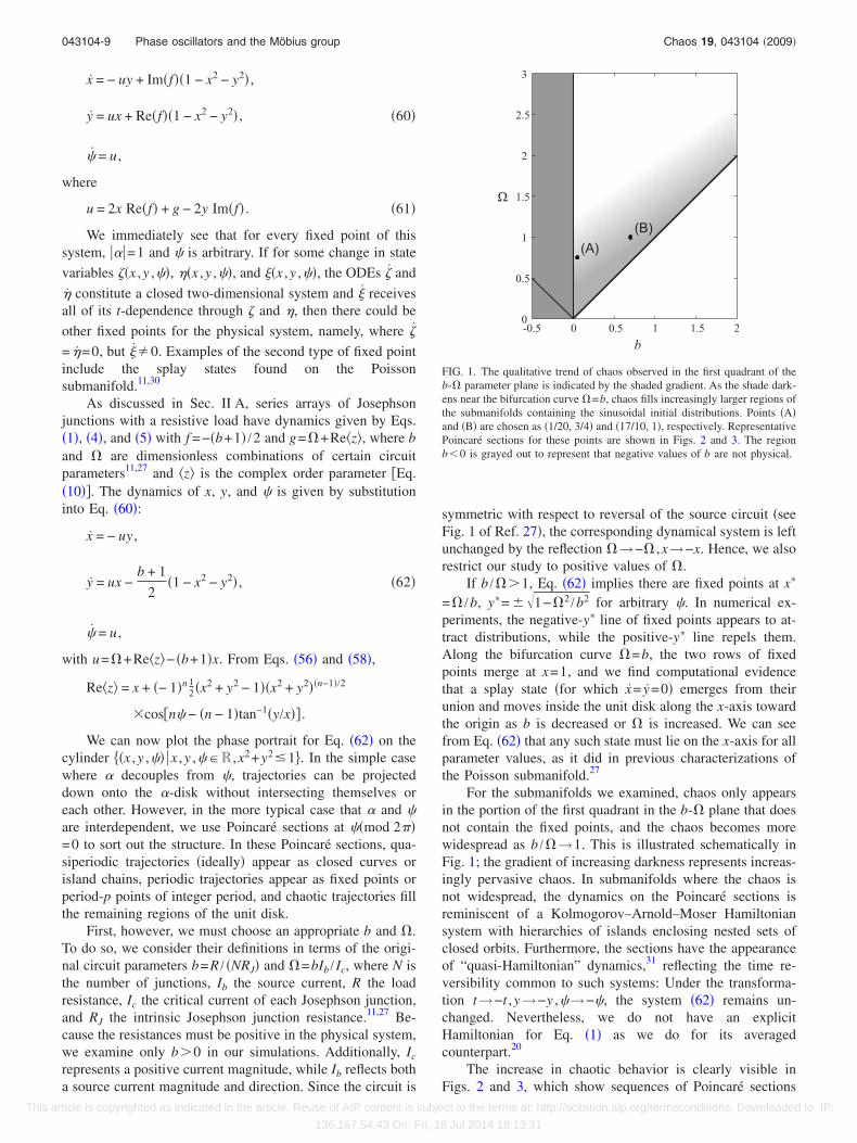
For the submanifolds we examined, chaos only appearsin the portion of the first quadrant in the b-� plane that doesnot contain the fixed points, and the chaos becomes morewidespread as b /�→1. This is illustrated schematically inFig. 1; the gradient of increasing darkness represents increas-ingly pervasive chaos. In submanifolds where the chaos isnot widespread, the dynamics on the Poincaré sections isreminiscent of a Kolmogorov–Arnold–Moser Hamiltoniansystem with hierarchies of islands enclosing nested sets ofclosed orbits. Furthermore, the sections have the appearanceof “quasi-Hamiltonian” dynamics,31 reflecting the time re-versibility common to such systems: Under the transforma-tion t→−t ,y→−y ,�→−�, the system �62� remains un-changed. Nevertheless, we do not have an explicitHamiltonian for Eq. �1� as we do for its averagedcounterpart.20

The increase in chaotic behavior is clearly visible inFigs. 2 and 3, which show sequences of Poincaré sections

Ω

b

(A)

(B)

-0.5 0 0.5 1 1.5 20

0.5

1

1.5

2

2.5

3

FIG. 1. The qualitative trend of chaos observed in the first quadrant of theb-� parameter plane is indicated by the shaded gradient. As the shade dark-ens near the bifurcation curve �=b, chaos fills increasingly larger regions ofthe submanifolds containing the sinusoidal initial distributions. Points �A�and �B� are chosen as �1/20, 3/4� and �17/10, 1�, respectively. RepresentativePoincaré sections for these points are shown in Figs. 2 and 3. The regionb 0 is grayed out to represent that negative values of b are not physical.

043104-9 Phase oscillators and the Möbius group Chaos 19, 043104 �2009�

This article is copyrighted as indicated in the article. Reuse of AIP content is subject to the terms at: http://scitation.aip.org/termsconditions. Downloaded to IP:

136.167.54.43 On: Fri, 18 Jul 2014 18:13:31

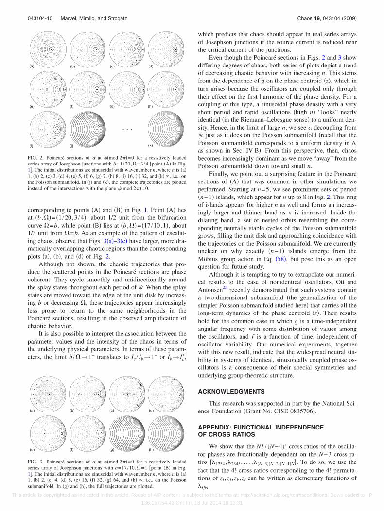
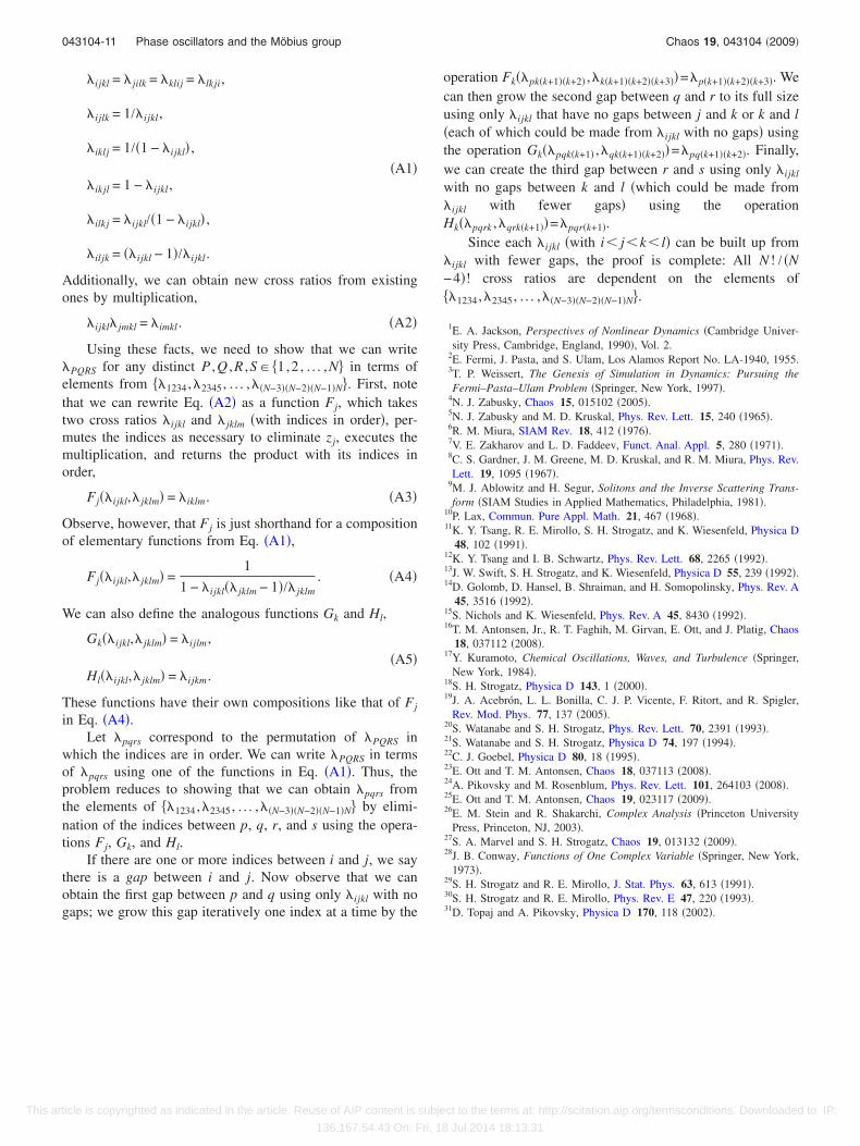
corresponding to points �A� and �B� in Fig. 1. Point �A� liesat �b ,��= �1 /20,3 /4�, about 1/2 unit from the bifurcationcurve �=b, while point �B� lies at �b ,��= �17 /10,1�, about1/3 unit from �=b. As an example of the pattern of escalat-ing chaos, observe that Figs. 3�a�–3�c� have larger, more dra-matically overlapping chaotic regions than the correspondingplots �a�, �b�, and �d� of Fig. 2.

Although not shown, the chaotic trajectories that pro-duce the scattered points in the Poincaré sections are phasecoherent: They cycle smoothly and unidirectionally aroundthe splay states throughout each period of �. When the splaystates are moved toward the edge of the unit disk by increas-ing b or decreasing �, these trajectories appear increasinglyless prone to return to the same neighborhoods in thePoincaré sections, resulting in the observed amplification ofchaotic behavior.

It is also possible to interpret the association between theparameter values and the intensity of the chaos in terms ofthe underlying physical parameters. In terms of these param-eters, the limit b /�→1− translates to Ic / Ib→1− or Ib→ Ic

+,

which predicts that chaos should appear in real series arraysof Josephson junctions if the source current is reduced nearthe critical current of the junctions.

Even though the Poincaré sections in Figs. 2 and 3 showdiffering degrees of chaos, both series of plots depict a trendof decreasing chaotic behavior with increasing n. This stemsfrom the dependence of g on the phase centroid �z�, which inturn arises because the oscillators are coupled only throughtheir effect on the first harmonic of the phase density. For acoupling of this type, a sinusoidal phase density with a veryshort period and rapid oscillations �high n� “looks” nearlyidentical �in the Riemann–Lebesgue sense� to a uniform den-sity. Hence, in the limit of large n, we see � decoupling from�, just as it does on the Poisson submanifold �recall that thePoisson submanifold corresponds to a uniform density in �,as shown in Sec. IV B�. From this perspective, then, chaosbecomes increasingly dominant as we move “away” from thePoisson submanifold down toward small n.

Finally, we point out a surprising feature in the Poincarésections of �A� that was common in other simulations weperformed. Starting at n=5, we see prominent sets of period�n−1� islands, which appear for n up to 8 in Fig. 2. This ringof islands appears for higher n as well and forms an increas-ingly larger and thinner band as n is increased. Inside thedilating band, a set of nested orbits resembling the corre-sponding neutrally stable cycles of the Poisson submanifoldgrows, filling the unit disk and approaching coincidence withthe trajectories on the Poisson submanifold. We are currentlyunclear on why exactly �n−1� islands emerge from theMöbius group action in Eq. �58�, but pose this as an openquestion for future study.

Although it is tempting to try to extrapolate our numeri-cal results to the case of nonidentical oscillators, Ott andAntonsen25 recently demonstrated that such systems containa two-dimensional submanifold �the generalization of thesimpler Poisson submanifold studied here� that carries all thelong-term dynamics of the phase centroid �z�. Their resultshold for the common case in which g is a time-independentangular frequency with some distribution of values amongthe oscillators, and f is a function of time, independent ofoscillator variability. Our numerical experiments, togetherwith this new result, indicate that the widespread neutral sta-bility in systems of identical, sinusoidally coupled phase os-cillators is a consequence of their special symmetries andunderlying group-theoretic structure.

ACKNOWLEDGMENTS

This research was supported in part by the National Sci-ence Foundation �Grant No. CISE-0835706�.

APPENDIX: FUNCTIONAL INDEPENDENCEOF CROSS RATIOS

We show that the N ! / �N−4�! cross ratios of the oscilla-tor phases are functionally dependent on the N−3 cross ra-tios ��1234,�2345, . . . ,��N−3��N−2��N−1�N�. To do so, we use thefact that the 4! cross ratios corresponding to the 4! permuta-tions of zi ,zj ,zk ,zl can be written as elementary functions of�ijkl,

(a) (b) (d)(c)

(e) (f) (h)(g)

(i) (j) (k)

. . .

FIG. 2. Poincaré sections of � at ��mod 2��=0 for a resistively loadedseries array of Josephson junctions with b=1 /20,�=3 /4 �point �A� in Fig.1�. The initial distributions are sinusoidal with wavenumber n, where n is �a�1, �b� 2, �c� 3, �d� 4, �e� 5, �f� 6, �g� 7, �h� 8, �i� 16, �j� 32, and �k� , i.e., onthe Poisson submanifold. In �j� and �k�, the complete trajectories are plottedinstead of the intersections with the plane ��mod 2��=0.

(a) (b) (d)(c)

(e) (f) (h)(g)

FIG. 3. Poincaré sections of � at ��mod 2��=0 for a resistively loadedseries array of Josephson junctions with b=17 /10,�=1 �point �B� in Fig.1�. The initial distributions are sinusoidal with wavenumber n, where n is �a�1, �b� 2, �c� 4, �d� 8, �e� 16, �f� 32, �g� 64, and �h� , i.e., on the Poissonsubmanifold. In �g� and �h�, the full trajectories are plotted.

043104-10 Marvel, Mirollo, and Strogatz Chaos 19, 043104 �2009�

This article is copyrighted as indicated in the article. Reuse of AIP content is subject to the terms at: http://scitation.aip.org/termsconditions. Downloaded to IP:

136.167.54.43 On: Fri, 18 Jul 2014 18:13:31

�ijkl = � jilk = �klij = �lkji,

�ijlk = 1/�ijkl,

�iklj = 1/�1 − �ijkl� ,

�A1��ikjl = 1 − �ijkl,

�ilkj = �ijkl/�1 − �ijkl� ,

�iljk = ��ijkl − 1�/�ijkl.

Additionally, we can obtain new cross ratios from existingones by multiplication,

�ijkl� jmkl = �imkl. �A2�

Using these facts, we need to show that we can write�PQRS for any distinct P ,Q ,R ,S� �1,2 , . . . ,N� in terms ofelements from ��1234,�2345, . . . ,��N−3��N−2��N−1�N�. First, notethat we can rewrite Eq. �A2� as a function Fj, which takestwo cross ratios �ijkl and � jklm �with indices in order�, per-mutes the indices as necessary to eliminate zj, executes themultiplication, and returns the product with its indices inorder,

Fj��ijkl,� jklm� = �iklm. �A3�

Observe, however, that Fj is just shorthand for a compositionof elementary functions from Eq. �A1�,

Fj��ijkl,� jklm� =1

1 − �ijkl�� jklm − 1�/� jklm. �A4�

We can also define the analogous functions Gk and Hl,

Gk��ijkl,� jklm� = �ijlm,

�A5�Hl��ijkl,� jklm� = �ijkm.

These functions have their own compositions like that of Fj

in Eq. �A4�.Let �pqrs correspond to the permutation of �PQRS in

which the indices are in order. We can write �PQRS in termsof �pqrs using one of the functions in Eq. �A1�. Thus, theproblem reduces to showing that we can obtain �pqrs fromthe elements of ��1234,�2345, . . . ,��N−3��N−2��N−1�N� by elimi-nation of the indices between p, q, r, and s using the opera-tions Fj, Gk, and Hl.

If there are one or more indices between i and j, we saythere is a gap between i and j. Now observe that we canobtain the first gap between p and q using only �ijkl with nogaps; we grow this gap iteratively one index at a time by the

operation Fk��pk�k+1��k+2� ,�k�k+1��k+2��k+3��=�p�k+1��k+2��k+3�. Wecan then grow the second gap between q and r to its full sizeusing only �ijkl that have no gaps between j and k or k and l�each of which could be made from �ijkl with no gaps� usingthe operation Gk��pqk�k+1� ,�qk�k+1��k+2��=�pq�k+1��k+2�. Finally,we can create the third gap between r and s using only �ijkl

with no gaps between k and l �which could be made from�ijkl with fewer gaps� using the operationHk��pqrk ,�qrk�k+1��=�pqr�k+1�.

Since each �ijkl �with i j k l� can be built up from�ijkl with fewer gaps, the proof is complete: All N ! / �N−4�! cross ratios are dependent on the elements of��1234,�2345, . . . ,��N−3��N−2��N−1�N�.

1E. A. Jackson, Perspectives of Nonlinear Dynamics �Cambridge Univer-sity Press, Cambridge, England, 1990�, Vol. 2.

2E. Fermi, J. Pasta, and S. Ulam, Los Alamos Report No. LA-1940, 1955.3T. P. Weissert, The Genesis of Simulation in Dynamics: Pursuing theFermi–Pasta–Ulam Problem �Springer, New York, 1997�.

4N. J. Zabusky, Chaos 15, 015102 �2005�.5N. J. Zabusky and M. D. Kruskal, Phys. Rev. Lett. 15, 240 �1965�.6R. M. Miura, SIAM Rev. 18, 412 �1976�.7V. E. Zakharov and L. D. Faddeev, Funct. Anal. Appl. 5, 280 �1971�.8C. S. Gardner, J. M. Greene, M. D. Kruskal, and R. M. Miura, Phys. Rev.Lett. 19, 1095 �1967�.

9M. J. Ablowitz and H. Segur, Solitons and the Inverse Scattering Trans-form �SIAM Studies in Applied Mathematics, Philadelphia, 1981�.

10P. Lax, Commun. Pure Appl. Math. 21, 467 �1968�.11K. Y. Tsang, R. E. Mirollo, S. H. Strogatz, and K. Wiesenfeld, Physica D

48, 102 �1991�.12K. Y. Tsang and I. B. Schwartz, Phys. Rev. Lett. 68, 2265 �1992�.13J. W. Swift, S. H. Strogatz, and K. Wiesenfeld, Physica D 55, 239 �1992�.14D. Golomb, D. Hansel, B. Shraiman, and H. Somopolinsky, Phys. Rev. A

45, 3516 �1992�.15S. Nichols and K. Wiesenfeld, Phys. Rev. A 45, 8430 �1992�.16T. M. Antonsen, Jr., R. T. Faghih, M. Girvan, E. Ott, and J. Platig, Chaos

18, 037112 �2008�.17Y. Kuramoto, Chemical Oscillations, Waves, and Turbulence �Springer,

New York, 1984�.18S. H. Strogatz, Physica D 143, 1 �2000�.19J. A. Acebrón, L. L. Bonilla, C. J. P. Vicente, F. Ritort, and R. Spigler,

Rev. Mod. Phys. 77, 137 �2005�.20S. Watanabe and S. H. Strogatz, Phys. Rev. Lett. 70, 2391 �1993�.21S. Watanabe and S. H. Strogatz, Physica D 74, 197 �1994�.22C. J. Goebel, Physica D 80, 18 �1995�.23E. Ott and T. M. Antonsen, Chaos 18, 037113 �2008�.24A. Pikovsky and M. Rosenblum, Phys. Rev. Lett. 101, 264103 �2008�.25E. Ott and T. M. Antonsen, Chaos 19, 023117 �2009�.26E. M. Stein and R. Shakarchi, Complex Analysis �Princeton University

Press, Princeton, NJ, 2003�.27S. A. Marvel and S. H. Strogatz, Chaos 19, 013132 �2009�.28J. B. Conway, Functions of One Complex Variable �Springer, New York,

1973�.29S. H. Strogatz and R. E. Mirollo, J. Stat. Phys. 63, 613 �1991�.30S. H. Strogatz and R. E. Mirollo, Phys. Rev. E 47, 220 �1993�.31D. Topaj and A. Pikovsky, Physica D 170, 118 �2002�.

043104-11 Phase oscillators and the Möbius group Chaos 19, 043104 �2009�

This article is copyrighted as indicated in the article. Reuse of AIP content is subject to the terms at: http://scitation.aip.org/termsconditions. Downloaded to IP:

136.167.54.43 On: Fri, 18 Jul 2014 18:13:31