iahr porto 2014 - paper template

E-proceedings of the 36th IAHR World Congress 28 June – 3 July, 2015, The Hague, the Netherlands

1

EVALUATION OF DESIGN HYDROGRAPH METHODS AND PROBABILISTIC METHODS FOR

ESTIMATING DESIGN WATER LEVELS ON THE RIVER MEUSE

J.C. POL(1)

, M. KOK(2)

, H.J. BARNEVELD(3)

, O. MORALES-NAPOLES(4)

& R.M.J. SCHIELEN(5)

(1) HKV Consultants, Lelystad, The Netherlands, [email protected]

(2) Delft University of Technology, Delft, The Netherlands, [email protected]

(3) HKV Consultants, Lelystad, The Netherlands, [email protected]

(4) Delft University of Technology, Delft, The Netherlands, [email protected],

(5) Ministry of Infrastructure and the Environment, Lelystad, The Netherlands, [email protected]

ABSTRACT

Design water levels are needed for the design of flood defences along the Dutch river Meuse. Current practise is that these water levels are determined by hydrodynamic simulation of a standard design hydrograph at the upstream gauging station Borgharen. The peak discharge of this synthetic hydrograph is based on a frequency analysis of the 100-year discharge dataset and its shape is determined by scaling and averaging all hydrographs in the dataset. Subsequently it is assumed that the simulated water levels along the river have the same return period as the peak discharge at Borgharen. This paper evaluates the accuracy of the current method and alternative methods to determine design water levels, using a dataset of 50,000 years of generated discharges at the station Borgharen based on extrapolation of rainfall events. The alternative methods include both design hydrograph methods and new methods that incorporate the hydrograph shape in a probabilistic way. The peak curvature is used as second stochastic variable in the probabilistic methods. The methods are evaluated by comparison with a reference set composed of 1D hydrodynamic simulations of all floods in the 50,000 year dataset. The results show that the currently used standard hydrograph method overestimates the design water levels up to 35 cm with respect to the reference. Alternative methods yield more accurate design water level estimates. The results obtained show no significant difference in accuracy between the probabilistic methods and the vertically averaged design hydrograph method.

Keywords: design water levels, hydrograph shape, probabilistic, Meuse, GRADE

1. INTRODUCTION

Design water levels and the equivalent water level frequency curves are basic concepts in flood risk management practice, both in The Netherlands and around the world. Water level frequency curves describe the relation between the magnitude and the likelihood of maximum water levels at a certain location. The design water level is the point on the frequency curve with a specified return period or exceedance frequency. These design water levels are used for the design of dikes and other flood protection measures, either in a deterministic design (e.g. TAW, 1998) or in a probabilistic assessment of the dike’s failure probability (Apel et al., 2004; Vrijling, 2001). Generally, water level records at the location of the flood defense are absent or too short to derive the design water level directly using a statistical/frequency analysis. Therefore data from a gauging station with a sufficiently long record is needed. In the case of the Dutch part of the river Meuse the upstream gauging station Borgharen is used (see Figure 1).

Different methods are available to transform the water levels at Borgharen into an design water level at a downstream location of interest. Two types of methods are distinguished; design hydrograph methods that use an (average) deterministic shape, and probabilistic methods that include the probability distributions of the hydrograph shape. This paper presents a comparison of these methods. Details of the methods are explained in chapter 3 and 4.

The Meuse basin is used as case study for this research. It has a length of 900 km and a catchment area of 33,000 km2.

Discharges vary from 10 m3/s in summer to 3000 m

3/s in winter, and respond strongly to rainfall. The combination of a

dynamic rain-fed character and large variations in bed profile, such as large storage areas in the Dutch part of the river, leads to a river system in which wave damping is important. Wave damping is strongly influenced by the hydrograph shape. Figure 1 shows an overview of the catchment and relevant locations. Results are presented for location Mook, which is located along the river reach where the hydrograph shape has relatively much influence.

1.1 Approaches to incorporate hydrograph shape in design water levels

The current Dutch approach (Ministerie van V&W, 2007) to determine these design water levels is to derive a design hydrograph at Borgharen, and simulate this design flood using 2D hydrodynamic models to derive the corresponding design water level at the location of interest. Design hydrographs have a peak discharge with exceedance frequency 1/T which is found by frequency analysis (Hamed & Rao, 2000), and a shape which is found by for example averaging all hydrograph shapes in the dataset. The standard averaging method that is currently used for the Dutch Meuse was

mailto:[email protected]

mailto:[email protected]

E-proceedings of the 36th IAHR World Congress, 28 June – 3 July, 2015, The Hague, the Netherlands

2

developed by Klopstra & Vrisou van Eck (1999) and adapted by Wijbenga & Stijnen (2004). An alternative – the vertical averaging method – was proposed recently by Ogink (2012). Despite its application for years, no study is known that compares the design water levels derived by the standard method to a sufficiently large reference set of known local water levels.

Design hydrograph methods in general have two potential limitations. First, this design hydrograph approach focuses on the peak discharge as primary stochastic variable. It is known that the hydrograph shape is also an important stochastic variable which affects the downstream design water levels through peak attenuation effects (Gerretsen, 2009; Woltemade & Potter, 1994). Closely related to this first remark is a crucial but seldom mentioned assumption in the design hydrograph methods, namely that a 1/T peak discharge at the gauging station leads to a 1/T water level at all locations along the river, provided that this average hydrograph shape is used. This assumption has not been confirmed yet. This paper shows to what extent this assumption is valid in the case of the river Meuse.

Probabilistic methods include the probability of occurrence of hydrograph shapes in the analysis, and couple this probability with the effects that different hydrograph shapes have on water levels. This paper describes and analyses two probabilistic methods: an explicit and an implicit method. The explicit method is based on the work of Geerse (2013), in which the water level frequency curve is expressed as function of the probability distributions of peak discharge and shape. The implicit method is a simplification of the explicit method, and uses no distribution functions.

Figure 1. The Meuse river basin (De Wit, 2008) and relevant locations in The Netherlands.

Chapter 2 gives a short overview of the approach, after which both a description and intermediate results of the different methods are given in Chapters 3 (design hydrograph methods) and Chapter 4 (probabilistic methods). Chapter 5 gives the main results: a comparison of water level frequency curves for each method. The paper ends with discussion and conclusions in Chapters 6 and 7.

2. RESEARCH APPROACH

As is indicated in the introduction, this paper considers different methods to incorporate the effect of hydrograph shape in the computation of design water levels or water level exceedance frequencies:

Standard hydrograph method;

Standard hydrograph method with modified selection interval;

Vertically averaged hydrograph method;

Vertically averaged hydrograph method with modified selection interval;

Explicit probabilistic method;

Implicit probabilistic method;

Simulation of complete dataset (reference set). All methods were applied to the same dataset and the same hydraulic model such that we can make a clear comparison between the methods.

2.1 Discharge dataset

One of the reasons why the probabilistic methods are not widely applied, is a lack of data. Although the discharge records at Borgharen cover more than 100 years, this set is rather small for evaluating design water levels with return periods of 1,000 to 10,000 years, being actual protection levels in The Netherlands. Probabilistic analyses of both peak discharge and hydrograph shape require even more data.

E-proceedings of the 36th IAHR World Congress

28 June – 3 July, 2015, The Hague, the Netherlands

3

Instead of the 100-year measured dataset, this research used a 50,000 year simulated discharge dataset from the GRADE (Generator of Rainfall And Discharge Extremes) project (De Wit and Buishand, 2007). Rainfall resampling techniques and a hydrological model of the Meuse basin have been combined to generate these discharge series. Details on derivation and validation of this dataset are given in Leander et al. (2005) and Kramer & Schroevers (2008). This GRADE discharge dataset provides a large collection of flood waves with a realistic variation in peak discharge and shape. Due to its size, the GRADE dataset allows to establish a reference set with hydrodynamic simulation of all floods in this dataset and allows to evaluate the accuracy of the different methods.

From the 50,000 years of daily discharge data, flood events were selected with a peak discharge (Qp) larger than 1750 m

3/s and no higher peak present in a period of 10 days before and after the peak. As a result of this 10 day interval, two

peaks close to each other are defined as one flood event. Selection according to this definition yields 17,232 flood events from this 50,000 year data set. A flood hydrograph is defined by the discharge in the period between 15 days before the flood peak and 15 days after the flood peak.

2.2 Hydrodynamic model

A hydrodynamic model is applied in all methods to determine the downstream water levels for a given inflow hydrograph. Because of the large number of simulations involved in the reference set (see paragraph 4.5), we used a relatively fast 1D SOBEK model of the Dutch part of the Meuse, which reflects the state of the river system in the year 2014. This model is currently used for in the flood early warning system for the Dutch part of the Meuse River. In the model simulations the model characteristics were kept the same, except the inflow hydrograph and tributary inflows. Tributary flows are determined through statistical relations between the measured tributary flow and measured discharge in the Meuse River (Van der Veen, 2005).

3. DESIGN HYDROGRAPH METHODS

3.1 Method

The peak discharge with return period T is found by flood frequency analysis (e.g. Hamed & Rao, 2000). We have chosen for a peaks over threshold (POT) approach with a threshold of 1750 m

3/s (T ≈ 3 year) and a Weibull plotting position. then

the return period for an event is given by:

1 1( )

e e

R N RT i

p N i N

[1]

where p is the Weibull plotting position (i/N+1), i is the rank of the flood event (i=1 is largest, i=Ne is smallest), Ne is the total number of flood events, and R the length of the discharge record (years).

In both evaluated design hydrograph methods, the shape of the design hydrograph is found by averaging all hydrograph shapes in the GRADE dataset. The first step is to scale all hydrographs to a peak discharge equal to the design discharge (Qp,d); i.e. multiply all discharge values with Qp,d/Qp (Figure 2, left). Subsequently, in the standard method, the total duration (rising and falling duration) is determined for each hydrograph at a number of discharge levels. The average duration per level is given by the median of the durations at this discharge level, assuming a lognormal distribution. The standard hydrograph shape is constructed by connection these points at all discharge levels. In the vertical averaging method the discharges of the scaled hydrographs are averaged at a number of time steps, instead of the durations at a number of discharge levels (Figure 2, left). Vertical averaging leads generally to a narrower design hydrograph, and thus to lower water levels downstream. These standard and vertically averaged design hydrograph shapes were applied to seven design peak discharges of 2600, 3280, 3800, 4000, 4200, 4400 and 4600 m

3/s. The resulting design water levels

are shown in Figure 8.

Figure 2. Standard and vertical averaging method (left) and influence of selection interval (right)


4

3.2 Modification of the flood selection interval

In the standard hydrograph method (described above), the same hydrograph shape is applied to different design peak discharges. However, hydrographs in the extreme range have a different shape than ones from more moderate floods (Figure 2), for instance because coincidence of tributary peaks leads to high and narrow hydrographs and a lag-time between tributaries leads to lower and wider hydrographs. To show how the standard hydrograph shape depends on the flood magnitude, standard shapes were also derived by averaging only floods from specific discharge classes. For example the shape of the Qp=3800 m

3/s standard hydrograph is found by averaging the floods with 3500<Qp<4000. This

modification of the design hydrograph procedure is indicated by ‘modified selection interval’.

4. PROBABILISTIC METHODS

Design hydrograph methods treat the peak discharge in a probabilistic way, but use a deterministic (average) shape. In contrast with design hydrograph methods, probabilistic methods incorporate the influence of shape by taking into account the effects of different shapes on local water levels and the probability that these shapes occur. Paragraph 4.1 identifies the shape variables that affect water levels, and which are used in the transformation function (paragraph 4.2) that is used by both probabilistic methods.

4.1 Influence of hydrograph shape variables

In order to choose one or more variables to represent the influence of shape, it was investigated which variables at Borgharen can predict the downstream water levels most accurately. Variables that are considered are the peak discharge (Qp), flood volume above level L (VL), flood duration at level L (DL) and peak curvature (C2). Four threshold levels L were applied: 0 m

3/s and 1250 m

3/s (bankfull discharge) and 50% and 85% of the peak discharge (see Figure 3).

The peak curvature is an approximation of the second derivative of the discharge around the peak, divided by Qp and multiplied by 10

12:

212 12

2 2

( ) ( ) 2 110 10

p p p

p p

Q t dt Q t dt Q QC

Q dt t Q

[2]

where dt = 2*24*3600 s (two days before and after the peak)

V85%

Q=0.85∙Qp

Q(tp+dt) Q(tp-dt)

Q=0.5∙Qp

Q=1250

Qp

Figure 3. Definition of hydrograph shape variables

Which variables Xi should be used in the analyses was decided with the use of a correlation1 analysis. The first variable

Xa is selected by the highest Spearman rank correlation coefficient ρs(Xi,Y). The second variable Xb is selected by the highest mean conditional rank correlation coefficient ρs(Xi,Y|Xa). Since the value of ρs(Xi,Y|Xa) generally varies for different values of Xa , the mean is used to select the second variable. The reason why the conditional correlation was used for the second variable, is that the second highest Spearman rank correlation coefficient does not indicate the additional predictive power of a variable. When two variables are fully correlated, both can have a high Spearman coefficient, but the second does not add any information to the first. In this research, two variables were used. For analyses with more than two variables, this procedure can be easily extended.

1 Since the hydrograph variables are given upstream of the local water levels, it is reasonable to assume that the water levels are not

only correlated to but also caused by the hydrograph variables.



5

Table 1 shows the Spearman rank correlation between water levels and shape variables. Not very surprisingly, the Qp has generally the strongest correlation with hmax,x, together with V1250 (volume above the bankfull discharge). Since Qp and V1250 are strongly correlated (ρs = 0.85), one could use either variable. The peak discharge Qp was chosen for further analysis because it is widely used as most important predictor of water levels.

Table 1. Spearman rank correlation between variables (columns) and water levels at five locations (rows)

QP D1250 D50% D85% V0 V1250 V50% V85% C2

MAASEIK 0.993 0.562 -0.085 0.016 0.660 0.887 0.405 0.538 -0.061

VENLO 0.963 0.644 0.009 0.152 0.729 0.934 0.512 0.654 -0.197

MOOK 0.933 0.695 0.072 0.238 0.768 0.957 0.580 0.720 -0.272

MEGEN 0.927 0.704 0.084 0.252 0.774 0.960 0.593 0.731 -0.285

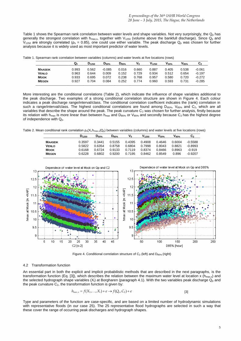
More interesting are the conditional correlations (Table 2), which indicate the influence of shape variables additional to the peak discharge. Two examples of a strong conditional correlation structure are shown in Figure 4. Each colour indicates a peak discharge range/interval/class. The conditional correlation coefficient indicates the (rank) correlation in such a range/interval/class. The highest conditional correlations are found among D85%, V85% and C2, which are all variables that describe the shape around the peak. The peak curvature C2 was chosen for further analysis, firstly because its relation with hmax is more linear than between hmax and D85% or V85% and secondly because C2 has the highest degree of independence with Qp.

Table 2. Mean conditional rank correlation ρs(Xi,hmax,x|Qp) between variables (columns) and water levels at five locations (rows)

D1250 D50% D85% V0 V1250 V50% V85% C2

MAASEIK 0.3597 0.3441 0.5155 0.4395 0.4908 0.4646 0.6004 -0.5588

VENLO 0.5822 0.6354 0.8758 0.6804 0.7998 0.8043 0.8821 -0.8993

MOOK 0.6168 0.6724 0.9133 0.7119 0.8374 0.8466 0.8963 -0.919

MEGEN 0.6228 0.6802 0.9200 0.7195 0.8462 0.8549 0.896 -0.9207

Figure 4. Conditional correlation structure of C2 (left) and D85% (right)

4.2 Transformation function

An essential part in both the explicit and implicit probabilistic methods that are described in the next paragraphs, is the transformation function (Eq. [3]), which describes the relation between the maximum water level at location x (hmax,x) and the selected hydrograph shape variables (Xi) at Borgharen (paragraph 4.1). With the two variables peak discharge Qp and the peak curvature C2, the transformation function is given by:

, 1 2( , , ) ( , )max x i ph f X X f Q C [3]

Type and parameters of the function are case-specific, and are based on a limited number of hydrodynamic simulations with representative floods (in our case 25). The 25 representative flood hydrographs are selected in such a way that these cover the range of occurring peak discharges and hydrograph shapes.


6

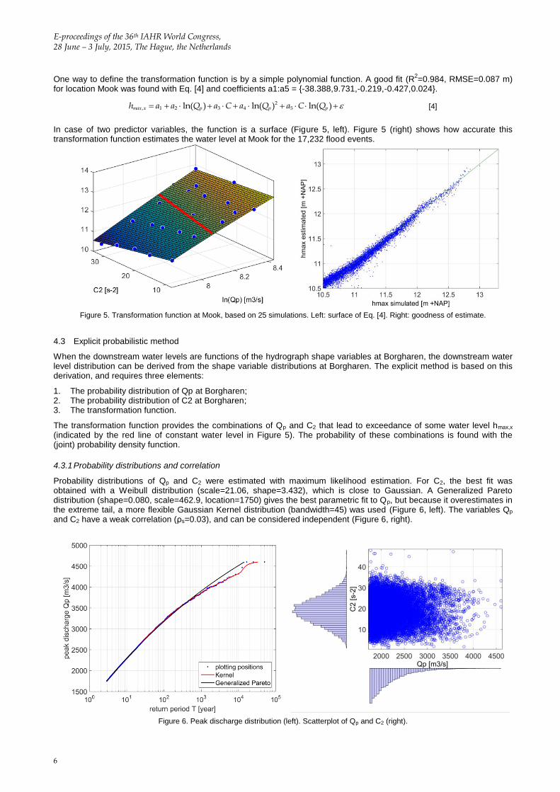
One way to define the transformation function is by a simple polynomial function. A good fit (R2=0.984, RMSE=0.087 m)

for location Mook was found with Eq. [4] and coefficients a1:a5 = {-38.388, 9.731, -0.219, -0.427, 0.024}.

2, 1 2 3 4 5ln( ) ln( ) ln( )max x p p ph a a Q a C a Q a C Q [4]

In case of two predictor variables, the function is a surface (Figure 5, left). Figure 5 (right) shows how accurate this transformation function estimates the water level at Mook for the 17,232 flood events.

Figure 5. Transformation function at Mook, based on 25 simulations. Left: surface of Eq. [4]. Right: goodness of estimate.

4.3 Explicit probabilistic method

When the downstream water levels are functions of the hydrograph shape variables at Borgharen, the downstream water level distribution can be derived from the shape variable distributions at Borgharen. The explicit method is based on this derivation, and requires three elements:

1. The probability distribution of Qp at Borgharen; 2. The probability distribution of C2 at Borgharen; 3. The transformation function.

The transformation function provides the combinations of Qp and C2 that lead to exceedance of some water level hmax,x (indicated by the red line of constant water level in Figure 5). The probability of these combinations is found with the (joint) probability density function.

4.3.1 Probability distributions and correlation

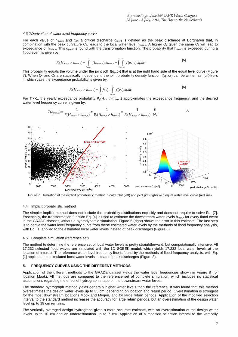
Probability distributions of Qp and C2 were estimated with maximum likelihood estimation. For C2, the best fit was obtained with a Weibull distribution (scale=21.06, shape=3.432), which is close to Gaussian. A Generalized Pareto distribution (shape=0.080, scale=462.9, location=1750) gives the best parametric fit to Qp, but because it overestimates in the extreme tail, a more flexible Gaussian Kernel distribution (bandwidth=45) was used (Figure 6, left). The variables Qp and C2 have a weak correlation (ρs=0.03), and can be considered independent (Figure 6, right).

Figure 6. Peak discharge distribution (left). Scatterplot of Qp and C2 (right).



7

4.3.2 Derivation of water level frequency curve

For each value of hmax,x and C2, a critical discharge qp,crit is defined as the peak discharge at Borgharen that, in combination with the peak curvature C2, leads to the local water level hmax,x. A higher Qp given the same C2 will lead to exceedance of hmax,x. This qp,crit is found with the transformation function. The probability that hmax,x is exceeded during a flood event is given by:

max, ,

max, max, max, max,( ) ( ) ( , )x p crit

e x x x x p p

h q

P H h f h dh f q c dq dc

[5]

This probability equals the volume under the joint pdf f(qp,c2) that is at the right hand side of the equal level curve (Figure 7). When Qp and C2 are statistically independent, the joint probability density function f(qp,c2) can be written as f(qp)∙f(c2), in which case the exceedance probability is given by:

,

max, max,( ) ( ) ( )p crit

e x x p p

q

P H h f c f q dq dc

[6]

For T>>1, the yearly exceedance probability Py(Hmax,x>hmax,x) approximates the exceedance frequency, and the desired water level frequency curve is given by:

max,

max, max, max, max, max, max,

1 1 1( )

( ) ( ) ( )x

x x y x x e x x e

RT h

F H h P H h P H h N

[7]

Figure 7. Illustration of the explicit probabilistic method. Scatterplot (left) and joint pdf (right) with equal water level curve (red line).

4.4 Implicit probabilistic method

The simpler implicit method does not include the probability distributions explicitly and does not require to solve Eq. [7]. Essentially, the transformation function Eq. [4] is used to estimate the downstream water levels hmax,x for every flood event in the GRADE dataset, without a hydrodynamic simulation. Figure 5 (right) shows the error in this estimate. The last step is to derive the water level frequency curve from these estimated water levels by the methods of flood frequency analysis, with Eq. [1] applied to the estimated local water levels instead of peak discharges (Figure 8).

4.5 Complete simulation (reference set)

The method to determine the reference set of local water levels is pretty straightforward, but computationally intensive. All 17,232 selected flood waves are simulated with the 1D SOBEK model, which yields 17,232 local water levels at the location of interest. The reference water level frequency line is found by the methods of flood frequency analysis, with Eq. [1] applied to the simulated local water levels instead of peak discharges (Figure 8).

5. FREQUENCY CURVES USING THE DIFFERENT METHODS

Application of the different methods to the GRADE dataset yields the water level frequencies shown in Figure 8 (for location Mook). All methods are compared to the reference set of complete simulation, which includes no statistical assumptions regarding the effect of hydrograph shape on the downstream water levels.

The standard hydrograph method yields generally higher water levels than the reference. It was found that this method overestimates the design water levels up to 35 cm, depending on location and return period. Overestimation is strongest for the most downstream locations Mook and Megen, and for large return periods. Application of the modified selection interval to the standard method increases the accuracy for large return periods, but an overestimation of the design water level up to 19 cm remains.

The vertically averaged design hydrograph gives a more accurate estimate, with an overestimation of the design water levels up to 10 cm and an underestimation up to 7 cm. Application of a modified selection interval to the vertically


8

averaged hydrograph does not improve the accuracy significantly. Generally, the vertical averaging method tends to be slightly lower than the reference, whereas the standard method tends to be slightly higher.

The two probabilistic methods which have been applied give accurate estimates of the water level frequency curves, but do not improve the estimate of vertical averaging. The differences between implicit and the reference can be related directly to the error in the transformation function shown in Figure 5 (right). In the very extreme tail, the explicit method gives slightly higher water levels than implicit, which is expected to be the result of the goodness of fit of the joint probability distribution of Qp and C2.

Figure 8 shows some flattening of the reference frequency curve for 103<T<10

4, which is also found at locations further

downstream (Megen). An explanation for this behaviour is the large retention basin Lob van Gennep, just upstream of Mook. The retention basin limits the water levels, up to a certain level when the storage capacity is insufficient. In the design hydrograph methods this discontinuity is even more pronounced. At more upstream locations, where there is little flood wave damping and little influence of the hydrograph shape on water levels, the curve follows a more continuous line and the different methods yield approximately the same result.

Figure 8. Water level frequency curves and design water levels at Mook using the five methods

6. DISCUSSION

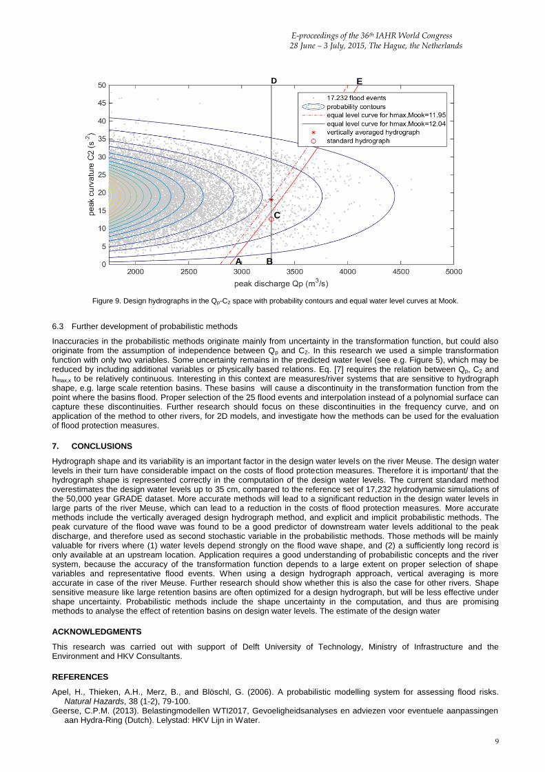
6.1 Validity of design hydrograph assumption

The validity of the central assumption in the design hydrograph approach – that a design hydrograph with 1/T peak discharge leads to a 1/T local water level – is clarified in Figure 9. Focussing on the standard hydrograph (Qp=3280 m

3/s,

C2=12.6*1012

s-2

, hmax,Mook=12.04 m +NAP), the assumption is only valid if the probability in the triangle ABC equals the probability in triangle CDE. In this case, CDE has a larger probability than ABC, which means that the exceedance frequency is overestimated (return period underestimated). The vertically averaged hydrograph has a position where the assumption is approximately valid, which is an explanation for the high accuracy of the vertical averaging method. This does not show that the vertical hydrograph is always better, since that depends on the inclination of the equal water level curve. When these equal water level curves change over the locations along the river, there cannot exist a single design hydrograph that represents the exceedance frequency correctly for all locations/situations. In rivers where the influence of shape is large or the shape distribution is asymmetric.

6.2 Comparison of methods

An important question is which (dis)advantages the different estimation methods could have for application in water management practice (in The Netherlands). Important considerations include accuracy, simplicity and computational effort. The probabilistic methods are generally more demanding, in complexity of the analysis or in computational effort. Complete simulation (reference) is the most accurate method, and relatively simple, but requires a lot of computational time, especially when 2D simulations are required. Of course the amount of simulations can be reduced by increasing the threshold of 1750 m

3/s when one is only interested in the more extreme water levels. The explicit and implicit methods

require only a limited number of simulations to characterize the influence of shape. The implicit method has the advantage that it is more simple than the explicit method, especially in case of dependent hydrograph shape variables. In those cases, the explicit method requires a multivariate distribution of different distribution types. Both the explicit and implicit methods are very suitable to study the effects of climate change, since hydrodynamic simulation results are not coupled to flood statistics at Borgharen, unlike in the design hydrograph approaches. The design hydrograph methods are relatively simple to apply once the design hydrograph is defined, but are less accurate. Amongst the design hydrograph methods, vertical averaging is most accurate.



9

Figure 9. Design hydrographs in the Qp-C2 space with probability contours and equal water level curves at Mook.

6.3 Further development of probabilistic methods

Inaccuracies in the probabilistic methods originate mainly from uncertainty in the transformation function, but could also originate from the assumption of independence between Qp and C2. In this research we used a simple transformation function with only two variables. Some uncertainty remains in the predicted water level (see e.g. Figure 5), which may be reduced by including additional variables or physically based relations. Eq. [7] requires the relation between Qp, C2 and hmax,x to be relatively continuous. Interesting in this context are measures/river systems that are sensitive to hydrograph shape, e.g. large scale retention basins. These basins will cause a discontinuity in the transformation function from the point where the basins flood. Proper selection of the 25 flood events and interpolation instead of a polynomial surface can capture these discontinuities. Further research should focus on these discontinuities in the frequency curve, and on application of the method to other rivers, for 2D models, and investigate how the methods can be used for the evaluation of flood protection measures.

7. CONCLUSIONS

Hydrograph shape and its variability is an important factor in the design water levels on the river Meuse. The design water levels in their turn have considerable impact on the costs of flood protection measures. Therefore it is important/ that the hydrograph shape is represented correctly in the computation of the design water levels. The current standard method overestimates the design water levels up to 35 cm, compared to the reference set of 17,232 hydrodynamic simulations of the 50,000 year GRADE dataset. More accurate methods will lead to a significant reduction in the design water levels in large parts of the river Meuse, which can lead to a reduction in the costs of flood protection measures. More accurate methods include the vertically averaged design hydrograph method, and explicit and implicit probabilistic methods. The peak curvature of the flood wave was found to be a good predictor of downstream water levels additional to the peak discharge, and therefore used as second stochastic variable in the probabilistic methods. Those methods will be mainly valuable for rivers where (1) water levels depend strongly on the flood wave shape, and (2) a sufficiently long record is only available at an upstream location. Application requires a good understanding of probabilistic concepts and the river system, because the accuracy of the transformation function depends to a large extent on proper selection of shape variables and representative flood events. When using a design hydrograph approach, vertical averaging is more accurate in case of the river Meuse. Further research should show whether this is also the case for other rivers. Shape sensitive measure like large retention basins are often optimized for a design hydrograph, but will be less effective under shape uncertainty. Probabilistic methods include the shape uncertainty in the computation, and thus are promising methods to analyse the effect of retention basins on design water levels. The estimate of the design water

ACKNOWLEDGMENTS

This research was carried out with support of Delft University of Technology, Ministry of Infrastructure and the Environment and HKV Consultants.

REFERENCES

Apel, H., Thieken, A.H., Merz, B., and Blöschl, G. (2006). A probabilistic modelling system for assessing flood risks. Natural Hazards, 38 (1-2), 79-100.

Geerse, C.P.M. (2013). Belastingmodellen WTI2017, Gevoeligheidsanalyses en adviezen voor eventuele aanpassingen aan Hydra-Ring (Dutch). Lelystad: HKV Lijn in Water.

E D

C

A B


10

Gerretsen, J.H. (2009). Flood level prediction for regulated rain-fed rivers (Ph.D. Thesis). Enschede: University of Twente.

Hamed, K., and Rao, A. (2000). Flood frequency analysis. Boca Raton: CRC press.

Klopstra, D., and Vrisou van Eck, N. (1999). Methodiek voor vaststelling van de vorm van de maatgevende afvoergolf van de Maas bij Borgharen (Dutch). Lelystad: HKV Lijn in Water.

Kramer, N. and Schroevers, R. (2008). Generator of Rainfall and Discharge Extremes (GRADE), part F. Delft: Deltares. Leander, R., Buishand, T.A., Aalders, P., and Wit, M.J.M. de (2005). Estimation of extreme floods of the river Meuse

using a stochastic weather generator and a rainfall–runoff model/Estimation des crues extrêmes de la Meuse à l'aide d'un générateur stochastique de variables météorologiques et d'un modèle pluie–débit. Hydrological Sciences Journal, 50 (6), 1089-1103.

Ministerie van V&W (2007). Hydraulische randvoorwaarden primaire waterkeringen voor de derde toetsronde 2006-2011 (HR 2006) (Dutch). The Hague: Ministerie van Verkeer en Waterstaat.

Ogink, H.J.M. (2012). Design discharge and design hydrograph computation for Meuse and Rhine rivers: comparison of computational methods. (unpublished document).

TAW (1998). Fundamentals on Water Defences. Delft: Technische Adviescommissie voor de Waterkeringen. Veen, R. van der (2005). Laterale toestroming Maas en Rijn onder maatgevende omstandigheden (Dutch). Arnhem:

Rijkswaterstaat - RIZA. Vrijling, J.K. (2001). Probabilistic design of water defense systems in The Netherlands. Reliability Engineering & System

Safety, 74 (3), 337-344. Wijbenga, J.H.A. and Stijnen, J. (2004). Aanpassingen golfvormgenerator (Dutch). Lelystad: HKV Lijn in Water. Wit, M.J.M. de (2008). Van regen tot Maas (Dutch). Diemen: Veen magazines. Wit, M.J.M. de, and Buishand, T.A. (2007). Generator of Rainfall And Discharge Extremes (GRADE) for the Rhine and

Meuse basins. Lelystad: Rijkswaterstaat and KNMI Woltemade, C.J., and Potter, K.W. (1994). A watershed modeling analysis of fluvial geomorphologic influences on flood

peak attenuation. Water Resources Research, 30 (6), 1933-1942.

iahr porto 2014 - paper template

Documents