hydraulics 1: course notes the pressure increases as z decreases (or depth increases). integrating...

G F Lane-Serff 1 18-Feb-09

Hydraulics 1: Course notes Staff Dr G F Lane-Serff Extn 64602, room P/B20, [email protected] Course Outline

Hydraulics I A Fluid properties

A1 Introduction: Fluids, continuum and density A2 Viscosity, surface tension and pressure A3 Tutorial: fluid properties

B Hydrostatics B1 Hydrostatic pressure and the hydrostatic equation B2 Pressure measurement B3 Hydrostatic force on a plane surface B4 Buoyancy and Archimedes Principle B5 Hydrostatic force on a curved surface B6 Tutorial: Hydrostatics

C Kinematics and continuity C1 Kinematics C2 Conservation of mass: continuity C3 Tutorial: Kinematics and continuity

D Energy and momentum: Principles D1 Conservation of energy: Bernoulli's Equation D2 Bernoulli's Equation: Applications to flow measurement D3 Momentum principle: control volumes D4 Momentum principle: open channel flow D5 Tutorial: forces and hydraulic jumps

E Pipeflow E1 Reynolds Experiment: Laminar and turbulent flow E2 Pipeflow: laminar flow E3 Flow from static reservoir (no energy losses) E4 Turbulent flow and head loss E5 Pipeflow: other head losses E6 Tutorial: Pipeflow

F Energy and momentum: further applications F1 Sharp expansions and orifice meters F2 Momentum principle: effects of gravity F3 Tutorial: Gravity and flow measurement

Assessment Coursework (laboratory work and problems):

Fluid properties and hydrostatics 5% Momentum and energy 5%

Pipeflow network design project 10% Exam: Four out of six questions (free choice) 80% Books Massey BS (revised Ward-Smith), Mechanics of Fluids. 532 Chadwick AJ and Morfett JC (and Borthwick M, for later editions), Hydraulics in Civil and Environmental Engineering. 627 Hamill L, Understanding Hydraulics. 627 White FM, Fluid Mechanics. 532 Douglas JF and Matthew RD, Solving Problems in Fluid Mechanics. 532 Featherstone RE and Nalluri, Civil Engineering Hydraulics. 627


Hydraulics I

A Fluid properties

A1 Introduction: Fluids, continuum and density Definition of a fluid A fluid is a substance that flows. A fluid deforms continuously under the influence of an applied force, whereas a solid deforms a finite amount and then resists further deformation. This is because a solid can sustain a static internal shear stress whereas a fluid cannot. The molecules of a fluid are not held in a fixed arrangement and can move past each other. Fluids include liquids and gases, and for civil engineers the most important fluids are water and air. As civil engineers, you need to understand the behaviour of fluids in both the built and natural environment. Engineers study flow in reservoirs, pipes, water and waste water treatment, and building ventilation, and also river flooding, groundwater flows, waves and wind loading on structures. Continuum Hypothesis Although a fluid is made up of individual molecules, at any scale significantly larger than the separation between molecules we can approximate the fluid as effectively continuous. This means we can regard properties such as temperature, pressure, density and velocity as functions of positions in space, and apply differential calculus to derive equations. There are applications where this approach is not valid: these include nanotechnology (operating at scales comparable to those of the fluid molecules) or in environments where the molecular separation becomes significant compared with the scale of motion we are interested in (e.g. aerospace applications at the edge of the atmosphere). Density Density is defined as mass per unit volume. It is usually denoted by the Greek letter ρ. In SI units density is given in kg m-3. In general the density can vary at different points in space and at different times so ρ(x,t), although we will generally deal with uniform fixed density. The typical density of (fresh) water is approximately ρwater = 1000 kg m-3, and changes relatively little at normal temperatures and pressures. However, we will also consider problems where we have seawater rather than fresh water. The salt in seawater increases the density, so that a typical seawater density is ρseawater ~ 1026 to 1028 kg m-3 (depending on the salt concentration), while water in estuaries will lie somewhere between the fresh water and seawater values. A typical air density is ρair ~1.2 kg m-3, but like all gases, the density of air varies more with pressure and temperature than the density of water. This is because gases are more easily compressed than liquids. We will discuss this in more detail later. Specific weight Whereas density is mass per unit volume, specific weight is weight per unit volume: γ = ρg. Relative density or specific gravity The relative density is the density relative to some standard or reference density. Generally only used for liquids rather than gases, and so the reference density is often the density of water. The relative density is sometimes referred to as the specific gravity (s.g.). Thus if a manometer fluid has a specific gravity of 0.75, then it has a density of 750 kg m-3. Note that relative density has no units (“dimensionless”).


A2 Viscosity, surface tension and pressure Viscosity As the fluid molecules move past each other there is a resistance to this relative motion. While the stress in a solid depends on the amount of deformation (strain) of the solid, for a fluid it is the rate of deformation (strain rate) that is related to the stress. The velocity profile in a fluid near a solid boundary typically has the form shown below: Fluid further from the boundary is moving faster, and the relative motion of one layer past another is resisted by intermolecular forces in the fluid. The resistance is in the form of a stress (a force per unit area), and is generally found to be linearly dependent on the strain rate (shear or velocity gradient). Thus the stress, τ, is given by

τ = µ dudz .

The constant of proportionality is known as the viscosity (or coefficient of viscosity or dynamic viscosity) and is usually denoted by µ. Stress has units of force/area: N m-2 or Pa, while shear has units of s-1. Thus the units of viscosity can be written as Pa s, or alternatively as kg m-1 s-1. Fluids for which there is a linear relation between stress and shear are known as Newtonian fluids, and include water and air. Typical values for viscosity are:

µair = 1.8×10-5 kg m-1 s-1, µwater = 10-3 kg m-1 s-1, while µglycerin = 1.5 kg m-1 s-1. However, viscosity depends strongly on temperature. The force acts to oppose the motion, so in the example above there is a force by the fluid on the boundary tending to move the boundary to the right (and an equal and opposite force on the fluid slowing it down). The fluid in contact with the boundary cannot move (u = 0) otherwise there would be an infinite viscous force. This is known as the no-slip condition. Example A square block (of side 0.3 m) moving at 2 m/s on a thin (2mm) layer of water. Assuming a linear velocity profile what is the force on block?

Shear = dudz = 2/0.002 = 1000 s-1

Stress

τ = µ dudz = 1000 × 10-3 = 1 N m-2

Force = τ × area = 1×0.3×0.3 = 0.09 N.

z

u(z)


Surface tension Any free surface (or interface between immiscible fluids) acts as if it were a sheet under uniform tension, known as surface tension. The surface tension is usually denoted by σ and has units of force per unit length N m-1. (It can also be regarded as an energy per unit surface area.) Across any line drawn on the surface there is a force of magnitude σ per unit length in a direction normal to the line and tangential to the interface. Where a surface is curved (e.g. in a drop) there must be a change in pressure across the surface to balance the surface tension. If the principle radii of curvature of the surface are R1 and R2, then

∆p = σ

1

R1 +

1R2

The surface tension for the interface between clean water and air at 20 °C is σ = 0.073 N m-1. Surface tension is strongly affected by the presence of surfactants (most impurities have an effect on surface tension). E.g. what is the pressure (compared to atmospheric pressure) inside a spherical water drop of diameter 1mm? Here R1 = R2 = 1 mm, ∆p = 2σ/R = 146 Pa. Contact angle Where a liquid interface intersects a solid boundary, another important property is the angle the interface makes with the boundary, known as the contact angle. This angle is highly dependent on the surface chemistry and physics of the fluids and solid.

θ < 90° liquid “wets” surface, θ > 90° (as in example) liquid is non-wetting

Pressure Any plane surface within a fluid experiences a force per unit area (stress) normal to that surface called the fluid pressure (units Pa or N m-2). The pressure acts equally in all directions, and is thus a scalar quantity. Perfect gases For a gas that can be considered as made up of infinitesimally small molecules colliding with each and which does not undergo any change of state (e.g. condensation) there is a simple relationship between pressure, temperature and density known as the equation of state:

p = RρT where T is the temperature in Kelvin (i.e. above absolute zero: 0 °C = 273.15 K) and R is the specific gas constant. For dry air R = 287 J kg-1 K-1. From this equation we can see that as the pressure increases, so does the density as the same amount of gas is compressed into a smaller volume. Liquids such as water, on the hand, can often be regarded as incompressible because even pressures several thousand times larger than atmospheric pressure result in a reduction in volume of only a few per cent. Example Estimate the density of air in a laboratory when the temperature is 18° C and the pressure is 1010 mbar.

T = 273 + 18 = 291 K, p = 1010 mbar = 101 kPa ρ = p

RT

ρ = 1.21 kg m-3

[Air pressure is often measured in millibar (mbar), where typical atmospheric pressure is approximately 1000 mbar or 1 bar. 1 mbar = 0.1 kPa, so typical atmospheric pressure is 100 kPa (standard atmospheric pressure is 101.325 kPa)]

θ


A3 Tutorial: fluid properties Viscous shear Capillary tube


B Hydrostatics

B1 Hydrostatic pressure and the hydrostatic equation Hydrostatics: Hydrostatics deals with the study of fluids at rest and in equilibrium (like statics in mechanics). Net forces are zero, and there is no flow. Consider a small static cylinder of fluid, with axis of the cylinder (s-axis) tilted at an angle θ to the vertical, z-axis. Volume of fluid element = dA ds Mass of fluid element m = ρ dA ds Resolving forces in the s-direction Gravitational force = -mg = -ρg dA ds (downwards). Pressure force (s-direction) = p dA - (p+dp) dA = - dp dA Gravitational force (s-direction) = -mg cosθ = -ρg dA ds cosθ = -ρg dA dz So total force in s-direction

- dp dA - ρg dA dz = 0.

Rearranging this gives us: Note the pressure increases as z decreases (or depth increases). Integrating downwards (in the negative z-direction) from a point z0 of known pressure p0 to a point z < z0

p(z) = p0 - ⌡⌠z0

zρg dz = p0 + ⌡⌠

z

z0

ρg dz

Thus the pressure (relative to the reference pressure) is given by the weight of fluid per unit area above that point.

ds

p

p+dp

mg

θ

dz = ds cosθ

z

Hydrostatic equation

dpdz = - ρg


Pressure underwater We will usually deal with simple uniform constant pressure. E.g. the pressure under water at a depth h below the free surface (where the pressure is patm) is given by

p = patm + ρgh Example: What is the pressure (relative to atmospheric pressure) at a depth of 10 m and 1000 m underwater? [98.1 kPa, 9.81 MPa] Example: vertical force on a dam. Dam length 40 m. The pressure force will act on the surface of the dam in a direction normal to the face of the dam. Thus to find the total force we would need to integrate the pressure force (which varies with depth) over the sloping dam face. However, the vertical component of this force is the local pressure multiplied by the plan projection of the surface: (p dA) cos θ = p (dA cos θ) Since the pressure is equal to the total weight per unit area of the water above that point, the downward component of the force on the element dA is equal to the total weight of water above dA. Thus the total vertical force on the dam is simply the weight of water above the dam [= 2.354 MN]. Absolute, gauge and vacuum pressure Absolute pressure is the pressure measured relative to a total vacuum, and thus is always positive. We often measure pressures relative to the local atmospheric pressure (e.g. the pressure underwater above) and this is known as the gauge pressure Since pressure differences are what gives net forces, subtracting a constant reference pressure is not generally important in fluid dynamics (but we need the absolute pressure for the gas equation, for example). If the pressure is less than atmospheric pressure but given as relative to atmospheric pressure this is sometimes referred to as a vacuum pressure (e.g. a vacuum pressure of 10 kN/m2 is a pressure of 10 kN/m2 below atmospheric pressure, or a gauge pressure of -10kN/m2).

3 m

4 m

θ

θ

pressure force = p dA vertical component of pressure force dA

projection dA cos θ θ

dA


B2 Pressure measurement Piezometer The pressure in a liquid can be measured (relative to atmospheric pressure) using a piezometer tube, e.g. by tapping a tube into a pipe:

p – patm = ρgh Manometer A U-tube manometer can measure the pressure difference between two points or relative to atmospheric pressure (as shown). The pressure on the horizontal line must be the same in both arms of the tube: p + ρgy2 = patm + ρmgy1 thus p – patm = ρmgy1 - ρgy2 E.g. what is p (relative to atmospheric) if a water filled manometer has y1 = 4cm and y2 = 10 cm? (assume ρ = 1.2 kg m-3.) [answer 391 Pa] Inclined manometer When measuring small pressures using a manometer, the height moved by the fluid can be small. To make measurement easier an inclined manometer can be used: p1 = p2 + ρg(h + ∆h) h = d sin α A∆h = a d

p1 - p2 = ρgd(sin α + a/A) If a << A, then p1 - p2 = ρgd sin α

p

h

patm

ρm

y1 y2

patm

p

p1 p2

h ∆h

area a

area A

d

α Fluid level when pressures are equal


B3 Hydrostatic force on a plane surface The force on a submerged surface is always normal to surface, whatever its orientation or shape. Vertical rectangle The magnitude of the total force is given by the area under the pressure diagram times the width (b).

F = ½ (ρgh1 + ρgh2) d b = ρghCG d b The force is the average pressure multiplied by the area (A), and the average pressure is the pressure at the centroid of the submerged shape (here just the centre of the rectangle).

F = pCG A = ρghCG A Although the force can be found from the pressure at the centroid of the rectangle, the force does not act through this point. Instead it acts through a point known as the centre of pressure, which is below the centroid as the pressures are higher with depth. We can find the centre of pressure by considering moments of the forces about an axis at the surface.

⌡⌠

h p dA = ⌡⌠

h ρgh dA = hCP F = hCP ρghCG A

hCP = ⌡⌠h2dA

AhCG

Inclined rectangle

F = ρghCG A = ρglCG sinα A

lCP = ⌡⌠l2dA

AlCG

hCP = lCP sinα

h1

h2 d

b

hCG ρgh1

ρgh2

ρgh1

ρgh2

hCP

F

hCP hCG

lCG

lCP

F

α


Examples: rectangles Vertical rectangle, height 2m, width 1.5 m, with the centre of the rectangle 3m below the surface. [Total force = 88.3 kN (in horizontal direction), acting at a point 3.11 m below the surface.] Inclined rectangle: same as before but this time inclined with α = 60°. [Total force is still 88.3 kN, but this time acting 30° below the horizontal, at a point 3.08 m below the surface (a distance 9.6 cm along the rectangle from its centre).] General plane shape For any submerged inclined plane shape, we find the same relationships as for the inclined rectangle.

F = ρghCG A = ρglCG sinα A lCP = ⌡⌠l2dA

AlCG hCP = lCP sinα

⌡⌠l2 dA is the second moment of area for the shape about the axis on the water surface as shown above.

Parallel axis theorem There are standard results for the second moments of area for various shapes but generally about an axis through their centre, ICG. We can use the parallel axis theorem to find second moments about other axes, such as at the surface:

⌡⌠l2 dA = ICG + A lCG2

Note we are measuring the lengths l on the inclined surface (the pressure force acts normal to this surface). We can use this result to find the centre of pressure:

lCP = ICG

A lCG + lCG

ICG = 112 b d3 ICG =

164 π d4

Example: Circular gate What is the force on a circular gate of diameter 0.8m mounted on a sloping dam face of angle 45°, and where does it act?

Distance along the slope to the top of the gate is 2.828 m, so lCG = 2.828 + 0.4 = 3.228 m. Thus hCG = 2.283 m.

A = 0.503 m2, F = 11.27 kN

ICG = 0.02011 m4

lCP = 0.0124 m + lCG = 3.240 m This is a distance of 0.412 m along the slope from the top of the gate, so, for example, the moment of the force about the top of the gate is 4.64 kN m.

b

d d

2 m

0.8 m


B4 Buoyancy and Archimedes Principle Forces on a submerged object The vertical force on a submerged object can be thought of as a downward force on the upper surface of the object together with an upward force on the lower surface. The force on the upper surface is the weight of the water above this surface. The force on the lower surface is of the same magnitude (but opposite direction) as the weight of water that would be above this surface if the object were not present. The difference is an upward force equal to the weight of water displaced by the object (Archimedes Principle). Alternatively consider the forces acting on a submerged object of volume V and density ρO. The gravitational force on the object is mg = ρOVg downwards. If the object is denser than water we expect the object to sink (net force downwards), while if it is less dense we expect it to float (net force upwards). If the object has the same density as water (ρO = ρ) we expect the net force to be zero, so the buoyancy force must balance the gravitational force. Thus B = mg = ρVg, or again the buoyancy force is equal to the weight of water of the same volume as the object. Example: Forces on a cuboid What are the hydrostatic forces on the cuboid shown, if the other dimension is 3 m?

Pressure on top face = 19.62 kPa Force on top face = 294.3 kN (downwards) Pressure on bottom face = 34.34 kPa Force on bottom face = 515.0 kN (upwards) Thus total force = 220.7 kN (upwards)

Volume of cuboid = 22.5 m3, weight of water displaced = 220.7 kN.

2 m

1.5 m

5 m


B5 Hydrostatic force on a curved surface The hydrostatic pressure force is always normal to the surface, so for a simple curved surface of uniform curvature, the total force must pass through centre of curvature. It is generally easiest to calculate the vertical and horizontal components of the total force separately, and then the point of application of the force can be found by ensuring the total force passes through the centre of curvature. Width: 5.5 m Example: forces on a curved gate First, some geometry.

Area of sector = 0.524 m2. Area of triangle = 0.217 m2. Area A = 0.307 m2.

Vertical force

Vertical force equal to weight of fluid displaced by following shape:

Area of shape = 0.5 × 2.5 + A = 1.557 m2 Weight = 84.01 kN

Horizontal force

Horizontal force is the same as that on a vertical surface of the same height. Average pressure = (2.5 + ½×0.866) ρ g = 28.77 kPa

Force = 28.77 × 0.866 × w = 137.0 kN

Total force

magnitude = 160.7 kN, θ = 31.5°

1 m

60 °

1 m

0.866 m

A

2.5 m

0.5 m

0.866 m

2.5 m

θ


B6 Tutorial: Hydrostatics Rectangular gate Curved gate


C Kinematics and continuity

C1 Kinematics Velocity of a fluid is a vector function of position and time.

u(x, t) = (u, v, w) or (ux, uy, uz) where x = (x, y, z). Typically, velocity is measured by an instrument placed at a particular position x in the flow. For example: hot wire probes, pitot tubes, anemometers, current meters, LDA, acoustic Doppler. This way of thinking of the velocity as a function of position is called Eulerian representation. The disadvantage of the Eulerian representation is that you're not measuring the same piece of fluid. Alternatively, flow can be measured by following the motion of particular fluid elements (e.g. using tracers, dyes, floats, bubbles, or small particles). Thinking of the flow in this way is called the Lagrangian representation. Pressure is a scalar function of position and time. p(x, t) Path line or particle path The line followed by a particle in the fluid released at some point in the flow (what you would see with a long exposure photograph of the flow). Streakline or dyeline The line of dye resulting by continuously injecting dye at a particular point in the flow. Streamlines Lines everywhere tangent to the flow direction. This gives an overall picture of the flow field (at a particular instant in time).

particle released here (eg at t=0) particle is carried

by the flow

dye continuously injected here


Steady flow Flow that doesn't change in time (though the velocity may be different in different parts of the fluid).

0=∂∂

tu (at constant x)

For steady flow, streamlines, streaklines and particle-paths are all the same. Acceleration Just because the velocity at a point isn't changing, this doesn't mean that fluid passing that point isn't accelerating. Example: steady flow along a contracting pipe: Flow in = flow out, so the velocity increases. Following a fluid element (Lagrangian) in steady flow,

uxu

dtdx

xu

dtdua

∂∂

=∂∂

==

acceleration = velocity × (velocity gradient) In general,

tu

xuua

∂∂

+∂∂

=

∇•+

∂∂

= uuuutDt

D write we3D, In

Note, ( )x

uxuua

∂∂

=∂∂

=2

21 , which (for constant acceleration) leads to asuv 222 =− .

Example u = kx (with k=2 s-1)

Velocity gradient = xu

∂∂ = 2 s-1 (units are [m/s] / [m]).

Acceleration = uxu

∂∂ . At x = 5 m, the acceleration is 10×2 = 20 m s-2, while at x = 10 m, a = 40 m s-2.

x=5 m x=10 m x=15 m

u=10 m s-1 u=20 m s-1 u=30 m s-1


C2 Conservation of mass: continuity Streamtube Bounded by a set of streamlines, so fluid remains within the tube (a "virtual pipe"). Pipes A pipe with changing cross-section: If u1 is the average velocity where the cross-sectional area is A1, and similarly for u2 and A2, then (for incompressible flow),

Mass flow in = mass flow out

ρ u1 A1 = ρ u2 A2 (kg s-1) The volume flow rate or discharge Q = u1 A1 = u2 A2 (m3 s-1). Thus u2 = u1(A1/A2). Example A pipe of internal diameter 10mm is connected to a pipe of internal diameter 5mm. If the fluid speed entering the larger diameter pipe is 1 m s-1, what is the speed of the fluid as it flows through the smaller pipe? u1 = 1 m s-1, A1 = π×0.012/4 m2, A2 = π×0.0052/4 m2. u2 = u1(A1/A2) = 1 (0.012/0.0052) = 4 m s-1.

u1

u2

A1 A2

u1

u2 A1

A2


Going back to streamlines Flow speed increases where streamlines converge.

[ux increases in x direction, uy decreases in y direction. In general,

0=∂

∂+

∂

∂+

∂∂

zu

yu

xu zyx

or 0=•∇ u for incompressible flows.]

Acceleration example In the example of the contracting flow (u1 = 1 m s-1,), if the diameter changes linearly from 10 mm to 5mm over a distance of 100 mm, what is the velocity and acceleration as a function of distance along the contraction?

d = 0.01 - 0.05x, area = (π/4)d2, => area = (π/4) (0.01 - 0.05x) 2.

Q = u A = u1 A1 =1×(π/4)×0.012, constant.

So u = u1 (A1/A) = 1×0.012/(0.01 - 0.05x) 2 = 1/(1 - 5x) 2= (1 - 5x) -2

( ) ( ) 32 511051 −− −=−∂∂

=∂∂ xx

xxu

( ) 55110 −−=∂∂

= xxuua

At x = 0, 0.05, 0.1 m, u = 1, 1.78, 4 m s-1, a = 10, 42.1, 320 m s-2.

x = 0 m x = 0.1 m

d = 0.01 m d = 0.005 m

u1

u2

A2

A1

A u


C3 Tutorial: Kinematics and continuity Streamlines, particles paths and streaklines in unsteady flow. Example ux = V0cos(2πt/T) uy = V0sin(2πt/T) What do streamlines look like (at a particular value of t)? Release particle at (x,y) = (0,0) at t = 0, what is the path? Release dye at (0,0) from t = 0 to t = T, what is the resulting dyeline? Continuity in pipe networks Flow in = flow out. Flow in (1) 10mm ID, 0.1 m s-1. Flow out (2) 5mm ID, 0.05 m s-1. Flow out (3) 7mm ID, what is u3?

(1)

(3)

(2)


D Energy and momentum: Principles

D1 Conservation of energy: Bernoulli's Equation Steady flow, no friction Fluid element moves along a fixed streamline (like a bead on a wire). Distance measured along streamline denoted by s, velocity along the streamline by v (=ds/dt). Volume of fluid element = dA ds Mass of fluid element m = ρ dA ds Gravitational force = -mg = -ρg dA ds (downwards). Resolving forces in the s-direction Pressure force (s-direction) = p dA - (p+dp) dA = - dp dA Gravitational force (s-direction) = -mg cosθ = -ρg dA ds cosθ = -ρg dA dz

F = ma, and a = dvdt so,

ρ dA ds dvdt = - dp dA - ρg dA dz.

dvdt = -

1ρ

dpds - g

dzds .

Now, dvdt =

dsdt

dvds = v

dvds =

12

d(v2)ds , so we have,

12

d(v2)ds +

1ρ

dpds + g

dzds = 0.

Integrate ∫ds (along streamline)

12 v2 +

pρ + gz = constant

v

s+ds dA s

z

ds

p

p+dp

mg

θ

dz = ds cosθ


Kinetic energy + potential energy = constant (no friction) (This form is energy per unit mass.) Analogy Particle on a smooth surface

12 mv2 + mgh = constant

Head The constant H in Bernoulli's Equation is known as the total head (relative to some datum z=0). Dividing the equation above by g gives Bernoulli's Equation in the form of energy per unit weight or "head" (the form most commonly used by engineers):

v2

2g + p

ρg + z = H

The kinetic energy term v2

2g is known as the dynamic head.

The sum of the potential energy terms

p

ρg+z is known as the piezometric head, while the pressure

term on its own p

ρg is known as the pressure energy, pressure head or static head.

At constant z, high pressure corresponds to low speeds and low pressure to high speeds. Power The maximum available power = energy per unit time = ρgHQ. E.g. a static reservoir 10 m above a hydroelectric power station with a flow rate of 20 m3 s-1 has a maximum available power of 1000×9.81×10×20 = 1.96 MW (mega watts).

12 v2 +

pρ + gz = gH

Bernoulli's Equation (along streamline)

speed v

height h


D2 Bernoulli's Equation: Applications to flow measurement Pitot tube At the tip of the probe there is a stagnation point and the flow speed is zero. The height z is the same for both measurements, so we have,

u2

2g + p

ρg = H = 02

2g + ps

ρg

u = 2(ps - p)

ρ

Venturimeter

u

p/ρg ps/ρg

A1

A2

z1

z2

u1

u2

ρ

ρm

∆y

y

y+∆y


Continuity (conservation of mass)

Q = u1 A1 = u2 A2, ⇒ u2 = u1 (A1/A2). Bernoulli's Equation (conservation of energy)

22

22

11

21

22z

gp

guHz

gp

gu

++==++ρρ

or,

hzg

pzg

pg

ug

u∆≡

+−

+=− 2

21

121

22

22 ρρ

Pressures in the manometer Write p0 for the pressure in the manometer at z=0.

p0 = p1 + ρg(z1 - y) + ρmgy and p0 = p2 + ρg(z2 - (y+∆y)) + ρmg(y+∆y)

(p1 + ρgz1) - (p2 + ρgz2) = + ρgy - ρmgy - ρg(y+∆y) + ρmg(y+∆y) = ∆y(ρm - ρ)g

∆h = ∆y(ρm - ρ)/ρ = ∆y(ρm/ρ - 1). Now,

,221

22 hguu ∆=−

using continuity gives,

,2122

212

1 hgAAu ∆=

−

and so,

−

∆=

1

2

22

21

1

AA

hgu

and Q = u1 A1. However, this assumes no energy loss. In practice we find,

−

∆=

1

2

22

21

1

AA

hgCAQ d ,

where Cd ≈ 0.95 to 0.99 for a smooth contraction. Cd is known as the Discharge Coefficient.


D3 Momentum principle: control volumes Control volume Identify a region of the flow. Identify all the forces acting on the fluid in this region. Calculate the rate of change of momentum of the fluid passing through this region (out - in). Important: velocity, momentum and force are all vector quantities. On the other hand, energy equations (like the Bernoulli Equation) and conservation of volume (in pipe flows) can only give speeds and not directions. Example Flow in a pipe Rate at which momentum enters the control volume:

ρ1u1Q1 Rate at which momentum leaves the control volume

ρ2u2Q2 For incompressible flows ρ1 = ρ2 and Q1 = Q2 = Q, so

(u2 - u1) ρQ = F

(rate of change of momentum = total force) The total force includes: Fluid pressure acting at each end of the control volume

Forces by the pipe on the fluid (frictional and pressure). These are equal and opposite to the forces by the fluid on the pipe.

F (Total applied force)

u1

u2

A1 A2

p1A1

p2A2

mg gravity (body forces)


Flow around a pipe bend a) no change in area (A1 = A2) and horizontal (so no effect of gravity) Assume no change in pressure (p1 = p2 = p). Rate of change of momentum

(u2 - u1) ρQ = (u2 - u1) ρAu Where u is the speed (u = |u2| = |u1|), and so u1 = (u, 0) and u2 = (u cos45°, u sin45°) So the x-component of the total force on the fluid is:

Fx = (u cos45° - u) ρAu = -(1 - cos45°) ρAu2,

and the y-component is Fy = u sin45° ρAu = sin45° ρA u2.

The sum of the pressure forces at the two ends is:

(pA, 0) + (-pAcos45°, -pAsin45°) = pA(1-cos45°, -sin45°)

total force on fluid = pressure force at ends + force by pipe on fluid

force by fluid on pipe = -force by pipe on fluid = pressure force - total force

= pA(1-cos45°, -sin45°) - (Fx, Fy)

= (pA + ρA u2)(1 - cos45°, -sin45°) Example Pipe carrying water, diameter 10 mm, pressure 104 Pa, flow rate Q = 1.20×10-4 m3 s-1.

A = (π/4)(0.01)2 = 7.85×10-5 m2. u = Q/A = 1.53 m s-1.

(pA + ρA u2) = 7.85×10-5 × (104 + 1000×1.532) = 0.968 N. Force on pipe:

(0.28, -0.68) N If there is a change in area and if we can ignore energy losses, then we can use Bernoulli's Equation to find the relation between changes in pressure and changes in speed.

45° u1

u2

x

y


D4 Momentum principle: open channel flow Conservation of energy (Bernoulli's Equation) - steady flow If the channel bed and the flow is slowly-varying, so that there are no strong vertical velocities or accelerations, then the pressure is approximately hydrostatic:

p = ρgZ = ρg(D - z)

Thus the total head (for steady flow) on a streamline through z is given by,

( ) Dg

uzg

zDgg

uzgp

guH +=+

−+=++=

222

222

ρρ

ρ.

Note this depends on the height of the free-surface, but not the actual height of the streamline. If the flow is uniform (the same at all depths in the fluid), we simply have

Dg

uH +=2

2,

for all positions along the channel. (In practice there are frictional losses along the channel.) Momentum: Hydraulic jumps Assume the width, w, is constant.

Q = wu1h1 = wu2h2, and so, u2 = u1h1/h2.

free surface

channel bed

z=0

z

h = D - d Z = D - z

D

d

streamline

u1

h1 h2

u2

Control volume


Pressure forces: hydrostatic pressure giving a horizontal force at each end. Total force (per unit width),

F = ⌡⌠0

h1

ρgZ dZ - ⌡⌠0

h2

ρgZ dZ = 12 ρg(h1

2 - h22) = u1h1ρ (u2 - u1)

12 g(h1

2 - h22) = u1

2h1(h1/h2 - 1)

u1 = gh1 12r(1+r) ,

where r= h2/h1 is the size of the jump. Note that for a jump (r>1), we need u1> gh1 ("supercritical flow"). Energy loss

H1 = u12/(2g) + h1, H2 = u2

2/(2g) + h2. This gives the head loss:

H1 - H2 = (h1/4r) (r - 1)3. Power loss is given by,

ρg (H1 - H2)Q. Froude number The ratio Fr = u/ gh is known as the Froude number. Since gh is the speed of surface waves, the Froude number can be thought of as analogous to the Mach number, in that it is a ratio of a flow speed to a wave speed.

Fr > 1 Supercritical flow Fr < 1 Subcritical flow

Fr = 1 Critical flow

p = ρgZ p = ρgZ


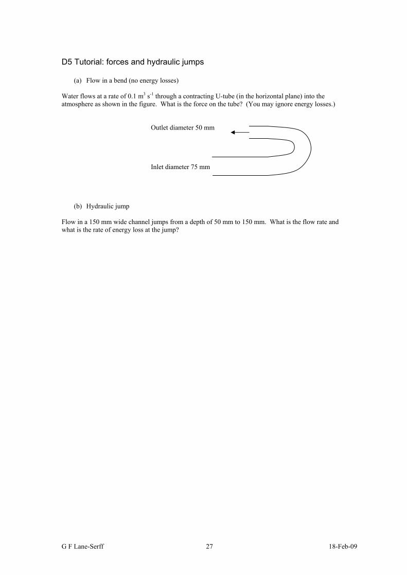
D5 Tutorial: forces and hydraulic jumps

(a) Flow in a bend (no energy losses) Water flows at a rate of 0.1 m3 s-1 through a contracting U-tube (in the horizontal plane) into the atmosphere as shown in the figure. What is the force on the tube? (You may ignore energy losses.)

Outlet diameter 50 mm

Inlet diameter 75 mm

(b) Hydraulic jump Flow in a 150 mm wide channel jumps from a depth of 50 mm to 150 mm. What is the flow rate and what is the rate of energy loss at the jump?


E Pipeflow

E1 Reynolds Experiment: Laminar and turbulent flow Osborne Reynolds (1842-1912), Professor at Manchester University Derived an expression for the relative size of viscous and other accelerations (Reynolds number: see below) and demonstrated the importance of this relation by examining the nature of flow in a pipe.

"direct" (laminar) motion

"sinuous" (turbulent) motion Reynolds Number (Re) Consider flow in a pipe of diameter D with typical speed U.

Volume of fluid element

V = (π/4)D2 dx. So mass of fluid element

m = ρ(π/4)D2 dx. Area of fluid element in contact with pipe wall

πD dx. Typical size of velocity gradient

∂u∂r ~

UD

So typical size of viscous force on fluid element (ignore π)

FV ~ µ UD D dx ~ µ U dx

Thus accelerations due to viscous forces (again ignoring constants)

aV = FV/m ~ µ U dxρD2 dx =

ν U D2 ,

where ν = µρ is the kinematic viscosity.

dye injected

dye injected

D U

dx


But we can find another scale for accelerations

a ~ u∂u∂x ~ U

UD =

U2

D .

The ratio of this to the viscous acceleration is given by

U2

D D2

ν U = U D

ν ≡ Re

The Reynolds number (usually denoted by Re) is the ratio of inertial to viscous accelerations and is equal to a velocity scale × length scale / kinematic viscosity. Note that the dimensions cancel out (ν has units m2 s-1), so that the Reynolds number is a dimensionless number and will be the same whatever units are used to measure lengths and times. High Re - Turbulent flow (Re > 4000 for typical pipe flows). Inertial forces dominate. Low Re - Laminar flow (Re < 2000 for typical pipe flows). Viscous forces dominate. At intermediate Re the flow is "transitional" and may have intermittent "bursts" of turbulence in an otherwise smooth flow. For flow in a pipe, the nature of the flow doesn't depend on the individual parameters (U, D, ν) but on the combination Re (the velocity scale used is usually the average velocity U=Q/A). Examples Flow rate Q = 0.01 m3 s-1 of water (ν = 10-6 m2 s-1), in a pipe of diameter D = 100 mm. What is the Reynolds number and the expected type of flow?

A = (π/4) 0.12 = 7.85×10-3 m2. U = Q/A = 1.27 m s-1. Re = UD/ ν = 1.27×0.1/10-6 = 127 000, so the flow will be turbulent. Flow rate Q = 10-6 m3 s-1 (= 1 cm3 s-1) of olive oil (ν = 10-4 m2 s-1), in a pipe of diameter D = 5 mm. What is the Reynolds number and the expected type of flow?

A = (π/4) 0.0052 = 1.96×10-5 m2. U = Q/A = 0.051 m s-1. Re = UD/ ν = 0.051×0.005/10-4 = 2.6, so the flow will be laminar. Most fluid flows in civil engineering are at high Reynolds number (an exception is flows through porous media, e.g. groundwater, water filtration).

Flow U (m s-1) L (m) ν (m2 s-1) Re Water in a domestic pipe 2 0.01 10-6 2×104 Air flow past a building 5 10 1.5×10-5 3.3×106 River flow 2 5 10-6 107 Air flow through a doorway 0.5 2 1.5×10-5 6.7×104 Water percolating through sand 6×10-5 10-4 10-6 6×10-3


E2 Pipeflow: laminar flow Low Re, viscous forces are important. Laminar flow in a pipe (Poiseuille Flow) Smooth, steady flow. Expect velocity u to be a function of radius r, with u = 0 at r = R (no flow at the pipe wall) but do not expect the speed to vary along the pipe (at a given radius). Consider the forces on a cylindrical fluid element within the pipe:

Area of flat faces

A = πr2 Area of curved surface

S = 2πr dx Volume

V = πr2 dx Pressure forces Total pressure force = -dp A = -dp πr2. Viscous forces

The viscous force depends on the shear at that radius. Force per unit area (viscous stress)

= µ ∂u∂r

So total force = µ ∂u∂r S = µ

∂u∂r × 2πr dx

Here velocity decreases as r increases, so this is negative - the viscous forces tend to slow the fluid down. For steady flow which isn't changing along the pipe (du/dx = 0), the sum of the viscous and pressure forces must be zero.

-dp πr2 + µ ∂u∂r × 2πr dx = 0

centre-line u(r)

r dx

pA (p+dp)A


Rearranging gives,

2µ ∂u∂r = r

dpdx

If the pressure gradient driving the flow along the pipe is constant G = dpdx , then,

∂u∂r =

Gr2µ .

If the flow is being driven in the x-direction we expect the pressure to decrease as x increases, so G would be negative.

Integrating this up we get u = Gr2

4µ + constant. We find the constant by using u(R) = 0:

u = -G4µ (R2 - r2)

The velocity profile for laminar flow is parabolic. This flow is known as Poiseuille flow. The total flow rate is given by,

Q = ⌡⌠0

Ru 2πr dr = -

πGR4

8µ .

The average flow speed U = Q/A is

U = -GR2

8µ . = 12 Umax.

For viscous flows, velocity and flow rates are proportional to the pressure gradient. Note that energy is lost and Bernoulli's Equation no longer applies (or has to be adjusted to include energy losses). Example: viscous flow down inclined tube Here there is no significant pressure gradient driving the flow, but the component of gravity along the tube has the same effect:

ρg sin θ = -G For d = 3 mm, θ = 10°, with water we get,

U = -GR2

8µ = ρg sin θ d2

32µ = g sin θ d2

32ν = 9.81× sin10° 0.0032

32x10-6 = 0.47 m s-1.

Check Reynolds number:

Re = UD/ν = 1410 (just about laminar).

θ


E3 Flow from static reservoir (no energy losses) Now consider the case where we can ignore viscosity and energy losses. If the water is discharged into the atmosphere, then the pressure there is atmospheric (approximately the same as at the surface of the reservoir). Bernoulli's Equation reduces to,

h = u2

2g , so u = 2gh . (This is the speed a body falling from height h would have.)

The total head is given by the height of the water surface in the static reservoir, i.e. H = h.

H = u2

2g + p

ρg + z,

where p is the gauge pressure (relative to atmospheric). Thus in the pipe, the pressure is simply given by

p = - ρgz. Example Pipe diameter 200 mm.

u

h

z=0

3 m

2 m

4 m

A


Height of surface above outlet H = 3 + 4 = 7 m.

Speed of flow u = 2×g×7 = 11.7 m s-1. Area A = (π/4)d2 = 0.314 m2.

Thus flow rate Q = 11.7×0.314 = 3.67 m3 s-1 ( = 3670 litres/s).

Pressure at A (relative to atmospheric)

p = - ρgz = -1000×9.81×(4+3+2) = -88.3 kN m-2 = -88.3 kPa. (Note: for total heights over about 10 m, predicted pressures would be less than absolute zero, which is not possible.) Example An open rectangular tank 2m×3m×1m high is full of water. It is emptied through a tube of diameter 15mm, discharging to the atmosphere 2m below the bottom of the tank. How long does it take to empty? When the depth of water in the tank is h, the speed of the water coming out of the tube is given by,

u = 2gh ,

(assuming the vertical speed of the water surface is negligible and ignoring any energy losses).

The flow rate is Q = ua = 2gh π4 d2, where d = 0.015 m and a is the tube area.

The rate at which the water level descends is Q/A where A is the area of the tank (A = 6 m2).

2015.046

2

π

−=−=gh

AQ

dtdh

or dhdt = - 1.305×10-4 h .

So

∫∫=

=

−=

=

− ×−=ett

t

h

h

dtdhh0

42

3

2/1 101.305 .

Thus 2×(31/2 - 21/2) = 1.305×10-4 te or te = 4870 s (approximately one hour twenty minutes).

h 1 m

2 m


E4 Turbulent flow and head loss Head loss in pipes: Darcy's formula In Civil Engineering applications, flows are usually at high Reynolds numbers. Conservation of energy (Bernoulli's Equation) gave

H = u2

2g + p

ρg + z,

with H a constant. For flow in a pipe of constant diameter u is constant and so the dynamic head is constant. If Bernoulli's Equation applied we would expect the piezometric head to also remain constant. However, experiments show that the piezometric head falls, with the fall proportional to the length of the tube and the square of the speed (at high Reynolds number). This can be thought of as a drop in the total head. For a pipe of length l and diameter d, the drop is found to be,

hf =

λl

d

u2

2g ,

where λ is a constant, known as the friction factor. This expression is know as Darcy's formula. (It is convenient to keep it as a multiple of the dynamic head.) The constant λ depends on the relative roughness of the pipe (kS/d, where kS, or just k, is the size of the roughness - "bumps") and on the Reynolds number of the flow. For very large values of Re, λ becomes independent of Re and is approximately given by,

λ = (2 log10(3.7 d/kS))-2 Darcy's formula is sometimes expressed as

hf =

4fl

d

u2

2g ,

where f=λ/4. WARNING: Sometimes (especially in the USA) the symbol f is used for λ, giving a different f from that we've defined (by a factor of 4). When using published graphs and tables it is important to check which version of f or λ is used. Example For galvanized steel, the roughness scale kS = 0.15 mm. For a pipe of diameter 100 mm, d/kS = 667. Thus the friction factor (for high Re) is λ = 0.0217.

Typical roughness scales kS (mm) Riveted steel 1 - 10 Concrete 0.3 - 3 Wood stave 0.2 - 1 Cast iron 0.25 Galvanized steel 0.15 Steel or wrought iron 0.045 Drawn tubing 0.0015 Roughness tends to increase with age because of deposits and corrosion. Friction factor for laminar flow If there is a head loss of hf, then the corresponding pressure change is simply

∆p = hf ρg.

This gives a pressure gradient (along a pipe of length l) of

G = - ∆pl = -

hf ρgl .


For low Re, laminar flow, we found the average velocity was given by

U = -Gd2

32µ = hf ρg d2

32 µ l .

Rearranging gives

hf = 32µlUρgd2 =

l

d

64ν

Ud

U2

2g =

l

d

64

Re

U2

2g

Which is equivalent to Darcy's formula with λ =64/Re. Moody's Diagram At low Re (laminar flow) the pressure drop (and head loss) along a pipe is proportional to the velocity, while at very large Re the pressure drop is proportional to the square of the velocity. For a given relative roughness (kS/d), a plot of friction factor λ as a function of Reynolds number will have λ=64/Re at low Re, tending towards a constant λ=(2 log10(3.7 d/kS))-2 at high Re. At intermediate values of Re there is a transition between the laminar and very turbulent flows. For very smooth pipes, where the boundary layer is larger than the roughness elements, λ=0.316Re-1/4 gives good agreement with experiment up to Re = 105. A Moody Diagram shows the relationship between λ and Re for various relative roughnesses (kS/d). The plot is usually on logarithmic axes, so that the laminar formula λ=64/Re is a straight line. (WARNING: If you see a plot where the laminar formula is friction factor =16/Re, then this is a plot of f =λ/4, as described earlier. Older exam papers also give f instead of λ, and you will need to use λ=4f to get the correct results.) For the present course, we will assume that the flow can be described by a constant λ (rough pipe flow), or by laminar flow. At intermediate values calculations become more complicated because the flow depends on λ, but λ depends on Re which in turn depends on the flow. Thus an iterative procedure is usually needed to calculate the flow. Formulae that match the smooth pipe flow equation to the high Re (constant λ) values and the methods of using them will be dealt with in later courses. Example A flow Q = 0.1 m3 s-1 is flowing through a galvanized steel pipe of diameter 100 mm. What is the head loss over a distance of 15 m?

A = (π/4) 0.12 = 7.85×10-3 m2, kS = 0.15 mm, λ = 0.0217. u = Q/A = 12.7 m s-1

hf =

λl

d

u2

2g =

0.0217×15

0.1

12.72

2×9.81 = 26.8 m

Power loss = Q ρg hf = 26.3 kW.

Total head = dynamic head + piezometric head

piezometric head

dynamic head


E5 Pipeflow: other head losses Head loss coefficient We've already seen that the head loss along a pipe of length l is given by

hf =

λl

d

u2

2g .

There are other head losses (energy losses) caused by enlargements, contractions, bends, valves and other fittings. These are generally expressed in the form

hl = k

u2

2g .

In principle, the head loss coefficient, k, varies with Re but at large Re the head loss coefficient is effectively constant. (Warning: don't confuse the non-dimensional head loss coefficient k with the roughness length also unfortunately often denoted by k or kS.) Abrupt enlargement

hl =

1 -

A1A2

2 u1

2

2g =

A2

A1 - 1

2 u2

2

2g

(Proof later in F1.) As A2 → ∞, the "exit loss" (e.g. from a pipe into a reservoir) hl → u1

2

2g.

Abrupt contraction

hl = k u2

2

2g. As A1 → ∞, the "entry loss" (e.g. from a reservoir into a pipe) hl → 0.5 u2

2

2g

d2/d1 (diameter ratio) 0 0.2 0.4 0.6 0.8 k 0.5 0.45 0.38 0.28 0.14

Other entry losses

A1

u1

u2

A2

A1

u1 A2

u2

k = 1.0k = 0.5 k ≈ 0


Pipe fittings, typical losses Fitting 90° bend 90° corner 45° bend T (in-line) T (side) k 0.9 1.1 0.4 0.4 1.2 Example

A reservoir is drained through a 150 mm diameter pipe, 500 m long, with an exit to the atmosphere 10 m below the water surface in the reservoir. What is the discharge? (The friction factor for the pipe is λ =0.020.)

Energy at A = Energy at B + Energy losses from A to B

HA = HB + Hlosses

Hlosses = entry loss + pipe loss (assume no significant loss on exit to atmosphere)

10 = u2

2g + kentry u2

2g +

λl

d u2

2g

10 = u2

2g + 0.5 u2

2g +

0.020×500

0.15 u2

2g

10 = (1 + 0.5 + 66.7) u2

2g

u2

2g = 10/68.2 = 0.147, so u = 1.70 m s-1.

This gives Q = 0.030 m3 s-1.

(Check Re = ud/ν = 2.6×105.)

Note that most of the losses come from flow along the pipe. In practice ignoring entry and exit losses, and losses at bends and fittings does not usually lead to significant errors in most civil engineering applications. Junctions

HA = HJ + Hlosses(A toJ)

Also QA = QB + QC

HJ = HB + Hlosses(J to B)

HJ = HC + Hlosses(J to C)

10 m

A

B

A

J

C

B


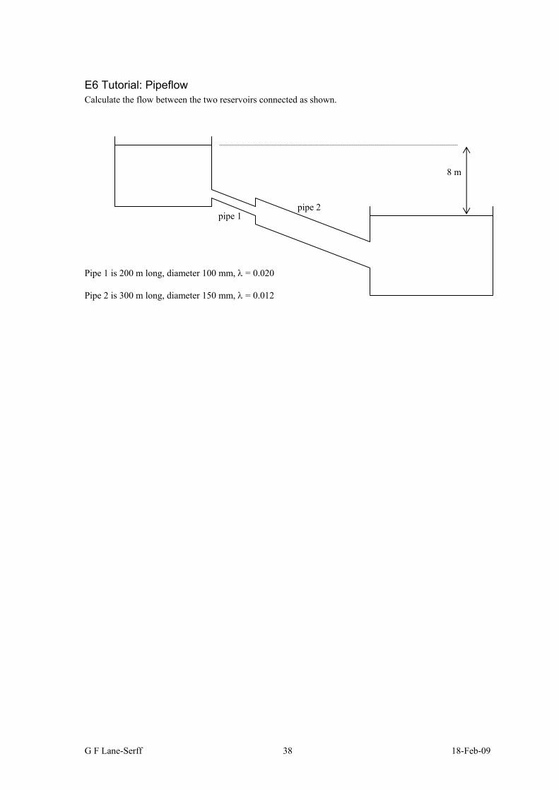
E6 Tutorial: Pipeflow Calculate the flow between the two reservoirs connected as shown. Pipe 1 is 200 m long, diameter 100 mm, λ = 0.020 Pipe 2 is 300 m long, diameter 150 mm, λ = 0.012

8 m

pipe 1 pipe 2


F Energy and momentum: further applications

F1 Sharp expansions and orifice meters Sharp expansion

The pressure on the face of the vertical surface just downstream of the expansion is found to be close to p1. (Weak radial accelerations there.)

If we assumed there was no energy loss we would find,

(p1 - p2) = ρ (u22 - u1

2)/2,

= ρ u (u2 - u1), where u = (u2 + u1)/2 is the average of u2 and u1. However, applying the momentum principle to a control volume as marked on the diagram (and using the observation that the pressure just downstream of the expansion is close to p1 over the face of the vertical surface), we find

(p1 - p2) A2 = ρQ (u2 - u1) so,

(p1 - p2) = ρ u2 (u2 - u1). If the head loss is hl,

H1 = H2 + hl

lhg

pg

ug

pg

u+

ρ+=

ρ+ 2

221

21

22

gpp

guuhl ρ

−+

−= 21

22

21

2

( )

guuu

guuhl ρ

−ρ+

−= 122

22

21

2

guuuuuhl 2

22 1222

22

21 −+−

=

hl = ( )u1 - u2

2

2g

But

Q = u1 A1 = u2 A2, ⇒ u2 = u1 (A1/A2).

u1 u2


so,

hl = ( )u1 - u1(A1/A2) 2

2g ,

or

hl =

1 -

A1A2

2 u1

2

2g =

A2

A1 - 1

2 u2

2

2g

(as given in E5). Orifice meter Similar to a venturimeter (see D2) but much more energy is lost with this type of flow. We have a sharp contraction followed by a sharp expansion. We can use a similar formula as for the venturimeter,

−

∆=

1

2

22

21

1

AA

hgCAQ d ,

but now Cd ≈ 0.6. While it is possible to estimate Cd theoretically, in practice for accurate measurements the orifice meter will be calibrated to find Cd.

A1 A2

p1 p2


F2 Momentum principle: effects of gravity Flow around a pipe bend (continuation of D3) b) change in area (A1 ≠ A2) and now include gravity Conservation of mass

Q = uA = u1A1 = u2A2 If there are no (or negligible) energy losses

22

22

11

21

22z

gp

guHz

gp

gu

++==++ρρ

The gravitational force is ρVg (downwards). Example Water is flowing at 0.05 m3 s-1 through a 90° reducing elbow turning from horizontal to vertical, emerging into the atmosphere with the exit 0.25 m above the large pipe. If the diameter reduces from 100 mm to 50 mm, and the volume of the fitting is given as 1.6×10-3 m3, what force is required to keep the fitting in place? (For the force on the elbow, we need the difference in pressure from atmospheric, so take p2 = 0.)

V (Volume of section)

u1

u2

A1 A2

z1

z2

z = 0

u1

u2

0.25 m


Conservation of mass

Q = 0.05 m3 s-1, A1 = (π/4) 0.12 = 7.85×10-3 m2; A2 = (π/4) 0.052 = 1.96×10-3 m2;

and thus u1 = Q/A1 = 6.37 m s-1; u2 = Q/A2 = 25.5 m s-1;

giving velocities u1 = (6.37, 0.0) m s-1; u2 = (0.0, 25.5) m s-1. Assuming no energy loss in the bend,

22

22

11

21

22z

gp

guHz

gp

gu

++==++ρρ

,

25.0100081.9

081.92

5.250100081.981.92

37.6 21

2+

×+

×=+

×+

×p ,

so, p1 = 3.07×105 N m-2.

(In practice there are likely to be energy losses.)

Horizontal forces (acting on fluid) vertical forces (acting on fluid)

p1 A1 + Fx = 0 - ρQu1 -p2 A2 + Fz - ρVg = ρQu2 - 0. Where the force by the fitting on the fluid is F = (Fx,Fz). Thus F = (-2730, 1290) N, and the force by the fluid on the fitting is -F = (2730, -1290) N. Thus the force needed to keep the fitting in place is F.

u1

u2

F (force needed to keep fitting in place)

F (force by fitting on fluid)

-F (force by fluid on fitting)


F3 Tutorial: Gravity and flow measurement Flow in a bend with energy loss What would be the result to the previous example (flow in a bend with gravity) where the applied pressure p1 is the same but you assume a head loss in the bend given by

hl = k u1

2

2g, with k=0.9?

Orifice meter Air flowing through a tube of diameter 10cm, with a sharp orifice of diameter 5 cm. The pressure drop is measured with a water manometer giving a change in level of 10 cm. What is the flow rate? (Assume Cd = 0.6.)

hydraulics 1: course notes the pressure increases as z decreases (or depth increases). integrating...

Documents